Date:

Gravitational wave signals in an Unruh-DeWitt detector

Tomislav Prokopec^♢

Institute for Theoretical Physics, Spinoza Institute & EMME$\Phi$

Utrecht University, Princetonplein 5, 3584 CC Utrecht, The Netherlands

Abstract

We firstly generalize the massive scalar propagator for planar gravitational waves propagating on Minkowski space obtained recently in Ref. [1]. We then use this propagator to study the response of a freely falling Unruh-DeWitt detector to a gravitational wave background. We find that a freely falling detector completely cancels the effect of the deformation of the invariant distance induced by the gravitational waves, such that the only effect comes from an increased average size of scalar field vacuum fluctuations, the origin of which can be traced back to the change of the surface in which the gravitational waves fluctuate. The effect originates from the quantum interference between propagation on off-shell detector’s trajectories which probe different spatial gravitational potential induced by the gravitational backreaction from gravitational waves, and it is therefore purely quantum. When resummed over classical graviton insertions, gravitational waves generate cuts on the imaginary axis of the complex $\Delta\tau$-plane (where $\Delta\tau=\tau-\tau^{\prime}$ denotes the difference of proper times), and the discontinuity across these cuts is responsible for a continuum of energy transitions induced in the Unruh-DeWitt detector. Not surprisingly, we find that the detector’s transition rate is exponentially suppressed with increasing energy and the mass of the scalar field. What is surprising, however, is that the transition rate is a non-analytic function of the gravitational field strain. This means that, no matter how small is the gravitational field amplitude, expanding in powers of the gravitational field strain cannot approximate well the detector’s transition rate. We present numerical and approximate analytical results for the detector’s transition rate both for circularly polarized and for polarized monochromatic, unidirectional, gravitational waves.

^♢ e-mail: T.Prokopec@uu.nl

1 Introduction

In this work we calculate the response of a freely falling Unruh-DeWitt detector which couples to a massless or massive scalar field fluctuating in the presence of planar gravitational waves propagating on Minkowski spacetime. This work builds on earlier studies [2, 3, 4, 7, 8, 9, 1], which address some aspects of the problem of how planar gravitational waves affect scalar fields. In particular the authors of Ref. [9] investigate the response of freely-falling and accelerating Unruh-DeWitt detectors [10, 11, 12] in the presence of gravitational waves. In this work we generalize their analysis by using the propagator recently obtained in Ref. [1]. For simplicity, we do not analyze here the response of the detector moving along noninertial trajectories.

The model. In this work we consider a real, self-interacting scalar field $\phi(x)$ whose action and Lagrangian are,

$$S[\phi]=\int d^{D}x\sqrt{-g}\,{\cal L}_{\phi}\,,\qquad{\cal L}_{\phi}=-\frac{1}{2}(\partial_{\mu}\phi)(\partial_{\nu}\phi)g^{\mu\nu}-\frac{m^{2}}{2}\phi^{2}-\frac{\lambda}{4!}\phi^{4}\,,\quad$$ (1.1)

where $g={\rm det}[g_{\mu\nu}]$, $g^{\mu\nu}$ is the inverse of the metric tensor $g_{\mu\nu}$, $m$ is the field’s mass and $\lambda$ is the self-interaction coupling strength. We work in natural units in which $c=1$, but keep the dependence on $\hbar$ explicit. This means that the dimension of the field $\phi$ and the mass $m$ is ${\rm m}^{-1}$, and $\lambda$ is dimensionless. To restore the physical dimension of $m$, one ought to rescale it as, $m\rightarrow mc/\hbar$.

1.1 Gravitational waves

We are interested in understanding the effects of gravitational waves on scalar fields. A convenient representation for a gravitational wave background is,

$$g_{\mu\nu}(x)=\eta_{\mu\nu}+h_{\mu\nu}(x)\,,$$ (1.2)

where $h_{\mu\nu}(x)$ is a perturbation of the metric tensor $g_{\mu\nu}$ around flat Minkowski space, characterized by Minkowski metric $\eta_{\mu\nu}$, which is in Cartesian coordinates a $D\times D$ diagonal matrix of the form, $\eta_{\mu\nu}={\rm diag}(-1,1,1,\dots)$. In the traceless-transverse gauge (in which the gravitational field perturbation $h_{\mu\nu}$ is gauge invariant to linear order in the gravitational field), planar gravitational waves moving in the $x^{D-1}$ direction ($x^{D-1}\rightarrow z$ when $D=4$) satisfy $h_{0\mu}=0$ and

$$h_{ij}(u)=\left(\begin{array}[]{ccccc}h_{xx}(u)&h_{xy}(u)&\cdots&h_{xD-2}(u)&0\cr h_{xy}(u)&h_{yy}(u)&\cdots&h_{yD-2}(u)&0\cr\vdots&\vdots&\vdots&\cdots&\vdots\cr h_{xD-2}(u)&h_{yD-2}(u)&\cdots&h_{D-2D-2}(u)&0\cr 0&0&\cdots&0&0\cr\end{array}\right)\,,$$ (1.3)

where $u=t-x^{D-1}$ is a lightcone coordinate. Note that some of the elements of $h_{ij}$ in Eq. (1.3) may vanish. In $D=4$ dimensions this simplifies to planar gravitational waves with nonvanishing elements in the $xy-$plane. In practical calculations it is often convenient to simplify (1.3) by assuming that nonvanishing elements of $h_{ij}$ are in the upper left $2\times 2$ block.

In this work we generalize the monochromatic wave background considered in Ref. [1] to the case when the gravitational wave strain, $h_{ij}=h_{ij}(u)$, is characterized by a general function of $u$ propagating in the $x^{D-1}$ direction. Motivated by the form of gravitational waves emitted by realistic sources, whose wave form can be decomposed into the fundamental mode of frequency $\omega_{g}$, and the higher overtones (whose frequencies are $n\omega_{g}$), we shall consider gravitational waves of the form,

$$h_{ij}(u)=\sum_{n=1}^{\infty}h_{ij}^{(n)}\cos(n\omega_{g}u+\psi_{ij}^{(n)})\,,$$ (1.4)

where $h_{ij}^{(n)}$ and $\psi_{ij}^{(n)}$ are the (time independent) gravitational field amplitudes and phases of the $n$-th harmonic. Such elliptically polarized gravitational waves are formed by binary systems whose components harbor angular momentum and/or strong magnetic fields [13, 14]. It is important to keep in mind that, even when gravitational waves are emitted as circularly polarized, the perceived amplitudes of the $+$ and $\times$ polarizations will differ, unless the source is face on, i.e. the inclination angle is zero. This means that the only fixed characteristic of observed gravitational waves is the relative phase difference, $\Delta\psi=\psi_{+}-\psi_{\times}=\pm\pi/2$.

The gravitational waves considered here have a phase velocity, $\vec{v}_{\rm ph}=\hat{z}$, and are often referred to as the positive frequency solutions. In addition there are negative frequency gravitational waves, with an opposite phase velocity ($\vec{v}_{\rm ph}=-\hat{z}$), for which $h_{ij}=h_{ij}(v)$, with $v=t+z$ ($v=t+x^{D-1}$ in the $D$ dimensional case). Sufficiently close to the gravitational wave source the gravitational wave propagates radially, such that in a relatively small spatial volume one can approximate the wave by $h_{ij}(u)$.

2 Scalar propagator

Variation of the action (1.1) gives a Klein-Gordon equation satisfied by the scalar field operator $\hat{\phi}(x)$,

$$\big{(}\Box-m^{2}\big{)}\hat{\phi}(x)=0\,,$$ (2.1)

where $\Box=\frac{1}{\sqrt{-g}}\partial_{\mu}\sqrt{-g}g^{\mu\nu}\partial_{\nu}$ is the d’Alembertian operator as it acts on a scalar field, and we have neglected in Eq. (2.1) the quartic self-coupling. The positive and negative frequency Wightman functions are defined as the following two-point functions,

$$i\Delta^{(+)}(x;x^{\prime})\!\! = \!\!\left\langle\Omega\right|\hat{\phi}(x)\hat{\phi}(x^{\prime})\left|\Omega\right\rangle\,,$$ (2.2)

$$i\Delta^{(-)}(x;x^{\prime})\!\! = \!\!\left\langle\Omega\right|\hat{\phi}(x^{\prime})\hat{\phi}(x)\left|\Omega\right\rangle\,,$$ (2.3)

where $\left|\Omega\right\rangle$ denotes a state of the scalar field, which for simplicity we choose to be the vacuum state. When the field operator in Eq. (2.1) is expanded in terms of the momentum space mode functions, one can reduce the problem of obtaining the Wightman functions to performing the momentum integrals in Eqs. (5.2–5.3) over products of the mode functions. These integrals can be performed by a straightforward generalization of the method used in Ref. [1], whose the main steps outline in Appendix A. From Eqs. (5.14–5.17) it immediately follows,

$$i\Delta^{(\pm)}(x;x^{\prime})=\frac{\hbar m^{D-2}}{(2\pi)^{\frac{D}{2}}[\gamma(u)\gamma(u^{\prime})]^{\frac{1}{4}}\sqrt{{\rm det}[{\cal G}^{ij}](u;u^{\prime})}}\frac{K_{\frac{D-2}{2}}\big{(}m\sqrt{\Delta{\bar{x}}_{(\pm)}^{2}}\,\big{)}}{\big{(}m\sqrt{\Delta{\bar{x}}_{(\pm)}^{2}}\,\big{)}^{\frac{D-2}{2}}}\,,$$ (2.4)

where $K_{\nu}(z)$ denotes the modified Bessel function of the second kind, and $\Delta{\bar{x}}_{(\pm)}^{2}(x;x^{\prime})$ are the deformed distance functions, which in lightcone coordinates can be written as,

$$\Delta{\bar{x}}_{(\pm)}^{2}(x;x^{\prime})\!\! = \!\!-(\Delta u\!\mp\!i\epsilon)(\Delta v\!\mp\!i\epsilon)+\left(\!\begin{array}[]{cccc}\Delta x&\Delta y&\cdots&\Delta x^{D-2}\end{array}\!\right)\!\cdot\!\mathbf{\cal G}(u;u^{\prime})\!\cdot\!\left(\!\begin{array}[]{c}\Delta x\cr\Delta y\cr\vdots\cr\Delta x^{D-2}\cr\end{array}\!\right)\,,\qquad$$ (2.10)

and in Cartesian coordinates,

$$\Delta{\bar{x}}_{(\pm)}^{2}(x;x^{\prime})\!\! = \!\!-(\Delta t\mp i\epsilon)^{2}+\left(\!\begin{array}[]{cccc}\Delta x&\Delta y&\cdots&\Delta x^{D-2}\end{array}\!\right)\!\cdot\!\mathbf{\cal G}(u;u^{\prime})\!\cdot\!\left(\!\begin{array}[]{c}\Delta x\cr\Delta y\cr\vdots\cr\Delta x^{D-2}\cr\end{array}\!\right)+\Delta x_{D-1}^{2}\,,\qquad$$ (2.16)

where $\Delta x^{\mu}=x^{\mu}-{x^{\prime}}^{\mu}$, where the deformation matrix ${\cal G}_{ij}(u;u^{\prime})$ is given by,

$${\cal G}_{ij}(u;u^{\prime})\!\! = \!\!\left(\!\!\begin{array}[]{cccc}{\cal G}_{xx}(u;u^{\prime})&{\cal G}_{xy}(u;u^{\prime})&\cdots&{\cal G}_{xD-2}(u;u^{\prime})\cr{\cal G}_{xy}(u;u^{\prime})&{\cal G}_{yy}(u;u^{\prime})&\cdots&{\cal G}_{yD-2}(u;u^{\prime})\cr\vdots&\vdots&\vdots&\vdots\cr{\cal G}_{xD-2}(u;u^{\prime})&{\cal G}_{yD-2}(u;u^{\prime})&\cdots&{\cal G}_{yD-2}(u;u^{\prime})\cr\end{array}\!\!\right)\,.\qquad$$ (2.21)

Note that ${\cal G}_{ij}(u;u^{\prime})$ is the inverse of the corresponding momentum space deformation matrix ${\cal G}^{ij}(u;u^{\prime})$, ${\cal G}^{ik}(u;u^{\prime}){\cal G}_{kj}(u;u^{\prime})=\delta^{i}_{\;j}$. The general form of ${\cal G}^{ij}(u;u^{\prime})$ is,

$${\cal G}^{ij}(u;u^{\prime})(u;u^{\prime})\!\! = \!\!\frac{1}{\Delta u}\int_{u^{\prime}}^{u}\left(\!\!\begin{array}[]{cccc}g^{xx}(\bar{u})&g^{xy}(\bar{u})&\cdots&g^{xD-2}(\bar{u})\cr g^{xy}(\bar{u})&g^{yy}(\bar{u})&\cdots&g^{yD-2}(\bar{u})\cr\vdots&\vdots&\vdots&\vdots\cr g^{xD-2}(\bar{u})&g^{yD-2}(\bar{u})&\cdots&g^{D-2D-2}(\bar{u})\cr\end{array}\!\!\right){\rm d}\bar{u}\,,\qquad$$ (2.26)

where $g^{ij}(u)$ denote the inverse of $g_{ij}(u)$. For example, for gravitational waves oscillating in the $xy$ plane, only the distances in this plane (which we denote by $\perp$) get deformed, such that the nontrivial elements of the deformation matrix are,

$${\cal G}^{ij}_{\perp}(u;u^{\prime})\!\! = \!\!\frac{1}{\Delta u}\int_{u^{\prime}}^{u}\left(\!\!\begin{array}[]{cc}g^{xx}(\bar{u})&g^{xy}(\bar{u})\cr g^{xy}(\bar{u})&g^{yy}(\bar{u})\cr\end{array}\!\!\right){\rm d}\bar{u}$$ (2.29)

$$= \!\!\frac{1}{\Delta u}\int_{u^{\prime}}^{u}\frac{1}{\gamma(u)}\left(\!\!\begin{array}[]{cc}g_{yy}(\bar{u})&-g_{xy}(\bar{u})\cr-g_{xy}(\bar{u})&g_{xx}(\bar{u})\cr\end{array}\!\!\right){\rm d}\bar{u}\,,\qquad$$ (2.32)

where $\gamma(u)={\rm det}[g_{ij}(u)]$. For monochromatic, circularly polarized gravitational waves in linear representation one obtains (see section 3 of Ref. [1]),

$${\cal G}_{ij}^{\perp}(u;u^{\prime})\!\! = \!\!\frac{1}{\gamma{\rm det}[{\cal G}_{\perp}^{ij}](u;u^{\prime})}\left(\!\!\begin{array}[]{cc}1\!+\!h\frac{\sin(\omega_{g}u)-\sin(\omega_{g}u^{\prime})}{\omega_{g}\Delta u}&-h\frac{\cos(\omega_{g}u)-\cos(\omega_{g}u^{\prime})}{\omega_{g}\Delta u}\cr-h\frac{\cos(\omega_{g}u)-\cos(\omega_{g}u^{\prime})}{\omega_{g}\Delta u}&1\!-\!h\frac{\sin(\omega_{g}u)-\sin(\omega_{g}u^{\prime})}{\omega_{g}\Delta u}\cr\end{array}\!\!\right)\,,$$ (2.35)

$${\rm det}\left[{\cal G}_{\perp}^{ij}(u;u^{\prime})\right]\!\! = \!\!\frac{1}{\gamma^{2}}\bigg{[}1\!-\!h^{2}j^{2}_{0}\Big{(}\frac{\omega_{g}\Delta u}{2}\Big{)}\bigg{]}\,,\quad$$ (2.36)

where $j_{0}(z)=\sin(z)/z$ is the spherical Bessel function, $\gamma(u)={\rm det}[g_{ij}(u)]=1-h^{2}$ is time independent, $h=h_{+}=h_{\times}$, and $h_{+}=h_{xx}=-h_{yy}$ and $h_{\times}=h_{xy}$ are the amplitudes of the two polarizations. The matrix $\mathbf{\cal G}_{ij}^{\perp}(u;u^{\prime})$ deforms distances in position space according to Eqs. (2.10–2.16).

On the other hand, for singly polarized monochromatic waves fluctuating in the $xy$-plane one obtains for the $(+)$-polarized waves ($h_{+}\neq 0$, $h_{\times}=0$),

$${\cal G}^{ij}_{\perp}=\frac{2}{\omega_{g}\Delta u}\frac{1}{\sqrt{1\!-\!h_{+}^{2}}}\left\{\left(\!\!\begin{array}[]{cc}\text{arctan}\bigg{[}\sqrt{\frac{1-h_{+}}{1+h_{+}}}\tan\Big{(}\frac{\omega_{g}u}{2}\Big{)}\bigg{]}&0\cr 0&\text{arctan}\bigg{[}\sqrt{\frac{1+h_{+}}{1-h_{+}}}\tan\Big{(}\frac{\omega_{g}u}{2}\Big{)}\bigg{]}\cr\end{array}\!\!\right)\!-\!(u\rightarrow u^{\prime})\right\},$$ (2.37)

and for the $(\times)$-polarized waves ($h_{+}=0$, $h_{\times}\neq 0$),

$${\cal G}^{ij}_{\perp}=\frac{1}{\omega_{g}\Delta u}\frac{1}{\sqrt{1\!-\!h_{\times}^{2}}}\left\{\left(\!\!\begin{array}[]{cc}\text{arctan}\bigg{[}\frac{1}{\sqrt{1\!-\!h_{\times}^{2}}}\tan(\omega_{g}u)\bigg{]}&-\text{arctan}\bigg{[}\frac{h_{\times}}{\sqrt{1-h_{\times}^{2}}}\sin(\omega_{g}u)\bigg{]}\cr-\text{arctan}\bigg{[}\frac{h_{\times}}{\sqrt{1-h_{\times}^{2}}}\sin(\omega_{g}u)\bigg{]}&\text{arctan}\bigg{[}\frac{1}{\sqrt{1-h_{\times}^{2}}}\tan(\omega_{g}u)\bigg{]}\cr\end{array}\!\!\right)\!-\!(u\rightarrow u^{\prime})\right\},$$ (2.38)

respectively.

From the Wightman functions (2.4) one can easily construct the Feynman propagator. In lightcone coordinates we have,

$$i\Delta_{F,LC}(x;x^{\prime})\!\!\! \equiv \!\!\!\Theta(\Delta u)i\Delta^{(+)}(x;x^{\prime})\!+\!\Theta(-\Delta u)i\Delta^{(-)}(x;x^{\prime})$$ (2.39)

$$= \!\!\frac{\hbar m^{D-2}}{(2\pi)^{\frac{D}{2}}[\gamma(u)\gamma(u^{\prime})]^{\frac{1}{4}}\sqrt{{\rm det}[{\cal G}^{ij}](u;u^{\prime})}}\frac{K_{\frac{D-2}{2}}\big{(}m\sqrt{\Delta{\bar{x}}_{F,LC}^{2}}\,\big{)}}{\big{(}m\sqrt{\Delta{\bar{x}}_{F,LC}^{2}}\big{)}^{\frac{D-2}{2}}},\qquad\;\;$$

and in Cartesian coordinates,

$$i\Delta_{F}(x;x^{\prime})\!\! \equiv \!\!\Theta(\Delta t)i\Delta^{(+)}(x;x^{\prime})+\Theta(-\Delta t)i\Delta^{(-)}(x;x^{\prime})$$ (2.40)

$$= \!\!\frac{\hbar m^{D-2}}{(2\pi)^{\frac{D}{2}}[\gamma(u)\gamma(u^{\prime})]^{\frac{1}{4}}\sqrt{{\rm det}[{\cal G}^{ij}](u;u^{\prime})}}\frac{K_{\frac{D-2}{2}}\big{(}m\sqrt{\Delta{\bar{x}}_{F}^{2}}\,\big{)}}{\big{(}m\sqrt{\Delta{\bar{x}}_{F}^{2}}\big{)}^{\frac{D-2}{2}}}\,.\qquad$$

Both propagators (2.39–2.40) are suitable for perturbative studies, the former for the initial value problem defined on an $u={\rm constant}$ hypersurface, the latter on a $t={\rm constant}$ hypersurface. However, the two $i\epsilon$ prescriptions differ,

$$\Delta{\bar{x}}_{F,LC}^{2}(x;x^{\prime})\!\! = \!\!-(|\Delta u|-i\epsilon)(\pm\Delta v-i\epsilon)\!+\!\|\Delta\vec{\bar{x}}_{\perp}\|^{2}\,,$$

$$\Delta{\bar{x}}_{F}^{2}(x;x^{\prime})\!\! = \!\!-(|\Delta t|-i\epsilon)^{2}\!+\!\|\Delta\vec{\bar{x}}\|^{2}\,.\qquad\quad$$ (2.41)

That means that the imaginary parts of the propagators differ. Both prescriptions are legitimate, as they are designated to study inequivalent perturbative evolution problems.

From Eqs. (2.39–2.40) one easily obtains the corresponding Dyson propagators,

$$i\Delta_{D,LC}(x;x^{\prime})=\big{[}i\Delta_{F,LC}(x;x^{\prime})\big{]}^{*}\,,\qquad i\Delta_{D}(x;x^{\prime})=\big{[}i\Delta_{F}(x;x^{\prime})\big{]}^{*}\,,\qquad$$ (2.42)

which are important for studying time evolution of Hermitian operators in interacting quantum field theories.

One-loop results. In what follows we briefly summarize the one-loop calculations from Ref. [1] for the generalized gravitational waves of the form (1.3).

For the one-loop effective action calculation and one-loop scalar mass induced by the scalar self-interaction, one needs the coincident propagator (2.39–2.40), which is of the same form as in Eq. (4.4) of Ref. [1],

$$i\Delta_{F}(x;x)=\frac{\hbar m^{D-2}}{(4\pi)^{D/2}\sqrt{\gamma(u){\rm det}[{\cal G}^{ij}(u;u)]}}\Gamma\Big{(}1-\frac{D}{2}\Big{)}\,,$$ (2.43)

where $\gamma(u)={\rm det}[g_{ij}]$ and ${\rm det}[{\cal G}^{ij}(u;u)]$ is the determinant of the ${\cal G}^{ij}(u;u)$ matrix in Eq. (2.26) evaluated at spacetime coincidence. Applying the l’Hospital rule to Eq. (2.32) yields,

$${\cal G}^{ij}(u;u)\!\! = \!\!\left(\!\!\begin{array}[]{cccc}g^{xx}(u)&g^{xy}(u)&\cdots&g^{xD-2}(u)\cr g^{xy}(u)&g^{yy}(\bar{u})&\cdots&g^{yD-2}(u)\cr\vdots&\vdots&\vdots&\vdots\cr g^{xD-2}(u)&g^{xD-2}(u)&\cdots&g^{D-2D-2}(u)\cr\end{array}\!\!\right)\equiv g^{ij}(u)\,,\qquad$$ (2.48)

from which it immediately follows that, ${\rm det}[{\cal G}^{ij}](u;u)={\rm det}[g^{ij}(u)]=1/\gamma(u)$, and therefore,

$$\gamma(u){\rm det}[{\cal G}^{ij}(u;u)]=1\,.$$ (2.49)

This shows that both, the one-loop effective action and the one-loop scalar mass reduce to those of Minkowski space in Eqs. (4.12) and (4.15) of Ref. [1].

The calculation of the one-loop energy momentum tensor is more involved, but the procedure is the same as for the polarized gravitational waves in linear representation in section 5 of Ref. [1], and the resulting renormalized energy momentum tensor is identical in form as in Eqs. (5.29-5.30) of Ref. [1],

$$\langle\Omega|T^{*}[\hat{T}^{\rm ren}_{\mu\nu}(x)]|\Omega\rangle\!\! = \!\!-\frac{\hbar m^{4}}{64\pi^{2}}\left[\ln\left(\frac{m^{2}}{4\pi\mu^{2}}\right)\!+\!\gamma_{E}\!-\!\frac{3}{2}\right]g_{\mu\nu}(u)-\frac{\hbar m^{2}}{96\pi^{2}}\left[\log\left(\frac{m^{2}}{4\pi\mu^{2}}\right)\!+\!\gamma_{E}\!-\!1\right]G_{\mu\nu}(u)\,,\qquad\;\;$$ (2.50)

where $G_{\mu\nu}(u)$ is the classical Einstein tensor associated with the metric in Eqs. (1.2–1.3). The counterterms needed to renormalize (2.50) are generated by the cosmological constant action and the Hilbert-Einstein action, as detailed in Ref. [1]. Upon recalling that gravitational waves carry a classical (Lifshitz) energy-momentum tensor, $T_{\mu\nu}^{\rm class}=-G_{\mu\nu}(u)/(8\pi G)$, the result in Eq. (2.50) can be intuitively understood as the one-loop scalar matter energy momentum tensor induced by the leading quantum response of the massive scalar field to passing gravitational waves. The result (2.50) cannot be directly compared with that of Ref. [15], where the author considered the one-loop energy-momentum tensor of a massive scalar field observed in a distant future (in which the vacuum state reduces to that of Minkowski space) and argued that the one-loop energy momentum tensor is identical to that in Minkowski vacuum. Note also that, if the gravitational wave amplitude is adiabatically switched off, the result in Eq. (2.50) reduces to the trivial (Minkowski vacuum) result of Ref. [15].

3 Unruh-DeWitt detector

In this section we study the response of a freely falling Unruh-DeWitt detector [10, 11, 12] moving in the background of gravitational waves which propagate in the $z$-direction. This work generalizes the analysis of Ref. [9].

Freely falling observers. The line element for the problem at hand can be written from Eq. (1.2) as,

$${\rm d}s^{2}=-{\rm d}t^{2}+{\rm d}x^{i}g_{ij}(u){\rm d}x^{j}=-{\rm d}u{\rm d}v+{\rm d}x^{i}g^{\perp}_{ij}(u){\rm d}x^{j}\,,$$ (3.1)

where $g^{\perp}_{ij}(u)$ is a $(D-2)\times(D-2)$ dimensional symmetric metric tensor (in $D=4$ it reduces to a $2\times 2$ dimensional symmetric metric). Useful killing vectors are, ${K}_{v}=\partial_{v}$ and $K_{i}=\partial_{i}\;(i=1,2,\cdots,D-2)$, from which one obtains the corresponding conserved momenta, 

$$P_{v}=-(K_{v})_{\mu}\frac{{\rm d}x^{\mu}}{{\rm d}\tau}=\frac{1}{2}\frac{{\rm d}u}{{\rm d}\tau}\,,\qquad P_{i}=(K_{i})_{j}\frac{{\rm d}x^{j}}{{\rm d}\tau}=g^{\perp}_{ij}(u)\frac{{\rm d}x^{j}}{{\rm d}\tau}\,,\qquad(i,j=1,2,\cdots,D-2)\,,$$ (3.2)

where (for a later convenience) we chose the geodesic time $\lambda=\tau$ to be the proper time $\tau$, defined by ${\rm d}\tau^{2}=-{\rm d}s^{2}$. Upon inserting these equations into the line element (3.1) and dividing by $-{\rm d}\tau^{2}$ one obtains,

$$1=\frac{{\rm d}u}{{\rm d}\tau}\frac{{\rm d}v}{{\rm d}\tau}-\frac{{\rm d}x^{i}}{{\rm d}\tau}g^{\perp}_{ij}(u)\frac{{\rm d}x^{j}}{{\rm d}\tau}=2P_{v}\frac{{\rm d}v}{{\rm d}\tau}-P_{i}g_{\perp}^{ij}(u)P_{j}\,.$$ (3.3)

This generates the geodesic equation for ${\rm d}v/{\rm d}\tau$,

$$\frac{{\rm d}v}{{\rm d}\tau}=\frac{1}{2P_{v}}\left(1+P_{i}g_{\perp}^{ij}(u)P_{j}\right)\,,$$ (3.4)

whose formal solution is,

$$v(\tau)=v_{0}+\frac{1}{2P_{v}}\left(\tau+\frac{P_{i}}{2P_{v}}\int_{u_{0}}^{u}{\rm d}\bar{u}g_{\perp}^{ij}(\bar{u})P_{j}\right)\,,\qquad(v_{0}\equiv v(0),\;u_{0}\equiv u(0))\,,$$ (3.5)

where we made use of, ${\rm d}u/{\rm d}\tau=2P_{v}$. Next, one can solve equations (3.2) to obtain,

$$u(\tau)\!\! = \!\!u_{0}+2P_{v}\tau\,,\qquad(u_{0}\equiv u(0))$$ (3.6)

$$x^{i}(\tau)\!\! = \!\!x^{i}_{0}+\frac{1}{2P_{v}}\int_{u_{0}}^{u}{\rm d}\bar{u}g_{\perp}^{ij}(\bar{u})P_{j}\,,\qquad(x^{i}_{0}\equiv x^{i}(0))\,,$$ (3.7)

such that Eq. (3.5) can be also written as,

$$v(\tau)=v_{0}+\frac{1}{2P_{v}}\left(\tau+P_{i}(x^{i}(u)-x^{i}_{0})\right)\,.$$ (3.8)

From Eq. (3.6) we see that one can always replace $\tau$ with $u$,

$$\tau(u)=\frac{u-u_{0}}{2P_{v}}\,.\qquad$$ (3.9)

Unruh-DeWitt detector. An Unruh-DeWitt detector [10, 11, 12] is a detector with a monopolar coupling to a scalar field $\phi$, which can be represented by the interaction Lagrangian,

$${\cal L}_{\rm int}=-gm(t)\phi(x)\,,\qquad$$ (3.10)

where $m(t)$ is the monopole moment of the detector and $g$ a coupling constant. At the first order of perturbation theory, the transition amplitude from the ground state, $|E_{0}\rangle\otimes|\Omega\rangle$ (where $|E_{0}\rangle$ denotes the ground state of the detector with energy $E_{0}$ and $|\Omega\rangle$ denotes the ground state of the scalar field) to a state $|E\rangle\otimes|\Psi\rangle$ (where $|E\rangle$ is an excited state of the detector with energy $E>E_{0}$), is given by,

$${\cal A}(E_{0}\rightarrow E)=ig\int_{-\infty}^{\infty}\langle E|\hat{m}(\tau)|E_{0}\rangle\langle\Psi|\hat{\phi}(x(\tau)){\rm d}\tau|\Omega\rangle\,,\qquad$$ (3.11)

where $\tau$ is the geodesic time and $x^{\mu}(\tau)$ parametrizes a geodesic. The probability $P$ that the detector transits from $E_{0}$ to $E$ is obtained by squaring the transition amplitude, and summing over all intermediate (excited) states of the field $|\Psi\rangle$, resulting in,

$$P=g^{2}\sum_{E}|\langle E|\hat{m}(0)|E_{0}\rangle|^{2}{\cal F}(\Delta E)\,,\qquad$$ (3.12)

where we made use of, $\hat{m}(0)={\rm e}^{-i\hat{H}_{0}\tau}\hat{m}(\tau){\rm e}^{i\hat{H}_{0}\tau}$, denoting the monopole moment evolved back to the initial time $\tau=0$, and ${\cal F}(\Delta E)$ denotes the response function of the detector given by,

$${\cal F}(\Delta E)=\int_{-\infty}^{\infty}{\rm d}\tau\int_{-\infty}^{\infty}{\rm d}\tau^{\prime}{\rm e}^{-i\Delta E(\tau-\tau^{\prime})}i\Delta^{(+)}\big{(}x^{\mu}(\tau);x^{\nu}(\tau^{\prime})\big{)}\,,\qquad\Delta E=E-E_{0}\,.\qquad$$ (3.13)

Here $i\Delta^{(+)}\big{(}x^{\mu}(\tau);x^{\nu}(\tau^{\prime})\big{)}$ is the positive frequency Wightman function (2.4) evaluated along the geodesics of the detector,

$$x^{\mu}=x^{\mu}(\tau)\,,\qquad x^{\prime\nu}=x^{\nu}(\tau^{\prime})\,.\qquad$$ (3.14)

It is useful to transform the integrals in Eq. (3.13) to the relative and average proper times, $\Delta\tau=\tau-\tau^{\prime}$ and $T=(\tau+\tau^{\prime})/2$,

$${\cal F}(\Delta E)=\int_{-\infty}^{\infty}{\rm d}T\int_{-\infty}^{\infty}{\rm d}\Delta\tau{\rm e}^{-i\Delta E\Delta\tau}i\Delta^{(+)}\big{(}x^{\mu}(T+\Delta\tau/2);x^{\nu}(T-\Delta\tau/2)\big{)}\,,\qquad$$ (3.15)

such that one can define the transition rate ${\cal R}$ as the rate of detector’s transitions, $E_{0}\rightarrow E$, per unit time,

$${\cal R}(T,\Delta E)\!\! = \!\!{\rm lim}_{\Delta T\rightarrow 0}\left[\frac{\Delta{\cal F}(\Delta E)}{\Delta T}\right]$$ (3.16)

$$= \!\!\int_{-\infty}^{\infty}{\rm d}\Delta\tau{\rm e}^{-i\Delta E\Delta\tau}i\Delta^{(+)}\big{(}x^{\mu}(T+\Delta\tau/2);x^{\nu}(T-\Delta\tau/2)\big{)}\,.\qquad$$

Strictly speaking this transition rate is valid only for eternal gravitational waves. Realistic gravitational waves are transients with a finite duration $\Delta T$, suggesting that the integration limits for $\Delta\tau$ should be placed roughly at $\pm\Delta T/2$. However, due to the oscillatory character of the integrand (generated by the factor ${\rm e}^{-i\Delta E\Delta\tau}$), which is responsible for a destructive interference at large $\Delta\tau$’s, as long as $\Delta E\Delta T\gg 1$, the finite limits of integration will not significantly affect the integral in (3.16), and thus we shall neglect it in what follows; for a more comprehensive discussion of this point see Ref. [16].

Now, from Eqs. (3.6–3.7) and (3.8) one easily obtains,

$$\Delta u(\tau)\!\! = \!\!2P_{v}\Delta\tau\,,\qquad\qquad\qquad\qquad\quad\;\;\,(\Delta u_{0}=0)\,,$$ (3.17)

$$\Delta x^{i}(\tau)\!\! = \!\!\frac{\Delta u}{2P_{v}}{\cal G}^{ij}(u;u^{\prime})P_{j}\,,\qquad\qquad\quad\,(i,j=1,2,\cdots,D\!-\!2,\;\Delta x^{i}_{0}=0)\,,$$ (3.18)

$$\Delta v\!\! = \!\!\frac{\Delta u}{4P_{v}^{2}}\Big{[}1+P_{i}{\cal G}^{ij}(u;u^{\prime})P_{j}\Big{]}\,,\qquad\!(\Delta v_{0}=0)\,,$$ (3.19)

where $\Delta x^{\mu}_{0}=0$ follows from the fact that we are considering worldlines of a single particle. From Eq. (3.17) we see that the conserved momentum $2P_{v}$ converts a proper time interval $\Delta\tau$ into the coordinate time interval $\Delta u$. When these are inserted into Eqs. (2.10) one obtains,

$$\Delta{\bar{x}}_{(\pm)}^{2}(x;x^{\prime})\!\! = \!\!-(\Delta u\!\mp\!i\epsilon)\left[\frac{\Delta u}{4P_{v}^{2}}\big{(}1+P_{i}{\cal G}^{ij}(u;u^{\prime})P_{j}\big{)}\!\mp\!i\epsilon\right]$$ (3.20)

$$+ \!\!\left(\frac{\Delta u}{2P_{v}}{\cal G}^{ik}(u;u^{\prime})P_{k}\right){\cal G}_{ij}(u;u^{\prime})\left(\frac{\Delta u}{2P_{v}}{\cal G}^{jl}(u;u^{\prime})P_{l}\right)$$

$$= \!\!-\frac{(\Delta u\!\mp\!i\epsilon)^{2}}{4P_{v}^{2}}=-(\Delta\tau\!\mp\!i\epsilon)^{2}=-\frac{(\Delta t\!\mp\!i\epsilon)^{2}}{E^{2}}\,,\qquad$$

where, for gravitational waves oscillating in the $(i,j=x,y)-$plane, we have,

$${\cal G}_{ij}(u;u^{\prime})\equiv\begin{cases}{\cal G}^{\perp}_{ij}(u;u^{\prime}),&{\rm when}\quad i,j=1,2\;;\cr\delta_{ij},&{\rm when}\quad i,j=3,\cdots,D-2\,.\cr\end{cases}$$ (3.21)

Eq. (3.20) implies that, transforming from lightcone coordinates to Cartesian coordinates is simple, and it amounts to, $(\Delta u\mp i\epsilon)/(2P_{v})\rightarrow(\Delta t\mp i\epsilon)/E$, where $E$ is the energy per unit mass. Equation (3.20) is a remarkable result, and it states that the only effect planar gravitational waves induce on inertial particles (moving along free geodesics) as seen by an Unruh-DeWitt detector is through the prefactor in the Wightman function (3.24). Now upon inserting Eq. (2.4) into (3.15) one obtains,

$${\cal R}(U,\Delta E)\!\! = \!\!\frac{\hbar m^{D-2}}{(2\pi)^{\frac{D}{2}}}\int_{-\infty}^{\infty}\frac{{\rm d}\Delta\tau}{[\gamma(u)\gamma(u^{\prime})]^{\frac{1}{4}}\sqrt{{\rm det}[{\cal G}^{ij}(U;\Delta u)]}}{\rm e}^{-i\Delta E\Delta\tau}\frac{K_{\frac{D-2}{2}}\big{(}im(\Delta\tau\!-\!i\epsilon)\big{)}}{\big{(}im(\Delta\tau\!-\!i\epsilon)\,\big{)}^{\frac{D-2}{2}}}\,,\qquad$$ (3.22)

where $u=U+\Delta u/2$, $u^{\prime}=U-\Delta u/2$, and we made use of Eq. (3.20), and we made use of, $m\sqrt{-(\Delta\tau\!-\!i\epsilon)^{2}}=im(\Delta\tau\!-\!i\epsilon)$. Note that in Eq. (3.22) we use the standard $i\epsilon$ prescription on the Wightman function to describe detector’s response rate, which is suitable for problems in which the coupling between the detector and the system is time independent, or when it is turned on adiabatically in time. In more complicated situations, for example, when the gravitational wave amplitude varies in time, a more careful analysis is needed, see e.g. Ref. [17].

The principal objective of this section is to compute the transition rate in Eq. (3.22). Except for the factor $\big{[}\sqrt{\gamma(u)\gamma(u^{\prime})}\,{\rm det}[{\cal G}^{ij}(U;\Delta u)]\big{]}^{-\frac{1}{2}}$, the integrand in Eq. (3.22) is identical to that for the massive scalar field in Minkowski vacuum. Since in the on-shell limit (when $u^{\prime}=u$) this factor equals unity, the effect is purely off-shell, i.e. it occurs due to the off-shell modification of the surface area in which the gravitational waves propagate.  The effect is purely off-shell, as it arises as the result of quantum superposition of a single massive scalar particle (the detector) moving on two distinct trajectories, which propagate in a space in which the distances in the plane of propagation are contracted (or expanded) by the gravitational backreaction induced by gravitational waves. Since the transitions arise as a result of quantum superposition of different trajectories, the effect is purely quantum mechanical, and therefore it can be considered as a dynamical analogue of the quantum gravitational effect discussed e.g. in Refs. [18, 19].

Before we embark on the full calculation, let us firstly consider the simpler, massless scalar, case, whose Wightman function is obtained by taking the limit $m\rightarrow 0$ in Eq. (2.4). The following series representation of the Bessel function is handy,

$$\frac{K_{\nu}(z)}{z^{\nu}}=\frac{\Gamma(\nu)\Gamma(1-\nu)}{2^{1+\nu}}\left[\sum_{n=0}^{\infty}\frac{(z/2)^{2n-2\nu}}{n!\Gamma(n+1-\nu)}-\sum_{n=0}^{\infty}\frac{(z/2)^{2n}}{n!\Gamma(n+1+\nu)}\right]\,,\qquad$$ (3.23)

where $z=m\sqrt{\Delta\bar{x}_{(\pm)}^{2}}$ and $\nu=(D-2)/2$. In the massless limit only the first term of the first series in Eq. (3.23) contributes, resulting in,

$$i\Delta_{0}^{(+)}\big{(}x;x^{\prime}\big{)}=\frac{\hbar\Gamma(\frac{D-2}{2})}{4\pi^{D/2}[\gamma(u)\gamma(u^{\prime})]^{1/4}\sqrt{{\rm det}[{\cal G}^{ij}(u;u)]}}\left(\frac{1}{\Delta\bar{x}_{(+)}^{2}(x;x^{\prime})}\right)^{\frac{D-2}{2}}\,,\qquad$$ (3.24)

where $\Delta\bar{x}_{(+)}^{2}(x;x^{\prime})=-(\Delta\tau-i\epsilon)^{2}$ is given in Eqs. (3.20), and whose four dimensional limit is obtained by setting $D=4$.

In what follows we evaluate the integral in Eq. (3.22) for two simple cases of monochromatic gravitational waves. We shall firstly consider the detector transition rate for monochromatic, circularly polarized gravitational waves, and then for maximally polarized gravitational waves. In this paper we calculate detector’s excitation rate, for which $\Delta E=E-E_{0}>0$. Namely, in realistic situations one expects miniscule detector rates, and since the excitation rate of the detector in Minkowski vacuum is exactly zero, observing any non-vanishing detector’s excitation rate could be interpreted as a signal for passing gravitational waves.

Monochromatic circularly polarized gravitational waves. The deformation matrix (3.21) for gravitational waves in linear representation (1.2) in the $(xy)-$plane in the $\{U,\Delta u\}-$coordinates, $\mathbf{\cal G}^{\perp}_{ij}(U;\Delta u)$, can be inferred from Eqs. (2.35–2.36),

$$\mathbf{\cal G}^{\perp}_{ij}(U;\Delta u)\!\! = \!\!\frac{{\rm det}[{\cal G}^{\perp}_{ij}(\Delta u)]}{\gamma}\left(\!\!\begin{array}[]{cc}1\!+\!h\cos(\omega_{g}U)j_{0}\left(\frac{\omega_{g}\Delta u}{2}\right)&h\sin(\omega_{g}U)j_{0}\left(\frac{\omega_{g}\Delta u}{2}\right)\cr h\sin(\omega_{g}U)j_{0}\left(\frac{\omega_{g}\Delta u}{2}\right)&1\!-\!h\cos(\omega_{g}U)j_{0}\left(\frac{\omega_{g}\Delta u}{2}\right)\cr\end{array}\!\!\right)$$ (3.27)

$$= \!\!\frac{{\cal G}_{\perp}(\Delta u)}{\gamma}\left[\delta^{\perp}_{ij}+h_{ij}^{\perp}(U)j_{0}\left(\frac{\omega_{g}\Delta u}{2}\right)\right]\,,\qquad(i,j=1,2)\,,$$ (3.28)

$$\gamma{\cal G}^{-1}_{\perp}(\Delta u)\!\! \equiv \!\!\gamma{\rm det}\left[{\cal G}^{ij}(U;\Delta u)\right]=\frac{1}{\gamma}\bigg{[}1\!-\!h^{2}j^{2}_{0}\Big{(}\frac{\omega_{g}\Delta u}{2}\Big{)}\bigg{]}\,,\qquad(\gamma=1-h^{2})\,,\quad$$ (3.29)

where $U=(u+u^{\prime})/2$, $\Delta u=u-u^{\prime}$, and $j_{0}(z)=\sin(z)/z$.  For circularly polarized gravitational waves the transition rate in Eq. (3.22) simplifies to,

$${\cal R}(\Delta E)\!\! = \!\!\frac{\hbar m^{D-2}\sqrt{\gamma}}{(2\pi)^{\frac{D}{2}}}\int_{-\infty}^{\infty}\frac{{\rm d}\Delta\tau}{\big{[}1\!-\!h^{2}j^{2}_{0}\big{(}P_{v}\omega_{g}\Delta\tau\big{)}\big{]}^{1/2}}{\rm e}^{-i\Delta E\Delta\tau}\frac{K_{\frac{D-2}{2}}\big{(}im(\Delta\tau\!-\!i\epsilon)\big{)}}{\big{(}im(\Delta\tau\!-\!i\epsilon)\,\big{)}^{\frac{D-2}{2}}}\,,\qquad$$ (3.30)

where we made use of, $\Delta u=2P_{v}\Delta\tau$. Notice that, for circularly polarized gravitational waves, ${\cal R}(\Delta E)$ does not depend on the average time $U$. When understood as a function of complex $\Delta u$, the integrand in Eq. (3.30) has two square-root cuts along the imaginary axis of complex $\Delta\tau$, starting at the roots of the equation,

$$j_{0}\big{(}P_{v}\omega_{g}\Delta\tau\big{)}=\frac{\sinh(\theta)}{\theta}=\frac{1}{h}\gg 1\,,$$ (3.31)

where $\theta=-iP_{v}\omega_{g}\Delta\tau$. For $h\ll 1$ the root $\theta_{0}(h)$ can be approximated by the solution of $\theta_{0}/({\rm e}^{\theta_{0}}-{\rm e}^{-\theta_{0}})=h/2\ll 1\Rightarrow(-|\theta_{0}|){\rm e}^{-|\theta_{0}|}\approx-h/2$, which can be expressed in terms of the Lambert W function (defined by the solution of, $w{\rm e}^{w}=z$), 

$$|\theta_{0}(h)|\approx-\Re\big{[}W\big{(}\!\!-\frac{h}{2}\big{)}\big{]}\,,$$ (3.32)

such that there are two symmetric solutions.  These two roots define the beginning of the square-root cuts, the lower one is shown in figure 1. The lower cut is responsible for the detector’s excitation rate, for which $\Delta E=E-E_{0}>0$, which is the rate which will be calculated in this paper.  The cuts are located at the imaginary $\Delta\tau$-axis, which correspond to spacelike separations, and they are generated by the coupling between the massive scalar and the gravitational waves; the cuts (rather than poles) arise as a result of the resummed graviton insertions.

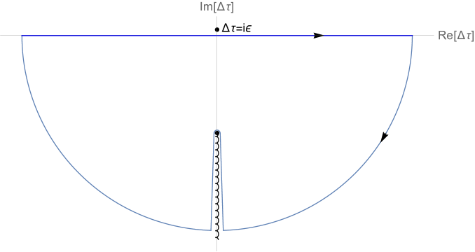
Figure 1: The complex contour used to obtain the detector excitation rate in Eq. (3.16), which shows that the integral over the real axis can be replaced by the two sections along the cut in the lower complex $\Delta u-$plane.

One can make use of the Cauchy integral formula to replace the integral in Eq. (3.30) by an equivalent integral,

$${\cal R}(\Delta E)\!\! = \!\!\frac{\hbar m\sqrt{\gamma}}{2\pi^{2}}\int_{\theta_{0}}^{\infty}\frac{{\rm d}\theta}{\big{[}h^{2}\sinh^{2}(\theta)-\theta^{2}\big{]}^{1/2}}{\rm e}^{-\frac{\Delta E}{P_{v}\omega_{g}}\theta}K_{1}\big{(}\frac{m}{P_{v}\omega_{g}}\theta\big{)}\,,\qquad$$ (3.33)

where we set $D=4$, which is allowed as the integral in Eq. (3.33) is finite in $D=4$, and therefore it does not need to be regularized. The parameter $\theta_{0}>0$ in Eq. (3.33) is the positive root of Eq. (3.32), we made use of the fact that the integral over the entire contour in figure 1 vanishes and, in the last step, made the replacement, $\theta\rightarrow-\theta$. In the massless limit Eq. (3.33) reduces to,

$${\cal R}(\Delta E)\!\! = \!\!\frac{\hbar\sqrt{\gamma}P_{v}\omega_{g}}{2\pi^{2}}\int_{\theta_{0}}^{\infty}\frac{{\rm d}\theta}{\theta\big{[}h^{2}\sinh^{2}(\theta)-\theta^{2}\big{]}^{1/2}}{\rm e}^{-\frac{\Delta E}{P_{v}\omega_{g}}\theta}\,.\qquad$$ (3.34)

The integrals in Eqs. (3.33–3.34) are hard, and cannot be evaluated analytically. Let us firstly consider the easier, massless case.

Two analytic approximations can be used for the transition rate in Eq. (3.30), an expansion in powers of $h^{2}$ and an expansion around the beginning of the cut, the latter increasing in accuracy in the large energy limit, when $\Delta E\gg P_{v}\omega_{g}$. The first approximation amounts to setting $D=4$ and expanding (3.30) in powers of $h^{2}$. This replaces the cut contribution by a sum over the poles at $\Delta u=i\epsilon$ of the order $2n+2$,

$${\cal R}(\Delta E)\!\! = \!\!\frac{\hbar m^{2}\sqrt{\gamma}}{4\pi^{2}}\frac{1}{\sqrt{\pi}}\sum_{n=1}^{\infty}\Gamma\big{(}n\!+\!\frac{1}{2}\big{)}\frac{h^{2n}}{n!}\!\int_{-\infty}^{\infty}\!\frac{{\rm d}\Delta\tau}{(P_{v}\omega_{g}\Delta\tau)^{2n}}\sin^{2n}(P_{v}\omega_{g}\Delta\tau){\rm e}^{-i\Delta E\Delta\tau}\frac{K_{1}\big{(}im(\Delta\tau\!-\!i\epsilon)\big{)}}{im(\Delta\tau\!-\!i\epsilon)},\qquad\;\;\;$$ (3.35)

which can be evaluated by making use of the Cauchy integral formula. The integration of the $n$th term in the sum does not vanish provided $\Delta E-2nP_{v}\omega_{g}<0$. In the massless limit the last term in Eq. (3.30) simplifies to, $-1/[m(\Delta\tau-i\epsilon)]^{2}$, such that the integral evaluates to,

$${\cal R}(\Delta E)\!\! = \!\!\frac{\hbar\sqrt{\gamma}P_{v}\omega_{g}}{2\pi^{2}}\Bigg{\{}\frac{\pi}{6}h^{2}\!\left(\!1\!-\!\frac{\Delta E}{2P_{v}\omega_{g}}\right)^{3}\!\Theta(2P_{v}\omega_{g}\!-\!\Delta E)$$

$$+ \!\!\frac{\pi}{5}h^{4}\left[-\frac{1}{8}\left(\!1\!-\!\frac{\Delta E}{2P_{v}\omega_{g}}\right)^{3}\!\Theta(2P_{v}\omega_{g}\!-\!\Delta E)\!+\!\left(\!1\!-\!\frac{\Delta E}{4P_{v}\omega_{g}}\right)^{3}\!\Theta(4P_{v}\omega_{g}\!-\!\Delta E)\right]\!+\!{\cal O}(h^{6})\Bigg{\}}\,,\qquad$$

where we made use of, $\sin^{2}(z)=\frac{1}{2}-\frac{1}{4}\left({\rm e}^{2iz}+{\rm e}^{-2iz}\right)$, and we have assumed that, $\Delta E>0$ and $P_{v}>0$.

The second analytic approximation can be obtained by expanding the integrand in Eq. (3.34) around the beginning of the cut. The result is,

$${\cal R}(\Delta E)\!\! \approx \!\!\frac{\hbar\sqrt{\gamma}P_{v}\omega_{g}}{2\pi^{2}}\sqrt{\frac{P_{v}\omega_{g}}{\Delta E}}\left(\frac{h}{2}\right)^{\frac{\Delta E}{P_{v}\omega_{g}}}\frac{1}{\left[\ln\left(\frac{2}{h}\right)+\ln\left(\ln\left(\frac{2}{h}\right)\right)\right]^{2+\frac{\Delta E}{P_{v}\omega_{g}}}}\left[1+{\cal O}\left(\frac{P_{v}\omega_{g}}{\Delta E}\right)\right]\,.\qquad$$ (3.37)

One can evaluate Eq. (3.34) numerically, and the results are shown in figure 2.

         

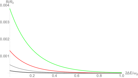
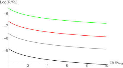
Figure 2: Left panel: The transition rate ${\cal R}$ in Eq. (3.34) for a massless scalar as a function of $\Delta E/(P_{v}\omega_{g})$ in units of ${\cal R}_{0}=\hbar\sqrt{1-h^{2}}P_{v}\omega_{g}/(2\pi^{2})$ as measured by the Unruh-DeWitt detector. Different curves are for different values of the gravitational strain (from top down): $h=0.1$ (green), $h=0.05$ (red), $h=0.025$ (gray), and $h=0.01$ (black). Right panel: The same diagram for $\ln({\cal R}/{\cal R}_{0})+\Delta E\theta_{0}/(P_{v}\omega_{g})$, where $\theta_{0}>0$ is the imaginary pole at the beginning of the square root cut in Eq. (3.31).

which probe different spatial gravitational potential induced by the gravitational backreaction from gravitational waves, and it is therefore purely quantum.The effect originates from the quantum interference between propagation on off-shell detector’s trajectories which probe different spatial gravitational potential induced by the gravitational backreaction from gravitational waves, and it is therefore purely quantum. In figure 3 we compare the numerical results for the transition rate with two analytical approximations. The first approximation is obtained by expanding in powers of $h^{2}$ (dashed lines in figure 3) and the second by expanding around the beginning of the cut (dotted lines in figure 3). Both approximations are reasonable, but neither is accurate. The second approximation captures correctly the large $\Delta E$ behavior, ${\cal R}(\Delta E)\propto{\rm exp}\left[-\frac{\Delta E}{P_{v}\omega_{g}}\theta_{0}\right]$, meaning that the transition rate is exponentially suppressed with growing $\left[\frac{\Delta E}{P_{v}\omega_{g}}\theta_{0}\right]$, but the analytical estimate poorly approximates the constant in front of the exponential. Due to the complicated dependence of $\theta_{0}(h)$ on $h$ in Eq. (3.32), the dependence of the transition rate on $h$ is nonanalytic, which explains why expanding in powers of $h^{2}$ performs relatively poorly. This kind of nonanalytic behavior is hard to guess, and impossible to obtain without knowing the scalar Wightman function from Ref. [1], which resums the gravitational wave insertions.

 

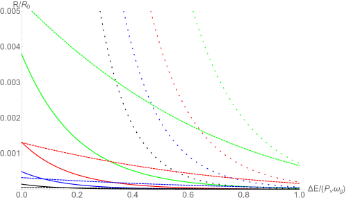
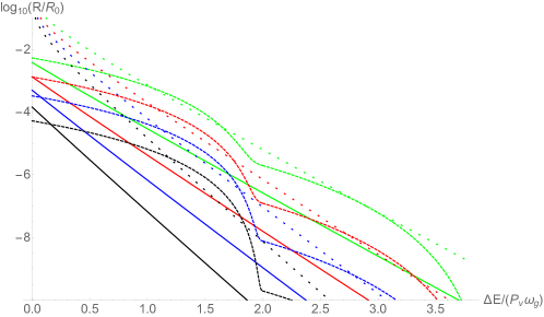
Figure 3: Left panel: The detector transition rate ${\cal R}$ for a massless scalar as a function of $\Delta E/(P_{v}\omega_{g})$ in units of ${\cal R}_{0}=\hbar\sqrt{1-h^{2}}P_{v}\omega_{g}/(2\pi^{2})$ as measured by the Unruh-DeWitt detector. Different curves are for different values of the gravitational strain: $h=0.1$ (green), $h=0.05$ (red), $h=0.025$ (blue), and $h=0.01$ (black). Solid lines show numerical results, dashed lines are approximate curves in Eq. (3), obtained by expanding the integrand in powers of $h^{2}$, and dotted lines represent the function in Eq. (3.37), obtained by expanding the integrand around the beginning of the cut. Right panel: The same diagram for $\log_{10}({\cal R}/{\cal R}_{0})$.

The effect originates from the quantum interference between propagation on off-shell detector’s trajectories which probe different spatial gravitational potential induced by the gravitational backreaction from gravitational waves, and it is therefore purely quantum.

Switching on the scalar mass suppresses the transition rate further, and the results obtained by numerically integrating (3.33) for $m=P_{v}\omega_{g}$ shown in figure 4 are significantly suppressed when compared with those for the massless scalar in figures 2 and 3.

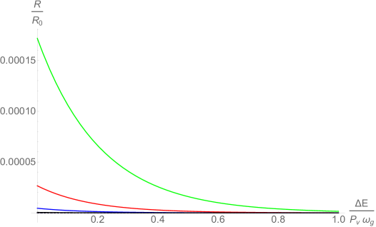
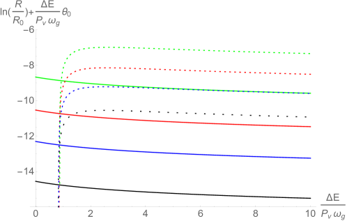
Figure 4: Left panel: The detector transition rate ${\cal R}(\Delta E)$ for a massive scalar with $m=P_{v}\omega_{g}$ as a function of $\Delta E/(P_{v}\omega_{g})$ in units of ${\cal R}_{0}=\hbar\sqrt{1-h^{2}}P_{v}\omega_{g}/(2\pi^{2})$ as measured by the Unruh-DeWitt detector. Different curves are for different values of the gravitational strain: $h=0.1$ (green), $h=0.05$ (red), $h=0.025$ (blue), and $h=0.01$ (black). Right panel: The same diagram for $\ln({\cal R}/{\cal R}_{0})+(\Delta E\theta_{0})/(P_{v}\omega_{g})$.

Just as in the massless case, at large $\Delta E$, the results decay exponentially as, ${\cal R}\propto\exp\left[-\frac{\Delta E}{P_{v}\omega_{g}}\theta_{0}\right]$, and in the limit of a large mass, $m\theta_{0}\gg P_{v}\omega_{g}$, there is an additional exponential suppression, ${\cal R}\propto\exp\left[-\frac{(\Delta E+m)}{P_{v}\omega_{g}}\theta_{0}\right]$. To see that, let us approximately evaluate the integral in Eq. (3.33) by expanding around the beginning of the cut at $\theta=\theta_{0}(h)$,

$${\cal R}(\Delta E)\!\! = \!\!\frac{\hbar\sqrt{\gamma}m}{2\pi^{2}}\sqrt{\frac{\pi P_{v}\omega_{g}}{2\Delta E\theta_{0}(\theta_{0}-1)}}K_{1}\left(\frac{m\theta_{0}}{P_{v}\omega_{g}}\right){\rm e}^{-\frac{\Delta E\theta_{0}}{P_{v}\omega_{g}}}$$ (3.38)

$$\times \!\!\Bigg{\{}1-\frac{P_{v}\omega_{g}}{2\Delta E}\Bigg{[}\frac{2\theta_{0}^{2}-1}{4\theta_{0}(\theta_{0}-1)}+\frac{m}{P_{v}\omega_{g}}\frac{K_{2}\left(\frac{m\theta_{0}}{P_{v}\omega_{g}}\right)}{K_{1}\left(\frac{m\theta_{0}}{P_{v}\omega_{g}}\right)}-\frac{1}{\theta_{0}}\Bigg{]}+{\cal O}(\Delta E^{-2})\Bigg{\}}\,,\qquad$$

which applies when $\Delta E\theta_{0}/(P_{v}\omega_{g})\gg 1$, and where we dropped the term $h^{2}/(2\theta_{0})$ in the expansion, $\sqrt{\theta_{0}^{2}+h^{2}}\simeq\theta_{0}+{\cal O}(h^{2}/\theta_{0})$. This amounts to approximating the position of the cut, $\theta=\theta_{0}(h)$, by the Lambert function in Eq. (3.32). We shall not attempt to evaluate the integrals in Eq. (3.35) for the massive case, as that would require not only to account for the contributions of the poles at $\Delta u=i\epsilon$, but also for the contribution of the logarithmic cut of the modified Bessel function, $im(\Delta u-i\epsilon)K_{1}\big{(}im(\Delta u-i\epsilon)\big{)}$, which extends from $\Delta u=0$ to $0+i\infty$. Finally, in figure 5 we show the same transition rate as in figure 4, but now as a function of the mass for a fixed $\Delta E=2P_{v}\omega_{g}$ (left panel) and $\Delta E=10P_{v}\omega_{g}$ (right panel). The figure shows that the transition rate is exponentially suppressed by the mass as, ${\cal R}\sim{\rm e}^{-m\theta_{0}(h)/(P_{v}\omega_{g})}$, which can be also inferred from the asymptotic expansion of the Bessel function in Eq. (3.38), $K_{1}\left(\frac{m\theta_{0}}{P_{v}\omega_{g}}\right)\sim\sqrt{\frac{\pi P_{v}\omega_{g}}{2m\theta_{0}}}\exp\left(-\frac{m\theta_{0}}{P_{v}\omega_{g}}\right)$.

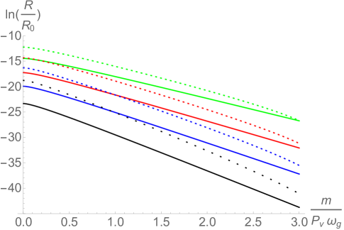
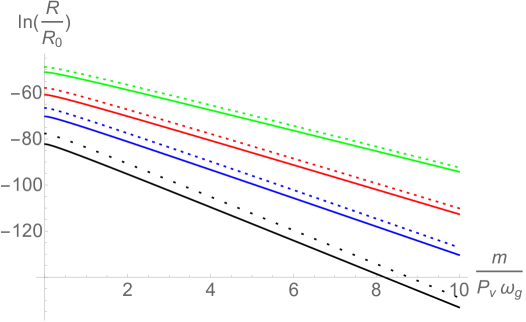
Figure 5: Left panel: The detector transition rate ${\cal R}$ for a massive scalar with $\Delta E/(P_{v}\omega_{g})=2$ as a function of $m/(P_{v}\omega_{g})$ in units of ${\cal R}_{0}=\hbar\sqrt{1-h^{2}}P_{v}\omega_{g}/(2\pi^{2})$ as measured by the Unruh-DeWitt detector. Different curves are for different values of the gravitational strain: $h=0.1$ (green), $h=0.05$ (red), $h=0.025$ (blue), and $h=0.01$ (black). Right panel: The same but with with $\Delta E/(P_{v}\omega_{g})=10$. The solid curves are numerical results, and the short dashed curves are the approximation in Eq. (3.38).

Monochromatic elliptically polarized gravitational waves. Here we shall consider general elliptically polarized gravitational waves, whose analysis is much trickier, as the interaction with the detector depends on the average time variable, $U=(u+u^{\prime})/2$. Let us begin our analysis by noting that Eq. (2.26) can be recast as,

$${\cal G}^{ij}(U,\Delta u)=\sum_{n=0}^{\infty}\left[\frac{\partial^{2n}}{\partial U^{2n}}g^{ij}(U)\right]\frac{\left({\Delta u}/{2}\right)^{2n}}{(2n+1)!}\,,\qquad$$ (3.39)

where $\Delta u=u\!-\!u^{\prime}$, and $g^{ij}(U)$ denotes the inverse of $g_{ij}(U)$, which for generally polarized waves (fluctuating in a 2-dimensional plane) takes the form (cf. Eq. (2.32)),

$$g^{ij}(U)\!\! = \!\!\frac{1}{1-h_{+}^{2}c_{+}^{2}-h_{\times}^{2}c_{\times}^{2}}\left(\!\!\begin{array}[]{cc}1-h_{+}c_{+}&-h_{\times}c_{\times}\cr-h_{\times}c_{\times}&1+h_{+}c_{+}\cr\end{array}\!\!\right)\,,\qquad$$ (3.42)

where $c_{+}(U)=\cos(\omega_{g}U+\psi/2)$, $c_{\times}(U)=\cos(\omega_{g}U-\psi/2)$, where $\psi$ is an arbitrary phase (in the case of nonpolarized gravitational waves, $\psi=\pi/2$). Evaluating (3.39) for $g^{ij}$ in Eq. (3.42) is a formidable task, and we shall content ourselves by evaluating ${\cal G}^{ij}(u;u^{\prime})$ to the quadratic order in $h_{+}$ and $h_{\times}$,

$${\cal G}^{ij}(U,\Delta u)\!\! = \!\!\left(\!\!\begin{array}[]{cc}1&0\cr 0&1\cr\end{array}\!\!\right)\left[1+\frac{h_{+}^{2}}{2}\left(1+(2c_{+}^{2}-1)j_{0}(\omega_{g}\Delta u)\right)+\frac{h_{\times}^{2}}{2}\left(1+(2c_{\times}^{2}-1)j_{0}(\omega_{g}\Delta u)\right)\right]$$ (3.48)

$$\!\!+\,\left(\!\!\begin{array}[]{cc}-h_{+}c_{+}&-h_{\times}c_{\times}\cr-h_{\times}c_{\times}&h_{+}c_{+}\cr\end{array}\!\!\right)j_{0}\left(\frac{\omega_{g}\Delta u}{2}\right)+{\cal O}(h_{+}^{2}h_{\times},h_{+}h_{\times}^{2})\,,\qquad$$

whose determinant equals,

$${\cal G}^{-1}(U;\Delta u)\!\! = \!\!1-h_{+}^{2}\left[c_{+}^{2}j_{0}^{2}\left(\frac{\omega_{g}\Delta u}{2}\right)-1-(2c_{+}^{2}-1)j_{0}(\omega_{g}\Delta u)\right]\qquad\quad$$ (3.49)

$$- \!\!h_{\times}^{2}\left[c_{\times}^{2}j_{0}^{2}\left(\frac{\omega_{g}\Delta u}{2}\right)-1-(2c_{\times}^{2}-1)j_{0}(\omega_{g}\Delta u)\right]+{\cal O}(h_{+}^{2}h_{\times},h_{+}h_{\times}^{2})\,.\qquad$$

In the circularly polarized case, in which $\psi=\pi/2$ and $h_{+}=h_{\times}=h$, this reduces to, ${\cal G}^{-1}(U;\Delta u)\rightarrow 1-h^{2}\left[j_{0}^{2}\left(\frac{\omega_{g}\Delta u}{2}\right)+2\right]$, which agrees with Eq. (3.29) when one recalls that, $1/\gamma^{2}=1+2h^{2}+{\cal O}(h^{4})$. Upon introducing $\tilde{\gamma}(h_{+},h_{\times})=1-\frac{h_{+}^{2}+h_{\times}^{2}}{2}$, Eq. (3.49) can be recast as,

$${\cal G}^{-1}(U;\Delta u)\!\! = \!\!\frac{1}{\tilde{\gamma}^{2}}\left\{1-\left[\big{(}h_{+}^{2}c_{+}^{2}+h_{\times}^{2}c_{\times}^{2}\big{)}j_{0}^{2}\left(\frac{\omega_{g}\Delta u}{2}\right)-\big{(}h_{+}^{2}(2c_{+}^{2}-1)+h_{\times}^{2}(2c_{\times}^{2}-1)\big{)}j_{0}(\omega_{g}\Delta u)\right]\right\}\qquad\;$$ (3.50)

$$\!\!+\,{\cal O}(h_{+}^{2}h_{\times},h_{+}h_{\times}^{2})\,.\qquad$$

To complete the analysis, we also need,

$$\sqrt{\gamma(u)\gamma(u^{\prime})}=\tilde{\gamma}-\frac{1}{2}\left(h_{+}^{2}(2c_{+}^{2}-1)+h_{\times}^{2}(2c_{\times}^{2}-1)\right)\cos(\omega_{g}\Delta u)+\,{\cal O}(h_{+}^{2}h_{\times},h_{+}h_{\times}^{2})\,,\qquad$$ (3.51)

which, when multiplied with (3.50), gives,

$$\sqrt{\gamma(u)\gamma(u^{\prime})}{\cal G}^{-1}(U;\Delta u)\!\! = \!\!\frac{1}{\tilde{\gamma}}\bigg{\{}1-\bigg{[}\big{(}h_{+}^{2}c_{+}^{2}+h_{\times}^{2}c_{\times}^{2}\big{)}j_{0}^{2}\left(\frac{\omega_{g}\Delta u}{2}\right)$$

$$\!\!\hskip-56.9055pt-\,\big{(}h_{+}^{2}(2c_{+}^{2}-1)+h_{\times}^{2}(2c_{\times}^{2}-1)\big{)}\Big{(}j_{0}(\omega_{g}\Delta u)-\frac{1}{2}\cos(\omega_{g}\Delta u)\Big{)}\bigg{]}\bigg{\}}+\,{\cal O}(h_{+}^{2}h_{\times},h_{+}h_{\times}^{2})\,.\qquad$$

This product appears in the propagator in Eq. (3.22), and generates square-root cuts , just as in the circularly polarized waves in Eq. (3.30). The integral can be evaluated by contour integration, with the contour showed in figure 1, resulting in the cut contribution (cf. Eq. (3.33)),

$${\cal R}(U,\Delta E)\!\! = \!\!\frac{\hbar m\sqrt{\tilde{\gamma}}}{2\pi^{2}}\int_{\theta_{0}}^{\infty}\frac{{\rm d}\theta}{\big{[}H^{2}(U,\theta)-\theta^{2}\big{]}^{1/2}}{\rm e}^{-\frac{\Delta E}{P_{v}\omega_{g}}\theta}K_{1}\big{(}\frac{m}{P_{v}\omega_{g}}\theta\big{)}\,,\qquad$$ (3.53)

where $h^{2}(U)=h_{+}^{2}c_{+}^{2}(U)+h_{\times}^{2}c_{\times}^{2}(U)$,

$$H^{2}(U,\theta)=h^{2}(U)\sinh^{2}(\theta)+\Big{[}h^{2}(U)-\frac{h_{+}^{2}+h_{\times}^{2}}{2}\Big{]}\Big{[}\theta^{2}\cosh(2\theta)-\theta\sinh(2\theta)\Big{]}\,,\qquad\;$$ (3.54)

and $\theta_{0}>0$ denotes the beginning of the cut defined by, $H^{2}(U,\theta_{0})=\theta_{0}^{2}$. Next we insert,

$$h^{2}(U)=\frac{h_{+}^{2}\!+\!h_{\times}^{2}}{2}+\frac{h_{+}^{2}\!+\!h_{\times}^{2}}{2}\cos(2\omega_{g}U)c_{\psi}-\frac{h_{+}^{2}\!-\!h_{\times}^{2}}{2}\sin(2\omega_{g}U)s_{\psi},\quad\big{(}c_{\psi}=\cos(\psi),\;s_{\psi}=\sin(\psi)\big{)},\;$$ (3.55)

into Eq. (3.54) to obtain,

$$\bigg{[}\frac{h_{+}^{2}\!+\!h_{\times}^{2}}{2}c_{\psi}\cos(2\omega_{g}U)-\frac{h_{+}^{2}\!-\!h_{\times}^{2}}{2}s_{\psi}\sin(2\omega_{g}U)\bigg{]}\Big{[}\sinh^{2}(\theta_{0})+\theta_{0}^{2}\cosh(2\theta_{0})-\theta_{0}\sinh(2\theta_{0})\Big{]}$$

$$\hskip 284.52756pt+\,\frac{h_{+}^{2}+h_{\times}^{2}}{2}\sinh^{2}(\theta_{0})-\theta_{0}^{2}=0\,.\qquad$$ (3.56)

Because of the $U$ dependence, Eq. (3.56) may or may not have a solution, meaning that the cuts exist only when (3.56) can be solved for some real $U$. To simplify our analysis, recall that we are interested in the limit when, $h_{+},h_{\times}\ll 1$, in which case in most of the parameter space $\theta_{0}\gg 1$, and one can approximate Eq. (3.56) by keeping the leading order terms $\propto{\rm e}^{2\theta_{0}}$ only.  Multiplying Eq. (3.56) by $2{\rm e}^{-2\theta_{0}}/\cos^{2}(\omega_{g}U)=2{\rm e}^{-2\theta_{0}}(1+t^{2})$ and neglecting the terms suppressed as $\sim{\rm e}^{-2n\theta_{0}}\;(n=1,2)$ yields a quadratic equation for $t=\tan(\omega_{g}U)$,

$$at^{2}-2bt+c>0\;\Longrightarrow\;a(t-t_{+})(t-t_{-})>0,\quad t_{\pm}=\frac{1}{a}\big{[}b\pm\sqrt{\Delta}\big{]}\,,\qquad\Delta=b^{2}-ac,\;$$ (3.57)

where

$$a=\frac{h_{+}^{2}\!+\!h_{\times}^{2}}{2}\left[-\Big{(}\!\theta_{0}^{2}\!-\!\theta_{0}+\frac{1}{2}\Big{)}c_{\psi}\!+\!\frac{1}{2}\right],\quad b=\frac{h_{+}^{2}\!-\!h_{\times}^{2}}{2}\Big{(}\!\theta_{0}^{2}\!-\!\theta_{0}\!+\!\frac{1}{2}\Big{)}s_{\psi},\quad c=\frac{h_{+}^{2}\!+\!h_{\times}^{2}}{2}\left[\Big{(}\!\theta_{0}^{2}\!-\!\theta_{0}+\frac{1}{2}\Big{)}c_{\psi}\!-\!\frac{1}{2}\right],$$ (3.58)

and we made use of, $\cos(2\omega_{g}U)=(1-t^{2})/(1+t^{2})$ and $\sin(2\omega_{g}U)=2t/(1+t^{2})$. The discriminant in Eq. (3.57) is then,

$$\Delta\!\! = \!\!\left(\frac{h_{+}^{2}\!+\!h_{\times}^{2}}{2}\right)^{2}\left[\Big{(}\!\theta_{0}^{2}\!-\!\theta_{0}+\frac{1}{2}\Big{)}^{2}\!-\!\frac{1}{4}\right]\!-\!h_{+}^{2}h_{\times}^{2}\Big{(}\!\theta_{0}^{2}\!-\!\theta_{0}\!+\!\frac{1}{2}\Big{)}^{2}s^{2}_{\psi}$$ (3.59)

$$= \!\!\left(\frac{h_{+}^{2}\!-\!h_{\times}^{2}}{2}\right)^{2}\left[\Big{(}\!\theta_{0}^{2}\!-\!\theta_{0}+\frac{1}{2}\Big{)}^{2}\!-\!\frac{1}{4}\right]\!+\!h_{+}^{2}h_{\times}^{2}\left[\Big{(}\!\theta_{0}^{2}\!-\!\theta_{0}\!+\!\frac{1}{2}\Big{)}^{2}c^{2}_{\psi}\!-\!\frac{1}{4}\right]\,.\qquad\;$$

The roots $t_{\pm}$ in Eq. (3.57) of the equation, $at^{2}-2bt+c=0$, are real if $\Delta\geq 0$, from which we conclude that the inequality in Eq. (3.57) is satisfied:

1. when $a>0$ and $\Delta<0$: the inequality in Eq. (3.57) is satisfied for all $U\in{\mathbb{R}}$;

2. when $a>0$ and $\Delta\geq 0$: the inequality in Eq. (3.57) is satisfied for $t=\tan(\omega_{g}U)<t_{-}$ and $\tan(\omega_{g}U)>t_{+}$;

3. when $a<0$ and $\Delta\geq 0$: the inequality in Eq. (3.57) is satisfied for $t_{-}<\tan(\omega_{g}U)<t_{+}$;

4. when $a<0$ and $\Delta<0$: the inequality in Eq. (3.57) is never satisfied.

From Eqs. (3.58) and (3.59) we then see that $a\lessgtr 0$ and $\Delta{\geq\atop<}$ imply,

$$\cos(\psi)\!\! \lessgtr \!\!\frac{1}{2\theta_{0}(\theta_{0}-1)+1}\simeq\frac{1}{2\theta_{0}^{2}}$$ (3.60)

$$\cos^{2}(\psi)\!\! {\geq\atop<} \!\!\frac{1}{[2\theta_{0}(\theta_{0}-1)+1]^{2}}-\frac{1}{4}\left(\frac{h_{+}}{h_{\times}}\!-\!\frac{h_{\times}}{h_{+}}\right)^{2}\left[1-\frac{1}{[2\theta_{0}(\theta_{0}-1)+1]^{2}}\right]\simeq\frac{1}{4\theta_{0}^{4}}-\frac{1}{4}\left(\frac{h_{+}}{h_{\times}}\!-\!\frac{h_{\times}}{h_{+}}\right)^{\!2},\qquad$$

where the last inequalities represent good approximations when $\theta_{0}\gg 1$. Notice that if,

$$\left|\frac{h_{+}}{h_{\times}}\!-\!\frac{h_{\times}}{h_{+}}\right|>\frac{1}{\sqrt{\theta_{0}(\theta_{0}-1)(\theta_{0}^{2}-\theta_{0}+1)}}\simeq\frac{1}{\theta_{0}(\theta_{0}-1)}\;\Longrightarrow\Delta>0\,,$$ (3.61)

and options (1) and (4) are absent, and an Unruh-DeWitt detector gets excited only during parts of the period. For circularly polarized gravitational waves, $\cos(\psi)=0$, and excitations occur when,

$$t_{-}<\tan(\omega_{g}U)<t_{+}\,.$$ (3.62)

There is another important difference between detector’s transition rate induced by circularly polarized and elliptically polarized gravitational waves. Upon rewriting Eq. (3.56) at leading order in ${\rm e}^{2\theta_{0}}$,

$$\frac{h_{+}^{2}\!+\!h_{\times}^{2}}{2}\!+\!\bigg{[}\frac{h_{+}^{2}\!+\!h_{\times}^{2}}{2}c_{\psi}\cos(2\omega_{g}U)\!-\!\frac{h_{+}^{2}\!-\!h_{\times}^{2}}{2}s_{\psi}\sin(2\omega_{g}U)\bigg{]}\Big{[}2\theta_{0}(\theta_{0}\!-\!1)\!+\!1\Big{]}\!+\!{\cal O}\left({\rm e}^{-2\theta_{0}}\right)=4\theta_{0}^{2}{\rm e}^{-2\theta_{0}}\,,\qquad$$ (3.63)

we see that only the first term in Eq. (3.63) survives in the circularly polarized case, in which $h_{+}=h_{\times}$ and $\cos(\psi)=0$. Very close to that point, the first term $(h_{+}^{2}\!+\!h_{\times}^{2})/{2}$ dominates, and the beginning of the cut is still well approximated in terms of the Lambert function as (cf. Eq. (3.32)),

$$\theta_{0}(h_{+},h_{\times})\simeq-\Re\bigg{[}W\bigg{(}\!\!-\frac{1}{2}\sqrt{\frac{h_{+}^{2}+h_{\times}^{2}}{2}}\,\bigg{)}\bigg{]}\,,$$ (3.64)

whose small $\bar{h}\equiv\sqrt{(h_{+}^{2}+h_{\times}^{2})/2}-$expansion is highly nonanalytic. On the other hand, when deviations from the circularly polarized case are significant, the solution changes to,

$$\theta_{0}(h_{+},h_{\times})\simeq-\frac{1}{2}\ln\bigg{[}\frac{h_{+}^{2}\!+\!h_{\times}^{2}}{4}c_{\psi}\cos(2\omega_{g}U)\!-\!\frac{h_{+}^{2}\!-\!h_{\times}^{2}}{4}s_{\psi}\sin(2\omega_{g}U)\bigg{]}\,,$$ (3.65)

which exists when the argument of the logarithm is positive, i.e. when $\tan(2\omega_{g}U)\lessgtr\Big{(}\frac{h_{+}^{2}+h_{\times}^{2}}{h_{+}^{2}-h_{\times}^{2}}\Big{)}\cot(\psi)$ for $(h_{+}^{2}-h_{\times}^{2})\sin(\psi)\lessgtr 0$.

With these considerations in mind, one can obtain an approximate expression for the detector rate in the massless limit (cf. Eq. (3.37)),

$${\cal R}(U,\Delta E)\!\! \approx \!\!\frac{\hbar\sqrt{\tilde{\gamma}}P_{v}\omega_{g}}{2\pi^{2}}\sqrt{\frac{P_{v}\omega_{g}}{\Delta E}}\left(\frac{h_{+}^{2}c_{+}^{2}(U)\!+\!h_{\times}^{2}c_{\times}^{2}(U)}{2}\!-\!\frac{h_{+}^{2}\!+\!h_{\times}^{2}}{4}\right)^{\frac{\Delta E}{2P_{v}\omega_{g}}}\Theta_{+}\,,\qquad$$ (3.66)

where $\Theta_{+}=1$ when the argument inside the brackets is positive (which is identical the positivity requirement on the argument of the logarithm in Eq. (3.65)), and $\Theta_{+}=0$ when it is negative. A second perturbative approximation can be obtained by expanding the integrand in Eq. (3.22) in powers of the gravitational strain. Making use of Eq. (3) and keeping, for simplicity, the quadratic order terms only, one obtains for the detector’s transition rate in the massless scalar case,

$${\cal R}(\Delta E)\!\! = \!\!\frac{\hbar\sqrt{\tilde{\gamma}}P_{v}\omega_{g}}{2\pi}\Bigg{\{}\frac{h^{2}(U)}{6}\!\left(\!1\!-\!\frac{\Delta E}{2P_{v}\omega_{g}}\right)^{3}\!\!+\!\frac{2h^{2}(U)\!-\!(h_{+}^{2}\!+\!h_{\times}^{2})}{4}\!\left(\!1\!-\!\frac{\Delta E}{2P_{v}\omega_{g}}\right)\frac{\Delta E}{2P_{v}\omega_{g}}\Bigg{\}}\Theta(2P_{v}\omega_{g}\!-\!\Delta E)$$ (3.67)

$$+ \!\!{\cal O}(h_{+,\times}^{4})\,,\qquad$$

where $h^{2}(U)=h_{+}^{2}c_{+}^{2}(U)+h_{\times}^{2}c_{\times}^{2}(U)$, and we have dropped the quartic terms as they are significantly more complicated than in the circularly polarized case in Eq. (3).

In figure 6 we show selected numerical results of integrating Eq. (3.53) in the massless limit, in which the transition rate reduces to (cf. Eq. (3.34)),

$${\cal R}(\Delta E)\!\! = \!\!\frac{\hbar\sqrt{\tilde{\gamma}}P_{v}\omega_{g}}{2\pi^{2}}\int_{\theta_{0}}^{\infty}\frac{{\rm d}\theta}{\theta\big{[}H^{2}(U,\theta)-\theta^{2}\big{]}^{1/2}}{\rm e}^{-\frac{\Delta E}{P_{v}\omega_{g}}\theta}\,.\qquad$$ (3.68)

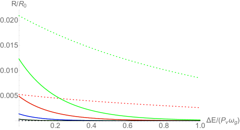
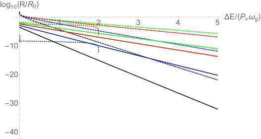
Figure 6: Left panel: The detector’s transition rate ${\cal R}$ for a massless scalar as a function of $\Delta E/(P_{v}\omega_{g})$ in units of ${\cal R}_{0}=\hbar\sqrt{\tilde{\gamma}}P_{v}\omega_{g}/(2\pi^{2})$ as measured by a freely falling Unruh-DeWitt detector. All curves are for the moment in time, $U=\pi/4\omega_{g}$ and for the relative phase, $\psi=\pi/2$, which is the same phase difference as for circularly polarized waves. Different curves are for different values of the gravitational strains: $h_{+}=0.1$ and $h_{\times}=0.2$ (green), $h_{+}=0.01$ and $h_{\times}=0.1$ (red), $h_{+}=0.01$ and $h_{\times}=0.001$ (blue), and $h_{+}=0$ and $h_{\times}=0.0001$ (black). Right panel: The same but now for $\log_{10}[{\cal R}/{\cal R}_{0}]$. The solid curves are numerical results, the dashed curves are obtained by using the approximation in Eq. (3.66), and the dotted lines correspond to the approximation in Eq. (3.67).

In the same figure, for comparison, we also show the analytical estimates from Eq. (3.66) (dashed) and from Eq. (3.67) (dotted). Notice that the latter approximation (obtained by expanding in powers of $h$) does not work as well as in the circularly polarized case, as it does not need to give a positive result in the whole interval, $0\leq\Delta E\leq 2P_{v}\omega_{g}$.  The detector’s transition rate for a massive scalar field can be studied analogously, and therefore we leave it as an exercise.

None of the results presented in this section can be compared with those in Ref. [9], where approximations were used which do not capture the effects of the cuts in figure 1. 

4 Conclusions and outlook

In section 2 we generalize the massive real scalar field propagator of Ref. [1] to general gravitational waves propagating in one direction, thus relaxing the monochromatic approximation used in Ref. [1]. The Wightman two-point functions are given in Eq. (2.4) and the propagator in Eqs. (2.39–2.40). We then show that the generalized propagator produces the one-loop results which are identical in form to the ones obtained in Ref. [1].

In section 3 we then study how a freely falling Unruh-DeWitt detector (which couples to a massless or massive scalar field) responds to the gravitational wave background. We find that the deformation of the invariant distance induced by the gravitational waves gets fully compensated by the motion of a freely falling detector, thus leaving the effect of the modified amplitude of vacuum fluctuations expressed by the $(u,u^{\prime})-$dependent prefactor in Eq. (2.4), the effects of which we study in some detail. In this work we focus on studying detector’s excitation rate induced by passing gravitational waves, i.e. the rate of transitions from the detector’s ground state (with energy $E_{0}$) to an excited state $E$, for which $\Delta E=E-E_{0}>0$. These transitions are of a particular interest as they are completely absent in Minkowski space, and therefore – no matter how small it may be – any observed rate can be interpreted as the detection of gravitational waves.

We treat the detector’s transition rate in three different approximations:

1. Numerical solution, which can be considered to be exact. The resulting detector’s excitation rate ${\cal R}$ is exponentially suppressed, and can be approximated by, ${\cal R}={\cal R}_{0}(\Delta E,m,\omega_{g})\exp\left[-\frac{\Delta E}{P_{v}\omega_{g}}\theta_{0}(h)\right]$, where $\theta_{0}(h)>0$ is the beginning of the cut in the complex $\Delta u$ plane, whose functional dependence on $h$ is determined by Eq. (3.31), and it is highly nonanalytic; ${\cal R}_{0}(\Delta E,m,\omega_{g})$ is a weak function of $\Delta E/(P_{v}\omega_{g})$ and exponentially decays with increasing $m/(P_{v}\omega_{g})$.

2. Expanding in powers of $h^{2}$, where $h$ is the gravitational wave strain. This generates a series of poles of the order $2n+2$, each of which contributes to the term $\sim h^{2n}$ when $0\leq\Delta E\leq 2nP_{v}\omega_{g}$, the first two contributions are shown in Eq. (3) for circularly polarized gravitational waves and in Eq. (3.67) for general elliptically polarized gravitational waves.

   The field theoretic interpretation of these contributions is that they actively contribute when the scalar field absorbs $2n$ gravitons, each of which with energy $P_{v}\omega_{g}$, such that the detector’s energy can increase by $\Delta E\leq 2nP_{v}\omega_{g}$. Figures 3 and 6 show that expanding in powers of the gravitational wave strain captures correctly the qualitative trend of the numerical solution, but at the quantitative level this approximation performs quite poorly.

3. Expanding around the cut at $\theta=\theta_{0}(h)$ in Eqs. (3.31) and (3.56) for circularly polarized and elliptically polarized gravitational waves, respectively. The leading order result is shown in Eq. (3.37) for circularly polarized waves and in Eq. (3.66) for elliptically polarized waves. This approximation captures correctly the exponential decay of the detector’s excitation rate with increasing $\Delta E>0$, that is its nonanalytic structure in the gravitational wave strain, but it fails to correctly model the exponential prefactor, as can be clearly seen from figures 3, 4, 5 and 6.

In this work we have addressed the response of an Unruh-DeWitt detector to monochromatic, unidirectional, circularly polarized and elliptically polarized, gravitational waves. A more general investigation is warranted by relaxing any of the above mentioned restrictions. It would be, in particular, of interest to calculate the transition rate of the detector induced by a stochastic gravitational wave background. But to do that properly requires knowledge of the corresponding propagator, which is presently unknown.

5 Appendices

Appendix A: Derivation of the Wightman functions

Here we briefly present a derivation of the Wightman functions by the method of mode sums. Upon expanding the scalar field operator in terms of the momentum space mode functions $\phi_{\pm}(u,\vec{k})$ and the creation and annihilation operators $\hat{a}^{\dagger}(\vec{k})$ and $\hat{a}(\vec{k})$,

$$\hat{\phi}(u,\vec{x}_{\perp},v)\!\! = \!\!\int\frac{{\rm d}^{D-2}k_{\perp}{\rm d}k^{D-1}}{(2\pi)^{D-1}}{\rm e}^{i\vec{k}_{\perp}\cdot\vec{x}_{\perp}}\Big{[}{\rm e}^{-\frac{i}{2}\Omega_{-}(\vec{k}\,)v}\phi_{+}(u,\vec{k}\,)\hat{a}(\vec{k}\,)+{\rm e}^{\frac{i}{2}\Omega_{+}(\vec{k}\,)v}\phi_{-}(u,\vec{k}\,)\hat{a}^{\dagger}(-\vec{k}\,)\Big{]}\,,$$ (5.1)

which obey a standard non-vanishing commutation relation,

$$\left[\hat{a}(\vec{k}\,),\hat{a}^{\dagger}(\vec{k}^{\prime})\right]=(2\pi)^{D-1}\delta^{D-1}(\vec{k}\!-\!\vec{k}^{\prime})\,,$$

one obtains the following expressions for the positive and negative frequency Wightman functions,

$$i\Delta^{(+)}(x;x^{\prime})\!\! = \!\!\left\langle\Omega\right|\hat{\phi}(x)\hat{\phi}(x^{\prime})\left|\Omega\right\rangle=\int\!\frac{{\rm d}^{D-1}k}{(2\pi)^{D-1}}\,{\rm e}^{i\vec{k}_{\perp}\cdot\,\Delta\vec{x}_{\perp}-\frac{i}{2}\Omega_{-}(\vec{k})\Delta v}\phi_{+}(u,\vec{k}\,)\phi_{-}(u^{\prime},-\vec{k}\,)\,,$$ (5.2)

$$i\Delta^{(-)}(x;x^{\prime})\!\! = \!\!\left\langle\Omega\right|\hat{\phi}(x^{\prime})\hat{\phi}(x)\left|\Omega\right\rangle=\int\!\frac{{\rm d}^{D-1}k}{(2\pi)^{D-1}}\,{\rm e}^{i\vec{k}_{\perp}\cdot\,\Delta\vec{x}_{\perp}+\frac{i}{2}\Omega_{+}(\vec{k})\Delta v}\phi_{-}(u,\vec{k}\,)\phi_{+}(u^{\prime},-\vec{k}\,)$$ (5.3)

$$\hskip 85.35826pt=\,\int\!\frac{{\rm d}^{D-1}k}{(2\pi)^{D-1}}\,{\rm e}^{-i\vec{k}_{\perp}\cdot\,\Delta\vec{x}_{\perp}+\frac{i}{2}\Omega_{-}(\vec{k})\Delta v}\phi_{-}(u,-\vec{k}\,)\phi_{+}(u^{\prime},\vec{k}\,)\,,\qquad\;\;$$

where $\Delta\vec{x}_{\perp}=\vec{x}_{\perp}-\vec{x}_{\perp}^{\,\prime}$, $\Delta v=v\!-\!v^{\prime}$, and we have assumed,

$$\hat{a}(\vec{k}\,)|\Omega\rangle=0\,,\qquad(\forall\vec{k}\in{\mathbb{R}}^{D-1})\,.$$ (5.4)

The functions $\phi_{+}(u,\vec{k}\,)$ and $\phi_{-}(u^{\prime},\vec{k}\,)$ are the positive and negative frequency mode functions obeying,

$$\!\left(\!\partial_{u}\!\pm\!\frac{i}{2\Omega_{\mp}}\Big{[}\big{(}g^{ij}(u)-\delta^{ij}_{\perp}\big{)}k_{i}k_{j}\Big{]}\!\pm\!\frac{i}{2}\Omega_{\pm}\right)\!\big{[}\gamma^{1/4}(u)\phi_{\pm}(u,\vec{k})\big{]}=0,\hskip 5.69046pt$$ (5.5)

where $\Omega_{\pm}(\vec{k})=\omega\pm k^{D-1}$, $\gamma(u)={\rm det}[g_{ij}(u)]$, and $\omega=\sqrt{\|\vec{k}\|^{2}+m^{2}}$. This is a first order differential equation in $u$ and therefore can be easily solved. The properly normalized, ground state solutions of Eq. (5.5) are given by,

$$\phi_{\pm}(u,\vec{k})=\frac{1}{\gamma^{1/4}(u)}\sqrt{\frac{\hbar}{2\omega}}\exp\left[\mp\frac{i\Omega_{\pm}}{2}\left(u+\frac{k_{i}k_{j}}{\omega^{2}_{\perp}}\int^{u}{\rm d}\bar{u}\big{(}g^{ij}(\bar{u})-\delta^{ij}\big{)}\right)\right]\,,\qquad$$ (5.6)

where $\omega_{\perp}^{2}=\omega^{2}-(k^{D-1})^{2}$ and $\omega^{2}=\|\vec{k}\|^{2}+m^{2}$. The factor $\gamma^{-1/4}(u)$ in the normalization of the mode functions (5.6) can be traced back to the Wronskian condition for the mode functions (which in turn originates from canonical quantization). Together with the condition (5.4), the choice of pure positive (negative) frequency solutions for the functions $\phi_{+}$ ($\phi_{-}$) in Eq. (5.1) uniquely specify the Gaussian state of the system, which we consider the vacuum state. More general (pure) Gaussian states can be obtained by exacting a Bogolyubov transformation on the operators $\hat{a}(\vec{k})$ and $\hat{a}^{\dagger}(\vec{k})$. However, these states are excited states of the system, in the sense that their energy per mode is higher than the energy of the state $|\Omega\rangle$ defined in Eq. (5.4). In that respect the state $|\Omega\rangle$ used here to quantize the scalar field and calculate the Wightman functions can be considered as the vacuum state.

Upon inserting the mode functions (5.6) into Eq. (5.2) and converting ${\rm d}k^{D-1}$ into ${\rm d}\Omega_{+}$ one obtains,

$$i\Delta^{(+)}(x;x^{\prime})\!\! = \!\!\frac{\hbar}{[\gamma(u)\gamma(u^{\prime})]^{1/4}}\int\!\frac{{\rm d}^{D-2}k_{\perp}}{2(2\pi)^{D-1}}{\rm e}^{i\vec{k}_{\perp}\cdot\Delta\vec{x}_{\perp}}\!\int_{0}^{\infty}\!\frac{{\rm d}\Omega_{+}}{\Omega_{+}}$$

$$\!\!\!\!\!\!\!\!\!\!\!\!\!\!\times\exp\bigg{\{}\!-\frac{i}{2}\bigg{[}\Omega_{+}\bigg{(}\!1\!+\!\frac{({\cal G}^{xx}(u;u^{\prime})\!-\!1)k_{x}^{2}\!+\!({\cal G}^{yy}(u;u^{\prime})\!-\!1)k_{y}^{2}\!+\!2{\cal G}^{xy}(u;u^{\prime})k_{x}k_{y}}{\omega_{\perp}^{2}}\bigg{)}\Delta u\!+\!\frac{\omega_{\perp}^{2}}{\Omega_{+}}\Delta v\bigg{]}\bigg{\}},\quad$$

where

$${\cal G}^{ij}(u;u^{\prime})=\frac{1}{\Delta u}\int_{u^{\prime}}^{u}g^{ij}(\bar{u})\,{\rm d}\bar{u}\,,\qquad(\Delta u=u\!-\!u^{\prime})\,.$$ (5.8)

One can evaluate the $\Omega_{+}$-integral in Eq. (Appendix A: Derivation of the Wightman functions) by making use of Eq. (3.471.9) in Ref. [20],

$$i\Delta^{(+)}(x;x^{\prime})=\frac{\hbar}{[\gamma(u)\gamma(u^{\prime})]^{1/4}}\int\!\frac{{\rm d}^{D-2}k_{\perp}}{(2\pi)^{D-1}}{\rm e}^{i\vec{k}_{\perp}\cdot\Delta\vec{x}_{\perp}}\!K_{0}\Bigg{(}\omega_{\perp}\sqrt{-\Delta u_{\epsilon}\Delta v_{\epsilon}\bigg{(}\!1\!+\!\frac{{\cal G}^{xx}k_{x}^{2}\!+\!{\cal G}^{yy}k_{y}^{2}\!+\!2{\cal G}^{xy}k_{x}k_{y}}{\omega_{\perp}^{2}}\bigg{)}}\,\Bigg{)},\quad$$ (5.9)

where we have introduced a shorthand notation for the $i\epsilon$ prescriptions, $\Delta u_{\epsilon}\equiv\Delta u-i\epsilon$ and $\Delta v_{\epsilon}\equiv\Delta v-i\epsilon$. The argument squared of the modified Bessel function of the second kind $K_{0}$ is a quadratic form $Q(k_{x},k_{y})$ which can be diagonalized by a simple ${\cal G}^{ij}$-dependent rotation. For that purpose the eigenvalues and determinant of ${\cal G}^{ij}$ are useful,

$${\cal G}_{\pm}\!\! = \!\!\frac{1}{2}\left({\cal G}^{xx}+{\cal G}^{yy}\right)\pm\sqrt{\frac{1}{4}\left({\cal G}^{xx}-{\cal G}^{yy}\right)-\big{(}{\cal G}^{xy}\big{)}^{2}}$$ (5.10)

$${\cal G}^{-1}(u;u^{\prime})\!\! \equiv \!\!{\rm det}\big{[}{\cal G}^{ij}\big{]}={\cal G}_{+}{\cal G}_{-}={\cal G}^{xx}{\cal G}^{yy}-\big{(}{\cal G}^{xy}\big{)}^{2}\,.$$ (5.11)

Upon rotating the momenta $(k_{x},k_{y})$ into the diagonal frame $(\tilde{k}_{x},\tilde{k}_{y})$ and renormalizing them as, $(\bar{k}_{x},\bar{k}_{y})=(\sqrt{{\cal G}_{+}}\tilde{k}_{x},\sqrt{{\cal G}_{-}}\tilde{k}_{y})$, Eq. (5.9) reduces to,

$$i\Delta^{(+)}(x;x^{\prime})=\frac{1}{[\gamma(u)\gamma(u^{\prime})]^{1/4}\sqrt{{\rm det}[{\cal G}^{ij}]}}\int\!\frac{{\rm d}^{D-2}{\bar{k}}_{\perp}}{(2\pi)^{D-1}}{\rm e}^{i\vec{\bar{k}}_{\perp}\cdot\Delta\vec{\bar{x}}_{\perp}}\!K_{0}\Big{(}\bar{\omega}_{\perp}\sqrt{-\Delta u_{\epsilon}\Delta v_{\epsilon}}\,\Big{)},\quad$$ (5.12)

where $\bar{\omega}_{\perp}^{2}=\bar{k}_{x}^{2}+\bar{k}_{y}^{2}+\sum_{n=3}^{D-2}k_{n}^{2}+m^{2}$ (the sum contributes when $D>4$) and $\Delta\vec{\bar{x}}$ is defined by, $\vec{k}_{\perp}\cdot\Delta\vec{x}=\vec{\bar{k}}_{\perp}\cdot\Delta\vec{\bar{x}}$. By expressing ${\rm d}^{D-2}k$ in spherical coordinates and integrating over the angles, Eq. (5.12) can be recast as,

$$i\Delta^{(+)}(x;x^{\prime})=\frac{\hbar}{[\gamma(u)\gamma(u^{\prime})]^{1/4}\sqrt{{\rm det}[{\cal G}^{ij}]}}\frac{1}{\|\Delta\vec{\bar{x}}_{\perp}\|^{\frac{D-4}{2}}}\int_{0}^{\infty}\!\!\frac{{\rm d}\bar{k}_{\perp}}{(2\pi)^{\frac{D}{2}}}\bar{k}_{\perp}^{\frac{D-2}{2}}J_{\frac{D-4}{2}}\big{(}\bar{k}_{\perp}\|\Delta\vec{\bar{x}}_{\perp}\|\big{)}K_{0}\big{(}\bar{\omega}_{\perp}\sqrt{\!-\!\Delta u_{\epsilon}\Delta v_{\epsilon}}\,\big{)}\,,$$

(5.13)

The final integral over $\bar{k}_{\perp}$ can be evaluated by using (6.596.7) in Ref. [20],

$$i\Delta^{(+)}(x;x^{\prime})\!\!\! = \!\!\frac{\hbar m^{D-2}}{(2\pi)^{D/2}[\gamma(u)\gamma(u^{\prime})]^{1/4}\sqrt{{\rm det}[{\cal G}^{ij}](u;u^{\prime})}}\frac{K_{\frac{D-2}{2}}\bigg{(}m\sqrt{\!-(\Delta u\!-\!i\epsilon)(\Delta\!-\!i\epsilon)\!+\!\|\Delta\vec{\bar{x}}_{\perp}\|^{2}}\,\bigg{)}}{\left(m\sqrt{\!-(\Delta u\!-\!i\epsilon)(\Delta v\!-\!i\epsilon)\!+\!\|\Delta\vec{\bar{x}}_{\perp}\|^{2}}\,\right)^{\frac{D-2}{2}}}\,,\qquad\;\;$$ (5.14)

where we have restored the original $i\epsilon$ prescriptions and where,

$$\|\Delta\vec{\bar{x}}_{\perp}\|^{2}=\sum_{i,j=1,2}\Delta x^{i}{\cal G}_{ij}(u;u^{\prime})\Delta x^{j}+\sum_{n=3}^{D-2}\Delta x_{n}^{2}\,,$$ (5.15)

where the sum contributes when $D>4$. ${\cal G}_{ij}(u;u^{\prime})$ is the matrix inverse of ${\cal G}^{ij}(u;u^{\prime})$, ${\cal G}^{ik}(u;u^{\prime}){\cal G}_{kj}(u;u^{\prime})=\delta^{i}_{\;j}$, such that:

$${\cal G}(u;u^{\prime})\equiv{\rm det}[{\cal G}_{ij}(u;u^{\prime})]=\frac{1}{{\rm det}[{\cal G}^{ij}]}\,.$$ (5.16)

The negative frequency Wightman function (5.3) satisfies, $i\Delta^{(-)}(x^{\prime};x)=i\Delta^{(+)}(x;x^{\prime})$ and

$$i\Delta^{(-)}(x;x^{\prime})=\left[i\Delta^{(+)}(x;x^{\prime})\right]^{*}\,,$$ (5.17)

and therefore $i\Delta^{(-)}(x;x^{\prime})$ can be obtained by taking a complex conjugate of Eq. (5.14), reproducing the Wightman functions in Eq. (2.4).

Appendix B: Inverse quartic root cuts

In the case of polarized gravitational waves, the cut structure in the complex plane may be richer than the one shown in figure 1. To see that, let us analyse the term $1/[\gamma(u)\gamma(u^{\prime})]^{1/4}$ in Eq. (3.22) in the complex $\Delta u$-plane. For simplicity we consider here maximally polarized gravitational waves. Let us begin with the $+$ polarization. Recalling that $u=U+\Delta u/2$ and $u^{\prime}=U-\Delta u/2$ one can write,

$$\gamma(u)=1-h_{+}^{2}\cos^{2}(\omega_{g}u)=1-\frac{h_{+}^{2}}{2}\big{[}1+\cos(2\omega_{g}U)\cos(\omega_{g}\Delta u)-\sin(2\omega_{g}U)\sin(\omega_{g}\Delta u)\big{]}\,,$$

from which we infer,

$$\!\gamma(u)\gamma(u^{\prime})\!=\!1\!-\!h_{+}^{2}\big{[}1\!+\!\cos(2\omega_{g}U)\cos(\omega_{g}\Delta u)\big{]}\!+\!\frac{h_{+}^{4}}{4}\big{[}\big{(}1\!+\!\cos(2\omega_{g}U)\cos(\omega_{g}\Delta u)\big{)}^{2}\!\!-\sin^{2}(2\omega_{g}U)\sin^{2}(\omega_{g}\Delta u)\big{]}.$$

To see that there are poles in the complex $\Delta u$ plane, let us transform this equation into the variables, $\omega_{g}\Delta u\rightarrow 2i\theta-2\zeta$,

$$\cosh^{2}(2\theta+2i\zeta)-2\left(\frac{2}{h_{+}^{2}}-1\right)\cos(2\omega_{g}U)\cosh(2\theta+2i\zeta)+\left(\frac{4}{h_{+}^{4}}-\frac{4}{h_{+}^{2}}+\cos(2\omega_{g}U)\right)=0\,.$$ (5.18)

The roots of this quadratic equation are given by,

$$\left[\cosh(2\theta+2i\zeta)\right]_{\pm}=\left(\frac{2}{h_{+}^{2}}-1\right)\cos(2\omega_{g}U)\pm i\frac{2}{h_{+}}\sqrt{\frac{1}{h_{+}^{2}}-1}\sin(2\omega_{g}U)\,,$$ (5.19)

or equivalently,

$$\cosh(2\theta)\!\! = \!\!\frac{2}{h_{+}^{2}}-1\;\Longrightarrow\;\theta_{\pm}=\frac{1}{2}\ln\left[\frac{2}{h_{+}^{2}}-1\pm\frac{2}{h_{+}}\sqrt{\frac{1}{h_{+}^{2}}-1}\right]=\pm\frac{1}{2}\ln\left[\frac{2}{h_{+}^{2}}-1+\frac{2}{h_{+}}\sqrt{\frac{1}{h_{+}^{2}}-1}\right]\,,\qquad$$

$$(\zeta_{\pm})_{n}\!\! = \!\!\pm\omega_{g}U+\pi n\,,\qquad(n\in\mathbb{Z})\,.$$ (5.20)

The poles in the case of $\times$-polarized gravitational waves are given by simply replacing $h_{+}\rightarrow h_{\times}$. The result in Eq. (5.20) shows that singly polarized gravitational waves generate a richer structure of cuts in the complex $\Delta u$ plane. In particular, the term $1/[\gamma(u)\gamma(u^{\prime})]^{1/4}$ generates four of its own inverse quartic root cuts (for $n=0$), whose real parts ‘walk’ along the real axis as, $\Re[\Delta u]=\pm 2U$, and the cuts begin at, $\Im[\Delta u]=\theta_{\pm}/\omega_{g}$. In this work we not attempt to model the detector’s excitation rate due to these cuts.

References

• [1] R. van Haasteren and T. Prokopec, “Scalar propagator for planar gravitational waves,” [arXiv:2204.12930 [gr-qc]].
• [2] J. Garriga and E. Verdaguer, “Scattering of quantum particles by gravitational plane waves,” Phys. Rev. D 43 (1991), 391-401 doi:10.1103/PhysRevD.43.391
• [3] P. Jones, P. McDougall and D. Singleton, “Particle production in a gravitational wave background,” Phys. Rev. D 95 (2017) no.6, 065010 doi:10.1103/PhysRevD.95.065010 [arXiv:1610.02973 [gr-qc]].
• [4] P. Jones, P. McDougall, M. Ragsdale and D. Singleton, “Scalar field vacuum expectation value induced by gravitational wave background,” Phys. Lett. B 781 (2018), 621-625 doi:10.1016/j.physletb.2018.04.055 [arXiv:1706.09402 [gr-qc]].
• [5] P. M. Zhang, C. Duval, G. W. Gibbons and P. A. Horvathy, “The Memory Effect for Plane Gravitational Waves,” Phys. Lett. B 772 (2017), 743-746 doi:10.1016/j.physletb.2017.07.050 [arXiv:1704.05997 [gr-qc]].
• [6] P. M. Zhang, C. Duval, G. W. Gibbons and P. A. Horvathy, “Velocity Memory Effect for Polarized Gravitational Waves,” JCAP 05 (2018), 030 doi:10.1088/1475-7516/2018/05/030 [arXiv:1802.09061 [gr-qc]].
• [7] M. Siddhartha and A. Dasgupta, “Scalar and fermion field interactions with a gravitational wave,” Class. Quant. Grav. 37 (2020) no.10, 105001 doi:10.1088/1361-6382/ab79d6 [arXiv:1907.07531 [gr-qc]].
• [8] Q. Xu, S. A. Ahmad and A. R. H. Smith, “Gravitational waves affect vacuum entanglement,” Phys. Rev. D 102 (2020) no.6, 065019 doi:10.1103/PhysRevD.102.065019 [arXiv:2006.11301 [quant-ph]].
• [9] B. H. Chen and D. W. Chiou, “Response of the Unruh-DeWitt detector in a gravitational wave background,” Phys. Rev. D 105 (2022) no.2, 024053 doi:10.1103/PhysRevD.105.024053 [arXiv:2109.14183 [gr-qc]].
• [10] W. G. Unruh, “Notes on black hole evaporation,” Phys. Rev. D 14 (1976), 870 doi:10.1103/PhysRevD.14.870
• [11] B. S. DeWitt in S. W. Hawking and W. Israel, “General Relativity: An Einstein Centenary Survey,”
• [12] N. D. Birrell and P. C. W. Davies, “Quantum Fields in Curved Space,” doi:10.1017/CBO9780511622632
• [13] A. Bourgoin, C. L. Poncin-Lafitte, S. Mathis and M. C. Angonin, “Impact of dipolar magnetic fields on gravitational wave strain by galactic binaries,” [arXiv:2201.03226 [gr-qc]].
• [14] P. Amaro-Seoane, J. Andrews, M. A. Sedda, A. Askar, R. Balasov, I. Bartos, S. S. Bavera, J. Bellovary, C. P. L. Berry and E. Berti, et al. “Astrophysics with the Laser Interferometer Space Antenna,” [arXiv:2203.06016 [gr-qc]].
• [15] G. W. Gibbons, “Quantized Fields Propagating in Plane Wave Space-Times,” Commun. Math. Phys. 45 (1975), 191-202 doi:10.1007/BF01629249
• [16] J. Louko and A. Satz, “Transition rate of the Unruh-DeWitt detector in curved spacetime,” Class. Quant. Grav. 25 (2008), 055012 doi:10.1088/0264-9381/25/5/055012 [arXiv:0710.5671 [gr-qc]].
• [17] J. Louko and A. Satz, “How often does the Unruh-DeWitt detector click? Regularisation by a spatial profile,” Class. Quant. Grav. 23 (2006), 6321-6344 doi:10.1088/0264-9381/23/22/015 [arXiv:gr-qc/0606067 [gr-qc]].
• [18] S. Bose, A. Mazumdar, G. W. Morley, H. Ulbricht, M. Toroš, M. Paternostro, A. Geraci, P. Barker, M. S. Kim and G. Milburn, “Spin Entanglement Witness for Quantum Gravity,” Phys. Rev. Lett. 119 (2017) no.24, 240401 doi:10.1103/PhysRevLett.119.240401 [arXiv:1707.06050 [quant-ph]].
• [19] R. J. Marshman, A. Mazumdar and S. Bose, “Locality and entanglement in table-top testing of the quantum nature of linearized gravity,” Phys. Rev. A 101 (2020) no.5, 052110 doi:10.1103/PhysRevA.101.052110 [arXiv:1907.01568 [quant-ph]].
• [20] Izrail Solomonovich Gradshteyn and Iosif Moiseevich Ryzhik, “Table of integrals, series, and products”, Academic press (2014).