Modulational instability of a Yukawa fluid excitation under the Quasi-localization charged approximation (QLCA) framework

Abstract

Collective response dynamics of a strongly coupled system departs from the continuum phase upon transition to the quasicrystalline phase, or formation of a Wigner lattice. The wave nonlinearity leading to the modulational instability in recent studies, for example, of a quasicrystalline dusty plasma lattice, predicts inevitable emergence of macroscopic structures from mesoscopic carrier fluctuations. The modulational instability in the quasi crystalline or amorphous phase of a strongly coupled system, uniquely accessed under the quasi-localized charge approximation (QLCA), generates a narrower instability regime for entire spectral range. In comparison to the linear one dimensional chains of strongly coupled dust grains, the longitudinal modes for quasicrystalline phase show finite distinction in terms of the instability regime. The present QLCA based analysis shows system to be stable for arbitrarily long wavelength of perturbation for full range of screening parameter $\kappa=a/\lambda_{\rm D}$ beyond the value $\kappa=0.182$, where $a$ is the inter dust separation and $\lambda_{\rm D}$ is the plasma Debye length. However, this unstable region continuously grows with increase in the dust temperature which invoke the weak coupling effects. The present results show that as compared to the one dimensional chains, the more practical 2D and 3D strongly coupled systems are potentially stable with respect to the macroscopic amplitude modulations. The development of macroscopic structures from the mesoscopic fluctuations is therefore predicted to be rather restricted for strongly coupled systems with implications for systems where strongly coupled species are in a quasi-localized (semi-solid) phase.

I Introduction

The study of collective excitations and (or) various instabilities in strongly coupled systems serve as a basis to get deep insight of many natural strongly coupled systems, such as white dwarf Koester and Schönberner (1986), neutron star Kouveliotou et al. (2001); Chabrier et al. (2002), as well as laboratory based systems, such as resonant side-bands Shukla et al. (1996), ultracold neutral plasma Rosenberg and Shukla (2011), classical 2D electron liquid trapped on the surface of liquid helium Golden et al. (1992), semiconductor electronic bilayers Kalman et al. (1999), polarized charged particles Rosenberg and Kalman (1998) etc. Highly charged dust particles electrostatically suspended an electron-ion plasma, namely dusty plasma, serves as an accessibly laboratory system where dust potential energy exceeding the kinetic energy can be easily achieved Merlino et al. (1998); Fortov et al. (2005); Shukla and Mamun (2015). Besides laboratories dusty plasmas appear in space Horanyi and Mendis (1985, 1986); Goertz (1989); Northrop (1992); Tsytovich (1997); Shukla and Mamun (2015) and various satellite observations Whipple (1981); Robinson and Coakley (1992) confirm the existence of dusty (complex) plasmas in the neighbourhood of space stations and artificial satellites.

A number of theoretical Rosenberg and Kalman (1997); Xie and Yu (2000); Anowar et al. (2009); Yaroshenko et al. (2010); Wang et al. (2016) and experimental studies Quinn and Goree (2000) of strongly coupled dusty plasma systems predict modifications in the linear and nonlinear collective excitation spectra. The modulational instability (MI) is widely treated in the context of dust acoustic waves in the existing literature Amin et al. (1998a); Kourakis and Shukla (2003, 2004); Duan et al. (2004); Misra and Chowdhury (2006); El-Taibany and Kourakis (2006); Gill et al. (2010); Bains et al. (2013); Khaled et al. (2021). Among the studies addressing the modulational instability in strongly coupled systems, a limited number has admitted the explicit localization by treating a linear one dimensional chain of dust grains Amin et al. (1998b, c); Kourakis and Shukla (2006) whereas in other studies a more indirect inclusion of strong coupling is done by letting an effective dust temperature Sultana (2020) represent the strong coupling effect Ikezi (1986); Thomas et al. (1994); Chu and Lin (1994); Misawa et al. (2001); Xie et al. (2002); Chaudhuri et al. (2019); El-Labany et al. (2015); Chaudhuri et al. (2019). Both these approaches treat intrinsically one-dimensional setups. However, the dust localization is represented by a more general spherically symmetric pair correlation function in a quasi-localized charge approximation (QLCA) approach of strongly coupled systems. The QLCA effectively accounts for the regime about the melting point and transient amourphous phases. Various instabilities such as ion-dust instability Rosenberg and Kalman (1998); Kalman and Rosenberg (2003), resonant & Buneman-type instability Kalman and Rosenberg (2003), dust-dust instabilities Rosenberg et al. (2012) and dust acoustic (DA) instability Rosenberg et al. (2012, 2014) have also been investigated under the QLCA formalism. The MI is however not treated under the QLCA approach in the exciting literature to best of our knowledge.

Relevant to many modern laboratory applications discussed below, the present study shows that in comparison to the results from MI in one-dimensional dust lattice excitations, the regime of instability can be highly restricted in a general spherically symmetric dust structure described by a more general pair-correlation function $g(r)$. In particular, it is shown that for wide range of values of screening parameter ($\kappa=a/\lambda_{D}$) explored, the unstable region is restricted upto a rather small value of $\kappa$. For strong coupling limit, the parameter space explored by variation of both screening parameter ($\kappa$) and the dust temperature ($\sigma_{d}=T_{d}/Z_{d}T_{i}$) it is shown that the temperature enhances the dimension of unstable zone in the parameter space. The stabilization of amplitude modulation is verified for larger values of $k$ by finding the maximum growth rate of the instability and showing that it indeed reduces to zero at the small value of $\kappa=0.183$ for the dust temperature $T_{d}=3.53\times 10^{-4}Z_{d}T_{i}$, where $Z_{d}$ is the dust charge and $T_{i}$ is the ion temperature.

We additionally have dust temperature as a parameter which extends the relevance of our analysis to systems where instability thresholds can be strong function of the temperature of the trapped species. Examples include the edge of the stability region of an RF/Laser ion trap Zhou and Ouyang (2021) where the instabilities arising from collective excitation of lattice ions can facilitate ion manipulation as the ratio between the collective interaction energy of ions ($\sim 0.1$ eV) and depth of RF trapping field ($>100$ eV) drops significantly from its extreme bulk value of $>10^{-4}$. The similar collective interactions are involved in entrainment arising from Bragg scattering of unbound neutrons by the collective excitement of the Coulomb lattice in the inner crust of a neutron star Chamel et al. (2016). A number of other examples with either positive or negative consequences of the instability can also be cited from fusion plasmas Stacey (2007), ultracold neutral plasmas Killian et al. (2007); Lyon and Rolston (2016). The effect of both coupling and the temperature remains important on the instability threshold and are incorporated in the present treatment showing that the instability threshold does reappear with the change of dust temperature while it is found to be stable over the entire scale spectrum at lower temperatures in contrast to the results for linear one-dimensional chain Amin et al. (1998b, c); Kourakis and Shukla (2006).

This paper is organized as follows. In Sec. II, the QLCA based analytical fluid model is considered, and consequently, the linear dispersion relation is derived. In Sec. III, using the reductive perturbation method (RPM) Taniuti and Yajima (1969); Asano et al. (1969), the spatiotemporal nonlinear Schrödinger equation (NLSE) is derived within the QLCA framework. In Sec. IV, the nonlinear dispersion relation of modulated wave and the maximum modulational growth rate of instability (MMGRI) are analytically derived. Results and discussions on instability analysis of modulated wave are presented in Sec. V. The summary and conclusions are presented in Sec. VI.

II Derivation of spatiotemporal equations with in the QLCA framework

We start with a more general expression described in recent analysis on strongly coupled rotating dusty plasma under the QLCA framework Kumar and Sharma (2021)

$$\begin{split}&&m_{\rm d}\frac{\partial^{2}{r}_{i\mu}}{\partial t^{2}}=\sum_{j}{K}_{ij\mu\nu}r_{j\nu}-2m_{\rm d}\left[{\bf\Omega_{r}}\times\frac{\partial{\bf r}_{i}}{\partial t}\right]_{\mu}\\ &&-m_{\rm d}[{\bf\Omega_{r}}\times({\bf\Omega_{r}}\times{\bf r}_{i})]_{\mu}-\frac{\partial V}{\partial r_{\mu}}=0,\end{split}$$ (1)

where the second and third terms in the right-hand side are the Coriolis force and centrifugal force, respectively. This equation can be reduced, in a non-rotating frame ($\Omega_{r}\rightarrow 0$), to a form given as (Golden and Kalman, 2000)

$$\begin{split}m_{\rm d}\frac{\partial^{2}{r}_{i\mu}}{\partial t^{2}}=\sum_{j}{K}_{ij\mu\nu}r_{j\nu},\end{split}$$ (2)

where the non-retarded limit of ${K}_{ij\mu\nu}$ defines the potential energy of the strongly coupled Yukawa fluid. The standard QLCA prescription Golden and Kalman (2000) led to the linearized version of the above equation in their spectral space, given as,

$$\begin{split}-m_{\rm d}\omega^{2}\frac{1}{\sqrt{Nm_{\rm d}}}\xi_{{\bf k}\mu}(\omega)\\ -\frac{N}{V_{dD}}k_{\mu}k_{\nu}\psi_{dD}({\bf k},\omega)\frac{1}{\sqrt{Nm_{\rm d}}}\xi_{\bf k\nu}(\omega)\\ -\frac{1}{V_{dD}}\sum_{\bf q}q_{\mu}q_{\nu}\psi_{dD}({\bf q},\omega)\\ \times[S(|{\bf k-q}|)-S(|{\bf q}|)]\frac{1}{\sqrt{Nm_{\rm d}}}\xi_{\bf k\nu}(\omega)\\ =0.\end{split}$$ (3)

In order to analyze the nonlinear effect within the QLCA framework, we require that the averages are done over spatiotemporal functions rather than their Fourier transformationsPrince3red. In the most approximate approach, we let the fluid conservation equations represent the evolution of these ensemble averages. This ensemble averaged (macroscopic) momentum equation is

$$\frac{\partial u_{d}}{\partial t}+u_{d}\frac{\partial u_{d}}{\partial x} = \frac{eZ_{d}}{m_{d}}\frac{\partial\phi_{d}}{\partial x}-\frac{1}{m_{d}n_{d}}\Bigg{(}\frac{\partial P_{di}}{\partial x}\Bigg{)}$$ (4)

$$-\frac{1}{m_{d}n_{d}}\Bigg{(}\frac{\partial P_{dk}}{\partial x}\Bigg{)}.$$

Similarly, the continuity equation of macroscopic particles obtained by ensemble averaging over the dust sites is

$$\frac{\partial n_{d}}{\partial t}+\frac{\partial}{\partial x}(n_{d}u_{d})=0,$$ (5)

and the equation of state is

$$P_{dk}=P_{k0}n_{d}^{\gamma}.$$ (6)

Where, $n_{d}$, $u_{d}$, $\phi_{d}$ and $P_{dk}$ are the number density, velocity, the electrostatic potential and the pressure of dust particles, respectively. And also, $m_{d}$ and $Z_{d}$ are the mass of a dust particle and the average number of electrons residing on a dust particle, respectively. Local field effects are introduced via a correction $P_{di}$ to the ideal-gas pressure term Hou et al. (2004, 2009) and this correction $P_{di}$ contains essential structural information. So, according to Hou et al., Hou et al. (2004, 2009), we consider

$$\frac{\partial P_{di}}{\partial x}=\Bigg{(}\frac{\delta P_{di}}{\delta n_{d}}\Bigg{)}_{T_{d}}\frac{\partial n_{d}}{\partial x},$$ (7)

and the dust layer compressibility, $\alpha\equiv\big{(}\frac{\delta P_{di}}{\delta n_{d}}\big{)}_{T_{d}}$, is directly related to the dust-dust correlation energy of the Yukawa system Lado (1978); Hartmann et al. (2005).

The system of basic equations (4) - (6) are closed by the following Poisson equation,

$$\frac{\partial^{2}\phi_{d}}{\partial x^{2}}=4\pi e(n_{e}-n_{i}+Z_{d}n_{d}),$$ (8)

where $n_{i}$ and $n_{e}$ are the ion and electron number density, respectively, follow the Boltzmann distribution give as,

$$n_{e}=n_{e0}\displaystyle\exp\Big{[}{\frac{e\phi_{d}}{K_{B}T_{e}}}\Big{]},~{}n_{i}=n_{i0}\displaystyle\exp\Big{[}-{\frac{e\phi_{d}}{K_{B}T_{i}}}\Big{]},$$ (9)

$T_{i}$ and $T_{e}$ are the ion and electron temperature, respectively. The charge neutrality condition is given as

$$n_{e0}-n_{i0}+Z_{d}n_{d0}=0.$$ (10)

II.1 Linear Theory

We solve a full set of nonlinear equations (4-10) by perturbing the physical variables with small amplitude of the form $e^{i(kx-\omega t)}$, in order to recover the linear dispersion relation, which is given below, of the dust acoustic wave in the strongly coupled dusty plasma,

$$\omega^{2}(k)=\omega_{0}^{2}(k)+\frac{\gamma v_{th}^{2}}{2}k^{2}+\alpha k^{2},$$ (11)

where

$$\omega_{0}^{2}(k)=\frac{\omega_{pd}^{2}k^{2}}{k^{2}+\frac{1}{\lambda_{D}^{2}}},~{}~{}\omega_{pd}^{2}=\frac{4\pi e^{2}n_{d0}Z_{d}^{2}}{m_{d}},$$ (12)

$$\frac{1}{\lambda_{D}^{2}}=\frac{1}{\lambda_{De}^{2}}+\frac{1}{\lambda_{Di}^{2}}=\frac{4\pi e^{2}n_{e0}}{K_{B}T_{e}}+\frac{4\pi e^{2}n_{i0}}{K_{B}T_{i}},$$ (13)

$$v_{th}^{2}=\frac{2K_{B}T_{d}}{m_{d}}.$$ (14)

The last term of the equation (11), i.e., $\alpha k^{2}$ incorporates the essential the QLCA (strong coupling) effects in the formulation since the dust layer compressibility ($\alpha$) can be approximated by the QLCA dynamical matrix $D_{L}$ Hou et al. (2009); Khrapak et al. (2016), in a long wavelength limit, as $\displaystyle\alpha=\lim_{k\to 0}\frac{D_{L}(k)}{k^{2}}$ Hou et al. (2009) where,

$$D_{L}(k)= -\omega_{0}^{2}(k)+e^{-R\kappa}\Bigg{\{}\big{(}1+R\kappa\big{)}$$ (15)

$$\times\Bigg{(}\frac{1}{3}-\frac{2\cos{(Rk)}}{(Rk)^{2}}+\frac{2\sin{(Rk)}}{(Rk)^{3}}\Bigg{)}$$

$$-\frac{\kappa^{2}}{k^{2}+\kappa^{2}}\Bigg{(}\cos{(Rk)}+\frac{\kappa\sin{(Rk)}}{k}\Bigg{)}\Bigg{\}},$$

$R$ $\approx$ 1+ $\kappa$/10 is an excluded volume (Khrapak et al., 2016) and $\kappa=\frac{a}{\lambda_{D}}$ is the screening parameter. After substituting the parameter $\alpha$ in eq.(11), the equation becomes,

$$\omega^{2}(k)=\omega_{0}^{2}(k)+\frac{\gamma v_{th}^{2}}{2}k^{2}+D_{L}(k).$$ (16)

The eq.(11) represents the linear dispersion relation of dust acoustic wave in the strongly coupled Yukawa system.

II.2 Normalized Basic Equations:

After normalizing the system of equations (4) - (6) and (8), we get the following normalized equations:

$$\frac{\partial\bar{n}_{d}}{\partial t}+\frac{\partial}{\partial x}(\bar{n}_{d}\bar{u}_{d})=0,$$ (17)

$$\frac{\partial\bar{u}_{d}}{\partial t}+\bar{u}_{d}\frac{\partial\bar{u}_{d}}{\partial x}=\mu\frac{\partial\bar{\phi}_{d}}{\partial x}-\mu\gamma\sigma_{d}\bar{n}_{d}^{\gamma-2}\frac{\partial\bar{n}_{d}}{\partial x}-\frac{{\alpha}}{\bar{n}_{d}}\frac{\partial\bar{n}_{d}}{\partial x},$$ (18)

$$\frac{\partial^{2}\bar{\phi_{d}}}{\partial x^{2}}=\frac{1}{\mu}[(\bar{n}_{d}-1)+h_{1}\bar{\phi}_{d}+h_{2}\bar{\phi}_{d}^{2}+h_{3}\bar{\phi}_{d}^{3}].$$ (19)

The space variable ($x$) and the time ($t$) are respectively normalized by $a$ and $\omega_{pd}^{-1}=\sqrt{\frac{m_{d}}{4\pi e^{2}n_{d0}Z_{d}^{2}}}$. The dust number density ($\bar{n}_{d}$), the dust velocity ($\bar{u}_{d}$) and dust electrostatic potential ($\bar{\phi}_{d}$) are normalized by $n_{d0}$, $a/\omega_{pd}^{-1}$ and $\frac{K_{B}T_{i}}{e},$ respectively. Other parameters involved in the calculation are given as, $\displaystyle\sigma_{d}=\frac{T_{d}}{Z_{d}T_{i}}$, $\displaystyle\mu=\frac{c_{s}^{2}}{a^{2}\omega_{pd}^{2}}$ and $\displaystyle c_{s}=\sqrt{\frac{Z_{d}K_{B}T_{i}}{m_{d}}}$. The charge neutrality condition (10) can be written as

$$\overline{N}_{e0}-\overline{N}_{i0}+1=0,$$ (20)

where $\overline{N}_{e0}=\frac{n_{e0}}{Z_{d}n_{d0}}$ and $\overline{N}_{i0}=\frac{n_{i0}}{Z_{d}n_{d0}}$.

The number densities (9) of both the electrons ($\bar{n}_{e}$) and ions ($\bar{n}_{i}$) can be written as

$$\bar{n}_{e}=\overline{N}_{e0}\displaystyle\exp\Big{[}\sigma_{ie}\bar{\phi}_{d}\Big{]},~{}\bar{n}_{i}=\overline{N}_{i0}\displaystyle\exp\Big{[}-\bar{\phi}_{d}\Big{]},$$ (21)

where

$$\sigma_{ie}=\frac{T_{i}}{T_{e}},$$ (22)

$$h_{1}=\overline{N}_{e0}\sigma_{ie}+\overline{N}_{i0},$$ (23)

$$h_{2}=\frac{1}{2}\bigg{(}\overline{N}_{e0}\sigma_{ie}^{2}-\overline{N}_{i0}\bigg{)},$$ (24)

$$h_{3}=\frac{1}{6}\bigg{(}\overline{N}_{e0}\sigma_{ie}^{3}+\overline{N}_{i0}\bigg{)}.$$ (25)

III Derivation of spatiotemporal Nonlinear Equation

A nonlinear Schrödinger equation is derived to study the MI of DA waves in strongly coupled Yukawa system within the QLCA framework. Now, to derive the NLSE, we consider the following stretchings

$$\xi=\epsilon(x-V_{g}t),~{}\tau=\epsilon^{2}t,$$ (26)

and the perturbation expansions of dependent variables are

$$\bar{f}_{d}=f^{(0)}+\sum_{l=1}^{\infty}\epsilon^{l}~{}\sum_{a=-\infty}^{+\infty}f_{a}^{(l)}(\xi,\tau)~{}e^{ia(kx-\omega t)},$$ (27)

where $k$ is carrier wave number, $\omega$ is carrier wave frequency and $\bar{f}_{d}$ = $\bar{n}_{d}$, $\bar{u}_{d}$, $\bar{\phi}_{d}$ with $f^{(0)}=[1~{}0~{}0]^{T}$.

Putting the perturbation expansions (27) for the field quantities $\bar{n}_{d}$, $\bar{u}_{d}$, $\bar{\phi}_{d}$, into the set of Yukawa fluid equations (17) - (19), and sorting the distinct equations of distinct powers of $\epsilon$, we get a sequence for distinct orders $l=1,2,3,\cdots$ and a sub-sequence for distinct harmonics $a=0,\pm 1,\pm 2,\cdots$.

III.1 First order $O(\epsilon=1)$:

The set of zeroth harmonic ($a=0$) equations for the system of basic equations (17) - (19) are identically satisfied Dalui et al. (2017).

Solving the first harmonic ($a=1$) equations of the system of basic equations (17) - (19), we obtained the linear DR of DA waves for strongly coupled Yukawa system

$$\omega^{2}=\frac{k^{2}}{k^{2}+\kappa^{2}}+\gamma\sigma_{d}k^{2}\mu+\alpha k^{2},$$ (28)

where $\displaystyle\kappa^{2}=\frac{h_{1}}{\mu}$.

If we consider the case for a weakly coupled limit of dusty plasma, i.e., $R\rightarrow 0$ then the QLCA dynamical matrix $D_{L}(k)\to 0$ as well as the isothermal dust layer compressibility $\alpha\to 0$, and consequently, the linear DR (28) of a strongly coupled dusty plasma reduces to the conventional DA wave linear DR Khrapak (2017) as follows

$$\omega^{2}=\frac{k^{2}}{k^{2}+\kappa^{2}}+\gamma\sigma_{d}\mu k^{2}.$$ (29)

III.2 Second order $O(\epsilon=2)$:

III.2.1 First Harmonics ($a=1$)

Solving the set of first harmonic equations of the basic equation, we get the following compatibility condition which refers to the group velocity

$$V_{g}=\frac{\omega^{2}-W_{d}^{4}}{\omega k}=\frac{k}{\omega}\Bigg{[}\frac{h_{1}\mu}{(k^{2}\mu+h_{1})^{2}}+\mu\gamma\sigma_{d}+\alpha\Bigg{]},$$ (30)

where $W_{d}^{2}=\omega^{2}-\Big{(}\mu\gamma\sigma_{d}+\alpha\Big{)}k^{2}$.

III.2.2 Second Harmonic ($a=2$)

Solving the set of second harmonic equations of the basic equations, we get

$$\Big{(}\phi_{2}^{(2)},n_{2}^{(2)},u_{2}^{(2)}\Big{)}=\Big{(}A_{\phi_{d}},A_{n_{d}},A_{u_{d}}\Big{)}[\phi_{1}^{(1)}]^{2},$$ (31)

where

$$A_{\phi_{d}}=-\Bigg{[}\frac{h_{2}}{3k^{2}\mu}+\frac{k^{2}\omega^{2}\mu}{2W_{d}^{6}}+(\mu\gamma\sigma_{d}g_{1}-\alpha)\frac{k^{4}\mu}{6W_{d}^{6}}\Bigg{]},$$ (32)

$$A_{n_{d}}=-\Big{[}(4k^{2}\mu+h_{1})A_{\phi_{d}}+h_{2}\Big{]},$$ (33)

$$A_{u_{d}}=\frac{\omega}{k}\Bigg{[}A_{n_{d}}-\frac{k^{4}}{W_{d}^{4}}\mu^{2}\Bigg{]},$$ (34)

and $g_{1}=(\gamma-2)$.

III.2.3 Zeroth Harmonic ($a=0$)

Solving the set of zeroth harmonic equations of the basic equations, we get

$$\Big{(}\phi_{0}^{(2)},n_{0}^{(2)},u_{0}^{(2)}\Big{)}=\Big{(}B_{\phi_{d}},B_{n_{d}},B_{u_{d}}\Big{)}|\phi_{1}^{(1)}|^{2},$$ (35)

where

$$B_{\phi_{d}} = -\frac{1}{W_{d}^{4}[h_{1}\{V_{g}^{2}-(\mu\gamma\sigma_{d}+\alpha)\}-\mu]}\times$$ (36)

$$\Bigg{[}\mu^{2}\Big{\{}(\mu\gamma\sigma_{d}g_{1}-\alpha)k^{4}+k^{2}\omega(2kV_{g}+\omega)\Big{\}}$$

$$+2h_{2}W_{d}^{4}\{V_{g}^{2}-(\mu\gamma\sigma_{d}+\alpha)\}\Bigg{]},$$

$$B_{n_{d}}=-\bigg{[}h_{1}B_{\phi_{d}}+2h_{2}\bigg{]},$$ (37)

$$B_{u_{d}}=V_{g}B_{n_{d}}-\frac{2k^{3}\omega}{W_{d}^{4}}\mu^{2}.$$ (38)

III.3 Third Order ($l=3$) : First Harmonic ($a=1$)

Solving the set of first harmonic equations of the basic equations, we get the following NLSE

$$i\frac{\partial\phi_{1}^{(1)}}{\partial\tau}+P_{d}\frac{\partial^{2}\phi_{1}^{(1)}}{\partial\xi^{2}}+Q_{d}|\phi_{1}^{(1)}|^{2}\phi_{1}^{(1)}=0,$$ (39)

where

$$P_{d} = -\frac{W_{d}^{4}}{2k^{2}\omega}\Bigg{[}1-\frac{k^{4}}{W_{d}^{6}}\Big{(}V_{g}-\frac{\omega}{k}\Big{)}\Big{(}3V_{g}\frac{\omega^{2}}{k^{2}}$$ (40)

$$-3(\mu\gamma\sigma_{d}+\alpha)\frac{\omega}{k}-\frac{\omega^{3}}{k^{3}}+(\mu\gamma\sigma_{d}+\alpha)V_{g}\Big{)}\Bigg{]},$$

$$Q_{d}=-\frac{W_{d}^{4}}{2k^{2}\omega\mu}\Bigg{[}2\frac{k^{3}\omega\mu}{W_{d}^{4}}(A_{u_{d}}+B_{u_{d}})+$$

$$\frac{k^{2}\mu}{W_{d}^{4}}\{\omega^{2}+(\mu\gamma\sigma_{d}g_{1}-\alpha)\}k^{2})(A_{n_{d}}+B_{n_{d}})$$

$$+(\mu\gamma\sigma_{d}g_{2}+\alpha)\frac{k^{8}\mu^{3}}{W_{d}^{8}}-3h_{3}-2h_{2}(A_{\phi_{d}}+B_{\phi_{d}})\Bigg{]}.$$ (41)

The $P_{d}$ and $Q_{d}$ are the coefficients of the dispersive and nonlinear term in the NLSE, respectively. The QLCA effects via $\alpha$ is appearing in the expression of $P_{d}$ and $Q_{d}$ which are being explored in the next section.

IV Conditions for the Modulational Instability

The nonlinear dispersion relation Dalui et al. (2017) of the modulated wave is derived from the above NLSE (39) as follows

$$\Omega^{2}=[P_{d}K^{2}]^{2}\Big{(}1-\frac{2Q_{d}|\phi_{0}|^{2}}{P_{d}K^{2}}\Big{)},$$ (42)

where $\Omega$ and $K$ are the modulated wave frequency and modulated wave number respectively.

From the above nonlinear DR (42) of modulated wave, we have derived the following instability conditions: (i) when $P_{d}Q_{d}<0$ then $\Omega^{2}>0$ so, the modulated DA wave is stable, (ii) when $P_{d}Q_{d}>0$ and $K\geq K_{c}$ then $\Omega^{2}\geq 0$ so, the modulated DA wave is stable and (iii) when $P_{d}Q_{d}>0$ and $K<K_{c}$ then $\Omega^{2}<0$ so, the modulated DA wave is unstable, where $K_{c}=\sqrt{\frac{2Q_{d}|\phi_{0}|^{2}}{P_{d}}}$.

Therefore, for $P_{d}Q_{d}>0$ and $K<K_{c}$, the modulated DA wave is unstable and consequently the modulational growth rate of instability $G$ ($=Im(\Omega)$) is given by the following equation:

$$G^{2}=[P_{d}K^{2}]^{2}\Big{(}\frac{2Q_{d}|\phi_{0}|^{2}}{P_{d}K^{2}}-1\Big{)}.$$ (43)

For fixed values of $P_{d}$ and $Q_{d}$, the modulational growth rate of instability ($G$) attains its maximum value $G_{max}$ at $K=\frac{K_{c}}{\sqrt{2}}=\sqrt{\frac{Q_{d}|\phi_{0}|^{2}}{P_{d}}}$, and consequently, the MMGRI $G_{max}$ is given by

$$G_{max}=|Q_{d}||\phi_{0}|^{2}.$$ (44)

For $P_{d}Q_{d}>0$, the soliton solution of the NLSE (39) is called bright envelop soliton Fedele and Schamel (2002); Fedele (2002); Sikdar et al. (2018) whereas for $P_{d}Q_{d}<0$ the soliton solution of the NLSE (39) is called dark (black and gray) envelop soliton Fedele and Schamel (2002); Fedele (2002); Sikdar et al. (2018).

V Results and discussions

First, in order to compare our results with the $T^{\rm eff}$ model Sultana (2020), where a more indirect inclusion of strong coupling is done by letting an effective dust temperature represent the strong coupling effect, we consider their set of parametric values Sultana (2020) (given in Table 1) to obtain the linear dispersion relation. The linear dispersion relation with three set of parameters in the weakly coupled limit ($D_{L}$ = 0) is plotted in figure 1 which shows that $\omega\propto k$ trend at relatively higher $k$ value. This same trend has also been recovered from Ref. Sultana (2020) but in strong coupling limit. It can be concluded that our weak coupled ($D_{L}$ = 0) linear dispersion relation shows correspondence with the strong coupled dispersion relation obtained in Ref. Sultana (2020). The linear dispersion relation for these set of parameters, with the QLCA effects ($D_{L}$ $\neq$ 0), is plotted in figure 2, which shows the signature of negative dispersion relation. While the negative dispersion is particular manifestation of the strong coupling effects, the $T^{\rm eff}$-model does not predicts this character in the linear dispersion relation.

Parameter	Set A	Set B	Set C
$\overline{N}_{i0}$	$1.1081$	$2.9412$	$1.9231$
$\overline{N}_{e0}$	$0.1081$	$1.9412$	$0.9231$
$\sigma_{ie}$	$0.01$	$0.02$	$0.0083$
$\sigma_{d}$	$2.70\times 10^{-4}$	$3.53\times 10^{-4}$	$4.62\times 10^{-4}$
$\kappa$	$2.59$	$2.92$	$2.99$

Table 1: The table of basic dimensionless parameters involved in the present Yukawa system.

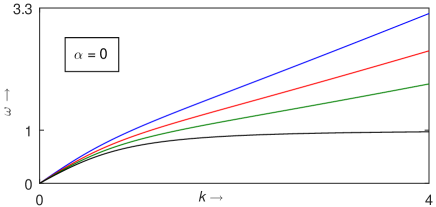
Figure 1: The normalized wave frequency ($\omega$) is plotted against the normalized wave number ($k$) for different values of number densities of ions by considering weakly coupled limit ($R\to 0$) of the dusty plasma. Here, blue curve corresponds to $\overline{N}_{i0}=1.1081$ and $\sigma_{d}=0.58$, red curve corresponds to $\overline{N}_{i0}=4.0540$ and $\sigma_{d}=0.33$, green curve corresponds to $\overline{N}_{i0}=6.7567$ and $\sigma_{d}=0.16$, and black curve corresponds to $\overline{N}_{i0}=6.7567$ and $\sigma_{d}=0$. The other values of the parameters are $\overline{N}_{e0}=\overline{N}_{i0}-1$, $\sigma_{ie}=0.01$ and $\gamma=1$.

Figure 2: The normalized wave frequency ($\omega$) is plotted against the normalized wave number ($k$) for all set of values of table 1 by considering the strongly coupled limit ($\alpha\neq 0$) of dusty plasma within the QLCA framework. Here, red dashed, blue dash-dotted and green solid curves correspond to the values of Set A, Set B and Set C respectively. The black dotted curve plotted when $\alpha=0$, i.e., when the dusty plasma system is weakly coupled.

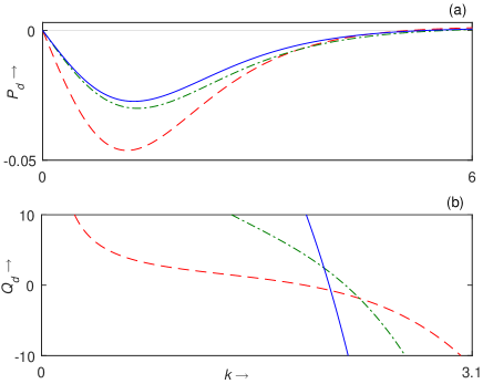
Figure 3: $P_{d}$ and $Q_{d}$ are plotted against $k$ in (a) and (b) respectively for weakly coupled limit of the dusty plasma, i.e., $R\to 0$. Here, the red dashed curve correspond to parametric values $h_{1}=1.1092$, $h_{2}=-0.5540$, $h_{3}=0.1847$, $\kappa=2.59$, $\sigma_{d}=0.58$, green curve dash dotted curve correspond to parametric values $h_{1}=2.9800$, $h_{2}=-1.4702$, $h_{3}=0.4902$, $\kappa=2.92$, $\sigma_{d}=0.57$, and blue solid curve correspond to parametric values $h_{1}=1.9308$, $h_{2}=-0.9615$, $h_{3}=0.3205$, $\kappa=2.99$, $\sigma_{d}=0.57$.

The dispersive coefficient ($P_{d}$) and nonlinear coefficient ($Q_{d}$) are plotted against $k$, for the weakly coupled limit ($D_{L}$ = 0) of dusty plasma, in figure 3, with three set of parameter given in table 1. The same qualitative nature of $P_{d}$ and $Q_{d}$ was also reported in strongly coupled limit of dusty plasma Sultana (2020).

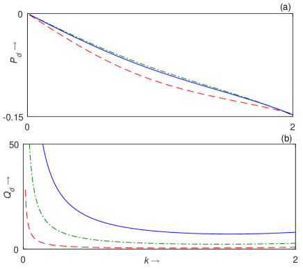
Figure 4: $P_{d}$ and $Q_{d}$ are plotted against $k$ in (a) and (b) respectively for strongly coupled limit of the dusty plasma within the QLCA framework. Here, the red dash dotted curve correspond to parametric values $h_{1}=1.1092$, $h_{2}=-0.5540$, $h_{3}=0.1847$, $\kappa=2.59$, $R=1.259$, $\sigma_{d}=0.00027$, green dashed curve correspond to parametric values $h_{1}=2.9800$, $h_{2}=-1.4702$, $h_{3}=0.4902$, $\kappa=2.92$, $R=1.292$, $\sigma_{d}=0.000353$ and blue solid curve correspond to parametric values $h_{1}=1.9308$, $h_{2}=-0.9615$, $h_{3}=0.3205$, $\kappa=2.99$, $R=1.299$, $\sigma_{d}=0.000462$.

From Fig. 3 and 4, we compare the weak and strong coupling effects on the coefficients $P_{d}$ and $Q_{d}$, as their product ($P_{d}Q_{d}$) decide the stable and unstable region. The red dashed, green dash dotted and blue solid line representing the coefficient $P_{d}$ and $Q_{d}$ for parameter $\kappa$ = 2.59, 2.92 and 2.99, respectively, with small value of $\sigma_{d}$. In both weak and strong coupling limit, the dispersive coefficient $P_{d}$ always remain negative, whereas in the weak coupling limit the nonlinear coefficient $Q_{d}$ has both negative as well as positive values depending upon the value of $\kappa$, and in the strongly coupled system it always remains positive at relatively high value of $\kappa$. In order to explore the lower $\kappa$ effects on the coefficients $P_{d}$ and $Q_{d}$ in the strong coupling limit, we have plotted the $P_{d}$ and $Q_{d}$ against $k$ with different small values of $\kappa$ in figure 5. It has also been identified, from Fig. 4, a negative threshold values of coefficient $Q_{d}$ arising at different value of wave-vector $k$. This negative threshold value appeared at relatively higher $k$ by increasing the value of $\kappa$ and, after $\kappa$ = 0.1825 coefficient $Q_{d}$ again attains positive value which remains positive for all value of $k$. The product $P_{d}Q_{d}$ against $k$ has been plotted in Fig. 6 with different small $\kappa$ values. It has been identified from Fig. 6 that the unstable region ($P_{d}Q_{d}$ $>$ 0), as presented with red and black curves, increases with an increment of $\kappa$ from 0.08 to 0.1. The threshold has been reached at $\kappa$ = 0.1825, as represented by blue line, after that modulated wave is stable ($P_{d}Q_{d}$ $<$ 0) for all $k$ and $\kappa$.

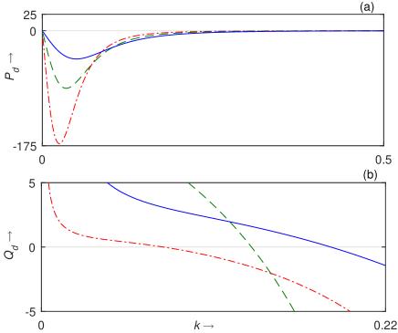
Figure 5: $P_{d}$ and $Q_{d}$ are plotted against $k$ in (a) and (b) respectively for strongly coupled limit of the dusty plasma within QLCA framework. Here, the red dash dotted curve correspond to parametric values $h_{1}=1.1092$, $h_{2}=-0.5540$, $h_{3}=0.1847$, $\kappa=0.05$, $R=1.005$, $\sigma_{d}=0.00027$, green dashed curve correspond to parametric values $h_{1}=2.9800$, $h_{2}=-1.4702$, $h_{3}=0.4902$, $\kappa=0.07$, $R=1.007$, $\sigma_{d}=0.000353$, and blue solid curve correspond to parametric values $h_{1}=1.9308$, $h_{2}=-0.9615$, $h_{3}=0.3205$, $\kappa=0.1$, $R=1.01$, $\sigma_{d}=0.000462$.

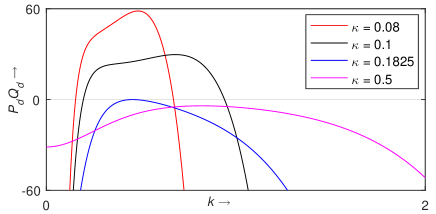
Figure 6: For strongly coupled limit of dusty plasma, the product of the coefficients of the nonlinear and dispersive term ($P_{d}Q_{d}$) is plotted against $k$ for different values of the screening parameter $\kappa$ and for $h_{1}=2.9800$, $h_{2}=-1.4702$, $h_{3}=0.4902$ $\sigma_{d}=0.000353$.

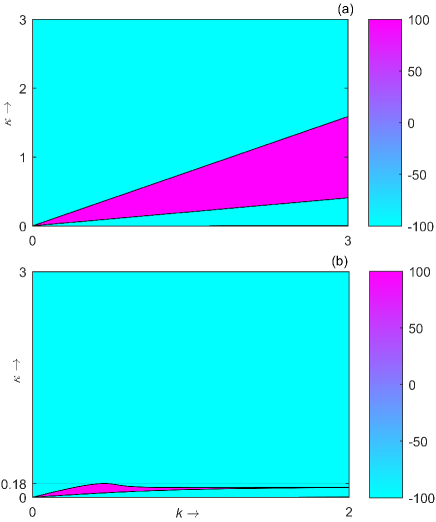
Figure 7: In Fig. 7(a) and 7(b), the contour of the product of the coefficients of dispersive and nonlinear terms, i.e., $P_{d}Q_{d}$ is represented here with respect to the wave number $k$ against the screening parameter $\kappa$ for the effect of weakly and strongly coupled dusty plasma respectively. For, $h_{1}=2.9800$, $h_{2}=-1.4702$, $h_{3}=0.4902$, $\sigma_{d}=0.000353$ and $\gamma=1$.

In order to compare the stable and unstable regions, in more detail, for weakly and strongly coupled limit, the contour plot of the product $P_{d}Q_{d}$ on $k-\kappa$ plane has been plotted in Fig. 7. It has been observed that a relatively larger unstable region (pink region) in weakly coupled limit, whereas in strongly coupled limit this unstable region is suppressed to a very small portion. In comparison to analysis of modulational instability in a one dimensional chain Amin et al. (1998c), where they have predicted an unstable region Amin et al. (1998c) for wide range of $\kappa$ value, our QLCA based analysis, which incorporates isotropy (3D structure) and explicit localization of constituent particles, has found completely stable region (cyan color) arising beyond $\kappa$ = 0.183 [see Fig 7(b) and Fig. 6]. It can be seen from Fig. 7(b) that the modulated wave become stable above threshold value $\kappa$ = 0.183 for all $k$.

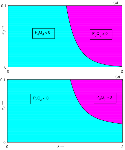
Figure 8: In Fig. 8(a) and 8(b), the contour of the product of the coefficients of dispersive and nonlinear terms, i.e., $P_{d}Q_{d}$ is represented here with respect to the wave number $k$ against $\sigma_{d}$ for weakly and strongly coupled dusty plasma respectively. Here, $h_{1}=2.9800$, $h_{2}=-1.4702$, $h_{3}=0.4902$, $\kappa=1.1$, $R=1.11$ and $\gamma=1$.

The effect of dust temperature via parameter $\sigma_{d}$ on the modulated wave has been presented in Fig 8, for both weak and strong coupling limit. For strong coupling limit, the contour plot of $P_{d}Q_{d}$ in $k-\sigma_{d}$ space shows that temperature enhances the unstable region (not presented in Fig. 7(b)). It can be seen in Fig. 8 that unstable region, represented by pink color region ($P_{d}Q_{d}$ $>$ 0), appears at relatively higher $k$ and $\sigma_{d}$ values. It can be concluded from these observations that temperature competes with the QLCA effects and at higher temperatures, the thermal effects dominate over the QLCA effects. The same trend has also been observed for weakly coupled limit of the present system.

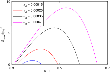
Figure 9: $G_{max}/|\phi_{0}|^{2}$ is plotted against $k$ for different values of $\sigma_{d}$ and for $h_{1}=2.9800$, $h_{2}=-1.4702$, $h_{3}=0.4902$, $\kappa=0.15$, $R=1.015$ and $\gamma=1$.

For strongly coupled limit, the maximum modulational growth rate of instability ($G_{max}/|\phi_{0}|^{2}$) is plotted against $k$ in Fig. 9 for different value of dust temperatures via $\sigma_{d}$ within the QLCA framework. The blue, red, black and pink color curves correspond to $\sigma_{d}=0.00015$, $\sigma_{d}=0.00025$, $\sigma_{d}=0.00035$ and $\sigma_{d}=0.0004$, respectively. It has been shown that the region of existence of the maximum modulational growth rate of instability increases with increasing $\sigma_{d}$. We can conclude that the dust temperature enhances the instability in the Yukawa system this trend is also predicted from the figure 8(b).

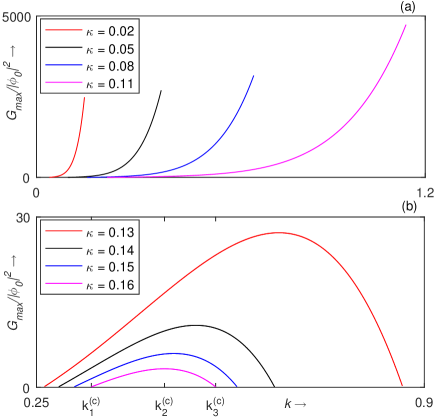
Figure 10: $G_{max}/|\phi_{0}|^{2}$ is plotted against $k$ for different values of $\kappa$ and for $h_{1}=2.9800$, $h_{2}=-1.4702$, $h_{3}=0.4902$, $\sigma_{d}=0.000353$ and $\gamma=1$.

For strongly coupled limit, $G_{max}/|\phi_{0}|^{2}$ is plotted against $k$ for different values of $\kappa$ in Fig 10. It can be seen that from Fig.10(a), that the MMGRI is increasing with $\kappa$ for 0.02 $\leq\kappa\leq$ 0.11. The MMGRI has been plotted with relatively higher values of $\kappa$ in Fig. 10(b), which shows that for fixed value of $\kappa$, the MMGRI first increase and after attaining a maximum value it again decreases until hit to the zero value. The peak value of MMGRI is reducing with $\kappa$ for 0.13 $\leq\kappa\leq$ 0.16 and as we already predicted that the MMGRI becomes zero at $\kappa$ = 0.183. It can be concluded that the modulated wave will become stable after $\kappa$ = 0.183 for all values of $k$. For example, we see that there exist the critical values $k_{1}^{(c)}=0.34201$, $k_{2}^{(c)}=0.46458$ and $k_{3}^{(c)}=0.55026$ of $k$ such that the MMGRI increases with increasing wave number ($k$) for $k_{1}^{(c)}<k<k_{2}^{(c)}$ and the MMGRI decreases with increasing wave number ($k$) for $k_{2}^{(c)}<k<k_{3}^{(c)}$ in figure 10(b). Finally, we can conclude that there exist the critical value $\kappa_{1}^{(c)}=0.1284$ and $\kappa_{2}^{(c)}=0.1821$ of $\kappa$ such that the MMGRI exists for $0<\kappa<\kappa_{2}^{(c)}$ and the MMGRI does not exists for $\kappa_{2}^{(c)}<\kappa<3$ because for these values of $\kappa$ the modulated wave became stable. This fact also confirms from Fig. 7(b).

Before concluding the discussion, a relevance can be drawn between dusty plasma excitation treated here and, for example, with the observation in RF field trapping of the ultracold ions Zhou and Ouyang (2021) where motion of signaling ion species was found to be tunable at the edge of the stability region as a result of ions being quasi-localized. The conclusion that collective ion interaction remains responsible for the observed delocalization in the boundary zone does indicate the role of constructively interacting collective ion excitation. The role of temperature of trapped species in this case can indeed be expected to be marginal as for Mathieu parameter $q\sim 1$, the mechanical motion of ions is entirely attributed to the collective (resonant) effect.

VI Conclusions

In this article, the QLCA based model has been adopted to study the MI of the DA waves in a strongly coupled Yukawa system consisting of negatively charged dust grains embedded in a polarizable plasma medium following the Boltzmann distribution. In order to study the modulated wave, we have derived the NLSE (39) using RPM Taniuti and Yajima (1969); Asano et al. (1969). It has been seen from the linear analysis that the DA wave frequency is reduced when the strong coupling effects are incorporated via QLCA framework Rosenberg and Kalman (1997). For the weak coupling case, it has been observed that the qualitative behaviour of the linear dispersion relation matches with the strongly coupled limit ($T^{\rm eff}$ model) Sultana (2020) in the dusty plasma. The MI of DA waves is numerically investigated for both the cases viz., for weakly and strongly coupled limits of the dusty plasma. It has been observed that in weakly coupled limit a relatively larger unstable region is recovered, whereas in strongly coupled limit this region is reduced to a very small zone of the parameter space. In comparison to analysis of modulation instability in a one-dimensional chain Amin et al. (1998c), where existing studies have predicted an unstable region Amin et al. (1998c) for wide range of $\kappa$ value, our QLCA based analysis incorporating explicit and isotropic localization of constituent particles, has recovered unstable region upto a relatively smaller value of $\kappa$ = 0.183 for a typical (small) dust temperature value $T_{d}\sim 10^{-4}Z_{d}T_{i}$. For strong coupling limit, the contour plot of $P_{d}Q_{d}$ in $k-\sigma_{d}$ space shows that the larger dust temperature enhances the unstable region dimension in the parameter space. The peak value of MMGRI is reducing with $\kappa$ for 0.13 $\leq\kappa\leq$ 0.16 and that MMGRI become zero at $\kappa$ = 0.183. The analysis on the instability criteria of a modulated wave, presented here, is largely applicable to quasi-crystalline state (amorphous solid) in which both free motion as well as localization of the constituent particles coexist. The presented results are therefore expected to cover a wide range of natural systems where modulational instability is the prime mechanism for the weakly nonlinear collective effects. As a relevant example, the case of collective interaction driven delocalization of RF trapped ultracold ions is discussed which is observed at the stability boundary in a recent experiment where the background interference of the RF trapping field drops sharply, leaving the trapped ion species to be in a quasi-localized state. Within the QLCA framework, the nonlinear excitations of MI of DA waves in strongly coupled dusty plasma can be a treated in presence of a magnetic field as a future study. The investigation on existence of envelope solitary waves, analytically as well as numerically, in a strongly coupled Yukawa system within QLCA framework can be another area to be explored.

References

- Koester and Schönberner (1986) D. Koester and D. Schönberner, Astron. Astrophys. 154, 125 (1986).
- Kouveliotou et al. (2001) C. Kouveliotou, J. E. Ventura, E. P. van den Heuvel, and E. P. J. van den Heuvel, The Neutron Star: Black Hole Connection, Vol. 567 (Springer Science & Business Media, 2001).
- Chabrier et al. (2002) G. Chabrier, F. Douchin, and A. Y. Potekhin, J. Phys.: Condens. Matter 14, 9133 (2002).
- Shukla et al. (1996) P. K. Shukla, S. V. Vladimirov, and M. Nambu, Phys. Scr. 53, 89 (1996).
- Rosenberg and Shukla (2011) M. Rosenberg and P. K. Shukla, Phys. Scr. 83, 015503 (2011).
- Golden et al. (1992) K. I. Golden, G. Kalman, and P. Wyns, Phys. Rev. A 46, 3463 (1992).
- Kalman et al. (1999) G. Kalman, V. Valtchinov, and K. I. Golden, Phys. Rev. Lett. 82, 3124 (1999).
- Rosenberg and Kalman (1998) M. Rosenberg and G. Kalman, AIP Conference Proceedings 446, 135 (1998).
- Merlino et al. (1998) R. L. Merlino, A. Barkan, C. Thompson, and N. D’angelo, Phys. Plasmas 5, 1607 (1998).
- Fortov et al. (2005) V. E. Fortov, A. V. Ivlev, S. A. Khrapak, A. G. Khrapak, and G. E. Morfill, Phys. Rep. 421, 1 (2005).
- Shukla and Mamun (2015) P. K. Shukla and A. A. Mamun, Introduction to dusty plasma physics (CRC press, 2015).
- Horanyi and Mendis (1985) M. Horanyi and D. A. Mendis, Astrophys. J. 294, 357 (1985).
- Horanyi and Mendis (1986) M. Horanyi and D. A. Mendis, The Astrophysical Journal 307, 800 (1986).
- Goertz (1989) C. K. Goertz, Rev. Geophys. 27, 271 (1989).
- Northrop (1992) T. G. Northrop, Phys. Scr. 45, 475 (1992).
- Tsytovich (1997) V. N. Tsytovich, Phys. Uspekhi 40, 53 (1997).
- Whipple (1981) E. C. Whipple, Rep. Prog. Phys. 44, 1197 (1981).
- Robinson and Coakley (1992) P. A. Robinson and P. Coakley, IEEE Trans. Electr. Insul. 27, 944 (1992).
- Rosenberg and Kalman (1997) M. Rosenberg and G. Kalman, Phys. Rev. E 56, 7166 (1997).
- Xie and Yu (2000) B. S. Xie and M. Y. Yu, Phys. Rev. E 62, 8501 (2000).
- Anowar et al. (2009) M. G. M. Anowar, M. S. Rahman, and A. A. Mamun, Phys. Plasmas 16, 053704 (2009).
- Yaroshenko et al. (2010) V. V. Yaroshenko, V. Nosenko, M. A. Hellberg, F. Verheest, H. M. Thomas, and G. E. Morfill, New J. Phys. 12, 073038 (2010).
- Wang et al. (2016) Y. L. Wang, X. Y. Guo, and Q. S. Li, Commun. Theor. Phys. 65, 247 (2016).
- Quinn and Goree (2000) R. A. Quinn and J. Goree, Phys. Plasmas 7, 3904 (2000).
- Amin et al. (1998a) M. R. Amin, G. E. Morfill, and P. K. Shukla, Phys. Rev. E 58, 6517 (1998a).
- Kourakis and Shukla (2003) I. Kourakis and P. K. Shukla, Phys. Plasmas 10, 3459 (2003).
- Kourakis and Shukla (2004) I. Kourakis and P. K. Shukla, Phys. Scr. 69, 316 (2004).
- Duan et al. (2004) W. s. Duan, J. Parkes, and L. Zhang, Phys. Plasmas 11, 3762 (2004).
- Misra and Chowdhury (2006) A. P. Misra and A. R. Chowdhury, Eur. Phys. J. D 39, 49 (2006).
- El-Taibany and Kourakis (2006) W. F. El-Taibany and I. Kourakis, Phys. plasmas 13, 062302 (2006).
- Gill et al. (2010) T. S. Gill, A. S. Bains, and C. Bedi, Phys. Plasmas 17, 013701 (2010).
- Bains et al. (2013) A. S. Bains, M. Tribeche, and C. S. Ng, Astrophys. Space Sci. 343, 621 (2013).
- Khaled et al. (2021) M. A. H. Khaled, M. A. Shukri, and A. A. Al-Shaibani, Braz. J. Phys. 51, 1290 (2021).
- Amin et al. (1998b) M. R. Amin, G. E. Morfill, and P. K. Shukla, Phys. Plasmas 5, 2578 (1998b).
- Amin et al. (1998c) M. R. Amin, G. E. Morfill, and P. K. Shukla, Phys. Scr. 58, 628 (1998c).
- Kourakis and Shukla (2006) I. Kourakis and P. K. Shukla, Int. J. Bifurcation Chaos 16, 1711 (2006).
- Sultana (2020) S. Sultana, Eur. Phys. J. D 74, 1 (2020).
- Ikezi (1986) H. Ikezi, Phys. Fluids 29, 1764 (1986).
- Thomas et al. (1994) H. Thomas, G. E. Morfill, V. Demmel, J. Goree, B. Feuerbacher, and D. Möhlmann, Phys. Rev. Lett. 73, 652 (1994).
- Chu and Lin (1994) J. H. Chu and I. Lin, Phys. Rev lett. 72, 4009 (1994).
- Misawa et al. (2001) T. Misawa, N. Ohno, K. Asano, M. Sawai, S. Takamura, and P. K. Kaw, Phys. Rev. Lett. 86, 1219 (2001).
- Xie et al. (2002) B. S. Xie, M. Y. Yu, K. F. He, Z. Y. Chen, and S. B. Liu, Phys. Rev. E 65, 027401 (2002).
- Chaudhuri et al. (2019) S. Chaudhuri, K. R. Chowdhury, and A. R. Chowdhury, Pramana 92, 1 (2019).
- El-Labany et al. (2015) S. K. El-Labany, E. F. El-Shamy, W. F. El Taibany, and N. A. Zedan, Chin. Phys. B 24, 035201 (2015).
- Kalman and Rosenberg (2003) G. J. Kalman and M. Rosenberg, J. Phys. A: Math. Gen. 36, 5963 (2003).
- Rosenberg et al. (2012) M. Rosenberg, G. J. Kalman, and P. Hartmann, Contr. Plasma Phys. 52, 70 (2012).
- Rosenberg et al. (2014) M. Rosenberg, G. J. Kalman, P. Hartmann, and J. Goree, Phys. Rev. E 89, 013103 (2014).
- Zhou and Ouyang (2021) X. Zhou and Z. Ouyang, Anal. Chem. 93, 5998 (2021).
- Chamel et al. (2016) N. Chamel, D. Page, and S. Reddy, in J. Phys.: Conf. Ser., Vol. 665 (IOP Publishing, 2016) p. 012065.
- Stacey (2007) W. M. Stacey, Fusion science and technology 52, 29 (2007).
- Killian et al. (2007) T. C. Killian, T. Pattard, T. Pohl, and J. Rost, Phys. Rep. 449, 77 (2007).
- Lyon and Rolston (2016) M. Lyon and S. Rolston, Rep. Prog. Phys. 80, 017001 (2016).
- Taniuti and Yajima (1969) T. Taniuti and N. Yajima, J. Math. Phys. 10, 1369 (1969).
- Asano et al. (1969) N. Asano, T. Taniuti, and N. Yajima, J. Math. Phys. 10, 2020 (1969).
- Kumar and Sharma (2021) P. Kumar and D. Sharma, Phys. Plasmas 28, 083704 (2021).
- Golden and Kalman (2000) K. I. Golden and G. J. Kalman, Phys.Plasmas 7, 14 (2000).
- Hou et al. (2004) L. J. Hou, Y. N. Wang, and Z. L. Mišković, Phys. Rev. E 70, 056406 (2004).
- Hou et al. (2009) L. J. Hou, Z. L. Mišković, A. Piel, and M. S. Murillo, Phys. Rev. E 79, 046412 (2009).
- Lado (1978) F. Lado, Phys. Rev. B 17, 2827 (1978).
- Hartmann et al. (2005) P. Hartmann, G. Kalman, Z. Donkó, and K. Kutasi, Phys. Rev. E 72, 026409 (2005).
- Khrapak et al. (2016) S. A. Khrapak, B. Klumov, L. Couedel, and H. M. Thomas, Phys. Plasmas 23, 023702 (2016).
- Dalui et al. (2017) S. Dalui, A. Bandyopadhyay, and K. P. Das, Phys. Plasmas 24, 042305 (2017).
- Khrapak (2017) S. A. Khrapak, AIP Advances 7, 125026 (2017).
- Fedele and Schamel (2002) R. Fedele and H. Schamel, Eur. Phys. J. B 27, 313 (2002).
- Fedele (2002) R. Fedele, Phys. Scr. 65, 502 (2002).
- Sikdar et al. (2018) A. Sikdar, A. Adak, S. Ghosh, and M. Khan, Phys. Plasmas 25, 052303 (2018).