Automatic Concept Extraction for Concept Bottleneck-based Video Classification

Abstract.

Recent efforts in interpretable deep learning models have shown that concept-based explanation methods achieve competitive accuracy with standard end-to-end models and enable reasoning and intervention about extracted high-level visual concepts from images, e.g., identifying the wing color and beak length for bird-species classification. However, these concept bottleneck models rely on a necessary and sufficient set of predefined concepts–which is intractable for complex tasks such as video classification. For complex tasks, the labels and the relationship between visual elements span many frames, e.g., identifying a bird flying or catching prey–necessitating concepts with various levels of abstraction. To this end, we present CoDEx, an automatic Concept Discovery and Extraction module that rigorously composes a necessary and sufficient set of concept abstractions for concept-based video classification. CoDEx identifies a rich set of complex concept abstractions from natural language explanations of videos–obviating the need to predefine the amorphous set of concepts. To demonstrate our method’s viability, we construct two new public datasets that combine existing complex video classification datasets with short, crowd-sourced natural language explanations for their labels. Our method elicits inherent complex concept abstractions in natural language to generalize concept-bottleneck methods to complex tasks.

1. Introduction

Deep neural networks (DNNs) provide unparalleled performance when applied to application domains, including video classification and activity recognition. However, the inherent black-box nature of the DNNs inhibits the ability to explain the output decisions of a model. While opaque decision-making may be sufficient for certain tasks, several critical and sensitive applications force model developers to face a dilemma between selecting the best-performing solution or one that is inherently explainable. For example, in the healthcare domain ((Yeung et al., 2019)), a life-or-death diagnosis compels the use of the best performing model, yet accepting an automated prediction without justification is wholly insufficient. Ideally, one could take advantage of the power of deep learning while still providing a sufficient understanding of why a model is making a particular decision, especially if the situation demands trust in a decision that can have severe impacts.

To address the need for model interpretability, researchers have sought to enable model intervention by leveraging concept bottleneck-based explanations. Unlike post hoc explanation methods–where techniques are used to extract an explanation for a given input for an inference by a trained black-box model ((Chakraborty et al., 2017; Jeyakumar et al., 2020)), concept bottleneck models are inherently interpretable and take a human reasoning-inspired approach to explaining a model inference based on an underlying set of concepts that define the decisions within an application. Thus far, prior works have focused on concept-based explanation models for image ((Kumar et al., 2009; Koh et al., 2020)) and text classification ((Murty et al., 2020)). However, the concepts are assumed to be given a priori by a domain expert–a process that may not result in a necessary and sufficient set of concepts. For instance, for bird species identification, an expert may have collected wing color but failed to collect beak color as a concept though it might be important for classification. More critically, prior works have considered simple concepts with the same level of abstraction, e.g., visual elements present in a single image. For more complex tasks such as video activity classification, a label may span multiple frames. Thus, the composing set of concepts will have various levels of abstraction representing relationships of various visual elements spanning multiple frames, e.g., a bird flapping its wings. So it is impractical to identify all the key concepts in advance. Therefore, unlike the prior works, we aim to exploit the complex abstractions inherent in natural language explanations to extract the set of important complex concepts.

Research Questions. In summary, this paper seeks to answer the following research questions:

• How can a machine automatically elicit the inherent complex concepts from natural language to construct a necessary and sufficient set of concepts for video classification tasks?

• Given that a machine can extract such concepts, are they informative and meaningful enough to be detected in videos by DNNs for downstream prediction tasks?

• Are the machine extracted concepts perceived by humans as good explanations for the correct classifications?

Approach. This paper introduces an automatic concept extraction module for concept bottleneck-based video classification. The bottleneck architecture equips a standard video classification model with an intermediate concept prediction layer that identifies concepts spanning multiple video frames. To compose the concepts that will be predicted by the model, we propose a natural language processing (NLP) based automatic Concept Discovery and Extraction module, CoDEx, to extract a rich set of concepts from natural language explanations of a video classification. NLP tools are leveraged to elicit inherent complex concept abstractions in natural language. CoDEx identifies and groups short textual fragments relating to events, thereby capturing the complex concepts from videos. Thus, we amortize the effort required to define and label the necessary and sufficient set of concepts. Moreover, we employ an attention mechanism to highlight and quantify which concepts are most important for a given decision.

To demonstrate the efficacy of our approach, we construct two new datasets–MLB V2E (Video to Explanations) for baseball activity classification and MSR-V2E for video category classification–that combine complex video classification datasets with short, crowd-sourced natural language explanations for their corresponding labels. We first compare our model against the existing standard end-to-end deep-learning methods for video classification and show that our architecture provides additional benefits of an inherently interpretable model with a marginal impact on performance (less than 0.3% accuracy loss on classification tasks). A subsequent user study showed that the extracted concepts were perceived by humans as good explanations for the classification on both the MLB-V2E and MSR-V2E datasets.

Contributions. We summarize our contributions as follows.

• We propose CoDEx, a concept discovery and extraction module that leverages NLP techniques to automatically extract complex concept abstractions from crowd-sourced, natural language explanations for a given video and label–obviating the need to manually pre-define a necessary and sufficient set of concepts thereby reducing the annotation effort.

• We construct two new public datasets, MLB-V2E and MSR-V2E, that combine complex video classification datasets with short, crowd-sourced natural language explanations and labels.

• We evaluate our approach on the two complex datasets and show that the concept-bottleneck model attains high concept accuracies while maintaining competitive task performance when compared to standard end-to-end video classification models.

• We also augment the concept-based explanation architecture to include an attention mechanism that highlights the importance of each concept for a given decision. We show that users prefer the concepts extracted by our method over baseline methods to explain a predicted label.

2. Related Work

There is a wide array of works in explainable deep learning for various applications. This work focuses on the concepts-based explanations for video classification, and this section provides an overview of the existing literature for overlapping domains.
Concept-Based Explanations for Images and Text. A number of existing works consider concept-bottleneck architectures where models are trained to interact with high-level concepts. Generally, the approaches are multi-task architectures, where the model first identifies a human-understandable set of concepts and then reasons about the identified concepts. Until now, the applications have been limited to static image and text applications. (Koh et al., 2020) used pre-labeled concepts provided by the dataset to train a model that predicts the concepts, which is then used to predict the final classification. However, the caveat is that the concepts had to be manually provided. (Ghorbani et al., 2019) and (Yeh et al., 2020) proposed approaches that automatically extract groups of pixels from the input image that represent meaningful concepts for the prediction. They were designed largely for image classification and extract concepts directly from the dataset. (Kim et al., 2018) propose a post-hoc explanation method that returns the importance of user-defined concepts for a classification. In the mentioned works, the concepts have been limited to simple concepts and are not suited for complex tasks such as video classification where we have complex concepts that may span multiple frames with various levels of abstraction.
Explanations for Video Classification Other approaches have been considered to explain video classification and activity recognition. (Chattopadhay et al., 2018) applied GradCAM and GradCAM++ to video classification, where for each frame, the important region of the frame to the model is highlighted as a heatmap. (Hiley et al., 2020) extract both spatial and temporal explanations from input videos by highlighting the relevant pixels. However, these are post-hoc techniques that focus on explaining black-box models, whereas our approach enables concept-bottleneck methods for video classification that are intended to be inherently interpretable and intervenable.
Video Captioning. In recent years, there is a large number of works ((Pan et al., 2017; Gao et al., 2017; Wang et al., 2018; Yan et al., 2019; Zhou et al., 2018; Chen and Jiang, 2021; Yu et al., 2017)) on video captioning. While they also employ natural language techniques, these works are tangential to generating text explanations for classifications, since they are merely describing the video. Our model provides an explanation justifying the classification of the video. Similarly, the associated datasets such as MSR-VTT ((Xu et al., 2016)) only have videos with ground truth captions that only describe the video without the context of a classification–which often results in concepts that do not pertain to a classification.
Semantic Concept Video Classification. The closest works to this paper is the body of work in semantic concept video classification ((Fan et al., 2004, 2007)), where the concepts are defined as salient objects that are visually distinguishable video components. The concepts in these works are simple objects detected in the videos and are not complex enough to capture the semantics of events that happen over multiple frames of the videos. These works typically used traditional SVM-based video classifiers.  (Assari et al., 2014) represent a video category based on the co-occurrences of the semantic concepts and classify based on the co-occurrences, but their method requires a predefined set of concepts. Thus, we now present the methodology behind our automatic concept extraction for concept bottleneck video classification.

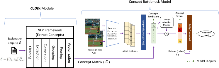
Figure 1. The overall pipeline showing the automatic concept extraction framework from natural language explanations and the concept bottleneck classification model training framework.

3. Concept Discovery and Bottleneck Video Classification

This work introduces CoDEx, an automatic concept extraction method from natural language explanations for concept-based video classification. Figure 1 depicts the overall concept-bottleneck pipeline, composed of CoDEx and the concept bottleneck model. CoDEx extracts a set of concepts from natural language explanations that will comprise the bottleneck layer for the video classification model. We first formalize the overall problem and then provide the methodology for both modules.

Problem Formalization. We assume that we have a training dataset $\{(x_{n},l_{n})\}_{n=1}^{N}=\mathcal{D}$ of videos $x_{n}$ with a label $l_{n}\in\mathcal{L}$, where $\mathcal{L}$ is a predefined set of possible class labels for the video. Each video is represented as a sequence of frames $f\in\mathcal{F}$ where $\mathcal{F}$ is the set of video frames. Thus video $x_{n}=\left<f_{n0},f_{n1},\ldots,f_{nT}\right>$ , where $f_{nt}$ represents frame $t$ of video $n$. For each video $x_{n}$, we form a label-explanation pair $(l_{n},e_{n})$, where $e_{n}$ is a (short) natural language document explaining the given label $l_{n}$. If multiple annotators contribute to an explanation for video-label pair, $(x_{n},l_{n})$ , then these are concatenated to form $e_{n}$. The full set of pairs $\mathcal{E}=\{(l_{n},e_{n})\}_{n=1}^{N}$ is the explanation corpus. Thus, the design goals are:

• Concept Discovery and Extraction (CoDEx) Module: Given the explanation corpus, first produce an $N\times K$ concept matrix, ${\bm{C}}$, where the $(n,k)$th element is $1$ if the $n$th explanation contains discovered concept $k$ and $0$ otherwise. We call the $n$th row $\bm{\mathbf{c}}_{n}$, the concept vector for video $x_{n}$. $K$ is the total number of discovered concepts.

• Concept Bottleneck Model: Given a concept matrix, ${\bm{C}}$, the second goal is to train a concept bottleneck model such that for a given video $x_{i}$, we predict a concept vector $\bm{\mathbf{c}}_{i}$–which indicates the presence or absence of concepts and their importance scores. The model then makes use of $\bm{\mathbf{c}}_{i}$ to make the final video classification.

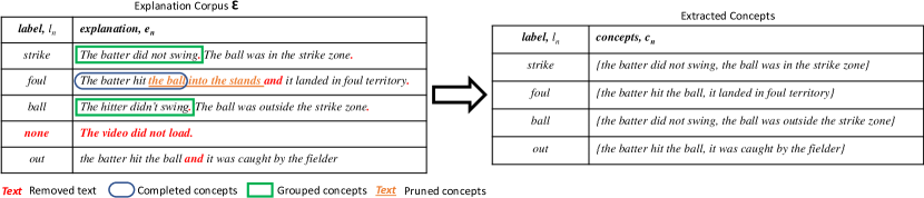
Figure 2. Running example for all six stages of the discovery pipeline module. The left table is the explanation corpus, with highlighted fragments to be modified. The right table contains the discovered concepts. The detailed step-by-step modifications are provided in Appendix A.1.

3.1. CoDEx: Concept Discovery and Extraction module

We now describe CoDEx, that extracts concepts from the explanation corpus, $\mathcal{E}$. The automatic extraction of the significant concepts is done in 6 steps, as outlined in Fig. 1. These are: cleaning, extraction, grouping, completion, pruning, and vectorization, which produce the final concept matrix, ${\bm{C}}$. Each of these steps are described below and illustrated with an example corpus depicted in Figure 2.

Cleaning. We remove explanations associated with corrupted or unlabeled videos from the explanation corpus. In Figure 2, this phase would remove the fourth row with the "none" label.

Extraction. The objective of this phase is to identify sentence constituents relevant to explaining the label. These text fragments, short sequences of words that appear in the document, are referred to as raw concepts. To achieve this, the cleaned explanation corpus is tokenized then passed through a pretrained constituency parser to recursively decompose the sentences. At each level of the constituency hierarchy, the text fragments are evaluated to determine whether they constitute a candidate raw concept. The rules for candidate raw concepts include the inclusion and exclusion rules mentioned in Table 1 and follow the widely adopted Universal POS tag naming convention for token types ((Petrov et al., 2012)). Every constituency parsed phrase that satisfies one of the two inclusion rules and not the exclusion rule is considered a candidate concept.

Rule Name	Rule
Inclusion 1	noun/pronoun → auxiliary (optional) → particle(optional)
Inclusion 2	noun/pronoun → auxiliary whose lemma is ‘be’ → any token
Exclusion	subordinating conjunction

Table 1. Inclusion and exclusion rules for candidate concepts.

After the extraction process is completed, we have a set of raw concepts, $\widetilde{\mathcal{K}}$, and each video is associated with a subset of these raw concepts. An example of extracted raw concepts, $\widetilde{\mathcal{K}}$, can be found in Appendix A.1.

Completion. There are instances where the pretrained constituency parser will split sentences midway through a text fragment in one sentence that was kept whole in another. For instance, in Figure 2, the constituency parser splits the explanation for "foul" such that "the batter hit the ball" is incorrectly excluded from the raw concepts. To ensure that those concepts are captured, we perform a substring lookup of each raw concept through all documents of the explanation corpus and count an explanation as containing a raw concept if it contains the corresponding raw concept as a substring. This does not change the number of raw concepts identified but increases their frequency counts.

Grouping (similar raw concepts). When identical text fragments are identified in different explanations, they are counted directly as the same raw concept. However, we would ideally like to treat superficially different concepts as the same if they essentially carry the same meaning, e.g., Figure 2 highlights two different raw concepts that carry the same meaning and hence can be grouped. For this, we use agglomerative clustering ((Müllner, 2011)) approach that measures the degree of difference between pairs of raw concepts and groups them together if they are similar enough. Our key contribution here is the distance metric used in clustering which is a novel measure of meta-distance between raw concepts. This measures the difference between concepts based on two aspects of the raw concepts: their linguistic difference and their difference in terms of the label categories with which they are associated.

We define meta-metric, $d$, as combining a linguistic distance, $d_{\text{text}}$ (capturing linguistic difference) as well as a meta-metric, $d_{\text{label}}$ (capturing the difference in the labels associated with each raw concept). More formally, for two raw concepts $\kappa_{i},\kappa_{j}\in\widetilde{\mathcal{K}}$ our distance is linear combination:

(1) $$d(\kappa_{i},\kappa_{j})=d_{\text{text}}(\bm{\mathbf{v}}_{i},\bm{\mathbf{v}}_{j})+\lambda d_{\text{label}}(\bm{\mathbf{n}}_{i},\bm{\mathbf{n}}_{j})$$

where $\bm{\mathbf{v}}_{i}$ is a sentence embedding for the text fragment of concept $\kappa_{i}$ (e.g., based on the BERT model (Devlin et al., 2019)), $d_{\text{text}}$ is a standard distance measure between vectors (e.g., cosine distance), $d_{\text{label}}$ is a meta-distance which aims to capture the similarity between two label count vectors, and $\lambda$ is a hyperparameter controlling the relative importance between textual and label distance. The inclusion of a label distance helps to distinguish between concepts that are superficially linguistically very simlar, but have very distinct meanings within the domain of interest. For instance, without the $d_{\text{label}}$, the concepts “the ball passed inside the strike zone” and “the ball passed outside the strike zone” will be grouped together though they are very different concepts as they have a very small $d_{\text{text}}$. We provide a more formal definition of the meta-metric $d_{\text{label}}$ more formally and provide some intuition behind its construction in Appendix A.2. We also exclude concept groups which occur rarely in the explanation corpus, with frequency less than some small threshold, $t$.

Pruning. Here, we seek a compact subset of concepts that, together, capture a high degree of information about the label while maintaining interpretability. More formally, after grouping, we have a set of raw concepts $\widetilde{\mathcal{K}}=\{\kappa_{1},\ldots,\kappa_{J}\}$, and we seek some subset of maximally informative concepts $\mathcal{K}^{\star}=\{\kappa_{j_{1}}\ldots,\kappa_{j_{K}}\}\subseteq\widetilde{\mathcal{K}}$.

To see what is meant by maximally informative, consider a randomly selected entry in the explanation corpus $(l,e)$. We define a binary random variable, ${\textnormal{C}}_{j}$ for each raw concept $\kappa_{j}$, and for any concept set $\mathcal{K}=\{\kappa_{j_{1}},\ldots,\kappa_{j_{K}}\}$, random vector $\bm{\mathbf{{\textnormal{C}}}}_{\mathcal{K}}=[{\textnormal{C}}_{1},\ldots,{\textnormal{C}}_{K}]$, such that ${\textnormal{C}}_{j}=1$ if $\kappa_{j}\in e$ and $0$ otherwise. $Y$ is the random variable which takes label $l$.

We wish to choose the smallest subset of concepts such that the mutual information (MI) between chosen concepts, $\mathcal{K}$, and label, $Y$, given by $I(Y;\bm{\mathbf{{\textnormal{C}}}}_{\mathcal{K}})$, is greater than a threshold fraction, $\gamma<1$ of the MI between the label and the complete concept vector, $I(Y;\bm{\mathbf{{\textnormal{C}}}}_{\widetilde{\mathcal{K}}})$. That is to say we wish to find $\mathcal{K}$ which satisfies:

(2) $$I(Y;\bm{\mathbf{{\textnormal{C}}}}_{\mathcal{K}}) \geq\gamma I(Y;\bm{\mathbf{{\textnormal{C}}}}_{\widetilde{\mathcal{K}}})$$

and where there is no subset $\mathcal{K}^{\prime}\subseteq\widetilde{\mathcal{K}}$ with $|\mathcal{K}^{\prime}|<|\mathcal{K}|$ which also satisfies Equation equation 2. In practice, this is infeasible as the problem is combinatorial. However, we note that $f(\mathcal{K})=I(Y;\bm{\mathbf{{\textnormal{C}}}}_{\mathcal{K}})$ is a monotone submodular set function of $\widetilde{\mathcal{K}}$. Given this, if we recursively construct a set of size $K$, by greedily adding single concepts that most improve the MI, the resulting set will be at least $1-\frac{1}{e}$ as good as the most informative set of size $K$ ((Nemhauser et al., 1978)). Therefore, we guarantee a highly-informative set $\mathcal{K}^{\star}$ by iteratively adding concepts to those previously selected, greedy with respect to the MI, until we have a set that satisfies Equation 2.

Vectorization. Each concept $\kappa_{j_{k}}\in\mathcal{K}^{\star}$ is given a unique index $k\in\{1,\ldots,K\}$, and each data-point, $x_{n}$ is associated with a concept vector $\bm{\mathbf{c}}_{n}=(c_{n1},\ldots,c_{nK})$, where $c_{nk}=1$ if $\kappa_{j_{k}}\in e_{n}$ and $0$ otherwise, indicating the presence or absence of the $k$th concept in the $n$th explanation. The collection of all the concept vectors gives an $N\times K$ concept matrix, ${\bm{C}}$.

3.2. Concept Bottleneck Model

We use the videos, the extracted concepts from CoDEx, and the labels to train an interpretable concept-bottleneck model to predict the activity and the corresponding concepts. Figure 1 shows the overview of our bottleneck architecture. The activity label, the concepts, and the corresponding concept scores are the outputs of the interpretable model and are indicated by dotted arrows in Figure 1.

Our bottleneck model architecture is based on the standard end-to-end video classification models where we use convolutional neural network-based feature extractors pretrained on the Imagenet dataset (Deng et al., 2009) to extract the spatial features from the videos. The features are then passed through temporal layers that can capture features across multiple frames which in turn is bottle-necked to predict the concepts. Lastly, we deploy an additive attention module (Bahdanau et al., 2014) that gives the concept score $\alpha_{c}$ indicating the importance of every concept to the classification. The attention module also improves the interpretability of the bottleneck model by indicating the key concepts for classification and this is evaluated in section 5. More details regarding the model architecture and hyper-parameters are in the Appendix A.4

Model loss function. The entire bottleneck classification model is trained in an end-to-end manner. Since the concepts are represented as binary vectors, we use sigmoid activation on the concept bottleneck layer and binary categorical loss function as the concept loss. The final layer of the classifier has softmax activations and categorical cross-entropy as the classification loss function. Thus, the overall loss function of the model is the sum of concept loss and the classification loss. The hyperparameter $\beta$ controls the tradeoff between concept loss, $L_{C}$, versus classification loss, $L_{Y}$ as shown in equation 3.

(3) $$Loss(L)=\frac{1}{N}\sum_{n=1}^{N}\left(L_{Y_{n}}+\beta\times L_{C_{n}}\right)\quad\text{where}\quad\beta>0$$

$$\text{and}\quad L_{Y_{n}} =-\sum_{j=1}^{m}y_{j}\log f_{S}(s_{j})$$

$$\text{and}\quad L_{C_{n}} =\sum_{k=1}^{l}\left[-c_{k}^{i}\log(f_{\sigma}(s_{k}))-(1-c_{k}\log(1-f_{\sigma}(s_{k})))\right]$$

$$\text{and}\quad f_{\sigma}(s_{i}) =\frac{1}{1+e^{-s_{i}}}\quad\text{,}\quad f_{S}(s_{i})=\frac{e^{s_{i}}}{\sum_{j=1}^{m}e^{s_{j}}}$$

Testing phase. Given an input test video, the model provides us with the activity prediction (label of the video), a concept vector indicating the relevant concepts that induced this classification and the concept importance score for each concept. By retrieving the phrase representing the concepts present in the video, the result obtained is a human-understandable explanation of the classification.

4. Implementation

To demonstrate our automatic concept extraction method, we construct two new datasets - MLB-V2E (Video to Explanations) and MSR-V2E, which combines short video clips with crowd-sourced classification labels and corresponding natural language explanations. For both datasets, we obtained a video activity label and natural language explanations for that label by crowd-sourcing on Amazon Mechanical Turk and used unrestricted text explanations to extract concepts automatically. For IRB exemption and compensation information, please refer to the Ethics Statement.

MLB-V2E Dataset: We used a subset of the MLB-Youtube video activity classification dataset introduced by  (Piergiovanni and Ryoo, 2018)–which had segmented video clips containing the five primary activities in baseball: strike, ball, foul, out, in play. We preprocessed the dataset and extracted 2000 segmented video clips where each video was 12 seconds long, 224$\times$224 in resolution, and recorded at 30 fps. To ensure that the quality of explanations is good, we screened over 450 participants. Based on their baseball knowledge, 150 participants were qualified to provide the natural language text explanations for our video clips. We have included a sample of our screening survey, the primary survey, and the explanations collected in the supplementary materials.

MSR-V2E Dataset: For this dataset, we used 2020 video clips from the MSR VTT dataset introduced by (Xu et al., 2016). The MSR-VTT dataset has general videos from everyday life and descriptions of these videos associated with them. Each video clip is between 10-30 seconds long, and approximately 200 participants provided the labels and explanations to construct the MSR-V2E dataset. The videos are classified into ten categories: Automobiles, Cooking, Beauty and Fashion, News, Science and Technology, Eating, Playing Sports, Music, Animals, and Family.
Figure 3 shows the number of videos belonging to each category in the MLB-V2E and the MSR-V2E datasets. Since the MSR-V2E dataset is imbalanced, we do some weighted oversampling while training to ensure that the models learn to predict all the classes.

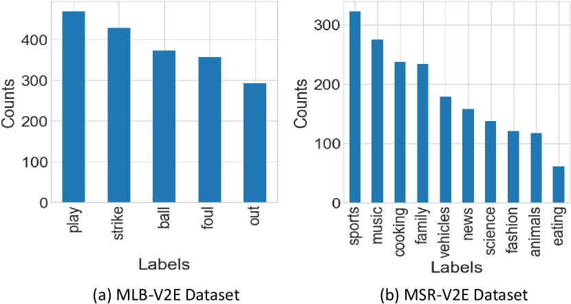
Figure 3. The number of videos belonging to each category on (a) the MLB-V2E dataset and (b) the MSR-V2E dataset

IRB Exemption and Compensation. This research study has been certified as exempt from review by the IRB and the participants were compensated at a rate of 15 USD per hour.

Dataset privacy. There was no personally identifiable information collected at anytime during the turk study. The responses provided by the mechanical turkers that are present in the dataset are completely anonymous.

Training: All our models were trained on 2 $\times$ Titan GTX GPUs using Adam optimizer. A summary of our entire model architecture and a trained model is provided in the supplementary materials.

5. Results

Number of extracted concepts. Table 2 shows that the system extracted 78 concepts and 62 concepts from the explanation corpus of MLB-V2E and MSR-V2E respectively.

Dataset	Number of Concepts after each Phase
	Extraction	Completion	Grouping	Pruning
MLB-V2E	1885	1885	225	78
MSR-V2E	1678	1678	104	62

Table 2. The number of concepts extracted by the Concept Discovery module from the explanation corpus after every phase.

The number of concepts remaining after the pruning phase is determined by the cumulative Mutual Information(MI) threshold. To identify the best threshold, we plotted the number of concepts at different thresholds versus performance of the model as shown in Figure 4.

We found that the task classification performance did not increase after a certain number of concepts and that optimal spot for the number of concepts corresponded to 90% Mutual Information.

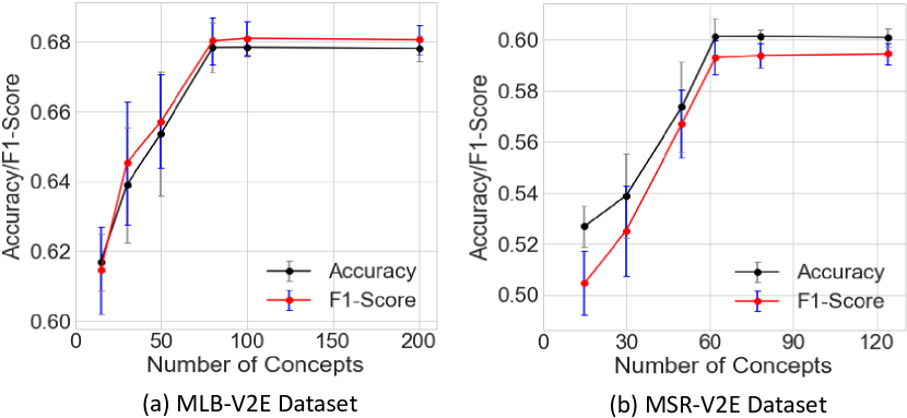
Figure 4. The number of concepts versus performance trade-off for the (a) the MLB-V2E dataset and (b) the MSR-V2E dataset.

Dataset	Model Type	Task Classification		Concepts
		Accuracy(%)	F1-score	AUC
MLB-V2E	Standard	68.42 $\pm$ 1.27	0.68 $\pm$ 0.011	-
	CB	68.16 $\pm$ 1.12	0.68 $\pm$ 0.004	0.85 $\pm$ 0.003
	CB + Attn.	68.38 $\pm$ 1.34	0.68 $\pm$ 0.004	0.88 $\pm$ 0.001
MSR-V2E	Standard	61.66 $\pm$ 1.42	0.60 $\pm$ 0.012	-
	CB	61.42 $\pm$ 1.18	0.60 $\pm$ 0.013	0.83 $\pm$ 0.006
	CB + Attn.	61.68 $\pm$ 1.23	0.60 $\pm$ 0.013	0.86 $\pm$ 0.004

Table 3. Performance of Models with Inception V3 as the feature extractor. ’CB’ refers to ’Concept Bottleneck’. The full table with results from different feature extractors can be found in Appendix A.5.

Comparing concept-bottleneck models to baselines. We adopt model architectures and hyperparameters from standard well -performing approaches that fall under 3 categories: 1) without concept bottleneck (Abdali and Al-Tuma, 2019), 2) with concept bottleneck (Koh et al., 2020), 3) with concept bottleneck and attention. We compared the performance of models with the bottleneck layer with standard video classification models without a concept bottleneck layer. We find that, though the latent space was constrained to the limited set of concepts extracted from the explanation corpus, bottleneck models performed as well as the unconstrained models, on both datasets. We also find that the addition of the attention layer improves the concept prediction of the models. Table 3 shows that concept bottleneck models achieved comparable task accuracy to standard black-box models on both tasks, despite the bottleneck constraint while achieving high concept prediction performance. All the models in the table used Inception-V3 as their feature extractor. Appendix A.5 shows the performance with other feature extractors.

Ablation Study of CoDEx. We performed an ablation study to highlight the impact of each stage in CoDEx’s pipeline. In the first experiment, we replaced the constituency parser-based extraction phase with word-level tokens obtained from the explanation corpus as concepts. We found that using word-level concepts significantly reduced both the task and the concepts prediction performance. We also evaluated how removing the grouping and pruning phases from the pipeline would impact performance. We observed that the grouping and pruning stages had a greater impact on the concept prediction performance that affected the explainability of the model. Table 4 shows the results of our study.

Dataset	Concepts Extraction	Task Acc (%)	Task F1-score	Concepts AUC
MLB-V2E	CoDEx	68.38	0.6802	0.8801
	w/o Extraction	63.47	0.5823	0.7285
	w/o Grouping	67.80	0.6772	0.7322
	w/o Pruning	68.36	0.6802	0.7719
	w/o Grouping & Pruning	65.29	0.6526	0.7021
MSR-V2E	CoDEx	61.68	0.6010	0.8600
	w/o Extraction	58.02	0.5214	0.7430
	w/o Grouping	59.31	0.5745	0.6888
	w/o Pruning	61.68	0.6010	0.7131
	w/o Grouping & Pruning	54.70	0.5178	0.6467

Table 4. Ablation Studies: Shows the effect of each step in CoDEx on model performance

Concept scores for interpretability. In addition to increasing the performance in concept prediction, the attention module also improves the explainability of the bottleneck model by providing an importance score for the concepts. Figure 5 shows the explanation from the concept bottleneck model with attention to test samples from the two datasets. The title shows the classification label, the y-axis indicates the top-3 concepts predicted as present in the video clip, and the x-axis corresponds to the concept score. $Others$ refers to the sum of the importance of all the remaining concepts.

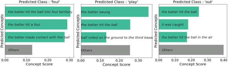
(a) MLB-V2E Dataset

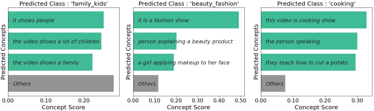
(b) MSR-V2E Dataset

Figure 5. Explanation offered by the model indicating the predicted class concepts present and their corresponding scores for (a) the MLB-V2E dataset (b) the MSR-V2E dataset.

Human study to evaluate concepts’ explainability. We performed a Mechanical Turk study to evaluate the explainability of our extracted complex concepts to the end-users. The participants were asked to select from four different options (presented in random) of what they consider to be the best possible Explanation for the classification of a given video. The four options are: Concepts predicted by bottleneck models without attention, Concepts predicted by bottleneck models with attention, Word-level concepts and a Random set of 2-5 concepts from the set of the most frequent concepts. The methodology of this study was inspired by (Chang et al., 2009)’s paper. Figure 6 presents the aggregated results of the Mechanical Turk study. The complex concepts predicted by the concept bottleneck model with attention was considered as the preferred explanation by 68% and 57% of the responses in the MLB-V2E and MSR-V2E datasets respectively followed by the concepts bottleneck models without attention in 20% and 28% of the responses for the two datasets. The presented confidence intervals are calculated using the bootstrap method as described by (DiCiccio and Efron, 1996) for 95% confidence.

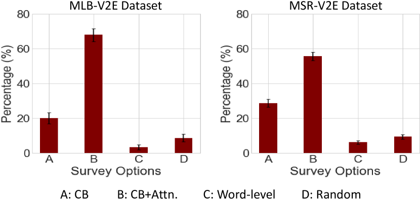
Figure 6. Survey responses with 95% bootstrap confidence interval for the two datasets. The participants preferred the concepts extracted by CoDEx and predicted by CB+Attn. as their preferred explanation by a significant margin.

Quantifying the Annotation effort. In prior works, annotating a dataset with concepts first requires identifying the necessary set of concepts that have to be annotated. Therefore, identifying the set of important concepts will either require a domain expert who has to provide a list of all the possible concepts or a separate study to identify the key concepts. Then annotating those concepts for each data point would require another study, making it more time-consuming and costly. Further, if the vocabulary of concepts is large, the annotation process would be inconvenient for the user. In our case, we significantly reduce the effort to identify and annotate the concepts with natural language explanations in a single user study. Moreover, natural language explanations can express richer compositions of concepts rather than simply identifying the presence or absence of an individual concept. To quantify the annotation effort, we conducted a small-scale study to annotate both MLB-V2E and MSR-V2E datasets with predefined concepts and compared it with the time it took to annotate with natural language explanations. For the MLB-V2E Dataset, we had a baseball domain expert who suggested thirty concepts to be annotated. For the MSR-V2E Dataset, we used the 62 concepts identified by CoDEx. The average time it took to complete per survey (each with ten videos) is indicated in Figure 7. We can see that the time it takes to annotate with text based explanations is 23.6% less for MLB-V2E Dataset and 30.8% less for MSR-V2E Dataset when compared to annotating with predefined concepts. We observe that the time to annotate increases with the increase in the number of concepts to be annotated.

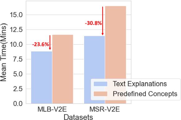
Figure 7. Average time taken to annotate 10 videos in a survey.

The helpfulness of extracted concepts in classification An MLP model trained on only the concepts (without video information) achieves a higher accuracy (7% for MLB-V2E and 4% for MSR-V2E) than the video classification model as shown in Table 5. This result indicates that the concepts extracted are meaningful for the classification task. Therefore, there is still headroom available if the concept bottleneck network can predict these initial concepts better from the videos.

Dataset	Task Accuracy(%)	Task F-1 score
MLB-V2E	75.68	0.7585
MSR-V2E	65.23	0.6422

Table 5. Performance of MLP classifier trained only on concepts (without videos)

The relationship between concepts and the classification task To understand the relationship between the extracted the concepts and the task classification, we compared the performance of the Concept Bottleneck models with a) MLP classifier b)Linear Classifier as the final classification layers. The results showed that there was approximately 2% drop in classification performance when using a Linear Classifier instead of an MLP as indicated in Table 6. This indicates that, the classification task is not just a simple linear combination of the extracted concepts and the composition of concepts is important for classification.

Dataset	Accuracy (%)		Difference (%)
	MLP	Linear Classifier
MLB-V2E	68.38	66.94	-1.44
MSR-V2E	61.68	60.02	-1.66

Table 6. Comparison of the performance of Bottleneck models with MLP classifier and Linear Classifier

6. Discussion

The Application of Concept-Bottleneck based models. This method of using Concept Bottleneck Models is only applicable to those tasks where an explanation by concepts is applicable. In other words, it is suitable for complex classification tasks where the predictions can be explained in terms of more atomic concepts. We see our method as valuable in human decision support with video surveillance or video retrieval from large datasets based on higher-level concepts. In those domains, it is the decomposition of higher-level events into more atomic events that is key.

Representative Concept. Our concept extraction method selects the most frequent concept in a grouped cluster as the representative concept. In general, the most frequent concept suffices to explain a particular component of the complex activity. However, there were some instances where the most frequent concept would have a specific terminology rather than a general term, e.g., "left fielder" is a subclass of "outfielder." Future work can strive towards generating the representative concept for a cluster, as opposed to opting for the most frequent or popular phrasing.
Generalizability and Tractability of Crowdsourced Concepts. Generalizing our method to other domains is tractable we do not require a domain expert to formalize the survey questions, i.e., one only needs to ask, "why does this video have this label?" Further, crowdsourcing enables a richer set of concepts rather than relying on one domain expert to provide the necessary and sufficient set of concepts.
Preserving Spatial-temporal Semantics. Our model’s output explanation currently provides a set of activated concepts along with their score. However, they do not capture the spatial and temporal relationships between concepts. Some rich concepts implicitly embed spatial and temporal properties, e.g., “the batter hit the ball on the ground" implies the following sequence: a batter swung at a ball, made contact with the ball, and the ball landed on the ground. However, if the generated set of concepts is limited to less informative concepts, e.g., “the batter," the spatial and temporal ordering of concepts matters. Future work can generalize the architecture to generate concept-based natural language explanations that explicitly preserve spatial-temporal semantics.
Neural-symbolic Reasoning. Our model’s reasoning layers are inherently black-box in nature, i.e., the concept vectors are fed into a fully connected network. To further bolster human-machine teaming and interpretability, the final classification model can be replaced with a rule-based model–analogous to prior works that fuse deep learning inferences with symbolic reasoning layers for complex event detection ((Xing et al., 2020; Vilamala et al., 2019)).

7. Conclusion

The remarkable performance of deep neural networks is only limited by the stark limitation in clearly explaining their inner workings. While researchers have introduced feature highlighting post-hoc explanation techniques to provide insight into these black-box models, the inherently interpretable concept-bottleneck models offer a promising new approach to explanation by decomposing application tasks into a set of underlying concepts. We build upon concept-based explanations by introducing an automatic concept extraction module, CoDEx, to a general concept bottleneck architecture for identifying, training, and explaining video classification tasks. In coalescing concept definitions across crowd-sourced explanations, CoDEx amortizes the hardship of manually pre-defining the concepts while reducing the burden on the data annotators. We also show that our method provides reasonable explanations for classification without compromising performance compared to standard end-to-end video classification models.

Appendix A Appendix

A.1. Running Example to describe the Concept Discovery and Extraction Pipeline

Example 0 (A simple Explanation corpus).

Consider using baseball domain with a few meaningful labels, a null label $\mathcal{L}=\{\text{strike},\text{ball},\text{foul},\text{out},\text{none}\}$ and five entries in the explanation corpus $\mathcal{E}$:

id, $n$	label, $l_{n}$	explanation, $e_{n}$
$1$	strike	The batter did not swing. The ball was in the strike zone.
$2$	foul	the batter hit the ball into the stands and it landed in foul territory
$3$	ball	The hitter didn’t swing. The ball was outside the strike zone.
$4$	none	The video did not load.
$5$	out	the batter hit the ball and it was caught by the fielder

Step 0 (After Cleaning Phase).

The none label entry is removed after the Cleaning phase

id, $n$	label, $l_{n}$	explanation, $e_{n}$
$1$	strike	The batter did not swing. The ball was in the strike zone.
$2$	foul	the batter hit the ball into the stands and it landed in foul territory.
$3$	ball	The hitter didn’t swing. The ball was outside the strike zone.
$4$	out	the batter hit the ball and it was caught by the fielder

Step 0 (After Extraction Phase).

The raw concepts are extracted based on the defined rules discussed in Table 1 corresponding to each explanation with the help of a pre-trained constituency parser.

id, $n$	label, $l_{n}$	raw concepts, $\widetilde{\mathcal{K}}$
$1$	strike	The batter did not swing, The ball was in the strike zone
$2$	foul	the ball into the stands, it landed in foul territory
$3$	ball	The hitter didn’t swing, The ball was outside the strike zone
$4$	out	the batter hit the ball, it was caught by the fielder

Step 0 (After Completion Phase).

The concept ’the batter hit the ball’ was not extracted by the Extraction phase for the Id $2$ explanation in this corpus. This missing concept is retrieved through the sub-string matching.

id, $n$	label, $l_{n}$	raw concepts, $\widetilde{\mathcal{K}}$
$1$	strike	The batter did not swing, The ball was in the strike zone
$2$	foul	the batter hit the ball, the ball into the stands, it landed in foul territory
$3$	ball	The hitter didn’t swing, The ball was outside the strike zone
$4$	out	the batter hit the ball, it was caught by the fielder

Step 0 (After Grouping Phase).

We show the grouped concepts for this example corpus

Concept-id, $i$	Concept groups
$1$	[The batter did not swing, The hitter didn’t swing]
$2$	[the batter hit the ball, the batter hit the ball]
$3$	[The ball was in the strike zone]
$4$	[The ball into the stands]
$5$	[it landed in foul territory]
$6$	[The ball was outside the strike zone]
$7$	[it was caught by the fielder]

Step 0 (After Pruning Phase).

The concept ’the ball into the stands’ of Concept-Index 4 from previous table was not contributing much and hence was pruned.

Concept-id, $i$	Concept groups
$1$	[The batter did not swing, The hitter didn’t swing]
$2$	[the batter hit the ball, the batter hit the ball]
$3$	[The ball was in the strike zone]
$4$	[it landed in foul territory]
$5$	[The ball was outside the strike zone]
$6$	[it was caught by the fielder]

Step 0 (After Vectorization).

After pruning, each sample is mapped to their corresponding concept vector. The value of concept vector at index $i$ is $1$ if $e_{n}$ has the concept with index $i$, else, it’s $0$. The Matrix containing all the concept vectors is called the Concept Matrix, ${\bm{C}}$

id, $n$	label, $l_{n}$	Concept Vector, $\bm{\mathbf{c}}_{n}$
$1$	strike	[1,0,1,0,0,0]
$2$	foul	[0,1,0,1,0,0]
$3$	ball	[1,0,0,0,1,0]
$4$	out	[0,1,0,0,0,1]

A.2. Meta-distance for label based proximity

At the end of the Completion Phase we define a count for each raw concept, $\kappa_{i}\in\widetilde{\mathcal{K}}$, given by $M_{i}$. And for each label category $l\in\mathcal{L}$, we define a label count for raw concept $\kappa_{i}$ as $m_{il}$ where $i$ is the index of the concept. These count the presence of raw concepts explanations, and $\sum_{l\in\mathcal{L}}m_{il}=M_{i}$. Finally we group together raw concept $\kappa_{i}$’s label counts into a label count vector $\bm{\mathbf{m}}_{i}=[m_{i1},\ldots,m_{i|\mathcal{L}|}]$

Now we describe the meta-metric $d_{\text{label}}$ used in the Grouping phase more formally and provide some intuition behind its construction. Consider that we have two raw concepts $\kappa_{i},\kappa_{j}\in\widetilde{\mathcal{K}}$ and label count vectors $\bm{\mathbf{m}}_{i}$ and $\bm{\mathbf{m}}_{j}$. We next assume that vector $\bm{\mathbf{m}}_{i}$ constitutes $M_{i}$ i.i.d. draws from a categorical distribution with unknown parameters $\bm{\mathbf{\mu}}_{i}=(\mu_{il})_{l=1}^{|\mathcal{L}|}$, where $\mu_{il}$ is the probability that a randomly selected occurrence of raw concept $i$ belongs to an entry in the explanation corpus with label category $l$. Our label distance $d_{\text{label}}$ is the evidence ratio between the count vectors, $\bm{\mathbf{m}}_{i}$ and $\bm{\mathbf{m}}_{j}$, being drawn from independent categorical distributions (model $\mathcal{M}_{\text{indp}}$) versus them being drawn from the same distribution (model $\mathcal{M}_{\text{comb}}$). More precisely,

$$d_{\text{label}}(\bm{\mathbf{m}}_{i},\bm{\mathbf{m}}_{j})=\frac{p(\bm{\mathbf{m}}_{i},\bm{\mathbf{m}}_{j}|\mathcal{M}_{\text{indp}})}{p(\bm{\mathbf{m}}_{i},\bm{\mathbf{m}}_{j}|\mathcal{M}_{\text{comb}})}$$

Note that this is not a true distance between count vectors as two identical count vectors do not have a distance of zero. Nonetheless, it satisfies the other requirements of a metric: non-negativity, symmetry and the triangle inequality, and two vectors that are more (less) likely to come from the same multinomial will have a distance less (more) than $1$.

To evaluate the label distance we must calculate the evidence for various categorical samples given the model $p(\bm{\mathbf{m}}|\bm{\mathbf{\mu}},M)$ . For simplicity, we assume total count $M$ is known and define a Dirichlet prior $p(\bm{\mathbf{\mu}}|\alpha\bm{\mathbf{1}})$ where $\bm{\mathbf{1}}$ is the vector of all $1$s (this makes the simplifying assumption that the prior is symmetric). The evidence for $\bm{\mathbf{m}}$ is then:

$$p(\bm{\mathbf{m}}|\alpha)=\int p(\bm{\mathbf{m}}|\bm{\mathbf{\mu}},M)p(\bm{\mathbf{\mu}}|\alpha\textbf{1})d\bm{\mu}$$

The label meta-metric is the evidence ratio given by:

$$d_{\text{label}}(\bm{\mathbf{m}}_{i},\bm{\mathbf{m}}_{j})=\frac{p(\bm{\mathbf{m}}_{i}|\alpha)p(\bm{\mathbf{m}}_{j}|\alpha)}{p(\bm{\mathbf{m}}_{i}+\bm{\mathbf{m}}_{j}|\alpha)}$$

For computational efficiency (and since it did not appear to affect results measurably) we use an approximation for $p(\bm{\mathbf{m}}|\alpha)$ in our calculation of $d_{l}$.

We first evaluate the expected parameter of the posterior distribution given count vector $\bm{\mathbf{m}}$, namely

$$\tilde{\bm{\mathbf{\mu}}}=\mathbb{E}[\bm{\mathbf{\mu}}|\alpha,\bm{\mathbf{m}}]$$

then evaluate the evidence for $\bm{\mathbf{m}}$ conditioned on $\tilde{\bm{\mathbf{\mu}}}$, i.e.

$$p(\bm{\mathbf{m}}|\tilde{\bm{\mathbf{\mu}}})=\prod_{k=1}^{K}\left(\frac{m_{il}+\alpha}{M_{i}+K\alpha}\right)^{m_{il}}$$

We then calculate $\log d_{\text{label}}(\bm{\mathbf{m}}_{i},\bm{\mathbf{m}}_{j})$ and exponentiate to improve precision. After grouping, the raw concept within a cluster with highest frequency is identified as the representative concept of that cluster.

A.3. Language Models

A.3.1. Concept Extraction

After obtaining the free form textual explanations for both datasets, we first cleaned them by removing explanations associated with corrupted video files and the videos which were labelled incorrectly. We then considered three different Spacy’s pretrained constituency parsers: $en\_core\_web\_lg$, $en\_core\_web\_md$, $en\_core\_web\_sm$ to parse the explanations and extract raw concepts based on the rules discussed in section 3.1. We found that, the parser $en\_core\_web\_lg$ was more accurate in identifying the constituents and resulted in better concept extraction.

A.3.2. Concept Grouping

For text distance we embedded the raw concepts with a sentence encoder and we experimented with two models: paraphrase-distilroberta-base-v1 (distil) (Sanh et al., 2019) and stsb -roberta-base (stsb) (Reimers and Gurevych, 2019) into a 768 dimensional space both using the sentence_transformer python library.

And to cluster the semantically similar concepts together using agglomerative clustering (Müllner, 2011), we evaluated a variety of distance metrics within the resulting 768-dimensional space, including: Our proposed meta-distance metric, Chebyshev (infinity norm), manhattan, Euclidean and cosine distances. To select hyperparameters, including prior $\alpha$ for label distance, and relative importance factor $\lambda$ we performed a grid search and selected the values that resulted in well-formed clusters. Based on our experiments (Provided in code), we found that stsb encoder with our proposed meta-distance metric resulted in the best grouping of concepts. Note: $d_{text}$ can be either cosine or manhattan distance as they gave similar clusters.

After clustering, we set the frequency occurrence threshold of $3$ and removed the rare concept groups which occurred less than this threshold. Then, pruning was done using 90% of mutual information score as discussed in section 3.1 which resulted in 78 significant concepts for our MLB-V2E dataset and 62 concepts for MSR-V2E dataset as shown in Table 2. Therefore, each video was associated with a binary concept vector of shape $[1\times k]$ where k is the number of concepts, indicating the presence and absence of each concept.

A.4. The Classification Models

We considered three different feature extractors : Resnet 50v2 (He et al., 2016), Resnet 101v2 (He et al., 2016) and InceptionV3 (Szegedy et al., 2016) models and pretrained on the Imagenet dataset to extract features from each frame of our video clips. We excluded the final classification layer from these models and did a global maxpool across the width and height such that we get a $2048$ size feature vector for every frame. We then concatenate the features together, resulting in a $[2048\times 360]$ feature matrix for every video where $360$ is the number of frames per video.

For the Temporal Layer, we considered both temporal convolution (Lea et al., 2017) and LSTM (Hochreiter and Schmidhuber, 1997) based architectures which are good at extracting temporal features and found that Temporal CNNs outperformed LSTM by a significant amount. And the Bottleneck Layer is a dense layer with $k$ neurons and hence the output is a vector of shape $[1\times k]$ where $k$ is the number of significant concepts. We introduced an attention layer in the concept-bottleneck model that gives the concept score for each concept. The final fully connected layer is implemented with $L$ neurons (L classes) which predicts the class from the video.

A.5. Performance of Models

Table 7 and Table 8 show the performance of all the models with different feature extractors on the two datasets. Each model was trained thrice and the mean and standard deviation of the performance are reported. We find that models with Inception V3 as the feature extractor performed the best. Adding attention mechanism improved the performance of concepts prediction and also achieved higher accuracies than the concept bottleneck models without attention.

Feature Extractor	Model Type	Task Classification		Concepts
		Accuracy(%)	F1-score	AUC
Resnet 50V2	Standard	67.92 $\pm$ 0.78	0.68 $\pm$ 0.003	-
	CB	67.83 $\pm$ 0.74	0.68 $\pm$ 0.001	0.85 $\pm$ 0.005
	CB + Attn.	67.96 $\pm$ 0.65	0.68 $\pm$ 0.002	0.88 $\pm$ 0.002
Resnet 101V2	Standard	68.18 $\pm$ 0.88	0.68 $\pm$ 0.005	-
	CB	68.01 $\pm$ 1.02	0.68 $\pm$ 0.013	0.85 $\pm$ 0.004
	CB + Attn.	68.26 $\pm$ 1.12	0.68 $\pm$ 0.009	0.88 $\pm$ 0.000
Inception V3	Standard	68.46 $\pm$ 1.27	0.68 $\pm$ 0.011	-
	CB	68.16 $\pm$ 1.12	0.68 $\pm$ 0.004	0.85 $\pm$ 0.003
	CB + Attn.	68.38 $\pm$ 1.34	0.68 $\pm$ 0.004	0.88 $\pm$ 0.001

Table 7. Performance of Models on the MLB-V2E Dataset

Feature Extractor	Model Type	Task Classification		Concepts
		Accuracy(%)	F1-score	AUC
Resnet 50V2	Standard	61.52 $\pm$ 1.20	0.59 $\pm$ 0.008	-
	CB	61.23 $\pm$ 1.71	0.59 $\pm$ 0.008	0.82 $\pm$ 0.009
	CB + Attn	61.28 $\pm$ 1.54	0.59 $\pm$ 0.007	0.86 $\pm$ 0.004
Resnet 101V2	Standard	61.56 $\pm$ 1.31	0.60 $\pm$ 0.008	-
	CB	61.38 $\pm$ 1.24	0.60 $\pm$ 0.008	0.83 $\pm$ 0.006
	CB + Attn.	61.44 $\pm$ 1.32	0.60 $\pm$ 0.009	0.86 $\pm$ 0.003
Inception V3	Standard	61.79 $\pm$ 1.42	0.60 $\pm$ 0.012	-
	CB	61.42 $\pm$ 1.18	0.60 $\pm$ 0.013	0.83 $\pm$ 0.006
	CB + Attn.	61.68 $\pm$ 1.23	0.60 $\pm$ 0.009	0.86 $\pm$ 0.004

Table 8. Performance of Models on the MSR-V2E Dataset

References

- (1)
- Abdali and Al-Tuma (2019) Al-Maamoon R Abdali and Rana F Al-Tuma. 2019. Robust real-time violence detection in video using cnn and lstm. In 2019 2nd Scientific Conference of Computer Sciences (SCCS). IEEE, 104–108.
- Assari et al. (2014) Shayan Modiri Assari, Amir Roshan Zamir, and Mubarak Shah. 2014. Video classification using semantic concept co-occurrences. In 2014 IEEE Conference on Computer Vision and Pattern Recognition. IEEE, 2529–2536.
- Bahdanau et al. (2014) Dzmitry Bahdanau, Kyunghyun Cho, and Yoshua Bengio. 2014. Neural machine translation by jointly learning to align and translate. arXiv preprint arXiv:1409.0473 (2014).
- Chakraborty et al. (2017) Supriyo Chakraborty, Richard Tomsett, Ramya Raghavendra, Daniel Harborne, Moustafa Alzantot, Federico Cerutti, Mani Srivastava, Alun Preece, Simon Julier, Raghuveer M Rao, et al. 2017. Interpretability of deep learning models: a survey of results. In 2017 IEEE smartworld, ubiquitous intelligence & computing, advanced & trusted computed, scalable computing & communications, cloud & big data computing, Internet of people and smart city innovation (smartworld/SCALCOM/UIC/ATC/CBDcom/IOP/SCI). IEEE, 1–6.
- Chang et al. (2009) Jonathan Chang, Sean Gerrish, Chong Wang, Jordan L Boyd-Graber, and David M Blei. 2009. Reading tea leaves: How humans interpret topic models. In Advances in neural information processing systems. 288–296.
- Chattopadhay et al. (2018) Aditya Chattopadhay, Anirban Sarkar, Prantik Howlader, and Vineeth N Balasubramanian. 2018. Grad-cam++: Generalized gradient-based visual explanations for deep convolutional networks. In 2018 IEEE Winter Conference on Applications of Computer Vision (WACV). IEEE, 839–847.
- Chen and Jiang (2021) Shaoxiang Chen and Yu-Gang Jiang. 2021. Towards Bridging Event Captioner and Sentence Localizer for Weakly Supervised Dense Event Captioning. In Proceedings of the IEEE/CVF Conference on Computer Vision and Pattern Recognition. 8425–8435.
- Deng et al. (2009) Jia Deng, Wei Dong, Richard Socher, Li-Jia Li, Kai Li, and Li Fei-Fei. 2009. Imagenet: A large-scale hierarchical image database. In 2009 IEEE conference on computer vision and pattern recognition. Ieee, 248–255.
- Devlin et al. (2019) Jacob Devlin, Ming-Wei Chang, Kenton Lee, and Kristina Toutanova. 2019. BERT: Pre-training of Deep Bidirectional Transformers for Language Understanding. arXiv:1810.04805 [cs.CL]
- DiCiccio and Efron (1996) Thomas J DiCiccio and Bradley Efron. 1996. Bootstrap confidence intervals. Statistical science 11, 3 (1996), 189–228.
- Fan et al. (2007) Jianping Fan, Hangzai Luo, Yuli Gao, and Ramesh Jain. 2007. Incorporating concept ontology for hierarchical video classification, annotation, and visualization. IEEE Transactions on Multimedia 9, 5 (2007), 939–957.
- Fan et al. (2004) Jianping Fan, Hangzai Luo, Jing Xiao, and Lide Wu. 2004. Semantic video classification and feature subset selection under context and concept uncertainty. In Proceedings of the 2004 Joint ACM/IEEE Conference on Digital Libraries, 2004. IEEE, 192–201.
- Gao et al. (2017) Lianli Gao, Zhao Guo, Hanwang Zhang, Xing Xu, and Heng Tao Shen. 2017. Video captioning with attention-based LSTM and semantic consistency. IEEE Transactions on Multimedia 19, 9 (2017), 2045–2055.
- Ghorbani et al. (2019) Amirata Ghorbani, James Wexler, James Zou, and Been Kim. 2019. Towards automatic concept-based explanations. arXiv preprint arXiv:1902.03129 (2019).
- He et al. (2016) Kaiming He, Xiangyu Zhang, Shaoqing Ren, and Jian Sun. 2016. Deep residual learning for image recognition. In Proceedings of the IEEE conference on computer vision and pattern recognition. 770–778.
- Hiley et al. (2020) Liam Hiley, Alun Preece, Yulia Hicks, Supriyo Chakraborty, Prudhvi Gurram, and Richard Tomsett. 2020. Explaining motion relevance for activity recognition in video deep learning models. arXiv preprint arXiv:2003.14285 (2020).
- Hochreiter and Schmidhuber (1997) Sepp Hochreiter and Jürgen Schmidhuber. 1997. Long short-term memory. Neural computation 9, 8 (1997), 1735–1780.
- Jeyakumar et al. (2020) Jeya Vikranth Jeyakumar, Joseph Noor, Yu-Hsi Cheng, Luis Garcia, and Mani Srivastava. 2020. How Can I Explain This to You? An Empirical Study of Deep Neural Network Explanation Methods. Advances in Neural Information Processing Systems 33 (2020).
- Kim et al. (2018) Been Kim, Martin Wattenberg, Justin Gilmer, Carrie Cai, James Wexler, Fernanda Viegas, et al. 2018. Interpretability beyond feature attribution: Quantitative testing with concept activation vectors (tcav). In International conference on machine learning. PMLR, 2668–2677.
- Koh et al. (2020) Pang Wei Koh, Thao Nguyen, Yew Siang Tang, Stephen Mussmann, Emma Pierson, Been Kim, and Percy Liang. 2020. Concept bottleneck models. In International Conference on Machine Learning. PMLR, 5338–5348.
- Kumar et al. (2009) Neeraj Kumar, Alexander C Berg, Peter N Belhumeur, and Shree K Nayar. 2009. Attribute and simile classifiers for face verification. In 2009 IEEE 12th international conference on computer vision. IEEE, 365–372.
- Lea et al. (2017) Colin Lea, Michael D Flynn, Rene Vidal, Austin Reiter, and Gregory D Hager. 2017. Temporal convolutional networks for action segmentation and detection. In proceedings of the IEEE Conference on Computer Vision and Pattern Recognition. 156–165.
- MacKay (2003) David J. C. MacKay. 2003. Information Theory, Inference, and Learning Algorithms. Cambridge University Press.
- Müllner (2011) Daniel Müllner. 2011. Modern hierarchical, agglomerative clustering algorithms. arXiv preprint arXiv:1109.2378 (2011).
- Murty et al. (2020) Shikhar Murty, Pang Wei Koh, and Percy Liang. 2020. Expbert: Representation engineering with natural language explanations. arXiv preprint arXiv:2005.01932 (2020).
- Nemhauser et al. (1978) G. L. Nemhauser, L. A. Wolsey, and M. L. Fisher. 1978. An analysis of approximations for maximizing submodular set functions I. Mathematical Programming 14 (1978), 265–294.
- Pan et al. (2017) Yingwei Pan, Ting Yao, Houqiang Li, and Tao Mei. 2017. Video Captioning With Transferred Semantic Attributes. In Proceedings of the IEEE Conference on Computer Vision and Pattern Recognition (CVPR).
- Petrov et al. (2012) Slav Petrov, Dipanjan Das, and Ryan McDonald. 2012. A Universal Part-of-Speech Tagset. In Proceedings of the Eighth International Conference on Language Resources and Evaluation (LREC’12). 2089–2096.
- Piergiovanni and Ryoo (2018) AJ Piergiovanni and Michael S. Ryoo. 2018. Fine-grained Activity Recognition in Baseball Videos. In CVPR Workshop on Computer Vision in Sports.
- Reimers and Gurevych (2019) Nils Reimers and Iryna Gurevych. 2019. Sentence-BERT: Sentence Embeddings using Siamese BERT-Networks. In Proceedings of the 2019 Conference on Empirical Methods in Natural Language Processing. Association for Computational Linguistics. http://arxiv.org/abs/1908.10084
- Sanh et al. (2019) Victor Sanh, Lysandre Debut, Julien Chaumond, and Thomas Wolf. 2019. DistilBERT, a distilled version of BERT: smaller, faster, cheaper and lighter. ArXiv abs/1910.01108 (2019).
- Szegedy et al. (2016) Christian Szegedy, Vincent Vanhoucke, Sergey Ioffe, Jon Shlens, and Zbigniew Wojna. 2016. Rethinking the inception architecture for computer vision. In Proceedings of the IEEE conference on computer vision and pattern recognition. 2818–2826.
- Vilamala et al. (2019) Marc Roig Vilamala, Liam Hiley, Yulia Hicks, Alun Preece, and Federico Cerutti. 2019. A pilot study on detecting violence in videos fusing proxy models. In 2019 22th International Conference on Information Fusion (FUSION). IEEE, 1–8.
- Wang et al. (2018) Bairui Wang, Lin Ma, Wei Zhang, and Wei Liu. 2018. Reconstruction network for video captioning. In Proceedings of the IEEE Conference on Computer Vision and Pattern Recognition. 7622–7631.
- Xing et al. (2020) Tianwei Xing, Luis Garcia, Marc Roig Vilamala, Federico Cerutti, Lance Kaplan, Alun Preece, and Mani Srivastava. 2020. Neuroplex: learning to detect complex events in sensor networks through knowledge injection. In Proceedings of the 18th Conference on Embedded Networked Sensor Systems. 489–502.
- Xu et al. (2016) Jun Xu, Tao Mei, Ting Yao, and Yong Rui. 2016. Msr-vtt: A large video description dataset for bridging video and language. In Proceedings of the IEEE conference on computer vision and pattern recognition. 5288–5296.
- Yan et al. (2019) Chenggang Yan, Yunbin Tu, Xingzheng Wang, Yongbing Zhang, Xinhong Hao, Yongdong Zhang, and Qionghai Dai. 2019. STAT: Spatial-temporal attention mechanism for video captioning. IEEE transactions on multimedia 22, 1 (2019), 229–241.
- Yeh et al. (2020) Chih-Kuan Yeh, Been Kim, Sercan Arik, Chun-Liang Li, Tomas Pfister, and Pradeep Ravikumar. 2020. On Completeness-aware Concept-Based Explanations in Deep Neural Networks. Advances in Neural Information Processing Systems 33 (2020).
- Yeung et al. (2019) Serena Yeung, Francesca Rinaldo, Jeffrey Jopling, Bingbin Liu, Rishab Mehra, N Lance Downing, Michelle Guo, Gabriel M Bianconi, Alexandre Alahi, Julia Lee, et al. 2019. A computer vision system for deep learning-based detection of patient mobilization activities in the ICU. NPJ digital medicine 2, 1 (2019), 1–5.
- Yu et al. (2017) Youngjae Yu, Hyungjin Ko, Jongwook Choi, and Gunhee Kim. 2017. End-to-end concept word detection for video captioning, retrieval, and question answering. In Proceedings of the IEEE Conference on Computer Vision and Pattern Recognition. 3165–3173.
- Zhou et al. (2018) Luowei Zhou, Yingbo Zhou, Jason J Corso, Richard Socher, and Caiming Xiong. 2018. End-to-end dense video captioning with masked transformer. In Proceedings of the IEEE Conference on Computer Vision and Pattern Recognition. 8739–8748.