Model-Based Imitation Learning Using Entropy Regularization of Model and Policy

Abstract

Approaches based on generative adversarial networks for imitation learning are promising because they are sample efficient in terms of expert demonstrations. However, training a generator requires many interactions with the actual environment because model-free reinforcement learning is adopted to update a policy. To improve the sample efficiency using model-based reinforcement learning, we propose model-based Entropy-Regularized Imitation Learning (MB-ERIL) under the entropy-regularized Markov decision process to reduce the number of interactions with the actual environment. MB-ERIL uses two discriminators. A policy discriminator distinguishes the actions generated by a robot from expert ones, and a model discriminator distinguishes the counterfactual state transitions generated by the model from the actual ones. We derive structured discriminators so that the learning of the policy and the model is efficient. Computer simulations and real robot experiments show that MB-ERIL achieves a competitive performance and significantly improves the sample efficiency compared to baseline methods.

I INTRODUCTION

Deep Reinforcement Learning (RL) using deep neural networks learns much better than manually designed policies (action rules) for problems where the environmental dynamics is completely described on a computer. Unfortunately, many problems remain in applying RL to robot control tasks, especially two significant ones: (1) specifying reward functions and (2) the cost of collecting data in real environments.

Imitation learning is a promising method for overcoming the first problem because it finds a policy from expert demonstrations. In particular, recent imitation learning is related to Generative Adversarial Networks (GANs) [1, 2], and this framework has two components: a discriminator and a generator. Training the former, which distinguishes demonstrations generated by a robot from expert demonstrations, corresponds to inverse RL [3, 4]. Training the latter, which produces expert-like demonstrations, corresponds to policy improvement by forward RL. Some previous studies [2, 5] showed that such imitation learning approaches achieve high sample efficiency in terms of the number of demonstrations. However, they also often suffer from sample inefficiency in the generator’s training step because a model-free on-policy forward RL, which usually requires many environmental interactions, is adopted to update the policy. Several studies [6, 7, 8, 9] employed model-free off-policy RL. However, these methods remain sample inefficient as a method of real robot control because they require costly interactions with actual environments. Fig. 1(a) illustrates the dataset and the discriminator in the model-free setting. Expert dataset $\mathcal{D}^{E}$ is gathered by executing an expert policy in an actual environment. Note that the learner also interacts with the actual environment using its own policy to collect learner’s dataset $\mathcal{D}^{G}$, although its interaction is costly. Adopting a model-based forward RL is promising to reduce the number of costly interactions with the actual environment.

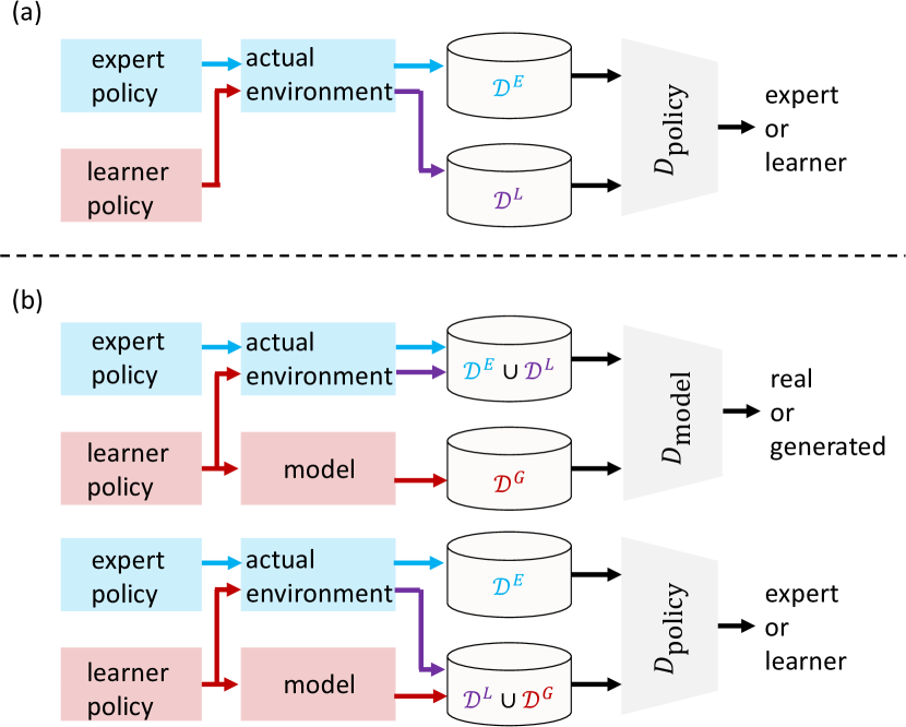
Figure 1: Comparison of available datasets and discriminators between model-free and model-based imitation learning: (a) Model-free setting: Expert dataset $\mathcal{D}^{E}$ and learner’s dataset $\mathcal{D}^{L}$ are created through interactions with actual environments. Policy discriminator $D_{\mathrm{policy}}$ exists. (b) Our proposed model-based setting: Simulated dataset $\mathcal{D}^{G}$ is additionally generated from learner’s policy and model. Two discriminators exist: $D_{\mathrm{model}}$ and $D_{\mathrm{policy}}$.

To further reduce the number of interactions with the actual environment, we propose Model-Based Entropy-Regularized Imitation Learning (MB-ERIL), which explicitly estimates a model of the environment and generates simulated data by running the learner’s policy in the estimated model. MB-ERIL is formulated as the minimization problem of Kullback-Leibler (KL) divergence between the expert policy evaluated in the actual environment and the learner’s policy evaluated in the model environment. MB-ERIL regularizes the policy and model by Shannon entropy and KL divergence to derive the algorithm, where we assume that the expert policy and the actual environment are solutions of the regularized Bellman equation.

The following are the contributions of this work:

• It develops two novel discriminators. One is a policy discriminator that differentiates actions generated by the policy from expert actions. The other is that a model discriminator that distinguishes the state transitions generated by the model from the actual transitions provided by an expert.

• The discriminators are represented by the reward, state, and state-action value functions. The value functions are updated by training the discriminators, a step that makes the forward RL efficient.

• For model fitting, MB-ERIL provides another objective alternative to maximum likelihood estimation.

• The estimated model generates counterfactual data to update the state and state-action value functions (Fig. 1(b)). As a result, we can reduce the number of costly interactions with the actual environment.

To evaluate MB-ERIL, we conducted two continuous control benchmark tasks in the MuJoCo simulator [10] and a vision-based reaching task [9] using a real upper-body humanoid robot. MB-ERIL shows promising experimental results with competitive asymptotic performance and higher sample efficiency than previous studies and empirically ensures low model bias, which is the gap between the actual environment and the model, by jointly updating the model and policy.

II LITERATURE REVIEW

II-A Model-free imitation learning

Relative Entropy Inverse RL [11] is a sample-based method inspired by Maximum entropy inverse RL (MaxEntIRL) [12]. It provides an efficient way of estimating the partition function of the probability distribution of expert trajectories. However, one drawback is utilizing a fixed sampling distribution, which is unhelpful in practice. Generative Adversarial Imitation Learning (GAIL) [2], which can adapt the sampling distribution using policy optimization, is closely related to GAN. GAIL is more sample efficient than Behavior Cloning (BC) with respect to the number of expert demonstrations. However, GAIL often requires many interactions with the environment because (1) an on-policy model-free forward RL is used for policy improvement and (2) the discriminator is not structured. Adversarial Inverse Reinforcement Learning (AIRL) [5] and Logistic Regression-based inverse RL [13] propose a structured discriminator represented by the reward and state-value functions, although an on-policy forward RL updates the policy. Adversarial Soft Advantage Fitting (ASAF) [14] exploits the discriminator inspired by the AIRL discriminator, although the state transition is not considered explicitly. To reduce the number of environmental interactions, an off-policy model-free forward RL has been adopted [6, 7, 15, 16]. We proposed Model-Free Entropy-Regularized Imitation Learning (MF-ERIL) based on entropy regularization that shares the network parameters between the discriminator and the generator. Even though MF-ERIL achieved better sample efficiency than the above methods, there is room to improve the sample efficiency by introducing model learning. MB-ERIL is one instantiation of this approach. Recent approaches corrected the issues around reusing data previously collected while training the discriminator [17, 18].

GAN-like imitation learning often suffers from unstable learning from adversarial training. Therefore, some regularization terms are added to BC’s loss function to stabilize the learning process. For example, Soft Q Imitation Learning (SQIL) is a regularized BC algorithm, where the squared soft Bellman error is used as a regularizer [19]. Interestingly, its algorithm can be implemented by assigning a reward of 1 to expert demonstrations and 0 to generated ones. Discriminator Soft Actor-Critic [20] is an extension of SQIL where its predefined reward value is replaced by the parameterized reward trained by the discriminator.

II-B Model-based imitation learning

MaxEntIRL, which is a pioneer of an entropy regularized RL, estimates the reward function from expert trajectories based on the maximum entropy principle. MaxEnt IRL is a model-based approach, although how to train the model was not discussed. Although a method was proposed that simultaneously estimated the reward and the model [21], maximum likelihood estimation was applied to model learning.

A few studies introduced model learning to GAIL to propagate the discriminator’s gradient to the policy for a gradient update. Consequently, Model-based GAIL [22, 23] and Model-based AIRL [24] achieved end-to-end training, although these methods do not sample state transitions from the model while unrolling the trajectories. However, these approaches do not use simulated experiences through interaction with the model, and therefore, they still require many actual interactions with a real environment [25]. Data-Efficient Adversarial Learning for Imitation from Observation (DEALIO), which is a GAIL-like algorithm [26], adopts a model-based RL that is employed for training a policy from the trained discriminator. Since one drawback of DEALIO is that model learning is independent of discriminator training, it suffers from model bias.

III PROPOSED METHOD

III-A Objective function

Consider Markov Decision Process (MDP) $\mathcal{M}=\langle\mathcal{X},\mathcal{U},p,r,\gamma\rangle$, where $\mathcal{X}$ denotes a continuous state space, $\mathcal{U}$ denotes an action space, $p:\mathcal{X}\times\mathcal{U}\times\mathcal{X}\mapsto\mathbb{R}_{\geq 0}$ denotes an actual stochastic state transition probability, $r:\mathcal{X}\mapsto\mathbb{R}$ denotes an immediate reward function, and $\gamma\in(0,1)$ denotes a discount factor that indicates how near and far future rewards are weighed. We chose the state-only function because more general reward functions like $r:\mathcal{X}\times\mathcal{U}\times\mathcal{X}\mapsto\mathbb{R}$ are often shaped as the result of training the discriminators. Let $b:\mathcal{X}\times\mathcal{U}\mapsto\mathbb{R}_{\geq 0}$ denote a stochastic policy to select action $\bm{u}\in\mathcal{U}$ at state $\bm{x}\in\mathcal{X}$. Let $\pi$ and $q$ denote an expert policy and a model of $p$. Note that $p$ and $\pi$ are unknown, while $q$ and $b$ are maintained by the learner.

MB-ERIL minimizes the following KL divergence:

$$J(q,b)=\mathbb{E}_{p^{L}(\bm{x},\bm{u},\bm{x}^{\prime})}\left[\ln\frac{p^{L}(\bm{x},\bm{u},\bm{x}^{\prime})}{p^{E}(\bm{x},\bm{u},\bm{x}^{\prime})}\right],$$

where $p^{L}$ and $p^{E}$ are respectively the joint density functions defined by

$$p^{L}(\bm{x},\bm{u},\bm{x}^{\prime}) =q(\bm{x}^{\prime}\mid\bm{x},\bm{u})b(\bm{u}\mid\bm{x})p^{L}(\bm{x}),$$

$$p^{E}(\bm{x},\bm{u},\bm{x}^{\prime}) =p(\bm{x}^{\prime}\mid\bm{x},\bm{u})\pi(\bm{u}\mid\bm{x})p^{E}(\bm{x}),$$

where $p^{L}(\bm{x})$ and $p^{E}(\bm{x})$ are some initial distributions, and we assume $p^{L}(\bm{x})=p^{E}(\bm{x})$ for simplicity. The difficulty is how to evaluate the log-ratio because it is unknown.

III-B Entropic regularization of policy and model

The basic idea for estimating the log-ratio is to adopt the density ratio trick [27]. Then MB-ERIL updates the policy and the model by minimizing the estimated KL divergence. To derive the algorithm, we formulate the entropic regularization of the policy and the model. We add two regularization terms to the immediate reward:

$$r(\bm{x})+\kappa^{-1}\mathcal{H}(p(\cdot\mid\bm{x},\bm{u})\pi(\cdot\mid\bm{x}))$$

$$\qquad-\eta^{-1}\mathrm{KL}(p(\cdot\mid\bm{x},\bm{u})\pi(\cdot\mid\bm{x})\parallel q(\cdot\mid\bm{x},\bm{u})b(\cdot\mid\bm{x})),$$

where $\mathcal{H}$ represents the operator of Shannon entropy, and $\kappa$ and $\eta$ denote positive hyperparameters.

Then the Bellman optimality equation is given by

$$V(\bm{x})=\max_{\pi}\mathbb{E}_{\pi}\left\{-\kappa^{-1}\ln\pi(\bm{u}\mid\bm{x})-\eta^{-1}\ln\frac{\pi(\bm{u}\mid\bm{x})}{b(\bm{u}\mid\bm{x})}\right.$$

$$\quad+\max_{p}\mathbb{E}_{p}\biggl{[}r(\bm{x})+\gamma V(\bm{x}^{\prime})$$

$$\quad\quad\left.-\kappa^{-1}\ln p(\bm{x}^{\prime}\mid\bm{x},\bm{u})-\eta^{-1}\ln\frac{p(\bm{x}^{\prime}\mid\bm{x},\bm{u})}{q(\bm{x}^{\prime}\mid\bm{x},\bm{u})}\biggr{]}\right\},$$ (1)

where $V(\bm{x})$ denotes a state-value function. To utilize the framework of entropic regularization, MB-ERIL assumes that $\pi(\bm{u}\mid\bm{x})$ and $p(\bm{x}^{\prime}\mid\bm{x},\bm{u})$ are the solutions of the Bellman equation (1) when the learner uses baseline policy $b(\bm{u}\mid\bm{x})$ and baseline state transition $q(\bm{x}^{\prime}\mid\bm{x},\bm{u})$. Using the Lagrangian multiplier method, we obtain the following equations:

$$p(\bm{x}^{\prime}\mid\bm{x},\bm{u})$$

$$\quad=\frac{\exp[\beta(r(\bm{x})+\gamma V(\bm{x}^{\prime})+\eta^{-1}\ln q(\bm{x}^{\prime}\mid\bm{x},\bm{u}))]}{\exp[\beta Q(\bm{x},\bm{u})]},$$ (2)

$$\pi(\bm{u}\mid\bm{x})=\frac{\exp[\beta(Q(\bm{x},\bm{u})+\eta^{-1}\ln b(\bm{u}\mid\bm{x}))]}{\exp(\beta V(\bm{x}))},$$ (3)

where $\beta$ is a positive hyperparameter defined by $\beta\triangleq\frac{\kappa\eta}{\kappa+\eta}$. $Q(\bm{x},\bm{u})$ denotes the state-action value function, and the following relation exists between $V$ and $Q$:

$$\exp(\beta Q(\bm{x},\bm{u}))=\int\exp\left[\beta(r(\bm{x})+\gamma V(\bm{x}^{\prime})\right.\\ \left.+\eta^{-1}\ln q(\bm{x}^{\prime}\mid\bm{x},\bm{u})\right]\mathrm{d}\bm{x}^{\prime},$$ (4)

$$\exp(\beta V(\bm{x}))=\int\exp\left[\beta(Q(\bm{x},\bm{u})+\eta^{-1}\ln b(\bm{u}\mid\bm{x}))\right]\mathrm{d}\bm{u}.$$ (5)

See Appendix A for the derivation.

III-C Derivation of MB-ERIL discriminators

We obtain the following equations from (2) and (3) that represent the density ratio:

$$\beta^{-1}\ln\frac{p(\bm{x}^{\prime}\mid\bm{x},\bm{u})}{q(\bm{x}^{\prime}\mid\bm{x},\bm{u})} =r(\bm{x})+\gamma V(\bm{x}^{\prime})-Q(\bm{x},\bm{u})$$

$$\quad-\kappa^{-1}\ln q(\bm{x}^{\prime}\mid\bm{x},\bm{u}),$$

$$\beta^{-1}\ln\frac{\pi(\bm{u}\mid\bm{x})}{b(\bm{u}\mid\bm{x})}=Q(\bm{x},\bm{u})-V(\bm{x})-\kappa^{-1}\ln b(\bm{u}\mid\bm{x}).$$

Using the density ratio estimation [27], we derive a model discriminator that distinguishes the state transition generated by the model from the real transitions provided by the expert:

$$D_{\mathrm{model}}(\bm{x}^{\prime}\mid\bm{x},\bm{u})$$

$$\quad=\frac{\exp(\beta f(\bm{x},\bm{u},\bm{x}^{\prime}))}{\exp(\beta f(\bm{x},\bm{u},\bm{x}^{\prime}))+\exp(\beta\kappa^{-1}\ln q(\bm{x}^{\prime}\mid\bm{x},\bm{u}))},$$

where $f(\bm{x},\bm{u},\bm{x}^{\prime})$ is defined by

$$f(\bm{x},\bm{u},\bm{x}^{\prime})\triangleq r(\bm{x})+\gamma V(\bm{x}^{\prime})-Q(\bm{x},\bm{u}).$$

Similarly, the policy discriminator is given by

$$D_{\mathrm{policy}}(\bm{u}\mid\bm{x})$$

$$\quad=\frac{\exp(\beta(Q(\bm{x},\bm{u})-V(\bm{x})))}{\exp(\beta(Q(\bm{x},\bm{u})-V(\bm{x})))+\exp(\beta\kappa^{-1}\ln b(\bm{u}\mid\bm{x}))},$$

which differentiates the action generated by the policy from the expert action. Note that $D_{\mathrm{policy}}$ is the discriminator used by AIRL and MF-ERIL if $Q(\bm{x},\bm{u})$ is replaced with $r(\bm{x})+\gamma V(\bm{x}^{\prime})$. These discriminators have the same form as the optimal discriminator, also known as the Bradley-Terry model [28].

III-D MB-ERIL learning

In the model-free setting, the learner needs to interact with a real environment to generate trajectories like the expert, making the model-free setting sample inefficient. On the other hand, the learner can generate trajectories by interacting with the real environment and the model. Learning from simulated trajectories is sometimes called Dyna architecture [29]. To improve the sample efficiency, we adopt Dyna architecture, and therefore, MB-ERIL utilizes the following three datasets. The first is an expert dataset generated by an expert in a real environment:

$$\mathcal{D}^{E}=\{(\bm{x}_{i},\bm{u}_{i},\bm{x}_{i}^{\prime})\}_{i=1}^{N^{E}},\quad\bm{x}_{i}\sim p_{0}^{E}(\cdot)\quad$$

$$\quad\bm{u}_{i}\sim\pi(\cdot\mid\bm{x}_{i}),\quad\bm{x}_{i}^{\prime}\sim p(\cdot\mid\bm{x}_{i},\bm{u}_{i}),$$

where $N^{E}$ is the number of transitions in the dataset and $p_{0}^{E}$ is the discounted state distribution [30] for ($\pi$, $p$). The second and third are the learner’s datasets by running $b(\bm{u}\mid\bm{x})$ in the real environment and the model:

$$\mathcal{D}^{L}=\{(\bm{x}_{i},\bm{u}_{i},\bm{x}_{i}^{\prime})\}_{i=1}^{N^{L}},\quad\bm{x}_{i}\sim p_{0}^{L}(\cdot)\quad$$

$$\quad\bm{u}_{i}\sim b(\cdot\mid\bm{x}_{i}),\quad\bm{x}_{i}^{\prime}\sim p(\cdot\mid\bm{x}_{i},\bm{u}_{i}),$$

$$\mathcal{D}^{G}=\{(\bm{x}_{i},\bm{u}_{i},\bm{x}_{i}^{\prime})\}_{i=1}^{N^{G}},\quad\bm{x}_{i}\sim q_{0}(\cdot)\quad$$

$$\quad\bm{u}_{i}\sim b(\cdot\mid\bm{x}_{i}),\quad\bm{x}_{i}^{\prime}\sim q(\cdot\mid\bm{x}_{i},\bm{u}_{i}),$$

where $N^{L}$ and $N^{G}$ are the dataset sizes, and $p_{0}^{L}$ and $q_{0}$ are the discounted state distributions for ($\pi^{L}$, $p$) and ($\pi^{L}$, $q$). Normally, $N^{G}\gg N^{L}\geq N^{E}$, because collecting data in the real environment is expensive.

Here we show MB-ERIL’s learning rules that consist of (1) training the discriminators, (2) policy evaluation, and (3) policy improvement. First, we show the loss functions for training $\mathcal{D}_{\mathrm{model}}$ and $\mathcal{D}_{\mathrm{policy}}$ to estimate $r$, $V$, and $Q$:

$$\mathcal{L}_{\mathrm{model}}(r,V,Q)=-\mathbb{E}_{(\bm{x},\bm{u},\bm{x}^{\prime})\sim\mathcal{D}^{E}\cup\mathcal{D}^{L}}\left[\ln D_{\mathrm{model}}(\bm{x}^{\prime}\mid\bm{x},\bm{u})\right]$$

$$\quad-\mathbb{E}_{(\bm{x},\bm{u},\bm{x}^{\prime})\sim\mathcal{D}^{G}}\left[\ln(1-D_{\mathrm{model}}(\bm{x}^{\prime}\mid\bm{x},\bm{u}))\right]$$

where $\mathbb{E}_{(\bm{x},\bm{u},\bm{x}^{\prime}\sim\mathcal{D})}$ represents the expectation over a batch of data that is uniformly sampled from an experience replay buffer $\mathcal{D}$. Similarly, the loss function for $D_{\mathrm{policy}}$ is given by

$$\mathcal{L}_{\mathrm{policy}}(V,Q)=-\mathbb{E}_{(\bm{x},\bm{u})\sim\mathcal{D}^{E}}\left[\ln D_{\mathrm{policy}}(\bm{u}\mid\bm{x})\right]$$

$$\quad-\mathbb{E}_{(\bm{x},\bm{u})\sim\mathcal{D}^{L}\cup\mathcal{D}^{G}}\left[\ln(1-D_{\mathrm{policy}}(\bm{u}\mid\bm{x}))\right].$$

Note that $r$, $V$, and $Q$ are all updated, and $q$ and $b$ remain fixed while training the discriminators. These two loss functions are summarized:

$$\mathcal{L}_{\mathrm{dis}}(r,V,Q)=\lambda_{\mathrm{model}}\mathcal{L}_{\mathrm{model}}(r,V,Q)\\ +\lambda_{\mathrm{policy}}\mathcal{L}_{\mathrm{policy}}(V,Q),$$ (6)

where $\lambda_{\mathrm{model}}$ and $\lambda_{\mathrm{policy}}$ denote positive hyperparameters. Training the discriminators is interpreted by an inverse RL because the reward function is estimated.

Next we show how the state and state-action value functions are updated. This corresponds to the policy evaluation step. Using (4) and (5), the following loss function can be constructed:

$$\mathcal{L}(V,Q)=\lambda_{QV}\mathbb{E}_{\bm{x},\bm{u}}\biggl{[}$$

$$\;\;\left(Q-\beta^{-1}\ln\mathbb{E}_{q}\left[\exp(\beta(r+\gamma V^{\prime}-\kappa^{-1}\ln q))\right]\right)^{2}\biggr{]}$$

$$\quad+\lambda_{VQ}\mathbb{E}_{\bm{x}}\left[\left(V-\beta^{-1}\ln\mathbb{E}_{b}\left[\exp(\beta(Q-\kappa^{-1}\ln b))\right]\right)^{2}\right],$$ (7)

where $\lambda_{QV}$ and $\lambda_{VQ}$ denote constant hyperparameters. We simplify the notation by omitting the arguments of the functions and setting $V^{\prime}\triangleq V(\bm{x}^{\prime})$ for readability. This loss function contains the log-expected-exponent terms, which introduce biases in their gradients [31]. Empirically, using a biased estimate was sufficient for our experiments, although applying Fenchel conjugates is also promising.

Finally, we explain how the model and policy are updated based on the trained discriminators in the policy improvement step. As Soft Actor-Critic does [32], they are directly learned by minimizing the expected KL divergence based on (2) and (3):

$$q(\bm{x}^{\prime}\mid\bm{x},\bm{u})\leftarrow\mathrm{arg}\min_{q^{\prime}}$$

$$\;\;\mathbb{E}_{\bm{x},\bm{u}}\left[\mathrm{KL}\left(q^{\prime}\parallel\frac{\exp[\beta(r+\gamma V^{\prime}+\eta^{-1}\ln q)]}{\exp[\beta Q]}\right)\right],$$ (8)

$$b(\bm{u}\mid\bm{x})\leftarrow\mathrm{arg}\min_{b^{\prime}}\mathbb{E}_{\bm{x}}\left[\mathrm{KL}\left(b^{\prime}\parallel\frac{\exp[\beta(Q+\eta^{-1}\ln b)]}{\exp(\beta V)}\right)\right].$$ (9)

MB-ERIL is summarized in Algorithm 1. Lines 7 and 8 correspond to learning from simulated trajectories like Dyna architecture.

Algorithm 1 Model-Based Entropy-Regularized Imitation Learning (MB-ERIL)

1:Expert dataset $\mathcal{D}^{E}$ and hyperparameters $\kappa$ and $\eta$

2:Learner’s policy $b$, model $q$, reward $r$, state-value $V$, and state-action value $Q$.

3:Initialize all parameters of networks and replay buffers $\mathcal{D}^{L},\mathcal{D}^{G}$.

4:(Pre-train the Regularized AutoEncoder using $\mathcal{D}^{E}$ when raw images are used as inputs.)

5:for $k=0,1,2,\ldots$ do

6:     $\triangleright$ Collect state transitions in the real environment and the model.

7:     $\mathcal{D}^{L}\leftarrow\mathcal{D}^{L}\cup\{(\bm{x}_{t},\bm{u}_{t},\bm{x}_{t+1})\}_{t=0}^{N^{L}}$ with $b$ and $p$.

8:     $\mathcal{D}^{G}\leftarrow\mathcal{D}^{G}\cup\{(\bm{x}_{t},\bm{u}_{t},\bm{x}_{t+1})\}_{t=0}^{N^{G}}$ with $b$ and $q$.

9:     $\triangleright$ Train the discriminators

10:     Update $r$, $V$, and $Q$ by minimizing (6).

11:     $\triangleright$ Evaluate policy $\qquad\hskip 123.76949pt.$

12:     $\mathcal{D}^{G}\leftarrow\mathcal{D}^{G}\cup\{(\bm{x}_{t},\bm{u}_{t},\bm{x}_{t+1})\}_{t=0}^{N^{G}}$ with $b$ and $q$.

13:     Update $V$ and $Q$ by minimizing (7).

14:     $\triangleright$ Improve the policy and the model $\qquad\hskip 79.09866pt.$

15:     Update $q$ and $b$. See (8) and (9).

16:end for

III-E Simplified MB-ERIL

Here we show two simplified MB-ERIL implementations by removing some components. One is MB-ERIL without training the discriminators, which trains $r$, $V$, and $Q$ by the maximum likelihood method instead of minimizing (6). The loss function is given by

$$\mathcal{L}^{\prime}(r,V,Q)=-\mathbb{E}_{\mathcal{D}^{E}}\left[\ln p(\bm{x}^{\prime}\mid\bm{x},\bm{u})\right]$$

$$\quad-\mathbb{E}_{\mathcal{D}^{E}}\left[\ln b(\bm{u}\mid\bm{x})\right]+\mathcal{L}(V,Q).$$ (10)

The first term of the right-hand side of (1) corresponds to model cloning, and the third term is the regularizer, which resembles SQIL. We call this approach Entropy-Regularized Model and Behavior Cloning (ERMBC).

The other is MB-ERIL without training the generator inspired by ASAF. This approach simply skips lines 7 and 8 of Algorithm 1, meaning that it does not learn from the additional simulated trajectories even though the model is maintained explicitly. We call this approach MB-ERIL without Policy Evaluation (MB-ERIL\PE).

IV MUJOCO BENCHMARK CONTROL TASKS

IV-A Task description

To verify our proposed method, we first conducted two benchmark control tasks, Ant and Humanoid, provided by OpenAI gym [33]. Both use a physics engine called MuJoCo [10]. The goal of these tasks is to move forward as quickly as possible. First, an optimal policy was trained by the Trust Region Policy Optimization [34], based on the original reward function provided by the simulator. Then it was used as an expert policy to collect expert data $\mathcal{D}^{E}$. We adopted the sparse sampling setup [8] in which we randomly sampled $(\bm{x},\bm{u},\bm{x}^{\prime})$ triplets from each trajectory.

The functions used by MB-ERIL need to be approximated by artificial neural networks, and $r(\bm{x})$, $V(\bm{x})$, $Q(\bm{x},\bm{u})$, and $b(\bm{u}\mid\bm{x})$ were represented by a two-layer neural network with a derivative of the sigmoid-weighted linear unit (dSiLU) [35] as an activation function, determined based on our previous study [9]. We defined the model to output a Gaussian distribution conditioned on the state and the action,i.e.: $q(\bm{x}^{\prime}\mid\bm{x},\bm{u})=\mathcal{N}(\bm{x}^{\prime}\mid\bm{\mu}(\bm{x},\bm{u}),\bm{\Sigma}(\bm{x},\bm{u}))$, where $\bm{\mu}(\bm{x},\bm{u})$ and $\bm{\Sigma}(\bm{x},\bm{u})$ denote the mean vector and the diagonal covariance matrix for simplicity. Future work will investigate more complicated distributions, such as a mixture of Gaussians with full covariance. Each was represented by a neural network with two hidden layers, and each layer had 256 nodes with dSiLU activations.

IV-B Comparative evaluation

We evaluated the MB-ERIL, ERMBC, and MB-ERIL\PE performances by comparing them with the following algorithms:

• Dyna-MF-ERIL: MF-ERIL [9] with the Dyna framework [29], which generates simulated trajectories by interacting with the model. The model, represented by a separate neural network, is trained by the simple maximum likelihood method. Then MF-ERIL is trained from real and generated data.

• MF-ERIL: We ignored the first discriminator that estimates $\ln p_{0}^{E}(\bm{x})/p_{0}^{L}(\bm{x})$ for simplicity.

• DAC: Discriminator-Actor-Critic (DAC) [7], which is baseline model-free imitation learning.

• BC: naive Behavior Cloning that minimizes the negative log-likelihood objective.

Following Ho and Ermon [2], a single trajectory contains 50 state-action transition pairs $(\bm{x},\bm{u},\bm{x}^{\prime})$, i.e., 50 steps per episode. The number of trajectories sampled from expert policy $\pi$ were set to 30 and 350 in the Ant and Humanoid environments. We set $N^{L}=10^{2}$ and $N^{G}=10^{4}$.

Fig. 2 compares the learning curves. Note that the reward functions estimated by each method cannot be directly compared since inverse reinforcement learning is an ill-posed problem. Therefore, the method was evaluated by the mean normalized return:

$$\bar{R}_{\mathrm{mean}}=\frac{1}{N}\sum_{i=1}^{N}\frac{R_{i}-R_{\min}}{R_{\max}-R_{\min}},$$

where $i$ is the index of the experimental run and $N$ is the number of experiments. $R_{i}$ is the raw return of the $i$-th experimental run, where the original reward of OpenAI gym was used. $R_{\min}$ and $R_{\max}$ are constants, where $R_{\max}$ is given by the return of the expert while $R_{\min}=0$. In the Ant environment, the maximum normalized total reward was reached by MB-ERIL, MF-ERIL, DAC, ERMBC, and MB-ERIL\PE in that order; Dyna-MF-ERIL and BC did not reach the expert performance. MB-ERIL improved the learning efficiency of the model-free methods (MF-ERIL and DAC) by about ten times. Note that the asymptotic performance of Dyna-MF-ERIL was worse than that of MF-ERIL even though the performing model did learn and its normalized return increased rapidly in the early stage of learning. Perhaps the model failed to learn the state transition because model learning by the maximum likelihood method cannot deal with a covariate shift. ERMBC and MB-ERIL\PE also converged to the expert performance, although they learned much slower than MF-ERIL. Similar results were obtained in the Humanoid environment. MB-ERIL learned faster than the other methods, although MF-ERIL and DAC eventually achieved comparable performance. The performance of MB-ERIL\PE was worst or inferior to BC.

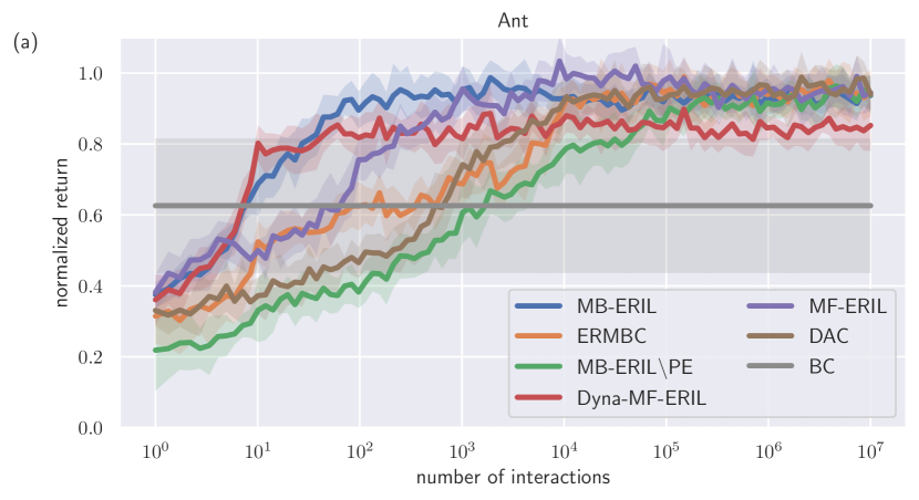
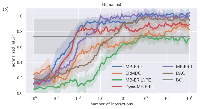
Figure 2: Normalized return versus number of interactions on MuJoCo benchmark control tasks: Solid lines represent average values, and shaded areas correspond to $\pm 1$ standard deviation region. Note that horizontal axis is a log scale.

Next we evaluated the data efficiency of the training discriminators by changing the number of samples in $\mathcal{D}^{E}$. Fig. 3 shows that MB-ERIL, MB-ERIL\PE, MF-ERIL, and DAC found policies that exhibited higher control performance with fewer expert demonstrations. On the other hand, ERMBC and Dyna-MF-ERIL just exhibited slight performance degradation when the number of demonstrations was limited, implying that model learning did not improve the sample efficiency with respect to the number of expert demonstrations. However, the MB-ERIl\PE performance was degraded in the Humanoid environment; it did not improve even though the number of demonstrations increased. The results indicate that $V$ and $Q$ did not satisfy the soft Bellman equations (4) and (5) when they were simply estimated by training the discriminators. We conclude that the policy evaluation of MB-ERIL was more crucial when the state space is large.

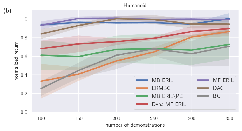
Figure 3: Normalized return versus number of trajectories provided by expert on MuJoCo benchmark control tasks

To see the model and policy differences among MB-ERIL, Dyna-MF-ERIL, and MF-ERIL, we computed the negative log-likelihood (NLL) of the finally-obtained model and policy using test expert data. For example, the model’s NLL was calculated by

$$\mathrm{NLL}=-\frac{1}{N_{\mathrm{test}}^{E}}\sum_{\ell=1}^{N_{\mathrm{test}}^{E}}\ln q(\bm{x}_{\ell}^{\prime}\mid\bm{x}_{\ell},\bm{u}_{\ell}),$$

where $N_{\mathrm{test}}^{E}$ is the number of samples in the test data. The policy’s NLL was defined similarly. Figs. 4(a) and (c) compare the NLLs of the policies on the MuJoCo experiments, showing no significant difference between the MB-ERIL and MF-ERIL policies, although Dyna-MF-ERIL’s NLL was larger than the others, which led to its poor asymptotic performance. Figs. 4(b) and (d) show that the NLL of the model obtained by MB-ERIL was the smallest among the other methods.

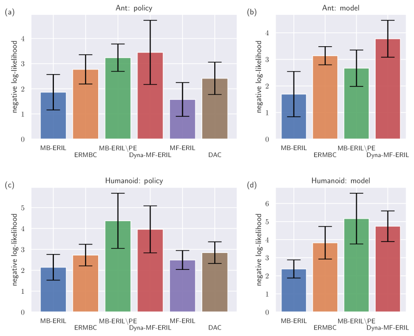
Figure 4: Comparison of NLL in Ant and Humanoid environments: Smaller is better because vertical axis is negative log-likelihood. (a) and (c) NLL of policy. (b) and (d) NLL of model. Note that MF-ERIL and DAC did not estimate the model.

V REAL ROBOT CONTROL

V-A Task description

Next we performed a vision-based reaching task [9] with an upper-body humanoid called Nextage developed by Kawada Industries Inc. Two colored blocks served as obstacles, and one switch button indicated the goal in the workspace. The aim is to move its left arm’s end-effector from a starting position (Fig. 5(a)) to a target position (Fig. 5(b)) as quickly as possible, where the starting and target positions were selected randomly from the pre-defined positions in Fig. 5(c). This task is more complicated than the FetchReach provided by OpenAI Gym because the target position must be detected from visual information. Nextage has a head with two cameras, a torso, two 6-axis manipulators, and two cameras attached to its end-effectors. We mounted cameras on its left arm and head in this task. The head pose was fixed during the experiments.

The state was given by $\bm{x}=[\theta_{1},\ldots,\theta_{6},\bm{z}^{\top}]^{\top}$, where $\theta_{i}$ is the $i$-th joint angle of the left arm and $\bm{z}$ represents the latent visual state obtained by a deterministic Regularized AutoEncoder (RAE) [36]. The action was given by the changes in the joint angle from previous position $\bm{u}=[\Delta\theta_{1},\ldots,\Delta\theta_{6}]^{\top}$, where $\Delta\theta_{i}$ is the change in the joint angle from the previous position of the $i$-th joint (although we clamped $\Delta\theta_{i}$ in $[-1,1]$. Figs. 5(d) and (e) show the entire network architecture that represents the functions and the RAE encoder whose input came from two $160\times 128$ RGB images captured by Nextage’s cameras.

We prepared several environmental configurations by changing the arm’s initial pose, the button’s location, and the height of the blocks. We designed three initial and two target poses for the expert configuration (Fig.5(c)). The learning configuration was given by five initial and two target poses. In addition, we prepared blocks of two different heights, resulting in $3\times 2\times 2=12$ expert configurations and $5\times 2\times 2=20$ learning configurations. We created expert demonstrations with MoveIt! [37] using the geometric information of the button and the colored blocks. Note that such information was unavailable for learning the algorithms. MoveIt! generated 12 trajectories for every expert configuration, and we sampled 50 transitions for each trajectory. Consequently, $N^{E}=12\times 50$ expert transitions were obtained. Although the sequence of the joint angles was almost deterministic, the RGB images were stochastic and noisy due to the lighting conditions. In this experiment, $N^{L}$ and $N^{G}$ were set to $20\times 50$ and $10^{4}$. On the other hand, the test configuration was constructed by one initial pose (red circle) and one target one (red square) that were not included in the expert and learner’s configurations.

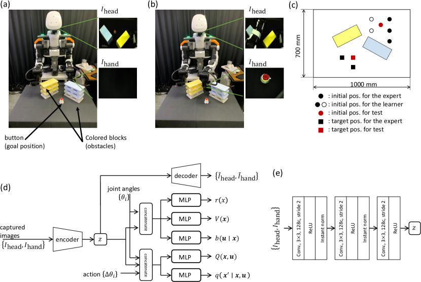
Figure 5: Vision-based reaching task: (a) Starting position. (b) Target position. (c) Possible environmental configuration. (d) Network architecture for reward, state value, policy, state-action value, and model. (e) Network architecture for encoder: Conv. denotes a convolutional neural network. “$n$c” denotes “$n$ channels.”

V-B Experimental results

We compared MB-ERIL with ERMBC, MB-ERIL\PE, Dyna-MF-ERIL, MF-ERIL, DAC, ASAF, and BC. We measured the performances by investigating a synthetic reward function: $r=\exp\left(-\frac{\|\bm{p}_{t}-\bm{p}_{g}\|_{2}^{2}}{\sigma^{2}}\right)$, where $\bm{p}_{t}$ and $\bm{p}_{g}$ denote the end-effector’s current and target position. Parameter $\sigma$ was set to 5.

To evaluate the performance during training, we evaluated the policy’s performance every ten episodes with a test set of initial and goal positions that were not included in the training demonstrations from the expert.

Fig. 6 compares the performance, where the horizontal and vertical axes represent the number of environmental interactions and normalized returns. MB-ERIL achieved higher sample efficiency than the other baselines. Unlike the MuJoCo experiments, Dyna-MF-ERIL was comparable to MF-ERIL, indicating that the model bias was not serious in this task. However, Dyna-MF-ERIL did not exploit the model efficiently because it did not improve the sample efficiency. Fig. 7 shows that the NLL of MB-ERIL’s policy was comparable to those of ERMBC, MB-ERIL\PE, MF-ERIL, and DAC, although the NLL of MB-ERIL’s model was the smallest.

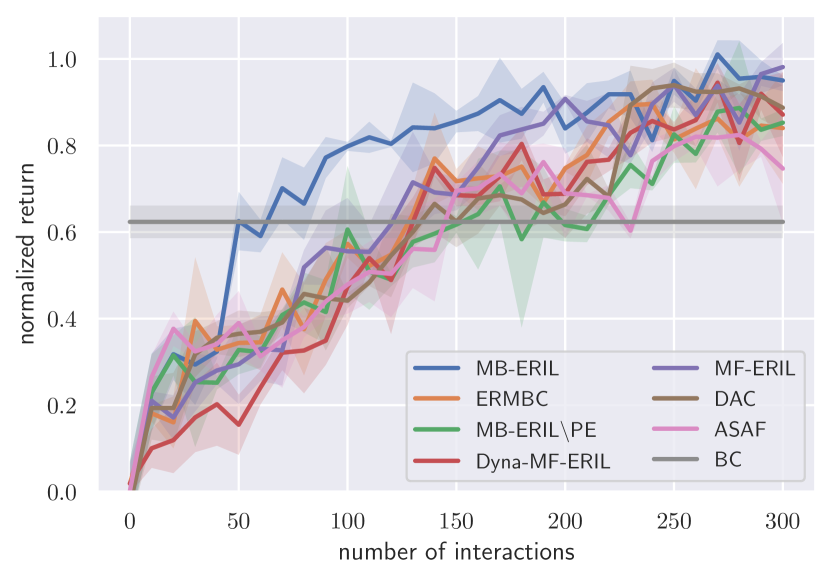
Figure 6: Normalized return versus number of interactions on Nextage vision-based reaching task

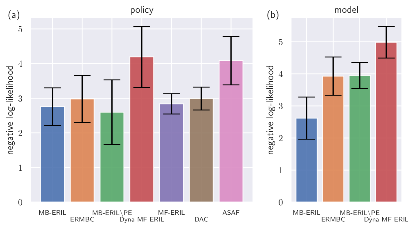
Figure 7: Comparison of NLL on Nextage vision-based reaching task: (a) Policy’s NLL and (b) Model’s NLL

VI CONCLUSIONS

We proposed MB-ERIL, derived from RL theory, which regularized the policy and the model. The experimental results of the simulated and real robots showed that MB-ERIL improved the sample efficiency over MF-ERIL, Dyna-MF-ERIL, DAC, and BC. A comparison between MB-ERIL and Dyna-MF-ERIL suggests that the simple use of data generated by the model was not useful due to the model bias. As explained in Section I, our formulation is based on the assumption that the expert policy and the actual environment are solutions of the regularized Bellman equation, although this assumption is not straightforward. In the future, we will provide a clear derivation of ERIL.

Our experimental results on the Ant task show that MB-ERIL’s asymptotic performance was slightly worse than that of MF-ERIL due to model bias. One possible solution is to switch the algorithm from MB-ERIL to MF-ERIL based on the loss function of the model discriminator. MB-ERIL updates $V$ and $Q$ alternatively with respect to two different objective functions. Although the update rules were derived from the Bellman equation (1), the convergence and stability were not proved theoretically. In future work, we will apply the technique used in the convergence proof of GAIL [38, 39].

APPENDIX

-A Derivation of (2) - (5)

Consider the maximization problem inside the right-hand side of (1). It is a constrained optimization because $\int p(\bm{x}^{\prime}\mid\bm{x},\bm{u})\mathrm{d}\bm{x}^{\prime}=1$. The Lagrangian is given by

$$\mathcal{L}_{2}=\int p\left(r-\kappa^{-1}p-\eta^{-1}\ln\frac{p}{q}+\gamma V^{\prime}\right)\mathrm{d}\bm{x}^{\prime}\\ +\lambda_{1}\left(1-\int p\mathrm{d}\bm{x}^{\prime}\right),$$ (11)

where $\lambda_{1}$ is the Lagrangian multipliers. Note that we simplified the notation here to improve its readability. We set the derivative with respect to $p$ to 0 and used the constraint to yield the following equation:

$$p=\frac{\exp[\beta(r+\gamma V^{\prime}+\eta^{-1}\ln q)]}{\exp(1+\beta\lambda_{1})},$$

where the denominator is given by

$$\exp(1+\beta\lambda_{1})=\int\exp[\beta(r+\gamma V^{\prime}+\eta^{-1}\ln q)\mathrm{d}\bm{x}^{\prime}.$$ (12)

By defining the right-hand side of (12) as $\exp\beta Q$, we obtain (2) and (4). Substituting the above results into (1) yields

$$V=\max_{\pi}\mathbb{E}_{\pi}\left[-\kappa^{-1}\ln\pi-\eta^{-1}\ln\frac{\pi}{b}+Q\right].$$

Similarly, we can maximize the right-hand side using the Lagrangian multipliers method and obtain (3) and (5).

References

- [1] C. Finn, P. Christiano, P. Abbeel, and S. Levine, “A connection between generative adversarial networks, inverse reinforcement learning, and energy-based models,” in NIPS 2016 Workshop on Adversarial Training, 2016.
- [2] J. Ho and S. Ermon, “Generative adversarial imitation learning,” in NeurIPS, 2016.
- [3] N. Ab Aza, A. Shahmansoorian, and M. Davoudi, “From inverse optimal control to inverse reinforcement learning: A historical review,” Annual Reviews in Control, vol. 50, pp. 119–138, 2020.
- [4] S. Arora and P. Doshi, “A survey of inverse reinforcement learning: Challenges, methods and progress,” Artificial Intelligence, 2021.
- [5] J. Fu, K. Luo, and S. Levine, “Learning robust rewards with adversarial inverse reinforcement learning,” in Proc. of ICLR, 2018.
- [6] L. Blondé and A. Kalousis, “Sample-efficient imitation learning via generative adversarial nets,” in Proc. of AISTATS, 2019.
- [7] I. Kostrikov, K. K. Agrawal, D. Dwibedi, S. Levine, and J. Tompson, “Discriminator-actor-critic: Addressing sample inefficiency and reward bias in adversarial imitation learning,” in Proc. of ICLR, 2019.
- [8] F. Sasaki, T. Yohira, and A. Kawaguchi, “Sample efficient imitation learning for continuous control,” in Proc. of ICLR, 2019.
- [9] E. Uchibe and K. Doya, “Forward and inverse reinforcement learning sharing network weights and hyperparameters,” Neural Networks, vol. 144, pp. 138–153, 2021.
- [10] E. Todorov, T. Erez, and Y. Tassa, “MuJoCo: A physics engine for model-based control,” in Proc. of IROS, 2012.
- [11] A. Boularias, J. Kober, and J. Peters, “Relative entropy inverse reinforcement learning,” in Proc. of AISTATS, 2011.
- [12] B. D. Ziebart, A. Maas, J. A. Bagnell, and A. K. Dey, “Maximum entropy inverse reinforcement learning,” in Proc. of AAAI, 2008.
- [13] E. Uchibe, “Model-free deep inverse reinforcement learning by logistic regression,” Neural Processing Letters, vol. 47, no. 3, pp. 891–905, 2018.
- [14] P. Barde, J. Roy, W. Jeon, J. Pineau, C. Pal, and D. Nowrouzezahrai, “Adversarial soft advantage fitting: Imitation learning without policy optimization,” in NeurIPS, 2020.
- [15] G. Zuo, K. Chen, J. Lu, and X. Huang, “Deterministic generative adversarial imitation learning,” Neurocomputing, pp. 60–69, 2020.
- [16] G. Zuo, Q. Zhao, K. Chen, J. Li, and D. Gong, “Off-policy adversarial imitation learning for robotic tasks with low-quality demonstrations,” Applied Soft Computing, 2020.
- [17] Z. Zhu, K. Lin, B. Dai, and J. Zhou, “Off-policy imitation learning from observations,” in NeurIPS, 2020.
- [18] H. Hoshino, K. Ota, A. Kanezaki, and R. Yokota, “OPIRL: Sample efficient off-policy inverse reinforcement learning via distribution matching,” in Proc. of ICRA, 2022.
- [19] S. Reddy, A. D. Dragan, and S. Levine, “SQIL: Imitation learning via regularized behavioral cloning,” in Proc. of ICLR, 2020.
- [20] D. Nishio, D. Kuyoshi, T. Tsuneda, and S. Yamane, “Discriminator soft actor critic without extrinsic rewards,” in Proc. of the 9th IEEE Global Conference on Consumer Electronics, 2020, pp. 327–32.
- [21] M. Herman, T. Gindele, J. Wagner, F. Schmitt, and W. Burgard, “Inverse reinforcement learning with simultaneous estimation of rewards and dynamics,” in Proc. of AISTATS, 2016.
- [22] N. Baram, O. Anschel, I. Caspi, and S. Mannor, “End-to-end differentiable adversarial imitation learning,” in Proc. of ICML, 2017.
- [23] N. Rhinehart, K. M. Kitani, and P. Vernaza, “R2P2: A ReparameteRized Pushforward Policy for diverse, precise generative path forecasting,” in Proc. of ECCV, 2018.
- [24] J. Sun, L. Yu, P. Dong, B. Lu, and B. Zhou, “Adversarial inverse reinforcement learning with self-attention dynamics model,” IEEE Robotics and Automation Letters, vol. 6, no. 2, pp. 1880–1886, 2021.
- [25] V. Saxena, S. Sivanandan, and P. Mathur, “Dyna-AIL: Adversarial imitation learning by planning,” in ICLR 2020 Workshop: Beyond Tabula Rasa in Reinforcement Learning, 2020.
- [26] F. Torabi, G. Warnell, and P. Stone, “DEALIO: Data-efficient adversarial learning for imitation from observation,” in Proc. of IROS, 2021.
- [27] M. Sugiyama, T. Suzuki, and T. Kanamori, Density ratio estimation in machine learning. Cambridge University Press, 2012.
- [28] R. A. Bradley and M. E. Terry, “Rank analysis of incomplete block designs: I. the method of paired comparisons,” Biometrika, vol. 50, no. 3/4, pp. 324–345, 1952.
- [29] R. S. Sutton, “Integrated architecture for learning, planning, and reacting based on approximating dynamic programming,” in Proc. of ICML, 1990.
- [30] R. S. Sutton, D. McAllester, S. Singh, and Y. Mansour, “Policy gradient methods for reinforcement learning with function approximation,” in NeurIPS, 2000, pp. 1057–1063.
- [31] I. Kostrikov, O. Nachum, and J. Tompson, “Imitation learning via off-policy distribution matching,” in Proc. of ICLR, 2019.
- [32] T. Haarnoja, A. Zhou, P. Abbeel, and S. Levine, “Soft Actor-Critic: Off-policy maximum entropy deep reinforcement learning with a stochastic actor,” in Proc. of ICML, 2018.
- [33] G. Brockman, V. Cheung, L. Pettersson, J. Schneider, J. Schulman, J. Tang, and W. Zaremba, “OpenAI Gym,” CoRR, abs/1606.01540, 2016.
- [34] J. Schulman, S. Levine, P. Abbeel, M. Jordan, and P. Moritz, “Trust region policy optimization,” in Proc. of ICML, 2015.
- [35] S. Elfwing, E. Uchibe, and K. Doya, “Sigmoid-weighted linear units for neural network function approximation in reinforcement learning,” Neural Networks, vol. 107, pp. 3–11, 2018.
- [36] P. Ghosh, M. S. M. Sajjadi, A. Vergari, M. Black, and B. Schaolkopf, “From variational to deterministic autoencoders,” in Proc. of ICLR, 2020.
- [37] S. Chitta, I. Sucan, and S. Cousins, “Moveit! [ROS topics],” IEEE Robotics Automation Magazine, vol. 19, no. 1, pp. 18–19, 2012.
- [38] Y. Zhang, Q. Cai, Z. Yang, and Z. Wang, “Generative adversarial imitation learning with neural networks: Global optimality and convergence rate,” in Proc. of ICML, 2020.
- [39] Z. Guan, X. Tengyu, and L. Yingbin, “When will generative adversarial imitation learning algorithms attain global convergence,” in Proc. of AISTATS, 2021.