Optimally Controllable Perceptual Lossy Compression

Abstract

Recent studies in lossy compression show that distortion and perceptual quality are at odds with each other, which put forward the tradeoff between distortion and perception (D-P). Intuitively, to attain different perceptual quality, different decoders have to be trained. In this paper, we present a nontrivial finding that only two decoders are sufficient for optimally achieving arbitrary (an infinite number of different) D-P tradeoff. We prove that arbitrary points of the D-P tradeoff bound can be achieved by a simple linear interpolation between the outputs of a minimum MSE decoder and a specifically constructed perfect perceptual decoder. Meanwhile, the perceptual quality (in terms of the squared Wasserstein-2 distance metric) can be quantitatively controlled by the interpolation factor. Furthermore, to construct a perfect perceptual decoder, we propose two theoretically optimal training frameworks. The new frameworks are different from the distortion-plus-adversarial loss based heuristic framework widely used in existing methods, which are not only theoretically optimal but also can yield state-of-the-art performance in practical perceptual decoding. Finally, we validate our theoretical finding and demonstrate the superiority of our frameworks via experiments. Code is available at: https://github.com/ZeyuYan/Controllable-Perceptual-Compression

1 Introduction

Lossy compression is an essential technique for digital data storage and transport. For decades, the goal of lossy compression is to achieve the lowest possible distortion at a given bit rate, which is bounded by Shannon’s rate-distortion function (Shannon, 1959; Cover & Thomas, 2006). However, recent studies show that typical distortion measures, e.g., MSE, PSNR and SSIM/MS-SSIM (Wang et al., 2003; Zhou Wang et al., 2004), are not fully consistent with human’s subjective judgement on perceptual quality (Johnson et al., 2016; Zhang et al., 2018; Blau & Michaeli, 2018). The work (Blau & Michaeli, 2018) lays a first theoretical foundation for understanding the distortion-perception (D-P) tradeoff, revealing that distortion and perception quality are at odds with each other. It accords well with empirical results that improving perceptual quality by adversarial learning and/or deep features based perceptual loss would lead to an increase of the distortion (Galteri et al., 2017; M Tschannen, 2018; Santurkar et al., 2018; Agustsson et al., 2019; Iwai et al., 2020; Mentzer et al., 2020; Ohayon et al., 2021; Prakash et al., 2021).

For lossy compression, the “classic” rate-distortion theory has been recently expanded in (Blau & Michaeli, 2019) to take the perceptual quality into consideration, resulting in a rate-distortion-perception three-way tradeoff. Using a divergence from the source distribution to measure the perceptual quality, the monotonicity and convexity of the rate-distortion-perception function have been established. More recently, (Yan et al., 2021) shows that an optimal encoder for the “classic” rate-distortion problem is also optimal for the perceptual compression problem with perception constraint. Hence, a minimum MSE (MMSE) encoder is universal for perceptual lossy compression. In light of this, to obtain different perceptual quality, a natural way is to use a fixed MMSE encoder whilst train different decoders to fulfill different D-P tradeoff (Zhang et al., 2021).

In this paper, we present a nontrivial theoretical finding that it is unnecessary to train different decoders for different perceptual quality, and two specifically constructed decoders are enough for achieving arbitrary D-P tradeoff. Furthermore, we propose two optimal training frameworks for perfect perceptual decoding to enable the realization of this kind of convenient D-P tradeoff.

In summary, our contributions are as follows:

• A theoretical finding for optimal D-P tradeoff in lossy compression. We prove that, with distortion measured by squared error and perceptual quality measured by squared Wasserstein-2 distance, arbitrary points of the D-P tradeoff bound can be achieved by a simple linear interpolation between an MMSE decoder and a specifically constructed perceptual decoder with perfect perception constraint. Besides, in theory the perceptual quality (measured in terms of squared Wasserstein-2 distance) can be quantitatively controlled by the interpolation factor. This finding reveals that two specifically constructed and paired decoders are sufficient for optimally achieving arbitrary (an infinite number of different) D-P tradeoff.

• Two optimal training frameworks for perfect perceptual decoding, which enables the realization of interpolation based optimal D-P tradeoff. One of them trains a perceptual decoder to decode directly from compressed representation with the aid of an MMSE decoder. The other uses a combination structure consists of an MMSE encoder-decoder pair followed by a post-processing perceptual decoder. While the former has a more compact structure, the latter is more flexible that applies to existing lossy compression systems optimized only in terms of distortion measures. Particularly, while existing frameworks depend heavily on the VGG loss and hence are only effective on RGB images, our frameworks do not suffer from this limitation and are effective for arbitrary data.

• Experiments on MNIST, depth images and RGB images, which validate our theoretical finding and demonstrate the performance of our frameworks. We show that the proposed frameworks are not only theoretically optimal but also can practically achieve state-of-the-art perceptual quality.

It is worth noting that an optimal training framework for perfect perceptual decoding has been recently proposed in (Yan et al., 2021), which only uses a single conditioned adversarial loss to train a perceptual decoder. Though theoretically optimal and has shown superiority on MNIST, it struggles to yield satisfactory performance on data with more complex distribution, e.g., RGB images. This is due to the fact that in practice adversarial loss only is insufficient for stable training of a decoder to decode RGB images from compressed representation. We augment the framework of (Yan et al., 2021) by additionally conditioning on an MMSE decoder. We prove that this augmentation does not compromise the optimality. Hence our frameworks are still optimal for training perfect perceptual decoder, and, more importantly, can achieve satisfactory performance on RGB images.

After completing this paper and when about to submit it for publication, we became aware of (Freirich et al., 2021), who prove that, for MSE distortion and Wasserstein-2 perception index, optimal estimators on the D-P curve can be interpolated from the estimators at the two extremes of the D-P curve, e.g., an MMSE estimator and a perfect perception estimator. This result is similar to our result in property ii) of Theorem 1. However, our result is fundamentally different from that in (Freirich et al., 2021) as follows: 1) Compared with the restoration problem considered in (Freirich et al., 2021), the lossy compression problem in this work requires jointly optimizing an encoder and a decoder, hence is more involved. 2) Our analysis (proof of Theorem 1 ii)) is fundamentally different from (Freirich et al., 2021) not only in that we have to jointly consider an encoder and a decoder in the D-P tradeoff formulation, but also our analysis follows a completely different line, e.g., by analyzing the optimal solution of an unconstrained form of the D-P formulation (see Appendix A for details). 3) Besides, we propose an augmented optimal formulation for perfect perceptual decoding learning and further propose two optimal training frameworks for D-P controllable lossy compression.

2 Related Works

2.1 Perceptual Lossy Compression

In learning based image compression, a common way to improve perceptual quality is to incorporate an adversarial loss and/or a perceptual loss. Adversarial loss is typically implemented using generative adversarial networks (GAN) (Goodfellow et al., 2014), whilst perceptual loss computes a distance on deep features (Johnson et al., 2016; Simonyan & Zisserman, 2015; Gatys et al., 2016; Chen & Koltun, 2017; Dosovitskiy & Brox, 2016), e.g., MSE on the middle layers of the VGG net (Simonyan & Zisserman, 2015). Due to its high effectiveness in minimizing the divergence between distributions, adversarial learning has shown remarkable effectiveness in achieving high perceptual quality (Rippel & Bourdev, 2017; Agustsson et al., 2019; Ledig et al., 2017; Wang et al., 2018; Wu et al., 2020; Mentzer et al., 2020). Using a combination of distortion loss and adversarial loss, the D-P tradeoff can be controlled by the balance parameter between these two losses. However, simply combining distortion and adversarial losses is not optimal for perceptual decoding and D-P tradeoff. Besides, it needs to train different models for different D-P tradoff. (Yan et al., 2021) proposes an optimal training framework which uses an MMSE encoder and train a perfect perceptual decoder using adversarial training. Though can theoretically achieve the optimal condition of perfect perceptual decoding and has shown superiority on MINIST data, only using adversarial loss cannot obtain satisfactory performance on data with more complex distribution, e.g., RGB images.

2.2 Distortion-Perception Tradeoff

While it is both theoretically and empirically demonstrated that distortion and perceptual quality are at odds with each other (Blau & Michaeli, 2018, 2019), it is unclear how to optimally and flexibly achieve arbitrary D-P tradeoff. The work (Yan et al., 2021) proves that the lossy compression problem with or without perception constraint can share a same encoder, but it is limited to perfect perception constraint. Traditional methods using a combination of distortion loss, adversarial loss and deep features based loss can control the D-P tradeoff by adjusting the balance parameters between the losses. But for different perceptual quality (i.e. different D-P tradeoff), different encoder-decoder pairs need to be trained. (Zhang et al., 2021) further shows that the D-P tradeoff can be achieved by fixing an MMSE encoder and varying the decoder to (approximately) achieve any point along the D-P tradeoff. Even though it only requires to train a single encoder, different decoders need to be trained for different D-P tradeoff. (Iwai et al., 2020) considers the tradeoff between distortion and fidelity by interpolating the parameters or the outputs of two decoders. However, the method is heuristic and not optimal.

3 Theory for Optimally Controllable D-P Tradeoff

3.1 Perceptual Lossy Compression

In lossy compression, the goal is to represent data with less bits and reconstruct data with low distortion (Toderici et al., 2016; Agustsson et al., 2017; Toderici et al., 2017; Li et al., 2018; Mentzer et al., 2018; Minnen et al., 2018; Guo et al., 2021) or high perceptual quality (Rippel & Bourdev, 2017; Agustsson et al., 2019; Ledig et al., 2017; Wang et al., 2018; Wu et al., 2020; Iwai et al., 2020; Mentzer et al., 2020). Recent studies have revealed that distortion and perceptual quality are at odds with each other. More specifically, high perceptual quality can only be achieved with some necessary increase of the lowest achievable distortion. Hence, a tradeoff between distortion and perception has to be considered (Blau & Michaeli, 2018). For the lossy compression problem, this has been recently taken into consideration by extending the classic rate-distortion tradeoff theory to the rate-distortion-perception three-way tradeoff (Blau & Michaeli, 2019; Matsumoto, 2018, 2019).

The perceptual quality of a decoded sample refers to the degree to which it looks like a natural sample from human’s perception (subjective judgments), regardless its similarity to the reference source sample. A natural way to quantify perceptual quality in practice is to conduct real-versus-fake questionnaire studies (Zhang et al., 2018, 2016; Salimans et al., 2016). Conforming with this common practice, it can be mathematically defined in terms of the deviation between the statistics of decoded outputs and natural samples. For instance, denote the source and decoded output by $X$ and $\hat{X}$, respectively, the perceptual quality of $\hat{X}$ can be conveniently defined as (Blau & Michaeli, 2018)

$$d(p_{X},p_{\hat{X}}),$$ (1)

where $d(\cdot,\cdot)$ is a deviation measure between two distributions, such as the KL divergence or Wasserstein distance. Such a definition correlates closely with human subjective score and accords well with the principles of no-reference image quality measures (Mittal et al., 2013a; Wang & Simoncelli, 2005).

With these understanding, a natural way to achieve perceptual decoding is to promote the decoded outputs to have a distribution as close as possible to that of natural samples. In practice, this can be implemented by incorporating an adversarial loss into training to use a distortion-plus-adversarial loss (DAL) as

$$L=\lambda L_{adv}+L_{dis},$$ (2)

where $L_{dis}$ is a distortion loss such as MSE, $\ell_{1}$ norm, or distance between deep features, which computes the distortion between the reconstruction and its paired reference source. $L_{adv}$ is an adversarial loss responsible for minimizing the deviation from the distribution of natural samples to promote high perceptual quality. $\lambda>0$ is a balance parameter. Loss (2) and its many variants are widely used for achieving high perceptual quality and have shown remarkable effectiveness in fulfilling that goal (Rippel & Bourdev, 2017; Agustsson et al., 2019; Ledig et al., 2017; Wang et al., 2018; Wu et al., 2020; Iwai et al., 2020; Mentzer et al., 2020).

Though have shown good effectiveness, such methods have limitations as explained as follows. To achieve perfect perceptual quality, $d(p_{X},p_{\hat{X}})\leq 0$ (i.e. $p_{X}=p_{\hat{X}}$) is desired. Formulation (2) relaxes the constraint $d(p_{X},p_{\hat{X}})\leq 0$ by incorporating it with a distortion loss to get an unconstrained form. This relaxation eases the implementation, e.g., (2) can be implemented by a GAN and MSE loss in practice, but it cannot achieve perfect (or near perfect) perceptual quality with $d(p_{X},p_{\hat{X}})\leq 0$. Even though a very large value of $\lambda$ would promote $d(p_{X},p_{\hat{X}})$ to get close to 0, in this case the distortion cannot be well optimized and would result in undesirable excessive increase in distortion (Yan et al., 2021). In Section 4, we propose two theoretically optimal training frameworks that do not suffer from such limitations.

With (2), the distortion and perceptual quality of a compression system (i.e., D-P tradeoff) can be controlled by adjusting the value of $\lambda$. Intuitively, to attain different D-P tradeoff, different models have to be trained for different values of $\lambda$. Next, we show that only two specifically constructed decoders are enough for optimally achieving arbitrary D-P tradeoff.

3.2 Theoretical Results for Optimally Controllable D-P Tradeoff

When using the DAL framework (2) to achieve different D-P tradeoff, not only different models have to be trained but also it is not theoretically optimal. Here we present a theoretical result for optimal D-P tradeoff with only two decoders.

For a given bit-rate $R$, let $X$ be the source and $(E,G)$ be an encoder-decoder pair. When distortion is measured by MSE and perceptual quality is measured by squared Wasserstein-2 distance, the D-P tradeoff can be expressed as

$$\begin{split}D(P):=&\mathop{\min}\limits_{E\in\Omega,G}\ \mathbb{E}{\left\|{X-G(E(X))}\right\|^{2}}\\ &{\rm{s.t.}}~{}~{}~{}\ W^{2}_{2}({p_{X}},{p_{G(E(X))}})\leq P,\end{split}$$ (3)

where $W^{2}_{2}(\cdot,\cdot)$ is squared Wasserstein-2 distance, and $\Omega$ is the set of encoders, of which the average bit-rate is $R$.

When $P\!=\!+\infty$, (3) degenerates to the classic MMSE formulation without considering perceptual quality, as the constraint is invalid in this case. Accordingly, $D(\infty)$ is the lowest achievable MSE. When $P\!=\!0$, the system is enforced to yield perfect perceptual quality, with $D(0)$ being the lowest achievable MSE under perfect perception constraint. $D(P)$ is nonincreasing and convex (Blau & Michaeli, 2018), which satisfies $D(0)\!=\!2D(+\infty)$ (Yan et al., 2021).

We now state the result that a linear interpolation between the outputs of two optimal decoders under (3) with $P=+\infty$ and $P=0$, respectively, can achieve any points of the D-P tradeoff bound $D(P)$.

Theorem 1. Let $(E_{d},G_{d})$ be an optimal encoder-decoder pair to (3) when $P\!=\!+\infty$, and $G_{p}$ be an optimal decoder to (3) for a fixed encoder $E_{d}$ and $P\!=\!0$. Denote $Z_{d}:=E_{d}(X)$ and $P_{d}:=W^{2}_{2}(p_{X},p_{G_{d}(Z_{d})})$. Then, these hold:
i) $E_{d}$ is an optimal encoder to (3) for any $P\geq 0$.
ii) Let $\alpha=\min(\sqrt{P/P_{d}},1)\in[0,1]$, define

$$G^{*}_{\alpha}(Z_{d}):=\alpha G_{d}(Z_{d})+(1-\alpha)G_{p}(Z_{d}),$$

then $(E_{d},G^{*}_{\alpha})$ is an optimal encoder-decoder pair to (3).

When $P\geq P_{d}$, it is obvious that $\alpha=1$ and $(E_{d},G^{*}_{\alpha})=(E_{d},G_{d})$ is optimal to (3) as it reaches the lowest achievable MSE distortion $D(+\infty)=P_{d}=W^{2}_{2}(p_{X},p_{G_{d}(Z_{d})})$. Meanwhile, from the definition that $G_{p}$ is an optimal decoder to (3) for a fixed MMSE encoder $E_{d}$ when $P=0$, and by the results in (Yan et al., 2021), we have $\alpha=0$ and that $(E_{d},G^{*}_{\alpha})=(E_{d},G_{p})$ is optimal to (3) when $P=0$. Thus, to prove Theorem 1, we only need to consider the case of $0\!<\!P\!<\!P_{d}$. Consider an unconstrained formulation corresponding to (3) as

$$\begin{split}\mathop{\min}\limits_{E\in\Omega,G}\ &\alpha\mathbb{E}{\left\|X\!-\!G(E(X))\right\|^{2}}+(1\!-\!\alpha)W^{2}_{2}({p_{X}},{p_{G(E(X))}}),\end{split}$$ (4)

where $0<\alpha<1$. To prove Theorem 1, we first prove that $(E_{d},G^{*}_{\alpha})$ is an optimal encoder-decoder pair to (4), and then prove that, for any $0<P<P_{d}$, $(E_{d},G^{*}_{\alpha})$ with $\alpha=\min(\sqrt{P/P_{d}},1)$ is also optimal to (3). The details of proof are given in Appendix A.

Remark 1. Theorem 1 indicates that, for any $P\geq 0$, an optimal decoder $G^{*}_{\alpha}$ to (3) can be easily obtained by interpolating between an MMSE decoder $G_{d}$ and a perfect perceptual decoder $G_{p}$. Hence, it is unnecessary to train different decoders for different D-P tradeoff. A simple linear interpolation between the outputs of the two decoders $G_{d}$ and $G_{p}$ is enough to reach any points of the D-P bound $D(P)$. Furthermore, for an optimal encoder-decoder pair $(E_{d},G^{*}_{\alpha})$, the decoding distortion is

$$\begin{split}&\mathbb{E}{\|{X-(\alpha X_{d}+(1-\alpha)X_{p})}\|^{2}}\\ \mathop{\rm{=}}\limits^{(a)}&\mathbb{E}{\|{X_{d}-X}\|^{2}}+\mathbb{E}{\left\|{X_{d}-(\alpha X_{d}+(1-\alpha)X_{p})}\right\|^{2}}\\ \mathop{\rm{=}}\limits^{(b)}&[1+(1-\alpha)^{2}]\mathbb{E}{\left\|{X_{d}-X}\right\|^{2}}.\end{split}$$ (5)

where $X_{d}=G_{d}(E_{d}(X))$ and $X_{p}=G_{p}(E_{d}(X))$. The proof of step (a) is given in Appendix A, and (b) is due to $\mathbb{E}{\|{X_{d}-X_{p}}\|^{2}}=\mathbb{E}{\|{X_{d}-X}\|^{2}}$ (Yan et al., 2021). By varying the value of the interpolation factor $\alpha\in[0,1]$, we can control the tradeoff between the distortion and perceptual quality of decoding. When $\alpha=0$, the decoding distortion is exactly twice of that when $\alpha=1$, which is consistent with the result in (Yan et al., 2021).

Remark 2. Theorem 1 also implies that, an MMSE encoder is universal for perceptual lossy compression in that it is optimal under any perception constraint, e.g., $\forall P\geq 0$ in (3). (Yan et al., 2021) has proved that when distortion is measured by MSE, an MMSE encoder is also optimal under perfect perception constraint (i.e. $P=0$ in (3)). Our result expands this property to any $P\geq 0$, when perceptual quality is measured by squared Wasserstein-2 distance.

Remark 3. From Theorem 1, we can further draw some properties on the D-P tradeoff function $D(P)$. Specifically, when $P=+\infty$, we have

$$\begin{split}P_{d}=\mathop{\min}\limits_{p_{X,Z}}\mathbb{E}{\left\|{G_{d}(Z)-X}\right\|^{2}}=D_{d},\end{split}$$ (6)

where $D_{d}$ is the lowest achievable MSE distortion, i.e., the distortion of an optimal MMSE encoder-decoder pair. From (5) and (23) in Appendix A, the relationship between distortion $D$ and perception $P$ is

$$\begin{split}&D=D_{d}+(1-\alpha)^{2}D_{d},\\ &P=\alpha^{2}P_{d}=\alpha^{2}D_{d}.\end{split}$$ (7)

The first and second derivatives of $P$ with respect to $D$ are given by

$$\begin{split}\frac{dP}{dD}=&\frac{\alpha}{\alpha-1},\\ \frac{d^{2}P}{dD^{2}}=&\frac{1}{2(1-\alpha)^{3}D_{d}}.\end{split}$$ (8)

Then, it is easy to see that $\frac{dP}{dD}<0$ and $\frac{d^{2}P}{dD^{2}}>0$, $\forall\alpha\in(0,1)$. This is consistent with (Blau & Michaeli, 2019) that the D-P tradeoff is nonincreasing and convex.

It is worth noting from Theorem 1 that, to achieve interpolation based optimal D-P tradeoff, the MMSE decoder and the perfect perception decoder should be paired with a common MMSE encoder. Next we consider the construction of such decoders.

4 Optimal Training Frameworks for Perfect Perceptual Decoding

To realize the interpolation based D-P tradeoff as stated in Theorem 1, an MMSE decoder $G_{d}$ and a perfect perceptual decoder $G_{p}$ (both paired with a common MMSE encoder $E_{d}$) are needed. The encoder-decoder pair $(E_{d},G_{d})$ can be straightforwardly obtained via MMSE training. Meanwhile, the decoder $G_{p}$ can be trained by the framework in (Yan et al., 2021), which is theoretically optimal for perfect perceptual decoding. It is proved that the mapping of an optimal encoder-decoder pair with perfect perceptual quality is symmetric. The optimal condition is that the source $X$ and decoded output $\hat{X}$ have a same distribution conditioned on the compressed representation $Z$ as

$${p_{\hat{X}|Z}}={p_{X|Z}}.$$ (9)

This can be fulfilled by a two-stage training procedure (Yan et al., 2021): firstly train an encoder-decoder pair $(E_{d},G_{d})$ via minimizing MSE as

$$\mathop{\min}\limits_{E\in\Omega,G}\mathbb{E}\left\|X-G(E(X))\right\|^{2},$$ (10)

then fix the encoder $E_{d}$ and train a perceptual decoder $G_{p}$ by

$$\mathop{\min}\limits_{{p_{\hat{X},Z_{d}}}}W_{1}(p_{\hat{X},Z_{d}},p_{X,Z_{d}}),$$ (11)

where $Z_{d}:=E_{d}(X)$, $W_{1}$ is the Wasserstein-1 distance, which is implemented by WGAN with a conditional discriminator (Mirza & Osindero, 2014) to discriminate between $(\hat{X},Z_{d})$ and $(X,Z_{d})$.

Since distortion loss is not used in training $G_{p}$, the practical performance depends heavily on adversarial training. Although this framework has shown superiority over the DAL framework on MNIST, intensive experiments show that adversarial loss only (e.g. (11)) cannot yield satisfactory performance on RGB images.

4.1 An Augmented Optimal Formulation for Perfect Perceptual Decoding Learning

To address the limitation of the above framework, here we augment it to achieve satisfactory practical performance on RGB images, but without compromising its optimality. We propose an augmented formulation of (11) as

$$\mathop{\min}\limits_{{p_{\hat{X},X_{d}}}}W_{1}(p_{\hat{X},X_{d}},p_{X,X_{d}})+\lambda\mathbb{E}\|\hat{X}-X_{d}\|,$$ (12)

where $X_{d}:=G_{d}(E_{d}(X))$ with $(E_{d},G_{d})$ being a given MMSE encoder-decoder pair, $\lambda$ is a positive parameter associated with the augmentation term. Intuitively, formulation (12) incorporates an additional supervision provided by the $\ell_{2}$ distance from the MMSE decoding $X_{d}$, which is expected to assist the adversarial training.

Next, we prove that this augmentation does not change the optimal solution of (11), i.e., it is still optimal for perfect perceptual decoding learning. The proof is given in Appendix B.

Theorem 2. Let $(E_{d},G_{d})$ be an MMSE encoder-decoder pair, and $W_{1}(\cdot,\cdot)$ be the Wasserstein-1 distance. Denote $Z_{d}=E_{d}(X)$ and $X_{d}=G_{d}(Z_{d})$, then these hold:

• When $0\leq\lambda<1$, the optimal solution of (12) satisfies $p_{\hat{X},X_{d}}=p_{X,X_{d}}$, or equivalently $p_{\hat{X},Z_{d}}=p_{X,Z_{d}}$.

• When $\lambda>1$, the optimal solution of (12) satisfies $\hat{X}=X_{d}$.

Remark 4. Theorem 2 implies that, with any $\lambda\in[0,1)$, formulation (12) can achieve the optimal condition $p_{\hat{X},Z_{d}}=p_{X,Z_{d}}$ (equivalently $p_{\hat{X},X_{d}}=p_{X,X_{d}}$) for perfect perception decoding. Hence, it is still optimal for perfect perception decoding. In practice, the augmentation term is very helpful to enhance the training of the perceptual decoder, as will be shown in experiments. This benefit is mainly thanks to the fact that the augmentation term, which provides strong supervision by the $\ell_{2}$ distance from the MMSE decoding $X_{d}$, can effectively stabilize the training procedure.

Remark 5. Theorem 2 provides a solid theoretical foundation for the augmented formulation (12) that its solution satisfies the optimal condition for any $\lambda\in[0,1)$. However, to yield satisfactory performance in practical applications, the value of $\lambda$ still needs to be tuned. This is due to the facts that: 1) in practical implementation the Wasserstein-1 distance can only be approximated, e.g., by WGAN which involves 1-Lipschitz approximation (Ishaan et al., 2017); 2) the capacity of a decoding model (e.g., a deep network) in practice is not infinite. Thus, different values of $\lambda\in[0,1)$ would yield different practical performance, as illustrated in Table 2 in Appendix D. Another empirical illustration of Theorem 2 on MNIST is given in Figure 2.

4.2 Proposed Optimal Training Frameworks

(a) Framework A

(b) Framework B

Figure 1: Proposed optimal training frameworks for perfect perceptual decoding which applies to interpolation based D-P tradeoff.

Based on the above theoretical results, we propose two frameworks for perfect perceptual decoding training, which have different characteristics that may be discriminatively preferred in different applications.

The first is illustrated in Figure 1(a), which consists an MMSE encoder-decoder pair $(E_{d},G_{d})$ and a perfect perceptual decoder $G_{p}$ paired with $E_{d}$. The two decoders are separately trained by two steps: firstly train $(E_{d},G_{d})$ by the MSE loss, then fix the encoder to $E_{d}$ and train $G_{p}$ via (12). In the second step, (12) can be implemented by WGAN-gp (Ishaan et al., 2017), with the $\ell_{2}$ loss being incorporated into the adversarial loss of WGAN-gp to train $G_{p}$ and a discriminator $J$ alternatively. From Theorem 2, when using $\lambda<1$, the optimal condition for perfect perceptual decoding would be reached when $(G_{p},J)$ are trained to be optimal.

The second is illustrated in Figure 1(b), which has a combination structure consists of an MMSE encoder-decoder pair $(E_{d},G_{d})$ followed by a post-processing perceptual decoder $G_{p}$. It also involves two steps that firstly train an MMSE encoder-decoder pair $(E_{d},G_{d})$ and then train $G_{p}$ for post perceptual mapping from the output of $G_{d}$. That is $G_{p}$ is also trained via (12) but with $\hat{X}=G_{p}(G_{d}(E_{d}(X)))$.

In theory, both frameworks can optimally achieve arbitrary points of the D-P bound (3) by simply interpolating between $G_{d}$ and $G_{p}$ according to Theorem 1. While Framework A is straightforward and has a more compact structure, Framework B is more flexible that applies to any existing lossy compression system that optimized only in terms of decoding distortion. As will be shown in experiments (Appendix C), the MMSE encoder-decoder pair $(E_{d},G_{d})$ in Framework B can be replaced by an compression system only optimizing decoding distortion, e.g., BPG.

Note that in (3) and Theorem 1, the perceptual quality is measured by squared Wasserstein-2 distance, while here we use Wasserstein-1 distance for perfect perceptual decoding training (see (12)). This does not affect the optimality of the proposed frameworks when used for interpolation based D-P tradeoff, since Theorem 1 only requires $G_{p}$ to satisfy the optimal condition $P_{\hat{X},Z_{d}}\!=\!P_{{X},Z_{d}}$ (equivalently $P_{\hat{X},X_{d}}\!=\!P_{{X},X_{d}}$), regardless it is achieved by Wasserstein-1 distance, Wasserstein-2 distance, or any other divergence.

5 Experiments

We provide experiment results on MNIST, depth and RGB images. First, we verify Theorem 2 on MNIST (Lecun et al., 1998) by examining the effect of $\lambda$ in (12). Then, we evaluate the proposed frameworks on depth and RGB images. For both Framework A and B, $E_{d}$, $G_{d}$ are set the same as HiFiC (Mentzer et al., 2020). For framework A, the generator $G_{p}$ uses a convolutional layer to convert the encoded representation into a matrix with the same shape as the input images. The rest structure is set the same as the post-processing decoder in Framework B. For Framework B, the generator (post-processing decoder) has an U-net architecture, which consists of two down-sampling layers and two up-sampling layers with the use of residual channel attention block (RCAB) (Zhang et al., 2018; Wang et al., 2022). Skip connection is used to learn the residual. The discriminator has one more down-sampling layer than that in (Ledig et al., 2017) because the patch size is $128\times 128$.

5.1 Results on MNIST

Figure 2: Empirical decoding distortion of Framework A versus $\beta$ ($\lambda$ in (12) is related to $\beta$ in (13) as $\lambda=\frac{1-\beta}{\beta}$).

(a) Results of the traditional DAL framework (2) with different values of $\lambda$.

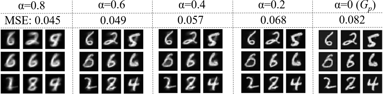
(b) Results interpolated between $G_{d}$ and $G_{p}$, i.e., $X_{\alpha}$ in (14). $G_{p}$ is trained by the proposed Framework A.

Figure 3: Typical sample comparison between the traditional DAL framework (2) and the proposed Framework A on MNIST.

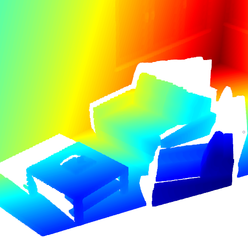
(a) Ground-truth (depth and its corresponding point cloud)

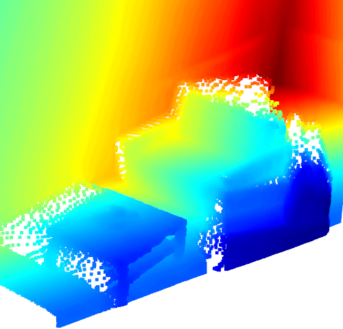
(b) $G_{d}$ (MMSE)

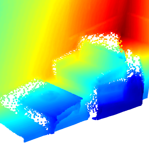
(c) $G_{h}$ (HiFiC)

(d) $G_{p}$ ($\alpha$=0)

(e) $\alpha$=0.25

(f) $\alpha$=0.5

(g) $\alpha$=0.75

Figure 4: Results on a sample from SUNCG dataset. (a) Ground-truth depth image and the corresponding point cloud. (b)-(d) Point cloud reconstructed from $G_{d}$, HiFiC and $G_{p}$. (e)-(g) Interpolated results between $G_{d}$ and $G_{p}$. For visual clarity, point cloud results are shown.

We train 20 compression models by Framework A for a bit-rate of 4, with the networks same as that in (Yan et al., 2021). For a fixed encoder $E_{d}$ trained by MMSE, we train the decoder $G_{p}$ using WGAN-gp (Ishaan et al., 2017) by

$$\begin{split}&\mathop{\max}\limits_{\left\|J\right\|_{L}\leq 1}\mathbb{E}[J(G_{p}(E(X)),E(X))]-\mathbb{E}[J(X,E(X))]\\ &\mathop{\min}\limits_{{G_{p}}}(1-\beta)\mathbb{E}{\left\|{G_{p}(X)-X_{d}}\right\|}-\beta\mathbb{E}[J(G_{p}(X),E(X))],\end{split}$$ (13)

where $J$ is a discriminator lies within the space of 1-Lipschitz functions, $X_{d}$ is the output of an MMSE encoder-decoder pair, $\beta$ is a balance parameter related to $\lambda$ in (12) as $\lambda=\frac{1-\beta}{\beta}$. Theorem 2 implies that the MSE of $G_{p}$ is the same as $G_{d}$ when $\beta<0.5$, but would double when $\beta>0.5$. Thus, in theory there would be a jump of the MSE at $\beta=0.5$ from $D(+\infty)$ (MSE of $G_{d}$) to $2D(+\infty)$ (double the MSE of $G_{d}$).

Figure 2 shows the empirical MSE of Framework A versus $\beta$. The theoretical jumping property can be (approximately) observed. As explained in Remark 5, the practical performance is related to the value of $\lambda$. Figure 3 shows the D-P tradeoff by interpolating the outputs of $G_{d}$ and $G_{p}$ as

$$X_{\alpha}={\alpha}G_{d}(E_{d}(X))+(1-\alpha)G_{p}(E_{d}(X)).$$ (14)

As expected, as $\alpha$ varying from 0 to 1, the decoding output becomes more blurry but has lower distortion. In Figure 3, the traditional DAL framework (2) (with different $\lambda$) is also compared. Clearly, for a similar MSE distortion result, the output of our framework is more clear.

5.2 Results on Depth Images

We further provide results on the SUNCG dataset (Song et al., 2017). For depth image compression, we use the post-processing framework, i.e. Framework B as shown in Figure 1(b). We first pretrain an encoder-decoder pair $(E_{d},G_{d})$ for 100 epochs by MMSE with regime set as ‘low’. Then our generator $G_{p}$ is trained by (12) with $\lambda=0.005$. For comparison, we train the HiFiC model for 100 epochs using the same hyper-parameters as in (Mentzer et al., 2020), denoted by $G_{h}$. Figure 4 shows the decoding results on a depth image. For visual clarity, we show the point cloud results reconstructed from the depth results. For MMSE decoding, the edges are blurry, resulting in a large amount of noisy points around edges in the point cloud result. Besides, the output of $G_{h}$ contains many noisy points around edges, which is even not distinctly better than that of the MMSE decoding. The perceptual quality of $G_{p}$ is much better, as shown in Figure 4(d). This is thanks to that the generator can well learn the distribution of clean depth images. For the interpolated results by (14), as $\alpha$ increases, the quality of point cloud degrades with the edges becoming more blurry.

As the proposed Framework B applies to any existing compression system that optimized only under certain distortion measure, an illustration of applying it to post-process the BPG codec is provided in Appendix C.

5.3 Results on RGB Images

Table 1: Perception score comparison on the KODAK dataset in two bit-rate conditions.

	Low (0.13 bpp)		High (0.41 bpp)
Methods	PSNR	PI	PSNR	PI
GT	$\infty$	2.23	$\infty$	2.23
$G_{d}$ (MMSE)	38.36	4.54	40.22	3.11
$G_{h}$ (HiFiC)	37.94	2.10	39.98	2.24
Framework A
$\alpha=0$ ($G_{p}$)	36.89	2.05	38.71	2.16
$\alpha=0.25$	37.45	2.18	39.28	2.15
$\alpha=0.50$	37.94	2.47	39.78	2.29
$\alpha=0.75$	38.27	3.32	40.13	2.73
Framework B
$\alpha=0$ ($G_{p}$)	36.87	2.08	38.60	2.18
$\alpha=0.25$	37.42	2.20	39.18	2.18
$\alpha=0.50$	37.90	2.48	39.71	2.32
$\alpha=0.75$	38.24	3.33	40.09	2.73

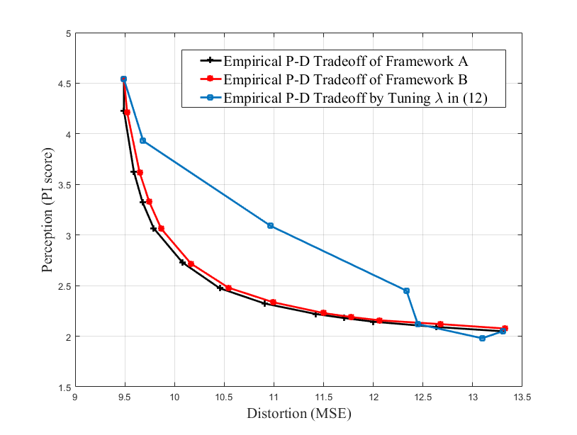
Figure 5: Empirical results on interpolation based perception-distortion tradeoff on the KODAK dataset.

In the experiment on RGB images, the networks are set the same as the depth image experiment, except the input channel number is 3 and $\lambda=0.01$. We train $G_{d}$, $G_{p}$, $G_{h}$ on COCO2014 (Lin et al., 2014) in two different bit-rates, with regime set as ‘low’ and ‘high’, and interpolate the outputs of $G_{d}$ and $G_{p}$ by (14) for D-P tradeoff. The perceptual quality is evaluated in terms of PI score (Blau et al., 2018), which is calculated by NIQE (Mittal et al., 2013b) and a learned network (Ma et al., 2017). As shown in Table LABEL:perceptiontable, the perception scores of $G_{p}$ outperforms HiFiC $G_{h}$ but with higher distortion. For each the proposed frameworks, as $\alpha$ increases, the distortion decreases but the PI score deteriorates. However, the perception score of HiFiC is better than the interpolated results of both the new frameworks when $\alpha=0.5$, with similar distortion. This is because our theorem result is derived on squared Wasserstein-2 distance. We also plot the empirical perception-distortion curve in Figure 5, including interpolated results by the two proposed frameworks, in comparison with the perception-distortion curve yielded by tuning $\lambda$ in (12). Since the samples in KODAK contains only 24 images, we use the PI score as perception measure rather than squared Wasserstein-2 distance. The perception-distortion curve of Framework A is similar to that of Framework B.

RGB samples for qualitative visual comparison are provided in Appendix D, see Figure 7-9. Moreover, both of the proposed frameworks outperform the networks trained by directly altering $\lambda$. The experimental details and the effect of the parameter $\lambda$ on the practical performance of Framework A is evaluated in Appendix D, see Table LABEL:lambdatable and Figure 10 in Appendix D.

6 Conclusion

We presented a theoretical finding for the D-P tradeoff problem in lossy compression that, two specifically constructed decoders are enough for arbitrary D-P tradeoff. We proved that arbitrary points of the D-P tradeoff bound can be achieved by simply interpolating between an MMSE decoder and a perfect perceptual decoder. Furthermore, we proposed two theoretically optimal training frameworks for perfect perceptual decoding. Experiments on MNIST, depth images and RGB images well verified our theoretical results and demonstrated the effectiveness of the proposed frameworks.

Taken together, this work lays a theoretical foundation for not only simply achieving optimal D-P tradeoff in lossy compression but constructing optimal training frameworks for perfect perceptual decoding that goes beyond existing heuristic frameworks.

Appendix A Proof of Theorem 1.

This section gives the proof of Theorem 1. When $P\geq P_{d}$, it is obvious that $\alpha=1$ and $(E_{d},G^{*}_{\alpha})=(E_{d},G_{d})$ is optimal to (3) as it reaches the lowest achievable MSE distortion $D(+\infty)=P_{d}=W^{2}_{2}(p_{X},p_{G_{d}(Z_{d})})$. Meanwhile, since $G_{p}$ is an optimal decoder to (3) for a fixed MMSE encoder $E_{d}$ when $P=0$, by the results in (Yan et al., 2021) we have $\alpha=0$ and that $(E_{d},G^{*}_{\alpha})=(E_{d},G_{p})$ is optimal to (3) when $P=0$. Thus, to prove Theorem 1, we only need to consider the case of $0<P<P_{d}$. Next, we first prove that $(E_{d},G^{*}_{\alpha})$ is an optimal encoder-decoder pair to (4), which is an unconstrained formulation of (3). Then, we prove that $(E_{d},G^{*}_{\alpha})$ is also an optimal encoder-decoder pair to (3) by analyzing the relationship between the optimal solutions of (3) and (4).

Denote $Z:=E(X)$, and consider an MMSE decoder $G_{1}(Z):=\mathbb{E}[X|Z]$, the first term of (4) can be expressed as

$$\begin{split}\mathbb{E}{\left\|{X-G(Z)}\right\|^{2}}=&\mathbb{E}{\left\|{X-G_{1}(Z)+G_{1}(Z)-G(Z)}\right\|^{2}}\\ =&\mathbb{E}{\left\|{X-G_{1}(Z)}\right\|^{2}}+\mathbb{E}{\left\|{X_{1}-G(Z)}\right\|^{2}}\\ &+2\mathbb{E}{\left\langle X-G_{1}(Z),X_{1}-G(Z)\right\rangle}\\ \mathop{\rm{=}}\limits^{(a)}&\mathbb{E}{\left\|{X-G_{1}(Z)}\right\|^{2}}+\mathbb{E}{\left\|{G_{1}(Z)-G(Z)}\right\|^{2}},\end{split}$$ (15)

where $<\cdot,\cdot>$ denotes the inner product, and $(a)$ is due to

$$\begin{split}&\mathbb{E}{\left\langle X-G_{1}(Z),G_{1}(Z)-G(Z)\right\rangle}\\ =&\mathbb{E}\{\mathbb{E}[\left\langle X-G_{1}(Z),G_{1}(Z)-G(Z)\right\rangle|G_{1}(Z)]\}\\ =&\mathbb{E}\{\mathbb{E}[(X-G_{1}(Z))|G_{1}(Z)]\cdot\mathbb{E}[G_{1}(Z)-G(Z)|G_{1}(Z)]\}\\ =&\mathbb{E}\{0\cdot\mathbb{E}[G_{1}(Z)-G(Z)|G_{1}(Z)]\}=0.\end{split}$$ (16)

Now, we first find an optimal decoder to (4) for a fixed encoder $E:X\to Z$, of which the joint distribution is denoted by $p_{X,Z}$. Denote $\hat{X}:=G(Z)$, the decoding mapping $G$ in (4) can be expressed as $p_{Z,\hat{X}}$. To avoid symbol confusion, we consider an auxiliary variable $X^{\prime}$ which has the same distribution as $X$, i.e. $p_{X^{\prime}}=p_{X}$, hence $W^{2}_{2}(p_{X^{\prime}},p_{\hat{X}})=W^{2}_{2}(p_{X},p_{\hat{X}})$. Then, from (15) and the fact that $\mathbb{E}{\left\|{X-G_{1}(Z)}\right\|^{2}}$ only depends on the encoder $E$, formulation (4) with a fixed encoder $E$ can be written as

$$\begin{split}&\mathop{\min}\limits_{p_{Z,\hat{X}}}\ \alpha\mathbb{E}{\|{\hat{X}-G_{1}(Z)}\|^{2}}+(1-\alpha)W^{2}_{2}({p_{X^{\prime}}},{p_{\hat{X}}})\\ =&\mathop{\min}\limits_{p_{Z,\hat{X}}}\alpha\mathbb{E}{\|{\hat{X}-G_{1}(Z)}\|^{2}}+\mathop{\min}\limits_{p_{X^{\prime},\hat{X}}}\ (1-\alpha)\mathbb{E}{\|{X^{\prime}-\hat{X}}\|^{2}}\\ =&\mathop{\min}\limits_{p_{X^{\prime},Z,\hat{X}}}\alpha\mathbb{E}{\|{\hat{X}-G_{1}(Z)}\|^{2}}+(1-\alpha)\mathbb{E}{\|{X^{\prime}-\hat{X}}\|^{2}}\\ =&\mathop{\min}\limits_{p_{X^{\prime},Z}}\mathop{\min}\limits_{p_{\hat{X}|X,Z}}\ \alpha\mathbb{E}{\|{\hat{X}-G_{1}(Z)}\|^{2}}+(1-\alpha)\mathbb{E}{\|{X^{\prime}-\hat{X}}\|^{2}},\end{split}$$ (17)

where $X^{\prime}$ is constrained by $P_{X^{\prime}}=P_{X}$. To find the optimal mapping $Z\to\hat{X}$ of (17), we first find the optimal solution of $\hat{X}$ when fixing $Z$ and $X^{\prime}$, and then find the distribution of $X^{\prime}$ conditioned on $Z$. Firstly, given $Z$ and $X^{\prime}$, it is easy to see that any optimal $\hat{X}$ to (17), denoted by $\hat{X}^{*}$, satisfies

$$\mathbb{E}[2\alpha(\hat{X}^{*}-G_{1}(Z))+2(1-\alpha)(\hat{X}^{*}-X^{\prime})]=0.$$ (18)

Therefore, given $Z$ and $X^{\prime}$, the optimal $p_{\hat{X}|X^{\prime},Z}$ to (17) satisfies

$$\hat{X}^{*}=\alpha G_{1}(Z)+(1-\alpha)X^{\prime}.$$ (19)

Then, substituting $\hat{X}=\hat{X}^{*}$ into (17), it follows that

$$\begin{split}&\mathop{\min}\limits_{p_{Z,\hat{X}}}\ \alpha\mathbb{E}{\|{\hat{X}-G_{1}(Z)}\|^{2}}+(1-\alpha)W^{2}_{2}({p_{X^{\prime}}},{p_{\hat{X}}})\\ =&\alpha(1-\alpha)\mathop{\min}\limits_{p_{X^{\prime},Z}}\mathbb{E}{\left\|{G_{1}(Z)-X^{\prime}}\right\|^{2}}\\ \geq&\alpha(1-\alpha)\mathbb{E}{\left\|{X_{d}-X}\right\|^{2}},\end{split}$$ (20)

where the last inequality is due to that $X_{d}=G_{d}(E_{d}(X))$ with $(E_{d},G_{d})$ being an MMSE encoder-decoder pair as defined in Theorem 1. Now, we find an optimal encoder to (4) given $\hat{X}^{*}$. From (20), formulation (4) can be written as

$$\begin{split}&\mathop{\min}\limits_{E\in\Omega}\ [\alpha\mathbb{E}{\left\|{G_{1}(E(X))-X}\right\|^{2}}+\alpha(1-\alpha)\mathop{\min}\limits_{p_{X^{\prime},E(X)}}\mathbb{E}{\left\|{G_{1}(E(X))-X^{\prime}}\right\|^{2}}]\\ \geq&\alpha\mathbb{E}{\left\|{X_{d}-X}\right\|^{2}}+\alpha(1-\alpha)\mathbb{E}{\left\|{X_{d}-X}\right\|^{2}}\\ =&\alpha(2-\alpha)\mathbb{E}{\left\|{X_{d}-X}\right\|^{2}}.\end{split}$$ (21)

Obviously, when $E=E_{d}$ and $p_{X^{\prime},E(X)}=p_{X,Z_{d}}$, the equality in (21) holds. Hence, the MMSE encoder $E_{d}$ is optimal to (4) for any $\alpha\in(0,1)$.

Next, we consider a fixed encoder $E_{d}$ to show that $G^{*}_{\alpha}$ is an optimal decoder to (4) for a fixed encoder $E_{d}$. When the encoder is fixed to $E_{d}$, from the definition of $(E_{d},G_{d})$, $X_{d}=G_{d}(E_{d}(X))$ and $G_{1}(Z)=\mathbb{E}[X|Z]$, we have $G_{1}(E_{d}(X))=G_{d}(E_{d}(X))=X_{d}$. Then it follows from (19) that

$$\hat{X}^{*}=\alpha X_{d}+(1-\alpha)X^{\prime},$$

with $X^{\prime}$ satisfying $p_{X^{\prime},Z_{d}}=p_{X,Z_{d}}$. Since the perfect perception decoder $G_{p}$ satisfies $p_{X_{p},Z_{d}}=p_{X,Z_{d}}$ (Yan et al., 2021), which means that $X^{\prime}$ can be replaced by $X_{p}$ and it follows that

$$\hat{X}^{*}=\alpha X_{d}+(1-\alpha)X_{p},$$

is an optimal decoder to (4) for fixed encoder $E_{d}$. Therefore, with $Z_{d}=E_{d}(X)$, $X_{d}=G_{d}(E_{d}(X))$ and $X_{p}=G_{p}(E_{d}(X))$, $G^{*}_{\alpha}(Z_{d})=\alpha G_{d}(Z_{d})+(1-\alpha)G_{p}(Z_{d})$ is an optimal decoder to (4). That is $(E_{d},G^{*}_{\alpha})$ is an optimal encoder-decoder pair to (4).

Now we prove that the encoder-decoder pair $(E_{d},G^{*}_{\alpha})$ is also optimal to (3). Taking $G^{*}_{\alpha}$ back into (20) we have

$$\begin{split}&\alpha\mathbb{E}{\left\|{G^{*}_{\alpha}(Z_{d})-G_{d}(Z_{d})}\right\|^{2}}+(1-\alpha)W^{2}_{2}({p_{X}},{p_{G^{*}_{\alpha}(Z_{d})}})\\ &=\alpha(1-\alpha)\mathop{\min}\limits_{p_{X,Z_{d}}}\mathbb{E}{\left\|{G_{d}(Z_{d})-X}\right\|^{2}}\\ &=\alpha(1-\alpha)P_{d},\end{split}$$ (22)

where $P_{d}=W^{2}_{2}(p_{X},p_{G_{d}(Z_{d})})$ as defined in Theorem 1. It follows from (22) that

$$W^{2}_{2}({p_{X}},{p_{G^{*}_{\alpha}(Z_{d})}})=\alpha^{2}P_{d}.$$ (23)

Thus, with $\alpha=\sqrt{P/P_{d}}$ for any $0\!<\!P\!<\!P_{d}$, and for a fixed encoder $E_{d}$, the optimal decoder $G^{*}_{\alpha}$ of (4) satisfies

$$W^{2}_{2}(p_{X},p_{G^{*}_{\alpha}(Z_{d})})=P.$$ (24)

Consider $0<P<P_{d}$ in (3), and let $(E^{\bullet},G^{\bullet})$ be any optimal encoder-decoder pair to (3), then, with (24), for $\alpha=\sqrt{P/P_{d}}$ we have

$$\mathbb{E}{\left\|{X-G^{\bullet}(E^{\bullet}(X))}\right\|^{2}} \leq\mathbb{E}{\left\|{X-G^{*}_{\alpha}(E_{d}(X))}\right\|^{2}},$$ (25)

$$W^{2}_{2}(p_{X},p_{G^{\bullet}(E^{\bullet}(X))}) \leq P=W^{2}_{2}(p_{X},p_{G^{*}_{\alpha}(E_{d}(X))}).$$ (26)

Summing up (25) and (26) yields

$$\begin{split}&\alpha\mathbb{E}{\left\|{X-G^{\bullet}(E^{\bullet}(X))}\right\|^{2}}+(1-\alpha)W^{2}_{2}(p_{X},p_{G^{\bullet}(E^{\bullet}(X))})\\ \leq&\alpha\mathbb{E}{\left\|{X-G^{*}_{\alpha}(E_{d}(X))}\right\|^{2}}+(1-\alpha)W^{2}_{2}(p_{X},p_{G^{*}_{\alpha}(E_{d}(X))}).\end{split}$$ (27)

Since $(E_{d},G^{*}_{\alpha})$ is an optimal encoder-decoder pair to (4), the equality in (27) holds. Hence, the equalities in (25) and (26) holds for any $(E^{\bullet},G^{\bullet})$, and $(E_{d},G^{*}_{\alpha})$ is an optimal solution to (3). This completes the proof of Theorem 1.

Appendix B Proof of Theorem 2.

Denote $Y\!:=\!(X,X_{d})$, $\hat{Y}\!:=\!(\hat{X},X_{d})$ and $Y_{d}\!:=\!(X_{d},X_{d})$, with which (12) can be rewritten as

$$\mathop{\min}\limits_{{p_{\hat{Y},Y_{d}}}}W_{1}(p_{\hat{Y}},p_{Y})+\lambda\mathbb{E}\|\hat{Y}-Y_{d}\|.$$ (28)

Then, to justify Theorem 2 i), it is enough to justify that, when $0\leq\lambda<1$, the optimal solution of (28) satisfies $p_{\hat{Y}}=p_{Y}$. Let $p^{*}_{\hat{Y},Y_{d}}$ be an optimal solution to (28), of which the optimal decoding output is $\hat{Y}^{*}$ and denote $\hat{Y}^{*}\!:=\!(\hat{X}^{*},X_{d})$. Then $p^{*}_{\hat{Y},Y_{d}}$ is also optimal to

$$\mathop{\min}\limits_{{p_{\hat{Y},Y_{d}}}}\mathbb{E}\|\hat{Y}-Y_{d}\|,~{}~{}~{}~{}{\rm{s.t.}}~{}~{}~{}~{}{p_{\hat{Y}}}={p_{\hat{Y}^{*}}},$$ (29)

which implies $\mathbb{E}\|\hat{Y}^{*}-Y_{d}\|=W_{1}(p_{\hat{Y}^{*}},p_{Y_{d}})$. Thus, the minimal objective value of (28) is

$$\begin{split}L^{*}=&W_{1}(p_{\hat{Y}^{*}},p_{Y})+\lambda W_{1}(p_{\hat{Y}^{*}},p_{Y_{d}})\\ \mathop{\rm{\geq}}\limits^{(a)}&(1-\lambda)W_{1}(p_{\hat{Y}^{*}},p_{Y})+\lambda W_{1}(p_{Y_{d}},p_{Y})\\ \mathop{\rm{\geq}}\limits^{(b)}&\lambda W_{1}(p_{Y_{d}},p_{Y}).\end{split}$$ (30)

In (a) we use the property of Wasserstein distance and (b) is because of the non-negativity of $(1-\lambda)W_{1}(p_{\hat{Y}^{*}},p_{Y})$. When $p_{\hat{Y}}=p_{Y}$, we have $W_{1}(p_{\hat{Y}^{*}},p_{Y})=0$ and $L^{*}=\lambda W_{1}(p_{Y_{d}},p_{Y})$. The equality of (b) holds if and only if $W_{1}(p_{\hat{Y}^{*}},p_{Y})=0$, which implies that the minimal objective is attained only when $p_{\hat{Y}^{*}}=p_{Y}$. Thus, $p_{\hat{Y}^{*}}=p_{Y}$ holds for any optimal solution $p^{*}_{\hat{Y},Y_{d}}$ of (28). This leads to the result that, for any $0\leq\lambda<1$, the optimal solution of (12) satisfies $p_{\hat{X},X_{d}}=p_{X,X_{d}}$.

Next, we further justify that the optimal condition $p_{\hat{X},X_{d}}=p_{X,X_{d}}$ is equivalent to $p_{\hat{X},Z_{d}}=p_{X,Z_{d}}$. To this end, we show that for an optimal MMSE decoder $G_{d}$, the mapping from $Z_{d}$ to $X_{d}$ is bijective. Specifically, given a $z_{d}$, its corresponding MMSE decoding $x_{d}$ is $x_{d}=G_{d}(z_{d})=\mathbb{E}[X|z_{d}]$. Besides, for any $x_{d}$ in $X_{d}$, there is a unique $z_{d}$ in $Z_{d}$ satisfying $x_{d}=G_{d}(z_{d})$, otherwise $Z_{d}$ can be further compressed into a lower bit-rate without increasing the MSE distortion. This concludes the proof of Theorem 2 i).

Now, we prove that when $\lambda>1$, the optimal solution to (12) is $\hat{X}=X_{d}$. Similarly, we rewrite (12) as (28). It is enough to prove that when $\lambda>1$, the optimal solution to (28) is $\hat{Y}=Y_{d}$. For the optimal solution $p^{*}_{\hat{Y},Y_{d}}$, let the distribution of output be $p_{\hat{Y}^{*}}$. Since $\mathbb{E}\|\hat{Y}^{*}-Y_{d}\|=W_{1}(p_{\hat{Y}^{*}},p_{Y_{d}})$, the minimal objective value of (28) is

$$\begin{split}L^{*}=&W_{1}(p_{\hat{Y}},p_{Y})+\lambda\mathbb{E}\|\hat{Y}-Y_{d}\|\\ =&W_{1}(p_{\hat{Y}^{*}},p_{Y})+\lambda W_{1}(p_{\hat{Y}^{*}},p_{Y_{d}})\\ \mathop{\rm{\geq}}&W_{1}(p_{Y_{d}},p_{Y})+(\lambda-1)W_{1}(p_{\hat{Y}^{*}},p_{Y_{d}})\\ \mathop{\rm{\geq}}&W_{1}(p_{Y_{d}},p_{Y}).\end{split}$$ (31)

Obviously, (12) reaches the infimum $W_{1}(p_{Y_{d}},p_{Y})$ if and only if $W_{1}(p_{\hat{Y}^{*}},p_{Y_{d}})=0$, which result in $p_{\hat{Y}^{*}}=p_{Y_{d}}$. Hence, the objective function of (12) becomes

$$W_{1}(p_{Y_{d}},p_{Y})+\lambda\mathbb{E}\|\hat{Y}-Y_{d}\|.$$ (32)

Then, we have the result that $\hat{Y}=Y_{d}$ is the only solution to (12) when $\lambda>1$. This concludes the proof of Theorem 2 ii).

Appendix C Applying Framework B to Post-process the BPG Codec

(a) Ground-truth (depth image)

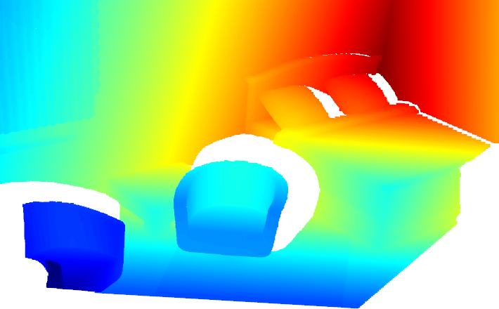
(b) Ground-truth (point cloud)

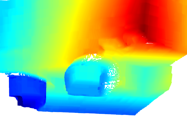
(c) BPG

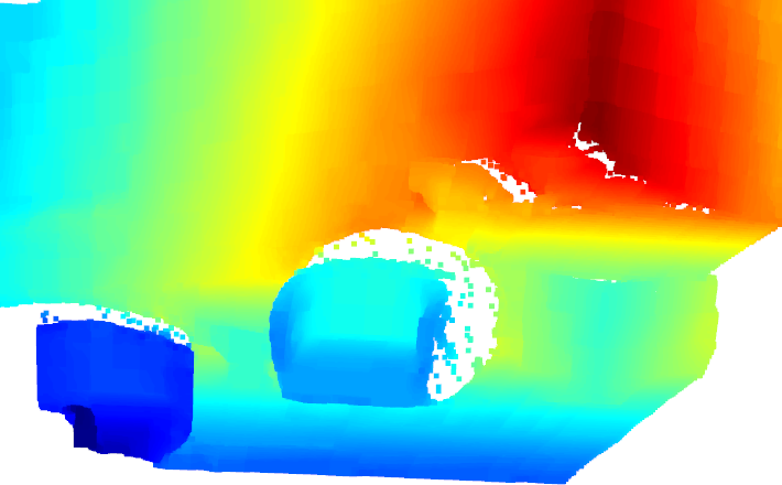
(d) $X_{\alpha}$ with $\alpha=0$ (equivalent to $G_{p}$)

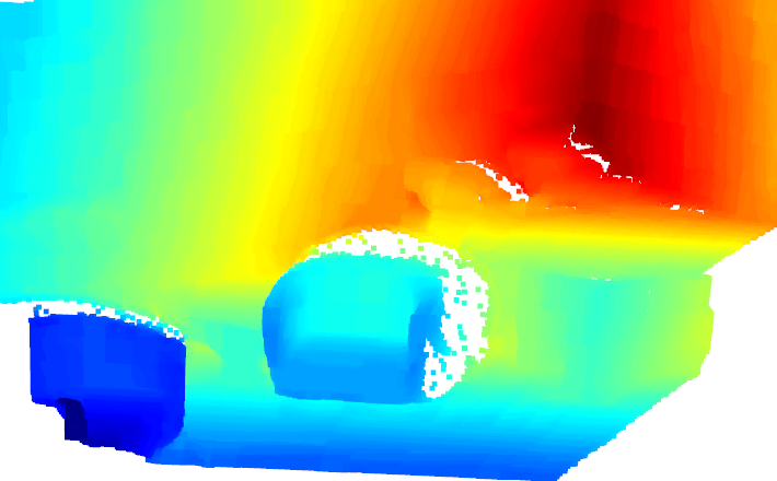
(e) $X_{\alpha}$ with $\alpha=0.25$

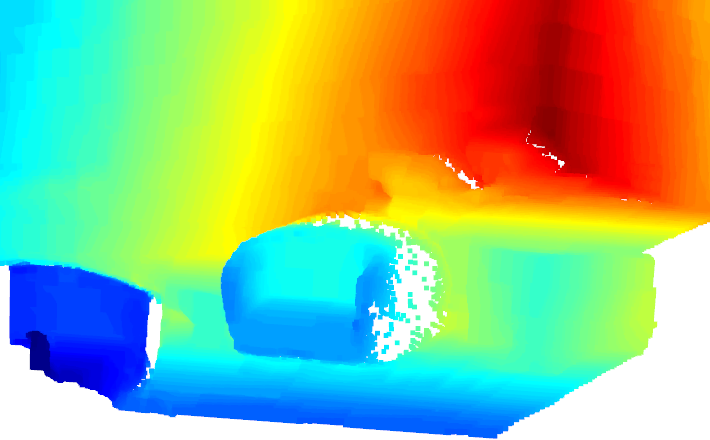
(f) $X_{\alpha}$ with $\alpha=0.5$

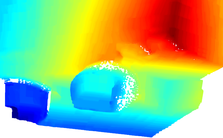
(g) $X_{\alpha}$ with $\alpha=0.75$

Figure 6: An illustration of applying Framework B to Post-process the BPG Codec on the SUNCG dataset. (a) Ground-truth depth image. (b) Point cloud corresponding to (a). (c) Point cloud reconstructed from the output of BPG. (d)-(g) Interpolation results. For visual clarity, the point cloud results are provided instead of depth image results.

Section 5.2 has provided results on depth images by training a post-processing perceptual decoding network (i.e., the proposed Framework B as shown in Figure 1(b)) to learn the distribution of the source conditioned on the MMSE decoding. From Theorem 2, Framework B is optimal if ($E_{d}$,$G_{d}$) is an MMSE encoder-decoder pair, which is a strict condition in practice. However, this framework applies to any existing compression system that optimized only in terms of distortion (may be not optimized in terms of MSE). In fact, there exist many traditional lossy compression systems that do not consider perceptual decoding but only optimized to minimize certain distortion measures.

Here, we apply Framework B to post-process the BPG codec. We provide experimental results on depth images, in which the encoder-decoder pair $(E_{d},G_{d})$ in Framework B is replaced by BPG codec. BPG (QP=40) is used to replace $(E_{d},G_{d})$ in Figure 1(b), and we train a post-processing network $G_{p}$ to improve the perceptual quality of the BPG output. The parameters are set the same as in Section 5.2.

Figure 6 shows the results on a typical sample from the SUNCG dataset. For visual clarity, the point cloud results are provided instead of depth image results. Although BPG is not optimal in MSE, our framework still shows high effectiveness by post perceptual decoding. The outputs of $G_{p}$ is much closer to the ground-truth than that of BPG.

Appendix D Result on RGB Images

Here, we provide more samples for qualitative comparison on RGB images. The image samples are from in KODAK dataset, as shown in Figure 7-Figure 9. The state-of-the-art method HiFiC is compared. Compared with the MMSE decoder $G_{d}$, the outputs of both Framework A and Framework B contain more details and the edges are sharper.

Besides, we also study the effect of $\lambda$ in (12) on the practical performance of the proposed Framework A. Theoretically, by Theorem 2, for any $\lambda<1$, optimizing (12) leads to perfect perception decoding. However, as explained in Remark 5, the discriminator in WGAN-gp is not strictly 1-Lipschitz and the capacity of the used network is not infinite. Hence, in practice the optimal solution cannot be achieved, especially when data distribution is complex, e.g., RGB images. We test different values of $\lambda$ when training the proposed Framework A. The quantitative results on the KODAK dataset are provided in Table LABEL:lambdatable, including the PSNR and three perception indices. It can be seen that, as the value of $\lambda$ decreases, the PSNR decreases but each perception index improves.

Figure 10 presents the decoding outputs of the proposed Framework A with different $\lambda$ on a typical sample. As shown in Figure 10, when $\lambda\geq 0.2$, the visual quality of the decoding outputs is similar to that of the MMSE decoding. When $\lambda\leq 0.1$, the visual quality improves significantly as more conspicuous details can be observed, but artifacts also increase.

Since the tuning of adversarial training is much involved, we believe that the perceptual quality of the proposed frameworks can be further improved by more intensive tuning of the hyper-parameters and network architecture.

(a) Ground-truth

(b) $G_{d}$ (MMSE)

(c) HiFiC

(d) Framework A ($\alpha=0$ and $\alpha=0.5$)

(e) Framework B ($\alpha=0$ and $\alpha=0.5$)

Figure 7: Example-1: Decoding outputs of the compared methods on a sample form the KODAK dataset.

(a) Ground-truth

(b) $G_{d}$ (MMSE)

(c) HiFiC

(d) Framework A ($\alpha=0$ and $\alpha=0.5$)

(e) Framework B ($\alpha=0$ and $\alpha=0.5$)

Figure 8: Example-2: Decoding outputs of the compared methods on a sample form the KODAK dataset.

(a) Ground-truth

(b) $G_{d}$ (MMSE)

(c) HiFiC

(d) Framework A ($\alpha=0$ and $\alpha=0.5$)

(e) Framework B ($\alpha=0$ and $\alpha=0.5$)

Figure 9: Example-3: Decoding outputs of the compared methods on a sample form the KODAK dataset.

Table 2: RGB image decoding results by the proposed Framework A for different values of $\lambda$ in (12) (on the KODAK dataset).

$\lambda$	PSNR	PI	Ma	NIQE
MMSE	38.36	4.54	6.36	5.45
0.4	38.27	3.93	6.82	4.68
0.2	37.73	3.09	7.68	3.78
0.1	37.22	2.45	8.26	3.16
0.05	37.18	2.12	8.60	2.84
0.01	36.89	2.05	8.74	2.84
0.005	36.96	1.98	8.75	2.71

(a) Ground-truth

(b) MMSE

(c) $\lambda=0.4$

(d) $\lambda$=0.2

(e) $\lambda$=0.1

(f) $\lambda$=0.05

(g) $\lambda$=0.01

(h) $\lambda$=0.005

Figure 10: Decoding outputs of the proposed Framework A with different $\lambda$ on a typical sample from the KODAK dataset.

References

- Agustsson et al. (2017) Agustsson, E., Mentzer, F., Tschannen, M., Cavigelli, L., Timofte, R., Benini, L., and Gool, L. V. Soft-to-hard vector quantization for end-to-end learning compressible representations. In Proceedings of the Conference on Neural Information Processing Systems (NeurIPS), pp. 1141–1151, 2017.
- Agustsson et al. (2019) Agustsson, E., Tschannen, M., Mentzer, F., Timofte, R., and Van Gool, L. Generative adversarial networks for extreme learned image compression. In Proceedings of the IEEE International Conference on Computer Vision (ICCV), pp. 221–231, 2019.
- Blau & Michaeli (2018) Blau, Y. and Michaeli, T. The perception-distortion tradeoff. In Proceedings of the IEEE Conference on Computer Vision and Pattern Recognition (CVPR), pp. 6228–6237, 2018.
- Blau & Michaeli (2019) Blau, Y. and Michaeli, T. Rethinking lossy compression: The rate-distortion-perception tradeoff. In Proceedings of the International Conference on Machine Learning (ICML), pp. 675–685, 2019.
- Blau et al. (2018) Blau, Y., Mechrez, R., Timofte, R., Michaeli, T., and Zelnik-Manor, L. The 2018 PIRM challenge on perceptual image super-resolution. In Computer Vision - ECCV 2018 Workshops - Munich, Germany, September 8-14, 2018, Proceedings, Part V, volume 11133, pp. 334–355, 2018.
- Chen & Koltun (2017) Chen, Q. and Koltun, V. Photographic image synthesis with cascaded refinement networks. In Proceedings of the IEEE International Conference on Computer Vision (ICCV), pp. 1520–1529, 2017.
- Cover & Thomas (2006) Cover, T. M. and Thomas, J. A. Elements of Information Theory. John Wiley and Sons, 2nd edition, 2006.
- Dosovitskiy & Brox (2016) Dosovitskiy, A. and Brox, T. Generating images with perceptual similarity metrics based on deep networks. In Proceedings of the Conference on Neural Information Processing Systems (NeurIPS), pp. 658–666, 2016.
- Freirich et al. (2021) Freirich, D., Michaeli, T., and Meir, R. A theory of the distortion-perception tradeoff in wasserstein space. In Proceedings of the Conference on Neural Information Processing Systems (NeurIPS), 2021.
- Galteri et al. (2017) Galteri, L., Seidenari, L., Bertini, M., and Bimbo, A. D. Deep generative adversarial compression artifact removal. In Proceedings of the IEEE International Conference on Computer Vision (ICCV), pp. 4836–4845, 2017.
- Gatys et al. (2016) Gatys, L. A., Ecker, A. S., and Bethge, M. Image style transfer using convolutional neural networks. In Proceedings of the IEEE Conference on Computer Vision and Pattern Recognition (CVPR), pp. 2414–2423, 2016.
- Goodfellow et al. (2014) Goodfellow, I. J., Pouget-Abadie, J., Mirza, M., Xu, B., Warde-Farley, D., Ozair, S., Courville, A., and Bengio, Y. Generative adversarial nets. In Proceedings of the Conference on Neural Information Processing Systems (NeurIPS), pp. 2672–2680, 2014.
- Guo et al. (2021) Guo, Z., Zhang, Z., Feng, R., and Chen, Z. Soft then hard: Rethinking the quantization in neural image compression. In Meila, M. and Zhang, T. (eds.), Proceedings of the International Conference on Machine Learning (ICML), volume 139, pp. 3920–3929. PMLR, 2021.
- Ishaan et al. (2017) Ishaan, G., Faruk, A., Martin, A., Vincent, D., and Courville, A. C. Improved training of wasserstein gans. In Proceedings of the Conference on Neural Information Processing Systems (NeurIPS), pp. 5767–5777, 2017.
- Iwai et al. (2020) Iwai, S., Miyazaki, T., Sugaya, Y., and Omachi, S. Fidelity-controllable extreme image compression with generative adversarial networks. In 25th International Conference on Pattern Recognition, ICPR 2020, pp. 8235–8242. IEEE, 2020.
- Johnson et al. (2016) Johnson, J., Alahi, A., and Fei-Fei, L. Perceptual losses for real-time style transfer and super-resolution. In Proceedings of the European Conference on Computer Vision (ECCV), pp. 694–711, 2016.
- Lecun et al. (1998) Lecun, Y., Bottou, L., Bengio, Y., and Haffner, P. Gradient-based learning applied to document recognition. Proceedings of the IEEE, 86(11):2278–2324, 1998.
- Ledig et al. (2017) Ledig, C., Theis, L., Huszár, F., Caballero, J., Cunningham, A., Acosta, A., Aitken, A., Tejani, A., Totz, J., Wang, Z., and Shi, W. Photo-realistic single image super-resolution using a generative adversarial network. In Proceedings of the IEEE Conference on Computer Vision and Pattern Recognition (CVPR), pp. 105–114, 2017.
- Li et al. (2018) Li, M., Zuo, W., Gu, S., Zhao, D., and Zhang, D. Learning convolutional networks for content-weighted image compression. In Proceedings of the IEEE Conference on Computer Vision and Pattern Recognition (CVPR), pp. 3214–3223, 2018.
- Lin et al. (2014) Lin, T., Maire, M., Belongie, S. J., Hays, J., Perona, P., Ramanan, D., Dollár, P., and Zitnick, C. L. Microsoft COCO: common objects in context. In Computer Vision - ECCV 2014 - 13th European Conference, Zurich, Switzerland, September 6-12, 2014, Proceedings, Part V, volume 8693, pp. 740–755. Springer, 2014.
- M Tschannen (2018) M Tschannen, E Agustsson, M. L. Deep generative models for distribution-preserving lossy compression. In Proceedings of the Conference on Neural Information Processing Systems (NeurIPS), pp. 5933–5944, 2018.
- Ma et al. (2017) Ma, C., Yang, C., Yang, X., and Yang, M. Learning a no-reference quality metric for single-image super-resolution. Comput. Vis. Image Underst., 158:1–16, 2017.
- Matsumoto (2018) Matsumoto, R. Introducing the perception-distortion tradeoff into the rate-distortion theory of general information sources. IEICE Communications Express, 7(11):427–431, 2018.
- Matsumoto (2019) Matsumoto, R. Rate-distortion-perception tradeoff of variable-length source coding for general information sources. IEICE Communications Express, 2019.
- Mentzer et al. (2018) Mentzer, F., Agustsson, E., Tschannen, M., Timofte, R., and Gool, L. V. Conditional probability models for deep image compression. In Proceedings of the IEEE Conference on Computer Vision and Pattern Recognition (CVPR), pp. 4394–4402, 2018.
- Mentzer et al. (2020) Mentzer, F., Toderici, G., Tschannen, M., and Agustsson, E. High-fidelity generative image compression. In Proceedings of the Conference on Neural Information Processing Systems (NeurIPS), 2020.
- Minnen et al. (2018) Minnen, D., Ballé, J., and Toderici, G. Joint autoregressive and hierarchical priors for learned image compression. In Bengio, S., Wallach, H. M., Larochelle, H., Grauman, K., Cesa-Bianchi, N., and Garnett, R. (eds.), Proceedings of the Conference on Neural Information Processing Systems (NeurIPS), pp. 10794–10803, 2018.
- Mirza & Osindero (2014) Mirza, M. and Osindero, S. Conditional generative adversarial nets. CoRR, abs/1411.1784, 2014.
- Mittal et al. (2013a) Mittal, A., Soundararajan, R., and Bovik, A. C. Making a completely blind image quality analyzer. IEEE Signal Process. Lett., 20(3):209–212, 2013a.
- Mittal et al. (2013b) Mittal, A., Soundararajan, R., and Bovik, A. C. Making a ”completely blind” image quality analyzer. IEEE Signal Process. Lett., 20(3):209–212, 2013b.
- Ohayon et al. (2021) Ohayon, G., Adrai, T., Vaksman, G., Elad, M., and Milanfar, P. High perceptual quality image denoising with a posterior sampling CGAN. In IEEE/CVF International Conference on Computer Vision Workshops, ICCVW 2021, Montreal, BC, Canada, October 11-17, 2021, pp. 1805–1813. IEEE, 2021.
- Prakash et al. (2021) Prakash, M., Delbracio, M., Milanfar, P., and Jug, F. Removing pixel noises and spatial artifacts with generative diversity denoising methods. CoRR, abs/2104.01374, 2021.
- Rippel & Bourdev (2017) Rippel, O. and Bourdev, L. Real-time adaptive image compression. In Proceedings of the International Conference on Machine Learning (ICML), pp. 2922–2930, 2017.
- Salimans et al. (2016) Salimans, T., Goodfellow, I. J., Zaremba, W., Cheung, V., Radford, A., and Chen, X. Improved techniques for training gans. In Proceedings of the Conference on Neural Information Processing Systems (NeurIPS), pp. 2226–2234, 2016.
- Santurkar et al. (2018) Santurkar, S., Budden, D. M., and Shavit, N. Generative compression. In Proceedings of the Picture Coding Symposium (PCS), pp. 258–262, 2018.
- Shannon (1959) Shannon, C. Coding theorems for a discrete source with a fidelity criteria. IRE Nat. Conv. Rec., 4, 01 1959.
- Simonyan & Zisserman (2015) Simonyan, K. and Zisserman, A. Very deep convolutional networks for large-scale image recognition. In Proceedings of the International Conference on Learning Representations (ICLR), 2015.
- Song et al. (2017) Song, S., Yu, F., Zeng, A., Chang, A. X., Savva, M., and Funkhouser, T. A. Semantic scene completion from a single depth image. In 2017 IEEE Conference on Computer Vision and Pattern Recognition, CVPR 2017, Honolulu, HI, USA, July 21-26, 2017, pp. 190–198. IEEE Computer Society, 2017.
- Toderici et al. (2016) Toderici, G., O’Malley, S. M., Hwang, S. J., Vincent, D., Minnen, D., Baluja, S., Covell, M., and Sukthankar, R. Variable rate image compression with recurrent neural networks. In Proceedings of the International Conference on Learning Representations (ICLR), 2016.
- Toderici et al. (2017) Toderici, G., Vincent, D., Johnston, N., Hwang, S. J., Minnen, D., Shor, J., and Covell, M. Full resolution image compression with recurrent neural networks. In Proceedings of the IEEE Conference on Computer Vision and Pattern Recognition (CVPR), pp. 5435–5443, 2017.
- Wang et al. (2022) Wang, W., Wen, F., Yan, Z., and Liu, P. Optimal transport for unsupervised denoising learning. IEEE Transactions on Pattern Analysis and Machine Intelligence, 2022.
- Wang et al. (2018) Wang, X., Yu, K., Wu, S., Gu, J., Liu, Y., Dong, C., Qiao, Y., and Loy, C. C. ESRGAN: Enhanced super-resolution generative adversarial networks. In Proceedings of the European Conference on Computer Vision Workshops (ECCVW), pp. 63–79, 2018.
- Wang & Simoncelli (2005) Wang, Z. and Simoncelli, E. P. Reduced-reference image quality assessment using a wavelet-domain natural image statistic model. In Rogowitz, B. E., Pappas, T. N., and Daly, S. J. (eds.), Human Vision and Electronic Imaging X, volume 5666, pp. 149–159, 2005.
- Wang et al. (2003) Wang, Z., Simoncelli, E. P., and Bovik, A. C. Multiscale structural similarity for image quality assessment. In The Thrity-Seventh Asilomar Conference on Signals, Systems Computers, 2003.
- Wu et al. (2020) Wu, L., Huang, K., and Shen, H. A gan-based tunable image compression system. In Proceedings of the IEEE Winter Conference on Applications of Computer Vision (WACV), pp. 2323–2331, 2020.
- Yan et al. (2021) Yan, Z., Wen, F., Ying, R., Ma, C., and Liu, P. On perceptual lossy compression: The cost of perceptual reconstruction and an optimal training framework. In Proceedings of the International Conference on Machine Learning (ICML), volume 139, pp. 11682–11692, 2021.
- Zhang et al. (2021) Zhang, G., Qian, J., Chen, J., and Khisti, A. Universal rate-distortion-perception representations for lossy compression. volume abs/2106.10311, 2021.
- Zhang et al. (2016) Zhang, R., Isola, P., and Efros, A. A. Colorful image colorization. In Proceedings of the European Conference on Computer Vision (ECCV), 2016.
- Zhang et al. (2018) Zhang, R., Isola, P., Efros, A. A., Shechtman, E., and Wang, O. The unreasonable effectiveness of deep features as a perceptual metric. In Proceedings of the IEEE Conference on Computer Vision and Pattern Recognition (CVPR), pp. 586–595, 2018.
- Zhang et al. (2018) Zhang, Y., Li, K., Li, K., Wang, L., Zhong, B., and Fu, Y. Image super-resolution using very deep residual channel attention networks. In Computer Vision - ECCV 2018 - 15th European Conference, Munich, Germany, September 8-14, 2018, Proceedings, Part VII, volume 11211, pp. 294–310. Springer, 2018.
- Zhou Wang et al. (2004) Zhou Wang, Bovik, A. C., Sheikh, H. R., and Simoncelli, E. P. Image quality assessment: from error visibility to structural similarity. IEEE Transactions on Image Processing, 13(4):600–612, 2004.