Event-Case Correlation for Process Mining using Probabilistic Optimization

Abstract

Process mining supports the analysis of the actual behavior and performance of business processes using event logs. An essential requirement is that every event in the log must be associated with a unique case identifier (e.g., the order ID of an order-to-cash process). In reality, however, this case identifier may not always be present, especially when logs are acquired from different systems or extracted from non-process-aware information systems. In such settings, the event log needs to be pre-processed by grouping events into cases – an operation known as event correlation. Existing techniques for correlating events have worked with assumptions to make the problem tractable: some assume the generative processes to be acyclic, while others require heuristic information or user input. Moreover, they abstract the log to activities and timestamps, and miss the opportunity to use data attributes. In this paper, we lift these assumptions and propose a new technique called EC-SA-Data based on probabilistic optimization. The technique takes as inputs a sequence of timestamped events (the log without case IDs), a process model describing the underlying business process, and constraints over the event attributes. Our approach returns an event log in which every event is associated with a case identifier. The technique allows users to incorporate rules on process knowledge and data constraints flexibly. The approach minimizes the misalignment between the generated log and the input process model, maximizes the support of the given data constraints over the correlated log, and the variance between activity durations across cases. Our experiments with various real-life datasets show the advantages of our approach over the state of the art.

1 Introduction

Recent years have seen a drastically increasing availability of process execution data from various data sources [1, 2, 3]. Process mining offers different analysis techniques that can extract business insights from these data, known as event logs. Each event in a log must have at least three attributes [4, 5]: (i) the event class referring to a specific activity in the process (e.g., “Order checked” or “Claim assessed”), (ii) the end timestamp capturing the occurrence of the event, and (iii) the case identifier (e.g., the order number in an order-to-cash process, or the claim ID in a claims handling process). Recent process mining algorithms such as $\alpha\$$ [6], Inductive Miner [7], Evolutionary Tree Miner [8], Fodina [9], Structured Heuristic Miner [10], Split Miner [11], and the Hybrid ILP Miner [12] need all of these three attributes together for discovering a process model.

Various data infrastructures such as data lakes often give more attention to data storage than to structuring them such that process mining can be readily applied [13, 14]. Prior research has described the problem of missing case identifiers as a correlation problem, because the connections between different events have to be reestablished based on heuristics, domain knowledge or payload data. In essence, the correlation problem is concerned with identifying which events belong to the same case when a unique case identifier is missing. This identification can be done by an event correlation engine (see Figure 1). An event correlation engine constructs a correlated log with case identifiers by using domain knowledge, e.g. about the process control flow, organizational resources, maximal task durations, or other data knowledge over the event attributes. Existing correlation techniques face the challenge of operating in a large search space. For this reason, previous proposals have introduced assumptions to make the problem tractable. The main assumptions they have in common is abstracting a log on activities and timestamps with ignoring the other attributes. Moreover, some techniques assume the generative processes to be acyclic [15, 16] while others require heuristic information about the execution behavior of activities in addition to the process model [17]. Beyond that, these approaches suffer from poor efficiency and miss the opportunity to make use of data attributes.

In previous work [18], we introduced a probabilistic optimization technique called EC-SA (Events Correlation by Simulated Annealing), which is based on a simulated annealing heuristic approach. EC-SA addresses the correlation problem as a multi-level optimization problem. In this paper, we extend EC-SA to consider a broader spectrum domain knowledge for the correlation process, integrating ideas of mixing process specification paradigms [19]. We call the extension EC-SA-Data. Using the domain knowledge about the event data attributes improves the event correlation process as it decreases the random assigning of events to their corresponding cases. The technique revolves around three nested objectives. First, it seeks to minimize the misalignment between the generated log and an input process model. Second, it aims to maximize the support of the given data constraints over the correlated log. Third, it targets to minimize the activity execution time variance across cases. The latter objective builds on the assumption that the same activities tend to have similar duration across cases. Our extensive evaluation demonstrates the benefits of our novel technique.

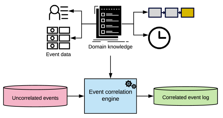
Figure 1: Overview of the event correlation engine

The remainder of this paper is organized as follows. Section 2 discusses prior research on the event correlation problem. Section 3 defines preliminaries that are essential for our technique. Section 4 presents the different phases of our novel EC-SA-Data event correlation technique. Section 6 then discusses the experimental evaluation on real-life logs before Section 7 concludes the paper.

2 Related Work

The correlation problem focuses on identifying two or more variables that are related, even though this relationship is not explicitly define. It received adequate attention in the data science research field for static data [20, 21, 22]. The existing techniques have various objectives to improve the analysis, monitoring and mining of the data. Database correlation techniques work on improving query performance of knowledge discovery. Jermaine [23] discusses the discovery of correlations between database attributes. He develops measures of independence between the attributes to discover the actual correlation, and analyses the computational complexity of correlation techniques. Brown and Haas [24] present a data-driven technique that discovers the hidden relation between database attributes and integrates them into an optimizer to improve query performance. Though valuable for data, these works cannot be directly applied for process mining event correlation. They lack a notion of temporal order.

In this paper, we focus on a specific instance of the event correlation problem: how to correlate those events that have been generated from the execution of the same process instance? An event correlation technique takes as input at least an uncorrelated log [25]. Depending on whether or not a technique relies on additional input, we classify existing techniques into four categories: 1) requiring no additional input; 2) requiring a process model; 3) relying on correlation conditions; and 4) relying on event similarity functions.

The first category of techniques uses as input only event names and ignores the other event data attributes. Ferreira and Gillbald [16] provide an Expectation-Maximization (E-Max) approach that builds a Markov model from the uncorrelated log and discovers the possible process behavior in the uncorrelated log. This technique is adversely sensitive to the density of the working cases within the system,i.e., the number of overlapping cases at a given point in time. Also, it does not support concurrency and cyclic process behaviors. Walicki and Ferreira [26] provide a sequence partitioning approach that searches for the minimal set of patterns that can represent the process behavior in an uncorrelated log. The technique does not support concurrency and cyclic process behaviors.

The second category includes correlation techniques that use timestamps of events and the process model. The Correlation Miner (CMiner) by Pourmiza et al. [27] builds on two matrices, one capturing proceed/succeed relations and another one capturing the time difference between pairs of events. An optimal correlation is calculated using integer linear programming. An extension of the CMiner [15] uses quadratic programming to find the optimal correlation by minimizing the duration between the events. CMiner does not support cyclic processes and relies on quadratic constraints solving, which limits its scalability. Experiments reported in [15] show that the approach can only handle logs with a few dozen cases. The Deducing Case Ids (DCI) approach [28] requires a process model and heuristic information about the activity execution durations. The approach utilizes a breadth-first approach to build a case decision tree to explore the solution space. In [17], DCI is extended with a pre-processing step to detect the cyclic behavior and build a relationship matrix for the correlation decision. DCI supports cyclic processes. It is sensitive to the quality of the input data, such that if the model and the log have low fitness, then the generated correlated logs will contain noise and missing events. Also, it is computationally inefficient due to the breadth-first search approach. In a previous paper [18], we propose the Event Correlation by Simulated Annealing (EC-SA) approach, which uses the event names and timestamp in addition to the process model. EC-SA addresses the correlation problem as a multi-level optimization problem, as it searches for the nearest optimal correlated log considering the fitness with an input process model and the activities’ timed behavior within the log. The accuracy of the given model affects the quality of the correlated log, and the performance is affected by the number of uncorrelated events.

The third category includes correlation techniques that use event data attributes and apply correlation conditions to correlate the events. Motahari-Nezhad et al. [29] propose a semi-automated correlation approach to correlate the web service messages based on the correlation conditions. The approach derives correlation conditions using the event data from different data layers. Also, it computes the interestingness of the attributes of the events to prune the conditions search space. Thus, it generates several log partitions and possible process views. The approach requires user-defined domain parameters and intermediate domain expert feedback to guide the correlation process. Engel et ¨[30] propose the EDImine framework, which allows for the usage of process mining over electronic data interchange (EDI) messages. EDIminer resorts to message flow mining and physical activity mining methods to generate the events from EDI messages. Then, EDIminer employs user-defined correlation rules to correlate the events to their cases. This framework is limited to EDI messages and depends on the user-defined parameters for the event generation and the correlation process. Reguieg et al. [31] propose a MapReduce-based approach to derive the correlation conditions from the service interaction logs. It consists of two stages. The first stage defines the simple correlation conditions. The second stage derives more complex correlation conditions and correlates the events to their cases. In [32], the authors extend their previous work to improve scalability and efficiency. They introduce two strategies to perform the log partition and explore the complex correlation condition space. The main challenges of the approach are the log partitioning and the vast amount of network traffic communication. Cheng et al. [33] propose the Rule Filtering and Graph Partitioning (RF-Grap) approach, which follows the filtering and verification principle to improve the efficiency of event correlation using distributed platforms. RF-Grap prunes a large number of uninteresting correlation rules in the filtering step. Accordingly, not all the derived rules are investigated, but only the interesting rules that fulfil the criteria. In the verification steps, they use graph partitioning to decompose the correlation possibilities over the clusters. De Murillas et al. [34] propose an approach to extract the event log from a database based on the redo logs that contain the events of data manipulation. They use a data model to define the relation between the events. In [35], the authors provide a way to automatically generate different event logs from a database by defining the case notion based on the data relations in the data model. A case notion defines which events should be considered for the correlation based on the selected data objects that represent the investigated cases. They measure the interestingness of the generated logs and recommend the highest one to the user.

The fourth category includes the correlation techniques that rely on event similarity or the case identifier in the log. Djedović et al. [36] propose an algorithm to compute the similarity between pairs of events to correlate events with higher similarity. Event similarity function defined over the equality between the attributes over the events. The optimal correlation represents the highest similarity score between the case’s events. The approach expects the existence of main attributes that do not change over the case. Abbad Andaloussi et al. [37] address the correlation problem under the assumption that event data already contains the case identifier. For each event log attribute A, the technique discovers a process model assuming that A is the case identifier. The resulting models are compared based on four quality measures. The attribute that yields the highest-quality model is taken as the case identifier. Bala et al. [13] follow a similar direction based on the idea that identifiers are repetitive in the log. Burattin and Vigo [38] propose a framework that generalized from a real business case. They search the activities attributes over the log to define the possible process instance attributes. Then they used the equality relation between these attributes to correlate the events to their cases. This method relies on a-prior knowledge about the application domain and user-defined heuristic parameters, such as the number of events within a case and characteristics of the candidate attributes.

In summary, the approaches in the first category assume that the process is acyclic. Those in the second category expect that a full process model is available. The third category require correlation rules to be provided or discovered heuristically. Approaches in the fourth category assume that there is a case identifier attribute or a similarity function that allows to group events. The technique presented in this paper extends EC-SA approach. It integrates the strengths of the first and second category. Unlike the first category, it can handle cyclic behavior. It also allows users to provide additional domain knowledge that will support the correlation process. In this way, it relaxes the dependence on the control-flow knowledge.

3 Preliminaries

In this section, we discuss the fundamental notions that our approach builds upon. Section 3.1 describes the data structures we handle. Section 3.2 outlines our process modeling and execution language and notations. Section 3.3 illustrates the fundamental mechanisms underpinning simulated annealing, a core technique for our solution .

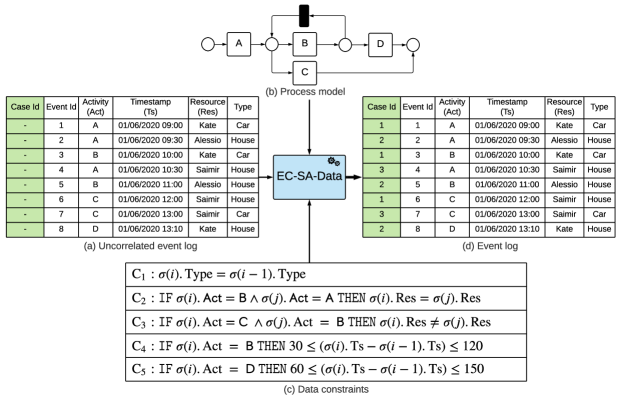
Figure 2: Running example of a sample loan application check process

3.1 Process Event Data Structures

Starting with the basic notion of event (i.e., the atomic unit of execution), we introduce the uncorrelated event log, case and projection of a case over an event attribute. Thereupon, we present the definitions of event log and trace.

Definition 1 (Event)

Let $E\ni e$ be a finite non-empty set of symbols. We refer to $e$ as event and to $E$ as the universe of events.

Definition 2 (Attribute)

Given a non-empty set of domain values $\textrm{Dom}\in\mathfrak{D}$, an attribute $\textrm{Attr}\in\mathfrak{A}$ is a partial function $\textrm{Attr}:E\nrightarrow\textrm{Dom}$ mapping events to domain values. We indicate the value mapped by Attr to an event $e$ by using a dot notation, i.e., $e.\textrm{Attr}$.

In the following, we assume without loss of generality that attributes $\mathrm{Act}$ and $\mathrm{Ts}$ are total functions defined over events. The range of the former is a finite subset of strings we interpret as activity names and the range of the latter is a finite subset of integers to be interpreted as timestamps. For example, $e_{1}$ in Fig. 2 is mapped to four different values, one per attribute: $e_{1}.\mathrm{Act}=\mathsf{A}$ represents the executed activity, $e_{1}.\mathrm{Ts}=$“$\mathsf{07/06/2020\ 09:00}$” represents the completion timestamp, $e_{1}.\mathrm{Res}=\mathsf{R}1$ represents the operating resource, and $e_{1}.\mathrm{Type}=\mathsf{Home}$ represents additional data knowledge about the event context.

Definition 3 (Uncorrelated log)

Let $E\ni e$ be the universe of events, $\mathfrak{D}\ni\textrm{Dom}$ the universe of domain values and $\mathfrak{A}\ni\textrm{Attr}$ a set of attributes defined over $E$ as per Def.s 1 and 2. Given a total order defined over $E$, $\preccurlyeq\;\subseteq E\times E$ (henceforth referred to as event ordering), the uncorrelated log is a tuple $\mathrm{UL}=(E,\mathfrak{D},\mathfrak{A},\preccurlyeq)$.

We assume the mapping of $\mathrm{Ts}$ to be coherent with $\preccurlyeq$, i.e., if $e\preccurlyeq e^{\prime}$ then $e.\mathrm{Ts}\leqslant e^{\prime}.\mathrm{Ts}$. Considering the total ordering as a mapping from a convex subset of integers, we can assign to every event a unique integer index (or event id for short), induced by $\preccurlyeq$ on the events. We shall denote the index $i\in[1,|E|]$ of an event $e$ as a subscript, $e_{i}$. For example, Fig. 2(a) depicts an uncorrelated log and $e_{3}$ is its third event.

Definition 4 (Event log)

Let $\mathrm{UL}=(E,\mathfrak{D},\mathfrak{A},\preccurlyeq)$ be an uncorrelated log as per Def. 3 and $I\ni\iota$ be a universe of case identifiers (or case id’s for short). An event log is a triple $L=(\mathrm{UL},I,\ell)$ where $\ell:E\to I$ is a total surjective function.

Notice that $\ell$ induces a partition of $E$ into $|I|$ subsets. Figure 2(d) illustrates an event log. Notice that $I=\{1,2,3\}$ and $\ell$ maps events $e_{1}$, $e_{3}$ and $e_{6}$ to $1$, $e_{2}$, $e_{5}$ and $e_{8}$ to $2$, and $e_{4}$ and $e_{7}$ to $3$. We name the sequences of events that stem from mapping $\ell$ and preserve $\preccurlyeq$ as cases.

Definition 5 (Case)

Given a case id $\iota\in I$ and an event log $L$ as per Def. 4, a case $\sigma$ defined by $\iota$ over $L$ is a finite sequence $\langle e_{\sigma,1},\ldots,e_{\sigma,n}\rangle\in E^{*}$ of length $|\sigma|=n\in\mathbb{N}$ of events $e_{\sigma,i}\textrm{ with }1\leqslant i\leqslant n$ such that (i) $\ell(e_{\sigma,i})=\iota$ and (ii) the sequence is induced by $\preccurlyeq$, i.e., $e_{\sigma,j}\preccurlyeq e_{\sigma,i}$ for every $j$ s.t. $j\leqslant i\leqslant n$.

For example, the event log depicted in Fig. 2(d) is comprised of $3$ cases. Case $\sigma_{1}$ defined by case id $1$ is $\langle e_{1},e_{3},e_{6}\rangle$. Notice that it preserves the order of the events within the case. We name the projection of a case over the activities of its events as trace.

Definition 6 (Trace)

Given a case $\sigma=\langle e_{\sigma,1},\ldots,e_{\sigma,n}\rangle\in E^{*}$ and the total attribute function $\mathrm{Act}:E\to\mathrm{Dom}_{\mathrm{Act}}$, a trace $t\in\mathrm{Dom}_{\mathrm{Act}}^{*}$ is the sequence induced by case $\sigma$ through the mapping of $\mathrm{Act}$, i.e., $t=\langle e_{\sigma,1}.\mathrm{Act},\ldots,e_{\sigma,n}.\mathrm{Act}\rangle$.

In our example, the trace corresponding to $\sigma_{1}$ is $\langle\mathsf{A},\mathsf{B},\mathsf{C}\rangle$.

Short-hand notations

For the sake of readability, we shall use the following short-hand notations:

$L(\iota)$

indicates the case defined by $\iota$ over $L$; in the example of Fig. 2(d), e.g., $L(2)=\langle e_{2},e_{5},e_{8}\rangle$;

$S(L)$

denotes the set of all cases defined over event log $L$, i.e., $S(L)=\{L(\iota)|\iota\in I\}$; it follows that $|I|=|S(L)|$; in our example, $S(L)=\{\sigma_{1},\sigma_{2},\sigma_{3}\}$ where $\sigma_{1}=\langle e_{1},e_{3},e_{6}\rangle$, $\sigma_{2}=\langle e_{2},e_{5},e_{8}\rangle$, $\sigma_{3}=\langle e_{4},e_{7}\rangle$;

$\sigma(i)$

refers to the $i$-th event within a case $\sigma$ (e.g., the first event in $\sigma_{1}$ is denoted as ${\sigma_{1}(1)}$, whereby $\sigma_{1}(1)=e_{1}$ in our example);

$\sigma[i,j]$

indicates the segment of case $\sigma$ from $i$ to $j$, having $1\leqslant i\leqslant j\leqslant|\sigma|$ (e.g., $\sigma_{1}[2,3]=\langle e_{3},e_{6}\rangle$ );

$\mathrm{Act}(\sigma)$

denotes with a slight abuse of notation the trace induced by case $\sigma$ trough the mapping of $\mathrm{Act}$ (e.g., $\mathrm{Act}(\sigma_{1})=\langle\mathsf{A},\mathsf{B},\mathsf{C}\rangle$);

$e\in\sigma$

indicates that there exists an index $i$, $1\leqslant i\leqslant n$ such that $\sigma(i)=e$ (e.g., $e_{5}\in\sigma_{2}$);

$\langle e,e^{\prime},e^{\prime\prime},\ldots,e^{(m)}\rangle\subseteq\sigma$

indicates that there exists an index $j$ with $1\leqslant j\leqslant n-m$ such that $\sigma(j)=e,\sigma(j+1)=e^{\prime},\sigma(j+2)=e^{\prime\prime},\ldots,\sigma(j+m)=e^{(m)}$, where $n$ is the length of $\sigma$ and $m\leq n$ (e.g., $\langle e_{2},e_{5}\rangle\subseteq\sigma_{2}$);

$\sigma=\sigma^{\prime}$

holds if and only if $\sigma\subseteq\sigma^{\prime}$ and $\sigma^{\prime}\subseteq\sigma$.

3.2 Process Modeling and Execution

In this section we outline the main notions we shall adopt in the remainder of this paper about process modeling and execution.

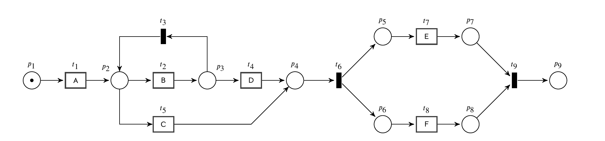
Figure 3: A workflow net

Alongside uncorrelated event logs and data constraints, our approach takes as input a behavioral model for processes. We require that the process model has a starting activity and an accepting state. In the context of this paper, we resort to workflow nets [39] such as the one in Fig. 3. Workflow nets are bipartite graphs consisting of (i) a finite non-empty set of nodes partitioned into places (graphically depicted as circles – e.g., $\{p_{1},\ldots,p_{9}\}$ in Fig. 3) and transitions (rectangles – e.g., $\{t_{1},\ldots,t_{9}\}$), and (ii) a flow relation, namely arcs connecting places to transitions and transitions to places (e.g., $p_{1}\to t_{1}$, $t_{1}\to p_{2}$ and $t_{5}\to p_{2}$); the set of places at the tail of flow arcs toward a transition are the preset of that transition (e.g., the presets of $t_{2}$ and $t_{9}$ are $\{p_{2}\}$ and $\{p_{7},p_{8}\}$, respectively); places at the head of flow arcs are the postset of the transition (e.g., the postsets of $t_{2}$ and $t_{6}$ are $\{p_{3}\}$ and $\{p_{5},p_{6}\}$, respectively).

Transitions can be annotated with an activity name (e.g., $t_{1}$ is annotated with $\mathsf{A}$); otherwise, they are silent (in which case, they are graphically depicted as a solid black rectangle as with $t_{5}$, $t_{6}$ and $t_{9}$ in the figure). The set of places contain exactly one input and one output place, namely a source and a sink node for the graph, respectively – e.g., $p_{1}$ and $p_{9}$. Every node in the workflow net is reachable through a directed walk from the input place.

The execution semantics are specified by the production and consumption of tokens (represented as black dots). A transition can be executed (i.e., it is enabled) only if a token is in every place of its preset. The execution implies that a token is consumed from every place in its preset and a token is produced in every place in its postset. In the beginning, a token resides in the input place ($p_{1}$ in the figure) by default – therefore, it is sometimes omitted from the graphical representation. Transition $t_{1}$, in the example, is the only one enabled at the beginning. Its execution consumes the token from $p_{1}$ and produces a token in $p_{2}$. Then, both $t_{2}$ and $t_{3}$ are enabled. Notice that their execution is thus mutually exclusive and that $t_{3}$ enacts a cyclic behavior. Executing $t_{2}$ and then $t_{4}$ enables $t_{6}$ which, in turn, can consume a token from $p_{4}$ and produce two tokens (one in $p_{5}$ and the other in $p_{6}$), thereby enabling both $t_{7}$ and $t_{8}$. Notice that $t_{9}$ is enabled only if a token is assigned to $p_{7}$ and another one to $p_{8}$. Therefore, $t_{7}$ and $t_{8}$ have to be executed, regardless of the order. The execution of $t_{9}$ consumes a token from $p_{7}$ and a token from $p_{8}$ to ultimately produce one in $p_{9}$, the output place. The sequence of executions of enabled transitions from the initial state (with a token in the input place) to the final one (with a token in the output place) is a run of the Workflow net. The physical time it take for a run to complete, from start to end, is called cycle time.

As previously discussed, a trace is a sequence of activities. The transcription of activities decorating the sequentially executed transitions determines a trace too. Notice that the execution of silent transitions such as $t_{5}$ in the example does not occur in a trace. Traces that correspond to runs of the Workflow net in Fig. 3 are, e.g., $\langle\mathsf{A},\mathsf{C},\mathsf{E},\mathsf{F}\rangle$, $\langle\mathsf{A},\mathsf{B},\mathsf{B},\mathsf{D},\mathsf{E},\mathsf{F}\rangle$ and $\langle\mathsf{A},\mathsf{B},\mathsf{D},\mathsf{F},\mathsf{E}\rangle$.

Traces can be replayed to check if they correspond to a run of a Workflow net. If an activity in the sequence cannot be bound to the execution of an enabled transition, or requires one or more (non-silent) transitions to be previously executed though they are not recorded in the trace, we say an asynchronous move occurs. The computation of those alignments [40] is at the basis of a well-known technique for conformance checking [41]. For example, $\langle\mathsf{A},\mathsf{B},\mathsf{B},\mathsf{B},\mathsf{D},\mathsf{F},\mathsf{E}\rangle$ conforms with the process model in Fig. 3, thus the alignment consists of sole synchronous moves. Instead, $\langle\mathsf{A},\mathsf{B},\mathsf{C},\mathsf{E},\mathsf{F}\rangle$ does not conform with it as $\mathsf{B}$ is a move in the log that cannot correspond to a move in the model. Similarly, $\langle\mathsf{A},\mathsf{E},\mathsf{F}\rangle$ requires the execution of transition $\mathsf{C}$ before the occurrence of $\mathsf{E}$ although it is not recorded in the trace. Intuitively, the fewer asynchronous moves occur, the higher the fitness of model and log is. The computation of alignments and quality measures for process mining are beyond the scope of this paper. The interested reader can find a detailed examination of these topics in [41].

3.3 Simulated Annealing

We address the correlation problem as an optimization problem and, to solve it, we resort to simulated annealing. Simulated Annealing (SA) is a metaheuristic algorithm that explores the optimization problem’s search space to find the nearest approximate global solution by simulating the cooling process of metals through the annealing process [42, 43]. SA applies the stochastic perturbation theory [44] to search for an approximate global solution by randomly changing the next individuals in order to skip the iterations’ local optimal solution[45].

A population-based SA [46] allows for the use of multiple individuals in the same iteration of the annealing process. SA explores the search space through the following steps. It starts by creating the initial population. A population ($\mathrm{pop}$) is a non-empty set of individuals ($|\mathrm{pop}|\geq 1$). The population is formed by generating random individuals. Then the SA algorithm initializes the current step $S_{\mathrm{curr}}$ as $S_{\mathrm{curr}}=1$ and the current temperature with a given initial temperature, $\uptau_{\mathrm{curr}}=\uptau_{\mathrm{init}}$. The annealing process begins with the generation of a neighbor solution $x^{\prime}$ for the current individual $x$. Therefore, SA considers as a memory-less algorithm because it disregards the historical individuals, and only focuses on $x$ and $x^{\prime}$. Next, SA computes the energy cost function based on $x$ and $x^{\prime}$, namely $\delta\mathrm{f_{c}}(x,x^{\prime})$.

The acceptance probability of the new neighbor solution $\mathrm{prob}(x^{\prime})$ is computed using $\delta\mathrm{f_{c}}(x,x^{\prime})$ and $\uptau_{\mathrm{curr}}$. In particular, $\mathrm{prob}(x^{\prime})$ determines whether the new neighbor, $x^{\prime}$, can be used as the next individual. Notice that $\mathrm{prob}(x^{\prime})$ may select $x^{\prime}$ even though it performs worse than $x$ in order to increase the chances to skip the local optimum and let the algorithm explore the search space further, especially with high temperatures. At each iteration, SA compares the global optimal solution $x_{\mathrm{G}}$, i.e., the best solution over the iterations $[0,S_{\mathrm{curr}}[$, with the local optimal solution $x_{\mathrm{L}}$ in $\mathrm{pop}$ at $S_{\mathrm{curr}}$ based on $\delta\mathrm{f_{c}}(x_{\mathrm{G}},x_{\mathrm{L}})$. Therefore, SA can return the best solution over all the iterations. Finally, SA uses a cooling schedule [47] that defines the rate at which the temperature ($\uptau_{\mathrm{curr}}$) cools down, and increments $S_{\mathrm{curr}}$ by $1$. SA repeats the annealing and cooling process until $S_{\mathrm{curr}}$ reaches the maximum number of iterations ($S_{\mathrm{max}}$).

To sum up, SA has a set of parameters that influence the annealing process: (i) the initial temperature ($\uptau_{\mathrm{init}}$), (ii) the maximum number of steps ($S_{\mathrm{max}}$), and (iii) the population size ($|\mathrm{pop}|$). In addition to these parameters, SA requires the following main functions to be defined: (i) the cooling schedule, (ii) the creation of a new neighbor ($x^{\prime}$), (iii) the energy cost function ($\delta\mathrm{f_{c}}(x,x^{\prime})$), and (iv) the acceptance probability ($\mathrm{prob}(x^{\prime})$).

4 The EC-SA-Data Solution

Equipped with the definitions and main notions defined in the above section, we define the input (I1, I2, I3), preconditions (P1, P2), output (O1) and effects (E1) of EC-SA-Data.

I1.

An uncorrelated log $\mathrm{UL}$, as per Def. 3 (depicted, e.g., in Fig. 2(a)).

I2.

A process model (e.g., the Workflow net depicted in Fig. 2(b)).

P1.

The process model is required to have exactly one start activity (e.g., $\mathsf{A}$ in Fig. 2(b)), which is enabled only at the beginning of the run, and thus cannot be part of any cycle.

P2.

The process model is required to have a final state (such a state, e.g., is reached after $\mathsf{C}$ or $\mathsf{D}$ are executed with the model in Fig. 2(b)).

I3.

A set of domain knowledge rules, i.e., data constraints on process data $\mathfrak{C}=\{C_{1},\dots,C_{m}\}$. In the following, we will interchangeably use the terms “rule” and “data constraint”. Constraints are propositions [48] exerted on resources, time or additional event attributes. Syntax and semantics of the constraint expression language will be described in Section 4.3. Figure 2(c), e.g., illustrates four such constraints.

O1.

EC-SA-Data generates an event log $L$ as per Def. 4.

E1.

The event log partitions $\mathrm{UL}$ into a set of cases, i.e., for every event $e\in\mathrm{UL}$ there exists one and only one case $\sigma\in L$ s.t. $e\in\sigma$ (see, e.g., Fig. 2(d)).

The key idea of the EC-SA-Data technique is to treat the event correlation problem as a multi-level optimization problem. EC-SA-Data has three nested objectives: (i) minimizing the misalignment between the generated event log and the input process model, (ii) minimizing the constraints violations over the cases, and (iii) minimizing the activity execution time variance across the cases.

EC-SA-Data uses multi-level simulated annealing (SA) as an optimization technique [46]. Using SA to solve the event correlation problem helps to find an approximate global optimal correlated log in a reasonable time. To apply SA to solve the event correlation problem, we define the functions required by the SA:

1. The cooling schedule $\uptau_{\mathrm{curr}}$;

2. The creation of a new neighbor ($x^{\prime}$);

3. The energy cost function ($\delta\mathrm{f_{c}}(x,x^{\prime})$);

4. The acceptance probability ($\mathrm{prob}(x^{\prime})$).

Figure 4 shows the steps of EC-SA-Data. We describe them in detail in the following subsections.

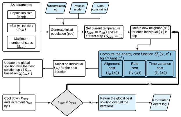
Figure 4: The EC-SA-Data technique overview

4.1 Initial population

As shown in Fig. 4, the first step is the generation of the initial population, $\mathrm{pop}$, of size $|\mathrm{pop}|\geq 1$. An individual $x\in\mathrm{pop}$ is a candidate event log as defined as per Def. 4. For the sake of readability, we graphically depict the individuals as graphs such as that of Fig. 6. In the following, we shall name these graphs as log graphs, or LG’s for short.

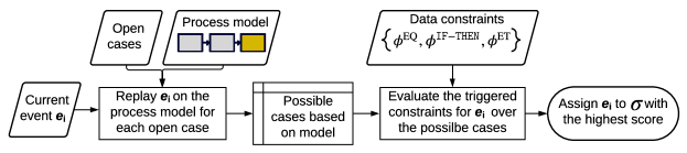
Figure 5: Event correlation decision process for event $e_{i}$

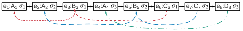
Figure 6: Log graph $LG_{1}$ of individual $x$

As shown in Fig. 6, every node in the log graph represents an event within the uncorrelated log, its assigned case and the related activity. For example, the third node represents $e_{3}$, assigned with case $\sigma_{1}$ and annotated with $\mathsf{B}_{3}$ as its activity $e_{3}$.$\mathrm{Act}$ is $\mathsf{B}$. We keep the event index as a subscript to distinguish the position in which activities recur in the log (e.g., $\mathsf{B}_{3}$ and $\mathsf{B}_{5}$ denote the occurrence of activity $\mathsf{B}$ with events $e_{3}$ and $e_{5}$). The log graph depicts two different flow connections. The first flow is represented via forward solid arcs connecting every event to its direct successor according to the temporal order in the uncorrelated log. The second flow connection (depicted with backward dashed arcs) connects every event to its direct predecessor in the same case. For example, backward dashed arcs connect $e_{7}$ to $e_{5}$ and $e_{5}$ to $e_{2}$ in the figure as these events belong to case $\sigma_{2}=\langle e_{2},e_{5},e_{7}\rangle$.

The data structure underlying the log graph is generated by replaying the uncorrelated event log on the process model and verifying the data constraints over the possible case assignments. This step is repeated based on the population size. In our example, we assume $|\mathrm{pop}|=1$ for readability purposes.

Figure 5 shows the steps taken to correlate an event $e_{i}$. The first step filters out the possible candidate cases for $e_{i}$ based on the process model replay. Then, we rank the candidate cases based on the number of data constraints thereby satisfied by $e_{i}$ in those cases. These steps are repeated for every event in $\mathrm{UL}$.

4.2 Process model based correlation

Every run of the process model from the initial activity to the termination conditions corresponds to a case. We name the cases corresponding to non-terminated runs as open cases. We figure the following three scenarios when replaying an event $e$ over the input process model.

1. Event $e$ corresponds to the execution of the start activity of the process model (we name it start event). Then, a new run starts and a new case is open, accordingly.

2. Event $e$ corresponds to the execution of an enabled (non-starting) activity for one or more cases (enabled event). If only one run enables $e$, it is assigned to the case of that run. Otherwise, $e$ is assigned to the case satisfying the highest number of data constraints.

3. Event $e$ does not correspond to any enabled activity (non-enabled event). Then, $e$ is assigned to the case satisfying the highest number of data constraints. This way, we guarantee that all events are correlated, even if the log deviates from the model.

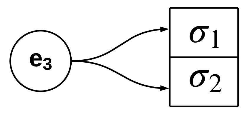
(a) Possible cases for $e_{3}$

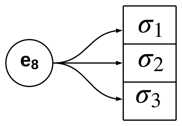
(b) Possible cases for $e_{8}$

Figure 7: Process model based assignment of cases for events $e_{3}$ and $e_{8}$

For example, considering $\mathrm{UL}$ in Fig. 2(a) and the process model in Fig. 2(b), $e_{1}$ is a start event as it executes the start activity ($\mathsf{A}$). Thus, it opens a new case, $\sigma_{1}$. The same goes for $e_{2}$ and $e_{4}$, which start $\sigma_{2}$ and $\sigma_{3}$, respectively. There are two open cases within the log before $e_{3}$: both $\sigma_{1}$ and $\sigma_{2}$ expect the execution of activity $\mathsf{B}$ or activity $\mathsf{C}$. Therefore, $e_{3}$ is an enabled event and both cases are considered as possible candidate assignments for the data-constraint based correlation step, as shown in Fig. 7(a). On the other hand, based on the assigned cases in Fig. 6, none of the cases $\sigma_{1}$, $\sigma_{2}$ and $\sigma_{3}$ expect the execution of activity $\mathsf{D}$. Thus, $e_{8}$ is a non-enabled event and all the three cases are considered for data constraints based correlation step in order to reduce the randomization of the correlation decision, as shown in Fig. 7(b). Following Fig. 5, we identify the possible case-assignments of an event based on the model that will be used in the next step.

4.3 Data constraint based correlation

Knowledge about data attributes provides an additional source of information for correlation. Intuitively, we use data constraints to filter and rank the cases to which an event can be assigned. In the context of this paper, we focus on the following types of data constraints. To define them, we take inspiration from the work of Nehzad et al. [29, 15] and extend it with IF-THEN rules. Though not intended to constitute an exhaustive set, we focus on these templates as we experimentally found them to be a good trade-off between expressiveness and tractability. Further studies on the suitability and effectiveness of the data constraints in use are beyond the scope of this work and subject to future research.

Definition 7 (Equality constraint)

Let $\sigma(i)$ and $\sigma(i-1)$ be two consecutive events in a case $\sigma$ as per Def. 5. A data-attribute equality constraint (henceforth equality constraint for short) $\phi^{\textrm{EQ}}$ is a predicate over variables $\sigma(i)$ and $\sigma(i-1)$ formulated as follows:

$$\phi^{\textrm{EQ}} \coloneqq\sigma(i).\mathrm{Attr}\>=\>\sigma(i-1).\mathrm{Attr}$$

For example, ${C_{1}}$ in Fig. 2 (i.e., $\sigma(i).\mathrm{Type}\leavevmode\nobreak\ =\leavevmode\nobreak\ \sigma(i-1).\mathrm{Type}$) enforces the equality between the $\mathrm{Type}$ attribute values. As depicted in Fig. 7(a), $e_{3}$ reports the execution of activity $\mathsf{B}$. One of the possible cases, based on the process model, is $\sigma_{1}$. The constraint is evaluated over $\sigma(i)=e_{3}$ and $\sigma(i-1)=e_{1}$.

Definition 8 (IF-THEN constraint)

Let $\sigma(i)$ be an event in a case $\sigma$ as per Def. 5 and $j$ an index $1\leq j<i$; let $E$ be a universe of events and Attr an attribute $\textrm{Attr}:E\nrightarrow\textrm{Dom}$ as per Def. 2. An IF-THEN constraint $\phi^{\texttt{IF}\textrm{-}\texttt{THEN}}$ is a predicate over pairs of events consisting of two propositional clauses: the antecedent (the IF clause) and consequent (the THEN close). We define the syntax of well-formed IF-THEN constraints as follows.

$$\phi^{\texttt{IF}\textrm{-}\texttt{THEN}} \coloneqq\mathtt{\texttt{IF}}\>\varphi_{\texttt{IF}}^{i}\>{\texttt{THEN}}\>\varphi_{\texttt{THEN}}^{i,j}\wedge j=i-1$$

$$\>\>\>\>\>\>\>|\>{\texttt{IF}}\>\varphi_{\texttt{IF}}^{i,j}\>{\texttt{THEN}}\>\varphi_{\texttt{THEN}}^{i,j}\wedge j<i$$

$$\varphi_{\texttt{IF}}^{i} \coloneqq\sigma(i)\mathtt{.}\textrm{Attr}\lessgtr a\>|\>\varphi_{\texttt{IF}}^{i}\>\wedge\>\sigma(i)\mathtt{.}\textrm{Attr}\lessgtr a$$

$$\varphi_{\texttt{IF}}^{i,j} \coloneqq\varphi_{\texttt{IF}}^{i}\>\wedge\>\sigma(j)\mathtt{.}\textrm{Attr}\lessgtr a\>$$

$$\>\>\>\>\>\>\>|\>\varphi_{\texttt{IF}}^{i,j}\>\wedge\>\sigma(j)\mathtt{.}\textrm{Attr}\lessgtr a$$

$$\varphi_{\texttt{THEN}}^{i,j} \coloneqq\widehat{\varphi}_{\texttt{THEN}}^{i,j}\>|\>\varphi_{\texttt{THEN}}^{i,j}\mathrel{\begin{subarray}{c}\vee\\ \wedge\end{subarray}}\widehat{\varphi}_{\texttt{THEN}}^{i,j}$$

$$\widehat{\varphi}_{\texttt{THEN}}^{i,j} \coloneqq\sigma(j)\mathtt{.}\textrm{Attr}\lessgtr a\>|\>\sigma(i)\mathtt{.}\textrm{Attr}\lessgtr\sigma(j)\mathtt{.}\textrm{Attr}^{\prime}$$

$$\lessgtr \coloneqq<\>|\>>\>|\>\geq\>|\>\leq\>|\>=\>|\>\neq$$

$$\mathrel{\begin{subarray}{c}\vee\\ \wedge\end{subarray}} \coloneqq\vee\>|\>\wedge$$

In the following, we may collectively refer to $\varphi_{\texttt{IF}}^{i}$ and $\varphi_{\texttt{IF}}^{i,j}$ as $\varphi_{\texttt{IF}}$, and to $\varphi_{\texttt{THEN}}^{i}$ and $\varphi_{\texttt{THEN}}^{i,j}$ as $\varphi_{\texttt{THEN}}$ for the sake of readability.

$\phi^{\texttt{IF}\textrm{-}\texttt{THEN}}$ is an association rule in which $\varphi_{\texttt{IF}}$ and $\varphi_{\texttt{THEN}}$ act as selection and verification criteria, respectively. In other words, $\varphi_{\texttt{IF}}$ seeks a pair of events, i.e., an event $\sigma(i)$ and a preceding event $\sigma(j)$, that satisfy the IF clause. EC-SA-Data gives priority to the closest $j$ to $i$ in the selection process. Notice that if $\varphi_{\texttt{IF}}$ is in the $\varphi_{\texttt{IF}}^{i}$ form, we impose $j=i-1$ by default (see the grammar rule above). Subsequently, $\varphi_{\texttt{THEN}}$ is evaluated on the selected events to check whether $\sigma(i)$ and $\sigma(j)$ satisfy $\phi^{\texttt{IF}\textrm{-}\texttt{THEN}}$. For instance, the evaluation of $C_{2}$ in Fig. 2 (i.e., IF $\sigma(i).{\mathsf{Act}}=\mathsf{B}$ and $\sigma(j).{\mathsf{Act}}={\mathsf{A}}$ THEN $\sigma(i).{\mathrm{Res}}=\sigma(j).\mathrm{Res}$) selects two events based on their activities ($\sigma(i).{\mathsf{Act}}=\mathsf{B}$ and $\sigma(j).{\mathsf{Act}}={\mathsf{A}}$) and then checks whether the resources are equal for those events ($\sigma(i).{\mathrm{Res}}=\sigma(j).\mathrm{Res}$). In the example above, let us take $e_{3}$. We notice that $e_{3}.\mathrm{Act}$ is $\mathsf{B}$ and one of the assignable cases (based on the process model) is $\sigma_{1}$ as illustrated in Fig. 7(a). Considering the log graph illustrated in Fig. 6, we pick $\sigma(2)=e_{3}$ and select $\sigma(1)=e_{1}$ as $e_{1}.\mathrm{Act}=\mathsf{A}$. Then, the THEN clause is evaluated over the two events: $(e_{3}.\mathrm{Res}=e_{1}.\mathrm{Res})\equiv\mathrm{True}$. We conclude that $C_{2}$ is satisfied by $e_{3}$ and $e_{1}$ in case $\sigma_{1}$.

Definition 9 (Event-time constraint)

Let $\sigma(i)$ and $\sigma(i-1)$ be two consecutive events in a case $\sigma$ as per Def. 5. An event-time constraint $\phi^{\textrm{ET}}$ is a predicate over $\sigma(i)$ and $\sigma(i-1)$ consisting of two propositional clauses: an antecedent (IF clause) that selects $\sigma(i)$ and a consequent (THEN clause) that bounds the event execution duration $(\sigma(i).\mathrm{Ts}-\sigma(i-1).\mathrm{Ts})$ to a given minimum duration (dur) and a given maximum duration (dur’) as follows.

$$\phi^{\textrm{ET}} \coloneqq\texttt{IF}\>\varphi_{\texttt{IF}}^{i}\>\texttt{THEN}\>\varphi_{\texttt{THEN}}^{\textrm{ET}}$$

$$\varphi_{\texttt{THEN}}^{\textrm{ET}} \coloneqq\textrm{dur}\leq\left(\sigma(i).\mathrm{Ts}-\sigma(i-1).\mathrm{Ts}\right)\leq\textrm{dur}^{\prime}$$

$\phi^{\textrm{ET}}$ is based upon the grammar of IF-THEN constraints to express rules on the activity execution duration. In particular, the IF clause selects $\sigma(i)$ based on propositional formulas, while $\sigma(j)$ is the directly preceding event $\sigma(i-1)$, taken in order to compute the event duration $(\sigma(i).\mathrm{Ts}-\sigma(i-1).\mathrm{Ts})$.

For example, $C_{4}$ in Fig. 2 (i.e., ${\texttt{IF}\leavevmode\nobreak\ }\sigma(i).\mathrm{Act}=\mathsf{B}{\leavevmode\nobreak\ \texttt{THEN}\leavevmode\nobreak\ }$ $30\leq(\sigma(i).\mathrm{Ts}-\sigma(i-1).\mathrm{Ts})\leq 120$) requires that the duration of activity $\mathsf{B}$ is between $30\text{\,}\mathrm{min}$ and $120\text{\,}\mathrm{min}$. $e_{3}$ reports the execution of activity $\mathsf{B}$. One of the assignable cases as per the process model is $\sigma_{1}$, as illustrated in Fig. 7(a). Considering the log graph illustrated in Fig. 6, we select $\sigma(i)=e_{3}$ and compute the duration based on $\sigma(i-1)=e_{1}$, which amounts to $60\text{\,}\min$. Thus, the THEN clause holds true as $30\leq 60\leq 120$.

We collectively refer to equality, IF-THEN and event-time constraints as data constraints.

Definition 10 (Data constraint)

Let $L$ be an event log defined over events in $E\ni e$ and let $\sigma\in S(L)$ be a case as per Def.s 4 and 5. A data constraint $C$ is a predicate $\phi$ over events that belongs to either of the following three types: data-attribute equality constraint (as per Def. 7, hitherto indicated with the expression “$C\textrm{ is }\phi^{\textrm{EQ}}$”), IF-THEN constraint (as per Def. 8, “$C\textrm{ is }\phi^{\texttt{IF}\textrm{-}\texttt{THEN}}$”), or event-time constraint (Def. 9, “$C\textrm{ is }\phi^{\textrm{ET}}$”). The set of all possible constraints over $E$ is the universe of data constraints $\mathfrak{C}\ni C$.

EC-SA-Data employs data constraints to rank possible case assignments based on the number of satisfied ones. To pursue our objective, we first need to restrict the evaluation of constraints to a current event under analysis. Therefore, we introduce the notion of $i$-preassignment: rather than seeking pairs of events at position $i$ and $j<i$ in a case $\sigma$ that satisfy a constraint, we fix $i$ to an event $e\in\sigma$ so as to be able to check whether any $j$ exists such that the constraint is satisfied by $\sigma(i)$ and $\sigma(j)$ in $\sigma$.

Definition 11 ($i$-Preassignment)

Let $L$ be an event log over the universe of events $E\ni e$ and $S(L)\ni\sigma$ be its case set as per Def.s 1, 4 and 5. Let $C\in\mathfrak{C}$ be a data constraint expressed by formula $\phi$ as per Def. 10. Denoting with $\overrightarrow{\imath}(\sigma,e)$ the index of $e$ in case $\sigma$, the $i$-preassignment of $\phi$ with $e$ is the assignment of $\sigma(i)$ with $e$ in its formula, i.e., $\phi[i/\,\overrightarrow{\imath}(\sigma,e)]$.

The $i$-Preassignment predetermines the $i$-th event to be considered for the evaluation of the constraint. In the case of IF-THEN and event-time rules, this entails that only $j$, with $1\leqslant j<i\leqslant|\sigma|$, is sought for in order to have $C$ satisfied by $\sigma(i)$ and $\sigma(j)$. For example, consider case $\sigma_{1}$ as illustrated in Fig. 2(d) and constraint $C_{2}={\texttt{IF}}\leavevmode\nobreak\ \sigma(i).{\mathrm{Act}}={\mathsf{B}}\wedge\sigma(j).{\mathrm{Act}}={\mathsf{A}}\leavevmode\nobreak\ {\texttt{THEN}}\leavevmode\nobreak\ \sigma(i).\mathrm{Res}=\sigma(j).{\mathrm{Res}}$ (Fig. 2(c)). With a slight abuse of notation, we extend the notion of $i$-preassignment to clauses within the formulation of a constraint (e.g., $\varphi_{\texttt{IF}}[i/\,\overrightarrow{\imath}(\sigma,e)]$). For example, although the IF clause of $C_{2}$ would be satisfied in $\sigma_{1}$ by setting $i=2$ and $j=1$ (i.e., considering $e_{3}$ and $e_{1}$), but it would not be satisfied if $i$-preassigned with $e_{6}$ as $e_{6}.\mathrm{Act}=\mathsf{C}$.

Equipped with this notion, we define how to check if an $i$-preassigned constraint is satisfied in a case. Notice we consider IF-THEN and event-time constraints as satisfied if and only if both the IF and THEN clauses are satisfied, unlike the common interpretation of an “if-then” implication may suggest. This design choice is motivated by the goal to avoid that the ex falso quod libet statement applies (i.e., that in case the antecedent evaluates to false, the constraint holds true regardless of the consequent), as it reportedly leads to an overestimation of the support of a given rule, as explained in detail in the context of declarative process mining [49, 50, 51]. Considering the example above, $C_{2}$ $i$-preassigned with $e_{6}$ is not satisfied because its IF clause is not satisfied either.

The score function, formalized in the following, counts the number of satisfied constraints that are $i$-preassigned with an event.

Definition 12 (Score function)

Let $E$ be the universe of events as per Def. 1, $S(L)$ represent the cases of log $L$ as per Def. 5 and $\mathfrak{C}$ be the universe of constraints as per Def. 10. Considering the $i$-preassignment with $e$ $\phi[i/\,\overrightarrow{\imath}(\sigma,e)]$ as per Def. 11, let $\mathrm{eSat}:\mathfrak{C}\times E\times S(L)\to\{0,1\}$ be a function that indicates whether an $i$-preassigned constraint is satisfied given $e\in E$ in case $\sigma\in S(L)$ as follows:

Let $\mathscr{C}\subseteq\mathfrak{C}$ be a set of constraints. The score function $\mathrm{score}:2^{\mathfrak{C}}\times E\times S(L)\to\mathbb{N}$ counts the satisfied constraints within a set $\mathscr{C}\in\mathfrak{C}$ given event $e\in E$ in case $\sigma\in S(L)$ as follows:

$$\mathrm{score}(\mathscr{C},e,\sigma)=\sum_{C\in\mathscr{C}}{\mathrm{eSat}(C,e,\sigma)}$$ (2)

We use the data constraints to guide the selection of the most proper case for an event $e$. We identify the best candidate as the first one ranked by the score. If multiple cases share the highest score, we randomly select one of them. Randomness is legitimate in this context as it helps to escape the local optimal solution over subsequent SA-iterations.

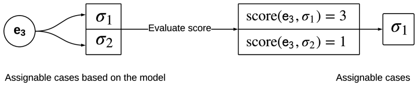
(a) Correlation decision for $e_{3}$

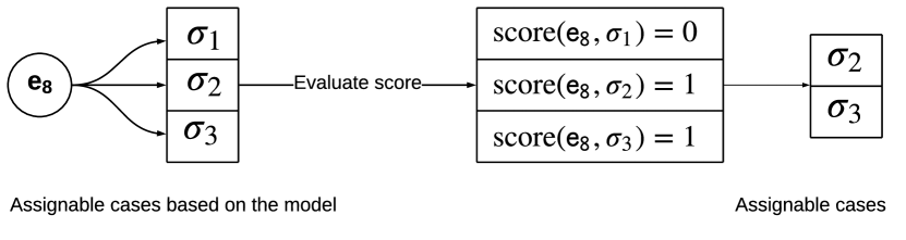
(b) Correlation decision for $e_{8}$

Figure 8: Event correlation decision for events $e_{3}$ and $e_{8}$

For example, considering the process model in Fig. 2(b) and the data constraints in Fig. 2(c), EC-SA-Data generates the individual represented as log graph $\mathrm{LG}_{1}$ in Fig. 11(a) from the uncorrelated log in Fig. 2(a). Scanning the events, we initially correlate $e_{1}$ with $\sigma_{1}$, and upon $e_{2}$, $\sigma_{2}$ starts. At this stage, there are two open cases before $e_{3}$: both $\sigma_{1}$ and $\sigma_{2}$ expect the occurrence of activity $\mathsf{B}$ or activity $\mathsf{C}$ because both are enabled as per the process model. Therefore, $e_{3}$ can belong to each of those cases, as shown in Fig. 8(a). Considering the data constraints in Fig. 2(c), let us focus on $C_{1}$, $C_{2}$ and $C_{4}$ in particular. They pertain to $e_{3}$ as $C_{1}$ verifies the equality of the $\mathrm{Type}$ attribute of an event with that of the preceding one (for all events), while $C_{2}$ and $C_{4}$ check that $\sigma(i).\mathrm{Act}=\mathsf{B}$ in their IF clause (and $e_{3}.\mathrm{Act}=\mathsf{B}$). As for $C_{1}$ (i.e., $\sigma(i).\mathrm{Type}=\sigma(i-1).\mathrm{Type}$) and its $i$-preassignment with $e_{3}$, we observe that it is satisfied in $\sigma_{1}$ as $e_{1}.\mathrm{Type}$ is $\mathsf{Home}$ like $e_{3}.\mathrm{Type}$. Instead, the $i$-preassiged constraint is violated in $\sigma_{2}$ as $e_{2}.\mathrm{Type}$ is $\mathsf{Car}$, unlike $e_{3}.\mathrm{Type}$. Constraint $C_{2}$ (i.e., ${\texttt{IF}}\leavevmode\nobreak\ \sigma(i).{\mathrm{Act}}={\mathsf{B}}\wedge\sigma(j).{\mathrm{Act}}={\mathsf{A}}\leavevmode\nobreak\ {\texttt{THEN}}\leavevmode\nobreak\ \sigma(i).\mathrm{Res}=\sigma(j).{\mathrm{Res}}$), once $i$-preassigned with $e_{3}$, is satisfied in $\sigma_{1}$ as the IF and THEN clauses evaluate to $\mathrm{true}$ and $e_{1}.{\mathrm{Res}}=e_{3}.{\mathrm{Res}}={\mathsf{Kate}}$. Again, it is violated in $\sigma_{2}$ because $e_{1}.{\mathrm{Res}}\neq e_{3}.{\mathrm{Res}}$. As far as $C_{4}$ (${\texttt{IF}\leavevmode\nobreak\ }\sigma(i).\mathrm{Act}={\mathsf{B}}{\leavevmode\nobreak\ \texttt{THEN}\leavevmode\nobreak\ }30\leq(\sigma(i).\mathrm{Ts}-\sigma(i-1).\mathrm{Ts})\leq 120$) and its $i$-preassignment with $e_{3}$ are concerned, the execution duration of activity $\mathsf{B}$ in $\sigma_{1}$ is $e_{3}.\mathrm{Ts}-e_{1}.\mathrm{Ts}=$60\text{\,}\mathrm{min}$$. Also, in $\sigma_{2}$ we have $e_{3}.\mathrm{Ts}-e_{2}.\mathrm{Ts}=$30\text{\,}\mathrm{min}$$. Therefore, the $i$-preassigned $C_{4}$ is satisfied both in $\sigma_{1}$ and $\sigma_{2}$.

Then, we compute the score as in Eq. 2 to rank the possible cases. As shown in Fig. 8(a), $\sigma_{1}$ gets the highest score as it supports the three constraints unlike $\sigma_{2}$. Therefore, $e_{3}$ is assigned with $\sigma_{1}$ as graphically depicted in Fig. 6. Following this procedure, we observe that also $e_{6}$ is assigned with the same case later on.

To guarantee that even all events are associated to a case, we consider all cases as assignable also to non-enabled events. Again, we rank the cases based on their score to decide the assignment. For instance, $e_{8}$ is a non-enabled event, because neither of the three running cases $\sigma_{1}$, $\sigma_{2}$ and $\sigma_{3}$ expects the execution of activity $\mathsf{D}$. Therefore, $e_{8}$ is assigned based on the data constraints. Considering the constraints in Fig. 2(c), we focus on the $i$-preassignment of $C_{1}$ and $C_{5}$ with $e_{8}$ and evaluate them over $\sigma_{1}$, $\sigma_{2}$ and $\sigma_{3}$. As shown in Fig. 8(b), $\sigma_{1}$ gets the lowest score, as both $C_{1}[i/\,\overrightarrow{\imath}(\sigma_{1},e_{8})]$ and $C_{5}[i/\,\overrightarrow{\imath}(\sigma_{1},e_{8})]$ are violated. In $\sigma_{2}$ and $\sigma_{3}$, instead, the $i$-preassigned $C_{1}$ is satisfied. Still, both $C_{5}[i/\,\overrightarrow{\imath}(\sigma_{2},e_{8})]$ and $C_{5}[i/\,\overrightarrow{\imath}(\sigma_{3},e_{8})]$ are violated as in both cases activity $\mathsf{D}$ exceeds the allowed maximum duration. Therefore, $e_{8}$ is randomly assigned with $\sigma_{3}$ as one of the cases with the highest score, as illustrated in Fig. 6.

4.4 Neighbor solution

As illustrated in Fig. 4, simulated annealing explores the search space by creating a new neighbor individual ($x^{\prime}$) based on the current individual ($x$) at the beginning of each iteration. We generate a neighbor ($x^{\prime}$) by altering the current individual ($x$). In particular, we modify the assignments of the events in the totally ordered set from a given point (henceforth named as changing point) on. In order to form a different solution, we reassign the events from the changing point till the end of the events in $\mathrm{UL}$ by following the event correlation decision steps in Fig. 5.

The current step ($S_{\mathrm{curr}}$) determines the extent wo which the new neighbor should differ. Thus, a changing point is selected based on the current step $S_{\mathrm{curr}}$. For instance, when $S_{\mathrm{curr}}=1$, the changing point is randomly selected among the first few events, to widely explore the space. Instead, when $S_{\mathrm{curr}}=S_{\mathrm{max}}-1$, the changing point is randomly picked among the last few events as we seek to converge toward a solution. The increment of $S_{\mathrm{curr}}$ reduces the number of events to be re-evaluated at each iteration; this is in line with the cooling down mechanism of the annealing process.

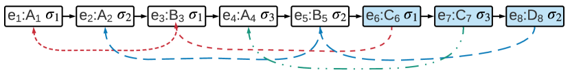
Figure 9: New individual $x^{\prime}$ based on $\mathrm{LG_{1}}$

For example, let $S_{\mathrm{max}}=2$ and $\uptau_{\mathrm{init}}=100$. After generating the initial individual in Fig. 6, we have $S_{\mathrm{curr}}=1$. Notice that, at this iteration, $S_{\mathrm{curr}}=S_{\mathrm{max}}-1$, so the changing point is randomly selected from the second half of the events in $\mathrm{UL}$, i.e., from $e_{5}$ to $e_{8}$. In this example, the changing point corresponds to $e_{6}$. As shown in Fig. 9, a new individual $x^{\prime}$ is thus created and we explore the possible assignments for events $e_{6}$, $e_{7}$ and $e_{8}$, while the other events are assigned as in $x$.

4.5 Energy cost function

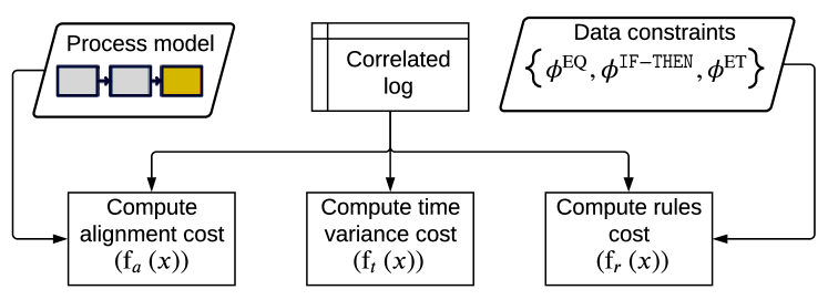
Figure 10: Energy cost functions

Simulated annealing uses the energy function to model the optimization problem. We model the event correlation problem as multi-level objectives optimization problem that has three level of objectives: (i) minimizing the misalignment between the generated event log and the input process model, (ii) minimizing the constraints violations over the cases, and (iii) minimizing the activity execution time variance across the cases.

We define an energy function for each of these objectives, as shown in Fig. 10. The first energy function ($\mathrm{f_{a}}(x)$) computes the cost of aligning $x$ and the model. The second energy function ($\mathrm{f_{r}}(x)$) computes the data rules violations cost within $x$. The third energy function ($\mathrm{f_{t}}(x)$) computes the activity execution time variance within $x$. They are used to compute the energy cost function between $x$ and $x^{\prime}$, $\delta\mathrm{f_{c}}(x,x^{\prime})$, as shown in Fig. 4. In the following, we elaborate on the individual energy functions and the computation of $\delta\mathrm{f_{c}}(x,x^{\prime})$.

4.5.1 Alignment cost

To measure the model-log misalignment we use the well-established alignment cost function proposed by Adriansyah et al. [52]. The technique penalizes every asynchronous move between the log and the model, that is to say, it associates a cost to every event that occurs in the trace although the model would not allow for it, or every missing event that the model would require to continue the run though the trace does not contain it.

Figure 11 shows an example of computing the log alignment cost $\mathrm{f_{a}}(x)$ over individual $x$ (depicted in Fig. 11(a)). The first step is to extract the cases from individual $x$ as shown in Fig. 11(d). Then, EC-SA-Data deduces the traces from the cases by projecting them over the cases’ activities as shown in Fig. 11(d). For each trace $\sigma$ in the log, it computes the alignment cost of the trace ($\Delta_{\textrm{algn}}(\mathrm{Act}(\sigma))$) with respect to the process model.

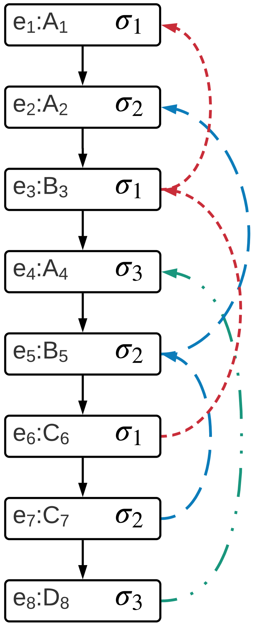
(a) Log graph of $x$

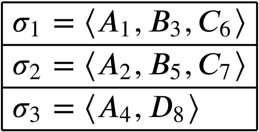
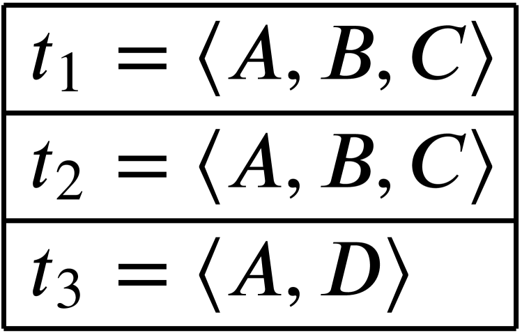
(b) Cases in $x$

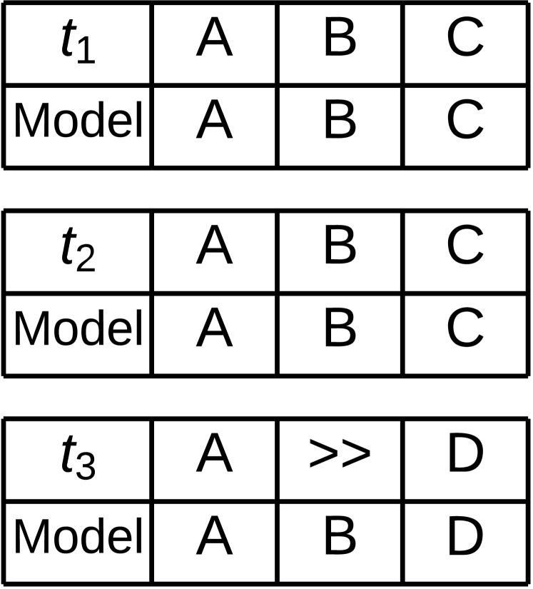
(c) Traces in $x$

(d) Alignments of traces in $x$

Figure 11: Computation of the alignments for individual $x$

The log alignment cost is finally computed as the summation of the trace alignment costs, as shown in Eq. 3.

$$\mathrm{f_{a}}(x)=\sum_{\sigma\in S(x)}{\Delta_{\textrm{algn}}(\mathrm{Act(\sigma)})}$$ (3)

For example, Fig. 11(d) shows that the execution of activity $\mathsf{D}$ in $t_{3}$ is considered as an asynchronous move as it is not enabled by the model (indicated with a guillemet in the figure, $\gg$). Thus, $\Delta_{\textrm{algn}}(t_{3})=1$. On the other hand, $\Delta_{\textrm{algn}}(t_{1})=\Delta_{\textrm{algn}}(t_{2})=0$ as $t_{1}$ and $t_{2}$ are in complete alignment with the model. The log alignment cost of $x$ (depicted in Fig. 11(a)) is $\mathrm{f_{a}}(x)=\Delta_{\textrm{algn}}(t_{1})+\Delta_{\textrm{algn}}(t_{1})+\Delta_{\textrm{algn}}(t_{3})=0+0+1=1$.

4.5.2 Rule cost

EC-SA-Data measures the cost of data constraint violations in a log (henceforth, rule cost, $\mathrm{f_{r}}$($x$)) by evaluating the constraints over the log’s cases. The first step determines the triggered constraints for each case. A constraint is triggered by a case if (i) it is an equality constraint (hence, always triggered), or (ii) it is an IF-THEN constraint or an event-time constraint and the IF part is satisfied by at least an event in the case.

The second step evaluates the triggered constraints over the case. For every violated constraint, a penalty is added for the case. A constraint $C$ is violated by a case $\sigma$ if any of the following holds: • [label=()] (i) $C$is an equality constraint and at least an event violates it; (ii) $C$is an IF-THEN or an event-time constraint and the IF clause is satisfied while the THEN clause is violated by at least a pair of events in the case. We formalize these notions as follows.

Definition 13 (Rule cost)

Let $S(L)$ represent the cases of log $L$ as per Def. 5 and $\mathfrak{C}\supseteq\mathscr{C}\ni C$ be a universe of constraints as per Def. 10. Let $\mathrm{trigger}:\mathfrak{C}\times S(L)\to\{\mathrm{true},\mathrm{false}\}$ be a function that determines whether a constraint $C\in\mathfrak{C}$ is triggered by a case, as follows:

$$\mathrm{trigger}(C,\sigma)=\begin{cases}\mathrm{true}&\textrm{ if }C\textrm{ is }\phi^{\textrm{EQ}}\\ \mathrm{true}&\textrm{ if }C\textrm{ is }\phi^{\texttt{IF}\textrm{-}\texttt{THEN}}\>\>\mathrm{and}\>\>\varphi_{\texttt{IF}}\equiv\mathrm{true}\\ \mathrm{true}&\textrm{ if }C\textrm{ is }\phi^{\textrm{ET}}\>\>\mathrm{and}\>\>\varphi_{\texttt{IF}}\equiv\mathrm{true}\\ \mathrm{false}&\textrm{ otherwise}\end{cases}$$ (4)

Let function $\mathrm{trig_{C}}:2^{\mathfrak{C}}\times S(L)\to 2^{\mathfrak{C}}$ return a subset of constraints in $\mathscr{C}\in 2^{\mathfrak{C}}$ that are triggered by $\sigma\in S(L)$ as follows:

$$\mathrm{trig_{C}}(\mathscr{C},\sigma)=\{C\in\mathscr{C}:\mathrm{trigger}(C,\sigma)=\mathrm{true}\}$$ (5)

Let $\mathrm{eVio}:\mathfrak{C}\times E\times S(L)\to\{\mathrm{true},\mathrm{false}\}$ be a function that determines whether an $i$-preassigned constraint $C$ (see Def. 11) is violated given $e\in E$ in case $\sigma\in S(L)$ as follows:

Let $\mathrm{vio}:\mathfrak{C}\times S(L)\to\{0,1\}$ be an indicator function that returns $1$ if there exists at least an event $e\in\sigma\in S(L)$ such that $\mathrm{eVio}(C,e,\sigma)=\mathrm{true}$ or $0$ otherwise. The rule cost, $\mathrm{f_{r}}(x)$, is a function computed as the sum of the ratios of triggered constraints that are violated by every case, divided by the number of cases in individual (log) $x$:

$$\mathrm{f_{r}}(x)=\frac{1}{|I|}\sum_{\sigma\in S(x)}{\frac{\sum\limits_{C\in{\mathrm{trig_{C}}(\mathscr{C},\sigma_{i})}}{\mathrm{vio(C,\sigma)}}}{\left|\mathrm{trig_{C}}(\mathscr{C},\sigma)\right|}}$$ (7)

Cases	$\mathrm{trig_{C}(\mathscr{C},\sigma)}$	$\mathrm{vio}(C,\sigma)$
$\sigma_{1}=\langle A_{1},B_{3},C_{6}\rangle$	$C_{1}\textrm{ as it is }\phi^{\textrm{EQ}}$	$\mathsf{A_{1}}.\mathrm{Type}=\mathsf{B_{3}}.\mathrm{Type}\wedge\mathsf{B_{3}}.\mathrm{Type}=\mathsf{C_{6}}.\mathrm{Type}$
		$\implies\mathrm{vio}(C_{1},\sigma_{1})=0$
	$C_{2}\textrm{ as }\phi^{\textrm{IF}}\textrm{ is satisfied by }\mathsf{B_{3}}\textrm{ and }\mathsf{A_{1}}$	$\textrm{Evaluate }\phi^{\mathrm{THEN}}\leavevmode\nobreak\ :\leavevmode\nobreak\ \mathsf{B_{3}}.\mathrm{Res}=\mathsf{A_{1}}.\mathrm{Res}$
		$\implies\mathrm{vio}(C_{2},\sigma_{1})=0$
	$C_{3}\textrm{ as }\phi^{\textrm{IF}}\textrm{ is satisfied by }\mathsf{C_{6}}\textrm{ and }\mathsf{B_{3}}$	$\textrm{Evaluate }\phi^{\mathrm{THEN}}\leavevmode\nobreak\ :\leavevmode\nobreak\ \mathsf{C_{6}}.\mathrm{Res}\neq\mathsf{B_{3}}.\mathrm{Res}$
		$\implies\mathrm{vio}(C_{3},\sigma_{1})=0$
	$C_{4}\textrm{ as }\phi^{\textrm{IF}}\textrm{is satisfied by }\mathsf{B_{3}}$	$\textrm{Evaluate }\phi^{\mathrm{THEN}}\leavevmode\nobreak\ :30\leq\mathsf{B_{3}}.\mathrm{Ts}-\mathsf{A_{1}}.\mathrm{Ts}\leq 120$
		$\implies\mathrm{vio}(C_{4},\sigma_{1})=0$
$\sigma_{2}=\langle A_{2},B_{5},C_{7}\rangle$	$C_{1}\textrm{ as it is }\phi^{\textrm{EQ}}$	$\mathsf{A_{2}}.\mathrm{Type}=\mathsf{B_{5}}.\mathrm{Type}$ and $\leavevmode\nobreak\ \leavevmode\nobreak\ \leavevmode\nobreak\ \mathsf{B_{5}}.\mathrm{Type}=\mathsf{C_{7}}.\mathrm{Type}$
		$\implies\mathrm{vio}(C_{1},\sigma_{2})=0$
	$C_{2}\textrm{ as }\phi^{\textrm{IF}}\textrm{ is satisfied by }\mathsf{B_{5}}\textrm{ and }\mathsf{A_{2}}$	$\textrm{Evaluate }\phi^{\mathrm{THEN}}\leavevmode\nobreak\ :\leavevmode\nobreak\ \mathsf{B_{5}}.\mathrm{Res}=\mathsf{A_{2}}.\mathrm{Res}$
		$\implies\mathrm{vio}(C_{2},\sigma_{2})=0$
	$C_{3}\textrm{ as }\phi^{\textrm{IF}}\textrm{ is satisfied by }\mathsf{C_{7}}\textrm{ and }\mathsf{B_{5}}$	$\textrm{Evaluate }\phi^{\mathrm{THEN}}\leavevmode\nobreak\ :\leavevmode\nobreak\ \mathsf{C_{7}}.\mathrm{Res}\neq\mathsf{B_{5}}.\mathrm{Res}$
		$\implies\mathrm{vio}(C_{3},\sigma_{2})=0$
	$C_{4}\textrm{ as }\phi^{\textrm{IF}}\textrm{is satisfied by }\mathsf{B_{5}}$	$\textrm{Evaluate }\phi^{\mathrm{THEN}}\leavevmode\nobreak\ :30\leq\mathsf{B_{5}}.\mathrm{Ts}-\mathsf{A_{2}}.\mathrm{Ts}\leq 120$
		$\implies\mathrm{vio}(C_{4},\sigma_{2})=0$
$\sigma_{3}=\langle A_{4},D_{8}\rangle$	$C_{1}\mathrm{as\leavevmode\nobreak\ it\leavevmode\nobreak\ is\leavevmode\nobreak\ }\phi^{\textrm{EQ}}$	$\mathsf{A_{4}}.\mathrm{Type}=\mathsf{D_{8}}.\mathrm{Type}$
		$\implies\mathrm{vio}(C_{1},\sigma_{3})=0$
	$C_{5}\textrm{ as }\phi^{\textrm{IF}}\textrm{is satisfied by }\mathsf{D_{8}}$	$\textrm{Evaluate }\phi^{\mathrm{THEN}}\leavevmode\nobreak\ :120\leq\mathsf{D_{8}}.\mathrm{Ts}-\mathsf{A_{4}}.\mathrm{Ts}\leq 240$
		$\implies\mathrm{vio}(C_{5},\sigma_{3})=1$

Table 1: Rule cost computation for individual $x$, considering the data constraints in $\mathscr{C}=\{C_{1},\ldots,C_{5}\}$ as per Fig. 2(c)

To compute the rule cost over individual $x$, we first identify the constraints in set $\mathscr{C}$ that are triggered by $\sigma$ with $\mathrm{trig_{C}(\mathscr{C},\sigma_{i})}$. Then, we verify each constraint $C$ in $\mathrm{trig_{C}}$ over $\sigma$. Finally, we take the average of violations over the log: $\mathrm{RC}=0$ if no violation occurs.

Table 1 shows how we evaluate constraints in our running example, having $\mathscr{C}=\{C_{1},\ldots,C_{5}\}$ (shown in Fig. 2(c)) over $x$ (shown in Fig. 11(a)). Cases $\sigma_{1}$ and $\sigma_{2}$ trigger $C_{1}$, $C_{2}$, $C_{3}$ and $C_{4}$, while $\sigma_{3}$ triggers $C_{1}$ and $C_{5}$. We observe that $\sigma_{1}$ and $\sigma_{2}$ satisfy their triggered constraints, while $\sigma_{3}$ violates $C_{5}$, as $\mathsf{D_{8}}.\mathrm{Ts}-\mathsf{A_{4}}.\mathrm{Ts}\leavevmode\nobreak\ =\leavevmode\nobreak\ $180\text{\,}\mathrm{min}$$ thus exceeding the maximum admissible duration of activity $\mathsf{D}$ ($150\text{\,}\mathrm{min}$). Therefore, $\mathrm{f_{r}}(x)=\frac{1}{3}\left(\frac{0}{4}+\frac{0}{4}+\frac{1}{2}\right)=0.167$.

4.5.3 Execution time variation cost

The third objective is to minimize the activities’ execution time variance over the correlated events. EC-SA-Data employs the Mean Square Error (MSE) [53] to measure the execution variance over the log for the $\mathrm{f_{t}}$($x$) energy function. MSE measures the deviation between expected values and actual values. We assume that the activities tend to be carried out similarly across cases. Therefore, we use the activities’ average execution time over the log to represent the expected duration. We use the events’ elapsed time to represent the actual one. We formalize these concepts as follows.

Definition 14 (Time variance)

Let $S(L)$ represent the cases of log $L$ as per Def. 5. The event time function $\mathrm{ET}:E^{*}\times E\to\mathbb{R}^{+}$ computes the elapsed time of an event $\sigma(i)\in E$ based on the preceding event in the same case $\sigma(i-1)\in E$ as follows:

$$\mathrm{ET}(\sigma,\sigma(i))=\begin{cases}\sigma(i).\mathrm{Ts}-\sigma(i-1).\mathrm{Ts}&\textrm{ if }1<i\leqslant n\\ 0&\textrm{ otherwise}\end{cases}$$ (8)

Let $\mathrm{NSE}(L,a)$ be the set of non-starting events in the cases of $S(L)$ that report the execution of $a\in\mathrm{Dom}_{\mathrm{Act}}$.
$\mathrm{NSE}(L,a)=\bigcup\limits_{\sigma\in S(L)}{\left\{\sigma(i)\in\sigma:1<i\leqslant|\sigma|\textrm{ and }\sigma(i).\mathrm{Act}=a\right\}}.$

Let $\mathrm{T_{avg}}(L,a)$ be the average activity execution duration of activity $a\in\mathrm{Dom}_{\mathrm{Act}}$ as per log $L$:

$$\mathrm{T_{avg}}(L,a)=\frac{\sum\limits_{e\in\mathrm{NSE}(L,a)}{\mathrm{ET}(\ell(e),e)}}{\left|\mathrm{NSE}(L,a)\right|}$$ (9)

Given an individual (log) $x$ time variance is the mean square error of the activity execution duration over the events in $x$:

$$\mathrm{f_{t}}(x)=\frac{\sum\limits_{\sigma\in S(x)}\left({\sum\limits_{i=2}^{|\sigma|}}{\big{(}\mathrm{T_{avg}}(\sigma(i).\mathrm{Act})-\mathrm{ET}(\sigma,\sigma(i))\big{)}^{2}}\right)}{|E|-|I|}$$ (10)

EC-SA-Data computes the time variance by measuring the mean square error (MSE) using $\mathrm{T_{avg}}(a)$ as its expected values, and the events’ elapsed time as its actual values. MSE is computed for all the events except the start events of the cases in log $L$. Therefore, the denominator of $\mathrm{f_{t}}(x)$ is $(|E|-|I|)$ in order not to count the $|I|$ start events. For example, let us see how EC-SA-Data computes $\mathrm{f_{t}}(x)$ for the $x$ individual depicted in Fig. 11(a). The first step is computing the average execution time of activities in $x$ to represent the expected values. The average execution times (in minutes) are $\mathrm{T_{avg}}(\mathsf{B})=75$, $\mathrm{T_{avg}}(\mathsf{C})=120$, and $\mathrm{T_{avg}}(\mathsf{D})=180$. Then, we compute the elapsed time of the events to represent the actual time and, thereupon, the time variance given the number of non-start events ($|E|-|I|=8-3=5$). As a result, $\mathrm{f_{t}}(x)=$90\text{\,}\mathrm{min}$$.

4.5.4 Cost function computation

Simulated annealing evaluates the energy cost of changing from individual $x$ to a new individual $x^{\prime}$ in order to decide which one to keep in the next iteration. EC-SA-Data computes the energy cost function, $\delta\mathrm{f_{c}}(x,x^{\prime})$, based on the objective functions $\mathrm{f_{a}}$ (alignment cost), $\mathrm{f_{r}}$ (rule cost) and $\mathrm{f_{t}}$ (time variance), as shown in Eq. 11. We use these three energy functions to apply the multiple-level optimization as follows: (i) $\delta\mathrm{f_{c}}$is computed based on $\mathrm{f_{a}}$ if the alignment cost of $x$ is lower than that of $x^{\prime}$; else, we compute (ii) $\delta\mathrm{f_{c}}$is based on $\mathrm{f_{r}}$ if $x^{\prime}$ violates more data rules than $x$ and $x^{\prime}$ is better aligned with the model; otherwise, (iii) $\delta\mathrm{f_{c}}$is computed based on $\mathrm{f_{t}}$.

The energy cost function computes the cost of choosing the new neighbor individual $x^{\prime}$ over $x$. Therefore, $\delta\mathrm{f_{c}}(x,x^{\prime})$ is computed using an energy function where $x^{\prime}$ performs worse than $x$ as per Eq. 11. For example, Fig. 12(a) depicts the initial individual, $x$, and the values of the energy functions applied to $x$. Figure 12(b) shows the new neighbor individual, $x^{\prime}$. The energy cost function $(\delta\mathrm{f_{c}}(x,x^{\prime}))$ is computed based on time variance $\mathrm{f_{t}}$, as the new neighbor $x^{\prime}$ has a better alignment cost than that of $x$ ($\mathrm{f_{a}}(x^{\prime})\leq\mathrm{f_{a}}(x)$) and both the individuals have the same rule cost ($\mathrm{f_{r}}(x^{\prime})=\mathrm{f_{r}}(x)$). Thus, $\delta\mathrm{f_{c}}(x,x^{\prime})=\mathrm{f_{t}}(x^{\prime})-\mathrm{f_{t}}(x)=15.3-7.3=8$.

4.6 Selection of the next individual

input : Current individual $x$; new neighbor $x^{\prime}$

output : Selected individual

1 if $\mathrm{f_{a}}(x^{\prime})<\mathrm{f_{a}}(x)$ then  return $x^{\prime}$ ;

2 else if $\mathrm{f_{a}}(x^{\prime})=\mathrm{f_{a}}(x)$ then

3       if $\mathrm{f_{r}}(x^{\prime})<\mathrm{f_{r}}(x)$ then  return $x^{\prime}$ ;

4       else if $\mathrm{f_{r}}(x^{\prime})=\mathrm{f_{r}}(x)$ then

5             if $\mathrm{f_{t}}(x^{\prime})<\mathrm{f_{t}}(x)\text{ or }\mathrm{prob}(x^{\prime})\geq\mathrm{random}(0,1)$ then  return $x^{\prime}$ ;

6            

7      else if $\mathrm{f_{r}}(x^{\prime})>\mathrm{f_{r}}(x)\text{ and }\mathrm{prob}(x^{\prime})\geq\mathrm{random}(0,1)$ then

8             return $x^{\prime}$

9      

10else if $\mathrm{f_{a}}(x^{\prime})>\mathrm{f_{a}}(x)\text{ and }\mathrm{prob}(x^{\prime})\geq\mathrm{random}(0,1)$ then  return $x^{\prime}$ ;

11

12return $x$

Algorithm 1 Selection of the solution for the next iteration

Algorithm 1 shows the full selection procedure of the individual for the next iteration. Its decision between $x$ and $x^{\prime}$ is based on the objective functions $\mathrm{f_{a}}$ (first-level), $\mathrm{f_{r}}$ (second-level) and $\mathrm{f_{t}}$ (third-level), together with the acceptance probability, $\mathrm{prob}(x^{\prime})$. The latter is computed using $\delta\mathrm{f_{c}}(x,x^{\prime})$ and the current temperature ($\uptau_{\mathrm{curr}}$) as shown in Eq. 12:

$$\mathrm{prob}(x^{\prime})=\exp^{\frac{-\delta\mathrm{f_{c}}(x,x^{\prime})}{\uptau_{\mathrm{curr}}}}$$ (12)

EC-SA-Data compares the value of $\mathrm{prob}(x^{\prime})$ with a random value in a $[0,1]$ interval to accept or reject the new neighbor, depending on whether $\mathrm{prob}(x^{\prime})$ is higher or lower than the random value, respectively. In this way, we simulate the annealing process, enforced by the fact that the decrease of temperature $\uptau_{\mathrm{curr}}$ also reduces the randomness of the choice. Furthermore, notice that the memory-less stochastic perturbation makes it possible to skip the local optimal.

If the new neighbor ($x^{\prime}$) has a lower alignment cost, then it is selected. If the new neighbor ($x^{\prime}$) and the current individual ($x$) have the same alignment cost, then we check the rule cost energy function. If the new neighbor ($x^{\prime}$) has a lower rule cost, then it is selected. If the new neighbor ($x^{\prime}$) and current individual ($x$) have the same rule cost, then we check the time variance energy function. The acceptance probability $\mathrm{prob}(x^{\prime})$ is computed using $\delta\mathrm{f_{c}}(x,x^{\prime})$ based on $\mathrm{f_{t}}(x)$ and $\mathrm{f_{t}}(x^{\prime})$. Then, $x^{\prime}$ is selected either if $x^{\prime}$ has a lower time variance or if it is randomly selected based on $\mathrm{prob}(x^{\prime})$. On the other hand, if the new neighbor has a higher rule cost than the current individual, then we calculate $\delta\mathrm{f_{c}}(x,x^{\prime})$ based on $\mathrm{f_{r}}(x)$ and $\mathrm{f_{r}}(x^{\prime})$. The same holds if the new neighbor has a higher alignment cost than the current individual. In that case, we calculate $\delta\mathrm{f_{c}}(x,x^{\prime})$ based on $\mathrm{f_{a}}(x)$ and $\mathrm{f_{a}}(x^{\prime})$. We take the final decision based on a random selection weighed by $\mathrm{prob}(x^{\prime})$ which, in turn, is calculated on the basis of the current temperature, $\uptau_{\mathrm{curr}}$, and $\delta\mathrm{f_{c}}(x,x^{\prime})$. This process is repeated for each individual within the population.

For example, Fig. 12 shows the results through the EC-SA-Data iterations. We assume that $S_{\mathrm{max}}=2$ and $\uptau_{\mathrm{init}}=100$. Figure 12(a) depicts the initial individual, $x$, and its energy cost functions. Figure 12(b) shows the new individual, $x^{\prime}$, generated on the basis of $x$.$\delta\mathrm{f_{c}}(x,x^{\prime})$ is computed considering $\mathrm{f_{t}}$: $\delta\mathrm{f_{c}}(x,x^{\prime})=8$. According to Algorithm 1, $x^{\prime}$ is selected and replaces $x$ in the population as $\mathrm{f_{a}}(x^{\prime})\leq\mathrm{f_{a}}(x)$.

4.7 Global solution update, cooling down and new iteration

As a final step, EC-SA-Data returns the global optimal solution $x_{\mathrm{G}}$ at $S_{\mathrm{max}}$, namely the solution that has the best $\mathrm{f_{a}}$, $\mathrm{f_{r}}$ and $\mathrm{f_{t}}$ over all iterations, as shown in Fig. 2. The cooling schedule simulates the cooling-down technique of the annealing process by controlling the computation of the current temperature, $\uptau_{\mathrm{curr}}$. We use the logarithmic function schedule [54] as per Eq. 13. The number of iterations that the logarithmic schedule goes through to cool down helps to skip the local optimum and explore a wider correlation search space especially in the early phases of the run:

$$\uptau_{\mathrm{curr}}=\frac{\uptau_{\mathrm{init}}}{\ln\left(1+S_{\mathrm{curr}}\right)}$$ (13)

Following the EC-SA-Data steps in Fig. 4, the algorithm proceeds until $S_{\mathrm{curr}}=S_{\mathrm{max}}$ as shown in Fig. 12. At each iteration, it reassigns the events from different changing points in the log to explore the search space. We recall that accepting a worse solution than the current one in some iterations helps to skip the optimal local solution and reach an approximate optimal global solution.

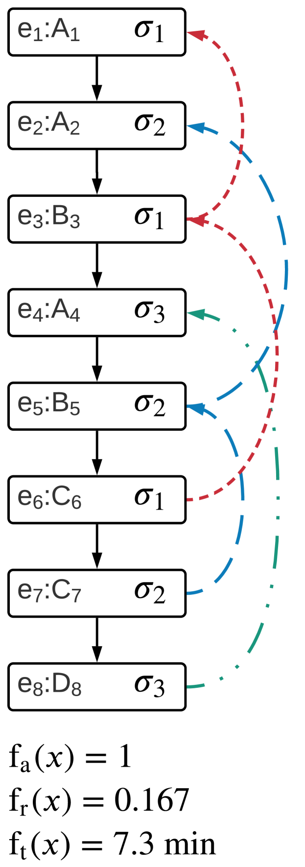
(a) Iteration 1 ($S_{\mathrm{curr}}=1$, $\uptau_{\mathrm{curr}}=100$, $\mathrm{prob}(x^{\prime})=0.99$)

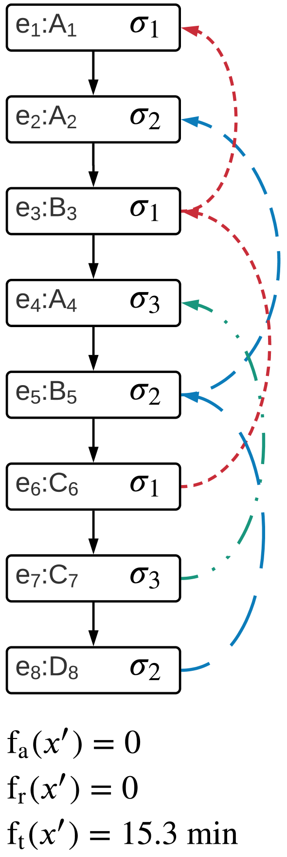
(b) Iteration 2 ($S_{\mathrm{curr}}=2$, $\uptau_{\mathrm{curr}}=144.9$, $\mathrm{prob}(x^{\prime})$ is irrelevant)

Figure 12: EC-SA-Data iterations, with $S_{\mathrm{max}}=$2$$ and $\uptau_{\mathrm{init}}=$100$$

In the following section, we discuss the measures we introduce to evaluate the accuracy of our technique based on a pair of logs. We will see next in Section 6 that the two logs correspond to a golden standard and the one originated by EC-SA-Data.

5 Quality measures

To assess the quality of our technique, we defined measures that quantify the output accuracy. They are based on criteria that compare pairs of logs. In particular, we can group our measures in two categories. The first category is the log-to-log similarity, which takes into account trace-based and case-based distances. The second category is log-to-log time deviation, determining the temporal distance of events’ elapsed times and cases’ cycle times. The definition of a complete set of measures to compare logs goes beyond the scope of this paper. The measures we propose here are inspired by related work in the literature [55, 52, 56, 57, 27, 18] and provide a good trade-off between run-time computability and different level of details used in the comparison, experimental results evidenced. A refinement and enrichment of this set can be part of future investigations.

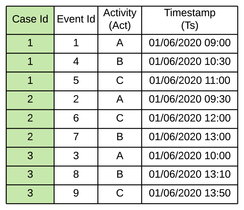
(a) Log $L$

(b) Log $L^{\prime}$

Figure 13: Event logs $L$ and $L^{\prime}$ for quality measures example

We use the two event logs in Fig. 13 to illustrate the different quality measures. We remark that our focus is on logs $L$ and $L^{\prime}$ that stem from the same uncorrelated log and case id’s, but possibly differ for the the way in which events are correlated. Therefore, the cardinality of case sets $S(L)$ and $S(L^{\prime})$ yet cases in $S(L)$ and $S(L^{\prime})$ may differ.

5.1 Log-to-log similarity

The log-to-log similarity category focuses on measuring the structure similarity between two logs from trace- and case-structure perspectives. This category is comprised of six measures. The values of those measures range from $0$ to $1$, where $1$ indicates the highest similarity. In the following, we describe the measures following an order given by a decreasing level of abstraction and aggregation with which the similarity between a pair of logs is established. The higher the level of detail, the more fine-granular differences are considered by the measure.

Inspired by the fitness measure proposed in [52], we define our first similarity measure, trace-to-trace similarity. It aims at assessing the extent to which two logs capture the same underlying control-flow through the string-edit distance of their traces. We formally define it as follows.

Definition 15 (Trace-to-trace similarity)

Let $L=(\mathrm{UL},I,\ell)$ and $L^{\prime}=(\mathrm{UL},I,\ell^{\prime})$ be two event logs. Let $\Delta^{\mathrm{ins}}_{\mathrm{del}}$ be the string-edit distance based on insertions and deletions [55]. We denote with $T=\{t_{1},t_{2},\ldots,t_{|T|}\}$ and $T^{\prime}=\{t^{\prime}_{1},t^{\prime}_{2},\ldots,t^{\prime}_{|T^{\prime}|}\}$ the set of distinct traces that are derived from event logs $L$ and $L^{\prime}$, respectively, i.e., $T=\bigcup_{\sigma\in S(L)}{\textrm{Act}(\sigma)}$ and $T^{\prime}=\bigcup_{\sigma^{\prime}\in S(L^{\prime})}{\textrm{Act}(\sigma^{\prime})}$. We indicate as the trace-closest trace to $t\in T$ a trace in $t^{\prime}_{\star}\in T^{\prime}$ derived as follows:

$$t^{\prime}_{\star}=\underset{t^{\prime}\in T^{\prime}}{\operatorname*{arg\,min}}\,\Big{\{}\Delta^{\mathrm{ins}}_{\mathrm{del}}\left(t,t^{\prime}\right)\Big{\}}$$ (14)

The trace-to-trace similarity $\mathrm{L2L_{trace}}$ is computed as follows:

$$\mathrm{L2L_{trace}}=1-\frac{\sum\limits_{t\in T}{\Delta^{\mathrm{ins}}_{\mathrm{del}}\left(t,t^{\prime}_{\star}\right)}}{\sum\limits_{t\in T}{\left(|t|+|t^{\prime}_{\star}|\right)}}$$ (15)

Table 2: Computation of $\mathrm{L2L_{trace}}$for logs $L$ and $L^{\prime}$ in Fig. 13

(a) Distinct traces in $L$

$t_{1}=\langle\mathsf{A},\mathsf{B},\mathsf{C}\rangle$ $t_{2}=\langle\mathsf{A},\mathsf{C},\mathsf{B}\rangle$

(b) Distinct traces in $L^{\prime}$

$t^{\prime}_{1}=\langle\mathsf{A},\mathsf{C},\mathsf{B}\rangle$ $t^{\prime}_{2}=\langle\mathsf{A},\mathsf{B},\mathsf{C}\rangle$

(c) Matching pair $(t_{\star},t^{\prime}_{\star})$ for each trace in $L$ and $L^{\prime}$

${\Delta^{\mathrm{ins}}_{\mathrm{del}}}(t_{1},t^{\prime}_{1})=1$ ${\Delta^{\mathrm{ins}}_{\mathrm{del}}}(t_{1},t^{\prime}_{2})=0$ ${\Delta^{\mathrm{ins}}_{\mathrm{del}}}(t_{2},t^{\prime}_{1})=0$ ${\Delta^{\mathrm{ins}}_{\mathrm{del}}}(t_{2},t^{\prime}_{2})=1$

For example, Table 2(a) shows two distinct traces in event log $L$ (depicted in Fig. 13(a)) and Table 2(b) shows two distinct traces in event log $L^{\prime}$ (Fig. 13(b)). The pairs of trace-closest traces $(t,t^{\prime}_{\star})$ are illustrated in Table 2(c). We select the pairs that minimize the total distance $\Delta_{\textrm{total}}$ between traces (see the marked cells in Table 2(c)). For instance, for $t_{1}$ we select the trace-closest pair $\left(t_{1},t^{\prime}_{2}\right)$ instead of $\left(t_{1},t^{\prime}_{1}\right)$ because the distance of the former $\Delta^{\mathrm{ins}}_{\mathrm{del}}\left(t_{1},t^{\prime}_{2}\right)=0$ is lower than $\Delta^{\mathrm{ins}}_{\mathrm{del}}\left(t_{1},t^{\prime}_{1}\right)=1$. Finally, we compute $\mathrm{L2L_{trace}}$ as a fraction having the sum of the string-edit distances between pairs of trace-closest traces ($0+0=0$) as the numerator and the length of the traces in $L$ and their trace-closest traces in $L^{\prime}$ ($k=|t_{1}|+|t^{\prime}_{2}|+|t_{2}|+|t^{\prime}_{1}|=12$) as the denominator.

The second measure we introduce is the trace-to-trace frequency similarity. It is more fine-granular than trace-to-trace similarity as it also takes into account the frequency with which traces occur. The formal definition follows.

Definition 16 (Trace-to-trace frequency similarity)

Let $L=(\mathrm{UL},I,\ell)$ and $L^{\prime}=(\mathrm{UL},I,\ell^{\prime})$ be two event logs, whose cases are $S(L)=\{\sigma_{1},\sigma_{2},\ldots,\sigma_{|I|}\}$ and $S(L^{\prime})=\{\sigma^{\prime}_{1},\sigma^{\prime}_{2},\ldots,\sigma^{\prime}_{|I|}\}$ respectively. Let $\Delta^{\mathrm{ins}}_{\mathrm{del}}$ be the string-edit distance based on insertions and deletions [55]. Let $\mathrm{tcc}:S(L)\to S(L^{\prime})$ be a bijective function mapping every case in $L$ to exactly one case in $L^{\prime}$, $\mathrm{TCC}$ the set of all possible such bijective functions definable having $S(L)$ and $S(L^{\prime})$ as domain and range respectively, and $\mathrm{tcc}_{\star}\in\mathrm{TCC}$ be such that the total string-edit distance between $\mathrm{tcc}_{\star}$-mapped pairs of cases is minimal:

$$\mathrm{tcc}_{\star}=\underset{\mathrm{tcc}\in\mathrm{TCC}}{\operatorname*{arg\,min}}\,\Big{\{}\sum\limits_{\sigma\in S(L)}\Delta^{\mathrm{ins}}_{\mathrm{del}}\left(\mathrm{Act}(\sigma),\mathrm{Act}(\mathrm{tcc}(\sigma))\right)\Big{\}}$$ (16)

Naming the $\mathrm{tcc}_{\star}$-mapped cases as trace-closest case pairs, let $\Delta_{\mathrm{total}}(L,L^{\prime})$ be the sum of all string-edit distances between trace-closest case pairs:

$$\Delta_{\mathrm{total}}=\sum\limits_{\sigma\in S(L)}\Delta^{\mathrm{ins}}_{\mathrm{del}}\left(\mathrm{Act}(\sigma),\mathrm{Act}(\mathrm{tcc}_{\star}(\sigma))\right)$$ (17)

The trace-to-trace frequency similarity, $\mathrm{L2L_{freq}}$, is the opposite of the average of the total distances between trace-closest case pairs:

$$\mathrm{L2L_{trace}}\!\left(L,L^{\prime}\right)=1-\frac{\Delta_{\mathrm{total}}}{2\times|E|}$$ (18)

Table 3: Computation of $\mathrm{L2L_{freq}}$for logs $L$ and $L^{\prime}$ in Fig. 13

(a) Traces in $L$

$\mathrm{Act}(\sigma_{1})=\langle\mathsf{A},\mathsf{B},\mathsf{C}\rangle$ $\mathrm{Act}(\sigma_{2})=\langle\mathsf{A},\mathsf{C},\mathsf{B}\rangle$ $\mathrm{Act}(\sigma_{3})=\langle\mathsf{A},\mathsf{B},\mathsf{C}\rangle$

(b) Traces in $L^{\prime}$

$\mathrm{Act}(\sigma^{\prime}_{1})=\langle\mathsf{A},\mathsf{B},\mathsf{C}\rangle$ $\mathrm{Act}(\sigma^{\prime}_{2})=\langle\mathsf{A},\mathsf{C},\mathsf{B}\rangle$ $\mathrm{Act}(\sigma^{\prime}_{3})=\langle\mathsf{A},\mathsf{C},\mathsf{B}\rangle$

(c) Matching pair $(\sigma_{\star},\sigma^{\prime}_{\star})$ for each trace in $L$ and $L^{\prime}$

${\Delta^{\mathrm{ins}}_{\mathrm{del}}}(\mathrm{Act}(\sigma_{1}),\mathrm{Act}(\sigma^{\prime}_{1}))=0$ ${\Delta^{\mathrm{ins}}_{\mathrm{del}}}(\mathrm{Act}(\sigma_{2}),\mathrm{Act}(\sigma^{\prime}_{1}))=2$ ${\Delta^{\mathrm{ins}}_{\mathrm{del}}}(\mathrm{Act}(\sigma_{3}),\mathrm{Act}(\sigma^{\prime}_{1}))=0$ ${\Delta^{\mathrm{ins}}_{\mathrm{del}}}(\mathrm{Act}(\sigma_{1}),\mathrm{Act}(\sigma^{\prime}_{2}))=2$ ${\Delta^{\mathrm{ins}}_{\mathrm{del}}}(\mathrm{Act}(\sigma_{2}),\mathrm{Act}(\sigma^{\prime}_{2}))=0$ ${\Delta^{\mathrm{ins}}_{\mathrm{del}}}(\mathrm{Act}(\sigma_{3}),\mathrm{Act}(\sigma^{\prime}_{2}))=2$ ${\Delta^{\mathrm{ins}}_{\mathrm{del}}}(\mathrm{Act}(\sigma_{1}),\mathrm{Act}(\sigma^{\prime}_{2}))=0$ ${\Delta^{\mathrm{ins}}_{\mathrm{del}}}(\mathrm{Act}(\sigma_{2}),\mathrm{Act}(\sigma^{\prime}_{3}))=0$ ${\Delta^{\mathrm{ins}}_{\mathrm{del}}}(\mathrm{Act}(\sigma_{3}),\mathrm{Act}(\sigma^{\prime}_{3}))=2$

To compute $\mathrm{tcc}_{\star}$ as in Eq. 16 and thus find the trace-closest case pairs, we use the Hungarian Algorithm [58]. For example, Table 3(a) shows the traces that stem from event log $L$ (depicted in Fig. 13(a)) and Table 2(b) shows the traces stemming from event log $L^{\prime}$ (depicted in Fig. 13(b)). Table 3(c) illustrates the pairs of trace-closest cases that we derive. The selected ones are colored in light blue: $\Delta^{\mathrm{ins}}_{\mathrm{del}}\left(\mathrm{Act}\left(\sigma_{1}\right),\mathrm{Act}\left(\sigma^{\prime}_{1}\right)\right)=0$, $\Delta^{\mathrm{ins}}_{\mathrm{del}}\left(\mathrm{Act}\left(\sigma_{2}\right),\mathrm{Act}\left(\sigma^{\prime}_{2}\right)\right)=0$, and $\Delta^{\mathrm{ins}}_{\mathrm{del}}\left(\mathrm{Act}\left(\sigma_{3}\right),\mathrm{Act}\left(\sigma^{\prime}_{3}\right)\right)=2$. These pairs lead to the minimum $\Delta_{\mathrm{total}}=2$. Finally, we compute $\mathrm{L2L_{freq}}=1-\frac{2}{2\times 9}=0.78$.

The following four measures investigate the similarity between logs at the level of events. Notice that we compare pairs of cases for which the first event correspond. The third measure we describe is the partial case similarity, which is based upon the number of events shared by cases that have the same first event.

Definition 17 (Partial case similarity)

Let $L=(\mathrm{UL},I,\ell)$ and $L^{\prime}=(\mathrm{UL},I,\ell^{\prime})$ be two event logs, whose case sets are $S(L)$ and $S(L^{\prime})$ respectively. We indicate with $\mathrm{intersect}:E^{*}\times E^{*}\to\mathbb{N}\cup{0}$ a function that takes two cases $\sigma$ and $\sigma^{\prime}$ as input and returns the number of events that $\sigma$ and $\sigma^{\prime}$ have in common.

$$\mathrm{intersect}\!\left(\sigma,\sigma^{\prime}\right)=\left|\left\{e\in\sigma:e\in\sigma^{\prime}\right\}\right|$$ (19)

The partial case similarity distance $\mathrm{L2L_{first}}$ averages the number of events in common (except the first one) that cases in $L$ and $L^{\prime}$ have when they share the same first event over the number of events in $L$ (except the first ones of the cases), as follows:

$$\mathrm{L2L_{first}}\!\left(L,L^{\prime}\right)=\frac{\underset{\begin{subarray}{c}\sigma\in S(L),\\ \sigma^{\prime}\in S(L^{\prime}):\\ \sigma(1)=\sigma^{\prime}(1)\end{subarray}}{\sum}{\mathrm{intersect}\!\left(\sigma\left[2,|\sigma|\right],\sigma^{\prime}\!\left[2,\left|\sigma^{\prime}\right|\right]\right)}}{|E|-|I|}$$ (20)

Table 4: Intersect between cases with the same start event in $L$ and $L^{\prime}$

$\mathrm{intersect}(\sigma_{1},\sigma^{\prime}_{1})=1$

$\mathrm{intersect}(\sigma_{2},\sigma^{\prime}_{2})=1$

$\mathrm{intersect}(\sigma_{3},\sigma^{\prime}_{3})=1$

For instance, given the event logs $L$ and $L^{\prime}$ in Figs. 13(a) and 13(b), we compute the elements of the sum in the numerator of $\mathrm{L2L_{first}}\left(L,L^{\prime}\right)$ as depicted in Table 4. In the example, $\sigma_{1}$ and $\sigma^{\prime}_{1}$ have the same start event $\mathsf{A_{1}}$, thus, we check the occurrence of events in $\sigma_{1}[2,3]$ in $\sigma^{\prime}_{1}[2,3]$ and find that only $\mathsf{B_{4}}$ occur in both cases, so $\mathrm{intersect}\left(\sigma_{1}[2,3],\sigma^{\prime}_{1}[2,3]\right)=1$. Finally, $\mathrm{L2L_{first}}$is computed by averaging the non-start events in common over the total number of the non-start events: $\mathrm{L2L_{first}}=\frac{1+1+1}{9-3}=0.5$.

The fourth measure we describe is the bigram similarity. Inspired by [15], it is based on the number of sequences of two events (henceforth, bigrams, i.e., n-grams of length $2$) that occur in both logs. We formally define it as follows.

Definition 18 (Bigram similarity)

Let $L=(\mathrm{UL},I,\ell)$ and $L^{\prime}=(\mathrm{UL},I,\ell^{\prime})$ be two event logs, whose case sets are $S(L)$ and $S(L^{\prime})$ respectively. We denote as $\mathrm{occurs2}(\langle e,e^{\prime}\rangle,L)$ the indicator function that returns $1$ if there exists a case $\sigma\in S(L)$ such that $\left\langle e,e^{\prime}\right\rangle$ is a segment of it:

The bigram similarity $\mathrm{L2L_{2gram}}$ is computed dividing by the cardinality of $S(L)$ the average of bigrams in the cases of $L$ that also occur in $L^{\prime}$ as follows:

Table 5: Computation of $\mathrm{L2L_{2gram}}$for logs $L$ and $L^{\prime}$ in Fig. 13

$\mathrm{occurs2}(\langle\mathsf{A_{1}},\mathsf{B_{4}}\rangle.L^{\prime})=1$	$\mathrm{occurs2}(\langle\mathsf{B_{4}},\mathsf{C_{5}}\rangle.L^{\prime})=0$
$\mathrm{occurs2}(\langle\mathsf{A_{2}},\mathsf{C_{6}}\rangle.L^{\prime})=0$	$\mathrm{occurs2}(\langle\mathsf{C_{6}},\mathsf{B_{7}}\rangle.L^{\prime})=0$
$\mathrm{occurs2}(\langle\mathsf{A_{3}},\mathsf{B_{8}}\rangle.L^{\prime})=0$	$\mathrm{occurs2}(\langle\mathsf{B_{8}},\mathsf{C_{9}}\rangle.L^{\prime})=0$

For example, for every pair ¨ in $L$ (depicted in Fig. 13(a)), we check if $\left\langle e,e^{\prime}\right\rangle$ occurs in $L^{\prime}$ (depicted in Fig. 13(b)) as shown in Table 5. Notice that $L$ and $L^{\prime}$ have only one bigram in common, that is $\langle\mathsf{A_{1}},\mathsf{B_{4}}\rangle$. Therefore, $\mathrm{L2L_{2gram}}$ = $\frac{1}{3}\left(\frac{1+0}{3-1}+\frac{0+0}{3-1}+\frac{0+0}{3-1}\right)=0.167$.

The fifth measure we describe is the trigram similarity, which extends the bigram similarity by considering n-grams of length $3$ (trigrams) in place of bigrams. We formally define it as follows.

Definition 19 (Trigram similarity)

Let $L=(\mathrm{UL},I,\ell)$ and $L^{\prime}=(\mathrm{UL},I,\ell^{\prime})$ be two event logs, whose case sets are $S(L)$ and $S(L^{\prime})$ respectively. We denote as $\mathrm{occurs3}(\langle e,e^{\prime},e^{\prime\prime}\rangle,L)$ the indicator function that returns $1$ if there exists a case $\sigma\in S(L)$ such that $\left\langle e,e^{\prime},e^{\prime\prime}\right\rangle$ is a segment of it.

The trigram similarity $\mathrm{L2L_{3gram}}$ is computed dividing by the cardinality of $S(L)$ the average of trigrams in the cases of $L$ that also occur in $L^{\prime}$ as follows:

Table 6: Computation of $\mathrm{L2L_{3gram}}$for logs $L$ and $L^{\prime}$ in Fig. 13

$\mathrm{occurs3}(\langle\mathsf{A_{1}},\mathsf{B_{4}},\mathsf{C_{5}}\rangle.L^{\prime})=0$

$\mathrm{occurs3}(\langle\mathsf{A_{2}},\mathsf{C_{6}},\mathsf{B_{7}}\rangle.L^{\prime})=0$

$\mathrm{occurs3}(\langle\mathsf{A_{3}},\mathsf{B_{8}},,\mathsf{C_{9}}\rangle.L^{\prime})=0$

For example, for every trigram $\langle e,e^{\prime},e^{\prime\prime}\rangle$ in $L$ (depicted in Fig. 13(a)), we check if it occurs in $L^{\prime}$ (depicted in Fig. 13(b)). As shown in Table 6, $L$ and $L^{\prime}$ do not have trigrams in common. Therefore, $\mathrm{L2L_{3gram}}=0$. If the case assignments of $e_{5}$ and $e_{6}$ were swapped (i.e., $e_{5}$ and $e_{6}$ had been assigned with $\sigma^{\prime}_{3}$ and $\sigma^{\prime}_{2}$, respectively), then the value of $\mathrm{L2L_{3gram}}$ would be $\frac{1}{3}$.

The last measure we describe is the case similarity, which checks the extent to which a pair of logs identically correlate cases as a whole. We formally define it as follows.

Definition 20 (Case similarity, $\mathrm{L2L_{case}}$)

Let $L=(\mathrm{UL},I,\ell)$ and $L^{\prime}=(\mathrm{UL},I,\ell^{\prime})$ be two event logs, whose case sets are $S(L)$ and $S(L^{\prime})$ respectively. The case similarity, $\mathrm{L2L_{case}}$, amounts to the number of cases that are equal in $L$ and $L^{\prime}$ divided by the total number of cases:

$$\mathrm{L2L_{case}}\!\left(L,L^{\prime}\right)=\frac{\left|S(L)\cap S(L^{\prime})\right|}{|I|}$$ (25)

Notice that we indicate with $S(L)\cap S(L^{\prime})$ the cases in $L$ that have an equal one in $L^{\prime}$. As the number of cases is the same in $L$ and $L^{\prime}$, $\mathrm{L2L_{case}}$ can be considered as a Sørensen-Dice coefficient for $S(L)$ and $S(L^{\prime})$ [56]. In the example, given $L$ (depicted in Fig. 13(a)) and $L^{\prime}$ (depicted in Fig. 13(b)), there are no equal cases occurring in $L$ and $L^{\prime}$. Therefore, $\mathrm{L2L_{case}}=0$. If the case assignments of $e_{5}$ and $e_{6}$ were swapped (i.e., $\ell(e_{5})=\sigma^{\prime}_{3}$ and $\ell(e_{6})=\sigma^{\prime}_{2}$), then the value of $\mathrm{L2L_{case}}$ would be $\frac{1}{3}$.

Up to this point, we have presented the measures following an order given by the increasing amount of details they consider in the comparison. We shall refer to the ones at a higher level of abstraction as more relaxed (e.g., $\mathrm{L2L_{trace}}$), as opposed to the stricter ones (e.g., $\mathrm{L2L_{case}}$). In the following, we present measures that deal with time deviations.

5.2 Log-to-log time deviation

The log-to-log time deviation category consists of two measures which use the symmetric mean absolute percentage error (SMAPE) to compute the time deviation between a pair of logs. Their values range from $0$ to $1$, where $0$ indicates the highest similarity between the two logs.

The first measure we describe here is the event time deviation. It investigates the extent to which the two logs deviate in terms of the elapsed time of events. We formally define it as follows.

Definition 21 (Event time deviation)

Let $L=(\mathrm{UL},I,\ell)$ and $L^{\prime}=(\mathrm{UL},I,\ell^{\prime})$ be two event logs defined over a common universe of events $E$. Let $\mathrm{ET}(\sigma,e)$ be the elapsed time (ET) of event $e$ in case $\sigma$ as per Eq. 8. The event time deviation, $\mathrm{SMAPE_{ET}}$, is the Symmetric Mean Absolute Percentage Error (SMAPE) of the elapsed time of events between $L$ and $L^{\prime}$, computed as follows:
$\displaystyle\mathrm{SMAPE_{ET}}(L,L^{\prime})=$ $\displaystyle\frac{\sum_{e\in E}{\frac{\left|\mathrm{ET}(\sigma,e)-\mathrm{ET}(\sigma^{\prime},e)\right|}{|\mathrm{ET}(\sigma,e)|+|\mathrm{ET}(\sigma^{\prime},e)|}}}{|E|-|I|}$ $\displaystyle\textrm{with}\>\sigma=L(\ell(e)),\;\sigma^{\prime}=L^{\prime}(\ell(e))$ (26)

Table 7: Computation of $\mathrm{SMAPE_{ET}}$ for logs $L$ and $L^{\prime}$ in Fig. 13

(a) Elapsed time (in min) of events in $L$

$\mathrm{ET}(\sigma_{1},\mathsf{B_{4}})=90$ $\mathrm{ET}(\sigma_{1},\mathsf{C_{5}})=30$ $\mathrm{ET}(\sigma_{1},\mathsf{C_{6}})=150$ $\mathrm{ET}(\sigma_{1},\mathsf{B_{7}})=60$ $\mathrm{ET}(\sigma_{1},\mathsf{B_{8}})=190$ $\mathrm{ET}(\sigma_{1},\mathsf{C_{9}})=40$

(b) Elapsed time (in min) of events in $L^{\prime}$

$\mathrm{ET}(\sigma_{1}^{\prime},\mathsf{B_{4}})=90$ $\mathrm{ET}(\sigma_{1}^{\prime},\mathsf{C_{5}})=90$ $\mathrm{ET}(\sigma_{1}^{\prime},\mathsf{C_{6}})=120$ $\mathrm{ET}(\sigma_{1}^{\prime},\mathsf{B_{7}})=120$ $\mathrm{ET}(\sigma_{1}^{\prime},\mathsf{B_{8}})=70$ $\mathrm{ET}(\sigma_{1}^{\prime},\mathsf{C_{9}})=200$

For example, the elapsed time of $\mathsf{C_{5}}$ in $L$, given that $L(\ell(\mathsf{C_{5}}))=\sigma_{1}$, is $\mathsf{C_{5}}.\mathrm{Ts}-\mathsf{B_{4}}.\mathrm{Ts}=$30\text{\,}\mathrm{min}$$, whereas the elapsed time of $\mathsf{C_{5}}$ in $L^{\prime}$, given that $L^{\prime}(\ell(\mathsf{C_{5}}))=\sigma^{\prime}_{2}$, is $\mathsf{C_{5}}.\mathrm{Ts}-\mathsf{A_{2}}.\mathrm{Ts}=$90\text{\,}\mathrm{min}$$. We compute $\mathrm{SMAPE_{ET}}$ using the elapsed time of the events in $L$ (depicted in Fig. 13(a)), and the elapsed time of the events in $L^{\prime}$ (depicted in Fig. 13(b)) as shown in Table 7. As a result, $\mathrm{SMAPE_{ET}}=0.35$.

The second measure we describe is the case cycle time deviation, assessing the extent to which two logs differ in terms of the cases’ cycle time. To compare pairs of cases, we consider those that begin with the same start event, as seen in Section 5.1 with $\mathrm{L2L_{first}}$. We formally define the measure as follows.

Definition 22 (Case cycle time deviation)

Let $L=(\mathrm{UL},I,\ell)$ and $L^{\prime}=(\mathrm{UL},I,\ell^{\prime})$ be two event logs defined over a common universe of events $E$. Let $\mathrm{CT}(\sigma)$ be the cycle time of case $\sigma$, computed as follows [59, 60]:

$$\mathrm{CT}(\sigma)=\sigma(|\sigma|).Ts-\sigma(1).Ts$$ (27)

The case cycle time deviation $\mathrm{SMAPE_{CT}}$ is the symmetric mean absolute percentage error of the cycle time between cases in $L$ and $L^{\prime}$:

$$\mathrm{SMAPE_{CT}}(L,L^{\prime})=\frac{1}{|I|}\times{\sum_{\begin{subarray}{c}\sigma\in L,\\ \sigma^{\prime}inL^{\prime}:\\ \sigma(1)=\sigma^{\prime}(1)\end{subarray}}{\frac{\left|\mathrm{CT}(\sigma)-\mathrm{CT}(\sigma^{\prime})\right|}{|\mathrm{CT}(\sigma)|+|\mathrm{CT}(\sigma^{\prime})|}}}$$ (28)

Table 8: Computation of $\mathrm{SMAPE_{CT}}$ for logs $L$ and $L^{\prime}$ in Fig. 13

(a) Cycle time (in hours) of events in $L$

$\mathrm{CT}(\sigma_{1})=\mathsf{C_{5}}.\mathrm{Ts}-\mathsf{A_{1}}.\mathrm{Ts}=1$ $\mathrm{CT}(\sigma_{2})=\mathsf{B_{7}}.\mathrm{Ts}-\mathsf{A_{2}}.\mathrm{Ts}=3.5$ $\mathrm{CT}(\sigma_{3})=\mathsf{C_{9}}.\mathrm{Ts}-\mathsf{A_{3}}.\mathrm{Ts}=3.8$

(b) Cycle time (in hours) of events in $L^{\prime}$

$\mathrm{CT}(\sigma^{\prime}_{1})=\mathsf{C_{9}}.\mathrm{Ts}-\mathsf{A_{1}}.\mathrm{Ts}=4.8$ $\mathrm{CT}(\sigma^{\prime}_{2})=\mathsf{B_{7}}.\mathrm{Ts}-\mathsf{A_{2}}.\mathrm{Ts}=3.5$ $\mathrm{CT}(\sigma^{\prime}_{3})=\mathsf{B_{8}}.\mathrm{Ts}-\mathsf{A_{3}}.\mathrm{Ts}=3.17$

For example, we compute the cycle time of case $\sigma_{1}$ in $L$ based on the first and the last events in the case: $\mathrm{CT}(\sigma_{1})=\mathsf{C_{5}}.\mathrm{Ts}-\mathsf{A_{1}}.\mathrm{Ts}=$1\text{\,}\mathrm{h}$$. The cycle time of case $\sigma^{\prime}_{1}$ in $L^{\prime}$ is $\mathrm{CT}(\sigma^{\prime}_{1})$ = $\mathsf{C_{9}}.\mathrm{Ts}-\mathsf{A_{1}}.\mathrm{Ts}=$4.8\text{\,}\mathrm{h}$$. We compute $\mathrm{SMAPE_{CT}}$ comparing the cycle time of the cases in event log $L$ (depicted in Fig. 13(a)) and the ones in event log $L^{\prime}$ (depicted in Fig. 13(b)) having the same start event, as shown in Table 8. As a result, $\mathrm{SMAPE_{CT}}=0.25$.

Thus far, we have presented the measures we use to assess the outcome of our approach. Next, we illustrate our experimental results and evaluate them by means of the aforementioned measures.

6 Evaluation

We implemented a prototype tool for EC-SA-Data. Using this tool, we conducted three experiments to evaluate the accuracy and time performance of our approach, and compared the results with EC-SA [18] used as a baseline.

6.1 Design

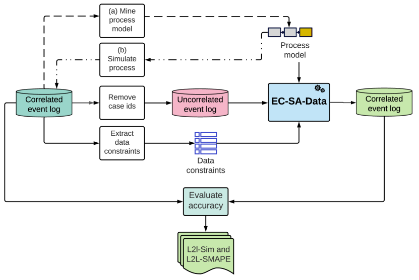
Figure 14: Evaluation steps

Figure 14 illustrates our evaluation process. The primary input is a correlated event log with defined cases; we refer to it as the original log. We remove the case identifiers from it and thereby create an uncorrelated event log. Thereupon, we run our implemented technique and measure its accuracy using the two categories of measures defined in Section 5. The first category is the log-to-log similarity, which assesses the extent to which EC-SA-Data generates a correlated log (we refer to it as $L^{\prime}$ in Def.s 15, 16, 17, 18, 19, 20, 21 and 22) that is consistent with the original log (we refer to it as $L$ in Def.s 15, 16, 17, 18, 19, 20, 21 and 22) in terms of trace-based and case-based distances. The second category is log-to-log time deviation, which considers the temporal distance of events’ elapsed times and cases’ cycle times.

The three experiments differ in terms of their input and research objectives. Overall, we aim to assess the effectiveness of our technique, taking into account evaluation principles as described in [61].

The first experiment performs a sensitivity analysis on the impact on the accuracy of the output log that increasing the number of cases overall and of the average work-in-progress cases (WIP, i.e., the density of the overlapping cases at a point in time) entails. We tuned the inter-arrival time between starting cases to setup the WIP. To generate the input logs, we simulated a process that includes basic process behavior patterns, i.e., sequence, concurrency, exclusiveness, and cyclic runs. The produced logs present the following characteristics: (a) a varying number of cases, ranging between $100$ and $1000$ at steps of $100$; (b) different inter-arrival time based on the cycle time (CT) of the process (i.e., the time spent by a case from start to end), ranging between $\nicefrac{{\textrm{CT}}}{{32}}$ and CT, at multiplicative steps of $2$.

	Traces		Events		Trace length
Event log	Total	Dst.%	Total	Dst.%	Min	Avg	Max
BPIC13cp [62]	$1487$	$12.3$	$6660$	$7$	$1$	$4$	$35$
BPIC13inc [63]	$7554$	$20.0$	$65\,533$	$13$	$1$	$9$	$123$
BPIC151f [64]	$902$	$32.7$	$21\,656$	$70$	$5$	$24$	$50$
BPIC17f [65]	$21\,861$	$40.1$	$714\,198$	$41$	$11$	$33$	$113$

Table 9: Descriptive statistics of real logs

Event log	Equality constraints	IF-THEN constraints
BPIC13cp [62]	$3$	$3$
BPIC13inc [63]	$3$	$2$
BPIC151f [64]	$4$	$0$
BPIC17f [65]	$3$	$7$

Table 10: Data constraints per event log

The second experiment assesses the accuracy improvement our approach yields when data constraints are provided together with an input process model. For this experiment, we used four real-world datasets from the benchmark of Augusto et al. [66] based on the publicly available event logs in the BPIC repository. Table 9 shows some descriptive statistics about them. We mined the process models from the original logs using a state-of-the-art discovery technique, namely Split Miner [11]. We extracted the data constraints by visual inspection and analysis of those event logs – Table 10 summarizes our findings. Thereupon, we compared the results attained with our approach with those of EC-SA, as the latter does not provide the capability of including data constraints to steer the assignment of case identifiers to the events.

The third experiment performs a sensitivity analysis that investigates the effect of the constraints on the accuracy of the log generated by EC-SA-Data. We used the BPIC17 event log [65] as filtered by Augusto et al. [66] (hence the ‘f’ subscript in “BPIC17_f” in the tables and figures), as we observed that a relatively high number of data constraints define its behavior, compared to other real-world event logs as shown in Table 10. In particular, we inferred ten rules that regulate the behavior of the process behind the BPIC17 log (see Appendix A). There are three data-attribute equality rules and seven IF-THEN constraints. Six IF-THEN rules are based on the matching of the operating resources over some activities within a case. The seventh IF-THEN rule is a correlation rule based on the equality of two different data attributes over some activities within a case.

This experiment investigates two aspects. The first aspect pertains to the effect of an increase in the number of used constraints on the accuracy of the generated log. We gradually increase the number of used constraints from zero to ten. Notice that the order of the constraints does not affect the accuracy of the output. Thereby, we investigate the impact of increasing the knowledge on the accuracy of the generated logs.

The second aspect concerns the impact of the knowledge quality on the accuracy of the generated logs. We impersonate the business analysts in their iterative endeavor. While inspecting the data, some rules occur as evident. Other ones are less certain or harder to confirm. Nevertheless, they could use all of them in an attempt to drive the automated correlation, although some could possibly misrepresent the data, thereby misleading the technique. To mimic this situation, we run successive tests adding (a) four correct rules (three of which are data-attribute equality constraints and one is an IF-THEN constraint), and then (b) three inexact rules. Notice that we omit three correct rules out of the ten aforementioned ones to mimic the missing knowledge.

Next, we describe in details the measures we used to evaluate accuracy and the results of our experiments.

6.2 Results

Figures 15 and 16 plot the results of the first experiment, which studies the impact of increasing log size and WIP on the accuracy of EC-SA-Data. As we detail in the following, we observe that the stricter the measure is, the steeper the decline gets as those parameters increase.

Figure 15 shows how log size and WIP affect log-to-log similarity measures. Markedly, a relaxed similarity measure such as $\mathrm{L2L_{trace}}$ drops by around $4\text{\,}\mathrm{\char 37\relax}$ from the situation in which logs consist of $100$ cases to when logs contain $1000$ cases, as shown in Fig. 15(a). Also, $\mathrm{L2L_{trace}}$ drops by around $2\text{\,}\mathrm{\char 37\relax}$ when the inter-arrival rate goes from a value that equates the process cycle time ($1$ CT) to one thirty-second thereof ($\nicefrac{{1}}{{32}}$ CT). The $\mathrm{L2L_{2gram}}$ similarity measure decreases by around $5\text{\,}\mathrm{\char 37\relax}$ having logs whose cardinality increases from $100$ cases to $1000$ cases. Also, its value decreases by around $3\text{\,}\mathrm{\char 37\relax}$ as the inter-arrival rate goes from $1$ CT to $\nicefrac{{1}}{{32}}$ CT, as shown in Fig. 15(d). The strictest similarity measure, $\mathrm{L2L_{case}}$, falls by around $19\text{\,}\mathrm{\char 37\relax}$ when cases increase from $100$ to $1000$, as shown in Fig. 15(f) and by around $18\text{\,}\mathrm{\char 37\relax}$ as the inter-arrival rate reaches a thirty-second of the process cycle time from the initial value of a whole cycle time.

Figure 16 illustrates how log size and WIP affect log-to-log time deviation measures. As Fig. 16(a) depicts, $\mathrm{SMAPE_{ET}}$ and $\mathrm{SMAPE_{CT}}$ drop by around $14\text{\,}\mathrm{\char 37\relax}$ and $13\text{\,}\mathrm{\char 37\relax}$, respectively, when the number of cases in the logs decreases from $100$ to $1000$. $\mathrm{SMAPE_{ET}}$ and $\mathrm{SMAPE_{CT}}$ drops by around $8\text{\,}\mathrm{\char 37\relax}$ and $15\text{\,}\mathrm{\char 37\relax}$, respectively, as the inter-arrival goes from $1$ CT to $\nicefrac{{1}}{{32}}$ CT, as shown in Fig. 16(b).

These drops occur because bigger logs bring more options to assign events with, and the inter-arrival rate has an influence on the number of overlapping cases. The combination of higher volumes of cases and their density increases the uncertainty of the correlation decision step, thereby affecting the accuracy of the technique.

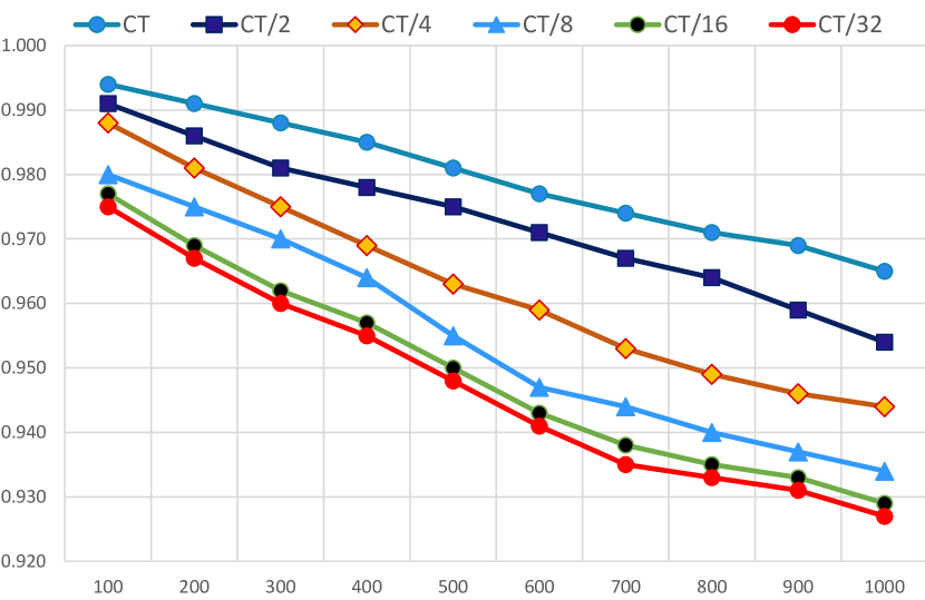
(a) EC-SA-Data- $\mathrm{L2L_{trace}}$

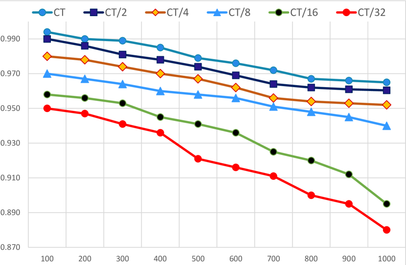
(b) $\mathrm{L2L_{freq}}$

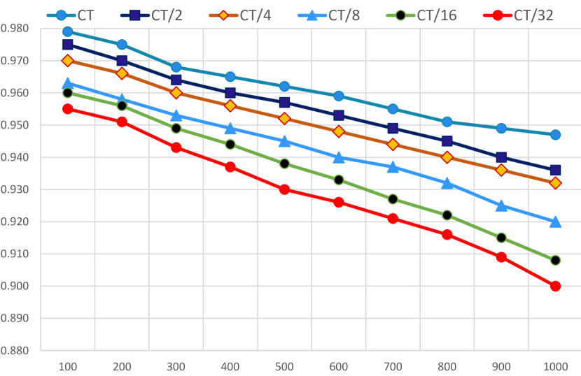
(c) $\mathrm{L2L_{first}}$

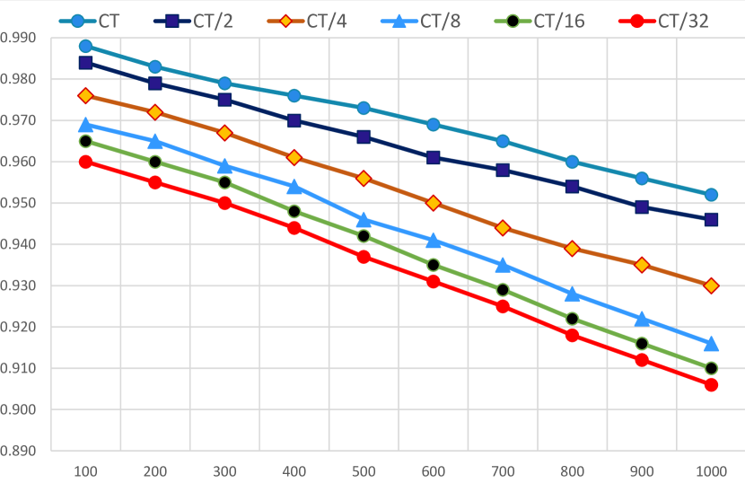
(d) $\mathrm{L2L_{2gram}}$

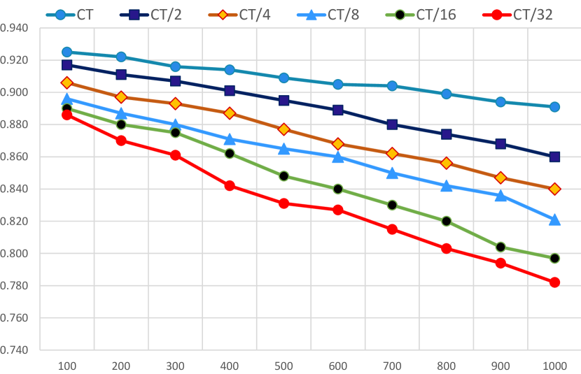
(e) $\mathrm{L2L_{3gram}}$

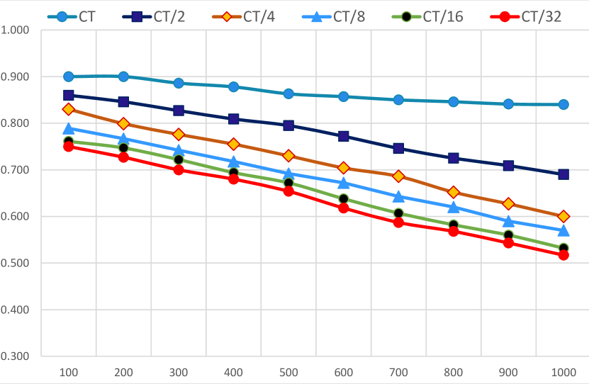
(f) $\mathrm{L2L_{case}}$

Figure 15: The impact of increasing log size (on the horizontal axis) and WIP (differentiated by the color and shape of the poly-lines) on log-to-log similarity measures (on the vertical axis)

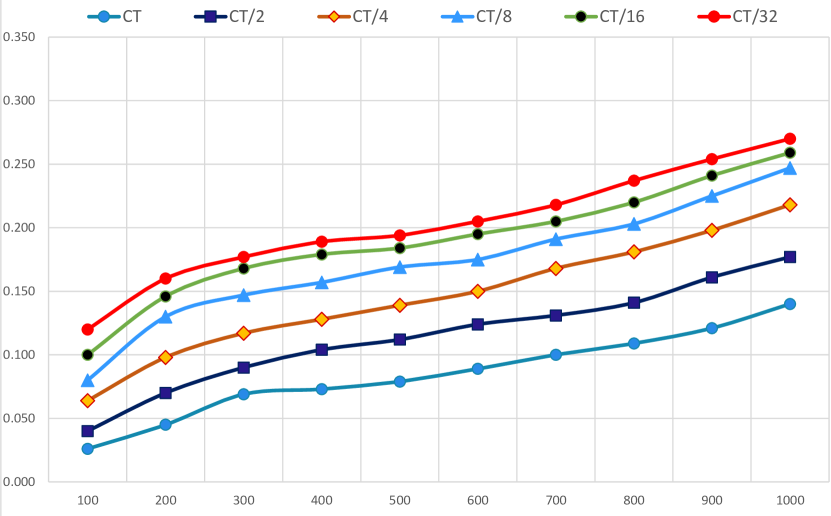
(a) $\mathrm{SMAPE_{ET}}$

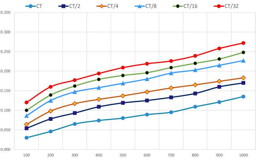
(b) $\mathrm{SMAPE_{CT}}$

Figure 16: The impact of increasing log size (on the horizontal axis) and WIP (differentiated by the color and shape of the poly-lines) on log-to-log time deviation measures (on the vertical axis)

Figures 17 and 18 show the results of the second experiment, which studies the impact that adding data constraints has on the correlation accuracy and compares the results with EC-SA (which, in contrast, did not allow for the inclusion of constraints). We can see that doing so improves the accuracy and, indeed, EC-SA-Data outperforms EC-SA. Figure 17 shows that $\mathrm{L2L_{trace}}$, $\mathrm{L2L_{2gram}}$ and $\mathrm{L2L_{case}}$ increase by around $6\text{\,}\mathrm{\char 37\relax}15\text{\,}\mathrm{\char 37\relax}28\text{\,}\mathrm{\char 37\relax}$ on average when constraints are in use, respectively. Notably, using data constraints with EC-SA-Data on the BPIC17 log dramatically improves the event correlation quality as it can be observed in Fig. 17(f) – notice that $\mathrm{L2L_{case}}$ increases by $46\text{\,}\mathrm{\char 37\relax}$. Figure 18 evidences that also the time deviation decreases when constraints are in use, as $\mathrm{SMAPE_{ET}}$ and $\mathrm{SMAPE_{CT}}$ rise by $19\text{\,}\mathrm{\char 37\relax}21\text{\,}\mathrm{\char 37\relax}$, respectively.

Using constraints enhances the correlation process as they prune out the violating options for case assignment. Consequently, the uncertainty of the correlation decision step decreases and this positively affects the quality of the generated log. However, the usage of data constraints affects the performance of EC-SA-Data particularly in terms of execution time. The reason is, constraints must be verified at every assignment step. Therefore, the more the constraints to check, the higher the overall computation time. For instance, EC-SA-Data ran for $13\text{\,}\mathrm{h}$ to complete the execution with the BPIC17 event log using $10$ constraints, in contrast with the $8.6\text{\,}\mathrm{h}$ needed in absence of constraints. The processing of the BPIC15_1f log required $6.2\text{\,}\mathrm{h}$ with $4$ constraints and $5.5\text{\,}\mathrm{h}$ without constraints.

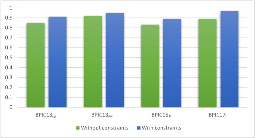
(a) $\mathrm{L2L_{trace}}$

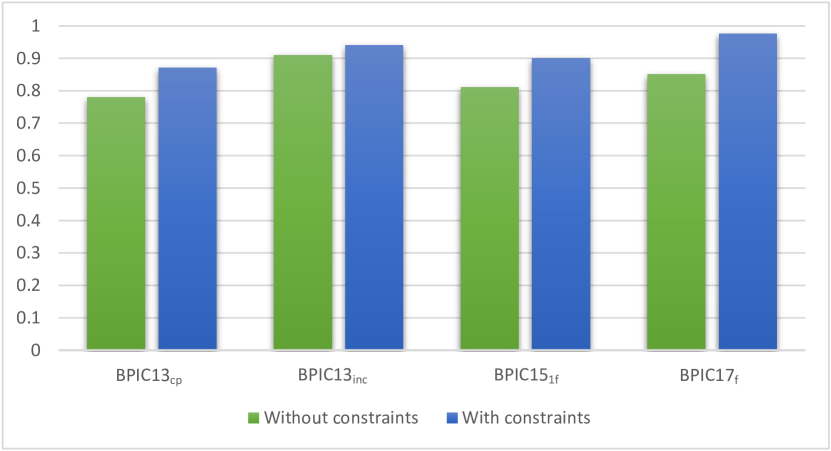
(b) $\mathrm{L2L_{freq}}$

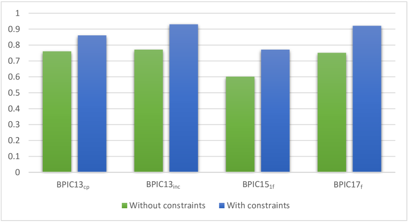
(c) $\mathrm{L2L_{first}}$

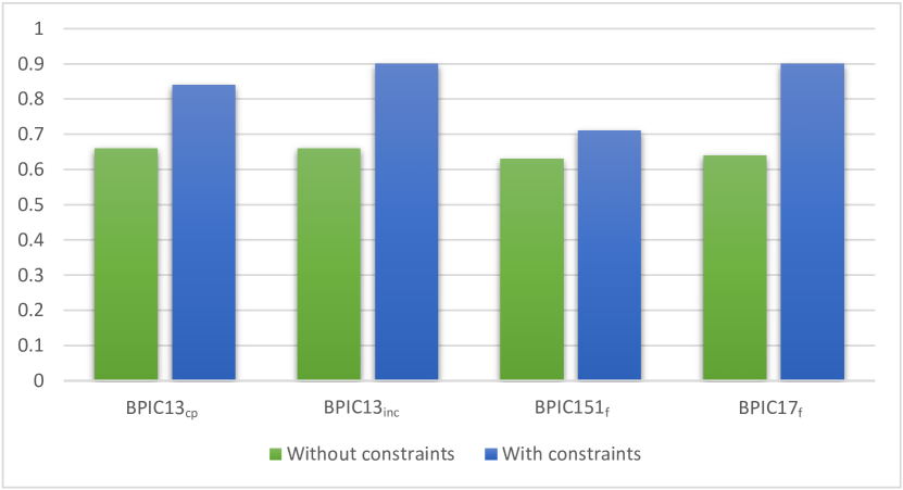
(d) $\mathrm{L2L_{2gram}}$

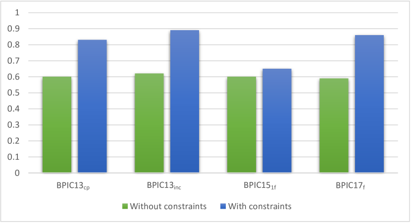
(e) $\mathrm{L2L_{3gram}}$

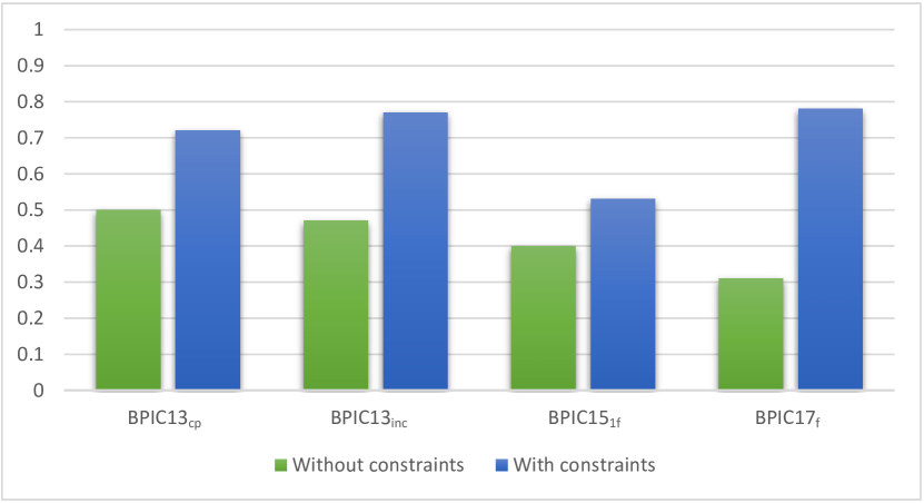
(f) $\mathrm{L2L_{case}}$

Figure 17: Impact of using data constraints with real-world logs on log-to-log similarity measures

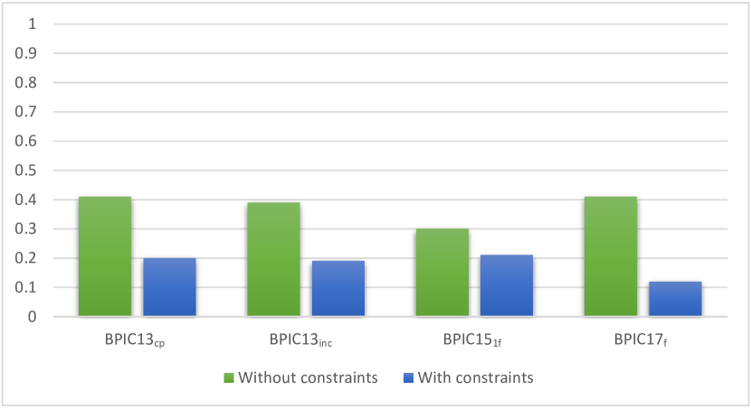
(a) $\mathrm{SMAPE_{ET}}$

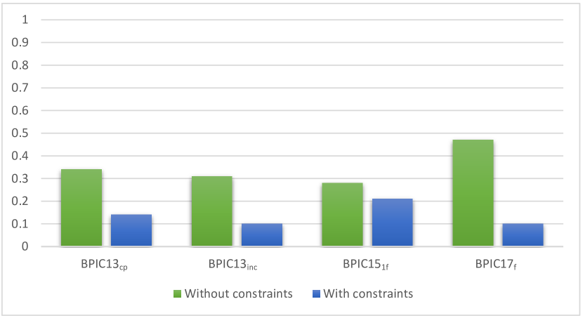
(b) $\mathrm{SMAPE_{CT}}$

Figure 18: Impact of using data constraints with real-world logs on time deviation measures

Figure 19 shows the results of the third experiment, which studies the effect of the number and correctness of constraints on the accuracy of the correlation process of EC-SA-Data. Figure 19(a) shows that using more constraints improves the log-to-log similarity accuracy measures of the generated logs. For instance, $\mathrm{L2L_{trace}}$, $\mathrm{L2L_{2gram}}$ and $\mathrm{L2L_{case}}$ increase by around $8\text{\,}\mathrm{\char 37\relax}24\text{\,}\mathrm{\char 37\relax}46\text{\,}\mathrm{\char 37\relax}$ when the constraints reach the peak of $10$ correct ones. Figure 19(b) evidences that the log-to-log time deviation accuracy measures decrease too: in particular, $\mathrm{SMAPE_{ET}}$ and $\mathrm{SMAPE_{CT}}$ drop by up to $36\text{\,}\mathrm{\char 37\relax}40\text{\,}\mathrm{\char 37\relax}$, respectively. These improvements materialize as more knowledge in terms of data constraints helps to discard event-case assignment possibilities and, therefore, decrease the uncertainty of the correlation decision.

Figures 19(c) and 19(d) illustrate the effect of using incorrect constraints. These constraints are intentionally inconsistent with data in order to study the impact of the knowledge quality on the accuracy of the technique. We observe that using $3$ wrong constraints makes $\mathrm{L2L_{trace}}$ reduce by $1\text{\,}\mathrm{\char 37\relax}$, $\mathrm{L2L_{2gram}}$ by $4\text{\,}\mathrm{\char 37\relax}$ and $\mathrm{L2L_{case}}$ by $5\text{\,}\mathrm{\char 37\relax}$. Also, it affects the time deviation measures as $\mathrm{SMAPE_{ET}}$ and $\mathrm{SMAPE_{CT}}$ increase by $4\text{\,}\mathrm{\char 37\relax}2\text{\,}\mathrm{\char 37\relax}$, respectively. We observe that invalid constraints affect the overall accuracy though not severely thanks to the positive impact of other valid ones. This scenario is meant to resemble a realistic scenario in which constraints are available but without the certainty that all of those are consistent with the event data at hand. We can see that EC-SA-Data still provides a valid correlated log with sufficient accuracy.

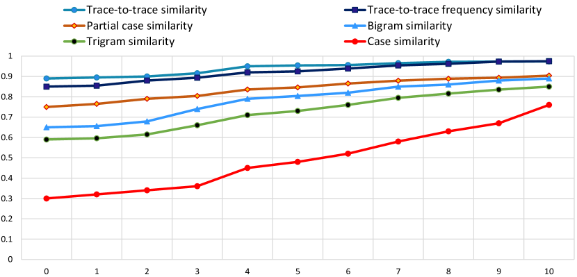
(a) Log similarity measures

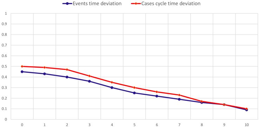
(b) Time variance measures

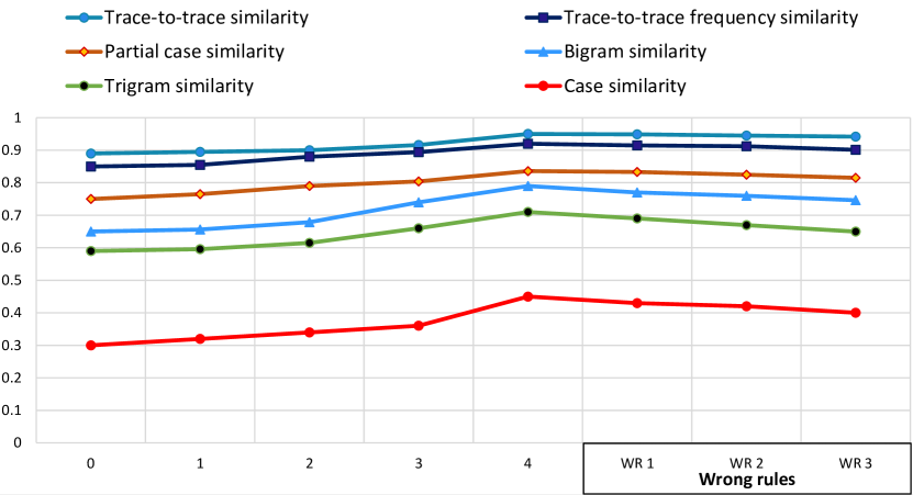
(c) Log similarity measures – using wrong rules

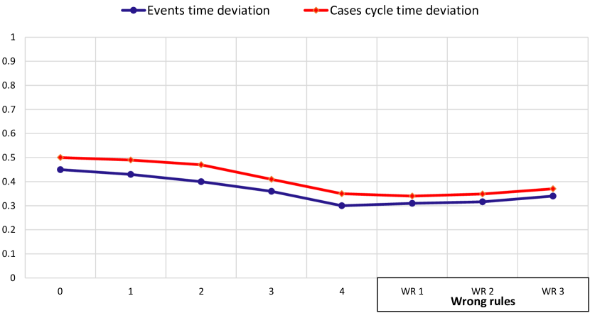
(d) Time variance measures – using wrong rules

Figure 19: Sensitivity analysis on the usage of constraints

6.3 Discussion

Based on the different sensitivity analyses we conducted, we found that using constraints improves correlation accuracy due to a reduction of possible assignments per event. Also, we see that by using constraints, we reduce the arbitrary decisions taken based on lowly accurate models. Our approach is mildly sensitive to the accuracy of the given data. The usage of various constraints with different support and correctness influence the event correlation decision. However, based on the third experiment, the correctness of some rules can balance the negative impact of the incorrect ones so as not to dramatically affect the correlation process. The accuracy of our approach tends to be partially prone to a worsening when the cases’ density and log size increase, as these parameters increase the number of options available thereby reducing certainty in the event assigning decision.

We remark that EC-SA-Data can handle cyclic and parallel behavior, largely present in the real-world event logs we analyzed, as opposed to other proposed techniques [15, 16, 26].. Also, EC-SA-Data allows users to provide rules that constrain the process behavior; however, it still consider those rules as a complement to the control-flow knowledge in order not to be entirely dependent on the accuracy of the event log data, as discussed in Section 2. Thus, combining the control-flow and data-domain knowledge helps to balance the inaccuracy of the input data and supports the correlation process in generating a sufficiently reliable output log. The investigation of possible solutions solely resorting to constraints paves the path for future work, as we will discuss in the next section.

7 Conclusion

The research presented in this paper addresses the event correlation problem. To automatically correlate the events to their proper cases, our approach (EC-SA-Data) resorts to data constraints to model domain knowledge, in addition to process models that define the control-flow of the original process. Our approach uses multi-level objective simulated annealing to map every event to a case. We use trace alignment cost, support of data constraints, and activity execution time variance for optimization. Our evaluation on real-world event logs demonstrates that using data constraints as input in addition to the process model improves the generated log quality positively.

There are several directions for future research. A first option is to support a broader spectrum of data knowledge constraints, such as the inter-case constraints [67]. Also, extending the set of quality measures for correlated event logs is an objective that can be pursued in following endeavors. Finally, an interesting avenue for future work is to explore the possibility of correlating the events solely based on constraints, without prior knowledge of the whole process model or by means of declarative process rules [68].

Acknowledgements

The work of Claudio Di Ciccio was partly supported by the Italian Ministry of University and Research (MUR) under grant “Dipartimenti di eccellenza 2018-2022” of the Department of Computer Science at Sapienza University of Rome and by the Sapienza SPECTRA research project. The research by Jan Mendling was supported by the Einstein Foundation Berlin.

Appendix A BPIC-2017 rules

Table 11 reports the data constraints we retrieved from visual inspection of the BPIC17_f event log to run our experiments.

$C_{1}:\sigma(i-1).\mathrm{ApplicationType}=\sigma(i).\mathrm{ApplicationType}$

$C_{2}:\sigma(i-1).\mathrm{LoanGoal}=\sigma(i).\mathrm{LoanGoal}$

$C_{3}:\sigma(i-1).\mathrm{RequestedAmount}=\sigma(i).\mathrm{RequestedAmount}$

$C_{4}:\texttt{IF}\leavevmode\nobreak\ \sigma(i).\mathrm{EventOrigin}=\textrm{``}\textsf{Offer}\textrm{''}\wedge \sigma(i).\mathrm{Act} \neq \textrm{``}\textsf{O\_Create\leavevmode\nobreak\ offer}\textrm{''}\wedge\sigma(j).\mathrm{Act}=  \textrm{``}\textsf{O\_Create\leavevmode\nobreak\ offer}\textrm{''}\leavevmode\nobreak\ \texttt{THEN}\leavevmode\nobreak\ \sigma(i).\mathrm{OfferID}=\sigma(j).\mathrm{EventId}$

$C_{5}:\texttt{IF}\leavevmode\nobreak\ \sigma(i).\mathrm{Act}=\textrm{``}\textsf{A\_Complete}\textrm{''}\wedge\sigma(j).\mathrm{Act}=  \textrm{``}\textsf{W\_Call\leavevmode\nobreak\ after\leavevmode\nobreak\ offers}\textrm{''}\leavevmode\nobreak\ \texttt{THEN}\leavevmode\nobreak\ \sigma(i).\mathrm{Resource}=\sigma(j).\mathrm{Resource}$

$C_{6}:\texttt{IF}\leavevmode\nobreak\ \sigma(i).\mathrm{Act}= \textrm{``}\textsf{W\_Call\leavevmode\nobreak\ after\leavevmode\nobreak\ offers}\textrm{''} \wedge \sigma(i).\mathrm{Act}= \textrm{``}\textsf{O\_Sent\leavevmode\nobreak\ (mail\leavevmode\nobreak\ and\leavevmode\nobreak\ online)}\textrm{''} \leavevmode\nobreak\ \texttt{THEN}\leavevmode\nobreak\ \sigma(i).\mathrm{Resource}=\sigma(j).\mathrm{Resource}$

$C_{7}:\texttt{IF}\leavevmode\nobreak\ \sigma(i).\mathrm{Act}= \textrm{``}\textsf{O\_Returned}\textrm{''} \wedge \sigma(i).\mathrm{Act}= \textrm{``}\textsf{A\_Validating}\textrm{''} \leavevmode\nobreak\ \texttt{THEN}\leavevmode\nobreak\ \sigma(i).\mathrm{Resource}=\sigma(j).\mathrm{Resource}$

$C_{8}:\texttt{IF}\leavevmode\nobreak\ \sigma(i).\mathrm{Act}= \textrm{``}\textsf{A\_Pending}\textrm{''} \wedge \sigma(i).\mathrm{Act}= \textrm{``}\textsf{O\_Accepted\leavevmode\nobreak\ (mail\leavevmode\nobreak\ and\leavevmode\nobreak\ online)}\textrm{''} \leavevmode\nobreak\ \texttt{THEN}\leavevmode\nobreak\ \sigma(i).\mathrm{Resource}=\sigma(j).\mathrm{Resource}$

$C_{9}:\texttt{IF}\leavevmode\nobreak\ \sigma(i).\mathrm{Act}= \textrm{``}\textsf{O\_Refused}\textrm{''} \wedge \sigma(i).\mathrm{Act}= \textrm{``}\textsf{A\_Denied}\textrm{''} \leavevmode\nobreak\ \texttt{THEN}\leavevmode\nobreak\ \sigma(i).\mathrm{Resource}=\sigma(j).\mathrm{Resource}$

$C_{10}:\sigma(i).\mathrm{Act}= \textrm{``}\textsf{O\_Create\leavevmode\nobreak\ offer}\textrm{''} \wedge \sigma(i).\mathrm{Act}= \textrm{``}\textsf{A\_Accepted}\textrm{''} \leavevmode\nobreak\ \texttt{THEN}\leavevmode\nobreak\ \sigma(i).\mathrm{Resource}=\sigma(j).\mathrm{Resource}$

Table 11: Observed rules in the BPIC17_f event log

References

- Beheshti et al. [2016] S.-M.-R. Beheshti, B. Benatallah, H. R. Motahari-Nezhad, Scalable graph-based olap analytics over process execution data, Distributed and Parallel Databases 34 (2016) 379–423.
- Benatallah et al. [2016] B. Benatallah, S. Sakr, D. Grigori, H. R. Motahari-Nezhad, M. C. Barukh, A. Gater, S. H. Ryu, et al., Process analytics: concepts and techniques for querying and analyzing process data, Springer, 2016.
- Soffer et al. [2019] P. Soffer, A. Hinze, A. Koschmider, H. Ziekow, et al., From event streams to process models and back: Challenges and opportunities, Inf. Syst. 81 (2019) 181–200.
- van der Aalst et al. [2011] W. M. P. van der Aalst, A. Adriansyah, A. K. A. de Medeiros, F. Arcieri, T. Baier, T. Blickle, R. P. J. C. Bose, P. van den Brand, R. Brandtjen, J. C. A. M. Buijs, A. Burattin, J. Carmona, M. Castellanos, J. Claes, J. Cook, N. Costantini, F. Curbera, E. Damiani, M. de Leoni, P. Delias, B. F. van Dongen, M. Dumas, S. Dustdar, D. Fahland, D. R. Ferreira, W. Gaaloul, F. van Geffen, S. Goel, C. W. Günther, A. Guzzo, P. Harmon, A. H. M. ter Hofstede, J. Hoogland, J. E. Ingvaldsen, K. Kato, R. Kuhn, A. Kumar, M. L. Rosa, F. M. Maggi, D. Malerba, R. S. Mans, A. Manuel, M. McCreesh, P. Mello, J. Mendling, M. Montali, H. R. M. Nezhad, M. zur Muehlen, J. Munoz-Gama, L. Pontieri, J. Ribeiro, A. Rozinat, H. S. Pérez, R. S. Pérez, M. Sepúlveda, J. Sinur, P. Soffer, M. Song, A. Sperduti, G. Stilo, C. Stoel, K. D. Swenson, M. Talamo, W. Tan, C. Turner, J. Vanthienen, G. Varvaressos, E. Verbeek, M. Verdonk, R. Vigo, J. Wang, B. Weber, M. Weidlich, T. Weijters, L. Wen, M. Westergaard, M. T. Wynn, Process mining manifesto, in: F. Daniel, K. Barkaoui, S. Dustdar (Eds.), Business Process Management Workshops - BPM 2011 International Workshops, Clermont-Ferrand, France, August 29, 2011, Revised Selected Papers, Part I, volume 99 of Lecture Notes in Business Information Processing, Springer, 2011, pp. 169–194. URL: https://doi.org/10.1007/978-3-642-28108-2_19. doi:10.1007/978-3-642-28108-2\_19.
- van der Aalst [2016] W. van der Aalst, Process Mining – Data science in action, 2nd Edition, Springer, 2016.
- Guo et al. [2015] Q. Guo, L. Wen, J. Wang, Z. Yan, S. Y. Philip, Mining invisible tasks in non-free-choice constructs, in: International Conference on Business Process Management, Springer, 2015, pp. 109–125.
- Leemans et al. [2013] S. J. J. Leemans, D. Fahland, W. M. P. van der Aalst, Discovering block-structured process models from event logs containing infrequent behaviour, in: N. Lohmann, M. Song, P. Wohed (Eds.), Business Process Management Workshops - BPM 2013 International Workshops, Beijing, China, August 26, 2013, Revised Papers, volume 171 of Lecture Notes in Business Information Processing, Springer, 2013, pp. 66–78. URL: https://doi.org/10.1007/978-3-319-06257-0_6. doi:10.1007/978-3-319-06257-0\_6.
- Buijs et al. [2012] J. C. A. M. Buijs, B. F. van Dongen, W. M. P. van der Aalst, On the role of fitness, precision, generalization and simplicity in process discovery, in: R. Meersman, H. Panetto, T. S. Dillon, S. Rinderle-Ma, P. Dadam, X. Zhou, S. Pearson, A. Ferscha, S. Bergamaschi, I. F. Cruz (Eds.), On the Move to Meaningful Internet Systems: OTM 2012, Confederated International Conferences: CoopIS, DOA-SVI, and ODBASE 2012, Rome, Italy, September 10-14, 2012. Proceedings, Part I, volume 7565 of Lecture Notes in Computer Science, Springer, 2012, pp. 305–322. URL: https://doi.org/10.1007/978-3-642-33606-5_19. doi:10.1007/978-3-642-33606-5\_19.
- vanden Broucke and De Weerdt [2017] S. K. vanden Broucke, J. De Weerdt, Fodina: a robust and flexible heuristic process discovery technique, Decision Support Systems (2017).
- Augusto et al. [2018a] A. Augusto, R. Conforti, M. Dumas, M. La Rosa, G. Bruno, Automated discovery of structured process models from event logs: The discover-and-structure approach, Data & Knowledge Engineering 117 (2018a) 373–392.
- Augusto et al. [2018b] A. Augusto, R. Conforti, M. Dumas, M. La Rosa, A. Polyvyanyy, Split Miner: Automated discovery of accurate and simple business process models from event logs, Knowledge and Information Systems (2018b).
- van Zelst et al. [2015] S. J. van Zelst, B. F. van Dongen, W. M. P. van der Aalst, ILP-Based Process Discovery Using Hybrid Regions, in: International Workshop on Algorithms & Theories for the Analysis of Event Data, ATAED 2015, volume 1371 of CEUR Workshop Proceedings, CEUR-WS.org, 2015, pp. 47–61.
- Bala et al. [2018] S. Bala, J. Mendling, M. Schimak, P. Queteschiner, Case and activity identification for mining process models from middleware, in: R. A. Buchmann, D. Karagiannis, M. Kirikova (Eds.), The Practice of Enterprise Modeling - 11th IFIP WG 8.1. Working Conference, PoEM 2018, Vienna, Austria, October 31 - November 2, 2018, Proceedings, volume 335 of Lecture Notes in Business Information Processing, Springer, 2018, pp. 86–102. URL: https://doi.org/10.1007/978-3-030-02302-7_6. doi:10.1007/978-3-030-02302-7\_6.
- Meroni et al. [2017] G. Meroni, C. D. Ciccio, J. Mendling, An artifact-driven approach to monitor business processes through real-world objects, in: E. M. Maximilien, A. Vallecillo, J. Wang, M. Oriol (Eds.), Service-Oriented Computing - 15th International Conference, ICSOC 2017, Malaga, Spain, November 13-16, 2017, Proceedings, volume 10601 of Lecture Notes in Computer Science, Springer, 2017, pp. 297–313. URL: https://doi.org/10.1007/978-3-319-69035-3_21. doi:10.1007/978-3-319-69035-3\_21.
- Pourmirza et al. [2017] S. Pourmirza, R. Dijkman, P. Grefen, Correlation Miner: Mining business process models and event correlations without case identifiers, IJCIS 26 (2017).
- Ferreira and Gillblad [2009] D. R. Ferreira, D. Gillblad, Discovering process models from unlabelled event logs, in: U. Dayal, J. Eder, J. Koehler, H. A. Reijers (Eds.), Business Process Management, 7th International Conference, BPM 2009, Ulm, Germany, September 8-10, 2009. Proceedings, volume 5701 of Lecture Notes in Computer Science, Springer, 2009, pp. 143–158. URL: https://doi.org/10.1007/978-3-642-03848-8_11. doi:10.1007/978-3-642-03848-8\_11.
- Bayomie et al. [2016] D. Bayomie, A. Awad, E. Ezat, Correlating unlabeled events from cyclic business processes execution, in: S. Nurcan, P. Soffer, M. Bajec, J. Eder (Eds.), Advanced Information Systems Engineering - 28th International Conference, CAiSE 2016, Ljubljana, Slovenia, June 13-17, 2016. Proceedings, volume 9694 of Lecture Notes in Computer Science, Springer, 2016, pp. 274–289. URL: https://doi.org/10.1007/978-3-319-39696-5_17. doi:10.1007/978-3-319-39696-5\_17.
- Bayomie et al. [2019] D. Bayomie, C. D. Ciccio, M. L. Rosa, J. Mendling, A probabilistic approach to event-case correlation for process mining, in: A. H. F. Laender, B. Pernici, E. Lim, J. P. M. de Oliveira (Eds.), Conceptual Modeling - 38th International Conference, ER 2019, Salvador, Brazil, November 4-7, 2019, Proceedings, volume 11788 of Lecture Notes in Computer Science, Springer, 2019, pp. 136–152. URL: https://doi.org/10.1007/978-3-030-33223-5_12. doi:10.1007/978-3-030-33223-5\_12.
- van Dongen et al. [2020] B. F. van Dongen, J. De Smedt, C. Di Ciccio, J. Mendling, Conformance checking of mixed-paradigm process models, Information Systems (2020) 101685.
- Calude and Longo [2017] C. S. Calude, G. Longo, The deluge of spurious correlations in big data, Foundations of Science 22 (2017) 595–612.
- L’heureux et al. [2017] A. L’heureux, K. Grolinger, H. F. Elyamany, M. A. Capretz, Machine learning with big data: Challenges and approaches, Ieee Access 5 (2017) 7776–7797.
- Achtert et al. [2008] E. Achtert, C. Böhm, J. David, P. Kröger, A. Zimek, Global correlation clustering based on the hough transform, Statistical Analysis and Data Mining: The ASA Data Science Journal 1 (2008) 111–127.
- Jermaine [2005] C. Jermaine, Finding the most interesting correlations in a database: how hard can it be?, Information Systems 30 (2005) 21–46.
- Brown and Haas [2003] P. G. Brown, P. J. Haas, - bhunt: Automatic discovery of fuzzy algebraic constraints in relational data, in: J.-C. Freytag, P. Lockemann, S. Abiteboul, M. Carey, P. Selinger, A. Heuer (Eds.), Proceedings 2003 VLDB Conference, Morgan Kaufmann, San Francisco, 2003, pp. 668–679. URL: https://www.sciencedirect.com/science/article/pii/B9780127224428500653. doi:https://doi.org/10.1016/B978-012722442-8/50065-3.
- Diba et al. [2019] K. Diba, K. Batoulis, M. Weidlich, M. Weske, Extraction, correlation, and abstraction of event data for process mining, Wiley Interdisciplinary Reviews: Data Mining and Knowledge Discovery (2019) 1–24.
- Walicki and Ferreira [2011] M. Walicki, D. Ferreira, Sequence partitioning for process mining with unlabeled event logs, DKE 70 (2011).
- Pourmirza et al. [2015] S. Pourmirza, R. Dijkman, P. Grefen, Correlation mining: Mining process orchestrations without case identifiers, in: A. Barros, D. Grigori, N. C. Narendra, H. K. Dam (Eds.), Service-Oriented Computing, Springer Berlin Heidelberg, Berlin, Heidelberg, 2015, pp. 237–252.
- Bayomie et al. [2016] D. Bayomie, I. M. A. Helal, A. Awad, E. Ezat, A. ElBastawissi, Deducing case ids for unlabeled event logs, in: M. Reichert, H. A. Reijers (Eds.), Business Process Management Workshops, Springer International Publishing, Cham, 2016, pp. 242–254.
- Nezhad et al. [2011] H. Nezhad, R. Saint-Paul, F. Casati, B. Benatallah, Event correlation for process discovery from web service interaction logs, VLDB J. 20 (2011).
- Engel et al. [2015] R. Engel, W. Krathu, M. Zapletal, C. Pichler, R. P. J. C. Bose, W. van der Aalst, H. Werthner, C. Huemer, Analyzing inter-organizational business processes, Information Systems and e-Business Management 2015 14:3 14 (2015) 577–612.
- Reguieg et al. [2012] H. Reguieg, F. Toumani, H. R. M. Nezhad, B. Benatallah, Using mapreduce to scale events correlation discovery for business processes mining, in: A. Barros, A. Gal, E. Kindler (Eds.), Business Process Management - 10th International Conference, BPM 2012, Tallinn, Estonia, September 3-6, 2012. Proceedings, volume 7481 of Lecture Notes in Computer Science, Springer, 2012, pp. 279–284. URL: https://doi.org/10.1007/978-3-642-32885-5_22. doi:10.1007/978-3-642-32885-5\_22.
- Reguieg et al. [2015] H. Reguieg, B. Benatallah, H. R. Nezhad, F. Toumani, Event correlation analytics: Scaling process mining using mapreduce-aware event correlation discovery techniques, IEEE Transactions on Services Computing 8 (2015) 847–860.
- Cheng et al. [2017] L. Cheng, B. F. V. Dongen, W. M. V. D. Aalst, Efficient event correlation over distributed systems, Proceedings - 2017 17th IEEE/ACM International Symposium on Cluster, Cloud and Grid Computing, CCGRID 2017 (2017) 1–10.
- de Murillas et al. [2015] E. G. L. de Murillas, W. M. P. van der Aalst, H. A. Reijers, Process mining on databases: Unearthing historical data from redo logs, in: H. R. Motahari-Nezhad, J. Recker, M. Weidlich (Eds.), Business Process Management, Springer International Publishing, Cham, 2015, pp. 367–385.
- de Murillas et al. [2019] E. G. L. de Murillas, H. A. Reijers, W. M. van der Aalst, Case notion discovery and recommendation: automated event log building on databases, Knowledge and Information Systems (2019).
- Djedović et al. [2020] A. Djedović, A. Karabegović, E. Žunić, D. Alić, A rule based events correlation algorithm for process mining, in: IAT, Springer, Cham, 2020, pp. 587–605.
- Abbad Andaloussi et al. [2018] A. Abbad Andaloussi, A. Burattin, B. Weber, Toward an Automated Labeling of Event Log Attributes, in: EMMSAD/BPMDS, Springer, 2018, pp. 82–96.
- Burattin and Vigo [2011] A. Burattin, R. Vigo, A framework for semi-automated process instance discovery from decorative attributes, in: 2011 IEEE Symposium on Computational Intelligence and Data Mining (CIDM), 2011, pp. 176–183. doi:10.1109/CIDM.2011.5949450.
- van der Aalst [1998] W. M. P. van der Aalst, The application of petri nets to workflow management, Journal of Circuits, Systems, and Computers 8 (1998) 21–66.
- Adriansyah et al. [2015] A. Adriansyah, J. Munoz-Gama, J. Carmona, B. F. van Dongen, W. M. P. van der Aalst, Measuring precision of modeled behavior, Inf. Syst. E-Business Management 13 (2015) 37–67. One-alignment and best-alignment precision.
- Carmona et al. [2018] J. Carmona, B. F. van Dongen, A. Solti, M. Weidlich, Conformance Checking - Relating Processes and Models, Springer, 2018. doi:10.1007/978-3-319-99414-7.
- Kirkpatrick et al. [1983] S. Kirkpatrick, C. D. Gelatt, M. Vecchi, Optimization by simulated annealing, Science 220 (1983) 671 – 680.
- Eiben and Smith [2004] A. Eiben, J. Smith, Introduction to evolutionary computing, volume 2, 2004.
- Stewart [2006] G. W. Stewart, Stochastic perturbation theory, http://dx.doi.org/10.1137/1032121 32 (2006) 579–610.
- Henderson et al. [2003] D. Henderson, S. H. Jacobson, A. W. Johnson, The theory and practice of simulated annealing, in: F. W. Glover, G. A. Kochenberger (Eds.), Handbook of Metaheuristics, volume 57 of International Series in Operations Research & Management Science, Kluwer / Springer, 2003, pp. 287–319. URL: https://doi.org/10.1007/0-306-48056-5_10. doi:10.1007/0-306-48056-5\_10.
- Askarzadeh et al. [2016] A. Askarzadeh, L. dos Santos Coelho, C. E. Klein, V. C. Mariani, A population-based simulated annealing algorithm for global optimization, in: 2016 IEEE International Conference on Systems, Man, and Cybernetics, SMC 2016, Budapest, Hungary, October 9-12, 2016, IEEE, 2016, pp. 4626–4633. URL: https://doi.org/10.1109/SMC.2016.7844961. doi:10.1109/SMC.2016.7844961.
- Nourani and Andresen [1998] Y. Nourani, B. Andresen, A comparison of simulated annealing cooling strategies, Journal of Physics A: Mathematical and General 31 (1998) 8373.
- Pace [2012] G. J. Pace, Mathematics of Discrete Structures for Computer Science, Springer, 2012. doi:10.1007/978-3-642-29840-0.
- Maggi et al. [2012] F. M. Maggi, R. P. J. C. Bose, W. M. P. van der Aalst, Efficient discovery of understandable declarative process models from event logs, in: Advanced Information Systems Engineering - 24th International Conference, CAiSE 2012, Gdansk, Poland, June 25-29, 2012. Proceedings, 2012, pp. 270–285. doi:10.1007/978-3-642-31095-9_18.
- Di Ciccio et al. [2018] C. Di Ciccio, F. M. Maggi, M. Montali, J. Mendling, On the relevance of a business constraint to an event log, Inf. Syst. 78 (2018) 144–161.
- Cecconi et al. [2018] A. Cecconi, C. Di Ciccio, G. De Giacomo, J. Mendling, Interestingness of traces in declarative process mining: The janus ltlp _f approach, in: Business Process Management - 16th International Conference, BPM 2018, Sydney, NSW, Australia, September 9-14, 2018, Proceedings, Springer, 2018, pp. 121–138. doi:10.1007/978-3-319-98648-7_8.
- Adriansyah et al. [2011] A. Adriansyah, B. F. van Dongen, W. M. P. van der Aalst, Conformance checking using cost-based fitness analysis, in: Proceedings of the 15th IEEE International Enterprise Distributed Object Computing Conference, EDOC 2011, Helsinki, Finland, August 29 - September 2, 2011, IEEE Computer Society, 2011, pp. 55–64. URL: https://doi.org/10.1109/EDOC.2011.12. doi:10.1109/EDOC.2011.12.
- Gentle [2009] J. E. Gentle, Computational statistics (2009).
- Geman and Geman [1984] S. Geman, D. Geman, Stochastic relaxation, gibbs distributions, and the bayesian restoration of images, IEEE Transactions on Pattern Analysis and Machine Intelligence PAMI-6 (1984) 721–741.
- Navarro [2001] G. Navarro, A guided tour to approximate string matching, ACM Comput. Surv. 33 (2001).
- Deza and Deza [2006] E. Deza, M. Deza, Dictionary of distances, North-Holland, 2006.
- Devore and Berk [2012] J. L. Devore, K. N. Berk, Modern mathematical statistics with applications (2012).
- Jonker and Volgenant [1986] R. Jonker, T. Volgenant, Improving the hungarian assignment algorithm, Operations Research Letters 5 (1986) 171–175.
- Van Looy and Shafagatova [2016] A. Van Looy, A. Shafagatova, Business process performance measurement: a structured literature review of indicators, measures and metrics, SpringerPlus 5 (2016) 1797.
- Dumas et al. [2018] M. Dumas, M. L. Rosa, J. Mendling, H. A. Reijers, Fundamentals of Business Process Management, Second Edition, Springer, 2018.
- Mendling et al. [2021] J. Mendling, B. Depaire, H. Leopold, Theory and practice of algorithm engineering, CoRR abs/2107.10675 (2021).
- Steeman [2013a] W. Steeman, BPI Challenge 2013, closed problems, 2013a. URL: https://data.4tu.nl/articles/dataset/BPI_Challenge_2013_closed_problems/12714476. doi:10.4121/uuid:c2c3b154-ab26-4b31-a0e8-8f2350ddac11.
- Steeman [2013b] W. Steeman, BPI Challenge 2013, incidents, 2013b. URL: https://data.4tu.nl/articles/dataset/BPI_Challenge_2013_incidents/12693914. doi:10.4121/uuid:500573e6-accc-4b0c-9576-aa5468b10cee.
- van Dongen [2015] B. van Dongen, BPI Challenge 2015 Municipality 1, 2015. URL: https://data.4tu.nl/articles/dataset/BPI_Challenge_2015_Municipality_1/12709154. doi:10.4121/uuid:a0addfda-2044-4541-a450-fdcc9fe16d17.
- van Dongen [2021] B. van Dongen, BPI Challenge 2017 - Offer log, 2021. URL: https://data.4tu.nl/articles/dataset/BPI_Challenge_2017_-_Offer_log/12705737. doi:10.4121/12705737.v2.
- Augusto et al. [2019] A. Augusto, R. Conforti, M. Dumas, M. La Rosa, F. Maggi, A. Marrella, M. Mecella, A. Soo, Automated discovery of process models from event logs: Review and benchmark, IEEE TKDE 31 (2019).
- Winter et al. [2020] K. Winter, F. Stertz, S. Rinderle-Ma, Discovering instance and process spanning constraints from process execution logs, Inf. Syst. 89 (2020) 101484.
- Baier et al. [2018] T. Baier, C. Di Ciccio, J. Mendling, M. Weske, Matching events and activities by integrating behavioral aspects and label analysis, SoSyM 17 (2018) 573–598.