Hyperparameter Importance of Quantum Neural Networks Across Small Datasets

Abstract

As restricted quantum computers are slowly becoming a reality, the search for meaningful first applications intensifies. In this domain, one of the more investigated approaches is the use of a special type of quantum circuit - a so-called quantum neural network – to serve as a basis for a machine learning model. Roughly speaking, as the name suggests, a quantum neural network can play a similar role to a neural network. However, specifically for applications in machine learning contexts, very little is known about suitable circuit architectures, or model hyperparameters one should use to achieve good learning performance. In this work, we apply the functional ANOVA framework to quantum neural networks to analyze which of the hyperparameters were most influential for their predictive performance. We analyze one of the most typically used quantum neural network architectures. We then apply this to $7$ open-source datasets from the OpenML-CC18 classification benchmark whose number of features is small enough to fit on quantum hardware with less than $20$ qubits. Three main levels of importance were detected from the ranking of hyperparameters obtained with functional ANOVA. Our experiment both confirmed expected patterns and revealed new insights. For instance, setting well the learning rate is deemed the most critical hyperparameter in terms of marginal contribution on all datasets, whereas the particular choice of entangling gates used is considered the least important except on one dataset. This work introduces new methodologies to study quantum machine learning models and provides new insights toward quantum model selection.

1 Introduction

Quantum computers have the capacity to efficiently solve computational problems believed to be intractable for classical computers, such as factoring [42] or simulating quantum systems [12]. However, with the Noisy Intermediate-Scale Quantum era [33], quantum algorithms are confronted with many limitations (e.g., the number of qubits, decoherence, etc). Consequently, hybrid quantum-classical algorithms were designed to work around some of these constraints while targeting practical applications such as chemistry [27], combinatorial optimization [10], and machine learning [2]. Quantum models can exhibit clear potential in special datasets where we have theoretically provable separations with classical models [22, 18, 35, 46]. More theoretical works also study these models from a generalization perspective [8]. Quantum circuits with adjustable parameters, also called quantum neural networks, have been used to tackle regression [25], classification [14], generative adversarial learning [50], and reinforcement learning tasks [18, 44].

However, the value of quantum machine learning on real-world datasets is still to be investigated in any larger-scale systematic fashion [13, 32]. Currently, common practices from machine learning, such as large-scale benchmarking, hyperparameter importance, and analysis have been challenging tools to use in the quantum community [39]. Given that there exist many ways to design quantum circuits for machine learning tasks, this gives rise to a hyperparameter optimization problem. However, there is currently limited intuition as to which hyperparameters are important to optimize and which are not. Such insights can lead to much more efficient hyperparameter optimization [5, 11, 26].

In order to fill this gap, we employ functional ANOVA [16, 45], a tool for assessing hyperparameter importance. This follows the methodology of [34, 41], who employed this across datasets, allowing for more general results. For this, we selected a subset of several low-dimensional datasets from the OpenML-CC18 benchmark [4], that are matching the current scale of simulations of quantum hardware. We defined a configuration space consisting of ten hyperparameters from an aggregation of quantum computing literature and software. We extend this methodology by an important additional verification step, where we verify the performance of the internal surrogate models. Finally, we perform an extensive experiment to verify whether our conclusions hold in practice. While our main findings are in line with previous intuition on a few hyperparameters and the verification experiments, we also discovered new insights. For instance, setting well the learning rate is deemed the most critical hyperparameter in terms of marginal contribution on all datasets, whereas the particular choice of entangling gates used is considered the least important except on one dataset.

2 Background

In this section, we introduce the necessary background on functional ANOVA, quantum computing, and quantum circuits with adjustable parameters for supervised learning.

2.1 Functional ANOVA

When applying a new machine learning algorithm, it is unknown which hyperparameters to modify in order to get high performances on a task. Several techniques for hyperparameter importance exist, such as functional ANOVA [36]. The latter framework can detect the importance of both individual hyperparameters and interaction effects between different subsets of hyperparameters. We first introduce the relevant notations following, based upon the work by [16].

Let $A$ be an machine learning algorithm that has $n$ hyperparameters with domains $\Theta_{\_}1,\ldots,\Theta_{\_}n$ and configuration space $\bm{\Theta}=\Theta_{\_}1\times\ldots\times\Theta_{\_}n$. An instantiation of $A$ is a vector $\bm{\theta}=\{\theta_{\_}1,\ldots,\theta_{\_}n\}$ with $\theta_{\_}i\in\Theta_{\_}i$ (this is also called a configuration of $A$). A partial instantiation of $A$ is a vector $\bm{\theta}_{\_}U=\{\theta_{\_}{i_{\_}1},\ldots,\theta_{\_}{i_{\_}k}\}$ with a subset $U=\{i_{\_}1,\ldots,i_{\_}k\}\subseteq N=[n]=\{1,\dots,n\}$ of the hyperparameters fixed, and the values for other hyperparameters unspecified. Note that $\bm{\theta}_{\_}N=\bm{\theta}$.

Functional ANOVA is based on the concept of a marginal of a hyperparameter, i.e., how a given value for a hyperparameter performs, averaged over all possible combinations of the other hyperparameters’ values. The marginal performance $\hat{a}_{\_}U(\bm{\theta}_{\_}U)$ is described as the average performance of all complete instantiations $\bm{\theta}$ that have the same values for hyperparameters that are in $\bm{\theta}_{\_}U$. As an illustration, Fig. 1 shows marginals for two hyperparameters of a quantum neural network and their union. As the number of terms to consider for the marginal can be very large, the authors of [16] used tree-based surrogate regression models to calculate efficiently the average performance. Such a model yields predictions $\hat{y}$ for the performance $p$ of arbitrary hyperparameter settings.

Functional ANOVA determines how much each hyperparameter (and each combination of hyperparameters) contributes to the variance of $\hat{y}$ across the algorithm’s hyperparameter space $\bm{\Theta}$, denoted $\mathds{V}$. Intuitively, if the marginal has high variance, the hyperparameter is highly important to the performance measure. Such framework has been used for studying the importance of hyperparameters of common machine learning models such as support vector machines, random forests, Adaboost, and Residual neural networks [34, 41]. We refer to [16] for a complete description and introduce the quantum supervised models considered in this study along with the basics of quantum computing.

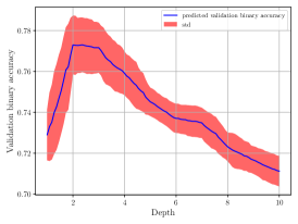
(a)

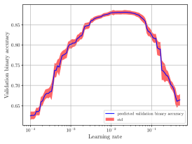
(b)

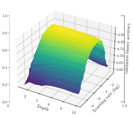
(c)

Figure 1: Examples of marginals for a quantum neural network with validation accuracy as performance on the banknote-authentication dataset. The hyperparameters correspond to the learning rate used during training (a), and the number of layers, also known as depth (b), and their combination (c). The hyperparameter values for learning rate are on a log scale. When considered individually, we see for instance that depth and learning rate should not be set too high for better performances. However, when grouped together, the learning rate seems most influential.

2.2 Supervised learning with Parameterized Quantum Circuits

2.2.1 Basics of quantum computing

In quantum computing, computations are carried out by the manipulation of qubits, similarly to classical computing with bits. A system of $n$ qubits is represented by a $2^{n}$-dimensional complex vector in the Hilbert space $\mathcal{H}=(\mathbb{C}^{2})^{\otimes n}$. This vector describes the state of the system $\ket{\psi}\in\mathcal{H}$ of unit norm $\innerproduct{\psi}{\psi}=1$. The bra-ket notation is used to describe vectors $\ket{\psi}$, their conjugate transpose $\bra{\psi}$ and inner-products $\innerproduct{\psi}{\psi^{\prime}}$ in $\mathcal{H}$. Single-qubit computational basis states are given by $\ket{0}=(1,0)^{T},\ket{1}=(0,1)^{T}$, and their tensor products describe general computational basis states, e.g., $\ket{10}=\ket{1}\otimes\ket{0}=(0,0,1,0)$.

The quantum state is modified with unitary operations or gates $U$ acting on $\mathcal{H}$. This computation can be represented by a quantum circuit (see Fig. 2). When a gate $U$ acts non-trivially only on a subset $S\subseteq[n]$ of qubits, we denote such operation $U\otimes\mathbbm{1}_{\_}{[n]\backslash S}$. In this work, we use, the Hadamard gate $H$, the single-qubit Pauli gates $Z,Y$ and their associated rotations $R_{\_}X,R_{\_}Y,R_{\_}Z$:

$$\begin{gathered}H=\frac{1}{\sqrt{2}}\begin{pmatrix}1&1\\ 1&-1\end{pmatrix},Z=\begin{pmatrix}1&0\\ 0&-1\end{pmatrix},R_{\_}Z(w)=\exp(-i\frac{w}{2}Z),\\ Y=\begin{pmatrix}0&-i\\ i&0\end{pmatrix},R_{\_}Y(w)=\exp(-i\frac{w}{2}Y),X=\begin{pmatrix}0&1\\ 1&0\end{pmatrix},R_{\_}X(w)=\exp(-i\frac{w}{2}X),\end{gathered}$$ (1)

The rotation angles are denoted $w\in\mathbb{R}$ and the 2-qubit controlled-$Z$ gate $\leavevmode\hbox to2.5pt{\vbox to8.96pt{\text{[drawing]}}}=\text{diag}(1,1,1,-1)$ as well as the $\sqrt{\text{iSWAP}}$ given by the matrix

$$\frac{1}{\sqrt{2}}\begin{pmatrix}\sqrt{2}&0&0&0\\ 0&1&i&0\\ 0&i&1&0\\ 0&0&0&\sqrt{2}\end{pmatrix}.$$ (2)

Measurements are carried out at the end of a quantum circuit to obtain bitstrings. Such measurement operation is described by a Hermitian operator $O$ called an observable. Its spectral decomposition $O=\sum_{\_}m\lambda_{\_}mP_{\_}m$ in terms of eigenvalues $\lambda_{\_}m$ and orthogonal projections $P_{\_}m$ defines the outcomes of this measurement, according to the Born rule: a measured state $\ket{\psi}$ gives the outcome $\lambda_{\_}m$ and gets projected onto the state $P_{\_}m\ket{\psi}/\!\ \sqrt{p(m})$ with probability $p(m)=\bra{\psi}P_{\_}m\ket{\psi}=\expectationvalue{P_{\_}m}_{\_}\psi$. The expectation value of the observable $O$ with respect to $\ket{\psi}$ is $\mathbb{E}_{\_}\psi[O]=\sum_{\_}mp(m)\lambda_{\_}m=\expectationvalue{O}_{\_}{\psi}$. We refer to [30] for more basic concepts of quantum computing, and follow with parameterized quantum circuits.

2.2.2 Parameterized Quantum Circuits

A parameterized quantum circuit (also called ansatz) can be represented by a quantum circuit with adjustable real-valued parameters $\bm{\theta}$. The latter is then defined by a unitary $U(\bm{\theta})$ that acts on a fixed $n$-qubit state (e.g., $\ket{0^{\otimes n}}$). The ansatz may be constructed using the formulation of the problem at hand (typically the case in chemistry [27] or optimization [10]), or with a problem-independent generic construction. The latter are often designated as hardware-efficient.

For a machine learning task, this unitary encodes an input data instance $x\in\mathbb{R}^{d}$ and is parameterized by a trainable vector $\bm{\theta}$. Many designs exist but hardware-efficient parameterized quantum circuits [19] with an alternating-layered architecture are often considered in quantum machine learning when no information on the structure of the data is provided. This architecture is depicted in an example presented in Fig. 2 and essentially consists of an alternation of encoding unitaries $U_{\_}\text{enc}$ and variational unitaries $U_{\_}\text{var}$. In the example, $U_{\_}\text{enc}$ is composed of single-qubit rotations $R_{\_}X$, and $U_{\_}\text{var}$ of single-qubit rotations $R_{\_}z,R_{\_}y$ and entangling Ctrl-$Z$ gates, represented as in Fig. 2, forming the entangling part of the circuit. Such entangling part denoted $U_{\_}\text{ent}$, can be defined by connectivity between qubits.

These parameterized quantum circuits are similar to neural networks where the circuit architecture is fixed and the gate parameters are adjusted by a classical optimizer such as gradient descent. They have also been named quantum neural networks. The parameterized layer can be repeated multiple times, which increases its expressive power like neural networks [43]. The data encoding strategy (such as reusing the encoding layer multiple times in the circuit - a strategy called data reuploading) also influences the latter [31, 40].

Finally, the user can define the observable(s) and the post-processing method to convert the circuit outputs into a prediction in the case of supervised learning. Commonly, observables based on the single-qubit $Z$ operator are used. When applied on $m\leq n$ qubits, the observable is represented by a $2^{m}-1$ square diagonal matrix with $\{-1,1\}$ values, and is denoted $\mathcal{O}=Z\otimes Z\otimes\cdots\otimes Z$.

Having introduced parameterized quantum circuits, we present the hyperparameters of the models, the configuration space, and the experimental setup for our functional ANOVA-based hyperparameter importance study.

Figure 2: Parameterized quantum circuit architecture example with $4$ qubits and ring connectivity (qubit $1$ is connected to $2$, $2$ to $3$, $3$ to $4$, and $4$ to $1$ makes a ring). The first layer of $R_{\_}X$ is the encoding layer $U_{\_}\text{enc}$, taking a data instance $x\in\mathbb{R}^{4}$ as input. It is followed by the entangling part with Ctrl-$Z$ gates. Finally a variational layer $U_{\_}\text{var}$ is applied. Eventually, we do measurements to be converted into predictions for a supervised task. The dashed part can be repeated many times to increase the expressive power of the model.

3 Methods

In this section, we describe the network type and its hyperparameters and define the methodology that we follow.

3.1 Hyperparameters and configuration space

Many designs have been proposed for parameterized quantum circuits depending on the problem at hand or motivated research questions and contributions. Such propositions can be aggregated and translated into a set of hyperparameters and configuration space for the importance study. As such, we first did an extensive literature review on parameterized quantum circuits for machine learning [2, 14, 15, 17, 18, 21, 23, 24, 25, 32, 38, 44, 47, 48, 49, 50] as well as quantum machine learning software [1, 3, 7]. This resulted in a list of $10$ hyperparameters, presented in Table 1. We choose them so we balance between having well-known hyperparameters that are expected to be important, and less considered ones in the literature. For instance, many works use Adam [20] as the underlying optimizer, and the learning rate should generally be well chosen. On the contrary, the entangling gate used in the parameterized quantum circuit is generally a fixed choice.

From the literature, we expect data encoding strategy/circuit to be important. We choose two main forms for $U_{\_}\text{enc}$. The first one is the hardware-efficient $\bigotimes_{\_}{i=1}^{n}R_{\_}X(x_{\_}i)$. The second takes the following form from [3, 17, 14]:

$$U_{\_}\text{enc}(\bm{x})=U_{\_}z(\bm{x})H^{\otimes n}$$ (3)

$$U_{\_}z(\bm{x})=\exp(-\mathrm{i}\pi\left[\sum_{\_}{i=1}^{n}x_{\_}iZ_{\_}i+\sum_{\_}{\begin{subarray}{c}j=1,\\ j>i\end{subarray}}^{n}x_{\_}ix_{\_}jZ_{\_}iZ_{\_}j\right]).$$ (4)

Using data-reuploading [31] results in a more expressive model [40], and this was also demonstrated numerically [18, 31, 44]. Finally, pre-processing of the input is also sometimes used in encoding strategies that directly feed input features into Pauli rotations. It also influences the expressive power of the model [40]. In this work, we choose a usual activation function $tanh$ commonly used in neural networks. We do so as its range is $[-1,1]$, which is the same as the data features during training after the normalization step.

The list of hyperparameters we take into account is non-exhaustive. It can be extended at will, at the cost of more software engineering and budget for running experiments.

Table 1: List of hyperparameters considered for hyperparameter importance for quantum neural network, as we named them in our Tensorflow-Quantum code.

Hyperparameter	Values	Description
Adam learning rate	$[10^{-4},0.5]$ (log)	The learning rate with which the quantum neural network starts training. The range was taken from the automated machine learning library Auto-sklearn [11]. We uniformly sample taking the logarithmic scale.
batchsize	$16$, $32$, $64$	Number of samples in one batch of Adam used during training
depth	$\{1,2,$ $\cdots,10\}$	Number of variational layers defining the circuit
is dataencoding hardware efficient	True, False	Whether we use the hardware-efficient circuit $\bigotimes_{\_}{i=1}^{n}R_{\_}X(x_{\_}i)$ or an IQP circuit defined in Eq.3 to encode the input data.
use reuploading	True, False	Whether the data encoding layer is used before each variational layer or not.
have less rotations	True, False	If True, only use layers of $R_{\_}Y,R_{\_}Z$ gates as the variational layer. If False, add a layer of $R_{\_}X$ gates.
entangler operation	cz, sqiswap	Which entangling gate to use in $U_{\_}\text{ent}$
map type	ring, full, pairs	The connectivity used for $U_{\_}\text{ent}$. The ring connectivity use an entangling gate between consecutive indices $(i,i+1),i\in\{1,\dots,n\}$ of qubits. The full one uses a gate between each pair of indices $(i,j),i<j$. Pairs connects even consecutive indices first, then odd consecutive ones.
input activation function	linear, tanh	Whether to input $tanh(x_{\_}i)$ as rotations or just $x_{\_}i$.
output circuit	2Z, mZ	The observable(s) used as output(s) of the circuit. If 2Z, we use all possible pairs of qubit indices defining $Z\otimes Z$. If mZ, the tensor product acts on all qubits. Note we do not use single-qubit $Z$ observables although they are quite often used in the literature. Indeed, they are provably not using the entire circuit when it is shallow. Hence we decided to use $Z\otimes Z$ instead. Also, a single neuron layer with a sigmoid activation function is used as a final decision layer similar to [38].

3.2 Assessing Hyperparameter Importance

Once the list of hyperparameters and configuration space are decided, we perform the hyperparameter importance analysis with the functional ANOVA framework. Assessing the importance of the hyperparameters boils down to four steps. Firstly, the models are applied to various datasets by sampling various configurations in a hyperparameter optimization process. The performances or metrics of the models are recorded along. The sampled configurations and performances serve as data for functional ANOVA. As functional ANOVA uses internally tree-based surrogate models, namely random forests [6], we decided to add an extra step with reference to [34]. As the second step, we verify the performance of the internal surrogate models. We cross-evaluate them using regression metrics commonly used in surrogate benchmarks [9]. Surrogates performing badly at this step are then discarded from the importance analysis, as they can deteriorate the quality of the study. Thirdly, the marginal contribution of each hyperparameter over all datasets can be then obtained and used to infer a ranking of their importance. Finally, a verification step similar to [34] is carried out to confirm the inferred ranking previously obtained. We explain such a procedure in the following section.

3.3 Verifying Hyperparameter Importance

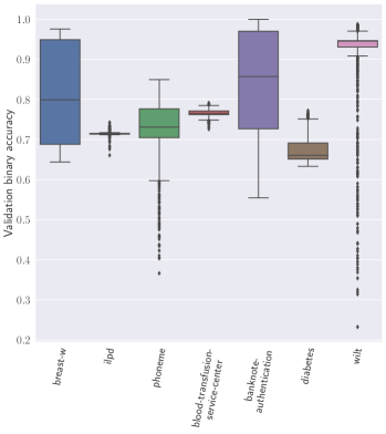
Figure 3: Performances of $1\,000$ quantim machine learning models defined by different configurations of hyperparameters over each dataset. The metric of interest in the study is the $10$-fold cross-validation accuracy. We take the best-achieved metric per model trained over $100$ epochs.

When applying the functional ANOVA framework, an extra verification step is added to confirm the output from a more intuitive notion of hyperparameter importance [34]. It is based on the assumption that hyperparameters that perform badly when fixed to a certain value (while other hyperparameters are optimized), will be important to optimize. The authors of [34] proposed to carry out a costly random search procedure fixing one hyperparameter at a time. In order to avoud a bias to the chosen value to which this hyperparameter is fixed, several values are chosen, and the optimization procedure is carried out multiple times. Formally, for each hyperparameter $\theta_{\_}j$ we measure $y^{*}_{\_}{j,f}$ as the result of a random search for maximizing the metric, fixing $\theta_{\_}j$ to a given value $f\in F_{\_}j,F_{\_}j\subseteq\Theta_{\_}j$. For categorical $\theta_{\_}j$ with domain $\Theta_{\_}j$, $F_{\_}j=\Theta_{\_}j$ is used. For numeric $\theta_{\_}j$, the authors of [34] use a set of $10$ values spread uniformly over $\theta_{\_}j$’s range. We then compute $y^{*}_{\_}j=\frac{1}{|F_{\_}j|}\sum_{\_}{f\in F_{\_}j}y^{*}_{\_}{j,f}$, representing the score when not optimizing hyperparameter $\theta_{\_}j$, averaged over fixing $\theta_{\_}j$ to various values it can take. Hyperparameters with lower value for $y^{*}_{\_}j$ are assumed to be more important, since the performance should deteriorate more when set sub-optimally.

In our study, we extend this framework to be used on the scale of quantum machine learning models. As quantum simulations can be very expensive, we carry out the verification experiment by using the predictions of the surrogate instead of fitting new quantum models during the verification experiment. The surrogates yield predictions $\hat{y}$ for the performance of arbitrary hyperparameter settings sampled during a random search. Hence, they serve to compute $y^{*}_{\_}{j,f}$. This is also why we assessed the quality of the built-in surrogates as the second step. Poorly-performing surrogates can deteriorate the quality of the random search procedure.

4 Dataset and inclusion criteria

To apply our quantum models and study the importance of the previously introduced hyperparameters, we consider classical datasets. Similarly to [34], we use datasets from the OpenML-CC18 benchmark suite [4]. In our study, we consider only the case where the number of qubits available is equal to the number of features, a common setting in the quantum community. As simulating quantum circuits is a costly task, we limit this study to the case where the number of features is less than $20$ after preprocessing. Our first step was to identify which datasets fit this criterion. We include all datasets from the OpenML-CC18 that have 20 or fewer features after categorical hyperparameters have been one-hot-encoded, and constant features are removed. Afterward, the input variables are also scaled to unit variance as a normalization step. The scaling constants are calculated on the training data and applied to the test data.

The final list of datasets is given in Table 2. In total, $7$ datasets fitted the criterion considered in this study. For all of them, we picked the OpenML Task ID giving the $10$-fold cross-validation task. A quantum model is then applied using the latter procedure, with the aforementioned preprocessing steps.

Table 2: List of datasets used in this study. The number of features is obtained after a usual preprocessing used in machine learning methods, such as one-hot-encoding.

Dataset	OpenML Task ID	Number of features	Number of instances
breast-w	15	$9$	$699$
diabetes	37	$8$	$768$
phoneme	9952	$5$	$5\,404$
ilpd	9971	$11$	$583$
banknote-authentication	10093	$4$	$1\,372$
blood-transfusion-service-center	10 101	$4$	$748$
wilt	146820	$5$	$4\,839$

5 Results

In this section, we present the results obtained using the hyperparameters and the methodology defined in Section 3 with the datasets described in Section 4. First, we show the distribution of performances obtained during a random search where configurations are independently sampled for each dataset. Then we carry out the surrogate verification. Finally, we present the functional ANOVA results in terms of hyperparameter importance with marginal contributions and the random search verification per hyperparameter.

5.1 Performance distributions per dataset

For each dataset, we sampled independently $1\,000$ hyperparameter configurations and run the quantum models for $100$ epochs as budget. As a performance measure, we recorded the best validation accuracy obtained over $100$ epochs. Fig. 3 shows the distribution of the $10$-fold cross-validation accuracy obtained per dataset. We observe the impact of hyperparameter optimization by the difference between the least performing and the best model configuration. For instance, on the wilt dataset, the best model gets an accuracy close to $1$, and the least below $0.25$. We can also see that some datasets present a smaller spread of performances. ilpd and blood-transfusion-service-center are in this case. It seems that hyperparameter optimization does not have a real effect, because most hyperparameter configurations give the same result. As such, the surrogates could not differentiate between various configurations. In general, hyperparameter optimization is important for getting high performances per dataset and detecting datasets where the importance study can be applied.

5.2 Surrogate verification

Functional ANOVA relies on an internal surrogate model to determine the marginal contribution per hyperparameter. If this surrogate model is not accurate, this can have a severe limitation on the conclusions drawn from functional ANOVA. In this experiment, we verify whether the hyperparameters can explain the performances of the models. Table 3 shows the performance of the internal surrogate models. We notice low regression scores for the two datasets (less than $0.75$ R2 scores). Hence we remove them from the analysis.

Table 3: Performances of the surrogate models built within functional ANOVA over a $10$-fold cross-validation procedure. We present the average coefficient of determination (R2), root mean squared error (RMSE), and Spearman’s rank correlation coefficient (CC). These are common regression metrics for benchmarking surrogate models on hyperparameters [9]. The surrogates over ilpd and blood-transfusion-service-center obtain low scores (less than $.75$ R2), hence we remove them from the study.

Dataset	R2 score	RMSE	CC
breast-w	0.8663	0.0436	0.9299
diabetes	0.7839	0.0155	0.8456
phoneme	0.8649	0.0285	0.9282
ilpd	0.1939	0.0040	0.4530
banknote-authentication	0.8579	0.0507	0.9399
blood-transfusion-service-center	0.6104	0.0056	0.8088
wilt	0.7912	0.0515	0.8015

5.3 Marginal contributions

For functional ANOVA, we used $128$ trees for the surrogate model. Fig. 4(a,b) shows the marginal contribution of each hyperparameter over the remaining $5$ datasets. We distinguish $3$ main levels of importance. According to these results, the learning rate, depth, and the data encoding circuit and reuploading strategy are critical. These results are in line with our expectations. The entangler gate, connectivity, and whether we use $R_{\_}X$ gates in the variational layer are the least important according to functional ANOVA. Hence, our results reveal new insights into these hyperparameters that are not considered in general.

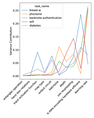
(a)

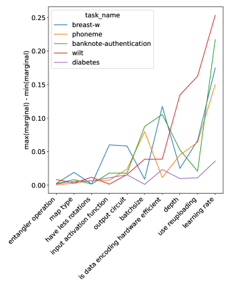
(b)

Figure 4: The marginal contributions per dataset are presented as a) the variance contribution and b) the difference between the minimal and maximal value of the marginal of each hyperparameter. The hyperparameters are sorted from the least to most important using the median. We distinguish from the plot $3$ main levels of importance.

5.4 Random search verification

In line with the work of [34], we perform an additional verification experiment that verifies whether the outcomes of functional ANOVA are in line with our expectations. However, the verification procedure involves an expensive, post-hoc analysis: a random search procedure fixing one hyperparameter at a time. As our quantum simulations are costly, we used the surrogate models fitted on the current dataset considered over the $1\,000$ configurations obtained initially to predict the performances one would obtain when presented with a new configuration.

Fig. 5 shows the average rank of each run of random search, labeled with the hyperparameter whose value was fixed to a default value. A high rank implies poor performance compared to the other configurations, meaning that tuning this hyperparameter would have been important. We witness again the $3$ levels of importance, with almost the same order obtained. However, the input_activation_function is deemed more important while batchsize is less.

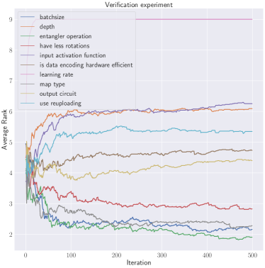
Figure 5: Verification experiment of the importance of the hyperparameters. A random search procedure up to $500$ iterations excluding one parameter at a time is used. A lower curve means the hyperparameter is deemed less important.

More simulations with more datasets may be required to validate the importance. However, we retrieve empirically the importance of well-known hyperparameters while considering less important ones. Hence functional ANOVA becomes an interesting tool for quantum machine learning in practice.

6 Conclusion

In this work, we study the importance of hyperparameters related to quantum neural networks for classification using the functional ANOVA framework. Our experiments are carried out over OpenML datasets that match the current scale of quantum hardware simulations (i.e., datasets that have at most $20$ features after pre-processing operators have been applied, hence using $20$ qubits). We selected and presented the hyperparameters from an aggregation of quantum computing literature and software. Firstly, hyperparameter optimization highlighted datasets where we observed high differences between configurations. This underlines the importance of hyperparameter optimization for these datasets. There were also datasets that showed little difference. These led us to extend the methodology by adding an additional verification step of the internal surrogate performances. From our results, we distinguished $3$ main levels of importance. On the one hand, Adam’s learning rate, depth, and the data encoding strategy are deemed very important, as we expected. On the other hand, the less considered hyperparameters such as the particular choice of the entangling gate and using $3$ rotation types in the variational layer are in the least important group. Hence, our experiment both confirmed expected patterns and revealed new insights for quantum model selection.

For future work, we plan to further investigate methods from the field of automated machine learning to be applied to quantum neural networks [5, 26, 11]. Indeed, our experiments have shown the importance of hyperparameter optimization, and this should become standard practice and part of the protocols applied within the community. We further envision functional ANOVA to be employed in future works related to quantum machine learning and understanding how to apply quantum models in practice. For instance, it would be interesting to consider quantum data, for which quantum machine learning models may have an advantage. Plus, extending hyperparameter importance to techniques for scaling to a large number of features with the number of qubits, such as dimensionality reduction or divide-and-conquer techniques, can be left for future work. Finally, this type of study can also be extended to different noisy hardware and towards algorithm/model selection and design. If we have access to a cluster of different quantum computers, then choosing which hardware works best for machine learning tasks becomes possible. One could also extend our work with meta-learning [5], where a model configuration is selected based on meta-features created from dataset features. Such types of studies already exist for parameterized quantum circuits applied to combinatorial optimization [28, 29, 37].

Acknowledgements CM and VD acknowledge support from TotalEnergies. This work was supported by the Dutch Research Council (NWO/OCW), as part of the Quantum Software Consortium programme (project number 024.003.037). This research is also supported by the project NEASQC funded from the European Union’s Horizon 2020 research and innovation programme (grant agreement No 951821).

References

- [1] ANIS, M.S., et al.: Qiskit: An open-source framework for quantum computing (2021). https://doi.org/10.5281/zenodo.2573505
- [2] Benedetti, M., Lloyd, E., Sack, S., Fiorentini, M.: Parameterized quantum circuits as machine learning models. Quantum Science and Technology 4(4), 043001 (2019)
- [3] Bergholm, V., Izaac, J.A., Schuld, M., Gogolin, C., Killoran, N.: Pennylane: Automatic differentiation of hybrid quantum-classical computations. CoRR abs/1811.04968 (2018)
- [4] Bischl, B., Casalicchio, G., Feurer, M., Gijsbers, P., Hutter, F., Lang, M., Mantovani, R.G., van Rijn, J.N., Vanschoren, J.: Openml benchmarking suites. In: Proceedings of the Neural Information Processing Systems Track on Datasets and Benchmarks (2021)
- [5] Brazdil, P., van Rijn, J.N., Soares, C., Vanschoren, J.: Metalearning: Applications to Automated Machine Learning and Data Mining. Springer, 2nd edn. (2022)
- [6] Breiman, L.: Random forests. Machine Learning 45(1), 5–32 (2001)
- [7] Broughton, M., et al.: Tensorflow quantum: A software framework for quantum machine learning. arXiv:2003.02989 (2020)
- [8] Caro, M.C., Gil-Fuster, E., Meyer, J.J., Eisert, J., Sweke, R.: Encoding-dependent generalization bounds for parametrized quantum circuits. Quantum 5, 582 (2021)
- [9] Eggensperger, K., Hutter, F., Hoos, H.H., Leyton-Brown, K.: Efficient benchmarking of hyperparameter optimizers via surrogates. In: Proceedings of the Twenty-Ninth AAAI Conference on Artificial Intelligence. pp. 1114–1120. AAAI Press (2015)
- [10] Farhi, E., Goldstone, J., Gutmann, S.: A quantum approximate optimization algorithm. arXiv:1411.4028 (2014)
- [11] Feurer, M., Eggensperger, K., Falkner, S., Lindauer, M., Hutter, F.: Auto-sklearn 2.0: Hands-free automl via meta-learning. arXiv:2007.04074v2 [cs.LG] (2021)
- [12] Georgescu, I.M., Ashhab, S., Nori, F.: Quantum simulation. Review of Modern Physics 86, 153–185 (2014)
- [13] Haug, T., Self, C.N., Kim, M.S.: Large-scale quantum machine learning. CoRR abs/2108.01039 (2021)
- [14] Havlíček, V., Córcoles, A.D., Temme, K., Harrow, A.W., Kandala, A., Chow, J.M., Gambetta, J.M.: Supervised learning with quantum-enhanced feature spaces. Nature 567(7747), 209–212 (2019)
- [15] Heimann, D., Hohenfeld, H., Wiebe, F., Kirchner, F.: Quantum deep reinforcement learning for robot navigation tasks. CoRR abs/2202.12180 (2022)
- [16] Hutter, F., Hoos, H., Leyton-Brown, K.: An efficient approach for assessing hyperparameter importance. In: Proceedings of the 31th International Conference on Machine Learning, ICML 2014. JMLR Workshop and Conference Proceedings, vol. 32, pp. 1130–1144 (2014)
- [17] Jerbi, S., Fiderer, L.J., Nautrup, H.P., Kübler, J.M., Briegel, H.J., Dunjko, V.: Quantum machine learning beyond kernel methods. CoRR abs/2110.13162 (2021)
- [18] Jerbi, S., Gyurik, C., Marshall, S., Briegel, H.J., Dunjko, V.: Parametrized quantum policies for reinforcement learning. In: Advances in Neural Information Processing Systems 34. pp. 28362–28375 (2021)
- [19] Kandala, A., Mezzacapo, A., Temme, K., Takita, M., Brink, M., Chow, J.M., Gambetta, J.M.: Hardware-efficient variational quantum eigensolver for small molecules and quantum magnets. Nature 549(7671), 242–246 (2017)
- [20] Kingma, D.P., Ba, J.: Adam: A method for stochastic optimization (2015)
- [21] Liu, J.G., Wang, L.: Differentiable learning of quantum circuit born machines. Physical Review A 98, 062324 (2018)
- [22] Liu, Y., Arunachalam, S., Temme, K.: A rigorous and robust quantum speed-up in supervised machine learning. Nature Physics 17(9), 1013–1017 (2021)
- [23] Marshall, S.C., Gyurik, C., Dunjko, V.: High dimensional quantum machine learning with small quantum computers. CoRR abs/2203.13739 (2022)
- [24] Mensa, S., Sahin, E., Tacchino, F., Barkoutsos, P.K., Tavernelli, I.: Quantum machine learning framework for virtual screening in drug discovery: a prospective quantum advantage. CoRR abs/2204.04017 (2022)
- [25] Mitarai, K., Negoro, M., Kitagawa, M., Fujii, K.: Quantum circuit learning. Physical Review A 98, 032309 (2018)
- [26] Mohr, F., van Rijn, J.N.: Learning curves for decision making in supervised machine learning - A survey. CoRR abs/2201.12150 (2022)
- [27] Moll, N., et al: Quantum optimization using variational algorithms on near-term quantum devices. Quantum Science and Technology 3(3), 030503 (2018)
- [28] Moussa, C., Calandra, H., Dunjko, V.: To quantum or not to quantum: towards algorithm selection in near-term quantum optimization. Quantum Science and Technology 5(4), 044009 (2020)
- [29] Moussa, C., Wang, H., Bäck, T., Dunjko, V.: Unsupervised strategies for identifying optimal parameters in quantum approximate optimization algorithm. EPJ Quantum Technology 9(1) (2022)
- [30] Nielsen, M.A., Chuang, I.L.: Quantum Computation and Quantum Information: 10th Anniversary Edition. Cambridge University Press (2011)
- [31] Pérez-Salinas, A., Cervera-Lierta, A., Gil-Fuster, E., Latorre, J.I.: Data re-uploading for a universal quantum classifier. Quantum 4, 226 (2020)
- [32] Peters, E., Caldeira, J., Ho, A., Leichenauer, S., Mohseni, M., Neven, H., Spentzouris, P., Strain, D., Perdue, G.N.: Machine learning of high dimensional data on a noisy quantum processor. npj Quantum Information 7(1), 161 (2021)
- [33] Preskill, J.: Quantum Computing in the NISQ era and beyond. Quantum 2, 79 (2018)
- [34] van Rijn, J.N., Hutter, F.: Hyperparameter importance across datasets. In: Proceedings of the 24th ACM SIGKDD International Conference on Knowledge Discovery & Data Mining, KDD 2018. pp. 2367–2376. ACM (2018)
- [35] Sajjan, M., Li, J., Selvarajan, R., Sureshbabu, S.H., Kale, S.S., Gupta, R., Kais, S.: Quantum computing enhanced machine learning for physico-chemical applications. CoRR arXiv:2111.00851 (2021)
- [36] Saltelli, A., Sobol, I.: Sensitivity analysis for nonlinear mathematical models: Numerical experience. Matematicheskoe Modelirovanie 7 (1995)
- [37] Sauvage, F., Sim, S., Kunitsa, A.A., Simon, W.A., Mauri, M., Perdomo-Ortiz, A.: Flip: A flexible initializer for arbitrarily-sized parametrized quantum circuits. CoRR abs/2103.08572 (2021)
- [38] Schetakis, N., Aghamalyan, D., Boguslavsky, M., Griffin, P.: Binary classifiers for noisy datasets: a comparative study of existing quantum machine learning frameworks and some new approaches. CoRR abs/2111.03372 (2021)
- [39] Schuld, M., Killoran, N.: Is quantum advantage the right goal for quantum machine learning? Corr abs/2203.01340 (2022)
- [40] Schuld, M., Sweke, R., Meyer, J.J.: Effect of data encoding on the expressive power of variational quantum-machine-learning models. Physical Review A 103, 032430 (2021)
- [41] Sharma, A., van Rijn, J.N., Hutter, F., Müller, A.: Hyperparameter importance for image classification by residual neural networks. In: Discovery Science - 22nd International Conference. Lecture Notes in Computer Science, vol. 11828, pp. 112–126. Springer (2019)
- [42] Shor, P.W.: Polynomial-time algorithms for prime factorization and discrete logarithms on a quantum computer. Siam Review 41, 303–332 (1999)
- [43] Sim, S., Johnson, P.D., Aspuru-Guzik, A.: Expressibility and entangling capability of parameterized quantum circuits for hybrid quantum-classical algorithms. Advanced Quantum Technologies 2(12), 1900070 (2019)
- [44] Skolik, A., Jerbi, S., Dunjko, V.: Quantum agents in the gym: a variational quantum algorithm for deep q-learning. CoRR abs/2103.15084 (2021)
- [45] Sobol, I.M.: Sensitivity estimates for nonlinear mathematical models. Mathematical Modelling and Computational Experiments 1(4), 407–414 (1993)
- [46] Sweke, R., Seifert, J., Hangleiter, D., Eisert, J.: On the quantum versus classical learnability of discrete distributions. Quantum 5, 417 (2021)
- [47] Wang, H., Gu, J., Ding, Y., Li, Z., Chong, F.T., Pan, D.Z., Han, S.: Quantumnat: Quantum noise-aware training with noise injection, quantization and normalization. CoRR abs/2110.11331 (2021)
- [48] Wang, H., Li, Z., Gu, J., Ding, Y., Pan, D.Z., Han, S.: Qoc: Quantum on-chip training with parameter shift and gradient pruning. CoRR abs/2202.13239 (2022)
- [49] Wossnig, L.: Quantum machine learning for classical data. CoRR abs/2105.03684 (2021)
- [50] Zoufal, C., Lucchi, A., Woerner, S.: Quantum generative adversarial networks for learning and loading random distributions. npj Quantum Information 5(1), 103 (2019)