Thompson Sampling Efficiently Learns to Control Diffusion Processes

Abstract

Diffusion processes that evolve according to linear stochastic differential equations are an important family of continuous-time dynamic decision-making models. Optimal policies are well-studied for them, under full certainty about the drift matrices. However, little is known about data-driven control of diffusion processes with uncertain drift matrices as conventional discrete-time analysis techniques are not applicable. In addition, while the task can be viewed as a reinforcement learning problem involving exploration and exploitation trade-off, ensuring system stability is a fundamental component of designing optimal policies. We establish that the popular Thompson sampling algorithm learns optimal actions fast, incurring only a square-root of time regret, and also stabilizes the system in a short time period. To the best of our knowledge, this is the first such result for Thompson sampling in a diffusion process control problem. We validate our theoretical results through empirical simulations with real parameter matrices from two settings of airplane and blood glucose control. Moreover, we observe that Thompson sampling significantly improves (worst-case) regret, compared to the state-of-the-art algorithms, suggesting Thompson sampling explores in a more guarded fashion. Our theoretical analysis involves characterization of a certain optimality manifold that ties the local geometry of the drift parameters to the optimal control of the diffusion process. We expect this technique to be of broader interest.

1 Introduction

One of the most natural reinforcement learning (RL) algorithms for controlling a diffusion process with unknown parameters is based on Thompson sampling (TS) [1]: a Bayesian posterior for the model is calculated based on its time evolution, and a control policy is then designed by treating a sampled model from the posterior as the truth. Despite its simplicity, guaranteeing efficiency and whether sampling the actions from the posterior could lead to unbounded future trajectories is unknown. In fact, the only known such theoretical result for control of a diffusion process is for an epsilon-greedy type policy that requires selecting purely random actions at a certain rate [2].

In this work, we consider a $p$ dimensional state signal $\left\{\boldsymbol{x}_{t}\right\}_{t\geq 0}$ that obeys the (Ito) stochastic differential equation (SDE)

$$\boldsymbol{d}\boldsymbol{x}_{t}=\left(A_{0}\boldsymbol{x}_{t}+B_{0}\boldsymbol{u}_{t}\right)\boldsymbol{d}t+\boldsymbol{d}\mathbb{W}_{t}\,,$$ (1)

where the drift matrices $A_{0}$ and $B_{0}$ are unknown, $\boldsymbol{u}_{t}\in\mathbb{R}^{q}$ is the control action at any time $t\geq 0$, and it is designed based on values of $\boldsymbol{x}_{s}$ for $s\in[0,t]$. The matrix $B_{0}\in\mathbb{R}^{p\times q}$ models the influence of the control action on the state evolution over time, while $A_{0}\in\mathbb{R}^{p\times p}$ is the (open-loop) transition matrix reflecting interactions between the coordinates of the state vector $\boldsymbol{x}_{t}$. The diffusion term in (1) consists of a non-standard Wiener process $\mathbb{W}_{t}$ that will be defined in the next section. The goal is to study efficient RL policies that can design $\boldsymbol{u}_{t}$ to minimize a quadratic cost function, defined in the next section, subject to uncertainties around $A_{0}$ and $B_{0}$.

At a first glance, this problem is similar to most RL problems since the optimal policy must balance between the two objectives of learning the unknown matrices $A_{0}$ and $B_{0}$ (exploration) and optimally selecting the control signals $\boldsymbol{u}_{t}$ to minimize the cost (exploitation). However, unlike most RL problems that have finite or bounded-support state space, ensuring stability, that $\boldsymbol{x}_{t}$ stays bounded, is a crucial part of designing optimal policies. For example, in the discrete-time version of the problem, robust exploration is used to protect against unpredictably unstable trajectories [3, 4, 5, 6].

Related literature.

The existing literature studies efficiency of TS for learning optimal decisions in finite action spaces [7, 8, 9, 10, 11, 12]. In this stream of research, it is shown that, over time, the posterior distribution concentrates around low-cost actions [13, 14, 15]. TS is also studied in further discrete-time settings with the environment represented by parameters that belong to a continuum, and Bayesian and frequentist regret bounds are shown for linear-quadratic regulators [16, 17, 18, 19, 20, 21, 22, 23, 24]. However, effectiveness of TS in highly noisy environments that are modeled by diffusion processes remains unexplored to date, due to technical challenges that will be described below.

For continuous-time linear time invariant dynamical systems, infinite-time consistency results are shown under a variety of technical assumptions, followed by alternating policies that cause (small) linear regrets [25, 26, 27, 28, 29]. From a computational viewpoint, pure exploration algorithms for computing optimal policies based on multiple trajectories of the state and action data are studied as well [30, 31, 32], for which a useful survey is available [33]. However, papers that study exploration versus exploitation, and provide non-asymptotic estimation rates or regret bounds are limited to a few recent work about offline RL or stabilized processes [34, 2, 35, 36].

Contributions.

This work, first establishes that TS learns to stabilize the diffusion process (1). Specifically, in Theorem 1 of Section 3, we provide the first theoretical stabilization guarantee for diffusion processes, showing that the probability of preventing the state process from growing unbounded grows to 1, at an exponential rate that depends on square-root of the time length devoted to stabilization. As mentioned above, for RL problems with finite state spaces, the process is by definition stabilized, regardless of the policy. However, for the Euclidean state space of $\boldsymbol{x}_{t}$ in (1), stabilization is necessary to ensure that the state and the cost do not grow unbounded.

Then, efficiency of TS in balancing exploration versus exploitation for minimizing a cost function that has a quadratic form of both the state and the control action is shown. Indeed, we establish in Theorem 2 of Section 4 that the regret TS incurs, grows as the square-root of time, while the squared estimation error decays with the same rate. It is also shown that both the above quantities grow quadratically with the dimension. To the authors’ knowledge, the presented results are the first theoretical analyses of TS for learning to control diffusion processes.

Additionally, through extensive simulations we illustrate that TS enjoys smaller average regret and substantially lower worst-case regret than the existing RL policies, thanks to its informed exploration.

It is important to highlight that theoretical analysis of RL policies for diffusion processes is highly non-trivial. Specifically, the conventional discrete-time RL technical tools are not applicable, due to uncountable cardinality of the random variables involved in a diffusion process, the unavoidable dependence between them, and the high level of processing and estimation noise. To address these, we make four main contributions. First, non-asymptotic and uniform upper bounds for continuous-time martingales and for Ito integrals are required to quantify the estimation accuracy. For that purpose, we establish concentration inequalities and show sub-exponential tail bounds for double stochastic integrals. Second, one needs sharp bounds for the impact of estimation errors on eigenvalues of certain non-linear matrices of the drift parameters that determine actions taken by TS policy. To tackle that, we perform a novel and tight eigenvalue perturbation-analysis based on the approximation error, dimension, and spectrum of the matrices. We also establish Lipschitz continuity of the control policy with respect to the drift matrices, by developing new techniques based on matrix-valued curves. Third, to capture evaluation of both immediate and long-term effects of sub-optimal actions, we employ Ito calculus to bound the stochastic regret and specify effects of all problem parameters. Finally, to study learning from data trajectories that the condition number of their information matrix grows unbounded, we develop stochastic inequalities for self-normalized continuous-time martingales, and spectral analysis of non-linear functions of random matrices.

Organization.

The organization of the subsequent sections is as follows. We formulate the problem in Section 2, while Algorithm 1 that utilizes TS for learning to stabilize the process and its high-probability performance guarantee are presented in Section 3. Then, in Section 4, TS is considered for learning to minimize a quadratic cost function, and the rates of estimation and regret are established. Next, theoretical analysis are provided in Section 5, followed by real-world numerical results of Section 6. Detailed proofs and auxiliary lemmas are delegated to the appendices.

Notation.

The smallest (the largest) eigenvalue of matrix $M$, in magnitude, is denoted by $\underline{\lambda}\left(M\right)$ ($\overline{\lambda}\left(M\right)$). For a vector $a$, ${\left|\kern-1.50696pt\left|a\right|\kern-1.50696pt\right|}$ is the $\ell_{2}$ norm, and for a matrix $M$, ${\left|\kern-1.50696pt\left|M\right|\kern-1.50696pt\right|}$ is the operator norm that is the supremum of ${\left|\kern-1.50696pt\left|Ma\right|\kern-1.50696pt\right|}$ for $a$ on the unit sphere. $\boldsymbol{N}\left(\mu,\Sigma\right)$ is Gaussian distribution with mean $\mu$ and covariance $\Sigma$. If $\mu$ is a matrix (instead of vector), then $\boldsymbol{N}\left(\mu,\Sigma\right)$ denotes a distribution on matrices of the same dimension as $\mu$, such that all columns are independent and share the covariance matrix $\Sigma$. In this paper, transition matrices $A\in\mathbb{R}^{p\times p}$ together with input matrices $B\in\mathbb{R}^{p\times q}$ are jointly denoted by the $(p+q)\times p$ parameter matrix $\boldsymbol{\theta}=\left[A,B\right]^{\top}$. We employ $\vee$ ($\wedge$) for maximum (minimum). Finally, $a\lesssim b$ expresses that $a\leq\alpha_{0}b$, for some fixed constant $\alpha_{0}$.

2 Problem Statement

We study the problem of designing provably efficient reinforcement learning policies for minimizing a quadratic cost function in an uncertain linear diffusion process. To proceed, fix the complete probability space $(\Omega,\left\{\mathcal{F}_{t}\right\}_{t\geq 0},\mathbb{P})$, where $\Omega$ is the sample space, $\left\{\mathcal{F}_{t}\right\}_{t\geq 0}$ is a continuous-time filtration (i.e., increasing sigma-fields), and $\mathbb{P}$ is the probability measure defined on $\mathcal{F}_{\infty}$.

The state comprises the diffusion process $\boldsymbol{x}_{t}$ in  (1), where $\boldsymbol{\theta_{0}}=\left[A_{0},B_{0}\right]^{\top}\in\mathbb{R}^{\left(p+q\right)\times p}$ is the unknown drift parameter. The diffusion term in (1) follows infinitesimal variations of the $p$ dimensional Wiener process $\left\{\mathbb{W}_{t}\right\}_{t\geq 0}$. That is, $\left\{\mathbb{W}_{t}\right\}_{t\geq 0}$ is a multivariate Gaussian process with independent increments and with the stationary covariance matrix $\Sigma_{\mathbb{W}}$, such that for all $0\leq s_{1}\leq s_{2}\leq t_{1}\leq t_{2}$,

$$\begin{bmatrix}\mathbb{W}_{t_{2}}-\mathbb{W}_{t_{1}}\\ \mathbb{W}_{s_{2}}-\mathbb{W}_{s_{1}}\end{bmatrix}\sim\boldsymbol{N}\left(\begin{bmatrix}0_{p}\\ 0_{p}\end{bmatrix},\begin{bmatrix}(t_{2}-t_{1})\Sigma_{\mathbb{W}}&0_{p\times p}\\ 0_{p\times p}&(s_{2}-s_{1})\Sigma_{\mathbb{W}}\end{bmatrix}\right).$$ (2)

Existence, construction, continuity, and non-differentiability of Wiener processes are well-known [37]. It is standard to assume that $\Sigma_{\mathbb{W}}$ is positive definite, which is a common condition in learning-based control [33, 34, 2, 35] to ensure accurate estimation over time.

The RL policy designs the action $\left\{\boldsymbol{u}_{t}\right\}_{t\geq 0}$, based on the observed system state by the time, as well as the previously applied actions, to minimize the long-run average cost

$$\limsup\limits_{T\to\infty}\frac{1}{T}\int\limits_{0}^{T}{\left[\boldsymbol{x}_{t}^{\top},\boldsymbol{u}_{t}^{\top}\right]Q\begin{bmatrix}\boldsymbol{x}_{t}\\ \boldsymbol{u}_{t}\end{bmatrix}}\boldsymbol{d}{t},~{}~{}~{}~{}~{}\text{for}~{}~{}~{}~{}Q=\begin{bmatrix}Q_{x}&Q_{xu}\\ Q_{xu}^{\top}&Q_{u}\end{bmatrix}.$$ (3)

Above, the cost is determined by the positive definite matrix $Q$, where $Q_{x}\in\mathbb{R}^{p\times p}$, $Q_{u}\in\mathbb{R}^{q\times q}$, $Q_{xu}\in\mathbb{R}^{p\times q}$. In fact, $Q$ determines the weights of different coordinates of $\boldsymbol{x}_{t},\boldsymbol{u}_{t}$ in the cost function, so that the policy aims to make the states small, by deploying small actions. The cost matrix $Q$ is assumed known to the policy. Formally, the problem is to minimize (3) by the policy

$$\boldsymbol{u}_{t}=\boldsymbol{\widehat{\pi}}\left(Q,\left\{\boldsymbol{x}_{s}\right\}_{0\leq s\leq t},\left\{\boldsymbol{u}_{s}\right\}_{0\leq s<t}\right).$$ (4)

Without loss of generality, and for the ease of presentation, we follow the canonical formulation that sets $Q_{xu}=0$; one can simply convert the case $Q_{xu}\neq 0$ to the canonical form, by employing a rotation to $\boldsymbol{x}_{t},\boldsymbol{u}_{t}$ [38, 39, 40, 41]. It is well-known that if, hypothetically, the truth $\boldsymbol{\theta_{0}}$ was known, an optimal policy $\boldsymbol{\pi_{\mathrm{opt}}}$ could be explicitly found by solving the continuous-time algebraic Riccati equation. That is, for a generic drift matrix $\boldsymbol{\theta}=\left[A,B\right]^{\top}$, finding the symmetric $p\times p$ matrix ${P}\left(\boldsymbol{\theta}\right)$ that satisfies

$$A^{\top}{P}\left(\boldsymbol{\theta}\right)+{P}\left(\boldsymbol{\theta}\right)A-{P}\left(\boldsymbol{\theta}\right)BQ_{u}^{-1}B^{\top}{P}\left(\boldsymbol{\theta}\right)+Q_{x}=0.$$ (5)

This means, for the true parameter $\boldsymbol{\theta_{0}}=\left[A_{0},B_{0}\right]^{\top}$, we can let ${P}\left(\boldsymbol{\theta_{0}}\right)$ solve the above equation, and define the policy

$$\boldsymbol{\pi_{\mathrm{opt}}}:\>\>\>\>\>\boldsymbol{u}_{t}=-Q_{u}^{-1}B_{0}^{\top}{P}\left(\boldsymbol{\theta_{0}}\right)\boldsymbol{x}_{t},\>\>\>\forall t\geq 0.$$ (6)

It is known that the linear time-invariant policy $\boldsymbol{\pi_{\mathrm{opt}}}$ minimizes the average cost in (3) [38, 39, 40, 41].

Definition 1

The process in (1) is stabilizable, if all eigenvalues of $\overline{A}={A_{0}+B_{0}K}$ have negative real-parts, for a matrix $K$. Such $K,\overline{A}$ are called a stabilizer and the stable closed-loop matrix.

We assume that the process (1) with the drift parameter $\boldsymbol{\theta_{0}}$ is stabilizable. Therefore, ${P}\left(\boldsymbol{\theta_{0}}\right)$ exists, is unique, and can be computed using continuous-time Riccati differential equations similar to (5), except that the zero matrix on the right-hand side will be replaced by the derivative of ${P}\left(\boldsymbol{\theta}\right)$ [38, 39, 40, 41]. Furthermore, it is known that real-parts of all eigenvalues of $\overline{A}_{0}=A_{0}-B_{0}Q_{u}^{-1}B_{0}^{\top}{P}\left(\boldsymbol{\theta_{0}}\right)$ are negative, i.e., $\left|\overline{\lambda}\left(\exp\left(\overline{A}_{0}t\right)\right)\right|<1$, which means the matrix $\exp\left(\overline{A}_{0}t\right)$ decays exponentially fast as $t$ grows [38, 39, 40, 41]. In the sequel, we use (5) and refer to the solution ${P}\left(\boldsymbol{\theta}\right)$ for different stabilizable $\boldsymbol{\theta}$. More details about the above optimal feedback policy can be found in the aforementioned references.

In absence of exact knowledge of $\boldsymbol{\theta_{0}}$, a policy $\boldsymbol{\widehat{\pi}}$ collects data and leverages it to approximate $\boldsymbol{\pi_{\mathrm{opt}}}$ in (6). Therefore, at all (finite) times, there is a gap between the cost of $\boldsymbol{\widehat{\pi}}$, compared to that of $\boldsymbol{\pi_{\mathrm{opt}}}$. The cumulative performance degradation due to this gap is the regret of the policy $\boldsymbol{\widehat{\pi}}$, that we aim to minimize. Technically, whenever the control action $\boldsymbol{u}_{t}$ is designed by the policy $\boldsymbol{\widehat{\pi}}$ according to (4), concatenate the resulting state and input signals to get the observation $\boldsymbol{z}_{t}(\boldsymbol{\widehat{\pi}})=\left[\boldsymbol{x}_{t}^{\top},\boldsymbol{u}_{t}^{\top}\right]^{\top}$. If it is clear from the context, we drop $\boldsymbol{\widehat{\pi}}$. Similarly, $\boldsymbol{z}_{t}(\boldsymbol{\pi_{\mathrm{opt}}})$ denotes the observation signal of $\boldsymbol{\pi_{\mathrm{opt}}}$. Now, the regret at time $T$ is defined by:

$$\mathrm{Reg}_{\boldsymbol{\widehat{\pi}}}\left(T\right)=\int\limits_{0}^{T}{\left({\left|\kern-1.50696pt\left|Q^{1/2}\boldsymbol{z}_{t}(\boldsymbol{\widehat{\pi}})\right|\kern-1.50696pt\right|}^{2}-{\left|\kern-1.50696pt\left|Q^{1/2}\boldsymbol{z}_{t}(\boldsymbol{\pi_{\mathrm{opt}}})\right|\kern-1.50696pt\right|}^{2}\right)}\boldsymbol{d}{t}.$$

A secondary objective is the learning accuracy of $\boldsymbol{\theta_{0}}$ from the single trajectory of the data generated by $\boldsymbol{\widehat{\pi}}$. Letting $\boldsymbol{\widehat{\theta}_{t}}$ be the parameter estimate at time $t$, we are interested in scaling of ${\left|\kern-1.29167pt\left|\boldsymbol{\widehat{\theta}_{t}}-\boldsymbol{\theta_{0}}\right|\kern-1.29167pt\right|}$ with respect to $t$, $p$, and $q$.

3 Stabilizing the Diffusion Process

This section focuses on establishing that Thompson sampling (TS) learns to stabilize the diffusion process (1). First, let us intuitively discuss the problem of stabilizing unknown diffusion processes. Given that the optimal policy in (6) stabilizes the process in (1), a natural candidate to obtain a stable process under uncertainty of the drift matrices $A_{0},B_{0}$, is a linear feedback of the form $\boldsymbol{u}_{t}=K\boldsymbol{x}_{t}$. So, letting $\overline{A}=A_{0}+B_{0}K$, the solution of (1) is the Ornstein–Uhlenbeck process $\boldsymbol{x}_{t}=e^{\overline{A}t}\boldsymbol{x}_{0}+\int\limits_{0}^{t}{e^{\overline{A}(t-s)}}\boldsymbol{d}{\mathbb{W}_{s}}$ [37]. Thus, if real-part of an eigenvalue of $\overline{A}$ is non-negative, then the magnitude of $\boldsymbol{x}_{t}$ grows unbounded with $t$ [37]. Therefore, addressing instabilities of this form is important, prior to minimizing the cost. Otherwise, the regret grows (super) linearly with time. In particular, if $A_{0}$ has some eigenvalue(s) with non-negative real-part(s), then it is necessary to employ feedback to preclude instabilities.

In addition to minimizing the cost, the algebraic Riccati equation in (5) provides a reliable and widely-used framework for stabilization, as discussed after (6). Accordingly, due to uncertainty about $\boldsymbol{\theta_{0}}$, one can solve (5) and find ${P}\left(\boldsymbol{\widehat{\theta}}\right)$, only for an approximation $\boldsymbol{\widehat{\theta}}$ of $\boldsymbol{\theta_{0}}$. Then, we expect to stabilize the system in (1) by applying a linear feedback that is designed for the approximate drift matrix $\boldsymbol{\widehat{\theta}}$. Technically, we need to ensure that all eigenvalues of $A_{0}-B_{0}Q_{u}^{-1}\widehat{B}^{\top}{P}\left(\boldsymbol{\widehat{\theta}}\right)$ lie in the open left half-plane. To ensure that these requirements are met in a sustainable manner, the main challenges are
(i) fast and accurate learning of $\boldsymbol{\theta_{0}}$ so that after a short time period, a small error $\boldsymbol{\widehat{\theta}}-\boldsymbol{\theta_{0}}$ is guaranteed,
(ii) specifying the effect of the error $\boldsymbol{\widehat{\theta}}-\boldsymbol{\theta_{0}}$, on stability of $A_{0}-B_{0}Q_{u}^{-1}\widehat{B}^{\top}{P}\left(\boldsymbol{\widehat{\theta}}\right)$, and
(iii) devising a remedy for the case that the stabilization procedure fails.
Note that the last challenge is unavoidable, since learning from finite data can never be perfectly accurate, and so any finite-time stabilization procedure has a (possibly small) positive failure probability.

Algorithm 1 addresses the above challenges by applying additionally randomized control actions, and using them to provide a posterior belief $\mathcal{D}$ about $\boldsymbol{\theta_{0}}$. Note that the posterior is not concentrated at $\boldsymbol{\theta_{0}}$, and a sample $\boldsymbol{\widehat{\theta}}$ from $\mathcal{D}$ approximates $\boldsymbol{\theta_{0}}$, crudely. Still, the theoretical analysis of Theorem 1 indicates that the failure probability of Algorithm 1 decays exponentially fast with the length of the time interval it is executed. Importantly, this small failure probability can shrink further by repeating the procedure of sampling from $\mathcal{D}$. So, stabilization under uncertainty is guaranteed, after a limited time of interacting with the environment.

To proceed, let $\{w_{n}\}_{n=0}^{\boldsymbol{\kappa_{\mathrm{}}}}$ be a sequence of independent Gaussian vectors with the distribution $w_{n}\sim\boldsymbol{N}\left(0,\sigma_{w}^{2}I_{q}\right)$, for some fixed constant $\sigma_{w}$. Suppose that we aim to devote the time length $\boldsymbol{\tau}$ to collect observations for learning to stabilize. Note that since stabilization is performed before moving forward to the main objective of minimizing the cost functions, the stabilization time length $\boldsymbol{\tau}$ is desired to be as short as possible. We divide this time interval of length $\boldsymbol{\tau}$ to $\boldsymbol{\kappa_{\mathrm{}}}$ sub-intervals of equal length, and randomize an initial linear feedback policy by adding $\left\{w_{n}\right\}_{n=0}^{\boldsymbol{\kappa_{\mathrm{}}}}$. That is, for $n=0,1,\cdots,\boldsymbol{\kappa_{\mathrm{}}}-1$, Algorithm 1 employs the control action

$$\boldsymbol{u}_{t}=K\boldsymbol{x}_{t}+w_{n},\text{ ~{}~{}~{}~{}~{}~{}for~{}~{}~{}~{}~{}~{}~{} }\frac{n\boldsymbol{\tau}}{\boldsymbol{\kappa_{\mathrm{}}}}\leq t<\frac{(n+1)\boldsymbol{\tau}}{\boldsymbol{\kappa_{\mathrm{}}}},$$ (7)

where $K$ is an initial stabilizing feedback so that all eigenvalues of $A_{0}+B_{0}K$ lie in the open left half-plane. In practice, such $K$ is easily found using physical knowledge of the model, e.g., via conservative control sequence for an airplane [42, 43]. However, note that such actions are sub-optimal involving large regrets. Therefore, they are only temporarily applied, for the sake of data collection. Then, the data collected during the time interval $0\leq t\leq\boldsymbol{\tau}$ will be utilized by the algorithm to determine the posterior belief $\mathcal{D}_{\boldsymbol{\tau}}$, as follows. Recalling the notation $\boldsymbol{z}_{t}^{\top}=\left[\boldsymbol{x}_{t}^{\top},\boldsymbol{u}_{t}^{\top}\right]$, let $\widehat{\mu}_{0},\widehat{\Sigma}_{0}$ be the mean and the precision matrix of a prior normal distribution on $\boldsymbol{\theta_{0}}$ (using the notation defined in Section 1 for random matrices). Nonetheless, if there is no such prior, we simply let $\widehat{\mu}_{0}=0_{\left(p+q\right)\times p}$ and $\widehat{\Sigma}_{0}=I_{p+q}$. Then, define

$$\widehat{\Sigma}_{\boldsymbol{\tau}}=\widehat{\Sigma}_{0}+\int\limits_{0}^{\boldsymbol{\tau}}{\boldsymbol{z}_{s}\boldsymbol{z}_{s}^{\top}}\boldsymbol{d}{s},~{}~{}~{}~{}~{}~{}~{}~{}~{}~{}~{}\widehat{\mu}_{\boldsymbol{\tau}}=\widehat{\Sigma}_{\boldsymbol{\tau}}^{-1}\left(\widehat{\Sigma}_{0}\widehat{\mu}_{0}+\int\limits_{0}^{\boldsymbol{\tau}}{\boldsymbol{z}_{s}}\boldsymbol{d}{\boldsymbol{x}_{s}^{\top}}\right).$$ (8)

Using $\widehat{\Sigma}_{\boldsymbol{\tau}}\in\mathbb{R}^{\left(p+q\right)\times\left(p+q\right)}$ together with the mean matrix $\widehat{\mu}_{\boldsymbol{\tau}}$, Algorithm 1 forms the posterior belief

$$\mathcal{D}_{\boldsymbol{\tau}}=\boldsymbol{N}\left(\widehat{\mu}_{\boldsymbol{\tau}},\widehat{\Sigma}_{\boldsymbol{\tau}}^{-1}\right),$$ (9)

about the drift parameter $\boldsymbol{\theta_{0}}$. So, as defined in the notation, the posterior distribution of every column $i=1,\cdots,p$ of $\boldsymbol{\theta_{0}}$, is an independent multivariate normal with the covariance matrix $\widehat{\Sigma}_{\boldsymbol{\tau}}^{-1}$, while the mean is the column $i$ of $\widehat{\mu}_{\boldsymbol{\tau}}$. The final step of Algorithm 1 is to output a sample $\boldsymbol{\widehat{\theta}}$ from $\mathcal{D}_{\boldsymbol{\tau}}$.

Algorithm 1 : Stabilization under Uncertainty

Inputs: initial feedback $K$, stabilization time length $\boldsymbol{\tau}$

for $n=0,1,\cdots,\boldsymbol{\kappa_{\mathrm{}}}-1$ do

     while $n\boldsymbol{\tau}\boldsymbol{\kappa_{\mathrm{}}}^{-1}\leq t<(n+1)\boldsymbol{\tau}\boldsymbol{\kappa_{\mathrm{}}}^{-1}$ do

         Apply control action $\boldsymbol{u}_{t}$ in (7)

     end while

end for

Calculate $\widehat{\Sigma}_{\boldsymbol{\tau}},\widehat{\mu}_{\boldsymbol{\tau}}$ according to (8)

Return sample $\boldsymbol{\widehat{\theta}}$ from the distribution $\mathcal{D}_{\boldsymbol{\tau}}$ in (9)

Next, to establish performance guarantees for Algorithm 1, let us quantify the ideal stability by

$$\boldsymbol{\zeta_{0}}=-\log\overline{\lambda}\left(\exp\left[A_{0}-B_{0}Q_{u}^{-1}B_{0}^{\top}{P}\left(\boldsymbol{\theta_{0}}\right)\right]\right).$$ (10)

By definition, $\boldsymbol{\zeta_{0}}$ is positive. In fact, it is the smallest distance between the imaginary axis in the complex-plane, and the eigenvalues of the transition matrix $\overline{A}_{0}=A_{0}-B_{0}Q_{u}^{-1}B_{0}^{\top}{P}\left(\boldsymbol{\theta_{0}}\right)$, under the optimal policy in (6). Since $\boldsymbol{\theta_{0}}$ is unavailable, it is not realistic to expect that after applying a policy based on $\boldsymbol{\widehat{\theta}}$ given by Algorithm 1, real-parts of all eigenvalues of the resulting matrix $A_{0}-B_{0}Q_{u}^{-1}\widehat{B}^{\top}{P}\left(\boldsymbol{\widehat{\theta}}\right)$ are at most $-\boldsymbol{\zeta_{0}}$. However, $\boldsymbol{\zeta_{0}}$ is crucial in studying stabilization, such that stabilizing controllers for systems with larger $\boldsymbol{\zeta_{0}}$ can be learned faster. The exact effect of this quantity, as well as those of other properties of the diffusion process, are formally established in the following result. Informally, the failure probability of Algorithm 1 decays exponentially with $\boldsymbol{\tau}^{1/2}$.

Theorem 1 (Stabilization Guarantee)

For the sample $\boldsymbol{\widehat{\theta}}$ given by Algorithm 1, let $\mathcal{E}_{\boldsymbol{\tau}}$ be the failure event that $A_{0}-B_{0}Q_{u}^{-1}\widehat{B}^{\top}{P}\left(\boldsymbol{\widehat{\theta}}\right)$ has an eigenvalue in the closed right half-plane. Then, if $\boldsymbol{\kappa_{\mathrm{}}}\gtrsim\boldsymbol{\tau}^{2}$, we have

$$\log\mathbb{P}{\left(\mathcal{E}_{\boldsymbol{\tau}}\right)}\lesssim-~{}~{}~{}\frac{\underline{\lambda}\left(\Sigma_{\mathbb{W}}\right)\wedge\sigma_{w}^{2}}{\overline{\lambda}\left(\Sigma_{\mathbb{W}}\right)\vee\sigma_{w}^{2}}~{}~{}\frac{1\wedge\boldsymbol{\zeta_{0}}^{p}}{1\vee{\left|\kern-1.29167pt\left|K\right|\kern-1.29167pt\right|}^{3}}~{}~{}\sqrt{\frac{\boldsymbol{\tau}}{p^{3}q}}.$$ (11)

The above result indicates that more heterogeneity in coordinates of the Wiener noise renders stabilization harder. Moreover, using (10), the term $1\wedge\boldsymbol{\zeta_{0}}^{p}$ reflects that less stable diffusion processes with smaller $\boldsymbol{\zeta_{0}}$, are significantly harder to stabilize under uncertainty. Also as one can expect, larger dimensions make learning to stabilize harder. This is contributed by higher number of parameters to learn, as well as higher sensitivity of eigenvalues for processes of larger dimensions. Finally, the failure probability decays as $\boldsymbol{\tau}^{1/2}$, mainly because continuous-time martingales have sub-exponential distributions, unlike sub-Gaussianity of discrete-time counterparts [44, 45, 46].

4 Thompson Sampling for Efficient Control: Algorithm and Theory

In this section, we proceed towards analysis of Thompson sampling (TS) for minimizing the quadratic cost in (3), and show that it efficiently learns the optimal control actions. That is, TS balances the exploration versus exploitation, such that its regret grows with (nearly) the square-root rate, as time grows. In the sequel, we introduce Algorithm 2 and discuss the conceptual and technical frameworks it relies on. Then, we establish efficiency by showing regret bounds in terms of different problem parameters and provide the rates of estimating the unknown drift matrices.

In Algorithm 2, first the learning-based stabilization Algorithm 1 is run during the time period $0\leq t<\boldsymbol{\tau}_{0}$. So, according to Theorem 1, the optimal feedback of $\boldsymbol{\widehat{\theta}_{0}}$ stabilizes the system with a high probability, as long as $\boldsymbol{\tau}_{0}$ is sufficiently large. Note that if growth of the state indicates that Algorithm 1 failed to stabilize, one can repeat sampling from $\mathcal{D}_{\boldsymbol{\tau}_{0}}$. So, we can assume that the evolution of the controlled diffusion process remains stable when Algorithm 2 is being executed. On the other hand, the other benefit of running Algorithm 1 at the beginning is that it performs an initial exploration phase that will be utilized by Algorithm 2 to minimize the regret.

Then, in order to learn the optimal policy $\boldsymbol{\pi_{\mathrm{opt}}}$ with minimal sub-optimality, RL algorithms need to cope with a fundamental challenge, commonly known as the exploration-exploitation dilemma. To see that, first note that an acceptable policy that aims to have sub-linear regret, needs to take near-optimal control actions in a long run; $\boldsymbol{u}_{t}\approx-Q_{u}^{-1}B_{0}^{\top}{P}\left(\boldsymbol{\theta_{0}}\right)\boldsymbol{x}_{t}$. Although such policies exploit well and their control actions are close to that of $\boldsymbol{\pi_{\mathrm{opt}}}$, their regret grows large since they fail to explore. Technically, the trajectory of observations $\left\{\boldsymbol{z}_{t}\right\}_{t\geq 0}$ is not rich enough to provide accurate estimations, since in $\boldsymbol{z}_{t}^{\top}=\left[\boldsymbol{x}_{t}^{\top},\boldsymbol{u}_{t}^{\top}\right]$, the signal $\boldsymbol{u}_{t}$ is (almost) a linear function of the state signal $\boldsymbol{x}_{t}$, and so does not contribute towards gathering information about the unknown parameter $\boldsymbol{\theta_{0}}$. Conversely, for sufficient explorations, RL policies need to take actions that deviate from those of $\boldsymbol{\pi_{\mathrm{opt}}}$, which imposes large regret (as quantified in Lemma 7). Accordingly, the above trade-off needs to be delicately balanced; what we show that TS does.

Algorithm 2 is episodic; the parameter estimates $\boldsymbol{\widehat{\theta}_{n}}$ are updated only at the end of the episodes at times $\left\{\boldsymbol{\tau}_{n}\right\}_{n=0}^{\infty}$, while during every episode, actions are taken as if $\boldsymbol{\widehat{\theta}_{n}}=\left[\widehat{A}_{n},\widehat{B}_{n}\right]^{\top}$ is the unknown truth $\boldsymbol{\theta_{0}}$. That is, for $\boldsymbol{\tau}_{n-1}\leq t<\boldsymbol{\tau}_{n}$, using ${P}\left(\boldsymbol{\widehat{\theta}_{n}}\right)$ in (5), we let $\boldsymbol{u}_{t}=-Q_{u}^{-1}\widehat{B}_{n}^{\top}{P}\left(\boldsymbol{\widehat{\theta}_{n}}\right)\boldsymbol{x}_{t}$. Then, for each $n=1,2,\cdots$, at time $\boldsymbol{\tau}_{n}$, we use all the observations collected so far, to find $\widehat{\Sigma}_{\boldsymbol{\tau}_{n}},\widehat{\mu}_{\boldsymbol{\tau}_{n}}$ according to (8). Next, we use them to sample $\boldsymbol{\widehat{\theta}_{n}}$ from the posterior $\mathcal{D}_{\boldsymbol{\tau}_{n}}$ in (9).

The episodes in Algorithm 2 are chosen such that their end points satisfy

$$0<\underline{\alpha}\leq\inf_{n\geq 0}\frac{\boldsymbol{\tau}_{n+1}-\boldsymbol{\tau}_{n}}{\boldsymbol{\tau}_{n}}\leq\sup_{n\geq 0}\frac{\boldsymbol{\tau}_{n+1}-\boldsymbol{\tau}_{n}}{\boldsymbol{\tau}_{n}}\leq\overline{\alpha}<\infty,$$ (12)

for some fixed constants $\underline{\alpha},\overline{\alpha}$. Broadly speaking, (12) lets the episode lengths of Algorithm 2 scale properly to avoid unnecessary updates of parameter estimates, while at the same time performing sufficient exploration. To see that, first note that since $\widehat{\Sigma}_{\boldsymbol{\tau}}$ grows with $\boldsymbol{\tau}$, the estimation error $\boldsymbol{\widehat{\theta}_{n}}-\boldsymbol{\theta_{0}}$ decays (at best polynomially fast) with $\boldsymbol{\tau}_{n}$. So, until ensuring that updating the posterior yields to significantly better approximations, it will not be beneficial to update it, sample from it, and solve (5). So, the period $\boldsymbol{\tau}_{n+1}-\boldsymbol{\tau}_{n}$ that the data up to time $\boldsymbol{\tau}_{n}$ is utilized, is set to be as long as $\underline{\alpha}\boldsymbol{\tau}_{n}$. On the other hand, the above period cannot be too long, since we aim to improve the parameter estimates after collecting enough new observations; $\boldsymbol{\tau}_{n+1}\leq\left(1+\overline{\alpha}\right)\boldsymbol{\tau}_{n}$. A simple setting is to let $\underline{\alpha}=\overline{\alpha}$, which yields to exponential episodes $\boldsymbol{\tau}_{n}=\boldsymbol{\tau}_{0}\left(1+\overline{\alpha}\right)^{n}$. Note that for TS in continuous time, posterior updates should be limited to sufficiently-apart time points. Otherwise, repetitive updates are computationally impractical, and also can degrade the performance by preventing control actions from having enough time to effectively influence.

Algorithm 2 : Thompson Sampling for Efficient Control of Diffusion Processes

Inputs: stabilization time $\boldsymbol{\tau}_{0}$

Calculate sample $\boldsymbol{\widehat{\theta}_{0}}$ by running Algorithm 1 for time $\boldsymbol{\tau}_{0}$

for $n=1,2,\cdots$ do

     while $\boldsymbol{\tau}_{n-1}\leq t<\boldsymbol{\tau}_{n}$ do

         Apply control action $\boldsymbol{u}_{t}=-Q_{u}^{-1}\widehat{B}_{n-1}^{\top}{P}\left(\boldsymbol{\widehat{\theta}_{n-1}}\right)\boldsymbol{x}_{t}$

     end while

     Letting $\widehat{\Sigma}_{\boldsymbol{\tau}_{n}},\widehat{\mu}_{\boldsymbol{\tau}_{n}}$ be as (8), sample $\boldsymbol{\widehat{\theta}_{n}}$ from $\mathcal{D}_{\boldsymbol{\tau}_{n}}$ given in (9)

end for

We show next that Algorithm 2 addresses the exploration-exploitation trade-off efficiently. To see the intuition, consider the sequence of posteriors $\mathcal{D}_{\boldsymbol{\tau}_{n}}$. The explorations Algorithm 2 performs by sampling $\boldsymbol{\widehat{\theta}_{n}}$ from $\mathcal{D}_{\boldsymbol{\tau}_{n}}$, depends on $\widehat{\Sigma}_{\boldsymbol{\tau}_{n}}$. Now, if hypothetically $\underline{\lambda}\left(\widehat{\Sigma}_{\boldsymbol{\tau}_{n}}\right)$ is not large enough, then $\mathcal{D}_{\boldsymbol{\tau}_{n}}$ does not sufficiently concentrate around $\widehat{\mu}_{\boldsymbol{\tau}_{n}}$ and so $\boldsymbol{\widehat{\theta}_{n}}$ will probably deviate from the previous samples $\left\{\boldsymbol{\widehat{\theta}_{i}}\right\}_{i=1}^{n-1}$. So, the algorithm explores more and obtains richer data $\boldsymbol{z}_{t}$ by diversifying the control signal $\boldsymbol{u}_{t}$. This renders the next mean $\widehat{\mu}_{\boldsymbol{\tau}_{n+1}}$ a more accurate approximation of $\boldsymbol{\theta_{0}}$, and also makes $\underline{\lambda}\left(\widehat{\Sigma}_{\boldsymbol{\tau}_{n+1}}\right)$ grow faster than before. Thus, the next posterior $\mathcal{D}_{\boldsymbol{\tau}_{n+1}}$ provides a better sample with smaller estimation error $\boldsymbol{\widehat{\theta}_{n+1}}-\boldsymbol{\theta_{0}}$. Similarly, if a posterior is excessively concentrated, in a few episodes the posteriors adjust accordingly to the proper level of exploration. Hence, TS eventually balances the exploration versus the exploitation. This is formalized below.

Theorem 2 (Regret and Estimation Rates)

Parameter estimates and regret of Algorithm 2, satisfy

$${\left|\kern-1.29167pt\left|\boldsymbol{\widehat{\theta}_{n}}-\boldsymbol{\theta_{0}}\right|\kern-1.29167pt\right|}^{2} \lesssim \frac{\overline{\lambda}\left(\Sigma_{\mathbb{W}}\right)}{\underline{\lambda}\left(\Sigma_{\mathbb{W}}\right)}\log\left(1+\overline{\alpha}\right)~{}~{}~{}\left(p+q\right)p~{}~{}~{}\boldsymbol{\tau}_{n}^{-1/2}\log\boldsymbol{\tau}_{n}\,,$$

$$\mathrm{Reg}\left(T\right) \lesssim \left(\overline{\lambda}\left(\Sigma_{\mathbb{W}}\right)+\sigma_{w}^{2}\right)\boldsymbol{\tau}_{0}+\frac{\overline{\lambda}\left(\Sigma_{\mathbb{W}}\right)^{2}}{\underline{\lambda}\left(\Sigma_{\mathbb{W}}\right)}\frac{\overline{\alpha}{\left|\kern-1.29167pt\left|{P}\left(\boldsymbol{\theta_{0}}\right)\right|\kern-1.29167pt\right|}^{6}}{\log(\underline{\alpha}+1)\underline{\lambda}\left(Q\right)^{6}}~{}~{}~{}\left(p+q\right)p~{}~{}~{}T^{1/2}\log T\,.$$

In the above regret and estimation rates, and similar to Theorem 1, $\overline{\lambda}\left(\Sigma_{\mathbb{W}}\right)/\underline{\lambda}\left(\Sigma_{\mathbb{W}}\right)$ reflects the impact of heterogeneity in coordinates of $\mathbb{W}_{t}$ on the quality of learning. Also, larger $\log(1+\overline{\alpha})$ corresponds to longer episodes which compromises the estimation. Further, $p(p+q)$ shows that larger number of parameters linearly worsens the learning accuracy. In the regret bound, ${\left|\kern-1.29167pt\left|{P}\left(\boldsymbol{\theta_{0}}\right)\right|\kern-1.29167pt\right|}/\underline{\lambda}\left(Q\right)$ indicates effect of the true problem parameters $\boldsymbol{\theta_{0}},Q$. Finally, $\left(\overline{\lambda}\left(\Sigma_{\mathbb{W}}\right)+\sigma_{w}^{2}\right)\boldsymbol{\tau}_{0}$ captures the initial phase that Algorithm 1 is run for stabilization, which takes sub-optimal control actions as in (7).

5 Intuition and Summary of the Analysis

The goal of this section is to provide a high-level roadmap of the proofs of Theorems 1 and 2, and convey the main intuition behind the analysis. Complete proofs and the technical lemmas are provided in Appendices A and B, respectively.

Summary of the Proof of Theorem 1.

The main steps involve analyzing the estimation (Lemma 4), studying its effect on the solutions of (5) (Lemma 12), and characterizing impact of errors in entries of parameter matrices on their eigenvalues (Lemma 5). Next, we elaborate on these steps.

We show that the error satisfies ${\left|\kern-1.29167pt\left|\boldsymbol{\widehat{\theta}}-\boldsymbol{\theta_{0}}\right|\kern-1.29167pt\right|}\lesssim p(p+q)^{1/2}\boldsymbol{\tau}^{-1/2}$ (Lemma 4). More precisely, the error depends mainly on total strength of the observation signals $\boldsymbol{z}_{t}$, which are captured in the precision matrix $\widehat{\Sigma}_{\boldsymbol{\tau}}$, as well as total interactions between the signal $\boldsymbol{z}_{t}$ and the noise $\mathbb{W}_{t}$ in the form of the stochastic integral matrix $\int\limits_{0}^{\boldsymbol{\tau}}{\boldsymbol{z}_{t}}\boldsymbol{d}{\mathbb{W}_{t}^{\top}}$. However, we establish an upper bound $\overline{\lambda}\left(\widehat{\Sigma}_{\boldsymbol{\tau}}^{-1}\right)\lesssim\boldsymbol{\tau}^{-1}$, that indicates the concentration rate of the posterior $\mathcal{D}_{\boldsymbol{\tau}}$ (Lemma 3). Similarly, thanks to the randomization signal $w_{n}$, the signals $\boldsymbol{z}_{t}$ are diverse enough to effectively explore the set of matrices $\boldsymbol{\theta}=\left[A,B\right]^{\top}$, leading to accurate approximation of $\boldsymbol{\theta_{0}}$ by the posterior mean matrix $\widehat{\mu}_{\boldsymbol{\tau}}$. Then, to bound the error terms caused by the Wiener noise $\mathbb{W}_{t}$, we establish the rate $p(p+q)^{1/2}\boldsymbol{\tau}^{1/2}$ (Lemma 2). Indeed, we show that the entries of this error matrix are continuous-time martingales, and use exponential inequalities for quadratic forms and double stochastic integrals [45, 44] to establish that they have a sub-exponential distribution.

Moreover, the error rate of the feedback satisfies a similar property; ${\left|\kern-1.29167pt\left|\widehat{B}^{\top}{P}\left(\boldsymbol{\widehat{\theta}}\right)-B_{0}^{\top}{P}\left(\boldsymbol{\theta_{0}}\right)\right|\kern-1.29167pt\right|}\lesssim p(p+q)^{1/2}\boldsymbol{\tau}^{-1/2}$ (Lemma 12). So, letting $\overline{A}=A_{0}-B_{0}Q_{u}^{-1}\widehat{B}^{\top}{P}\left(\boldsymbol{\widehat{\theta}}\right)$ and $\overline{A}_{0}=A_{0}-B_{0}Q_{u}^{-1}B_{0}^{\top}{P}\left(\boldsymbol{\theta_{0}}\right)$, it holds that ${\left|\kern-1.29167pt\left|\overline{A}-\overline{A}_{0}\right|\kern-1.29167pt\right|}\lesssim p(p+q)^{1/2}\boldsymbol{\tau}^{-1/2}$. Next, to consider the effect of the errors on the eigenvalues of $\overline{A}$, we compare them to the eigenvalues of $\overline{A}_{0}$, which are bounded by $-\boldsymbol{\zeta_{0}}$ in (10). To that end, we establish a novel and tight perturbation analysis for eigenvalues of matrices, with respect to their entries and spectral properties (Lemma 5). Using that, we show that the difference between the eigenvalues of $\overline{A}$ and $\overline{A}_{0}$ scales as $\left(1\vee\boldsymbol{r}^{1/2}{\left|\kern-1.29167pt\left|\overline{A}-\overline{A}_{0}\right|\kern-1.29167pt\right|}\right)^{1/\boldsymbol{r}}$, where $\boldsymbol{r}$ is the size of the largest block in the Jordan block-diagonalization of $\overline{A}_{0}$. Therefore, for stability of $\overline{A}$, we need ${\left|\kern-1.29167pt\left|\overline{A}-\overline{A}_{0}\right|\kern-1.29167pt\right|}\lesssim p^{-1/2}\left(1\wedge\boldsymbol{\zeta_{0}}^{p}\right)$, since $\boldsymbol{r}\leq p$. Note that if $\overline{A}_{0}$ is diagonalizable, $\boldsymbol{r}=1$ implies that we can replace the above upper bound by $1\wedge\boldsymbol{\zeta_{0}}$. Putting this stability result together with the estimation error in the previous paragraph, we obtain (11).

Summary of the Proof of Theorem 2.

To establish the estimation rates, we develop multiple intermediate lemmas quantifying the exact amount of exploration Algorithm 2 performs. First, we utilize the fact that the bias of the posterior distribution $\mathcal{D}_{\boldsymbol{\tau}_{n}}$ depends on its covariance matrix $\widehat{\Sigma}_{\boldsymbol{\tau}_{n}}$, as well as a self-normalized continuous-time matrix-valued martingale. For the effect of the former, i.e., $\overline{\lambda}\left(\widehat{\Sigma}_{\boldsymbol{\tau}_{n}}^{-1/2}\right)$, we show an upper-bound of the order $\boldsymbol{\tau}_{n}^{-1/4}$ (Lemma 9). To that end, the local geometry of the optimality manifolds that contain drift parameters $\boldsymbol{\theta}$ that has the same optimal feedback as that of the unknown truth $\boldsymbol{\theta_{0}}$ in (6) are fully specified (Lemma 6), and spectral properties of non-linear functions of random matrices are studied. Then, we establish a stochastic inequality for the self-normalized martingale, indicating that its scaling is of the order $p(p+q)\log\boldsymbol{\tau}_{n}$ (Lemma 8). Therefore, utilizing the fact that $\boldsymbol{\widehat{\theta}_{n}}-\widehat{\mu}_{\boldsymbol{\tau}_{n}}$ has the same scaling as the bias matrix $\widehat{\mu}_{\boldsymbol{\tau}_{n}}-\boldsymbol{\theta_{0}}$, we obtain the estimation rates of Theorem 2.

Next, to prove the presented regret bound, we establish a delicate and tight analysis for the dominant effect of the control signal $\boldsymbol{u}_{t}$ on the regret Algorithm 2 incurs. Technically, by carefully examining the infinitesimal influences of the control actions at every time on the cost, we show that it suffices to integrate the squared deviations ${\left|\kern-1.29167pt\left|\boldsymbol{u}_{t}+Q_{u}^{-1}\widehat{B}_{n}^{\top}{P}\left(\boldsymbol{\widehat{\theta}_{n}}\right)\boldsymbol{x}_{t}\right|\kern-1.29167pt\right|}^{2}$ to obtain $\mathrm{Reg}\left(T\right)$ (Lemma 7). We proceed toward specifying the effect of the exploration Algorithm 2 performs on its exploitation performance by proving the Lipschitz continuity of the solutions of the Riccati equation (5) with respect to the drift parameters: ${\left|\kern-1.29167pt\left|{P}\left(\boldsymbol{\widehat{\theta}_{n}}\right)-{P}\left(\boldsymbol{\theta_{0}}\right)\right|\kern-1.29167pt\right|}\lesssim{\left|\kern-1.29167pt\left|\boldsymbol{\widehat{\theta}_{n}}-\boldsymbol{\theta_{0}}\right|\kern-1.29167pt\right|}$ (Lemma 12). This result is a very important property of (5) that lets the rates of deviations from the optimal action scale the same as the estimation error, and is proven by careful analysis of integration along matrix-valued curves in the space of drift matrices, as well as spectral analysis for approximate solutions of a Lyapunov equation (Lemma 10). Thus, the regret bound is achieved, using the estimation error result in Theorem 2.

6 Numerical Analysis

We empirically evaluate the theoretical results of Theorems 1 and 2 under three control problems. The first two are for the flight control of X-29A airplane at 2000 ft [42] and for Boeing 747 [43]. The third simulation is for blood glucose control [47]. We present the results for X-29A airplane in this section, and defer the other two examples to the appendix. The true drift matrices of the X-29A airplane are $A_{0}=\begin{bmatrix}-0.16\;&0.07\;&-1.00\;&0.04\\ -15.20\;&-2.60\;&1.11\;&0.00\\ 6.84\;&-0.10\;&-0.06\;&0.00\\ 0.00\;&1.00\;&0.07\;&0.00\end{bmatrix},~{}~{}~{}~{}B_{0}=\begin{bmatrix}-0.0006\;&0.0007\\ 1.3430\;&0.2345\\ 0.0897\;&-0.0710\\ 0.0000\;&0.0000\end{bmatrix}$. Further, we let $\Sigma_{\mathbb{W}}=0.25~{}I_{p}$, $Q_{x}=I_{p}$, and $Q_{u}=0.1~{}I_{q}$ where $I_{n}$ is the $n$ by $n$ identity matrix. To update the diffusion process $\boldsymbol{x}_{t}$ in (1), time-steps of length $10^{-3}$ are employed. Then, in Algorithm 1, we let $\sigma_{w}=5,\boldsymbol{\kappa_{\mathrm{}}}=\lfloor\boldsymbol{\tau}^{3/2}\rfloor$, while $\boldsymbol{\tau}$ varies from $4$ to $20$ seconds. The initial feedback $K$ is generated randomly. The results for 1000 repetitions are depicted on the left plot of Figure 1, confirming Theorem 1 that the failure probability of stabilization, decreases exponentially in $\boldsymbol{\tau}$.

On the right hand side of Figure 1, Algorithm 2 is executed for $600$ second, for $\boldsymbol{\tau}_{n}=20\times 1.1^{n}$. We compare TS with the Randomized Estimate algorithm [2] for $100$ different repetitions. Average- and worst-case values of the estimation error and the regret are reported, both normalized by their scaling with time and dimension, as in Theorem 2. The graphs show that (especially the worst-case) regret of TS substantially outperforms, suggesting that TS explores in a more robust fashion. Simulations for Boeing 747 and for the blood glucose control in Appendix D corroborate the above findings.

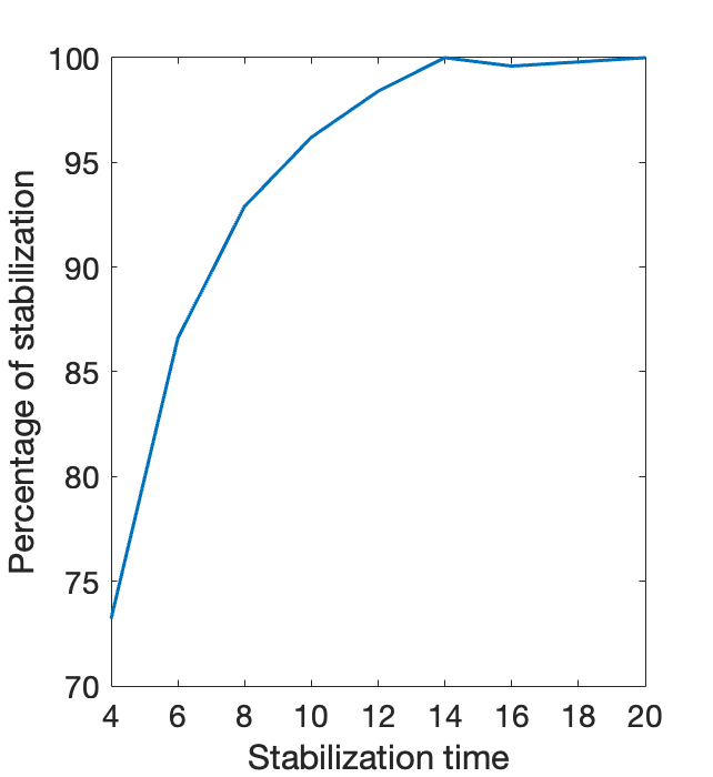
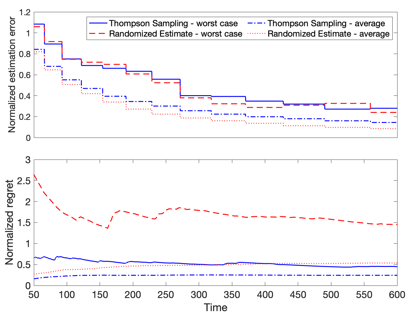
Figure 1: For the X-29A flight control problem, percentage of stabilization for 1000 runs of Algorithm 1 is plotted on the left. The graphs on the right depict the performance of Algorithm 2 (blue) compared to Randomized Estimate policy (red) [2]. The top graph plots the normalized squared estimation error, ${\left|\kern-1.29167pt\left|\boldsymbol{\widehat{\theta}_{n}}-\boldsymbol{\theta_{0}}\right|\kern-1.29167pt\right|}^{2}$ divided by $p(p+q)\boldsymbol{\tau}_{n}^{-1/2}\log\boldsymbol{\tau}_{n}$, versus time, while the lower one showcases the regret $\mathrm{Reg}\left(T\right)$, normalized by $p(p+q)T^{1/2}\log T$. Curves for the worst-case among $100$ replications are provided for both quantities, as well as for the averages over all replicates.

7 Concluding Remarks and Future Work

We studied Thompson sampling (TS) RL policies to control a diffusion process with unknown drift matrices. First, we proposed a stabilization algorithm for linear diffusion processes, and established that its failure probability decays exponentially with time. Further, efficiency of TS in balancing exploration versus exploitation for minimizing a quadratic cost function is shown. More precisely, regret bounds growing as square-root of time and square of dimensions are established for Algorithm 2. Empirical studies showcasing superiority of TS over state-of-the-art are provided as well.

As the first theoretical analysis of TS for control of a continuous-time model, this work implies multiple important future directions. Establishing minimax regret lower-bounds for diffusion process control problem is yet unanswered. Moreover, studying the performance of TS for robust control of the diffusion processes aiming to simultaneously minimize the cost function for a family of drift matrices, is also an interesting direction for further investigation. Another problem of interest is efficiency of TS for learning to control under partial observation where the state is not observed and instead a noisy linear function of the state is available as the output signal.

Organization of Appendices

This paper has four appendices. First, we prove Theorem 1 in Appendix A, together with multiple lemmas that the proof of the theorem relies on, and their statements and proofs are provided in Appendix A as well. Similarly, the proof for Theorem 2 together with intermediate steps, all are presented in Appendix B. Then, Appendix C consists of statements and proofs of other results that are used for establishing both theorems. Finally, empirical simulations beyond those presented in Section 6 are presented in Appendix D.

Appendix A Proof of Theorem 1

For analyzing the estimation error, we establish Lemma 4, which under the condition $\boldsymbol{\kappa_{\mathrm{}}}\gtrsim\boldsymbol{\tau}^{2}$ provides that with probability at least $1-\delta$,

$${\left|\kern-1.29167pt\left|\boldsymbol{\widehat{\theta}}-\boldsymbol{\theta_{0}}\right|\kern-1.29167pt\right|}\lesssim\frac{p\left(p+q\right)^{1/2}}{\boldsymbol{\tau}^{1/2}}\frac{\overline{\lambda}\left(\Sigma_{\mathbb{W}}\right)\vee\sigma_{w}^{2}}{\underline{\lambda}\left(\Sigma_{\mathbb{W}}\right)\wedge\sigma_{w}^{2}}\left(1+{\left|\kern-1.29167pt\left|K\right|\kern-1.29167pt\right|}\right)^{3}\log\left(\frac{pq\boldsymbol{\kappa_{\mathrm{}}}}{\delta}\right).$$

Note that in the proof of Lemma 4, results of Lemmas 1, 2, and 3 are used.

Therefore, Lemma 12 implies that for solutions of (5), with probability at least $1-\delta$, it holds that

$${\left|\kern-1.29167pt\left|{P}\left(\boldsymbol{\widehat{\theta}}\right)-{P}\left(\boldsymbol{\theta_{0}}\right)\right|\kern-1.29167pt\right|}\lesssim\frac{p\left(p+q\right)^{1/2}}{\boldsymbol{\tau}^{1/2}}\frac{\overline{\lambda}\left(\Sigma_{\mathbb{W}}\right)\vee\sigma_{w}^{2}}{\underline{\lambda}\left(\Sigma_{\mathbb{W}}\right)\wedge\sigma_{w}^{2}}\left(1+{\left|\kern-1.29167pt\left|K\right|\kern-1.29167pt\right|}\right)^{3}\log\left(\frac{pq\boldsymbol{\kappa_{\mathrm{}}}}{\delta}\right).$$

Note that we get the same expression as the right-hand-side above, as an upper bound for ${\left|\kern-1.29167pt\left|\widehat{B}^{\top}{P}\left(\boldsymbol{\widehat{\theta}}\right)-B_{0}^{\top}{P}\left(\boldsymbol{\theta_{0}}\right)\right|\kern-1.29167pt\right|}$. So, letting

$$\overline{A}=A_{0}-B_{0}Q_{u}^{-1}\widehat{B}^{\top}{P}\left(\boldsymbol{\widehat{\theta}}\right),~{}~{}~{}~{}~{}~{}~{}~{}\overline{A}_{0}=A_{0}-B_{0}Q_{u}^{-1}B_{0}^{\top}{P}\left(\boldsymbol{\theta_{0}}\right),$$

we obtain

$${\left|\kern-1.29167pt\left|\overline{A}-\overline{A}_{0}\right|\kern-1.29167pt\right|}\lesssim\sqrt{\frac{p^{2}q}{\boldsymbol{\tau}}}\frac{\overline{\lambda}\left(\Sigma_{\mathbb{W}}\right)\vee\sigma_{w}^{2}}{\underline{\lambda}\left(\Sigma_{\mathbb{W}}\right)\wedge\sigma_{w}^{2}}\left(1+{\left|\kern-1.29167pt\left|K\right|\kern-1.29167pt\right|}\right)^{3}\log\left(\frac{pq\boldsymbol{\kappa_{\mathrm{}}}}{\delta}\right),$$ (13)

with probability at least $1-\delta$.

Next, to consider the effect of the above errors on the eigenvalues of $\overline{A}$, we compare them to that of $\overline{A}_{0}$. Note that real-parts of all eigenvalues of $\overline{A}_{0}$ are at most $-\boldsymbol{\zeta_{0}}$, as defined in (10). So, using the result and the notation of Lemma 5, for all eigenvalues of $\overline{A}$ being on the open left half-plane it suffices to have $\Delta_{\overline{A}_{0}}\left(\overline{A}-\overline{A}_{0}\right)\leq\boldsymbol{\zeta_{0}}$. Also, in lights of Lemma 5, suppose that $\boldsymbol{r}$ is the size of the largest block in the Jordan block-diagonalization of $\overline{A}_{0}$. So, (36) implies that if

$${\left|\kern-1.29167pt\left|\overline{A}-\overline{A}_{0}\right|\kern-1.29167pt\right|}\lesssim\boldsymbol{r}^{-1/2}\left(1\wedge\boldsymbol{\zeta_{0}}^{\boldsymbol{r}}\right),$$

then Algorithm 1 successfully stabilizes the diffusion process in (1). Thus, (13) shows that the failure probability of Algorithm 1; $\mathbb{P}{\left(\mathcal{E}_{\boldsymbol{\tau}}\right)}$, satisfies

$$\sqrt{\frac{p^{2}q}{\boldsymbol{\tau}}}\frac{\overline{\lambda}\left(\Sigma_{\mathbb{W}}\right)\vee\sigma_{w}^{2}}{\underline{\lambda}\left(\Sigma_{\mathbb{W}}\right)\wedge\sigma_{w}^{2}}\left(1+{\left|\kern-1.29167pt\left|K\right|\kern-1.29167pt\right|}\right)^{3}\log\left(\frac{pq\boldsymbol{\kappa_{\mathrm{}}}}{\mathbb{P}{\left(\mathcal{E}_{\boldsymbol{\tau}}\right)}}\right)\gtrsim\boldsymbol{r}^{-1/2}\left(1\wedge\boldsymbol{\zeta_{0}}^{\boldsymbol{r}}\right).$$

Finally, $\boldsymbol{r}\leq p$ together with $\log\left(pq\boldsymbol{\kappa_{\mathrm{}}}\right)\lesssim\boldsymbol{\tau}^{1/2}$, lead to the desired result.

In the remainder of this section, technical lemmas above are stated and their proofs will be provided.

A.1 Bounding cross products of state and randomization

Definition 2

For a set $\mathcal{S}$, let $\mathds{1}{\left\{\mathcal{S}\right\}}$ be the indicator function that is $1$ on $\mathcal{S}$, and vanishes outside of $\mathcal{S}$.

Lemma 1

In Algorithm 1, for $t\geq 0$, define the piecewise-constant signal $v(t)$ below according to the randomization sequence $w_{n}$:

$$v(t)=\sum\limits_{n=0}^{\boldsymbol{\kappa_{\mathrm{}}}-1}\mathds{1}{\left\{\frac{n\boldsymbol{\tau}}{\boldsymbol{\kappa_{\mathrm{}}}}\leq t<\frac{(n+1)\boldsymbol{\tau}}{\boldsymbol{\kappa_{\mathrm{}}}}\right\}}w_{n}.$$ (14)

Then, with probability at least $1-\delta$, we have

$${{\left|\kern-1.29167pt\left|\int\limits_{0}^{\boldsymbol{\tau}}{\boldsymbol{x}_{s}v(s)^{\top}}\boldsymbol{d}{s}-\frac{\boldsymbol{\tau}^{2}}{2\boldsymbol{\kappa_{\mathrm{}}}^{2}}B_{0}\sum\limits_{n=0}^{\boldsymbol{\kappa_{\mathrm{}}}-1}w_{n}w_{n}^{\top}\right|\kern-1.29167pt\right|}}$$

$$\lesssim {\left(\sigma_{w}^{2}+\overline{\lambda}\left(\Sigma_{\mathbb{W}}\right)\right)\left(1+\int\limits_{0}^{\boldsymbol{\tau}}{{\left|\kern-1.29167pt\left|e^{\overline{A}t}\right|\kern-1.29167pt\right|}}\boldsymbol{d}{t}\right)}\left(pq^{1/2}\boldsymbol{\tau}^{1/2}\log\frac{pq}{\delta}+q\left[1+\frac{\boldsymbol{\tau}^{2}}{\boldsymbol{\kappa_{\mathrm{}}}^{2}}\right]\frac{\boldsymbol{\tau}}{\boldsymbol{\kappa_{\mathrm{}}}^{1/2}}\log^{3/2}\frac{\boldsymbol{\kappa_{\mathrm{}}}q}{\delta}\right).$$

Proof. First, after plugging the control signal $\boldsymbol{u}_{t}$ in (1) and solving the resulting stochastic differential equation, we obtain

$$\boldsymbol{x}_{t}=e^{\overline{A}t}\boldsymbol{x}_{0}+\int\limits_{0}^{t}{e^{\overline{A}(t-s)}}\boldsymbol{d}{\mathbb{W}_{s}}+\int\limits_{0}^{t}{e^{\overline{A}(t-s)}B_{0}v(s)}\boldsymbol{d}{s}.$$ (15)

This implies that

$$\int\limits_{0}^{\boldsymbol{\tau}}{\boldsymbol{x}_{t}v(t)^{\top}}\boldsymbol{d}{t}=\Phi_{1}+\Phi_{2}+\Phi_{3},$$

where

$$\Phi_{1} = \int\limits_{0}^{\boldsymbol{\tau}}{e^{\overline{A}t}\boldsymbol{x}_{0}v(t)^{\top}}\boldsymbol{d}{t}=\sum\limits_{n=0}^{\boldsymbol{\kappa_{\mathrm{}}}-1}\left(\int\limits_{n\boldsymbol{\tau}\boldsymbol{\kappa_{\mathrm{}}}^{-1}}^{(n+1)\boldsymbol{\tau}\boldsymbol{\kappa_{\mathrm{}}}^{-1}}{e^{\overline{A}t}}\boldsymbol{d}{t}\right)\boldsymbol{x}_{0}w_{n}^{\top},$$

$$\Phi_{2} = \int\limits_{0}^{\boldsymbol{\tau}}{\int\limits_{0}^{t}{e^{\overline{A}(t-s)}}\boldsymbol{d}{\mathbb{W}_{s}}v(t)^{\top}}\boldsymbol{d}{t}=\sum\limits_{n=0}^{\boldsymbol{\kappa_{\mathrm{}}}-1}\left(\int\limits_{n\boldsymbol{\tau}\boldsymbol{\kappa_{\mathrm{}}}^{-1}}^{(n+1)\boldsymbol{\tau}\boldsymbol{\kappa_{\mathrm{}}}^{-1}}{\int\limits_{0}^{t}{e^{\overline{A}(t-s)}}\boldsymbol{d}{\mathbb{W}_{s}}}\boldsymbol{d}{t}\right)w_{n}^{\top},$$

$$\Phi_{3} = \int\limits_{0}^{\boldsymbol{\tau}}{\int\limits_{0}^{t}{e^{\overline{A}(t-s)}B_{0}v(s)}\boldsymbol{d}{s}v(t)^{\top}}\boldsymbol{d}{t}.$$

To analyze $\Phi_{1}$, we use the fact that every entry of $\Phi_{1}$ is a normal random variable with mean zero and variance at most

$$\sigma_{w}^{2}\sum\limits_{n=0}^{\boldsymbol{\kappa_{\mathrm{}}}-1}{\left|\kern-1.29167pt\left|\int\limits_{n\boldsymbol{\tau}\boldsymbol{\kappa_{\mathrm{}}}^{-1}}^{(n+1)\boldsymbol{\tau}\boldsymbol{\kappa_{\mathrm{}}}^{-1}}{e^{\overline{A}t}}\boldsymbol{d}{t}\right|\kern-1.29167pt\right|}^{2}{\left|\kern-1.50696pt\left|\boldsymbol{x}_{0}\right|\kern-1.50696pt\right|}^{2}\leq\sigma_{w}^{2}\left(\int\limits_{0}^{\boldsymbol{\tau}}{{\left|\kern-1.29167pt\left|e^{\overline{A}t}\right|\kern-1.29167pt\right|}}\boldsymbol{d}{t}\right)^{2}{\left|\kern-1.50696pt\left|\boldsymbol{x}_{0}\right|\kern-1.50696pt\right|}^{2}.$$

Therefore, with probability at least $1-\delta$, it holds that

$${\left|\kern-1.29167pt\left|\Phi_{1}\right|\kern-1.29167pt\right|}\lesssim\sigma_{w}\left(\int\limits_{0}^{\boldsymbol{\tau}}{{\left|\kern-1.29167pt\left|e^{\overline{A}t}\right|\kern-1.29167pt\right|}}\boldsymbol{d}{t}\right){\left|\kern-1.50696pt\left|\boldsymbol{x}_{0}\right|\kern-1.50696pt\right|}\sqrt{pq\log\left(\frac{pq}{\delta}\right)}.$$ (16)

Furthermore, to study $\Phi_{2}$, Fubini Theorem [37] gives

$$\int\limits_{n\boldsymbol{\tau}\boldsymbol{\kappa_{\mathrm{}}}^{-1}}^{(n+1)\boldsymbol{\tau}\boldsymbol{\kappa_{\mathrm{}}}^{-1}}{\int\limits_{0}^{t}{e^{\overline{A}(t-s)}}\boldsymbol{d}{\mathbb{W}_{s}}}\boldsymbol{d}{t} = \int\limits_{0}^{n\boldsymbol{\tau}\boldsymbol{\kappa_{\mathrm{}}}^{-1}}{\left(\int\limits_{n\boldsymbol{\tau}\boldsymbol{\kappa_{\mathrm{}}}^{-1}}^{(n+1)\boldsymbol{\tau}\boldsymbol{\kappa_{\mathrm{}}}^{-1}}{e^{\overline{A}(t-n\boldsymbol{\tau}\boldsymbol{\kappa_{\mathrm{}}}^{-1})}}\boldsymbol{d}{t}\right)e^{\overline{A}(n\boldsymbol{\tau}\boldsymbol{\kappa_{\mathrm{}}}^{-1}-s)}}\boldsymbol{d}{\mathbb{W}_{s}}$$

$$+ \int\limits_{n\boldsymbol{\tau}\boldsymbol{\kappa_{\mathrm{}}}^{-1}}^{(n+1)\boldsymbol{\tau}\boldsymbol{\kappa_{\mathrm{}}}^{-1}}{\left(\int\limits_{s}^{(n+1)\boldsymbol{\tau}\boldsymbol{\kappa_{\mathrm{}}}^{-1}}{e^{\overline{A}(t-s)}}\boldsymbol{d}{t}\right)}\boldsymbol{d}{\mathbb{W}_{s}}$$

$$= F\sum\limits_{m=1}^{n}e^{\overline{A}(n-m)\boldsymbol{\tau}\boldsymbol{\kappa_{\mathrm{}}}^{-1}}\int\limits_{(m-1)\boldsymbol{\tau}\boldsymbol{\kappa_{\mathrm{}}}^{-1}}^{m\boldsymbol{\tau}\boldsymbol{\kappa_{\mathrm{}}}^{-1}}{e^{\overline{A}(m\boldsymbol{\tau}\boldsymbol{\kappa_{\mathrm{}}}^{-1}-s)}}\boldsymbol{d}{\mathbb{W}_{s}}$$

$$+ \int\limits_{n\boldsymbol{\tau}\boldsymbol{\kappa_{\mathrm{}}}^{-1}}^{(n+1)\boldsymbol{\tau}\boldsymbol{\kappa_{\mathrm{}}}^{-1}}{G_{s}}\boldsymbol{d}{\mathbb{W}_{s}}$$

where the matrix $F=\int\limits_{n\boldsymbol{\tau}\boldsymbol{\kappa_{\mathrm{}}}^{-1}}^{(n+1)\boldsymbol{\tau}\boldsymbol{\kappa_{\mathrm{}}}^{-1}}{e^{\overline{A}(t-n\boldsymbol{\tau}\boldsymbol{\kappa_{\mathrm{}}}^{-1})}}\boldsymbol{d}{t}$, does not depend on $s$ or $n$, and the matrix $G_{s}=\int\limits_{s}^{(n+1)\boldsymbol{\tau}\boldsymbol{\kappa_{\mathrm{}}}^{-1}}{e^{\overline{A}(t-s)}}\boldsymbol{d}{t}$, does not depend on $n$, since $n\boldsymbol{\tau}\boldsymbol{\kappa_{\mathrm{}}}^{-1}\leq s\leq(n+1)\boldsymbol{\tau}\boldsymbol{\kappa_{\mathrm{}}}^{-1}$.

So, letting $\mathrm{e}_{i},i=1,\cdots,p$, be the standard basis of the Euclidean space, conditioned on the Wiener process $\left\{\mathbb{W}_{s}\right\}_{s\geq 0}$, for every $j=1,\cdots,q$, the coordinate $j$ of $\mathrm{e}_{i}^{\top}\Phi_{2}$ is a mean zero normal random variable. Thus, given $\left\{\mathbb{W}_{s}\right\}_{s\geq 0}$, with probability at least $1-\delta$, it holds that

$$\left(\mathrm{e}_{i}^{\top}\Phi_{2}\mathrm{e}_{j}\right)^{2}\lesssim\mathrm{var\left(\mathrm{e}_{i}^{\top}\Phi_{2}\mathrm{e}_{j}\Big{|}\mathcal{F}\left(\mathbb{W}_{0:\boldsymbol{\tau}}\right)\right)}\log\frac{1}{\delta}.$$

Now, to calculate the conditional variance, we can write

$$\frac{\mathrm{var\left(\mathrm{e}_{i}^{\top}\Phi_{2}\mathrm{e}_{j}\Big{|}\mathcal{F}\left(\mathbb{W}_{0:\boldsymbol{\tau}}\right)\right)}}{\sigma_{w}^{2}}=\sum\limits_{n=0}^{\boldsymbol{\kappa_{\mathrm{}}}-1}\left[\mathrm{e}_{i}^{\top}\int\limits_{n\boldsymbol{\tau}\boldsymbol{\kappa_{\mathrm{}}}^{-1}}^{(n+1)\boldsymbol{\tau}\boldsymbol{\kappa_{\mathrm{}}}^{-1}}{\int\limits_{0}^{t}{e^{\overline{A}(t-s)}}\boldsymbol{d}{\mathbb{W}_{s}}}\boldsymbol{d}{t}\right]^{2}\lesssim\sum\limits_{n=1}^{\boldsymbol{\kappa_{\mathrm{}}}-1}\left[\left(\sum\limits_{m=1}^{n}\beta_{m,n}\right)^{2}+\alpha_{n}^{2}\right],$$

where

$$\beta_{m,n} = \mathrm{e}_{i}^{\top}Fe^{\overline{A}(n-m)\boldsymbol{\tau}\boldsymbol{\kappa_{\mathrm{}}}^{-1}}\int\limits_{(m-1)\boldsymbol{\tau}\boldsymbol{\kappa_{\mathrm{}}}^{-1}}^{m\boldsymbol{\tau}\boldsymbol{\kappa_{\mathrm{}}}^{-1}}{e^{\overline{A}(m\boldsymbol{\tau}\boldsymbol{\kappa_{\mathrm{}}}^{-1}-s)}}\boldsymbol{d}{\mathbb{W}_{s}},$$

$$\alpha_{n} = \mathrm{e}_{i}^{\top}\int\limits_{n\boldsymbol{\tau}\boldsymbol{\kappa_{\mathrm{}}}^{-1}}^{(n+1)\boldsymbol{\tau}\boldsymbol{\kappa_{\mathrm{}}}^{-1}}{G_{s}}\boldsymbol{d}{\mathbb{W}_{s}}.$$

To proceed, define the matrix $H=\left[H_{n,m}\right]$, where for $1\leq m,n\leq\boldsymbol{\kappa_{\mathrm{}}}-1$, every block $H_{n,m}\in\mathbb{R}^{1\times p}$ is

$$H_{n,m}=\mathrm{e}_{i}^{\top}Fe^{\overline{A}(n-m)\boldsymbol{\tau}\boldsymbol{\kappa_{\mathrm{}}}^{-1}},$$

for $m\leq n$, and is $0$ for $m>n$. Then, denote

$$\Gamma=\begin{bmatrix}\int\limits_{0}^{\boldsymbol{\tau}\boldsymbol{\kappa_{\mathrm{}}}^{-1}}{e^{\overline{A}(\boldsymbol{\tau}\boldsymbol{\kappa_{\mathrm{}}}^{-1}-s)}}\boldsymbol{d}{\mathbb{W}_{s}}\\ \int\limits_{\boldsymbol{\tau}\boldsymbol{\kappa_{\mathrm{}}}^{-1}}^{2\boldsymbol{\tau}\boldsymbol{\kappa_{\mathrm{}}}^{-1}}{e^{\overline{A}(2\boldsymbol{\tau}\boldsymbol{\kappa_{\mathrm{}}}^{-1}-s)}}\boldsymbol{d}{\mathbb{W}_{s}}\\ \vdots\\ \int\limits_{(\boldsymbol{\kappa_{\mathrm{}}}-1)\boldsymbol{\tau}\boldsymbol{\kappa_{\mathrm{}}}^{-1}}^{\boldsymbol{\tau}}{e^{\overline{A}(\boldsymbol{\tau}-s)}}\boldsymbol{d}{\mathbb{W}_{s}}\end{bmatrix}\in\mathbb{R}^{p(\boldsymbol{\kappa_{\mathrm{}}}-1)\times 1},$$

to get

$$\sum\limits_{n=0}^{\boldsymbol{\kappa_{\mathrm{}}}-1}\left(\sum\limits_{m=1}^{n}\beta_{m,n}^{2}\right)={\left|\kern-1.50696pt\left|H\Gamma\right|\kern-1.50696pt\right|}^{2}\leq\overline{\lambda}\left(H^{\top}H\right){\left|\kern-1.50696pt\left|\Gamma\right|\kern-1.50696pt\right|}^{2}.$$

Now, for the matrix $H$, we have [48, 49]:

$$\overline{\lambda}\left(H^{\top}H\right)\lesssim\left(\sum\limits_{n=1}^{\boldsymbol{\kappa_{\mathrm{}}}-1}{\left|\kern-1.50696pt\left|H_{n,1}\right|\kern-1.50696pt\right|}\right)^{2}\lesssim\left(\boldsymbol{\tau}\boldsymbol{\kappa_{\mathrm{}}}^{-1}\sum\limits_{n=1}^{\boldsymbol{\kappa_{\mathrm{}}}}e^{\overline{A}n\boldsymbol{\tau}\boldsymbol{\kappa_{\mathrm{}}}^{-1}}\right)^{2}\lesssim\left(\int\limits_{0}^{\boldsymbol{\tau}}{{\left|\kern-1.29167pt\left|e^{\overline{A}t}\right|\kern-1.29167pt\right|}}\boldsymbol{d}{t}\right)^{2}.$$

Note that thanks to the independent increments of the Wiener process, the blocks of $\Gamma$ are statistically independent. Further, by Ito Isometry [37], every block of $\Gamma$ is a mean-zero normally distributed vector with the covariance matrix

$$\int\limits_{0}^{\boldsymbol{\tau}\boldsymbol{\kappa_{\mathrm{}}}^{-1}}{e^{\overline{A}(\boldsymbol{\tau}\boldsymbol{\kappa_{\mathrm{}}}^{-1}-s)}\Sigma_{\mathbb{W}}e^{\overline{A}^{\top}(\boldsymbol{\tau}\boldsymbol{\kappa_{\mathrm{}}}^{-1}-s)}}\boldsymbol{d}{s}.$$

So, according to the exponential inequalities for quadratic forms of normally distributed random variables [45], it holds with probability at least $1-\delta$, that

$${\left|\kern-1.50696pt\left|\Gamma\right|\kern-1.50696pt\right|}^{2}\lesssim p\boldsymbol{\kappa_{\mathrm{}}}\overline{\lambda}\left(\Sigma_{\mathbb{W}}\right)\left(\boldsymbol{\tau}\boldsymbol{\kappa_{\mathrm{}}}^{-1}\right)\log\frac{1}{\delta}.$$

Thus, with probability at least $1-\delta$, we have

$$\sum\limits_{n=0}^{\boldsymbol{\kappa_{\mathrm{}}}-1}\left(\sum\limits_{m=1}^{n}\beta_{m,n}^{2}\right)\lesssim\left(\int\limits_{0}^{\boldsymbol{\tau}}{{\left|\kern-1.29167pt\left|e^{\overline{A}t}\right|\kern-1.29167pt\right|}}\boldsymbol{d}{t}\right)^{2}p\overline{\lambda}\left(\Sigma_{\mathbb{W}}\right)\boldsymbol{\tau}\log\frac{1}{\delta}.$$

Similarly, the bound above can be shown for $\sum\limits_{n=1}^{\boldsymbol{\kappa_{\mathrm{}}}-1}\alpha_{n}^{2}$. Hence, we obtain the corresponding high probability bound for a single entry $\mathrm{e}_{i}^{\top}\Phi_{2}\mathrm{e}_{j}$ of $\Phi_{2}$, which together with a union bound, implies that

$${\left|\kern-1.29167pt\left|\Phi_{2}\right|\kern-1.29167pt\right|}\lesssim\sigma_{w}pq^{1/2}\left(\int\limits_{0}^{\boldsymbol{\tau}}{{\left|\kern-1.29167pt\left|e^{\overline{A}t}\right|\kern-1.29167pt\right|}}\boldsymbol{d}{t}\right)\overline{\lambda}\left(\Sigma_{\mathbb{W}}\right)^{1/2}\boldsymbol{\tau}^{1/2}\log\left(\frac{pq}{\delta}\right),$$ (17)

with probability at least $1-\delta$.

Next, according to Fubini Theorem, $\Phi_{3}$ can also be written as

$$\Phi_{3} = \int\limits_{0}^{\boldsymbol{\tau}}{\int\limits_{0}^{s}{e^{\overline{A}(s-t)}B_{0}v(t)v(s)^{\top}}\boldsymbol{d}{t}}\boldsymbol{d}{s}=\int\limits_{0}^{\boldsymbol{\tau}}{\int\limits_{t}^{\boldsymbol{\tau}}{e^{\overline{A}(s-t)}B_{0}v(t)v(s)^{\top}}\boldsymbol{d}{s}}\boldsymbol{d}{t}.$$

Thus, we have

$$2\Phi_{3}=\int\limits_{0}^{\boldsymbol{\tau}}{\int\limits_{0}^{\boldsymbol{\tau}}{e^{\overline{A}\left|t-s\right|}B_{0}v(t\wedge s)v(s\vee t)^{\top}}\boldsymbol{d}{t}}\boldsymbol{d}{s}.$$

Recall that the signal $v(t)$ in (14) is piecewise-constant, with values determined by the randomization sequence $w_{n}$. So, the above double integral can be written as a double sum

$$2\Phi_{3} = \sum\limits_{n=0}^{\boldsymbol{\kappa_{\mathrm{}}}-1}\sum\limits_{m=0}^{\boldsymbol{\kappa_{\mathrm{}}}-1}\left(\int\limits_{n\boldsymbol{\tau}\boldsymbol{\kappa_{\mathrm{}}}^{-1}}^{(n+1)\boldsymbol{\tau}\boldsymbol{\kappa_{\mathrm{}}}^{-1}}{\int\limits_{m\boldsymbol{\tau}\boldsymbol{\kappa_{\mathrm{}}}^{-1}}^{(m+1)\boldsymbol{\tau}\boldsymbol{\kappa_{\mathrm{}}}^{-1}}{e^{\overline{A}\left|t-s\right|}}\boldsymbol{d}{s}}\boldsymbol{d}{t}\right)B_{0}w_{m\wedge n}w_{m\vee n}^{\top}$$

$$= \sum\limits_{n=0}^{\boldsymbol{\kappa_{\mathrm{}}}-1}\sum\limits_{m=0}^{\boldsymbol{\kappa_{\mathrm{}}}-1}\left(e^{\overline{A}\left|m-n\right|\boldsymbol{\tau}\boldsymbol{\kappa_{\mathrm{}}}^{-1}}\int\limits_{0}^{\boldsymbol{\tau}\boldsymbol{\kappa_{\mathrm{}}}^{-1}}{\int\limits_{0}^{\boldsymbol{\tau}\boldsymbol{\kappa_{\mathrm{}}}^{-1}}{e^{\overline{A}\left|t-s\right|}}\boldsymbol{d}{s}}\boldsymbol{d}{t}\right)B_{0}w_{m\wedge n}w_{m\vee n}^{\top}.$$

Thus, we have

$$2\Phi_{3}-\frac{\boldsymbol{\tau}^{2}}{\boldsymbol{\kappa_{\mathrm{}}}^{2}}B_{0}\sum\limits_{n=0}^{\boldsymbol{\kappa_{\mathrm{}}}-1}w_{n}w_{n}^{\top}=\Phi_{4}+\Phi_{5},$$ (18)

for

$$\Phi_{4} = \left(\int\limits_{0}^{\boldsymbol{\tau}\boldsymbol{\kappa_{\mathrm{}}}^{-1}}{\int\limits_{0}^{\boldsymbol{\tau}\boldsymbol{\kappa_{\mathrm{}}}^{-1}}{e^{\overline{A}\left|t-s\right|}}\boldsymbol{d}{s}}\boldsymbol{d}{t}-\boldsymbol{\tau}^{2}\boldsymbol{\kappa_{\mathrm{}}}^{-2}I_{q}\right)B_{0}\sum\limits_{n=0}^{\boldsymbol{\kappa_{\mathrm{}}}-1}w_{n}w_{n}^{\top},$$

$$\Phi_{5} = 2\left(\int\limits_{0}^{\boldsymbol{\tau}\boldsymbol{\kappa_{\mathrm{}}}^{-1}}{\int\limits_{0}^{\boldsymbol{\tau}\boldsymbol{\kappa_{\mathrm{}}}^{-1}}{e^{\overline{A}\left|t-s\right|}}\boldsymbol{d}{s}}\boldsymbol{d}{t}\right)\sum\limits_{n=0}^{\boldsymbol{\kappa_{\mathrm{}}}-1}\sum\limits_{m=n+1}^{\boldsymbol{\kappa_{\mathrm{}}}-1}\left(e^{\overline{A}\left(m-n\right)\boldsymbol{\tau}\boldsymbol{\kappa_{\mathrm{}}}^{-1}}B_{0}w_{n}w_{m}^{\top}\right).$$

To proceed, we use the following concentration inequality for random matrices with martingale difference structures, titled as Matrix Azuma inequality [46].

Theorem 3

Let $\left\{\Psi_{n}\right\}_{n=1}^{k}$ be a $d_{1}\times d_{2}$ martingale difference sequence. That is, for some filtration $\left\{\mathcal{F}_{n}\right\}_{n=0}^{k}$, the matrix $\Psi_{n}$ is $\mathcal{F}_{n}$-measurable, and $\mathbb{E}\left[\Psi_{n}\Big{|}\mathcal{F}_{n-1}\right]=0$. Suppose that ${\left|\kern-1.29167pt\left|\Psi_{n}\right|\kern-1.29167pt\right|}\leq\sigma_{n}$, for some fixed sequence $\left\{\sigma_{n}\right\}_{n=1}^{k}$. Then, with probability at least $1-\delta$, we have

$${\left|\kern-1.29167pt\left|\sum\limits_{n=1}^{k}\Psi_{n}\right|\kern-1.29167pt\right|}^{2}\lesssim\left(\sum\limits_{n=1}^{k}\sigma_{n}^{2}\right)\log\frac{d_{1}+d_{2}}{\delta}.$$

So, to study $\Phi_{4}$, we apply Theorem 3 to the random matrices $\Psi_{n}=w_{n}w_{n}^{\top}-\sigma_{w}^{2}I_{q}$, using the trivial filtration and the high probability upper-bounds for ${\left|\kern-1.29167pt\left|\Psi_{n}\right|\kern-1.29167pt\right|}\leq{\left|\kern-1.50696pt\left|w_{n}\right|\kern-1.50696pt\right|}^{2}+\sigma_{w}^{2}$;

$${\left|\kern-1.29167pt\left|\Psi_{n}\right|\kern-1.29167pt\right|}\leq\sigma_{n}=\sigma_{w}^{2}\left(1+q\log\frac{q\boldsymbol{\kappa_{\mathrm{}}}}{\delta}\right),$$

as well as the fact

$${\left|\kern-1.29167pt\left|\int\limits_{0}^{\boldsymbol{\tau}\boldsymbol{\kappa_{\mathrm{}}}^{-1}}{\int\limits_{0}^{\boldsymbol{\tau}\boldsymbol{\kappa_{\mathrm{}}}^{-1}}{\left(e^{\overline{A}\left|t-s\right|}-I_{q}\right)}\boldsymbol{d}{s}}\boldsymbol{d}{t}\right|\kern-1.29167pt\right|}\lesssim\boldsymbol{\tau}^{3}\boldsymbol{\kappa_{\mathrm{}}}^{-3},$$

to obtain the following bound, which holds with probability at least $1-\delta$:

$${\left|\kern-1.29167pt\left|\Phi_{4}\right|\kern-1.29167pt\right|}\lesssim{\left|\kern-1.29167pt\left|B_{0}\right|\kern-1.29167pt\right|}\sigma_{w}^{2}\boldsymbol{\tau}^{3}\boldsymbol{\kappa_{\mathrm{}}}^{-2}\left(1+\frac{q}{\boldsymbol{\kappa_{\mathrm{}}}^{1/2}}\log^{3/2}\frac{\boldsymbol{\kappa_{\mathrm{}}}q}{\delta}\right).$$ (19)

On the other hand, to establish an upper-bound for $\Phi_{5}$, consider the random matrices

$$\Psi_{n}=\sum\limits_{m=n+1}^{\boldsymbol{\kappa_{\mathrm{}}}-1}\left(e^{\overline{A}\left(m-n\right)\boldsymbol{\tau}\boldsymbol{\kappa_{\mathrm{}}}^{-1}}B_{0}w_{n}w_{m}^{\top}\right),$$

subject to the natural filtration they generate, and apply Theorem 3, using the bounds

$${\left|\kern-1.29167pt\left|\Psi_{n}\right|\kern-1.29167pt\right|}\leq\sigma_{n}\lesssim\boldsymbol{\tau}^{-1}\boldsymbol{\kappa_{\mathrm{}}}\left(\int\limits_{0}^{\boldsymbol{\tau}}{{\left|\kern-1.29167pt\left|e^{\overline{A}t}\right|\kern-1.29167pt\right|}}\boldsymbol{d}{t}\right){\left|\kern-1.29167pt\left|B_{0}\right|\kern-1.29167pt\right|}\sigma_{w}^{2}q\log\frac{\boldsymbol{\kappa_{\mathrm{}}}q}{\delta},$$

together with

$${\left|\kern-1.29167pt\left|\int\limits_{0}^{\boldsymbol{\tau}\boldsymbol{\kappa_{\mathrm{}}}^{-1}}{\int\limits_{0}^{\boldsymbol{\tau}\boldsymbol{\kappa_{\mathrm{}}}^{-1}}{e^{\overline{A}\left|t-s\right|}}\boldsymbol{d}{s}}\boldsymbol{d}{t}\right|\kern-1.29167pt\right|}\lesssim\boldsymbol{\tau}^{2}\boldsymbol{\kappa_{\mathrm{}}}^{-2}.$$

Therefore, Theorem 3 indicates that with probability at least $1-\delta$, it holds that

$$\Phi_{5}\lesssim\frac{\boldsymbol{\tau}}{\boldsymbol{\kappa_{\mathrm{}}}^{1/2}}\left(\int\limits_{0}^{\boldsymbol{\tau}}{{\left|\kern-1.29167pt\left|e^{\overline{A}t}\right|\kern-1.29167pt\right|}}\boldsymbol{d}{t}\right){\left|\kern-1.29167pt\left|B_{0}\right|\kern-1.29167pt\right|}\sigma_{w}^{2}q\log^{3/2}\frac{\boldsymbol{\kappa_{\mathrm{}}}q}{\delta}.$$ (20)

Finally, put (16), (17), (18), (19), and (20) together, to get the desired result.

$\blacksquare$

A.2 Bounding cross products of state and Wiener process

Lemma 2

In Algorithm 1, with probability at least $1-\delta$, we have

$${\left|\kern-1.29167pt\left|\int\limits_{0}^{t}{\boldsymbol{x}_{s}}\boldsymbol{d}{\mathbb{W}_{s}^{\top}}\right|\kern-1.29167pt\right|}\lesssim\left(\int\limits_{0}^{\boldsymbol{\tau}}{{\left|\kern-1.29167pt\left|e^{\overline{A}t}\right|\kern-1.29167pt\right|}}\boldsymbol{d}{t}\right)\left(\overline{\lambda}\left(\Sigma_{\mathbb{W}}\right)+\sigma_{w}^{2}\right)p\left(p+q\right)^{1/2}\boldsymbol{\tau}^{1/2}\log\left(\frac{pq}{\delta}\right).$$

Proof. First, according to (15), we can write

$$\int\limits_{0}^{\boldsymbol{\tau}}{\boldsymbol{x}_{t}}\boldsymbol{d}{\mathbb{W}_{t}^{\top}}=\Phi_{1}+\Phi_{2}+\Phi_{3},$$

where

$$\Phi_{1} = \int\limits_{0}^{\boldsymbol{\tau}}{e^{\overline{A}t}\boldsymbol{x}_{0}}\boldsymbol{d}{\mathbb{W}_{t}^{\top}},$$ (21)

$$\Phi_{2} = \int\limits_{0}^{\boldsymbol{\tau}}{\int\limits_{0}^{t}{e^{\overline{A}(t-s)}B_{0}v(s)}\boldsymbol{d}{s}}\boldsymbol{d}{\mathbb{W}_{t}^{\top}},$$ (22)

$$\Phi_{3} = \int\limits_{0}^{\boldsymbol{\tau}}{\int\limits_{0}^{t}{e^{\overline{A}(t-s)}}\boldsymbol{d}{\mathbb{W}_{s}}}\boldsymbol{d}{\mathbb{W}_{t}^{\top}}.$$ (23)

Now, according to Ito Isometry [37], similar to (16), we have

$${\left|\kern-1.29167pt\left|\Phi_{1}\right|\kern-1.29167pt\right|}\lesssim\overline{\lambda}\left(\Sigma_{\mathbb{W}}\right)^{1/2}\left(\int\limits_{0}^{\boldsymbol{\tau}}{{\left|\kern-1.29167pt\left|e^{\overline{A}t}\right|\kern-1.29167pt\right|}}\boldsymbol{d}{t}\right){\left|\kern-1.50696pt\left|\boldsymbol{x}_{0}\right|\kern-1.50696pt\right|}\sqrt{pq\log\left(\frac{pq}{\delta}\right)},$$ (24)

with probability at least $1-\delta$. Moreover, in a procedure similar to the one that lead to (17), one can show that with probability at least $1-\delta$, it holds that

$${\left|\kern-1.29167pt\left|\Phi_{2}\right|\kern-1.29167pt\right|}\lesssim\left(\int\limits_{0}^{\boldsymbol{\tau}}{{\left|\kern-1.29167pt\left|e^{\overline{A}t}\right|\kern-1.29167pt\right|}}\boldsymbol{d}{t}\right)\overline{\lambda}\left(\Sigma_{\mathbb{W}}\right)^{1/2}\sigma_{w}pq^{1/2}\boldsymbol{\tau}^{1/2}\log\left(\frac{pq}{\delta}\right).$$ (25)

Therefore, we need to find a similar upper-bound for $\Phi_{3}$. To that end, Ito formula provides

$$\boldsymbol{d}\left(e^{-\overline{A}s}\mathbb{W}_{s}\right)=-\overline{A}e^{-\overline{A}s}\mathbb{W}_{s}\boldsymbol{d}s+e^{-\overline{A}s}\boldsymbol{d}\mathbb{W}_{s}.$$

Therefore, integration gives

$$\int\limits_{0}^{t}{e^{-\overline{A}s}}\boldsymbol{d}{\mathbb{W}_{s}}=e^{-\overline{A}t}\mathbb{W}_{t}+\overline{A}\int\limits_{0}^{t}{e^{-\overline{A}s}\mathbb{W}_{s}}\boldsymbol{d}{s},$$

which after rearranging and letting $\Psi_{t}=\int\limits_{0}^{t}{e^{\overline{A}(t-s)}}\boldsymbol{d}{\mathbb{W}_{s}}$, leads to

$$\Psi_{t}\mathbb{W}_{t}^{\top}=\left(\int\limits_{0}^{t}{e^{\overline{A}(t-s)}}\boldsymbol{d}{\mathbb{W}_{s}}\right){\mathbb{W}_{t}^{\top}}={\mathbb{W}_{t}}{\mathbb{W}_{t}^{\top}}+\overline{A}{\left(\int\limits_{0}^{t}{e^{\overline{A}(t-s)}\mathbb{W}_{s}}\boldsymbol{d}{s}\right)}{\mathbb{W}_{t}^{\top}}.$$

Now, since $\boldsymbol{d}\Psi_{t}=\boldsymbol{d}\mathbb{W}_{t}$, Ito Isometry [37] implies that $\boldsymbol{d}\Psi_{t}\boldsymbol{d}\mathbb{W}_{t}^{\top}=\Sigma_{\mathbb{W}}\boldsymbol{d}t$. So, apply integration by part and use the above equation to get

$$\Phi_{3}=\int\limits_{0}^{\boldsymbol{\tau}}{\Psi_{t}}\boldsymbol{d}{\mathbb{W}_{t}^{\top}} = \int\limits_{0}^{\boldsymbol{\tau}}{}\boldsymbol{d}{\left(\Psi_{t}\mathbb{W}_{t}^{\top}\right)}-\left(\int\limits_{0}^{\boldsymbol{\tau}}{\mathbb{W}_{t}}\boldsymbol{d}{\Psi_{t}^{\top}}\right)^{\top}-\int\limits_{0}^{\boldsymbol{\tau}}{\boldsymbol{d}\Psi_{t}}\boldsymbol{d}{\mathbb{W}_{t}^{\top}}$$

$$= {\Psi_{\boldsymbol{\tau}}}{\mathbb{W}_{\boldsymbol{\tau}}^{\top}}-\left(\int\limits_{0}^{\boldsymbol{\tau}}{\mathbb{W}_{t}}\boldsymbol{d}{\mathbb{W}_{t}^{\top}}\right)^{\top}-\Sigma_{\mathbb{W}}\boldsymbol{\tau}$$

$$= {\mathbb{W}_{\boldsymbol{\tau}}}{\mathbb{W}_{\boldsymbol{\tau}}^{\top}}+\overline{A}{\left(\int\limits_{0}^{\boldsymbol{\tau}}{e^{\overline{A}(\boldsymbol{\tau}-s)}\mathbb{W}_{s}}\boldsymbol{d}{s}\right)}{\mathbb{W}_{\boldsymbol{\tau}}^{\top}}-\left(\int\limits_{0}^{\boldsymbol{\tau}}{\mathbb{W}_{t}}\boldsymbol{d}{\mathbb{W}_{t}^{\top}}\right)^{\top}-\Sigma_{\mathbb{W}}\boldsymbol{\tau}.$$

Therefore, every entry of $\Phi_{3}$ is a quadratic function of the normally distributed random vectors $\mathbb{W}_{\boldsymbol{\tau}},\int\limits_{0}^{\boldsymbol{\tau}}{e^{\overline{A}(\boldsymbol{\tau}-s)}\mathbb{W}_{s}}\boldsymbol{d}{s}$. Note that we used the fact that

$$\mathbb{W}_{\boldsymbol{\tau}}\mathbb{W}_{\boldsymbol{\tau}}^{\top}=\int\limits_{0}^{\boldsymbol{\tau}}{}\boldsymbol{d}{\left(\mathbb{W}_{t}\mathbb{W}_{t}^{\top}\right)}=\left(\int\limits_{0}^{\boldsymbol{\tau}}{\mathbb{W}_{t}}\boldsymbol{d}{\mathbb{W}_{t}^{\top}}\right)^{\top}+\left(\int\limits_{0}^{\boldsymbol{\tau}}{\mathbb{W}_{t}}\boldsymbol{d}{\mathbb{W}_{t}^{\top}}\right)+\Sigma_{\mathbb{W}}\boldsymbol{\tau}.$$

Thus, exponential inequalities for quadratic forms of normal random vectors [45] imply that for all $i,j=1,\cdots,p$, it holds that

$$\left(\mathrm{e}_{i}^{\top}\Phi_{3}\mathrm{e}_{j}\right)^{2}\lesssim p\mathbb{E}\left[\left(\mathrm{e}_{i}^{\top}\Phi_{3}\mathrm{e}_{j}\right)^{2}\right]\log^{2}\frac{1}{\delta},$$ (26)

since $\mathbb{E}\left[\mathrm{e}_{i}^{\top}\Phi_{3}\mathrm{e}_{j}\right]=0$. So, it suffices to find the expectation in (26). For that purpose, we use Ito Isometry [37] to obtain:

$$\mathbb{E}\left[\left(\mathrm{e}_{i}^{\top}\Phi_{3}\mathrm{e}_{j}\right)^{2}\right] = \mathbb{E}\left[\left(\int\limits_{0}^{\boldsymbol{\tau}}{\mathrm{e}_{i}^{\top}\Psi_{t}\mathrm{e}_{j}^{\top}\Sigma_{\mathbb{W}}^{1/2}}\boldsymbol{d}{\left(\Sigma_{\mathbb{W}}^{-1/2}\mathbb{W}_{t}\right)}\right)^{2}\right]=\mathbb{E}\left[\int\limits_{0}^{\boldsymbol{\tau}}{{\left|\kern-1.50696pt\left|\mathrm{e}_{i}^{\top}\Psi_{t}\Sigma_{\mathbb{W}}^{1/2}\mathrm{e}_{j}\right|\kern-1.50696pt\right|}^{2}}\boldsymbol{d}{t}\right]$$

$$\leq \mathrm{e}_{j}^{\top}\Sigma_{\mathbb{W}}\mathrm{e}_{j}\mathbb{E}\left[\int\limits_{0}^{\boldsymbol{\tau}}{\left(\mathrm{e}_{i}^{\top}\Psi_{t}\right)^{2}}\boldsymbol{d}{t}\right]=\mathrm{e}_{j}^{\top}\Sigma_{\mathbb{W}}\mathrm{e}_{j}\mathbb{E}\left[\int\limits_{0}^{\boldsymbol{\tau}}{\left(\mathrm{e}_{i}^{\top}\int\limits_{0}^{t}{e^{\overline{A}(t-s)}}\boldsymbol{d}{\mathbb{W}_{s}}\right)^{2}}\boldsymbol{d}{t}\right].$$

To proceed with the above expression, apply Fubini Theorem [37] to interchange the expected value with the integral, and then use Ito Isometry again:

$$\mathbb{E}\left[\int\limits_{0}^{\boldsymbol{\tau}}{\left(\mathrm{e}_{i}^{\top}\int\limits_{0}^{t}{e^{\overline{A}(t-s)}}\boldsymbol{d}{\mathbb{W}_{s}}\right)^{2}}\boldsymbol{d}{t}\right] = \int\limits_{0}^{\boldsymbol{\tau}}{\mathbb{E}\left[\left(\mathrm{e}_{i}^{\top}\int\limits_{0}^{t}{e^{\overline{A}(t-s)}\Sigma_{\mathbb{W}}^{1/2}}\boldsymbol{d}{\left(\Sigma_{\mathbb{W}}^{-1/2}\mathbb{W}_{s}\right)}\right)^{2}\right]}\boldsymbol{d}{t}$$

$$= \int\limits_{0}^{\boldsymbol{\tau}}{\mathrm{e}_{i}^{\top}\left(\int\limits_{0}^{t}{e^{\overline{A}(t-s)}\Sigma_{\mathbb{W}}e^{\overline{A}^{\top}(t-s)}}\boldsymbol{d}{s}\right)\mathrm{e}_{i}}\boldsymbol{d}{t}$$

$$\leq \mathrm{e}_{i}^{\top}\left(\int\limits_{0}^{\boldsymbol{\tau}}{e^{\overline{A}s}\Sigma_{\mathbb{W}}e^{\overline{A}^{\top}s}}\boldsymbol{d}{s}\right)\mathrm{e}_{i}\boldsymbol{\tau}.$$

Therefore, (26) yields to

$${\left|\kern-1.29167pt\left|\Phi_{3}\right|\kern-1.29167pt\right|}^{2}\leq\sum\limits_{i,j=1}^{p}\left(\mathrm{e}_{i}^{\top}\Phi_{3}\mathrm{e}_{j}\right)^{2} \lesssim \sum\limits_{i,j=1}^{p}\left[\mathrm{e}_{j}^{\top}\Sigma_{\mathbb{W}}\mathrm{e}_{j}\mathrm{e}_{i}^{\top}\left(\int\limits_{0}^{\boldsymbol{\tau}}{e^{\overline{A}s}\Sigma_{\mathbb{W}}e^{\overline{A}^{\top}s}}\boldsymbol{d}{s}\right)\mathrm{e}_{i}\right]\boldsymbol{\tau}p\log^{2}\frac{p}{\delta}$$ (27)

$$= \boldsymbol{\mathrm{tr}}\left(\Sigma_{\mathbb{W}}\right)\boldsymbol{\mathrm{tr}}\left(\int\limits_{0}^{\boldsymbol{\tau}}{e^{\overline{A}s}\Sigma_{\mathbb{W}}e^{\overline{A}^{\top}s}}\boldsymbol{d}{s}\right)p\boldsymbol{\tau}\log^{2}\frac{p}{\delta}$$

$$\lesssim \boldsymbol{\mathrm{tr}}\left(\Sigma_{\mathbb{W}}\right)^{2}\left(\int\limits_{0}^{\boldsymbol{\tau}}{{\left|\kern-1.29167pt\left|e^{\overline{A}s}\right|\kern-1.29167pt\right|}}\boldsymbol{d}{s}\right)^{2}p\boldsymbol{\tau}\log^{2}\frac{p}{\delta}.$$

Finally, putting (24), (25), and (27) together, we obtain the desired result.

$\blacksquare$

A.3 Concentration of normal posterior distribution in Algorithm 1

Lemma 3

In Algorithm 1, letting $\overline{A}=A_{0}+B_{0}K$, suppose that

$$\boldsymbol{\tau} \gtrsim \left(\int\limits_{0}^{\boldsymbol{\tau}}{{\left|\kern-1.29167pt\left|\exp(\overline{A}s)\right|\kern-1.29167pt\right|}^{2}}\boldsymbol{d}{s}\right)\left(\overline{\lambda}\left(\Sigma_{\mathbb{W}}\right)+\sigma_{w}^{2}{\left|\kern-1.29167pt\left|B_{0}\right|\kern-1.29167pt\right|}^{2}\right)(p+q)\log\frac{1}{\delta},$$ (28)

$$\frac{\boldsymbol{\kappa_{\mathrm{}}}}{\boldsymbol{\tau}} \gtrsim \frac{\sigma_{w}^{2}}{\sigma_{w}^{2}\wedge\underline{\lambda}\left(\Sigma_{\mathbb{W}}\right)}~{}~{}{\left|\kern-1.29167pt\left|B_{0}\right|\kern-1.29167pt\right|}\left(1\vee{\left|\kern-1.29167pt\left|K\right|\kern-1.29167pt\right|}\right)q\log\frac{\boldsymbol{\kappa_{\mathrm{}}}q}{\delta}.$$ (29)

Then, for the matrix $\widehat{\Sigma}_{\boldsymbol{\tau}}$ in (8), with probability at least $1-\delta$ we have

$$\underline{\lambda}\left(\widehat{\Sigma}_{\boldsymbol{\tau}}\right)\gtrsim\boldsymbol{\tau}\left(\underline{\lambda}\left(\Sigma_{\mathbb{W}}\right)\wedge\sigma_{w}^{2}\right)\left(1+{\left|\kern-1.29167pt\left|K\right|\kern-1.29167pt\right|}^{2}\right)^{-1}.$$

Proof. First, we can write the control action in (7) as $\boldsymbol{u}_{t}=K\boldsymbol{x}_{t}+v(t)$, for the piecewise-constant signal $v(t)$ in (14). Then, the dynamics in (1) provides

$$\boldsymbol{d}\boldsymbol{x}_{t}=\left(\overline{A}\boldsymbol{x}_{t}+B_{0}v(t)\right)\boldsymbol{d}t+\boldsymbol{d}\mathbb{W}_{t}.$$

Therefore, similar to (15), one can solve the above stochastic differential equation to get

$$\boldsymbol{x}_{t}=e^{\overline{A}t}\boldsymbol{x}_{0}+\int\limits_{0}^{t}{e^{\overline{A}(t-s)}}\boldsymbol{d}{\mathbb{W}_{s}}+\int\limits_{0}^{t}{e^{\overline{A}(t-s)}B_{0}v(s)}\boldsymbol{d}{s}.$$

So, using the exponential inequalities for quadratic forms [45], with probability at least $1-\delta$, it holds that

$${\left|\kern-1.50696pt\left|\boldsymbol{x}_{\boldsymbol{\tau}}-e^{\overline{A}\boldsymbol{\tau}}\boldsymbol{x}_{0}\right|\kern-1.50696pt\right|}^{2}\lesssim\overline{\lambda}\left(\int\limits_{0}^{\boldsymbol{\tau}}{e^{\overline{A}s}\Sigma_{\mathbb{W}}e^{\overline{A}^{\top}s}}\boldsymbol{d}{s}+\sigma_{w}^{2}\sum\limits_{n=0}^{\boldsymbol{\kappa_{\mathrm{}}}-1}J_{n}B_{0}B_{0}^{\top}J_{n}^{\top}\right)\left(p+p^{1/2}\log\frac{1}{\delta}\right),$$ (30)

where

$$J_{n}=\int\limits_{n\boldsymbol{\tau}\boldsymbol{\kappa_{\mathrm{}}}^{-1}}^{(n+1)\boldsymbol{\tau}\boldsymbol{\kappa_{\mathrm{}}}^{-1}}{e^{\overline{A}s}}\boldsymbol{d}{s}.$$

Furthermore, an application of Ito calculus [37] leads to $\boldsymbol{d}\boldsymbol{x}_{t}\boldsymbol{d}\boldsymbol{x}_{t}^{\top}=\boldsymbol{d}\mathbb{W}_{t}\boldsymbol{d}\mathbb{W}_{t}^{\top}=\Sigma_{\mathbb{W}}\boldsymbol{d}t$. Now, by defining the matrix valued processes

$$\Phi_{t}=\int\limits_{0}^{t}{\boldsymbol{x}_{s}\boldsymbol{x}_{s}^{\top}}\boldsymbol{d}{s},~{}~{}~{}~{}~{}~{}~{}~{}~{}~{}~{}~{}~{}~{}~{}M_{t}=\int\limits_{0}^{t}{\boldsymbol{x}_{s}}\boldsymbol{d}{\mathbb{W}_{s}^{\top}}+\int\limits_{0}^{t}{\boldsymbol{x}_{s}v(s)^{\top}B_{0}^{\top}}\boldsymbol{d}{s},$$

we obtain

$$\boldsymbol{d}\left(\boldsymbol{x}_{t}\boldsymbol{x}_{t}^{\top}\right) = \boldsymbol{x}_{t}\boldsymbol{d}\boldsymbol{x}_{t}^{\top}+\boldsymbol{d}\boldsymbol{x}_{t}\boldsymbol{x}_{t}^{\top}+\boldsymbol{d}\boldsymbol{x}_{t}\boldsymbol{d}\boldsymbol{x}_{t}^{\top}$$

$$= \boldsymbol{x}_{t}\left(\left(\overline{A}\boldsymbol{x}_{t}+B_{0}v(t)\right)\boldsymbol{d}t+\boldsymbol{d}\mathbb{W}_{t}\right)^{\top}$$

$$+ \left(\left(\overline{A}\boldsymbol{x}_{t}+B_{0}v(t)\right)\boldsymbol{d}t+\boldsymbol{d}\mathbb{W}_{t}\right)\boldsymbol{x}_{t}^{\top}+\Sigma_{\mathbb{W}}\boldsymbol{d}t$$

$$= \boldsymbol{d}\Phi_{t}\overline{A}^{\top}+\overline{A}\boldsymbol{d}\Phi_{t}+\boldsymbol{d}M_{t}+\boldsymbol{d}M_{t}^{\top}+\Sigma_{\mathbb{W}}\boldsymbol{d}t.$$

Thus, after integrating both sides of the above equality, we obtain

$$\Phi_{t}\overline{A}^{\top}+\overline{A}\Phi_{t}+M_{t}+M_{t}^{\top}+t\Sigma_{\mathbb{W}}+\boldsymbol{x}_{0}\boldsymbol{x}_{0}^{\top}-\boldsymbol{x}_{t}\boldsymbol{x}_{t}^{\top}=0.$$

Because all eigenvalues of $\overline{A}$ are in the open left half-plane, we can solve the above equation for $\Phi_{t}$, to get

$$\Phi_{t}=\int\limits_{0}^{\infty}{\exp\left(\overline{A}s\right)\left[M_{t}+M_{t}^{\top}+t\Sigma_{\mathbb{W}}+\boldsymbol{x}_{0}\boldsymbol{x}_{0}^{\top}-\boldsymbol{x}_{t}\boldsymbol{x}_{t}^{\top}\right]\exp\left(\overline{A}^{\top}s\right)}\boldsymbol{d}{s}.$$ (31)

Next, putting Lemma 1, Lemma 2, and (30) together, as long as (28) holds, with probability at least $1-\delta$ we have

$$\underline{\lambda}\left(M_{\boldsymbol{\tau}}+M_{\boldsymbol{\tau}}^{\top}+\boldsymbol{\tau}\Sigma_{\mathbb{W}}+\boldsymbol{x}_{0}\boldsymbol{x}_{0}^{\top}-\boldsymbol{x}_{\boldsymbol{\tau}}\boldsymbol{x}_{\boldsymbol{\tau}}^{\top}\right)\gtrsim\boldsymbol{\tau}\underline{\lambda}\left(\Sigma_{\mathbb{W}}\right).$$

Thus, (31) implies that $\underline{\lambda}\left(\Phi_{\boldsymbol{\tau}}\right)\gtrsim\boldsymbol{\tau}\underline{\lambda}\left(\Sigma_{\mathbb{W}}\right)$. To proceed, consider the matrix $\widehat{\Sigma}_{\boldsymbol{\tau}}$ in (8), which comprises two signals $\boldsymbol{x}_{t},v(t)$. The empirical covariance matrix of the state signal is studied above, while for the piecewise-constant randomization signal $v(t)$ in (14), we have

$$\int\limits_{0}^{t}{v(s)v(s)^{\top}}\boldsymbol{d}{s}=\sum\limits_{n=0}^{\boldsymbol{\kappa_{\mathrm{}}}-1}\int\limits_{n\boldsymbol{\tau}\boldsymbol{\kappa_{\mathrm{}}}^{-1}}^{(n+1)\boldsymbol{\tau}\boldsymbol{\kappa_{\mathrm{}}}^{-1}}{w_{n}w_{n}^{\top}}\boldsymbol{d}{s}=\boldsymbol{\tau}\boldsymbol{\kappa_{\mathrm{}}}^{-1}\sum\limits_{n=0}^{\boldsymbol{\kappa_{\mathrm{}}}-1}w_{n}w_{n}^{\top}.$$

Thus, according to Theorem 3, similar to (19) we have

$${\left|\kern-1.29167pt\left|\sum\limits_{n=0}^{\boldsymbol{\kappa_{\mathrm{}}}-1}w_{n}w_{n}^{\top}-\boldsymbol{\kappa_{\mathrm{}}}\sigma_{w}^{2}I_{q}\right|\kern-1.29167pt\right|}\lesssim\boldsymbol{\kappa_{\mathrm{}}}^{1/2}\sigma_{w}^{2}q\log^{3/2}\frac{\boldsymbol{\kappa_{\mathrm{}}}q}{\delta},$$

with probability at least $1-\delta$, which for

$$H_{\boldsymbol{\tau}}=\int\limits_{0}^{\boldsymbol{\tau}}{\begin{bmatrix}0_{p}\\ v(s)\end{bmatrix}\begin{bmatrix}0_{p}\\ v(s)\end{bmatrix}^{\top}}\boldsymbol{d}{s}-\boldsymbol{\tau}\sigma_{w}^{2}\begin{bmatrix}0_{p\times p}&0_{p\times q}\\ 0_{q\times p}&I_{q}\end{bmatrix},$$

leads to

$${\left|\kern-1.29167pt\left|H_{\boldsymbol{\tau}}\right|\kern-1.29167pt\right|}\lesssim\sigma_{w}^{2}q\log^{3/2}\frac{\boldsymbol{\kappa_{\mathrm{}}}q}{\delta},$$ (32)

because $\boldsymbol{\kappa_{\mathrm{}}}\gtrsim\boldsymbol{\tau}^{2}$.

Next, using $\boldsymbol{z}_{s}=\left[\boldsymbol{x}_{s}^{\top},\boldsymbol{x}_{s}^{\top}K^{\top}+v(s)^{\top}\right]^{\top}$, the matrix $\widehat{\Sigma}_{\boldsymbol{\tau}}$ can be written as

$$\widehat{\Sigma}_{\boldsymbol{\tau}}=\begin{bmatrix}I_{p}\\ K\end{bmatrix}\Phi_{\boldsymbol{\tau}}\begin{bmatrix}I_{p}\\ K\end{bmatrix}^{\top}+\boldsymbol{\tau}\sigma_{w}^{2}\begin{bmatrix}0_{p\times p}&0_{p\times q}\\ 0_{q\times p}&I_{q}\end{bmatrix}+F_{\boldsymbol{\tau}}+H_{\boldsymbol{\tau}},$$ (33)

where

$$F_{\boldsymbol{\tau}}=\int\limits_{0}^{\boldsymbol{\tau}}{\left(\begin{bmatrix}I_{p}\\ K\end{bmatrix}\boldsymbol{x}_{s}\begin{bmatrix}0_{p}\\ v(s)\end{bmatrix}^{\top}+\begin{bmatrix}0_{p}\\ v(s)\end{bmatrix}\boldsymbol{x}_{s}^{\top}\begin{bmatrix}I_{p}\\ K\end{bmatrix}^{\top}\right)}\boldsymbol{d}{s}.$$

However, Lemma 1 and $\boldsymbol{\kappa_{\mathrm{}}}\gtrsim\boldsymbol{\tau}^{2}$ give a high probability upper-bound for the above matrix:

$${\left|\kern-1.29167pt\left|F_{\boldsymbol{\tau}}\right|\kern-1.29167pt\right|}\lesssim\left(1\vee{\left|\kern-1.29167pt\left|K\right|\kern-1.29167pt\right|}\right)\left(\overline{\lambda}\left(\Sigma_{\mathbb{W}}\right)+\sigma_{w}^{2}\right)\left(pq^{1/2}\boldsymbol{\tau}^{1/2}\log\frac{pq}{\delta}+q\log^{3/2}\frac{\boldsymbol{\kappa_{\mathrm{}}}q}{\delta}\right).$$ (34)

In the sequel, we show that with probability at least $1-\delta$, it holds that

$$\underline{\lambda}\left(\begin{bmatrix}I_{p}\\ K\end{bmatrix}\Phi_{\boldsymbol{\tau}}\begin{bmatrix}I_{p}\\ K\end{bmatrix}^{\top}+\boldsymbol{\tau}\sigma_{w}^{2}\begin{bmatrix}0_{p\times p}&0_{p\times q}\\ 0_{q\times p}&I_{q}\end{bmatrix}\right)\gtrsim\boldsymbol{\tau}\left(\underline{\lambda}\left(\Sigma_{\mathbb{W}}\right)\wedge\sigma_{w}^{2}\right)\left(1+{\left|\kern-1.29167pt\left|K\right|\kern-1.29167pt\right|}^{2}\right)^{-1},$$

which, according to (32), (33), and (34), implies the desired result. To show the above least eigenvalue inequality, we use $\underline{\lambda}\left(\Phi_{\boldsymbol{\tau}}\right)\gtrsim\boldsymbol{\tau}\underline{\lambda}\left(\Sigma_{\mathbb{W}}\right)$ to obtain

$$\underline{\lambda}\left(\begin{bmatrix}I_{p}\\ K\end{bmatrix}\Phi_{\boldsymbol{\tau}}\begin{bmatrix}I_{p}\\ K\end{bmatrix}^{\top}+\boldsymbol{\tau}\sigma_{w}^{2}\begin{bmatrix}0_{p\times p}&0_{p\times q}\\ 0_{q\times p}&I_{q}\end{bmatrix}\right)\gtrsim\boldsymbol{\tau}\left(\underline{\lambda}\left(\Sigma_{\mathbb{W}}\right)\wedge\sigma_{w}^{2}\right)\underline{\lambda}\left(\begin{bmatrix}I_{p}&K^{\top}\\ K&KK^{\top}+I_{q}\end{bmatrix}\right).$$

However, block matrix inversion gives

$$\underline{\lambda}\left(\begin{bmatrix}I_{p}&K^{\top}\\ K&KK^{\top}+I_{q}\end{bmatrix}\right)=\overline{\lambda}\left(\begin{bmatrix}I_{p}&K^{\top}\\ K&KK^{\top}+I_{q}\end{bmatrix}^{-1}\right)^{-1}=\overline{\lambda}\left(\begin{bmatrix}K^{\top}K+I_{p}&-K^{\top}\\ -K&I_{q}\end{bmatrix}\right)^{-1},$$

that is clearly at least $\left(1+{\left|\kern-1.29167pt\left|K\right|\kern-1.29167pt\right|}^{2}\right)^{-1}$, apart from a constant factor. Therefore, we get the desired result.    $\blacksquare$

A.4 Approximation of true drift parameter by Algorithm 1

Lemma 4

Suppose that $\boldsymbol{\widehat{\theta}}$ is given by Algorithm 1. Then, with probability at least $1-\delta$, we have

$${\left|\kern-1.29167pt\left|\boldsymbol{\widehat{\theta}}-\boldsymbol{\theta_{0}}\right|\kern-1.29167pt\right|}\lesssim\frac{p\left(p+q\right)^{1/2}}{\boldsymbol{\tau}^{1/2}}\frac{\overline{\lambda}\left(\Sigma_{\mathbb{W}}\right)\vee\sigma_{w}^{2}}{\underline{\lambda}\left(\Sigma_{\mathbb{W}}\right)\wedge\sigma_{w}^{2}}\left(1+{\left|\kern-1.29167pt\left|K\right|\kern-1.29167pt\right|}\right)^{3}\log\left(\frac{pq\boldsymbol{\kappa_{\mathrm{}}}}{\delta}\right).$$ (35)

Proof. First, consider the mean matrix of the Gaussian posterior distribution. Using the data generation mechanism $\boldsymbol{d}\boldsymbol{x}_{t}=\boldsymbol{\theta_{0}}^{\top}\boldsymbol{z}_{t}\boldsymbol{d}t+\boldsymbol{d}\mathbb{W}_{t}$, we have

$$\widehat{\mu}_{\boldsymbol{\tau}}=\widehat{\Sigma}_{\boldsymbol{\tau}}^{-1}\int\limits_{0}^{\boldsymbol{\tau}}{\boldsymbol{z}_{s}}\boldsymbol{d}{\boldsymbol{x}_{s}^{\top}}=\widehat{\Sigma}_{\boldsymbol{\tau}}^{-1}\left(\int\limits_{0}^{\boldsymbol{\tau}}{\boldsymbol{z}_{s}\boldsymbol{z}_{s}^{\top}}\boldsymbol{d}{s}\boldsymbol{\theta_{0}}+\int\limits_{0}^{\boldsymbol{\tau}}{\boldsymbol{z}_{s}}\boldsymbol{d}{\mathbb{W}_{s}^{\top}}\right)=\boldsymbol{\theta_{0}}-\widehat{\Sigma}_{\boldsymbol{\tau}}^{-1}\left(\boldsymbol{\theta_{0}}-\int\limits_{0}^{\boldsymbol{\tau}}{\boldsymbol{z}_{s}}\boldsymbol{d}{\mathbb{W}_{s}^{\top}}\right),$$

where we used the definition of $\widehat{\Sigma}_{\tau}$ in (8). Now, the sample $\boldsymbol{\widehat{\theta}}$ from $\mathcal{D}_{\boldsymbol{\tau}}$ can be written as $\boldsymbol{\widehat{\theta}_{\boldsymbol{\tau}}}=\widehat{\mu}_{\boldsymbol{\tau}}+\widehat{\Sigma}_{\boldsymbol{\tau}}^{-1/2}\Phi$, where $\Phi\sim\boldsymbol{N}\left(0_{(p+q)\times p},I_{p+q}\right)$ is a standard normal random matrix, as defined in the notation. So, for the error matrix, it holds that

$${\left|\kern-1.29167pt\left|\boldsymbol{\widehat{\theta}}-\boldsymbol{\theta_{0}}\right|\kern-1.29167pt\right|}\leq{\left|\kern-1.29167pt\left|\widehat{\Sigma}_{\boldsymbol{\tau}}^{-1}\right|\kern-1.29167pt\right|}\left({\left|\kern-1.29167pt\left|\boldsymbol{\theta_{0}}\right|\kern-1.29167pt\right|}+{\left|\kern-1.29167pt\left|\int\limits_{0}^{\boldsymbol{\tau}}{\boldsymbol{z}_{s}}\boldsymbol{d}{\mathbb{W}_{s}^{\top}}\right|\kern-1.29167pt\right|}\right)+{\left|\kern-1.29167pt\left|\widehat{\Sigma}_{\boldsymbol{\tau}}^{-1}\right|\kern-1.29167pt\right|}^{1/2}{\left|\kern-1.29167pt\left|\Phi\right|\kern-1.29167pt\right|}.$$

To proceed towards bounding the above error matrix, use

$$\int\limits_{0}^{\boldsymbol{\tau}}{\boldsymbol{z}_{s}}\boldsymbol{d}{\mathbb{W}_{s}^{\top}}=\int\limits_{0}^{\boldsymbol{\tau}}{\left(\begin{bmatrix}I_{p}\\ K\end{bmatrix}\boldsymbol{x}_{s}+\begin{bmatrix}0\\ v(s)\end{bmatrix}\right)}\boldsymbol{d}{\mathbb{W}_{s}^{\top}},$$

to obtain

$${\left|\kern-1.29167pt\left|\int\limits_{0}^{\boldsymbol{\tau}}{\boldsymbol{z}_{s}}\boldsymbol{d}{\mathbb{W}_{s}^{\top}}\right|\kern-1.29167pt\right|}\leq\left(1\vee{\left|\kern-1.29167pt\left|K\right|\kern-1.29167pt\right|}\right){\left|\kern-1.29167pt\left|\int\limits_{0}^{\boldsymbol{\tau}}{\boldsymbol{x}_{s}}\boldsymbol{d}{\mathbb{W}_{s}^{\top}}\right|\kern-1.29167pt\right|}+{\left|\kern-1.29167pt\left|\int\limits_{0}^{\boldsymbol{\tau}}{v(s)}\boldsymbol{d}{\mathbb{W}_{s}^{\top}}\right|\kern-1.29167pt\right|},$$

To proceed, note that with probability at least $1-\delta$, we have

$${\left|\kern-1.29167pt\left|\Phi\right|\kern-1.29167pt\right|}^{2}\lesssim p(p+q)\log\frac{p(p+q)}{\delta}.$$

Now, by putting this together with the results of Lemma 2, Lemma 3, and (25), we get the desired result.

$\blacksquare$

A.5 Eigenvalue ratio bound for sum of two matrices

Lemma 5

Suppose that $M,{E}$ are $p\times p$ matrices, and let $M=\Gamma^{-1}\Lambda\Gamma$ be the Jordan diagonalization of $M$. So, for some positive integer $k$, we have $\Lambda\in\mathbb{C}^{p\times p}=\mathrm{diag}\left(\Lambda_{1},\cdots,\Lambda_{k}\right)$, where the blocks ${\Lambda_{1},\cdots,\Lambda_{k}}$ are Jordan matrices of the form

$$\Lambda_{i}=\begin{bmatrix}\lambda_{i}&1&0&\cdots&0&0\\ 0&\lambda_{i}&1&0&\cdots&0\\ \vdots&\vdots&\vdots&\vdots&\vdots&\vdots\\ 0&0&\cdots&0&\lambda_{i}&1\\ 0&0&0&\cdots&0&\lambda_{i}\end{bmatrix}\in\mathbb{C}^{\boldsymbol{r}_{i}\times\boldsymbol{r}_{i}}.$$

Then, let $\boldsymbol{r}=\max\limits_{1\leq i\leq k}\boldsymbol{r}_{i}\leq p$, and define $\Delta_{M}({E})$ as the difference between the largest real-part of the eigenvalues of $M+{E}$ and that of $M$. Then, it holds that

$$\Delta_{M}({E})\leq\left(1\vee\boldsymbol{r}^{1/2}{\left|\kern-1.29167pt\left|{E}\right|\kern-1.29167pt\right|}\mathrm{cond}\left(\Gamma\right)\right)^{1/\boldsymbol{r}},$$ (36)

where $\mathrm{cond}\left(\Gamma\right)$ is the condition number of $\Gamma$: $\mathrm{cond}\left(\Gamma\right)=\overline{\lambda}\left(\Gamma^{\top}\Gamma\right)^{1/2}\underline{\lambda}\left(\Gamma^{\top}\Gamma\right)^{-1/2}$.

Proof. Since the expression on the right-hand-side of (36) is positive, it is enough to consider an eigenvalue $\lambda$ of $M+{E}$ which is not an eigenvalue of $M$, and show that $\Re\left(\lambda\right)-\log\overline{\lambda}\left(\exp\left(M\right)\right)$ is less than the expression on the RHS of $\eqref{EigPerturb}$. So, for such $\lambda$, the matrix $M-\lambda I_{p}$ is non-singular, while $M+{E}-\lambda I_{p}$ is singular. Let the vector $v\neq 0$ be such that $\left(M+{E}-\lambda I_{p}\right)v=0$, which by Jordan diagonalization above implies that

$$v=-\Gamma^{-1}\left(\Lambda-\lambda I\right)^{-1}\Gamma{E}v.$$ (37)

Then, $\Lambda=\mathrm{diag}\left(\Lambda_{1},\cdots,\Lambda_{k}\right)$ indicates that $\Lambda-\lambda I$ and $\left(\Lambda-\lambda I\right)$ are block diagonal, the latter consisting of the blocks $\mathrm{diag}\left(\left(\Lambda_{1}-\lambda I_{\boldsymbol{r}_{1}}\right)^{-1},\cdots,\left(\Lambda_{k}-\lambda I_{\boldsymbol{r}_{k}}\right)^{-1}\right)$.

Now, multiplications show that

$$\left(\Lambda_{i}-\lambda I_{\boldsymbol{r}_{i}}\right)^{-1}=-\begin{bmatrix}\left(\lambda-\lambda_{i}\right)^{-1}&\left(\lambda-\lambda_{i}\right)^{-2}&\cdots&\left(\lambda-\lambda_{i}\right)^{-\boldsymbol{r}_{i}}\\ 0&\left(\lambda-\lambda_{i}\right)^{-1}&\cdots&\left(\lambda-\lambda_{i}\right)^{-\boldsymbol{r}_{i}+1}\\ \vdots&\vdots&\vdots&\vdots\\ 0&\cdots&0&\left(\lambda-\lambda_{i}\right)^{-1}\end{bmatrix}.$$

Therefore, according to the definition of matrix operator norms in Section 1, we obtain

$${\left|\kern-1.29167pt\left|\left(\Lambda_{i}-\lambda I_{\boldsymbol{r}_{i}}\right)^{-1}\right|\kern-1.29167pt\right|}^{2}\leq\boldsymbol{r}\left(1\vee\left|\lambda-\lambda_{i}\right|^{-\boldsymbol{r}}\right)^{2}.$$

Putting these bounds for the blocks of $\left(\Lambda-\lambda I\right)^{-1}$ together, (37) leads to

$$1 \leq {\left|\kern-1.29167pt\left|\left(\Lambda-\lambda I\right)^{-1}\right|\kern-1.29167pt\right|}{\left|\kern-1.29167pt\left|\Gamma\right|\kern-1.29167pt\right|}{\left|\kern-1.29167pt\left|\Gamma^{-1}\right|\kern-1.29167pt\right|}{\left|\kern-1.29167pt\left|{E}\right|\kern-1.29167pt\right|}$$

$$\leq \boldsymbol{r}^{1/2}\mathrm{cond}\left(\Gamma\right){\left|\kern-1.29167pt\left|{E}\right|\kern-1.29167pt\right|}\max\limits_{1\leq i\leq k}\left(1\wedge\left|\lambda-\lambda_{i}\right|^{\boldsymbol{r}}\right)^{-1}$$

$$\leq \boldsymbol{r}^{1/2}\mathrm{cond}\left(\Gamma\right){\left|\kern-1.29167pt\left|{E}\right|\kern-1.29167pt\right|}\left(1\wedge\left(\Re(\lambda)-\log\overline{\lambda}\left(\exp\left(M\right)\right)\right)^{\boldsymbol{r}}\right)^{-1}.$$

To see the last inequality above, note that if $\Re(\lambda)-\log\overline{\lambda}\left(\exp\left(M\right)\right)$ is positive, then it is larger than all the terms $\left|\lambda-\lambda_{i}\right|$, for $i=1,\cdots,k$. Thus, for

$$\Re\left(\lambda\right)=\log\overline{\lambda}\left(\exp\left(M+{E}\right)\right),$$

we obtain (36).    $\blacksquare$

Appendix B Proof of Theorem 2

To establish the rates of exploration Algorithm 2 performs, we utilize Lemma 8, which indicates that

$${\left|\kern-1.29167pt\left|\widehat{\mu}_{\boldsymbol{\tau}_{n}}-\boldsymbol{\theta_{0}}\right|\kern-1.29167pt\right|}\lesssim{\left|\kern-1.29167pt\left|\widehat{\Sigma}_{\boldsymbol{\tau}_{n}}^{-1/2}\right|\kern-1.29167pt\right|}{\left|\kern-1.29167pt\left|\widehat{\Sigma}_{\boldsymbol{\tau}_{n}}^{-1/2}\int\limits_{0}^{\boldsymbol{\tau}_{n}}{\boldsymbol{x}_{t}}\boldsymbol{d}{\mathbb{W}_{t}^{\top}}\right|\kern-1.29167pt\right|}\lesssim\underline{\lambda}\left(\widehat{\Sigma}_{\boldsymbol{\tau}_{n}}\right)^{-1/2}\left(p(p+q)\overline{\lambda}\left(\Sigma_{\mathbb{W}}\right)\log\overline{\lambda}\left(\widehat{\Sigma}_{\boldsymbol{\tau}_{n}}\right)\right)^{1/2}.$$

Now, (51) gives $\log\overline{\lambda}\left(\widehat{\Sigma}_{\boldsymbol{\tau}_{n}}\right)\lesssim\log\boldsymbol{\tau}_{n}$, while Lemma 9 provides $\underline{\lambda}\left(\widehat{\Sigma}_{\boldsymbol{\tau}_{n}}\right)\gtrsim\boldsymbol{\tau}_{n}^{1/2}\underline{\lambda}\left(\Sigma_{\mathbb{W}}\right)$. Moreover, since $\widehat{\Sigma}_{\boldsymbol{\tau}_{n}}^{1/2}\left(\boldsymbol{\widehat{\theta}_{n}}-\widehat{\mu}_{\boldsymbol{\tau}_{n}}\right)$ is a standard normal $(p+q)\times p$ matrix, we have

$${\left|\kern-1.29167pt\left|\boldsymbol{\widehat{\theta}_{n}}-\widehat{\mu}_{\boldsymbol{\tau}_{n}}\right|\kern-1.29167pt\right|}\lesssim\boldsymbol{\tau}_{n}^{-1/4}\underline{\lambda}\left(\Sigma_{\mathbb{W}}\right)^{-1/2}\left(p(p+q)\log(pq)\right)^{1/2}.$$

Thus, we obtain the desired result for the estimation error.

To proceed toward establishing the regret bound, Lemma 7 shows that we need to integrate ${\left|\kern-1.29167pt\left|\boldsymbol{u}_{t}+Q_{u}^{-1}\widehat{B}_{n}^{\top}{P}\left(\boldsymbol{\widehat{\theta}_{n}}\right)\boldsymbol{x}_{t}\right|\kern-1.29167pt\right|}^{2}$ over the stabilized period of Algorithm 2: $\boldsymbol{\tau}_{0}\leq t\leq T$:

$$\mathrm{Reg}\left(T\right)\lesssim\left(\overline{\lambda}\left(\Sigma_{\mathbb{W}}\right)+\sigma_{w}^{2}\right)\boldsymbol{\tau}_{0}+\int\limits_{\boldsymbol{\tau}_{0}}^{T}{{\left|\kern-1.50696pt\left|\boldsymbol{u}_{t}+Q_{u}^{-1}B_{0}^{\top}{P}\left(\boldsymbol{\theta_{0}}\right)\boldsymbol{x}_{t}\right|\kern-1.50696pt\right|}^{2}}\boldsymbol{d}{t}.$$

Further, according to (51), for $\boldsymbol{\tau}_{n-1}<T\leq\boldsymbol{\tau}_{n}$, we have

$$\int\limits_{\boldsymbol{\tau}_{0}}^{T}{{\left|\kern-1.50696pt\left|\boldsymbol{u}_{t}+Q_{u}^{-1}B_{0}^{\top}{P}\left(\boldsymbol{\theta_{0}}\right)\boldsymbol{x}_{t}\right|\kern-1.50696pt\right|}^{2}}\boldsymbol{d}{t}\lesssim\overline{\lambda}\left(\Sigma_{\mathbb{W}}\right)\sum\limits_{i=0}^{n-1}\left(\boldsymbol{\tau}_{i+1}-\boldsymbol{\tau}_{i}\right){\left|\kern-1.29167pt\left|{K}\left(\boldsymbol{\widehat{\theta}_{i}}\right)-{K}\left(\boldsymbol{\theta_{0}}\right)\right|\kern-1.29167pt\right|}^{2}.$$

On the other hand, Lemma 12 implies that

$${\left|\kern-1.29167pt\left|{K}\left(\boldsymbol{\widehat{\theta}_{i}}\right)-{K}\left(\boldsymbol{\theta_{0}}\right)\right|\kern-1.29167pt\right|}\lesssim\frac{{\left|\kern-1.29167pt\left|{P}\left(\boldsymbol{\theta_{0}}\right)\right|\kern-1.29167pt\right|}^{3}}{\underline{\lambda}\left(Q_{x}\right)\underline{\lambda}\left(Q_{u}\right)^{2}}{\left|\kern-1.29167pt\left|\boldsymbol{\widehat{\theta}_{i}}-\boldsymbol{\theta_{0}}\right|\kern-1.29167pt\right|}.$$

Thus, we have

$$\mathrm{Reg}\left(T\right)\lesssim\left(\overline{\lambda}\left(\Sigma_{\mathbb{W}}\right)+\sigma_{w}^{2}\right)\boldsymbol{\tau}_{0}+\frac{\overline{\lambda}\left(\Sigma_{\mathbb{W}}\right)^{2}}{\underline{\lambda}\left(\Sigma_{\mathbb{W}}\right)}\frac{{\left|\kern-1.29167pt\left|{P}\left(\boldsymbol{\theta_{0}}\right)\right|\kern-1.29167pt\right|}^{6}}{\underline{\lambda}\left(Q_{x}\right)^{2}\underline{\lambda}\left(Q_{u}\right)^{4}}p(p+q)\sum\limits_{i=0}^{n-1}\left(\boldsymbol{\tau}_{i+1}-\boldsymbol{\tau}_{i}\right)\frac{\log\boldsymbol{\tau}_{i}}{\boldsymbol{\tau}_{i}^{1/2}}.$$

Thus, according to (12), we obtain the desired regret bound result in Theorem 2.

B.1 Geometry of drift parameters and optimal policies

Lemma 6

For the drift parameter $\boldsymbol{\theta_{1}}$, and for $X\in\mathbb{R}^{p\times p},Y\in\mathbb{R}^{p\times q}$, define

$$\Delta_{\boldsymbol{\theta_{1}}}(X,Y)={P}\left(\boldsymbol{\theta_{1}}\right)Y+\int\limits_{0}^{\infty}{e^{\overline{A}_{1}^{\top}t}\left[M\left(X,Y\right)^{\top}{P}\left(\boldsymbol{\theta_{1}}\right)+{P}\left(\boldsymbol{\theta_{1}}\right)M\left(X,Y\right)\right]e^{\overline{A}_{1}t}B_{1}}\boldsymbol{d}{t},$$

where $\overline{A}_{1}=A_{1}-B_{1}Q_{u}^{-1}B_{1}^{\top}{P}\left(\boldsymbol{\theta_{1}}\right)$ and $M\left(X,Y\right)=X-YQ_{u}^{-1}B_{1}^{\top}{P}\left(\boldsymbol{\theta_{1}}\right)$. Then, $\Delta_{\boldsymbol{\theta_{1}}}(X,Y)$ is the directional derivative of $B^{\top}{P}\left(\boldsymbol{\theta}\right)$ at $\boldsymbol{\theta_{1}}$ in the direction $\left[X,Y\right]$. Importantly, the tangent space of the manifold of matrices $\boldsymbol{\theta}\in\mathbb{R}^{p\times(p+q)}$ that satisfy $B^{\top}{P}\left(\boldsymbol{\theta}\right)=B_{1}^{\top}{P}\left(\boldsymbol{\theta_{1}}\right)$ at $\boldsymbol{\theta_{1}}$ contains all matrices $X,Y$ that $\Delta_{\boldsymbol{\theta_{1}}}(X,Y)=0$.

Proof. First, note that according to the Lipschitz continuity of ${P}\left(\boldsymbol{\theta}\right)$ in Lemma 12, the directional derivative exists and is well-defined, as long as ${\left|\kern-1.29167pt\left|{P}\left(\boldsymbol{\theta_{1}}\right)\right|\kern-1.29167pt\right|}<\infty$. However, Lemma 11 provides that ${P}\left(\boldsymbol{\theta_{1}}\right)$ is finite in a neighborhood of $\boldsymbol{\theta_{0}}$, and so the required condition holds. Below, we start by establishing the second result to identify the tangent space, and then prove the general result on the directional derivative.

To proceed, let $\boldsymbol{\theta}=\boldsymbol{\theta_{1}}+\epsilon\left[X,Y\right]^{\top}$ be such that $B^{\top}{P}\left(\boldsymbol{\theta}\right)=B_{1}^{\top}{P}\left(\boldsymbol{\theta_{1}}\right)$, and denote ${K}\left(\boldsymbol{\theta_{1}}\right)=-Q_{u}^{-1}B_{1}^{\top}{P}\left(\boldsymbol{\theta_{1}}\right)$. So, the directional derivative of ${P}\left(\boldsymbol{\theta_{1}}\right)$ along the matrix $\left[X,Y\right]^{\top}$ can be found as follows. First, denoting the closed-loop transition matrix by $\overline{A}=A-BQ_{u}^{-1}B^{\top}{P}\left(\boldsymbol{\theta}\right)$, since

$$\overline{A}^{\top}{P}\left(\boldsymbol{\theta}\right)+{P}\left(\boldsymbol{\theta}\right)\overline{A}+Q_{x}+{K}\left(\boldsymbol{\theta}\right)^{\top}Q_{u}{K}\left(\boldsymbol{\theta}\right)=0,$$

we have

$$\left(\overline{A}_{1}+\epsilon X+\epsilon Y{K}\left(\boldsymbol{\theta_{1}}\right)\right)^{\top}{P}\left(\boldsymbol{\theta}\right)+{P}\left(\boldsymbol{\theta}\right)\left(\overline{A}_{1}+\epsilon X+\epsilon Y{K}\left(\boldsymbol{\theta_{1}}\right)\right)$$

$$= -Q_{x}-{K}\left(\boldsymbol{\theta_{1}}\right)^{\top}Q_{u}{K}\left(\boldsymbol{\theta_{1}}\right)=\overline{A}_{1}^{\top}{P}\left(\boldsymbol{\theta_{1}}\right)+{P}\left(\boldsymbol{\theta_{1}}\right)\overline{A}_{1}.$$

For the matrix ${E}=\lim\limits_{\epsilon\to 0}\epsilon^{-1}\left({P}\left(\boldsymbol{\theta}\right)-{P}\left(\boldsymbol{\theta_{1}}\right)\right)$, the latter result implies that

$$\overline{A}_{1}^{\top}{E}+{E}\overline{A}_{1}+\left(X+Y{K}\left(\boldsymbol{\theta_{1}}\right)\right)^{\top}{P}\left(\boldsymbol{\theta_{1}}\right)+{P}\left(\boldsymbol{\theta_{1}}\right)\left(X+Y{K}\left(\boldsymbol{\theta_{1}}\right)\right)=0.$$

Then, since all eigenvalues of ${\overline{A}_{1}}$ are in the open left half-plane, the above Lyapunov equation for ${E}$ leads to the integral form

$${E}=\int\limits_{0}^{\infty}{e^{\overline{A}_{1}^{\top}t}\left(\left(X+Y{K}\left(\boldsymbol{\theta_{1}}\right)\right)^{\top}{P}\left(\boldsymbol{\theta_{1}}\right)+{P}\left(\boldsymbol{\theta_{1}}\right)\left(X+Y{K}\left(\boldsymbol{\theta_{1}}\right)\right)\right)e^{\overline{A}_{1}t}}\boldsymbol{d}{t}.$$

On the other hand, ${K}\left(\boldsymbol{\theta}\right)=-Q_{u}^{-1}B^{\top}{P}\left(\boldsymbol{\theta}\right)$ gives

$$0=\lim\limits_{\epsilon\to 0}\frac{1}{\epsilon}\left(B^{\top}{P}\left(\boldsymbol{\theta}\right)-B_{1}^{\top}{P}\left(\boldsymbol{\theta_{1}}\right)\right)=\lim\limits_{\epsilon\to 0}\frac{1}{\epsilon}\left[\left(B^{\top}-B_{1}^{\top}\right){P}\left(\boldsymbol{\theta}\right)-B_{1}^{\top}\left({P}\left(\boldsymbol{\theta_{1}}\right)-{P}\left(\boldsymbol{\theta}\right)\right)\right],$$

which, according to the definitions of ${E},M(X,Y)$, implies the desired result about the tangent space of the manifold under consideration.

Next, to establish the more general result on the directional derivative, we use the directional derivative of ${P}\left(\boldsymbol{\theta}\right)$ in (65):

$$\int\limits_{0}^{\infty}{e^{\overline{A}_{1}^{\top}t}\left({P}\left(\boldsymbol{\theta_{1}}\right)\left[X+Y{K}\left(\boldsymbol{\theta_{1}}\right)\right]+\left[X+Y{K}\left(\boldsymbol{\theta_{1}}\right)\right]^{\top}{P}\left(\boldsymbol{\theta_{1}}\right)\right)e^{\overline{A}_{1}t}}\boldsymbol{d}{t}.$$

Finally, since the directional derivative for $B^{\top}$ is $Y$, for $B^{\top}{P}\left(\boldsymbol{\theta}\right)$, by the product rule it is $\Delta_{\boldsymbol{\theta_{1}}}(X,Y)$, which finishes the proof.    $\blacksquare$

B.2 Regret bounds in terms of deviations in control actions

Lemma 7

Let $\boldsymbol{u}_{t}$ be the action that Algorithm 2 takes at time $t$. Then, for the regret of Algorithm 2, it holds that

$$\mathrm{Reg}\left(T\right) \lesssim \left(\overline{\lambda}\left(\Sigma_{\mathbb{W}}\right)+\sigma_{w}^{2}\right)\boldsymbol{\tau}_{0}{\left|\kern-1.29167pt\left|K+Q_{u}^{-1}B_{0}^{\top}{P}\left(\boldsymbol{\theta_{0}}\right)\right|\kern-1.29167pt\right|}^{2}$$

$$+ \int\limits_{\boldsymbol{\tau}_{0}}^{T}{{\left|\kern-1.50696pt\left|\boldsymbol{u}_{t}+Q_{u}^{-1}B_{0}^{\top}{P}\left(\boldsymbol{\theta_{0}}\right)\boldsymbol{x}_{t}\right|\kern-1.50696pt\right|}^{2}}\boldsymbol{d}{t}+{x^{*}_{T}}^{\top}{P}\left(\boldsymbol{\theta_{0}}\right)x^{*}_{T},$$

where $x^{*}_{T}$ is the terminal state under the optimal trajectory $\boldsymbol{\pi_{\mathrm{opt}}}$ in (6).

Proof. First, denote the optimal linear feedback of $\boldsymbol{\pi_{\mathrm{opt}}}$ in (6) by $\boldsymbol{u}_{t}={K}\left(\boldsymbol{\theta_{0}}\right)\boldsymbol{x}_{t}$, where ${K}\left(\boldsymbol{\theta_{0}}\right)=-Q_{u}^{-1}B_{0}{P}\left(\boldsymbol{\theta_{0}}\right)$. According to the episodic structure of Algorithm 2, for $\boldsymbol{\tau}_{n}\leq t<\boldsymbol{\tau}_{n+1}$, denote

$$K_{t}=-Q_{u}^{-1}\widehat{B}_{n}^{\top}{P}\left(\boldsymbol{\widehat{\theta}_{n}}\right).$$

We first consider the regret of Algorithm 2 after finishing stabilization by running Algorithm 1; i.e., for $\boldsymbol{\tau}_{0}\leq t\leq T$. Fix some small $\epsilon>0$, that we will let decay later. We proceed by finding an approximation of the regret through sampling at times $\boldsymbol{\tau}_{0}+k\epsilon$, for non-negative integers $k$. To do that, denote $N=\lceil(T-\boldsymbol{\tau}_{0})/\epsilon\rceil$, and define the sequence of policies $\left\{\boldsymbol{\widehat{\pi}}_{i}\right\}_{i=0}^{N}$ according to

$$\boldsymbol{\widehat{\pi}}_{i}=\begin{cases}\boldsymbol{u}_{t}=K_{t}\boldsymbol{x}_{t}&t<\boldsymbol{\tau}_{0}+i\epsilon\\ \boldsymbol{u}_{t}={K}\left(\boldsymbol{\theta_{0}}\right)\boldsymbol{x}_{t}&t\geq\boldsymbol{\tau}_{0}+i\epsilon\end{cases}.$$

That is, the policy $\boldsymbol{\widehat{\pi}}_{i}$ switches to the optimal feedback at time $\boldsymbol{\tau}_{0}+i\epsilon$. So, the zeroth policy $\boldsymbol{\widehat{\pi}}_{0}$ corresponds to applying the optimal policy $\boldsymbol{\pi_{\mathrm{opt}}}$ after stabilization at time $\boldsymbol{\tau}_{0}$, while the last one $\boldsymbol{\widehat{\pi}}_{N}$ is nothing but the one in Algorithm 2, that we denote by $\boldsymbol{\widehat{\pi}}$, for the sake of brevity. As such, we have $\mathrm{Reg}_{\boldsymbol{\widehat{\pi}}_{0}}\left(T\right)=0$, and the telescopic summation below holds true:

$$\mathrm{Reg}_{\boldsymbol{\widehat{\pi}}}\left(T\right)=\sum\limits_{i=0}^{N-1}\left(\mathrm{Reg}_{\boldsymbol{\widehat{\pi}}_{i+1}}\left(T\right)-\mathrm{Reg}_{\boldsymbol{\widehat{\pi}}_{i}}\left(T\right)\right).$$ (38)

Now, to consider the difference $\mathrm{Reg}_{\boldsymbol{\widehat{\pi}}_{i+1}}\left(T\right)-\mathrm{Reg}_{\boldsymbol{\widehat{\pi}}_{i}}\left(T\right)$, for a fixed $i$ in the range $0\leq i<N$, denote $t_{1}=\boldsymbol{\tau}_{0}+i\epsilon$ and let $\boldsymbol{x}_{t}^{\boldsymbol{\widehat{\pi}}_{i}},\boldsymbol{x}_{t}^{\boldsymbol{\widehat{\pi}}_{i+1}}$ be the state trajectories under $\boldsymbol{\widehat{\pi}}_{i},\boldsymbol{\widehat{\pi}}_{i+1}$, respectively. By definition, we have $\boldsymbol{x}_{t}^{\boldsymbol{\widehat{\pi}}_{i}}=\boldsymbol{x}_{t}^{\boldsymbol{\widehat{\pi}}_{i+1}}$, for all $t\leq t_{1}$. So, we drop the policy superscript and use $\boldsymbol{x}_{t_{1}}$ to refer to the states of both of them at time $t_{1}$. Therefore, as long as $t_{1}\leq t<t_{1}+\epsilon$, similar to (15), the solutions of the stochastic differential equation are

$$\boldsymbol{x}_{t}^{\boldsymbol{\widehat{\pi}}_{i}} = e^{\overline{A}_{0}(t-t_{1})}\boldsymbol{x}_{t_{1}}+\int\limits_{t_{1}}^{t}{e^{\overline{A}_{0}(t-s)}}\boldsymbol{d}{\mathbb{W}_{s}},$$

$$\boldsymbol{x}_{t}^{\boldsymbol{\widehat{\pi}}_{i+1}} = e^{\overline{A}(t-t_{1})}\boldsymbol{x}_{t_{1}}+\int\limits_{t_{1}}^{t}{e^{\overline{A}(t-s)}}\boldsymbol{d}{\mathbb{W}_{s}},$$

where $\overline{A}_{0}=A_{0}+B_{0}{K}\left(\boldsymbol{\theta_{0}}\right)$ and $\overline{A}=A_{0}+B_{0}K_{t_{1}}$ are the closed-loop transition matrices under $\boldsymbol{\widehat{\pi}}_{i}$ and $\boldsymbol{\widehat{\pi}}_{i+1}$, respectively. To work with the above two state trajectories, we define some notations for convenience:

$$M_{0} = Q_{x}+{K}\left(\boldsymbol{\theta_{0}}\right)^{\top}Q_{u}{K}\left(\boldsymbol{\theta_{0}}\right),$$

$$M_{1} = Q_{x}+K_{t_{1}}Q_{u}K_{t_{1}},$$

$$y_{t} = \boldsymbol{x}_{t}^{\boldsymbol{\widehat{\pi}}_{i+1}}-\boldsymbol{x}_{t}^{\boldsymbol{\widehat{\pi}}_{i}},$$

$${E}_{t} = e^{\overline{A}(t-t_{1})}-e^{\overline{A}_{0}(t-t_{1})}.$$

Thus, letting

$$Z_{t}=\int\limits_{t_{1}}^{t}{\left[e^{\overline{A}(t-s)}-e^{\overline{A}_{0}(t-s)}\right]}\boldsymbol{d}{\mathbb{W}_{s}},$$

it holds that $y_{t}={E}_{t}\boldsymbol{x}_{t_{1}}+Z_{t}+{O}\left(\epsilon^{2}\right)$. Further, for the observation signal $\boldsymbol{z}_{t}$ and the cost matrix $Q$ defined in Section 2, we have

$$\int\limits_{t_{1}}^{t_{1}+\epsilon}{\left({\left|\kern-1.50696pt\left|Q^{1/2}\boldsymbol{z}_{t}\left(\boldsymbol{\widehat{\pi}}_{i+1}\right)\right|\kern-1.50696pt\right|}^{2}-{\left|\kern-1.50696pt\left|Q^{1/2}\boldsymbol{z}_{t}\left(\boldsymbol{\widehat{\pi}}_{i}\right)\right|\kern-1.50696pt\right|}^{2}\right)}\boldsymbol{d}{t}$$ (39)

$$= \int\limits_{t_{1}}^{t_{1}+\epsilon}{\left[\left(\boldsymbol{x}_{t}^{\boldsymbol{\widehat{\pi}}_{i}}+y_{t}\right)^{\top}M_{1}\left(\boldsymbol{x}_{t}^{\boldsymbol{\widehat{\pi}}_{i}}+y_{t}\right)-{\boldsymbol{x}_{t}^{\boldsymbol{\widehat{\pi}}_{i}}}^{\top}M_{0}\boldsymbol{x}_{t}^{\boldsymbol{\widehat{\pi}}_{i}}\right]}\boldsymbol{d}{t}$$

$$= \int\limits_{t_{1}}^{t_{1}+\epsilon}{\left[{\boldsymbol{x}_{t}^{\boldsymbol{\widehat{\pi}}_{i}}}^{\top}S\boldsymbol{x}_{t}^{\boldsymbol{\widehat{\pi}}_{i}}+2y_{t}^{\top}M_{1}\boldsymbol{x}_{t}^{\boldsymbol{\widehat{\pi}}_{i}}+y_{t}^{\top}M_{1}y_{t}\right]}\boldsymbol{d}{t},$$

where $S=M_{1}-M_{0}=K_{t_{1}}^{\top}Q_{u}K_{t_{1}}-{K}\left(\boldsymbol{\theta_{0}}\right)^{\top}Q_{u}{K}\left(\boldsymbol{\theta_{0}}\right)$.

On the other hand, for $t\geq t_{1}+\epsilon$, the evolutions of the state vectors are the same for the two policies and we have

$$\boldsymbol{x}_{t}^{\boldsymbol{\widehat{\pi}}_{i}}=e^{\overline{A}_{0}(t-t_{1}-\epsilon)}\boldsymbol{x}_{t_{1}+\epsilon}^{\boldsymbol{\widehat{\pi}}_{i}}+\int\limits_{t_{1}+\epsilon}^{t}{e^{\overline{A}_{0}(t-s)}}\boldsymbol{d}{\mathbb{W}_{s}}.$$

Therefore, the difference signal becomes

$$y_{t}=e^{\overline{A}_{0}(t-t_{1}+\epsilon)}\left[\boldsymbol{x}_{t_{1}+\epsilon}^{\boldsymbol{\widehat{\pi}}_{i+1}}-\boldsymbol{x}_{t_{1}+\epsilon}^{\boldsymbol{\widehat{\pi}}_{i}}\right]=e^{\overline{A}_{0}(t-t_{1}+\epsilon)}y_{t_{1}+\epsilon}=e^{\overline{A}_{0}(t-t_{1}+\epsilon)}\left[{E}_{t_{1}+\epsilon}\boldsymbol{x}_{t_{1}}+Z_{t_{1}+\epsilon}\right],$$

and we obtain

$$\int\limits_{t_{1}+\epsilon}^{T}{\left({\left|\kern-1.50696pt\left|Q^{1/2}\boldsymbol{z}_{t}\left(\boldsymbol{\widehat{\pi}}_{i+1}\right)\right|\kern-1.50696pt\right|}^{2}-{\left|\kern-1.50696pt\left|Q^{1/2}\boldsymbol{z}_{t}\left(\boldsymbol{\widehat{\pi}}_{i}\right)\right|\kern-1.50696pt\right|}^{2}\right)}\boldsymbol{d}{t}$$ (40)

$$= \int\limits_{t_{1}+\epsilon}^{T}{\left[\left(\boldsymbol{x}_{t}^{\boldsymbol{\widehat{\pi}}_{i}}+y_{t}\right)^{\top}M_{0}\left(\boldsymbol{x}_{t}^{\boldsymbol{\widehat{\pi}}_{i}}+y_{t}\right)-{\boldsymbol{x}_{t}^{\boldsymbol{\widehat{\pi}}_{i}}}^{\top}M_{0}\boldsymbol{x}_{t}^{\boldsymbol{\widehat{\pi}}_{i}}\right]}\boldsymbol{d}{t}$$

$$= \int\limits_{t_{1}+\epsilon}^{T}{\left[2y_{t}^{\top}M_{0}\boldsymbol{x}_{t}^{\boldsymbol{\widehat{\pi}}_{i}}+y_{t}^{\top}M_{0}y_{t}\right]}\boldsymbol{d}{t}.$$

Now, after doing some algebra, the expressions in (39) and (40) lead ro the following for small $\epsilon$:

$$\mathrm{Reg}_{\boldsymbol{\widehat{\pi}}_{i+1}}\left(T\right)-\mathrm{Reg}_{\boldsymbol{\widehat{\pi}}_{i}}\left(T\right)=\left(\boldsymbol{x}_{t_{1}}^{\top}{F}_{t_{1}}\boldsymbol{x}_{t_{1}}+2\boldsymbol{x}_{t_{1}}^{\top}{g}_{t_{1}}\right)\epsilon+{O}\left(\epsilon^{2}\right),$$

where

$${F}_{t_{1}} = S_{t}+\int\limits_{t_{1}}^{T}{\left(2H_{t_{1}}^{\top}e^{\overline{A}_{0}^{\top}(s-t_{1})}\left(Q_{x}+{K}\left(\boldsymbol{\theta_{0}}\right)^{\top}Q_{u}{K}\left(\boldsymbol{\theta_{0}}\right)\right)e^{\overline{A}_{0}(s-t_{1})}\right)}\boldsymbol{d}{s}+{O}\left(\epsilon\right),$$

$${g}_{t_{1}} = \int\limits_{t_{1}}^{T}{\left(H_{t_{1}}^{\top}e^{\overline{A}_{0}^{\top}(s-t_{1})}\left(Q_{x}+{K}\left(\boldsymbol{\theta_{0}}\right)^{\top}Q_{u}{K}\left(\boldsymbol{\theta_{0}}\right)\right)\int\limits_{t_{1}}^{s}{e^{\overline{A}_{0}(s-u)}}\boldsymbol{d}{\mathbb{W}_{u}}\right)}\boldsymbol{d}{s}+{O}\left(\epsilon\right),$$

$$S_{t_{1}} = K_{t_{1}}^{\top}Q_{u}K_{t_{1}}-{K}\left(\boldsymbol{\theta_{0}}\right)^{\top}Q_{u}{K}\left(\boldsymbol{\theta_{0}}\right),$$

$$H_{t_{1}} = B_{0}\left(K_{t_{1}}-{K}\left(\boldsymbol{\theta_{0}}\right)\right).$$

Thus, as $\epsilon$ tends to zero, by (38), we have

$$\mathrm{Reg}_{\boldsymbol{\widehat{\pi}}}\left(T\right)-\mathrm{Reg}_{\boldsymbol{\widehat{\pi}}}\left(\boldsymbol{\tau}_{0}\right)=\int\limits_{\boldsymbol{\tau}_{0}}^{T}{\left(\boldsymbol{x}_{t}^{\top}{F}_{t}\boldsymbol{x}_{t}+2\boldsymbol{x}_{t}^{\top}{g}_{t}\right)}\boldsymbol{d}{t},$$ (41)

where $F_{t},g_{t}$ are the above expressions, without the ${O}\left(\epsilon\right)$ terms.

Next, by (61), the quadratic expression in terms of the matrix ${F}_{t}$ can be equivalently written with

$${F}_{t}=S_{t}+H_{t}^{\top}{P}\left(\boldsymbol{\theta_{0}}\right)+{P}\left(\boldsymbol{\theta_{0}}\right)H_{t}-H_{t}^{\top}{E}_{t}-{E}_{t}H_{t},$$

where

$${E}_{t}=\int\limits_{T}^{\infty}{e^{\overline{A}_{0}^{\top}(s-t)}M_{0}e^{\overline{A}_{0}(s-t)}}\boldsymbol{d}{s}=e^{\overline{A}_{0}^{\top}(T-t)}{P}\left(\boldsymbol{\theta_{0}}\right)e^{\overline{A}_{0}(T-t)}.$$

Note that in the last equality above, we again used (61). Now, after doing some algebra similar to the expression in (59), we have

$$S_{t}+H_{t}^{\top}{P}\left(\boldsymbol{\theta_{0}}\right)+{P}\left(\boldsymbol{\theta_{0}}\right)H_{t}=\left(K_{t}-{K}\left(\boldsymbol{\theta_{0}}\right)\right)^{\top}Q_{u}\left(K_{t}-{K}\left(\boldsymbol{\theta_{0}}\right)\right),$$

which in turn implies that

$$\int\limits_{\boldsymbol{\tau}_{0}}^{T}{\boldsymbol{x}_{t}^{\top}F_{t}\boldsymbol{x}_{t}}\boldsymbol{d}{t}=\int\limits_{\boldsymbol{\tau}_{0}}^{T}{{\left|\kern-1.50696pt\left|Q_{u}^{1/2}\left(K_{t}-{K}\left(\boldsymbol{\theta_{0}}\right)\right)\boldsymbol{x}_{t}\right|\kern-1.50696pt\right|}^{2}}\boldsymbol{d}{t}-2\int\limits_{\boldsymbol{\tau}_{0}}^{T}{\boldsymbol{x}_{t}^{\top}{E}_{t}H_{t}\boldsymbol{x}_{t}}\boldsymbol{d}{t}.$$ (42)

To study the latter integral, suppose that $x^{*}_{t}$ is the state trajectory under the optimal policy $\boldsymbol{\pi_{\mathrm{opt}}}$ in (6), and define $\xi_{t}=\boldsymbol{x}_{t}-x^{*}_{t}$.Note that (1) gives $\boldsymbol{d}\boldsymbol{x}_{t}=\left(\overline{A}_{0}+H_{t}\right)\boldsymbol{x}_{t}\boldsymbol{d}t+\boldsymbol{d}\mathbb{W}_{t}$, as well as $\boldsymbol{d}x^{*}_{t}=\overline{A}_{0}x^{*}_{t}\boldsymbol{d}t+\boldsymbol{d}\mathbb{W}_{t}$. Thus, we get $\boldsymbol{d}\xi_{t}=H_{t}\boldsymbol{x}_{t}\boldsymbol{d}t+\overline{A}_{0}\xi_{t}\boldsymbol{d}t$, using which, we have the following for $\varphi_{t}=e^{-\overline{A}_{0}t}\xi_{t}$:

$$\boldsymbol{d}\varphi_{t}=\boldsymbol{d}\left(e^{-\overline{A}_{0}t}\xi_{t}\right)=e^{-\overline{A}_{0}t}\boldsymbol{d}\xi_{t}-\overline{A}_{0}e^{-\overline{A}_{0}t}\xi_{t}\boldsymbol{d}t=e^{-\overline{A}_{0}t}H_{t}\boldsymbol{x}_{t}\boldsymbol{d}t.$$

Above, we used the fact that the matrices $e^{-\overline{A}_{0}t},{\overline{A}_{0}}$ commute. So, it holds that

$$\boldsymbol{x}_{t}^{\top}E_{t}H_{t}\boldsymbol{x}_{t}\boldsymbol{d}t = \boldsymbol{x}_{t}^{\top}e^{\overline{A}_{0}^{\top}(T-t)}{P}\left(\boldsymbol{\theta_{0}}\right)e^{\overline{A}_{0}T}\boldsymbol{d}\varphi_{t}$$

$$= {x^{*}_{t}}^{\top}e^{\overline{A}_{0}^{\top}(T-t)}{P}\left(\boldsymbol{\theta_{0}}\right)e^{\overline{A}_{0}T}\boldsymbol{d}\varphi_{t}+\varphi_{t}^{\top}e^{\overline{A}_{0}^{\top}T}{P}\left(\boldsymbol{\theta_{0}}\right)e^{\overline{A}_{0}T}\boldsymbol{d}\varphi_{t}$$

$$= {x^{*}_{t}}^{\top}e^{\overline{A}_{0}^{\top}(T-t)}{P}\left(\boldsymbol{\theta_{0}}\right)e^{\overline{A}_{0}T}\boldsymbol{d}\varphi_{t}+\frac{1}{2}\boldsymbol{d}\left[\varphi_{t}^{\top}e^{\overline{A}_{0}^{\top}T}{P}\left(\boldsymbol{\theta_{0}}\right)e^{\overline{A}_{0}T}\varphi_{t}\right].$$

In the above expression, writing the solution of the stochastic differential equation as in (15), we have

$$e^{\overline{A}_{0}(T-t)}x^{*}_{t}=x^{*}_{T}-\int\limits_{t}^{T}{e^{\overline{A}_{0}(T-s)}}\boldsymbol{d}{\mathbb{W}_{s}},$$

which gives

$$2\boldsymbol{x}_{t}^{\top}E_{t}H_{t}\boldsymbol{x}_{t}\boldsymbol{d}t = 2{x^{*}_{t}}^{\top}e^{\overline{A}_{0}^{\top}(T-t)}{P}\left(\boldsymbol{\theta_{0}}\right)e^{\overline{A}_{0}T}\boldsymbol{d}\varphi_{t}+\boldsymbol{d}\left[\varphi_{t}^{\top}e^{\overline{A}_{0}^{\top}T}{P}\left(\boldsymbol{\theta_{0}}\right)e^{\overline{A}_{0}T}\varphi_{t}\right]$$

$$= -2\left(\int\limits_{t}^{T}{e^{\overline{A}_{0}(T-s)}}\boldsymbol{d}{\mathbb{W}_{s}}\right)^{\top}{P}\left(\boldsymbol{\theta_{0}}\right)e^{\overline{A}_{0}T}\boldsymbol{d}\varphi_{t}$$

$$+ 2{x^{*}_{T}}^{\top}{P}\left(\boldsymbol{\theta_{0}}\right)e^{\overline{A}_{0}T}\boldsymbol{d}\varphi_{t}+\boldsymbol{d}\left[\varphi_{t}^{\top}e^{\overline{A}_{0}^{\top}T}{P}\left(\boldsymbol{\theta_{0}}\right)e^{\overline{A}_{0}T}\varphi_{t}\right]$$

$$= -2\left(\int\limits_{t}^{T}{e^{\overline{A}_{0}(T-s)}}\boldsymbol{d}{\mathbb{W}_{s}}\right)^{\top}{P}\left(\boldsymbol{\theta_{0}}\right)e^{\overline{A}_{0}T}\boldsymbol{d}\varphi_{t}$$

$$+ \boldsymbol{d}\left[\left(x^{*}_{T}+e^{\overline{A}_{0}T}\varphi_{t}\right)^{\top}{P}\left(\boldsymbol{\theta_{0}}\right)\left(x^{*}_{T}+e^{\overline{A}_{0}T}\varphi_{t}\right)\right],$$

where the latest equality holds since the differential of the constant term $x^{*}_{T}{P}\left(\boldsymbol{\theta_{0}}\right)x^{*}_{T}$ is zero. Next, integration by part yields to

$$\int\limits_{\boldsymbol{\tau}_{0}}^{T}{\left(\int\limits_{t}^{T}{e^{\overline{A}_{0}(T-s)}}\boldsymbol{d}{\mathbb{W}_{s}}\right)^{\top}{P}\left(\boldsymbol{\theta_{0}}\right)e^{\overline{A}_{0}T}}\boldsymbol{d}{\varphi_{t}} = -\left(\int\limits_{\boldsymbol{\tau}_{0}}^{T}{e^{\overline{A}_{0}(T-s)}}\boldsymbol{d}{\mathbb{W}_{s}}\right)^{\top}{P}\left(\boldsymbol{\theta_{0}}\right)e^{\overline{A}_{0}T}\varphi_{\boldsymbol{\tau}_{0}}$$

$$+ \int\limits_{\boldsymbol{\tau}_{0}}^{T}{\varphi_{t}^{\top}e^{\overline{A}_{0}^{\top}T}{P}\left(\boldsymbol{\theta_{0}}\right)e^{\overline{A}_{0}(T-t)}}\boldsymbol{d}{\mathbb{W}_{t}}$$

Now, note the following simplifying expressions: First, by definition, we have $x^{*}_{T}+e^{\overline{A}_{0}T}\varphi_{T}=x^{*}_{T}+\xi_{T}=\boldsymbol{x}_{T}$ and

$$x^{*}_{T}+e^{\overline{A}_{0}T}\varphi_{\boldsymbol{\tau}_{0}}=x^{*}_{T}+e^{\overline{A}_{0}(T-t)}(\boldsymbol{x}_{\boldsymbol{\tau}_{0}}-x^{*}_{\boldsymbol{\tau}_{0}})=e^{\overline{A}_{0}(T-t)}\boldsymbol{x}_{\boldsymbol{\tau}_{0}}+\int\limits_{\boldsymbol{\tau}_{0}}^{T}{e^{\overline{A}_{0}(T-s)}}\boldsymbol{d}{\mathbb{W}_{s}},$$

is the terminal state vector under the policy $\boldsymbol{\widehat{\pi}}_{0}$ that switches to the optimal policy $\boldsymbol{\pi_{\mathrm{opt}}}$ after the time $\boldsymbol{\tau}_{0}$, because $\int\limits_{\boldsymbol{\tau}_{0}}^{T}{e^{\overline{A}_{0}(T-s)}}\boldsymbol{d}{\mathbb{W}_{s}}=x^{*}_{T}-e^{\overline{A}_{0}(T-\boldsymbol{\tau}_{0})}x^{*}_{\boldsymbol{\tau}_{0}}$. Finally, according to Lemma 8, we have

$${\left|\kern-1.29167pt\left|\int\limits_{\boldsymbol{\tau}_{0}}^{T}{\varphi_{t}^{\top}e^{\overline{A}_{0}^{\top}T}{P}\left(\boldsymbol{\theta_{0}}\right)e^{\overline{A}_{0}(T-t)}}\boldsymbol{d}{\mathbb{W}_{t}}\right|\kern-1.29167pt\right|}\lesssim\left(\int\limits_{\boldsymbol{\tau}_{0}}^{T}{{\left|\kern-1.50696pt\left|e^{\overline{A}_{0}(T-t)}\xi_{t}\right|\kern-1.50696pt\right|}^{2}}\boldsymbol{d}{t}\right)^{1/2}\log\int\limits_{\boldsymbol{\tau}_{0}}^{T}{{\left|\kern-1.50696pt\left|e^{\overline{A}_{0}(T-t)}\xi_{t}\right|\kern-1.50696pt\right|}^{2}}\boldsymbol{d}{t}.$$

Putting the above bounds together, we obtain

$$-2\int\limits_{\boldsymbol{\tau}_{0}}^{T}{\boldsymbol{x}_{t}^{\top}{E}_{t}H_{t}\boldsymbol{x}_{t}}\boldsymbol{d}{t}-{x^{*}_{T}}^{\top}{P}\left(\boldsymbol{\theta_{0}}\right)x^{*}_{T}\lesssim\int\limits_{\boldsymbol{\tau}_{0}}^{T}{{\left|\kern-1.50696pt\left|e^{\overline{A}_{0}(T-t)}\left(\boldsymbol{x}_{t}\right)\right|\kern-1.50696pt\right|}^{2}}\boldsymbol{d}{t}.$$ (43)

To proceed toward working with the integration of $\boldsymbol{x}_{t}^{\top}g_{t}$, employ Fubini Theorem [37] to obtain

$$\int\limits_{\boldsymbol{\tau}_{0}}^{T}{\boldsymbol{x}_{t}^{\top}\widetilde{g}_{t}}\boldsymbol{d}{t} = \int\limits_{\boldsymbol{\tau}_{0}}^{T}{\int\limits_{t}^{T}{\int\limits_{t}^{s}{\left(\boldsymbol{x}_{t}^{\top}H_{t}^{\top}e^{\overline{A}_{0}^{\top}(s-t)}Me^{\overline{A}_{0}(s-u)}\right)}\boldsymbol{d}{\mathbb{W}_{u}}}\boldsymbol{d}{s}}\boldsymbol{d}{t}$$

$$= \int\limits_{\boldsymbol{\tau}_{0}}^{T}{\int\limits_{\boldsymbol{\tau}_{0}}^{u}{\int\limits_{u}^{T}{\left(\boldsymbol{x}_{t}^{\top}H_{t}^{\top}e^{\overline{A}_{0}^{\top}(s-t)}Me^{\overline{A}_{0}(s-u)}\right)}\boldsymbol{d}{s}}\boldsymbol{d}{t}}\boldsymbol{d}{\mathbb{W}_{u}}.$$

Now, denote the inner double integral by $y_{u}^{\top}$:

$$y_{u}^{\top}=\int\limits_{\boldsymbol{\tau}_{0}}^{u}{\int\limits_{u}^{T}{\left(\boldsymbol{x}_{t}^{\top}H_{t}^{\top}e^{\overline{A}_{0}^{\top}(s-t)}M_{0}e^{\overline{A}_{0}(s-u)}\right)}\boldsymbol{d}{s}}\boldsymbol{d}{t}=\int\limits_{0}^{u}{\left(\boldsymbol{x}_{t}^{\top}\left(K_{t}-{K}\left(\boldsymbol{\theta_{0}}\right)\right)^{\top}P_{t,u}^{\top}\right)}\boldsymbol{d}{t},$$

where

$$P_{t,u}^{\top}=B_{0}^{\top}\int\limits_{u}^{T}{e^{\overline{A}_{0}^{\top}(s-t)}M_{0}e^{\overline{A}_{0}(s-u)}}\boldsymbol{d}{s}.$$

Now, let $\beta_{T}=\int\limits_{\boldsymbol{\tau}_{0}}^{T}{{\left|\kern-1.50696pt\left|y_{u}\right|\kern-1.50696pt\right|}^{2}}\boldsymbol{d}{u}$, and employ Lemma 8 to get

$$\int\limits_{\boldsymbol{\tau}_{0}}^{T}{\boldsymbol{x}_{t}^{\top}\widetilde{g}_{t}}\boldsymbol{d}{t}=\int\limits_{\boldsymbol{\tau}_{0}}^{T}{y_{u}^{\top}}\boldsymbol{d}{\mathbb{W}_{u}}={O}\left(\beta_{T}^{1/2}\log^{1/2}\beta_{T}\right).$$ (44)

Thus, we can work with $\beta_{T}$ to bound the portion of the regret the integral of $\boldsymbol{x}_{t}^{\top}g_{t}$ captures. For that purpose, the triangle inequality and Fubini Theorem [37] lead to

$$\beta_{T} \leq \int\limits_{0}^{T}{\int\limits_{0}^{u}{{\left|\kern-1.50696pt\left|P_{t,u}\left(K_{t}-{K}\left(\boldsymbol{\theta_{0}}\right)\right)\boldsymbol{x}_{t}\right|\kern-1.50696pt\right|}^{2}}\boldsymbol{d}{t}}\boldsymbol{d}{u}$$

$$= \int\limits_{0}^{T}{\left(\boldsymbol{x}_{t}^{\top}\left(K_{t}-{K}\left(\boldsymbol{\theta_{0}}\right)\right)^{\top}\left[\int\limits_{t}^{T}{P_{t,u}^{\top}P_{t,u}}\boldsymbol{d}{u}\right]\left(K_{t}-{K}\left(\boldsymbol{\theta_{0}}\right)\right)\boldsymbol{x}_{t}\right)}\boldsymbol{d}{t}$$

$$\leq \overline{\lambda}\left(\int\limits_{t}^{T}{P_{t,u}^{\top}P_{t,u}}\boldsymbol{d}{u}\right)\int\limits_{0}^{T}{{\left|\kern-1.50696pt\left|\left(K_{t}-{K}\left(\boldsymbol{\theta_{0}}\right)\right)\boldsymbol{x}_{t}\right|\kern-1.50696pt\right|}^{2}}\boldsymbol{d}{t}.$$

We can show that $\overline{\lambda}\left(\int\limits_{t}^{T}{P_{t,u}^{\top}P_{t,u}}\boldsymbol{d}{u}\right)\lesssim 1$:

$$\overline{\lambda}\left(\int\limits_{t}^{T}{P_{t,u}^{\top}P_{t,u}}\boldsymbol{d}{u}\right) \leq \int\limits_{t}^{T}{{\left|\kern-1.29167pt\left|P_{t,u}^{\top}\right|\kern-1.29167pt\right|}^{2}}\boldsymbol{d}{u}$$

$$\lesssim \int\limits_{t}^{T}{{\left|\kern-1.29167pt\left|\int\limits_{u}^{T}{e^{\overline{A}_{0}^{\top}(s-t)}M_{0}e^{\overline{A}_{0}(s-u)}}\boldsymbol{d}{s}\right|\kern-1.29167pt\right|}^{2}}\boldsymbol{d}{u}$$

$$\leq \int\limits_{t}^{T}{{\left|\kern-1.29167pt\left|e^{\overline{A}_{0}^{\top}(u-t)}\right|\kern-1.29167pt\right|}^{2}{\left|\kern-1.29167pt\left|\int\limits_{u}^{T}{e^{\overline{A}_{0}^{\top}(s-u)}M_{0}e^{\overline{A}_{0}(s-u)}}\boldsymbol{d}{s}\right|\kern-1.29167pt\right|}^{2}}\boldsymbol{d}{u}$$

$$\leq {\left|\kern-1.29167pt\left|{P}\left(\boldsymbol{\theta_{0}}\right)\right|\kern-1.29167pt\right|}^{2}\int\limits_{t}^{T}{{\left|\kern-1.29167pt\left|e^{\overline{A}_{0}^{\top}(u-t)}\right|\kern-1.29167pt\right|}^{2}}\boldsymbol{d}{u}\lesssim 1.$$

Above, in the last inequality we use (61). Note that the last expression is a bounded constant, since all eigenvalues of $\overline{A}_{0}$ are in the open left half-plane.

Thus, according to (44), it is enough to consider

$$\beta_{T}\lesssim\int\limits_{0}^{T}{{\left|\kern-1.50696pt\left|\left(K_{t}-{K}\left(\boldsymbol{\theta_{0}}\right)\right)\boldsymbol{x}_{t}\right|\kern-1.50696pt\right|}^{2}}\boldsymbol{d}{t},$$ (45)

in order to bound the portion of the regret that the integration of $\boldsymbol{x}_{t}^{\top}g_{t}$ contributes.

While the above discussions apply to the regret during the time interval $\boldsymbol{\tau}_{0}\leq t\leq T$, we can similarly bound the regret during the stabilization period $0\leq t\leq\boldsymbol{\tau}_{0}$. The difference is in the randomization sequence $w_{n},n=0,1,\cdots$, which is reflected through the piece-wise constant signal $v(t)$ in (14). Therefore, it suffices to add the effect of $v(t)$ to the one of the Wiener process $\mathbb{W}_{t}$, and so $\Sigma_{\mathbb{W}}$ will be replaced with $\left(\Sigma_{\mathbb{W}}+\sigma_{w}^{2}\right)$:

$$\mathrm{Reg}_{\boldsymbol{\widehat{\pi}}}\left(\boldsymbol{\tau}_{0}\right)\leq\left(\Sigma_{\mathbb{W}}+\sigma_{w}^{2}\right)\boldsymbol{\tau}_{0}{\left|\kern-1.29167pt\left|K-{K}\left(\boldsymbol{\theta_{0}}\right)\right|\kern-1.29167pt\right|}^{2}.$$ (46)

Finally, (41), (42), (43), (44), (45), and (46) together, we get the desired result.    $\blacksquare$

B.3 Stochastic inequality for continuous-time self-normalized martingales

Lemma 8

Let $\boldsymbol{z}_{t}=\left[\boldsymbol{x}_{t}^{\top},\boldsymbol{u}_{t}^{\top}\right]^{\top}$ be the observation signal and $\widehat{\Sigma}_{t}$ be as in (8). Then, for the stochastic integral $\Phi_{t}=\int\limits_{0}^{t}{\boldsymbol{z}_{s}}\boldsymbol{d}{\mathbb{W}_{s}^{\top}}$, we have

$$\overline{\lambda}\left(\Phi_{t}^{\top}\widehat{\Sigma}_{t}^{-1}\Phi_{t}\right)\lesssim{p\overline{\lambda}\left(\Sigma_{\mathbb{W}}\right)\left[\log{\det{\widehat{\Sigma}_{t}}}-\log{\det{\widehat{\Sigma}_{0}}}\right]}.$$ (47)

Proof. We approximate the integrals over the interval $[0,t]$ through $n$ equally distanced points in the interval, and then let $n\to\infty$. So, let $\epsilon=\lfloor t/n\rfloor$, and for $k=0,1,\cdots,n-1$, consider the matrix

$$M_{k}=\frac{1}{\epsilon}\widehat{\Sigma}_{0}+\sum\limits_{i=0}^{k}\boldsymbol{z}_{i\epsilon}\boldsymbol{z}_{i\epsilon}^{\top}.$$

Using the above matrices, for $k=1,\cdots,n$, define $\alpha_{k}=\boldsymbol{z}_{k\epsilon}^{\top}M_{k-1}^{-1}\boldsymbol{z}_{k\epsilon}$. Thus, we have

$$\det M_{k}=\det\left[M_{k-1}\left(I+M_{k-1}^{-1}\boldsymbol{z}_{k\epsilon}\boldsymbol{z}_{k\epsilon}^{\top}\right)\right]=\det\left(M_{k-1}\right)\det\left(I+M_{k-1}^{-1}\boldsymbol{z}_{k\epsilon}\boldsymbol{z}_{k\epsilon}^{\top}\right).$$

Now, $M_{k-1}^{-1}\boldsymbol{z}_{k\epsilon}\boldsymbol{z}_{k\epsilon}^{\top}$ is a rank-one matrix, and so $p+q-1$ eigenvalues of $I+M_{k-1}^{-1}\boldsymbol{z}_{k\epsilon}\boldsymbol{z}_{k\epsilon}^{\top}$ except one are $1$, and one eigenvalue is $1+\alpha_{k}$. So, it holds that

$$\frac{\det M_{k}}{\det M_{k-1}}={1+\alpha_{k}}.$$

Next, it is straightforward to show that

$$M_{k}^{-1}=\left(M_{k-1}+\boldsymbol{z}_{k\epsilon}\boldsymbol{z}_{k\epsilon}^{\top}\right)^{-1}=M_{k-1}^{-1}-\frac{M_{k-1}^{-1}\boldsymbol{z}_{k\epsilon}\boldsymbol{z}_{k\epsilon}^{\top}M_{k-1}^{-1}}{1+\boldsymbol{z}_{k\epsilon}^{\top}M_{k-1}^{-1}\boldsymbol{z}_{k\epsilon}}.$$

Therefore, we have

$$\boldsymbol{z}_{k\epsilon}^{\top}M_{k}^{-1}\boldsymbol{z}_{k\epsilon}=\boldsymbol{z}_{k\epsilon}^{\top}\left(M_{k-1}+\boldsymbol{z}_{k\epsilon}\boldsymbol{z}_{k\epsilon}^{\top}\right)^{-1}\boldsymbol{z}_{k\epsilon}=\alpha_{k}-\frac{\alpha_{k}^{2}}{1+\alpha_{k}}=\frac{\det M_{k}-\det M_{k-1}}{\det M_{k}}.$$

However, since for all $\alpha\in\mathbb{R}$ we have $1+\alpha\leq e^{\alpha}$, we obtain

$$\boldsymbol{z}_{k\epsilon}^{\top}M_{k}^{-1}\boldsymbol{z}_{k\epsilon}\leq\log{\det M_{k}}-\log{\det M_{k-1}}.$$ (48)

To proceed, let $\mathcal{F}_{k}$ be the sigma-field generated by the Wiener process up to time $k\epsilon$:

$$\mathcal{F}_{k}=\mathcal{F}\left(\mathbb{W}_{s},0\leq s\leq k\epsilon\right).$$

Further, define $L_{k}=\sum\limits_{i=0}^{k}\boldsymbol{z}_{i\epsilon}\left(\mathbb{W}_{(i+1)\epsilon}-\mathbb{W}_{i\epsilon}\right)^{\top}$.

So, we have

$$\mathbb{E}\left[L_{k}^{\top}M_{k}^{-1}L_{k}\right]=\mathbb{E}\left[\mathbb{E}\left[L_{k}^{\top}M_{k}^{-1}L_{k}\Big{|}\mathcal{F}_{k}\right]\right]=\mathbb{E}\left[\mathbb{E}\left[\Psi_{k}^{\top}M_{k}^{-1}\Psi_{k}\Big{|}\mathcal{F}_{k}\right]\right],$$

where $\Psi_{k}=L_{k-1}+\boldsymbol{z}_{k\epsilon}\left(\mathbb{W}_{(k+1)\epsilon}-\mathbb{W}_{k\epsilon}\right)^{\top}$. Since $L_{k-1}$ is $\mathcal{F}_{k}$–measurable, we get

$$\mathbb{E}\left[L_{k}^{\top}M_{k}^{-1}L_{k}\right]$$

$$= \mathbb{E}\left[L_{k-1}^{\top}M_{k}^{-1}L_{k-1}+\mathbb{E}\left[\left(\mathbb{W}_{(k+1)\epsilon}-\mathbb{W}_{k\epsilon}\right)\boldsymbol{z}_{k\epsilon}^{\top}M_{k}^{-1}\boldsymbol{z}_{k\epsilon}\left(\mathbb{W}_{(k+1)\epsilon}-\mathbb{W}_{k\epsilon}\right)^{\top}\Big{|}\mathcal{F}_{k}\right]\right]$$

$$= \mathbb{E}\left[L_{k-1}^{\top}M_{k}^{-1}L_{k-1}+\left(\boldsymbol{z}_{k\epsilon}^{\top}M_{k}^{-1}\boldsymbol{z}_{k\epsilon}\right)\epsilon\Sigma_{\mathbb{W}}\right],$$

where in the last line above we used $\mathcal{F}_{k}$–measurability of $\boldsymbol{z}_{k\epsilon},M_{k}$, as well as the independent increments property and the covariance matrix of the Wiener process. So, (48) implies that

$$\overline{\lambda}\left(\mathbb{E}\left[L_{k}^{\top}M_{k}^{-1}L_{k}\right]\right)-\overline{\lambda}\left(\mathbb{E}\left[L_{k-1}^{\top}M_{k-1}^{-1}L_{k-1}\right]\right)\leq\epsilon\overline{\lambda}\left(\Sigma_{\mathbb{W}}\right)\left(\log{\det\left(\epsilon M_{k}\right)}-\log{\det\left(\epsilon M_{k-1}\right)}\right).$$

Thus, summing over $k=1,\cdots,n$, we get

$$\overline{\lambda}\left(\mathbb{E}\left[L_{n}^{\top}\left(\epsilon M_{n}\right)^{-1}L_{n}\right]\right)\leq\overline{\lambda}\left(\Sigma_{\mathbb{W}}\right)\left(\log\det\left(\epsilon M_{n}\right)-\log\det\left(\epsilon M_{0}\right)\right).$$

Now, consider $\overline{\lambda}\left(L_{n}^{\top}\left(\epsilon M_{n}\right)^{-1}L_{n}\right)$. Since ${L_{n}^{\top}\left(\epsilon M_{n}\right)^{-1}L_{n}}$ is positive semidefinite, its largest eigenvalue can be upper-bounded by its trace, which implies that

$$\mathbb{E}\left[\overline{\lambda}\left(L_{n}^{\top}\left(\epsilon M_{n}\right)^{-1}L_{n}\right)\right] \leq \mathbb{E}\left[\boldsymbol{\mathrm{tr}}\left(L_{n}^{\top}\left(\epsilon M_{n}\right)^{-1}L_{n}\right)\right]$$

$$= \boldsymbol{\mathrm{tr}}\left(\mathbb{E}\left[L_{n}^{\top}\left(\epsilon M_{n}\right)^{-1}L_{n}\right]\right)$$

$$\leq p\overline{\lambda}\left(\mathbb{E}\left[L_{n}^{\top}\left(\epsilon M_{n}\right)^{-1}L_{n}\right]\right)$$

$$\leq p\overline{\lambda}\left(\Sigma_{\mathbb{W}}\right)\left(\log\det\left(\epsilon M_{n}\right)-\log\det\left(\epsilon M_{0}\right)\right),$$

where we used the fact that the linear operators of trace and expected value interchange.

Thus, Martingale Convergence Theorem [37] implies that

$$\overline{\lambda}\left(L_{n}^{\top}\left(\epsilon M_{n}\right)^{-1}L_{n}\right)\lesssim p\overline{\lambda}\left(\Sigma_{\mathbb{W}}\right)\left(\log\det\left(\epsilon M_{n}\right)-\log\det\left(\epsilon M_{0}\right)\right)$$

Finally, as $n$ tends to infinity, $\epsilon$ shrinks and we obtain the desired result.    $\blacksquare$

B.4 Anti-concentration of the posterior precision matrix in Algorithm 2

Lemma 9

In Algorithm 2, we have the following for the matrix $\widehat{\Sigma}_{\boldsymbol{\tau}_{n}}$ that is defined in (8):

$$\liminf\limits_{n\to\infty}\boldsymbol{\tau}_{n}^{-1/2}\underline{\lambda}\left(\widehat{\Sigma}_{\boldsymbol{\tau}_{n}}\right)\gtrsim\underline{\lambda}\left(\Sigma_{\mathbb{W}}\right).$$

Proof. First, we define some notation. Recall that during the time interval $\boldsymbol{\tau}_{i}\leq t<\boldsymbol{\tau}_{i+1}$ corresponding to episode $i$, Algorithm 2 uses a single parameter estimate $\boldsymbol{\widehat{\theta}_{i}}$. So, for $i=0,1,\cdots$, we use $\Phi_{i},K_{i},\overline{A}_{i}$ to denote the sample covariance matrix of the state vectors of episode $i$, and the feedback and closed-loop matrices during episode $i$:

$$\Phi_{i} = \int\limits_{\boldsymbol{\tau}_{i}}^{\boldsymbol{\tau}_{i+1}}{\boldsymbol{x}_{t}\boldsymbol{x}_{t}^{\top}}\boldsymbol{d}{t},$$

$$K_{i} = -Q_{u}^{-1}\widehat{B}_{i}^{\top}{P}\left(\boldsymbol{\widehat{\theta}_{i}}\right),$$

$$\overline{A}_{i} = A_{0}+B_{0}K_{i}.$$

So, it holds that

$$\widehat{\Sigma}_{\boldsymbol{\tau}_{n}}=\widehat{\Sigma}_{\boldsymbol{\tau}_{0}}+\sum\limits_{i=0}^{n-1}L_{i}\Phi_{i}L_{i}^{\top},$$ (49)

where $L_{i}=\begin{bmatrix}I_{p}\\ K_{i}\end{bmatrix}$.

Now, consider the matrix $\Phi_{i}$. Note that according to the bounded grows rates of the episode (from both above and below) in (12), both $\boldsymbol{\tau}_{i+1}-\boldsymbol{\tau}_{i}$ and $\boldsymbol{\tau}_{i}$ tend to infinity as $i$ grows. Thus, in the sequel, we suppose that the indices $n,i,j,k$ that are used for denoting the episodes, are large enough. Similar to (31), we have

$$\Phi_{i}=\int\limits_{0}^{\infty}{e^{\overline{A}_{i}s}\left[(\boldsymbol{\tau}_{i+1}-\boldsymbol{\tau}_{i})\Sigma_{\mathbb{W}}+M_{i}+M_{i}^{\top}+\boldsymbol{x}_{\boldsymbol{\tau}_{i}}\boldsymbol{x}_{\boldsymbol{\tau}_{i}}^{\top}-\boldsymbol{x}_{\boldsymbol{\tau}_{i+1}}\boldsymbol{x}_{\boldsymbol{\tau}_{i+1}}^{\top}\right]e^{\overline{A}_{i}^{\top}s}}\boldsymbol{d}{s},$$

where

$$M_{i}=\int\limits_{\boldsymbol{\tau}_{i}}^{\boldsymbol{\tau}_{i+1}}{\boldsymbol{x}_{t}}\boldsymbol{d}{\mathbb{W}_{t}^{\top}}.$$

So, using the fact that the real-parts of all eigenvalues of $\overline{A}_{i}$ are negative and so $\boldsymbol{x}_{\boldsymbol{\tau}_{i+1}}$ can be bounded with $\exp\left(\overline{A}_{i}(\boldsymbol{\tau}_{i+1}-\boldsymbol{\tau}_{i})\right)\boldsymbol{x}_{\boldsymbol{\tau}_{i}}$ similar to (30), as well as Lemma 2, we obtain the following bounds for the largest and smallest eigenvalues of $\Phi_{i}$

$$\underline{\lambda}\left(\Phi_{i}\right) \gtrsim (\boldsymbol{\tau}_{i+1}-\boldsymbol{\tau}_{i})\underline{\lambda}\left(\Sigma_{\mathbb{W}}\right)\underline{\lambda}\left(\int\limits_{0}^{\infty}{e^{\overline{A}_{i}s}e^{\overline{A}_{i}^{\top}s}}\boldsymbol{d}{s}\right),$$ (50)

$$\overline{\lambda}\left(\Phi_{i}\right) \lesssim (\boldsymbol{\tau}_{i+1}-\boldsymbol{\tau}_{i})\overline{\lambda}\left(\Sigma_{\mathbb{W}}\right)\int\limits_{0}^{\infty}{{\left|\kern-1.29167pt\left|e^{\overline{A}_{i}s}\right|\kern-1.29167pt\right|}^{2}}\boldsymbol{d}{s}.$$ (51)

On the other hand, for the parameter estimates at the end of episodes, similar to (35), we have

$$\widehat{\Sigma}_{\boldsymbol{\tau}_{i}}^{1/2}\left(\boldsymbol{\widehat{\theta}_{i}}-\boldsymbol{\theta_{0}}\right)=\widehat{\Sigma}_{\boldsymbol{\tau}_{i}}^{1/2}\left(\boldsymbol{\widehat{\theta}_{i}}-\widehat{\mu}_{\boldsymbol{\tau}_{i}}\right)+\widehat{\Sigma}_{\boldsymbol{\tau}_{i}}^{-1/2}\left(-\boldsymbol{\theta_{0}}+\int\limits_{0}^{\boldsymbol{\tau}_{i}}{\boldsymbol{z}_{s}}\boldsymbol{d}{\mathbb{W}_{s}^{\top}}\right).$$

Note that by the construction of the posterior $\mathcal{D}_{\boldsymbol{\tau}_{i}}$ in (9), for the first term we have $\widehat{\Sigma}_{\boldsymbol{\tau}_{i}}^{1/2}\left(\boldsymbol{\widehat{\theta}_{i}}-\widehat{\mu}_{\boldsymbol{\tau}_{i}}\right)\sim\boldsymbol{N}\left(0,I_{p+q}\right)$. Further, for the second term, Lemma 8 together with (51) lead to

$${\left|\kern-1.29167pt\left|\widehat{\Sigma}_{\boldsymbol{\tau}_{i}}^{-1/2}\left(-\boldsymbol{\theta_{0}}+\int\limits_{0}^{\boldsymbol{\tau}_{i}}{\boldsymbol{z}_{s}}\boldsymbol{d}{\mathbb{W}_{s}^{\top}}\right)\right|\kern-1.29167pt\right|}\lesssim(p+q)\log^{1/2}\boldsymbol{\tau}_{i}.$$

Therefore, we have

$${\left|\kern-1.29167pt\left|\widehat{\Sigma}_{\boldsymbol{\tau}_{i}}^{1/2}\left(\boldsymbol{\widehat{\theta}_{i}}-\boldsymbol{\theta_{0}}\right)\right|\kern-1.29167pt\right|}\lesssim(p+q)\log^{1/2}\boldsymbol{\tau}_{i}.$$

However, using the relationship between $\widehat{\Sigma}_{\boldsymbol{\tau}_{i}}$ and $\Phi_{0},\cdots,\Phi_{i-1}$ in (49), we can write

$$(p+q)^{2}\log\boldsymbol{\tau}_{i}\gtrsim\left(\boldsymbol{\widehat{\theta}_{i}}-\boldsymbol{\theta_{0}}\right)^{\top}\widehat{\Sigma}_{\boldsymbol{\tau}_{i}}\left(\boldsymbol{\widehat{\theta}_{i}}-\boldsymbol{\theta_{0}}\right)\geq\left(\boldsymbol{\widehat{\theta}_{i}}-\boldsymbol{\theta_{0}}\right)^{\top}\left[\sum\limits_{j=0}^{i-1}L_{j}\Phi_{j}L_{j}^{\top}\right]\left(\boldsymbol{\widehat{\theta}_{i}}-\boldsymbol{\theta_{0}}\right),$$

which according to the bound in (50) implies that

$$\underline{\lambda}\left(\Sigma_{\mathbb{W}}\right)\sum\limits_{j=0}^{i-1}(\boldsymbol{\tau}_{j+1}-\boldsymbol{\tau}_{j}){\left|\kern-1.29167pt\left|L_{j}^{\top}\left(\boldsymbol{\widehat{\theta}_{i}}-\boldsymbol{\theta_{0}}\right)\right|\kern-1.29167pt\right|}^{2}\lesssim(p+q)^{2}\log\boldsymbol{\tau}_{i}.$$

Clearly, the above result indicates that for $j<i$, it holds that

$${\left|\kern-1.29167pt\left|\left(\boldsymbol{\widehat{\theta}_{i}}-\boldsymbol{\theta_{0}}\right)^{\top}L_{j}\right|\kern-1.29167pt\right|}^{2}\lesssim\frac{(p+q)^{2}\log\boldsymbol{\tau}_{i}}{\underline{\lambda}\left(\Sigma_{\mathbb{W}}\right)(\boldsymbol{\tau}_{j+1}-\boldsymbol{\tau}_{j})}.$$ (52)

Next, we employ Lemma 6 to study hoe Algorithm 2 utilizes Thompson sampling to diversify the matrices $L_{1},L_{2},\cdots$. To do so, we consider the randomization the posterior $\mathcal{D}_{\boldsymbol{\tau}_{i}}$ applies to the sub-matrix of the parameter estimate corresponding to the input matrix $\widehat{B}_{i}$. That is, we aim to find the distribution of the random $p\times q$ matrix $\left(\boldsymbol{\widehat{\theta}_{i}}-\widehat{\mu}_{\boldsymbol{\tau}_{i}}\right)^{\top}\begin{bmatrix}0_{p\times q}\\ I_{q}\end{bmatrix}$. Since $\boldsymbol{\widehat{\theta}_{i}}-\widehat{\mu}_{\boldsymbol{\tau}_{i}}\sim\boldsymbol{N}\left(0,\widehat{\Sigma}_{\boldsymbol{\tau}_{i}}^{-1}\right)$, we have

$${E}_{i}=\begin{bmatrix}0_{p\times q}\\ I_{q}\end{bmatrix}^{\top}\left(\boldsymbol{\widehat{\theta}_{i}}-\widehat{\mu}_{\boldsymbol{\tau}_{i}}\right)\sim\boldsymbol{N}\left(0,\begin{bmatrix}0_{p\times q}\\ I_{q}\end{bmatrix}^{\top}\widehat{\Sigma}_{\boldsymbol{\tau}_{i}}^{-1}\begin{bmatrix}0_{p\times q}\\ I_{q}\end{bmatrix}\right)=\boldsymbol{N}\left(0,\left[\widehat{\Sigma}_{\boldsymbol{\tau}_{i}}^{-1}\right]_{22}\right),$$ (53)

where $\left[\widehat{\Sigma}_{\boldsymbol{\tau}_{i}}^{-1}\right]_{22}$ is the $q\times q$ lower-left block in $\widehat{\Sigma}_{\boldsymbol{\tau}_{i}}^{-1}$:

$$\widehat{\Sigma}_{\boldsymbol{\tau}_{i}}^{-1}=\begin{bmatrix}\left[\widehat{\Sigma}_{\boldsymbol{\tau}_{i}}^{-1}\right]_{11}&\left[\widehat{\Sigma}_{\boldsymbol{\tau}_{i}}^{-1}\right]_{12}\\ \left[\widehat{\Sigma}_{\boldsymbol{\tau}_{i}}^{-1}\right]_{21}&\left[\widehat{\Sigma}_{\boldsymbol{\tau}_{i}}^{-1}\right]_{22}\end{bmatrix}.$$

Note that $\widehat{\Sigma}_{\boldsymbol{\tau}_{0}}$ is a positive semi-definite matrix. Therefore, it suffices to show the desired result for $\widehat{\Sigma}_{\boldsymbol{\tau}_{n}}-\widehat{\Sigma}_{\boldsymbol{\tau}_{0}}$, and so in the sequel we remove the effect of $\widehat{\Sigma}_{\boldsymbol{\tau}_{0}}$ by treating $\boldsymbol{\tau}_{0}$ as $0$. So, to calculate the inverse $\widehat{\Sigma}_{\boldsymbol{\tau}_{i}}^{-1}$, we apply block matrix inversion to

$$\widehat{\Sigma}_{\boldsymbol{\tau}_{i}}=\begin{bmatrix}\left[\widehat{\Sigma}_{\boldsymbol{\tau}_{i}}\right]_{11}&\left[\widehat{\Sigma}_{\boldsymbol{\tau}_{i}}\right]_{12}\\ \left[\widehat{\Sigma}_{\boldsymbol{\tau}_{i}}\right]_{21}&\left[\widehat{\Sigma}_{\boldsymbol{\tau}_{i}}\right]_{22}\end{bmatrix}=\begin{bmatrix}\sum\limits_{j=0}^{i-1}\Phi_{j}&\sum\limits_{j=0}^{i-1}\Phi_{j}K_{j}^{\top}\\ \sum\limits_{j=0}^{i-1}K_{j}\Phi_{j}&\sum\limits_{j=0}^{i-1}K_{j}\Phi_{j}K_{j}^{\top}\end{bmatrix},$$

to obtain

$$\left[\widehat{\Sigma}_{\boldsymbol{\tau}_{i}}^{-1}\right]_{11} = \left[\widehat{\Sigma}_{\boldsymbol{\tau}_{i}}\right]_{11}^{-1}+\left[\widehat{\Sigma}_{\boldsymbol{\tau}_{i}}\right]_{11}^{-1}\left[\widehat{\Sigma}_{\boldsymbol{\tau}_{i}}\right]_{12}\Omega_{i}^{-1}\left[\widehat{\Sigma}_{\boldsymbol{\tau}_{i}}\right]_{21}\left[\widehat{\Sigma}_{\boldsymbol{\tau}_{i}}\right]_{11}^{-1},$$

$$\left[\widehat{\Sigma}_{\boldsymbol{\tau}_{i}}^{-1}\right]_{12} = -\left[\widehat{\Sigma}_{\boldsymbol{\tau}_{i}}\right]_{11}^{-1}\left[\widehat{\Sigma}_{\boldsymbol{\tau}_{i}}\right]_{12}\Omega_{i}^{-1},$$

$$\left[\widehat{\Sigma}_{\boldsymbol{\tau}_{i}}^{-1}\right]_{22} = \Omega_{i}^{-1},$$

$$\Omega_{i} = \left[\widehat{\Sigma}_{\boldsymbol{\tau}_{i}}\right]_{22}-\left[\widehat{\Sigma}_{\boldsymbol{\tau}_{i}}\right]_{21}\left[\widehat{\Sigma}_{\boldsymbol{\tau}_{i}}\right]_{11}^{-1}\left[\widehat{\Sigma}_{\boldsymbol{\tau}_{i}}\right]_{12}.$$

The smallest eigenvalue of $\widehat{\Sigma}_{\boldsymbol{\tau}_{i}}$ is related to that of $\Omega_{i}$. On one hand, since $\Omega_{i}^{-1}$ is a sub-matrix of $\widehat{\Sigma}_{\boldsymbol{\tau}_{i}}^{-1}$; i.e., $\overline{\lambda}\left(\Omega_{i}^{-1}\right)\leq\overline{\lambda}\left(\widehat{\Sigma}_{\boldsymbol{\tau}_{i}}^{-1}\right)$, which implies that $\underline{\lambda}\left(\Omega_{i}\right)\geq\underline{\lambda}\left(\widehat{\Sigma}_{\boldsymbol{\tau}_{i}}\right)$. Now, we show that the inequality holds in the opposite direction as well, modulo a constant factor. Suppose that $\nu\in\mathbb{R}^{p+q}$ is a unit vector, $\nu=[\nu_{1}^{\top},\nu_{2}^{\top}]^{\top}$, $\nu_{1}\in\mathbb{R}^{p}$, and $\nu_{2}\in\mathbb{R}^{q}$. So, after doing some algebra as follows, we have

$$\nu^{\top}\widehat{\Sigma}_{\boldsymbol{\tau}_{i}}\nu = \nu_{1}^{\top}\left[\widehat{\Sigma}_{\boldsymbol{\tau}_{i}}\right]_{11}\nu_{1}+2\nu_{1}^{\top}\left[\widehat{\Sigma}_{\boldsymbol{\tau}_{i}}\right]_{12}\nu_{2}+\nu_{2}^{\top}\left[\widehat{\Sigma}_{\boldsymbol{\tau}_{i}}\right]_{22}\nu_{2}$$

$$= \nu_{1}^{\top}\left[\widehat{\Sigma}_{\boldsymbol{\tau}_{i}}\right]_{11}\nu_{1}+2\nu_{1}^{\top}\left[\widehat{\Sigma}_{\boldsymbol{\tau}_{i}}\right]_{11}\left[\widehat{\Sigma}_{\boldsymbol{\tau}_{i}}\right]_{11}^{-1}\left[\widehat{\Sigma}_{\boldsymbol{\tau}_{i}}\right]_{12}\nu_{2}$$

$$+ \nu_{2}^{\top}\left[\widehat{\Sigma}_{\boldsymbol{\tau}_{i}}\right]_{21}\left[\widehat{\Sigma}_{\boldsymbol{\tau}_{i}}\right]_{11}^{-1}\left[\widehat{\Sigma}_{\boldsymbol{\tau}_{i}}\right]_{11}\left[\widehat{\Sigma}_{\boldsymbol{\tau}_{i}}\right]_{11}^{-1}\left[\widehat{\Sigma}_{\boldsymbol{\tau}_{i}}\right]_{12}\nu_{2}$$

$$+ \nu_{2}^{\top}\left[\widehat{\Sigma}_{\boldsymbol{\tau}_{i}}\right]_{22}\nu_{2}-\nu_{2}^{\top}\left[\widehat{\Sigma}_{\boldsymbol{\tau}_{i}}\right]_{21}\left[\widehat{\Sigma}_{\boldsymbol{\tau}_{i}}\right]_{11}^{-1}\left[\widehat{\Sigma}_{\boldsymbol{\tau}_{i}}\right]_{12}\nu_{2}$$

$$= \left(\nu_{1}+\left[\widehat{\Sigma}_{\boldsymbol{\tau}_{i}}\right]_{11}^{-1}\left[\widehat{\Sigma}_{\boldsymbol{\tau}_{i}}\right]_{12}\nu_{2}\right)^{\top}\left[\widehat{\Sigma}_{\boldsymbol{\tau}_{i}}\right]_{11}\left(\nu_{1}+\left[\widehat{\Sigma}_{\boldsymbol{\tau}_{i}}\right]_{11}^{-1}\left[\widehat{\Sigma}_{\boldsymbol{\tau}_{i}}\right]_{12}\nu_{2}\right)$$

$$+ \nu_{2}\Omega_{i}\nu_{2}.$$

For the matrix $\left[\widehat{\Sigma}_{\boldsymbol{\tau}_{i}}\right]_{11}=\sum\limits_{j=0}^{i-1}\Phi_{j}$, the smallest eigenvalue lower bounds in (50) lead to $\underline{\lambda}\left(\left[\widehat{\Sigma}_{\boldsymbol{\tau}_{i}}\right]_{11}\right)\gtrsim\boldsymbol{\tau}_{i}\underline{\lambda}\left(\Sigma_{\mathbb{W}}\right)$. Thus, in order to show the desired smallest eigenvalue result for $\widehat{\Sigma}_{\boldsymbol{\tau}_{n}}$, it suffices to consider unit vectors $\nu$ for which ${\left|\kern-1.50696pt\left|\nu_{1}+\left[\widehat{\Sigma}_{\boldsymbol{\tau}_{i}}\right]_{11}^{-1}\left[\widehat{\Sigma}_{\boldsymbol{\tau}_{i}}\right]_{12}\nu_{2}\right|\kern-1.50696pt\right|}\lesssim\boldsymbol{\tau}_{i}^{-1/4}$ holds. For such unit vectors $\nu$, the expressions $\left[\widehat{\Sigma}_{\boldsymbol{\tau}_{i}}\right]_{11}=\sum\limits_{j=0}^{i-1}\Phi_{j}$ and $\left[\widehat{\Sigma}_{\boldsymbol{\tau}_{i}}\right]_{12}=\sum\limits_{j=0}^{i-1}\Phi_{j}K_{j}^{\top}$, as well as Lemma 11 that indicates that the matrices $K_{j}$ are bounded, ${\left|\kern-1.50696pt\left|\nu_{2}\right|\kern-1.50696pt\right|}$ needs to be bounded away from zero since ${\left|\kern-1.50696pt\left|\nu_{1}\right|\kern-1.50696pt\right|}^{2}+{\left|\kern-1.50696pt\left|\nu_{2}\right|\kern-1.50696pt\right|}^{2}={\left|\kern-1.50696pt\left|\nu\right|\kern-1.50696pt\right|}^{2}=1$. Thus, we have

$$\underline{\lambda}\left(\Omega_{i}\right)\geq\underline{\lambda}\left(\widehat{\Sigma}_{\boldsymbol{\tau}_{i}}\right)\gtrsim\underline{\lambda}\left(\Omega_{i}\right).$$ (54)

Otherwise, the desired result about the eigenvalue of $\widehat{\Sigma}_{\boldsymbol{\tau}_{n}}$ holds true.

By simplifying the following expression, we get

$$\sum\limits_{j=0}^{i-1}\left(K_{j}^{\top}-\left[\widehat{\Sigma}_{\boldsymbol{\tau}_{i}}\right]_{11}^{-1}\left[\widehat{\Sigma}_{\boldsymbol{\tau}_{i}}\right]_{12}\right)^{\top}\Phi_{j}\left(K_{j}^{\top}-\left[\widehat{\Sigma}_{\boldsymbol{\tau}_{i}}\right]_{11}^{-1}\left[\widehat{\Sigma}_{\boldsymbol{\tau}_{i}}\right]_{12}\right)$$

$$= \sum\limits_{j=0}^{i-1}K_{j}\Phi_{j}K_{j}^{\top}-\sum\limits_{j=0}^{i-1}K_{j}\Phi_{j}\left[\widehat{\Sigma}_{\boldsymbol{\tau}_{i}}\right]_{11}^{-1}\left[\widehat{\Sigma}_{\boldsymbol{\tau}_{i}}\right]_{12}$$

$$- \sum\limits_{j=0}^{i-1}\left(\left[\widehat{\Sigma}_{\boldsymbol{\tau}_{i}}\right]_{11}^{-1}\left[\widehat{\Sigma}_{\boldsymbol{\tau}_{i}}\right]_{12}\right)^{\top}\Phi_{j}K_{j}^{\top}+\sum\limits_{j=0}^{i-1}\left(\left[\widehat{\Sigma}_{\boldsymbol{\tau}_{i}}\right]_{11}^{-1}\left[\widehat{\Sigma}_{\boldsymbol{\tau}_{i}}\right]_{12}\right)^{\top}\Phi_{j}\left[\widehat{\Sigma}_{\boldsymbol{\tau}_{i}}\right]_{11}^{-1}\left[\widehat{\Sigma}_{\boldsymbol{\tau}_{i}}\right]_{12}$$

$$= \left[\widehat{\Sigma}_{\boldsymbol{\tau}_{i}}\right]_{22}-\left[\widehat{\Sigma}_{\boldsymbol{\tau}_{i}}\right]_{21}\left[\widehat{\Sigma}_{\boldsymbol{\tau}_{i}}\right]_{11}^{-1}\left[\widehat{\Sigma}_{\boldsymbol{\tau}_{i}}\right]_{12}-\left(\left[\widehat{\Sigma}_{\boldsymbol{\tau}_{i}}\right]_{11}^{-1}\left[\widehat{\Sigma}_{\boldsymbol{\tau}_{i}}\right]_{12}\right)^{\top}\left[\widehat{\Sigma}_{\boldsymbol{\tau}_{i}}\right]_{21}$$

$$+ \left(\left[\widehat{\Sigma}_{\boldsymbol{\tau}_{i}}\right]_{11}^{-1}\left[\widehat{\Sigma}_{\boldsymbol{\tau}_{i}}\right]_{12}\right)^{\top}\left[\widehat{\Sigma}_{\boldsymbol{\tau}_{i}}\right]_{11}\left[\widehat{\Sigma}_{\boldsymbol{\tau}_{i}}\right]_{11}^{-1}\left[\widehat{\Sigma}_{\boldsymbol{\tau}_{i}}\right]_{12}$$

$$= \Omega_{i}.$$

However, we have

$$K_{j}^{\top}-\left[\widehat{\Sigma}_{\boldsymbol{\tau}_{i}}\right]_{11}^{-1}\left[\widehat{\Sigma}_{\boldsymbol{\tau}_{i}}\right]_{12}=\left[\widehat{\Sigma}_{\boldsymbol{\tau}_{i}}\right]_{11}^{-1}\left(\left[\widehat{\Sigma}_{\boldsymbol{\tau}_{i}}\right]_{11}K_{j}^{\top}-\sum\limits_{k=0}^{i-1}\Phi_{k}K_{k}^{\top}\right)=\left[\widehat{\Sigma}_{\boldsymbol{\tau}_{i}}\right]_{11}^{-1}\sum\limits_{k=0}^{i-1}\Phi_{k}\left(K_{j}-K_{k}\right)^{\top},$$

i.e.,

$$\Omega_{i}=\sum\limits_{j=0}^{i-1}\left(\left[\widehat{\Sigma}_{\boldsymbol{\tau}_{i}}\right]_{11}^{-1}\sum\limits_{k=0}^{i-1}\Phi_{k}\left(K_{j}-K_{k}\right)^{\top}\right)^{\top}\Phi_{j}\left(\left[\widehat{\Sigma}_{\boldsymbol{\tau}_{i}}\right]_{11}^{-1}\sum\limits_{k=0}^{i-1}\Phi_{k}\left(K_{j}-K_{k}\right)^{\top}\right).$$ (55)

We use the above expression to relate the matrices $\Omega_{0},\Omega_{1},\cdots$ to each others. First, let $\Psi_{0},\Psi_{1},\cdots$ be a sequence of independent random $q\times p$ matrices with standard normal distribution

$$\Psi_{i}\sim\boldsymbol{N}\left(0_{q\times p},I_{q}\right).$$ (56)

Then, since $\left[\widehat{\Sigma}_{\boldsymbol{\tau}_{i}}^{-1}\right]_{22}=\Omega_{i}^{-1}$ and (53), we can let ${E}_{i}=\Omega_{i}^{-1/2}\Psi_{i}$. Further, for $j,k=0,1,\cdots$, denote the $B$-part of the differences $\widehat{\mu}_{k}-\widehat{\mu}_{j}$ by

$$H_{kj}=\left[0_{q\times p},I_{q}\right]\left(\widehat{\mu}_{k}-\widehat{\mu}_{j}\right).$$

Note that the above result together with (53) give

$$\left[0_{q\times p},I_{q}\right]\left(\boldsymbol{\widehat{\theta}_{k}}-\boldsymbol{\widehat{\theta}_{j}}\right)=H_{kj}+\Omega_{k}^{-1/2}\Psi_{k}-\Omega_{j}^{-1/2}\Psi_{j}.$$

We will show in the sequel that the above normally distributed random matrices are the effective randomizations that Thompson sampling Algorithm 2 applies for exploration. For that purpose, using the directional derivatives and the optimality manifolds in Lemma 6, we calculate $K_{k}-K_{j}$ according to $H_{kj}+\Omega_{k}^{1/2}\Psi_{k}-\Omega_{j}^{1/2}\Psi_{j}$. Plugging (52) in the expression for $\Delta_{\boldsymbol{\theta_{1}}}(X,Y)$ in Lemma 6 for

$$\left[X,Y\right]=\boldsymbol{\widehat{\theta}_{k}}^{\top}-\boldsymbol{\widehat{\theta}_{j}}^{\top},$$

we have

$${\left|\kern-1.29167pt\left|\int\limits_{0}^{\infty}{e^{\overline{A}_{j}^{\top}t}\left[L_{j}^{\top}\left(\boldsymbol{\widehat{\theta}_{k}}-\boldsymbol{\widehat{\theta}_{j}}\right){P}\left(\boldsymbol{\widehat{\theta}_{j}}\right)+{P}\left(\boldsymbol{\widehat{\theta}_{j}}\right)\left(\boldsymbol{\widehat{\theta}_{k}}-\boldsymbol{\widehat{\theta}_{j}}\right)^{\top}L_{j}\right]e^{\overline{A}_{j}t}}\boldsymbol{d}{t}\right|\kern-1.29167pt\right|}^{2}\lesssim\frac{(p+q)^{2}\log\boldsymbol{\tau}_{k}}{\underline{\lambda}\left(\Sigma_{\mathbb{W}}\right)(\boldsymbol{\tau}_{j+1}-\boldsymbol{\tau}_{j})},$$

and

$${P}\left(\boldsymbol{\widehat{\theta}_{j}}\right)Y={P}\left(\boldsymbol{\widehat{\theta}_{j}}\right)\left(\boldsymbol{\widehat{\theta}_{k}}-\boldsymbol{\widehat{\theta}_{j}}\right)^{\top}\begin{bmatrix}0_{p\times q}\\ I_{q}\end{bmatrix}={P}\left(\boldsymbol{\widehat{\theta}_{j}}\right)\left(H_{kj}+\Omega_{k}^{-1/2}\Psi_{k}-\Omega_{j}^{-1/2}\Psi_{j}\right)^{\top}.$$

Putting the above two portions of $\Delta_{\boldsymbol{\theta_{1}}}(X,Y)$ together, since $\Psi_{k},\Psi_{j}$ are independent and standard normal random matrices, (54) implies that the latter portion of $\Delta_{\boldsymbol{\theta_{1}}}(X,Y)$ is the dominant one. Thus, according to Lemma 6 and the expression for the optimal feedbacks in (6), we can approximate $K_{k}-K_{j}$ in (55) by

$$-Q_{u}^{-1}\left(H_{kj}+\Omega_{k}^{-1/2}\Psi_{k}-\Omega_{j}^{-1/2}\Psi_{j}\right){P}\left(\boldsymbol{\widehat{\theta}_{j}}\right).$$

We use the above approximation for the matrix $\left[\widehat{\Sigma}_{\boldsymbol{\tau}_{i}}\right]_{11}^{-1}\sum\limits_{k=0}^{i-1}\Phi_{k}\left(K_{j}-K_{k}\right)^{\top}$ in (55), letting the episode number $i$ grow. So, the following expression captures the limit behavior of the least eigenvalue of $\widehat{\Sigma}_{\boldsymbol{\tau}_{n}}$ in Algorithm 2:

$$\lim\limits_{n\to\infty} \frac{Q_{u}\Omega_{n}Q_{u}}{\boldsymbol{\tau}_{n}^{1/2}\underline{\lambda}\left(\Sigma_{\mathbb{W}}\right)}=\lim\limits_{n\to\infty}\sum\limits_{j=0}^{n-1}\left(\sum\limits_{k=0}^{n-1}\widetilde{\Phi_{k}}{P}\left(\boldsymbol{\widehat{\theta}_{j}}\right)\left(\frac{H_{kj}+\Omega_{k}^{-1/2}\Psi_{k}-\Omega_{j}^{-1/2}\Psi_{j}}{\boldsymbol{\tau}_{n}^{-1/4}}\right)^{\top}\right)^{\top}$$ (57)

$$\frac{\boldsymbol{\tau}_{j+1}-\boldsymbol{\tau}_{j}}{\boldsymbol{\tau}_{n}\underline{\lambda}\left(\Sigma_{\mathbb{W}}\right)}\frac{\Phi_{j}}{\boldsymbol{\tau}_{j+1}-\boldsymbol{\tau}_{j}}\left(\sum\limits_{k=0}^{n-1}\widetilde{\Phi_{k}}{P}\left(\boldsymbol{\widehat{\theta}_{j}}\right)\left(\frac{H_{kj}+\Omega_{k}^{-1/2}\Psi_{k}-\Omega_{j}^{-1/2}\Psi_{j}}{\boldsymbol{\tau}_{n}^{-1/4}}\right)^{\top}\right),$$

where

$$\widetilde{\Phi_{k}}=\left[\sum\limits_{i=0}^{n-1}\Phi_{i}\right]^{-1}\Phi_{k}.$$

The equation in (57) provides the limit behavior of the randomized exploration Algorithm 2 performs for learning to control the diffusion process. More precisely, it shows the roles of the random samples from the posteriors through the random matrices $\Omega_{k}^{-1/2}\Psi_{k}$, for $k=0,\cdots,n-1$, which render the limit matrix in (57) a positive definite one, as describe below.

Note that since $\sum\limits_{i=0}^{n-1}\widetilde{\Phi_{i}}=I_{p}$, the expression

$$\sum\limits_{k=0}^{n-1}\widetilde{\Phi_{k}}{P}\left(\boldsymbol{\widehat{\theta}_{j}}\right)\left(\frac{H_{kj}+\Omega_{k}^{-1/2}\Psi_{k}-\Omega_{j}^{-1/2}\Psi_{j}}{\boldsymbol{\tau}_{n}^{-1/4}}\right)^{\top}$$

is a weighted average of the random matrices $\boldsymbol{\tau}_{n}^{1/4}\left({H_{kj}+\Omega_{k}^{-1/2}\Psi_{k}-\Omega_{j}^{-1/2}\Psi_{j}}\right)^{\top}$. Moreover, according to the discussions leading to (50) and (51), the matrix $(\boldsymbol{\tau}_{j+1}-\boldsymbol{\tau}_{j})^{-1}\Phi_{j}$ converge as $j$ grows to a positive definite matrix, for which all eigenvalues are larger than $\underline{\lambda}\left(\Sigma_{\mathbb{W}}\right)$, modulo a constant factor. On the other hand, because the lengths of the episodes satisfies the bounded growth rates in (12), the ratios $\boldsymbol{\tau}_{n}^{-1}(\boldsymbol{\tau}_{j+1}-\boldsymbol{\tau}_{j})$ are bounded from above and below by $\underline{\alpha}^{n-j}$ and $\overline{\alpha}(\overline{\alpha}+1)^{n-j-1}$, and their sum over $j=0,\cdots,n-1$ is $1$. A similar property of boundedness from above and below applies to $\boldsymbol{\tau}_{j}^{-1/4}\boldsymbol{\tau}_{n}^{-1/4}$. So, the expression on the right-hand-side of (57) is in fact a weighted average of

$$\sum\limits_{k=0}^{n-1}\widetilde{\Phi_{k}}{P}\left(\boldsymbol{\widehat{\theta}_{j}}\right)\left(\frac{H_{kj}+\Omega_{k}^{-1/2}\Psi_{k}-\Omega_{j}^{-1/2}\Psi_{j}}{\boldsymbol{\tau}_{n}^{-1/4}}\right)^{\top},$$

for $j=0,\cdots,n-1$.

Note that by the distribution of the random matrices in (56), all rows of $\boldsymbol{\tau}_{n}^{1/4}\left({H_{kj}+\Omega_{k}^{-1/2}\Psi_{k}-\Omega_{j}^{-1/2}\Psi_{j}}\right)^{\top}$ are independent normal random vectors, implying that these random matrices are almost surely full-rank. Therefore, $\boldsymbol{\tau}_{n}^{-1/2}\Omega_{n}$ converges to a positive definite random matrix, which according to (54) implies the desired result.

$\blacksquare$

Appendix C Auxiliary Lemmas

C.1 Behaviors of diffusion processes under non-optimal feedback

Lemma 10

Let $\widehat{A},\widehat{B}$ be an arbitrary pair of stabilizable system matrices. Suppose that for the closed-loop matrix $\overline{A}=\widehat{A}+\widehat{B}K$, we have $\overline{\lambda}\left(\exp\left(\overline{A}\right)\right)<1$, and $P$ satisfies

$$\overline{A}^{\top}P+P\overline{A}+Q_{x}+K^{\top}Q_{u}K=0.$$

Then, it holds that

$$P={P}\left(\boldsymbol{\widehat{\theta}}\right)+\int\limits_{0}^{\infty}{e^{\overline{A}^{\top}t}\left(K+Q_{u}^{-1}\widehat{B}^{\top}{P}\left(\boldsymbol{\widehat{\theta}}\right)\right)^{\top}\left(Q_{u}K+\widehat{B}^{\top}{P}\left(\boldsymbol{\widehat{\theta}}\right)\right)e^{\overline{A}t}}\boldsymbol{d}{t}.$$

Proof. Denote ${K}\left(\boldsymbol{\widehat{\theta}}\right)=-Q_{u}^{-1}\widehat{B}^{\top}{P}\left(\boldsymbol{\widehat{\theta}}\right)$ and $\widehat{\overline{A}}=\widehat{A}+\widehat{B}{K}\left(\boldsymbol{\widehat{\theta}}\right)$. So, after doing some algebra, it is easy to show that the algebraic Riccati equation in (5) gives

$$\widehat{\overline{A}}^{\top}{P}\left(\boldsymbol{\widehat{\theta}}\right)+{P}\left(\boldsymbol{\widehat{\theta}}\right)\widehat{\overline{A}}+Q_{x}+{K}\left(\boldsymbol{\widehat{\theta}}\right)^{\top}Q_{u}{K}\left(\boldsymbol{\widehat{\theta}}\right).$$

Now, let $\Phi=K^{\top}Q_{u}K-{K}\left(\boldsymbol{\widehat{\theta}}\right)^{\top}Q_{u}{K}\left(\boldsymbol{\widehat{\theta}}\right)$, and subtract the above equation that ${P}\left(\boldsymbol{\widehat{\theta}}\right)$ solves, from the similar one in the statement of the lemma that $P$ satisfies, to get

$$\left(\overline{A}-\widehat{\overline{A}}_{1}\right)^{\top}{P}\left(\boldsymbol{\widehat{\theta}}\right)+{P}\left(\boldsymbol{\widehat{\theta}}\right)\left(\overline{A}-\widehat{\overline{A}}_{1}\right)+\overline{A}^{\top}\left(P-{P}\left(\boldsymbol{\widehat{\theta}}\right)\right)+\left(P-{P}\left(\boldsymbol{\widehat{\theta}}\right)\right)\overline{A}+\Phi=0.$$ (58)

Because $\overline{\lambda}\left(\exp\left(\overline{A}\right)\right)<1$, by solving (58) for $P-{P}\left(\boldsymbol{\widehat{\theta}}\right)$, we have

$$P-{P}\left(\boldsymbol{\widehat{\theta}}\right)=\int\limits_{0}^{\infty}{e^{\overline{A}^{\top}t}\left(\Phi+\left[K-{K}\left(\boldsymbol{\widehat{\theta}}\right)\right]^{\top}\widehat{B}^{\top}{P}\left(\boldsymbol{\widehat{\theta}}\right)+{P}\left(\boldsymbol{\widehat{\theta}}\right)\widehat{B}\left[K-{K}\left(\boldsymbol{\widehat{\theta}}\right)\right]\right)e^{\overline{A}t}}\boldsymbol{d}{t},$$

where the fact $\overline{A}-\widehat{\overline{A}}=\widehat{B}\left[K-{K}\left(\boldsymbol{\widehat{\theta}}\right)\right]$ is used above. Then, using $\widehat{B}^{\top}{P}\left(\boldsymbol{\widehat{\theta}}\right)=-Q_{u}{K}\left(\boldsymbol{\widehat{\theta}}\right)$, it is straightforward to see

$$\left(K-{K}\left(\boldsymbol{\widehat{\theta}}\right)\right)^{\top}Q_{u}\left(K-{K}\left(\boldsymbol{\widehat{\theta}}\right)\right)$$ (59)

$$= \Phi+\left[K-{K}\left(\boldsymbol{\widehat{\theta}}\right)\right]^{\top}\widehat{B}^{\top}{P}\left(\boldsymbol{\widehat{\theta}}\right)+{P}\left(\boldsymbol{\widehat{\theta}}\right)\widehat{B}\left[K-{K}\left(\boldsymbol{\widehat{\theta}}\right)\right],$$

which leads to the desired result.    $\blacksquare$

C.2 Behaviors of diffusion processes in a neighborhood of the truth

Lemma 11

Letting $\boldsymbol{\zeta_{0}}$ be as defined in (10), assume that

$${\left|\kern-1.29167pt\left|\boldsymbol{\widehat{\theta}}-\boldsymbol{\theta_{0}}\right|\kern-1.29167pt\right|}\lesssim\frac{\underline{\lambda}\left(Q_{u}\right)}{{\left|\kern-1.29167pt\left|B_{0}\right|\kern-1.29167pt\right|}{\left|\kern-1.29167pt\left|{P}\left(\boldsymbol{\theta_{0}}\right)\right|\kern-1.29167pt\right|}}\left(\frac{\left[\boldsymbol{\zeta_{0}}\wedge 1\right]^{p}}{p^{1/2}}\wedge\frac{\underline{\lambda}\left(Q_{x}\right)}{{\left|\kern-1.29167pt\left|{P}\left(\boldsymbol{\theta_{0}}\right)\right|\kern-1.29167pt\right|}}\right).$$ (60)

Then, for the Riccati equation in (5) which is denoted by ${P}\left(\boldsymbol{\theta}\right)$, we have ${\left|\kern-1.29167pt\left|{P}\left(\boldsymbol{\widehat{\theta}}\right)\right|\kern-1.29167pt\right|}\lesssim{\left|\kern-1.29167pt\left|{P}\left(\boldsymbol{\theta_{0}}\right)\right|\kern-1.29167pt\right|}$. Furthermore, for any eigenvalue $\lambda$ of $\widehat{A}-\widehat{B}Q_{u}^{-1}\widehat{B}^{\top}{P}\left(\boldsymbol{\widehat{\theta}}\right)$, it holds that $\Re\left(\lambda\right)\lesssim-\underline{\lambda}\left(Q_{x}\right){\left|\kern-1.29167pt\left|{P}\left(\boldsymbol{\theta_{0}}\right)\right|\kern-1.29167pt\right|}^{-1}$.

Proof. First, let us write $\overline{A}_{0}=A_{0}-B_{0}Q_{u}^{-1}B_{0}^{\top}{P}\left(\boldsymbol{\theta_{0}}\right)$ and

$$\overline{A}_{1}=\widehat{A}-\widehat{B}Q_{u}^{-1}B_{0}^{\top}{P}\left(\boldsymbol{\theta_{0}}\right)=\overline{A}_{0}+{E}_{1},$$

where ${E}_{1}=\widehat{A}-A_{0}-\left(\widehat{B}-B_{0}\right)Q_{u}^{-1}B_{0}^{\top}{P}\left(\boldsymbol{\theta_{0}}\right)$. Since $\boldsymbol{r}\leq p$, (60) implies that ${E}_{1}$ satisfies

$${\left|\kern-1.29167pt\left|{E}_{1}\right|\kern-1.29167pt\right|}\lesssim\boldsymbol{r}^{-1/2}\left[\boldsymbol{\zeta_{0}}\wedge 1\right]^{\boldsymbol{r}}.$$

So, letting $M=\overline{A}_{0}$ in (36), Lemma 5 leads to the fact that all eigenvalues of ${\exp\left(\overline{A}_{1}\right)}$ are inside the unit-circle. Therefore, all eigenvalues of $\overline{A}_{1}$ are on the open left half-plane of the complex plane. Now, in Lemma 10, let $K=-Q_{u}^{-1}B_{0}^{\top}{P}\left(\boldsymbol{\theta_{0}}\right)$ and $\overline{A}=\overline{A}_{1}$, to obtain the matrix denoted by $P$ in the lemma. Since $P$ satisfies

$$Q_{x}+K^{\top}Q_{u}K=-\overline{A}_{1}^{\top}P-P\overline{A}_{1}=-\overline{A}_{0}^{\top}P-P\overline{A}_{0}-{E}_{1}^{\top}P-P{E}_{1},$$

writing Lemma 10 for $\overline{A}=\overline{A}_{0}$, but replacing $Q_{x}$ with $Q_{x}+{E}_{1}^{\top}P+P{E}_{1}$, we have

$$P = \int\limits_{0}^{\infty}{e^{\overline{A}_{0}^{\top}t}\left[Q_{x}+K^{\top}Q_{u}K+{E}_{1}^{\top}P+P{E}_{1}\right]e^{\overline{A}_{0}t}}\boldsymbol{d}{t}.$$

However, according to (5), we have

$${P}\left(\boldsymbol{\theta_{0}}\right) = \int\limits_{0}^{\infty}{e^{\overline{A}_{0}^{\top}t}\left[Q_{x}+K^{\top}Q_{u}K\right]e^{\overline{A}_{0}t}}\boldsymbol{d}{t}.$$ (61)

Thus, it holds that

$$P={P}\left(\boldsymbol{\theta_{0}}\right)+\int\limits_{0}^{\infty}{e^{\overline{A}_{0}^{\top}t}\left[{E}_{1}^{\top}P+P{E}_{1}\right]e^{\overline{A}_{0}t}}\boldsymbol{d}{t},$$

which leads to

$${\left|\kern-1.29167pt\left|P\right|\kern-1.29167pt\right|}\leq{\left|\kern-1.29167pt\left|{P}\left(\boldsymbol{\theta_{0}}\right)\right|\kern-1.29167pt\right|}+2{\left|\kern-1.29167pt\left|{E}_{1}\right|\kern-1.29167pt\right|}{\left|\kern-1.29167pt\left|P\right|\kern-1.29167pt\right|}\int\limits_{0}^{\infty}{{\left|\kern-1.29167pt\left|e^{\overline{A}_{0}t}\right|\kern-1.29167pt\right|}^{2}}\boldsymbol{d}{t}.$$

We will shortly show that $2{\left|\kern-1.29167pt\left|{E}_{1}\right|\kern-1.29167pt\right|}\int\limits_{0}^{\infty}{{\left|\kern-1.29167pt\left|e^{\overline{A}_{0}t}\right|\kern-1.29167pt\right|}^{2}}\boldsymbol{d}{t}<1$. So, by Lemma 10, we have ${\left|\kern-1.29167pt\left|{P}\left(\boldsymbol{\widehat{\theta}}\right)\right|\kern-1.29167pt\right|}\leq{\left|\kern-1.29167pt\left|P\right|\kern-1.29167pt\right|}\lesssim{\left|\kern-1.29167pt\left|{P}\left(\boldsymbol{\theta_{0}}\right)\right|\kern-1.29167pt\right|}$, which is the desired result.

To proceed, denote the closed-loop matrix by $\widehat{\overline{A}}=\widehat{A}-\widehat{B}Q_{u}^{-1}\widehat{B}^{\top}{P}\left(\boldsymbol{\widehat{\theta}}\right)$, and let the $p$ dimensional unit vector $\nu$ attain the maximum of ${\left|\kern-1.50696pt\left|\exp(\widehat{\overline{A}})\nu\right|\kern-1.50696pt\right|}$, i.e., ${\left|\kern-1.50696pt\left|\exp(\widehat{\overline{A}})\nu\right|\kern-1.50696pt\right|}={\left|\kern-1.29167pt\left|\exp(\widehat{\overline{A}})\right|\kern-1.29167pt\right|}$. Then, (61) for $\boldsymbol{\widehat{\theta}}$ (instead of $\boldsymbol{\theta_{0}}$) implies that

$${\left|\kern-1.29167pt\left|{P}\left(\boldsymbol{\widehat{\theta}}\right)\right|\kern-1.29167pt\right|} \geq \nu^{\top}{P}\left(\boldsymbol{\widehat{\theta}}\right)\nu=\int\limits_{0}^{\infty}{\nu^{\top}e^{\widehat{\overline{A}}^{\top}t}\left[Q_{x}+{P}\left(\boldsymbol{\widehat{\theta}}\right)^{\top}\widehat{B}Q_{u}^{-1}\widehat{B}^{\top}{P}\left(\boldsymbol{\widehat{\theta}}\right)\right]e^{\widehat{\overline{A}}t}\nu}\boldsymbol{d}{t}.$$

Therefore, $\underline{\lambda}\left(Q_{x}+{P}\left(\boldsymbol{\widehat{\theta}}\right)^{\top}\widehat{B}Q_{u}^{-1}\widehat{B}^{\top}{P}\left(\boldsymbol{\widehat{\theta}}\right)\right)\geq\underline{\lambda}\left(Q_{x}\right)$, together with the fact that the magnitudes of all eigenvalues are smaller than the operator norm, imply that for an arbitrary eigenvalue $\lambda$ of $\widehat{\overline{A}}$, we have

$${\left|\kern-1.29167pt\left|{P}\left(\boldsymbol{\theta_{0}}\right)\right|\kern-1.29167pt\right|}\gtrsim{\left|\kern-1.29167pt\left|{P}\left(\boldsymbol{\widehat{\theta}}\right)\right|\kern-1.29167pt\right|}\geq\underline{\lambda}\left(Q_{x}\right)\int\limits_{0}^{\infty}{e^{2\Re\left(\lambda\right)t}}\boldsymbol{d}{t},$$ (62)

which leads to the second desired result of the lemma. To complete the proof, we need to establish that ${\left|\kern-1.29167pt\left|{E}_{1}\right|\kern-1.29167pt\right|}\int\limits_{0}^{\infty}{{\left|\kern-1.29167pt\left|e^{\overline{A}_{0}t}\right|\kern-1.29167pt\right|}^{2}}\boldsymbol{d}{t}<1/2$. For that purpose, if we write (62) for $\boldsymbol{\theta_{0}}$ instead of $\boldsymbol{\widehat{\theta}}$, the condition in (60) implies the above bound.    $\blacksquare$

C.3 Perturbation analysis for algebraic Riccati equation in (5)

Lemma 12

Assume that (60) holds. Then, we have

$${\left|\kern-1.29167pt\left|{P}\left(\boldsymbol{\widehat{\theta}}\right)-{P}\left(\boldsymbol{\theta_{0}}\right)\right|\kern-1.29167pt\right|}\lesssim\frac{{\left|\kern-1.29167pt\left|{P}\left(\boldsymbol{\theta_{0}}\right)\right|\kern-1.29167pt\right|}^{2}}{\underline{\lambda}\left(Q_{x}\right)}\left(1\vee{\left|\kern-1.29167pt\left|Q_{u}^{-1}B_{0}^{\top}{P}\left(\boldsymbol{\theta_{0}}\right)\right|\kern-1.29167pt\right|}\right){\left|\kern-1.29167pt\left|\boldsymbol{\widehat{\theta}}-\boldsymbol{\theta_{0}}\right|\kern-1.29167pt\right|}.$$

Proof. First, fix the dynamics matrix $\boldsymbol{\widehat{\theta}}$, and let $\mathcal{C}$ be a linear segment connecting $\boldsymbol{\theta_{0}}$ and $\boldsymbol{\widehat{\theta}}$:

$$\mathcal{C}=\left\{(1-\alpha)\boldsymbol{\theta_{0}}+\alpha\boldsymbol{\widehat{\theta}}\right\}_{0\leq\alpha\leq 1}.$$

Let $\boldsymbol{\theta_{1}}\in\mathcal{C}$ be arbitrary. Then, the derivative of ${P}\left(\boldsymbol{\theta}\right)$ at $\boldsymbol{\theta_{1}}$ in the direction of $\mathcal{C}$ can be found by using the difference matrices ${E}_{A}=\widehat{A}-A_{0}$, ${E}_{B}=\widehat{B}-B_{0}$. Denote ${E}=\left[{E}_{A},{E}_{B}\right]^{\top}$. Then, we find ${P}\left(\boldsymbol{\theta_{2}}\right)$, where $\boldsymbol{\theta_{2}}=\boldsymbol{\theta_{1}}+\epsilon{E}$, for an infinitesimal value of $\epsilon$. So, we have

$${P}\left(\boldsymbol{\theta_{1}}\right)B_{2}Q_{u}^{-1}B_{2}^{\top}{P}\left(\boldsymbol{\theta_{1}}\right)$$

$$= \epsilon{P}\left(\boldsymbol{\theta_{1}}\right){E}_{B}Q_{u}^{-1}B_{2}^{\top}{P}\left(\boldsymbol{\theta_{1}}\right)+{P}\left(\boldsymbol{\theta_{1}}\right)B_{1}Q_{u}^{-1}B_{2}^{\top}{P}\left(\boldsymbol{\theta_{1}}\right)$$

$$= {O}\left(\epsilon^{2}\right)+\epsilon{P}\left(\boldsymbol{\theta_{1}}\right){E}_{B}Q_{u}^{-1}B_{1}^{\top}{P}\left(\boldsymbol{\theta_{1}}\right)+\epsilon{P}\left(\boldsymbol{\theta_{1}}\right)B_{1}Q_{u}^{-1}{E}_{B}^{\top}{P}\left(\boldsymbol{\theta_{1}}\right)+{P}\left(\boldsymbol{\theta_{1}}\right)B_{1}Q_{u}^{-1}B_{1}^{\top}{P}\left(\boldsymbol{\theta_{1}}\right).$$

Therefore, we can calculate ${P}\left(\boldsymbol{\theta_{2}}\right)B_{2}Q_{u}^{-1}B_{2}^{\top}{P}\left(\boldsymbol{\theta_{2}}\right)$. To that end, let $P={P}\left(\boldsymbol{\theta_{2}}\right)-{P}\left(\boldsymbol{\theta_{1}}\right)$, write ${P}\left(\boldsymbol{\theta_{2}}\right)$ in terms of $P,{P}\left(\boldsymbol{\theta_{1}}\right)$, and use the above result to get

$${P}\left(\boldsymbol{\theta_{2}}\right)B_{2}Q_{u}^{-1}B_{2}^{\top}{P}\left(\boldsymbol{\theta_{2}}\right)$$ (63)

$$= {P}\left(\boldsymbol{\theta_{2}}\right)B_{2}Q_{u}^{-1}B_{2}^{\top}P+{P}\left(\boldsymbol{\theta_{2}}\right)B_{2}Q_{u}^{-1}B_{2}^{\top}{P}\left(\boldsymbol{\theta_{1}}\right)$$

$$= {O}\left({\left|\kern-1.29167pt\left|P\right|\kern-1.29167pt\right|}^{2}\right)+{P}\left(\boldsymbol{\theta_{1}}\right)B_{2}Q_{u}^{-1}B_{2}^{\top}P+PB_{2}Q_{u}^{-1}B_{2}^{\top}{P}\left(\boldsymbol{\theta_{1}}\right)+{P}\left(\boldsymbol{\theta_{1}}\right)B_{2}Q_{u}^{-1}B_{2}^{\top}{P}\left(\boldsymbol{\theta_{1}}\right)$$

$$= {O}\left({\left|\kern-1.29167pt\left|P\right|\kern-1.29167pt\right|}^{2}\right)+{P}\left(\boldsymbol{\theta_{1}}\right)B_{2}Q_{u}^{-1}B_{2}^{\top}P+PB_{2}Q_{u}^{-1}B_{2}^{\top}{P}\left(\boldsymbol{\theta_{1}}\right)$$

$$+ {O}\left(\epsilon^{2}\right)+\epsilon{P}\left(\boldsymbol{\theta_{1}}\right){E}_{B}Q_{u}^{-1}B_{1}^{\top}{P}\left(\boldsymbol{\theta_{1}}\right)+\epsilon{P}\left(\boldsymbol{\theta_{1}}\right)B_{1}Q_{u}^{-1}{E}_{B}^{\top}{P}\left(\boldsymbol{\theta_{1}}\right)$$

$$+ {P}\left(\boldsymbol{\theta_{1}}\right)B_{1}Q_{u}^{-1}B_{1}^{\top}{P}\left(\boldsymbol{\theta_{1}}\right).$$

Again, expanding $A_{2}=A_{1}+{E}_{A}$ and ${P}\left(\boldsymbol{\theta_{2}}\right)={P}\left(\boldsymbol{\theta_{1}}\right)+P$, it yields to

$$A_{2}^{\top}{P}\left(\boldsymbol{\theta_{2}}\right)+{P}\left(\boldsymbol{\theta_{2}}\right)A_{2}$$

$$= A_{2}^{\top}{P}\left(\boldsymbol{\theta_{1}}\right)+A_{2}^{\top}P+{P}\left(\boldsymbol{\theta_{1}}\right)A_{2}+PA_{2}$$

$$= A_{1}^{\top}{P}\left(\boldsymbol{\theta_{1}}\right)+\epsilon{E}_{A}^{\top}{P}\left(\boldsymbol{\theta_{1}}\right)+A_{2}^{\top}P$$

$$+ {P}\left(\boldsymbol{\theta_{1}}\right)A_{1}+\epsilon{P}\left(\boldsymbol{\theta_{1}}\right){E}_{A}+PA_{2}.$$

To proceed, plug in the continuous-time algebraic Riccati equation in (5) for $\boldsymbol{\theta_{1}},\boldsymbol{\theta_{2}}$ below in the above expression:

$$A_{2}^{\top}{P}\left(\boldsymbol{\theta_{2}}\right)+{P}\left(\boldsymbol{\theta_{2}}\right)A_{2} = {P}\left(\boldsymbol{\theta_{2}}\right)B_{2}Q_{u}^{-1}B_{2}^{\top}{P}\left(\boldsymbol{\theta_{2}}\right)+Q_{x},$$

$$A_{1}^{\top}{P}\left(\boldsymbol{\theta_{1}}\right)+{P}\left(\boldsymbol{\theta_{1}}\right)A_{1} = {P}\left(\boldsymbol{\theta_{1}}\right)B_{1}Q_{u}^{-1}B_{1}^{\top}{P}\left(\boldsymbol{\theta_{1}}\right)+Q_{x}.$$

So, we obtain

$$A_{2}^{\top}{P}\left(\boldsymbol{\theta_{2}}\right)+{P}\left(\boldsymbol{\theta_{2}}\right)A_{2}-A_{1}^{\top}{P}\left(\boldsymbol{\theta_{1}}\right)-{P}\left(\boldsymbol{\theta_{1}}\right)A_{1}$$

$$= \epsilon{E}_{A}^{\top}{P}\left(\boldsymbol{\theta_{1}}\right)+\epsilon{P}\left(\boldsymbol{\theta_{1}}\right){E}_{A}+PA_{2}+A_{2}^{\top}P$$

$$= {P}\left(\boldsymbol{\theta_{2}}\right)B_{2}Q_{u}^{-1}B_{2}^{\top}{P}\left(\boldsymbol{\theta_{2}}\right)-{P}\left(\boldsymbol{\theta_{1}}\right)B_{1}Q_{u}^{-1}B_{1}^{\top}{P}\left(\boldsymbol{\theta_{1}}\right)$$

$$= {O}\left({\left|\kern-1.29167pt\left|P\right|\kern-1.29167pt\right|}^{2}\right)+{P}\left(\boldsymbol{\theta_{1}}\right)B_{2}Q_{u}^{-1}B_{2}^{\top}P+PB_{2}Q_{u}^{-1}B_{2}^{\top}{P}\left(\boldsymbol{\theta_{1}}\right)$$

$$+ {O}\left(\epsilon^{2}\right)+\epsilon{P}\left(\boldsymbol{\theta_{1}}\right){E}_{B}Q_{u}^{-1}B_{1}^{\top}{P}\left(\boldsymbol{\theta_{1}}\right)+\epsilon{P}\left(\boldsymbol{\theta_{1}}\right)B_{1}Q_{u}^{-1}{E}_{B}^{\top}{P}\left(\boldsymbol{\theta_{1}}\right),$$

where in the last equality above, we used (63). Now, rearrange the terms in the above statement to get an equation that does not contain any expression in term of $\boldsymbol{\theta_{2}}$. So, it becomes

$$0 = \left[A_{2}^{\top}-{P}\left(\boldsymbol{\theta_{1}}\right)B_{2}Q_{u}^{-1}B_{2}^{\top}\right]P+P\left[A_{2}-B_{2}Q_{u}^{-1}B_{2}^{\top}{P}\left(\boldsymbol{\theta_{1}}\right)\right]-{O}\left({\left|\kern-1.29167pt\left|P\right|\kern-1.29167pt\right|}^{2}\right)-{O}\left(\epsilon^{2}\right)$$

$$+ \epsilon{E}_{A}^{\top}{P}\left(\boldsymbol{\theta_{1}}\right)+\epsilon{P}\left(\boldsymbol{\theta_{1}}\right){E}_{A}-\epsilon{P}\left(\boldsymbol{\theta_{1}}\right){E}_{B}Q_{u}^{-1}B_{1}^{\top}{P}\left(\boldsymbol{\theta_{1}}\right)-\epsilon{P}\left(\boldsymbol{\theta_{1}}\right)B_{1}Q_{u}^{-1}{E}_{B}^{\top}{P}\left(\boldsymbol{\theta_{1}}\right).$$

Next, to simplify the above equality, define the followings:

$$D = A_{2}-B_{2}Q_{u}^{-1}B_{2}^{\top}{P}\left(\boldsymbol{\theta_{1}}\right),$$

$${K}\left(\boldsymbol{\theta_{1}}\right) = -Q_{u}^{-1}B_{1}^{\top}{P}\left(\boldsymbol{\theta_{1}}\right),$$

$$R = \epsilon{P}\left(\boldsymbol{\theta_{1}}\right)\Big{[}{E}_{A}+{E}_{B}{K}\left(\boldsymbol{\theta_{1}}\right)\Big{]}+\epsilon\Big{[}{K}\left(\boldsymbol{\theta_{1}}\right)^{\top}{E}_{B}^{\top}+{E}_{A}^{\top}\Big{]}{P}\left(\boldsymbol{\theta_{1}}\right)-{O}\left(\epsilon^{2}\right).$$

So, writing our equation in terms of $D,{K}\left(\boldsymbol{\theta_{1}}\right),R$, it gives

$$0=D^{\top}P+PD-{O}\left({\left|\kern-1.29167pt\left|P\right|\kern-1.29167pt\right|}^{2}\right)+R.$$ (64)

The discussion after (6) states that all eigenvalues of $\overline{A}_{1}=A_{1}-B_{1}Q_{u}^{-1}B_{1}^{\top}{P}\left(\boldsymbol{\theta_{1}}\right)$ lie in the open left half-plane. Therefore, if $\epsilon$ is small enough, real-parts of all eigenvalues of $D$ are negative, according to Lemma 5. Therefore, (64) implies that

$$\overline{\lambda}\left(P\right)\leq\overline{\lambda}\left(\int\limits_{0}^{\infty}{e^{D^{\top}t}Re^{Dt}}\boldsymbol{d}{t}\right)\leq{\left|\kern-1.29167pt\left|R\right|\kern-1.29167pt\right|}\int\limits_{0}^{\infty}{{\left|\kern-1.29167pt\left|e^{Dt}\right|\kern-1.29167pt\right|}^{2}}\boldsymbol{d}{t}.$$

So, as $\epsilon$ decays, $R$ vanishes, which by the above inequality shows that $P$ shrinks as $\epsilon$ tends to zero. Further, as $\epsilon$ decays, $D$ converges to $\overline{A}_{1}$. Thus, by (64), we have

$$\lim\limits_{\epsilon\to 0}\epsilon^{-1}P=\int\limits_{0}^{\infty}{e^{\overline{A}_{1}^{\top}t}\left({P}\left(\boldsymbol{\theta_{1}}\right)\left[{E}_{A}+{E}_{B}{K}\left(\boldsymbol{\theta_{1}}\right)\right]+\left[{E}_{A}+{E}_{B}{K}\left(\boldsymbol{\theta_{1}}\right)\right]^{\top}{P}\left(\boldsymbol{\theta_{1}}\right)\right)e^{\overline{A}_{1}t}}\boldsymbol{d}{t}.$$ (65)

Recall that the above expression is the derivative of ${P}\left(\boldsymbol{\theta}\right)$ at $\boldsymbol{\theta_{1}}$, along the linear segment $\mathcal{C}$. Thus, integrating along $\mathcal{C}$, (65) and Cauchy-Schwarz Inequality imply that

$${\left|\kern-1.29167pt\left|{P}\left(\boldsymbol{\widehat{\theta}}\right)-{P}\left(\boldsymbol{\theta_{0}}\right)\right|\kern-1.29167pt\right|} \lesssim {\left|\kern-1.29167pt\left|\boldsymbol{\widehat{\theta}}-\boldsymbol{\theta_{0}}\right|\kern-1.29167pt\right|}\sup\limits_{\boldsymbol{\theta_{1}}\in\mathcal{C}}{\left|\kern-1.29167pt\left|{P}\left(\boldsymbol{\theta_{1}}\right)\right|\kern-1.29167pt\right|}\left(1\vee{\left|\kern-1.29167pt\left|{K}\left(\boldsymbol{\theta_{1}}\right)\right|\kern-1.29167pt\right|}\right)\int\limits_{0}^{\infty}{{\left|\kern-1.29167pt\left|e^{\overline{A}_{1}t}\right|\kern-1.29167pt\right|}^{2}}\boldsymbol{d}{t}.$$

Finally, using Lemma 11, (61), and (62), we obtain the desired result.    $\blacksquare$

Appendix D Numerical Results

In this section, we provide further empirical results illustrating the performance of Algorithm 2 in the settings of flight control, as well and blood glucose control. First, we provide box plots depicting the distribution of the normalized squared estimation error and the normalized regret of Algorithm 2 for X-29A airplane. Note that the corresponding worst- and average-case curves are presented in Figure 1. Then, Figures 3 and 4 provide the corresponding curves of estimation and regret versus time as well as the box-plots, for Boeing 747. Finally, we present similar empirical result for learning to control blood glucose level. As shown in the presented figures, Thompson sampling Algorithm 2 clearly outperforms the competing reinforcement learning policy.

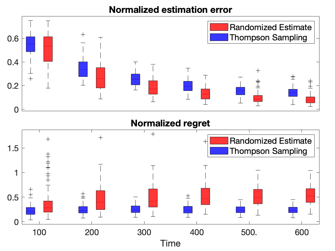
Figure 2: The performance of Algorithm 2 (blue) compared to Randomized Estimate policy (red) [2] for flight control of X-29A airplane. The top box-plots are for the normalized squared estimation error, ${\left|\kern-1.29167pt\left|\boldsymbol{\widehat{\theta}_{n}}-\boldsymbol{\theta_{0}}\right|\kern-1.29167pt\right|}^{2}$ divided by $p(p+q)\boldsymbol{\tau}_{n}^{-1/2}\log\boldsymbol{\tau}_{n}$, at times 100, 200, 300, 400, 500, and 600 for $100$ replications. Similarly, the lower graph showcases the distribution of the regret $\mathrm{Reg}\left(T\right)$, normalized by $p(p+q)T^{1/2}\log T$.

Figure 2 depicts the box plot corresponding to Figure 1 that is for the flight control of X-29A airplane at 2000 ft. In the following experiments, we keep the setting given in Section 6 for the cost and noise covariance matrices, and compare Algorithm 2 to Randomized Estimate policy [2].

Next, the empirical results of the flight control problem in Boeing 747 airplane at 20000 ft altitude are provided [43]. The true drift matrices of the Boeing 747 are

$$A_{0}=\begin{bmatrix}-0.199\;&0.003\;&-0.980\;&0.038\\ -3.868\;&-0.929\;&0.471\;&-0.008\\ 1.591\;&-0.015\;&-0.309\;&0.003\\ -0.198\;&0.958\;&0.021\;&0.000\end{bmatrix},~{}~{}~{}~{}B_{0}=\begin{bmatrix}-0.001\;&0.058\\ 0.296\;&0.153\\ 0.012\;&-0.908\\ 0.015\;&0.008\end{bmatrix}.$$

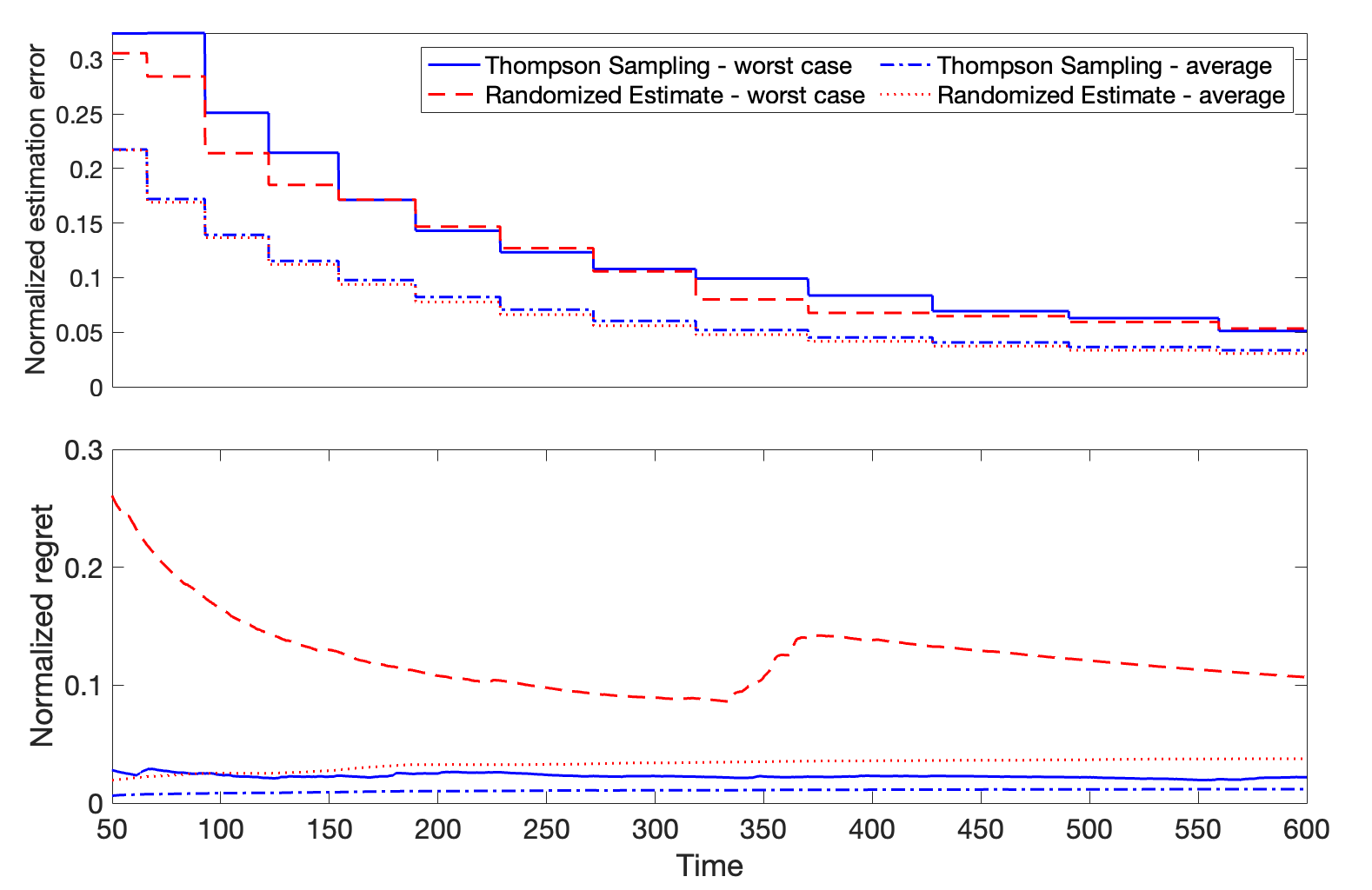
Figure 3: The performance of Algorithm 2 (blue) compared to Randomized Estimate policy (red) [2] for the flight control of Boeing 747 airplane. The top graph plots the normalized squared estimation error, ${\left|\kern-1.29167pt\left|\boldsymbol{\widehat{\theta}_{n}}-\boldsymbol{\theta_{0}}\right|\kern-1.29167pt\right|}^{2}$ divided by $p(p+q)\boldsymbol{\tau}_{n}^{-1/2}\log\boldsymbol{\tau}_{n}$, for $100$ replications. Similarly, the lower graph showcases the regret $\mathrm{Reg}\left(T\right)$, normalized by $p(p+q)T^{1/2}\log T$.

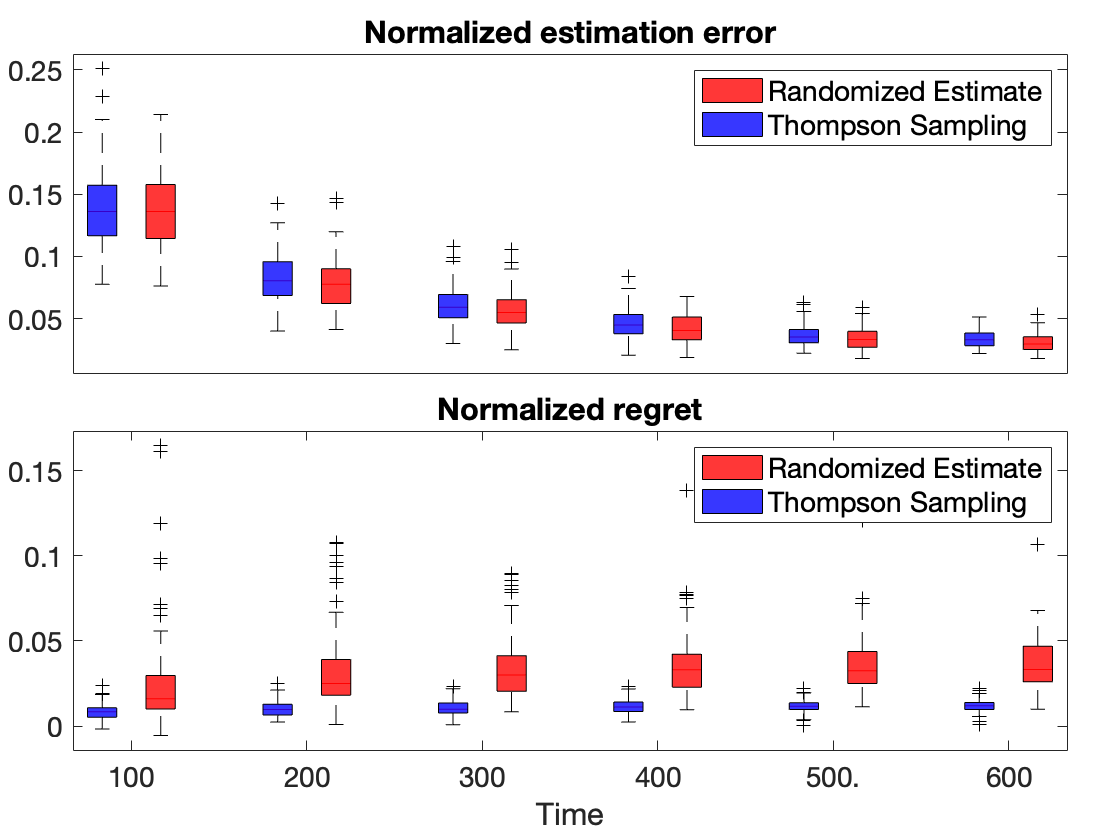
Figure 4: The performance of Algorithm 2 (blue) compared to Randomized Estimate policy (red) [2] for the flight control of Boeing 747 airplane. The top graph plots the normalized squared estimation error, ${\left|\kern-1.29167pt\left|\boldsymbol{\widehat{\theta}_{n}}-\boldsymbol{\theta_{0}}\right|\kern-1.29167pt\right|}^{2}$ divided by $p(p+q)\boldsymbol{\tau}_{n}^{-1/2}\log\boldsymbol{\tau}_{n}$, at times 100, 200, 300, 400, 500, and 600 for $100$ replications. Similarly, the lower graph showcases the regret $\mathrm{Reg}\left(T\right)$, normalized by $p(p+q)T^{1/2}\log T$.

Then, the blood glucose control problem is studied [47, 50]. The true drift matrices are

$$A_{0}=\begin{bmatrix}1.91\;&-2.82\;&0.91\\ 1.00\;&-1.00\;&0.00\\ 0.00\;&1.00\;&-1.00\end{bmatrix},~{}~{}~{}~{}B_{0}=\begin{bmatrix}-0.0992\\ 0.0000\\ 0.0000\end{bmatrix}.$$

Note that from a practical point of view, worst-case behavior are of crucial importance in this problem.

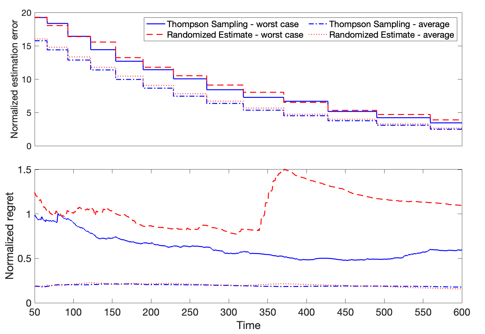
Figure 5: The performance of Algorithm 2 (blue) compared to Randomized Estimate policy (red) [2] for the the blood glucose control. The top graph plots the normalized squared estimation error, ${\left|\kern-1.29167pt\left|\boldsymbol{\widehat{\theta}_{n}}-\boldsymbol{\theta_{0}}\right|\kern-1.29167pt\right|}^{2}$ divided by $p(p+q)\boldsymbol{\tau}_{n}^{-1/2}\log\boldsymbol{\tau}_{n}$, for $100$ replications. Similarly, the lower graph showcases the regret $\mathrm{Reg}\left(T\right)$, normalized by $p(p+q)T^{1/2}\log T$.

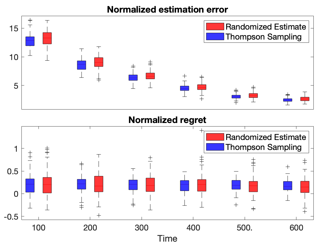
Figure 6: The performance of Algorithm 2 (blue) compared to Randomized Estimate policy (red) [2] for the the blood glucose control. The top graph plots the normalized squared estimation error, ${\left|\kern-1.29167pt\left|\boldsymbol{\widehat{\theta}_{n}}-\boldsymbol{\theta_{0}}\right|\kern-1.29167pt\right|}^{2}$ divided by $p(p+q)\boldsymbol{\tau}_{n}^{-1/2}\log\boldsymbol{\tau}_{n}$, at times 100, 200, 300, 400, 500, and 600 for $100$ replications. Similarly, the lower graph showcases the regret $\mathrm{Reg}\left(T\right)$, normalized by $p(p+q)T^{1/2}\log T$.

References

• [1] W. R. Thompson, “On the likelihood that one unknown probability exceeds another in view of the evidence of two samples,” Biometrika, vol. 25, no. 3/4, pp. 285–294, 1933.
• [2] M. K. S. Faradonbeh and M. S. S. Faradonbeh, “Efficient estimation and control of unknown stochastic differential equations,” arXiv preprint arXiv:2109.07630, 2021.
• [3] P. A. Ioannou and J. Sun, Robust adaptive control.   PTR Prentice-Hall Upper Saddle River, NJ, 1996, vol. 1.
• [4] F. L. Lewis, L. Xie, and D. Popa, Optimal and robust estimation: with an introduction to stochastic control theory.   CRC press, 2017.
• [5] A. Subrahmanyam and G. P. Rao, Identification of Continuous-time Systems: Linear and Robust Parameter Estimation.   CRC Press, 2019.
• [6] J. Umenberger, M. Ferizbegovic, T. B. Schön, and H. Hjalmarsson, “Robust exploration in linear quadratic reinforcement learning,” Advances in Neural Information Processing Systems, vol. 32, 2019.
• [7] S. Agrawal and N. Goyal, “Analysis of thompson sampling for the multi-armed bandit problem,” in Conference on learning theory.   JMLR Workshop and Conference Proceedings, 2012, pp. 39–1.
• [8] ——, “Further optimal regret bounds for thompson sampling,” in Artificial intelligence and statistics.   PMLR, 2013, pp. 99–107.
• [9] A. Gopalan and S. Mannor, “Thompson sampling for learning parameterized markov decision processes,” in Conference on Learning Theory.   PMLR, 2015, pp. 861–898.
• [10] M. J. Kim, “Thompson sampling for stochastic control: The finite parameter case,” IEEE Transactions on Automatic Control, vol. 62, no. 12, pp. 6415–6422, 2017.
• [11] M. Abeille and A. Lazaric, “Linear thompson sampling revisited,” in Artificial Intelligence and Statistics.   PMLR, 2017, pp. 176–184.
• [12] N. Hamidi and M. Bayati, “On worst-case regret of linear thompson sampling,” arXiv preprint arXiv:2006.06790, 2020.
• [13] D. Russo and B. Van Roy, “Learning to optimize via posterior sampling,” Mathematics of Operations Research, vol. 39, no. 4, pp. 1221–1243, 2014.
• [14] ——, “An information-theoretic analysis of thompson sampling,” The Journal of Machine Learning Research, vol. 17, no. 1, pp. 2442–2471, 2016.
• [15] D. Russo, B. Van Roy, A. Kazerouni, I. Osband, and Z. Wen, “A tutorial on thompson sampling,” arXiv preprint arXiv:1707.02038, 2017.
• [16] M. Abeille and A. Lazaric, “Improved regret bounds for thompson sampling in linear quadratic control problems,” in International Conference on Machine Learning.   PMLR, 2018, pp. 1–9.
• [17] Y. Ouyang, M. Gagrani, and R. Jain, “Posterior sampling-based reinforcement learning for control of unknown linear systems,” IEEE Transactions on Automatic Control, vol. 65, no. 8, pp. 3600–3607, 2019.
• [18] M. K. S. Faradonbeh, A. Tewari, and G. Michailidis, “Finite-time adaptive stabilization of linear systems,” IEEE Transactions on Automatic Control, vol. 64, no. 8, pp. 3498–3505, 2018.
• [19] ——, “Randomized algorithms for data-driven stabilization of stochastic linear systems,” in 2019 IEEE Data Science Workshop (DSW).   IEEE, 2019, pp. 170–174.
• [20] ——, “On applications of bootstrap in continuous space reinforcement learning,” in 2019 IEEE 58th Conference on Decision and Control (CDC).   IEEE, 2019, pp. 1977–1984.
• [21] ——, “On adaptive linear–quadratic regulators,” Automatica, vol. 117, p. 108982, 2020.
• [22] ——, “Input perturbations for adaptive control and learning,” Automatica, vol. 117, p. 108950, 2020.
• [23] ——, “Optimism-based adaptive regulation of linear-quadratic systems,” IEEE Transactions on Automatic Control, vol. 66, no. 4, pp. 1802–1808, 2020.
• [24] S. Sudhakara, A. Mahajan, A. Nayyar, and Y. Ouyang, “Scalable regret for learning to control network-coupled subsystems with unknown dynamics,” arXiv preprint arXiv:2108.07970, 2021.
• [25] P. Mandl, “Consistency of estimators in controlled systems,” in Stochastic Differential Systems.   Springer, 1989, pp. 227–234.
• [26] T. E. Duncan and B. Pasik-Duncan, “Adaptive control of continuous-time linear stochastic systems,” Mathematics of Control, signals and systems, vol. 3, no. 1, pp. 45–60, 1990.
• [27] P. Caines, “Continuous time stochastic adaptive control: non-explosion, $\varepsilon$-consistency and stability,” Systems & control letters, vol. 19, no. 3, pp. 169–176, 1992.
• [28] T. E. Duncan, L. Guo, and B. Pasik-Duncan, “Adaptive continuous-time linear quadratic gaussian control,” IEEE Transactions on automatic control, vol. 44, no. 9, pp. 1653–1662, 1999.
• [29] P. E. Caines and D. Levanony, “Stochastic $\varepsilon$-optimal linear quadratic adaptation: An alternating controls policy,” SIAM Journal on Control and Optimization, vol. 57, no. 2, pp. 1094–1126, 2019.
• [30] S. A. A. Rizvi and Z. Lin, “Output feedback reinforcement learning control for the continuous-time linear quadratic regulator problem,” in 2018 Annual American Control Conference (ACC).   IEEE, 2018, pp. 3417–3422.
• [31] K. Doya, “Reinforcement learning in continuous time and space,” Neural computation, vol. 12, no. 1, pp. 219–245, 2000.
• [32] H. Wang, T. Zariphopoulou, and X. Y. Zhou, “Reinforcement learning in continuous time and space: A stochastic control approach.” J. Mach. Learn. Res., vol. 21, pp. 198–1, 2020.
• [33] Z.-P. Jiang, T. Bian, and W. Gao, “Learning-based control: A tutorial and some recent results,” Foundations and Trends® in Systems and Control, vol. 8, no. 3, 2020.
• [34] M. Basei, X. Guo, A. Hu, and Y. Zhang, “Logarithmic regret for episodic continuous-time linear-quadratic reinforcement learning over a finite-time horizon,” Available at SSRN 3848428, 2021.
• [35] L. Szpruch, T. Treetanthiploet, and Y. Zhang, “Exploration-exploitation trade-off for continuous-time episodic reinforcement learning with linear-convex models,” arXiv preprint arXiv:2112.10264, 2021.
• [36] M. K. S. Faradonbeh and M. S. S. Faradonbeh, “Bayesian algorithms learn to stabilize unknown continuous-time systems,” arXiv preprint arXiv:2112.15094, 2021.
• [37] I. Karatzas and S. Shreve, Brownian motion and stochastic calculus.   Springer Science & Business Media, 2012, vol. 113.
• [38] G. Chen, G. Chen, and S.-H. Hsu, Linear stochastic control systems.   CRC press, 1995, vol. 3.
• [39] J. Yong and X. Y. Zhou, Stochastic controls: Hamiltonian systems and HJB equations.   Springer Science & Business Media, 1999, vol. 43.
• [40] H. Pham, Continuous-time stochastic control and optimization with financial applications.   Springer Science & Business Media, 2009, vol. 61.
• [41] S. P. Bhattacharyya and L. H. Keel, Linear Multivariable Control Systems.   Cambridge University Press, 2022.
• [42] J. T. Bosworth, Linearized aerodynamic and control law models of the X-29A airplane and comparison with flight data.   National Aeronautics and Space Administration, Office of Management …, 1992, vol. 4356.
• [43] T. Ishihara, H.-J. Guo, and H. Takeda, “A design of discrete-time integral controllers with computation delays via loop transfer recovery,” Automatica, vol. 28, no. 3, pp. 599–603, 1992.
• [44] P. Cheridito, H. M. Soner, and N. Touzi, “Small time path behavior of double stochastic integrals and applications to stochastic control,” The Annals of Applied Probability, vol. 15, no. 4, pp. 2472–2495, 2005.
• [45] B. Laurent and P. Massart, “Adaptive estimation of a quadratic functional by model selection,” Annals of Statistics, pp. 1302–1338, 2000.
• [46] J. A. Tropp, “User-friendly tail bounds for sums of random matrices,” Foundations of computational mathematics, vol. 12, no. 4, pp. 389–434, 2012.
• [47] T. Zhou, J. L. Dickson, and J. Geoffrey Chase, “Autoregressive modeling of drift and random error to characterize a continuous intravascular glucose monitoring sensor,” Journal of Diabetes Science and Technology, vol. 12, no. 1, pp. 90–104, 2018.
• [48] P. Hartman and A. Wintner, “The spectra of toeplitz’s matrices,” American Journal of Mathematics, vol. 76, no. 4, pp. 867–882, 1954.
• [49] L. Reichel and L. N. Trefethen, “Eigenvalues and pseudo-eigenvalues of toeplitz matrices,” Linear algebra and its applications, vol. 162, pp. 153–185, 1992.
• [50] R. Gondhalekar, E. Dassau, and F. J. Doyle III, “Periodic zone-mpc with asymmetric costs for outpatient-ready safety of an artificial pancreas to treat type 1 diabetes,” Automatica, vol. 71, pp. 237–246, 2016.