A black hole x-ray binary (XRB) system forms when gas is stripped from a normal star and accretes onto a black hole, which heats the gas sufficiently to emit x-rays. We report a polarimetric observation of the XRB Cygnus X-1 using the Imaging x-ray Polarimetry Explorer. The electric field position angle aligns with the outflowing jet, indicating that the jet is launched from the inner x-ray emitting region. The polarization degree is $\mathbf{4.01\pm 0.20\%}$ at 2 to 8 kiloelectronvolts, implying that the accretion disk is viewed closer to edge-on than the binary orbit. The observations reveal that hot x-ray emitting plasma is spatially extended in a plane perpendicular to the jet axis, not parallel to the jet.

Cygnus X-1 (Cyg X-1, also catalogued as HD 226868) is a bright and persistent x-ray source. It is a binary system containing a 21.2$\pm 2.2$ solar-mass black hole in a 5.6 day orbit with a 40.6${}^{+7.7}_{-7.1}$ solar-mass star and is located at a distance of 2.22${}^{+0.18}_{-0.17}$ kiloparsecs (kpc)  (?). Gas is stripped from the companion star; as it falls in the strong gravitational field of the black hole it forms an accretion disk that is heated to millions of kelvin. The hot incandescent gas emits x-rays. Previous analyses of the thermal x-ray flux, its energy spectrum, and the shape of the x-ray emission lines have indicated that the black hole in Cyg X-1 spins rapidly, with a dimensionless spin parameter $a>0.92$ (close to the maximum possible value of 1)  (?). Cyg X-1 also produces two pencil-shaped outflows of magnetized plasma, called jets, that have been imaged in the radio band  (?). It is thus classified as a microquasar, being analogous to much larger radio-loud quasars, supermassive black holes with jets.

Black hole x-ray binaries are observed in states of x-ray emission thought to correspond to different configurations of the accreting matter  (?). In the soft state, the x-rays are dominated by thermal emission from the accretion disk. The thermal emission is expected to be polarized because x-rays scatter off electrons in the accretion disk  (?, ?, ?). In the hard state, the x-ray emission is produced by single and multiple scatterings of photons (coming from the accretion disk or generated by electrons in the magnetic field) off electrons of hot coronal gas. Observations constrain the corona to be much hotter ($k\,T_{\rm e}\sim$100 keV, with $k$ being the Boltzmann constant and $T_{\rm e}$ the electron temperature) than the accretion disk ($k\,T_{\rm d}\sim 0.1$ keV). The shape of the corona, and its location with respect to the accretion disk, are a matter of debate  (?, ?), but can be constrained by x-ray polarimetry  (?). Reflection of x-rays emitted by the corona off the accretion disk produces an emission component that includes the iron K$\alpha$ fluorescence line at $\sim 6.4$ keV, which can constrain the velocity of the accretion disk gas orbiting the black hole and the time dilation close to the black hole. The reflection component is also expected to be polarized  (?, ?).

We report here on x-ray polarimetric observations of Cyg X-1 with the Imaging X-ray Polarimetry Explorer (IXPE) space telescope  (?). Theoretical predictions of the Cyg X-1 polarization degree (in the 2–8 keV IXPE band) are around 1% or lower, depending on the emission state  (?, ?, ?, ?). These expectations used an inclination angle (the angle between the black hole spin axis and the line of sight) of $i=27\mbox{$.\!\!^{\circ}$}5\pm 0\mbox{$.\!\!^{\circ}$}8$ inferred from optical observations of the binary system  (?). Earlier polarization observations with the OSO-8 gave polarization degree 2.44$\pm$1.07% and polarization angle (measured on the plane of the sky from north to east) $-18\hbox{${}^{\circ}$}\pm 13\hbox{${}^{\circ}$}$ at 2.6 keV  (?, ?) and a non-detection at higher energies  (?). IXPE observed Cyg X-1 from 2022 May 15 to 21 with an exposure time of $\sim$242 ksec. The IXPE 2–8 keV observations were coordinated with simultaneous x-ray and gamma-ray observations covering the energy range 0.2–250 keV, including the Neutron Star Interior Composition Explorer Mission (NICER, 0.2–12 keV), the Nuclear Spectroscopic Telescope Array (NuSTAR, 3–79 keV), the Swift X-ray Telescope (XRT, 0.2–10 keV), the Astronomical Roentgen Telescope – X-ray Concentrator (ART-XC, 4–30 keV) of the Spectrum-Röntgen-Gamma observatory (SRG), and the INTEGRAL Soft Gamma-Ray Imager (ISGRI, 30–80 keV) on the International Gamma-Ray Astrophysics Laboratory (INTEGRAL) space telescopes  (?). Simultaneous optical observations were performed with the Double Image Polarimeter 2 (DIPol-2) polarimeter mounted on the Tohoku 60 cm telescope at the Haleakala Observatory and the Robotic Polarimeter (RoboPol) at the 1.3 m telescope of the Skinakas observatory, Greece  (?).

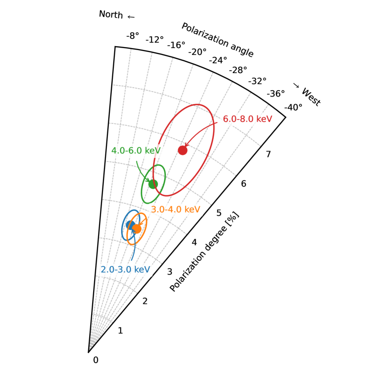
Figure 1: Energy-dependent x-ray polarization of Cyg X-1. Polarization degree and polarization angle, derived from the IXPE observations, in four energy bands (labeled in different colours). The ellipses denote the 68.3% confidence regions.

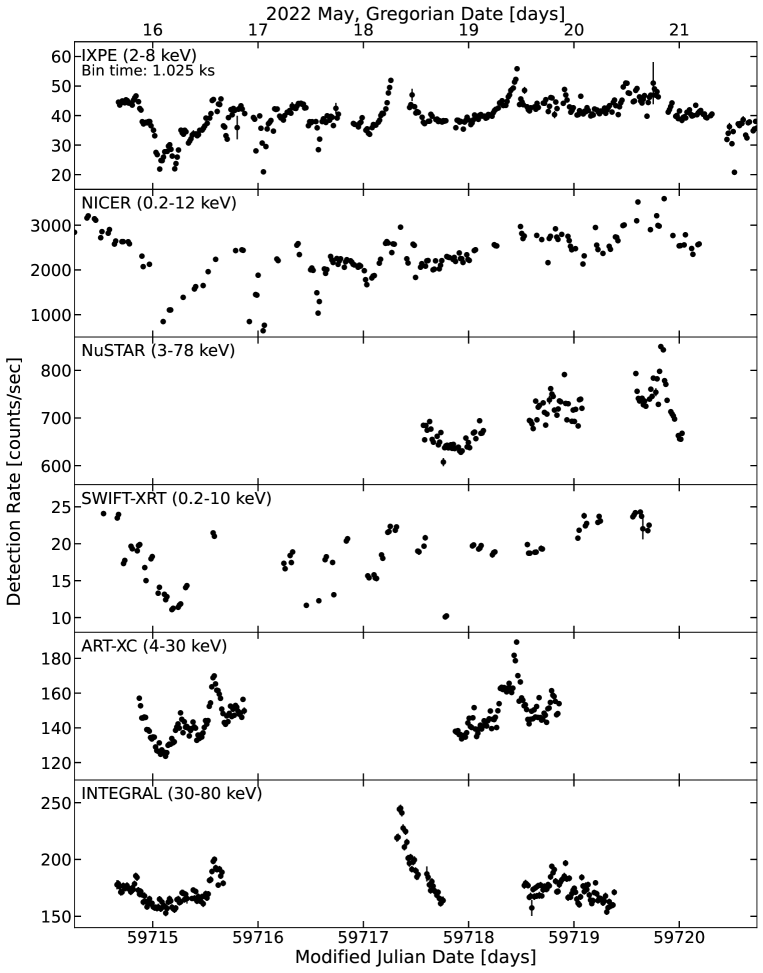
Figure S1: X-ray light curves of Cyg X-1 from the 2022 May 15 to 21 observation campaign. From top to bottom: the IXPE, NICER, NuSTAR, Swift/XRT, SRG/ART-XC, and INTEGRAL light curves.

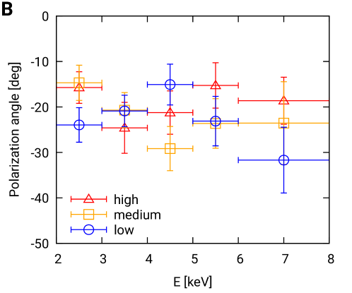
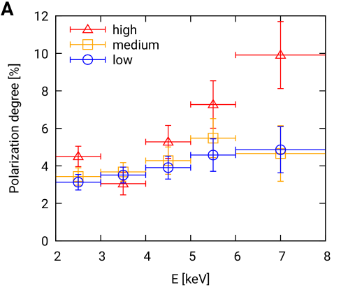
Figure S6: Polarization of Cyg X-1 at different flux levels. Comparison of the polarization degree (A) and polarization angle (B) for three different flux selected data sets.

During the observation campaign Cyg X-1 was highly variable over the entire 0.2–250 keV energy range (Figure S1). The source was in the hard x-ray state with a photon index of 1.6 (Table Optical polarimetry) and a 0.2–250 keV luminosity of 1.1% of the Eddington luminosity (the luminosity at which the radiation pressure on electrons equals the gravitational pull on the ions of the accreted material). We detected linear polarization in the IXPE data with a $>20\sigma$ statistical confidence (Figures 1,S3). The 2–8 keV polarization degree is $4.01\pm 0.20$% at an electric field position angle of $-20\mbox{$.\!\!^{\circ}$}7\pm 1\mbox{$.\!\!^{\circ}$}4$. The polarization degree and angle are consistent with the previous results of OSO-8 at 2.6 keV  (?). The evidence for an increase of the polarization degree with energy (Figures 1, S5) is significant on the 3.4 $\sigma$ level  (?). We find a 2.4$\sigma$ indication that the polarization degree increases with the source flux (Figure S6).

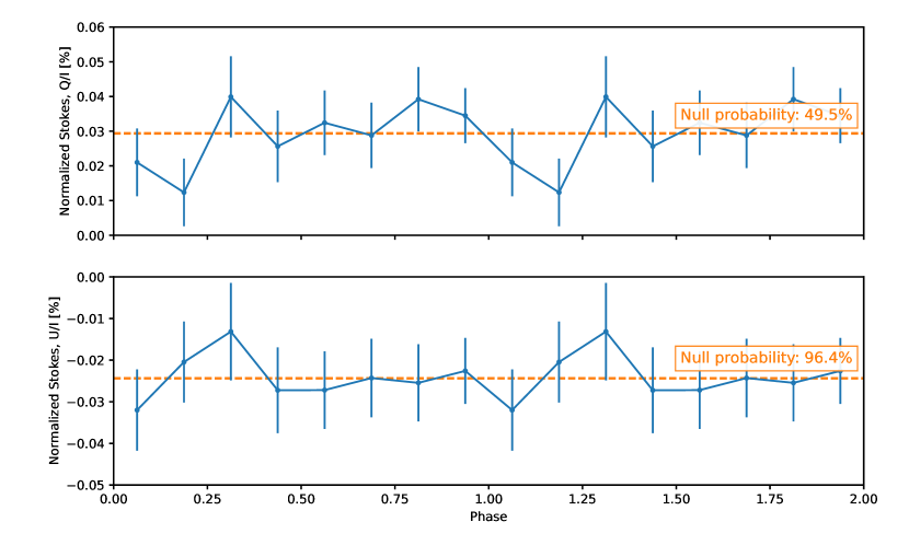
Figure S7: Orbital phase dependence of the Cyg X-1 x-ray polarization properties. The observed x-ray normalized Stokes parameters $Q/I$ and $U/I$ (summed from 2 to 8 keV) are statistically consistent with being constant as a function of the orbital phase. Note that the results are shown for two orbital periods. The orbital phase of 0 corresponds to the superior conjunction maximizing the stellar wind absorption of the x-rays.

We find no evidence that the polarization properties depend on orbital phase of the binary system (Figure S7). This excludes the possibility that the observed x-ray polarization originates from the scattering of x-ray photons off the companion star or its wind, and shows that these effects do not measurably impact the polarization properties.

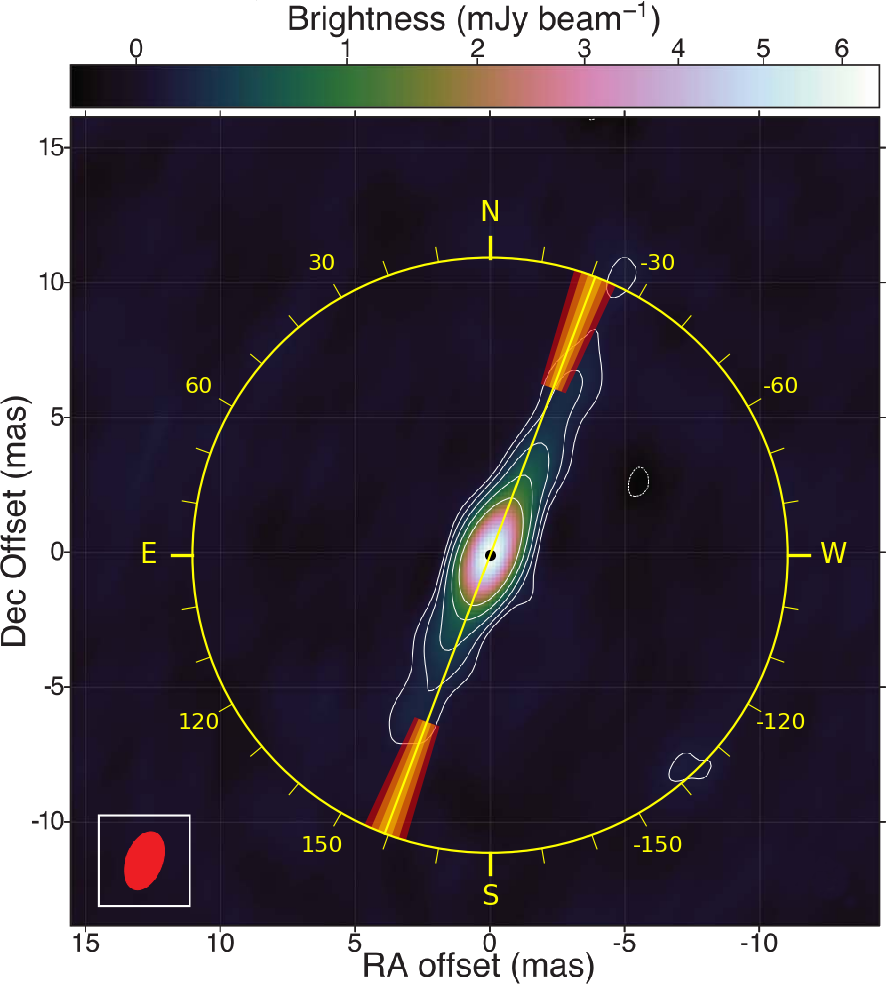
Figure 2: Comparison of the x-ray polarization direction with the radio jet  (?). The 2–8 keV electric vector position angle is shown with the yellow line, and the one, two and three sigma confidence intervals are given by the orange to red regions. We infer (see text) that most x-rays are emitted by a $\sim$2,000 km diameter region surrounding the $\sim$60 km diameter black hole, far smaller than the resolution of the radio image (indicated by the red ellipse). The coordinate offsets in right ascension (RA) and declination (Dec) are in the J2000 equinox in units of milli-arcseconds (mas) with 1 arcsecond being 1/3600^th of a degree. The color scale shows the radio flux in milli-Jansky with 1 Jansky being $10^{-26}$ W m^-2 Hz ^-1.

We calculated a suite of emission models and compared them to the observations  (?). We estimate that $>90$% of the x-rays come from the inner $\sim$2,000 km diameter region surrounding the $\sim$60 km diameter black hole. We compare the orientation of the x-ray bright region (which we assume is determined by the x-ray polarization angle; Figure 3) to the orientation of the billion-km-scale radio jet. We find that the x-ray polarization aligns with the radio jet to within $\sim$5^∘ (Figure 2).

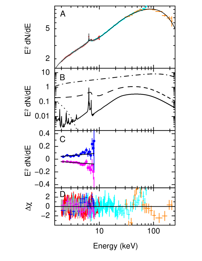
Figure S8: Results of spectropolarimetric fitting. (A) NICER (red), NuSTAR (cyan), IXPE (grey) and INTEGRAL/ISGRI (orange) Stokes $I$ spectrum unfolded around the best-fit model (black solid line). For each bin of the energy spectrum, the unfolded data point is the number of observed counts times the best-fit model value divided by the counts expected in the bin for the best-fit model. For plotting purposes only, data and model are both divided by the relevant mbpo model to remove calibration discrepancies. The specific photon flux $dN/dE$ has units of photons cm^-2 s^-1 keV^-1. (B) Individual components of the best-fit model: thermal disk emission (dotted line), Compton scattered emission from the corona (dashed dotted line), relativistic reflection (dashed line), non-relativistic reflection (solid line). (C) Stokes $Q$ (blue circles) and $U$ (magenta squares), also unfolded around the best-fit model. (D) Residuals (contributions to $\chi$). For plotting purposes only, data from different detectors of the same observatory have been grouped together, and a maximum of 10 energy channels have been grouped together to achieve a signal-to-noise ratio of 150.

We decomposed the broadband energy spectra observed simultaneously with IXPE, NICER, NuSTAR, and INTEGRAL into a multi-temperature black body component (thermal emission from the accretion disk), a power-law component (from multiple Compton scattering events in the corona), emission reflected off the accretion disk, and emission from more distant stationary plasma  (?) (Figure S8). We find that the coronal emission strongly dominates in the IXPE energy band, contributing $\sim 90$% of the observed flux. The accretion disk and reflected emission components contribute $<$1% and $\sim$10% of the emission, respectively. Therefore our polarization measurements are likely to be dominated by the coronal emission.

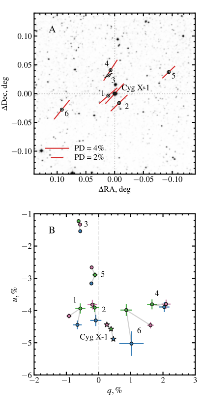
Figure S11: Polarization of nearby field stars around Cyg X-1. (A) Polarization vectors of the field stars (open circles) and Cyg X-1 (filled circle) in the $B$-filter, with field stars image as a background. The length of the solid lines is proportional to the polarization degree. The deviations in declination ($\Delta$Dec) and right ascension ($\Delta$RA) are relative to the Cyg X-1 position (grey dotted lines). (B) The observed normalized Stokes parameters $q$ and $u$ for the field stars (circles) and Cyg X-1 (stars). Blue, green and magenta colors correspond to $B$, $V$, and $R$ filters, respectively. For clarity, the grey solid lines connect the $B$, $V$, and $R$ results for each source. Uncertainties are 1$\sigma$. The vertical grey dashed line indicates the $q=0$ axis. Stars Ref 1 and Ref 2 are chosen as the IS polarization standards.

We analyzed the optical data in various wavelengths  (?), finding an intrinsic optical polarization degree of $\sim$1% and polarization angle of $-24\hbox{${}^{\circ}$}$. The uncertainties on these results are dominated by systematic effects related to the choice of polarization reference stars and are $\pm$0.1% on the polarization degree and $\pm 13\hbox{${}^{\circ}$}$ on the polarization direction (Figures S11-S12, and Table S4). The optical polarization direction is thought to indicate the orientation of the orbital axis projected onto the sky  (?). We find it aligns with the x-ray polarization direction and the radio jet.

The alignment of the x-ray polarization with the radio jet indicates that the inner x-ray emitting region is directly related to the radio jet. If the x-ray polarization is perpendicular to the inner accretion disk plane, as favored in our models  (?), this implies that the inner accretion disk is perpendicular to the radio jet, at least on the plane of the sky. This is consistent with the hypothesis that jets of microquasars (and, by extension, of quasars) are launched perpendicular to the inner accretion flow  (?).

Figure 3 compares our observed polarization with theoretical predictions made using models of the corona  (?). We find that the only models that are consistent with the observations are those in which the coronal plasma is extended perpendicular to the jet axis, so probably parallel to the accretion disk. In these models, repeated scatterings in the plane of the corona polarize the x-rays perpendicular to that plane. Two models are consistent with our observations: i) a hot corona sandwiching the accretion disk  (?), as predicted by numerical accretion disk simulations  (?) or ii) a composite accretion flow with a truncated cold, geometrically thin optically thick disk and an inner, geometrically thick but optically thin, laterally extended region of hot plasma, possibly produced by evaporation of the cold disk  (?). If the jet is launched from the inner, magnetized region of the disk, the jet carrying away disk angular momentum could leave behind a radially extended hot and optically thin corona  (?).

The polarization data rule out models in which the corona is a narrow plasma column or cone along the jet axis, or consists of two compact regions above and below the black hole. Our modeling of these scenarios accounts for the effect of the coronal emission reflecting off the accretion disk  (?). These models predict polarization degree well below the observed values. Models that produce high polarization degree predict polarization directions close to perpendicular to the jet axis, a decreasing polarization degree with energy, or both, and therefore disagree with the observations.

In our favored corona models, the high polarization degree we observe requires that the x-ray bright region is seen at a higher inclination than the $\sim$27^∘ inclination of the binary orbit. Sandwich corona models involving the Compton scattering of disk photons with initial energies of $\sim 0.1$ keV require inclinations exceeding 65^∘. Truncated disk models invoking Compton scattering of disk or internally generated lower-energy ($\sim$1–10 eV) synchrotron photons  (?) can reproduce the observed polarization degree for inclinations $>$45^∘. Compared to the models with disk photons, the larger number of scatterings required to energize lower-energy synchrotron photons to keV energies results in higher polarization degree in the IXPE energy band (Figure S9)  (?).

Although the x-ray polarization, optical polarization, and radio jet approximately align in the plane of the sky, the inclination of the x-ray bright region exceeds that of the binary orbit, implying that the inner accretion flow is seen more edge on than the binary orbit. Because the bodies of a stellar system typically orbit and spin around the same axis (as most planets in our solar system), we consider potential explanations for the mismatch between the inner accretion disk inclination and the orbital inclination.

Stellar mass black holes are formed during supernovae. The supernova that occurred in Cyg X-1 might have left the black hole with a misaligned spin. Gravitational effects could align the inner accretion flow angular momentum vector with the black hole spin vector  (?). In this scenario, aligning the inner accretion disk angular momentum vector with the black hole spin vector would also align the radio jet produced by the inner accretion disk with the black hole spin vector. Several, but not all, analyses of Cyg X-1 reflected emission spectra give inclinations consistent with our $i>45^{\circ}$ constraint  (?, ?).

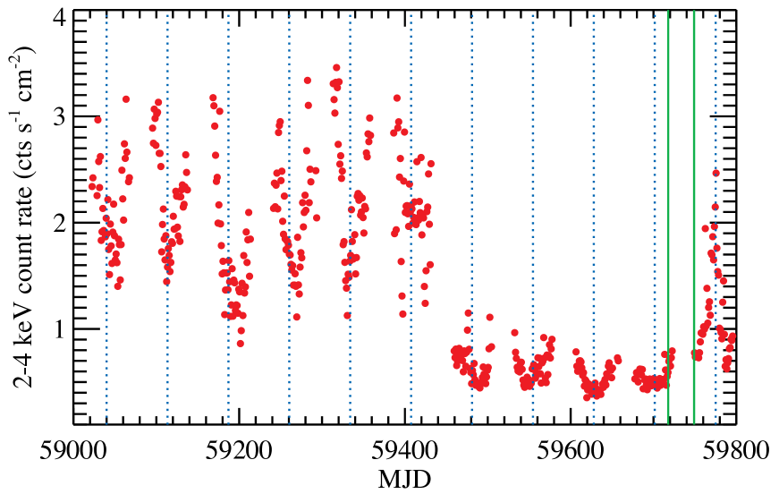
Figure S2: Long-term Cyg X-1 x-ray light curve. The figure shows the daily 2–4 keV count rate obtained from the MAXI monitor from May 31, 2020 (MJD 59000) to August 9, 2022 (MJD 59800). Phases of high 2–4 keV fluxes during the soft state and low 2–4 keV fluxes during the hard state can be recognized. The vertical dotted lines (blue) show the dates of the superorbital flux minima, appearing at ${\rm MJD}=59040.0+73.5n$, with $n$ being an integer number. The two vertical solid lines (green) show the mid-times of two IXPE campaigns, 2022 May 15 to 21 and June 18 to 20, respectively. The first observation was close to the superorbital flux minimum, and the second was shifted by about half-period. The second observation was taken right before the short incursion into the soft state.

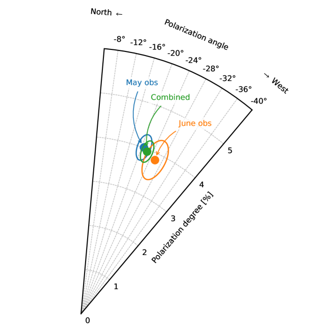
Figure S4: Linear x-ray polarization of Cyg X-1 measured in two occasions, as well as the combined result. The figure shows the polarization degree and angle of the 2022 May 15 to 21 observations (blue), the 2022 June 18 to 20 observations (orange), and for the combined data set (green). For each result the most likely values (circles) and 68.3% confidence regions (ellipses) are shown.

An alternative explanation for the large inclination of the x-ray emitting region invokes the precession of the inner accretion flow with a period of much longer than the orbital period  (?). From our analysis of a 2–4 keV long-term x-ray light-curve we infer that the IXPE observations were performed close to the maximum inner disk inclination (Figure S2)  (?). We tested the hypothesis that the inner flow precesses with an amplitude of ${}^{>}_{\sim}17\mbox{$.\!\!^{\circ}$}5$ by performing an additional 86 ksec IXPE target of opportunity observation of Cyg X-1 from 2022 June 18 to 20, 33 days after the May observations, which corresponds to half of the current superorbital period  (?). If this hypothesis is correct, we expected the polarization degree to drop from 4.01$\pm$0.20% to $\ll$1% due to the inclination changing from $i>45\hbox{${}^{\circ}$}$ in May to $i\lesssim 10\hbox{${}^{\circ}$}$ in June. The observations showed the source in the same hard state with a 2–8 keV polarization degree and angle of $3.84\pm 0.31$% and $-25\mbox{$.\!\!^{\circ}$}7\pm 2\mbox{$.\!\!^{\circ}$}3$, respectively (Figure S4)  (?). The polarization degree thus stayed constant between the May and June observations within the statistical uncertainties of the observations. We therefore disfavor the hypothesis that precession of the inner accretion flow leads to the high polarization degree of the May observation. The combined May and June polarization degree and angle are $3.95\pm 0.17$% and $-22\mbox{$.\!\!^{\circ}$}2\pm 1\mbox{$.\!\!^{\circ}$}2$, respectively (Figure S4)  (?).

Several authors noted that optically thin synchrotron emission from the base of the jet could contribute up to 5% to the Cyg X-1 x-ray emission in the hard state  (?, ?). Synchrotron emission from electrons gyrating around magnetic field lines is polarized perpendicular to those field lines. Our observation of the x-rays being polarized parallel to the jet axis would require synchrotron emission from a toroidal magnetic field wound around the jet axis. For this magnetic field geometry seen at an inclination of $27\mbox{$.\!\!^{\circ}$}5$ the theoretical upper limit on the polarization degree of the synchrotron emission is 8%  (?). The jet thus contributes $<0.4\%$ of the observed polarization degree. Furthermore, if the almost constant jet emission was the main source of the observed polarization, we would expect that a rise in the x-ray flux from the inner accretion flow would lead to an overall smaller polarization degree – contrary to the observed trend (Figure S6).

To summarize: the polarized x-rays from the immediate surrounding of the black hole carry the imprint of the geometry of the emitting gas. We find that the x-ray bright plasma is extended perpendicular to the radio jet. The high observed polarization degree either implies a more edge-on viewing geometry than given by the optical data, or yet unknown physical effects responsible for production of the x-rays in accreting black hole systems.

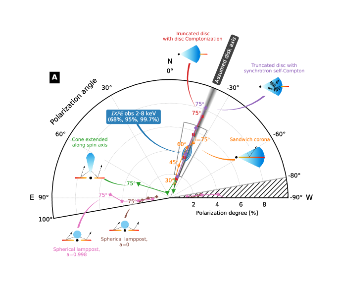
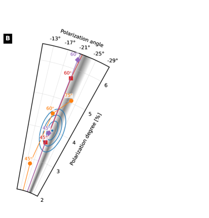
Figure 3: Comparison of the observed 2–8 keV polarization degree and angle with model predictions. (A) The blue dot shows the polarization degree and angle, with the blue ellipses indicating the the 68%, 95% and 99.7% confidence levels (equivalent to 1$\sigma$, 2$\sigma$ and 3$\sigma$). Model predictions assume that the inner disk spin axis has position angle of $-22\hbox{${}^{\circ}$}$ (consistent with the radio jet), and that the inner disk angular momentum vector points away from the observer (as does the orbital angular momentum vector)  (?). The grey band shows the uncertainty of the radio jet orientation; we adopt this as the uncertainty of the disk spin axis in all models. Each colored line shows the results of each chosen one corona geometry, with symbols indicating different values as a function of the inner disk inclination $i$. Inset diagrams depict the assumed black hole (black), corona (blue), and accretion disk (orange-red) configurations. Black arrows indicate photon paths. Models with coronae extending parallel to the inner accretion disk can match the IXPE observations, but coronae located or extending along the spin axis of the inner accretion disk cannot. The position angles are shown from $-80\hbox{${}^{\circ}$}$ to +100^∘ (instead of $-90\hbox{${}^{\circ}$}$ to +90^∘) to show more clearly the models straddling the $\pm 90\hbox{${}^{\circ}$}$ borders. (B) A zoom into the region around the measured value, marked with the grey box in panel A.

Acknowledgements: The authors thank James Miller-Jones, Jerome Orosz and Andrzej Zdziarski for very helpful discussions of the optical constraints on the orbital inclination of Cyg X-1 and optical position angles. We are grateful to three anonymous referees whose excellent comments contributed to strengthening the paper. The authors thank Tom Maccarone for emphasizing that stellar wind absorption may modify the jet orientation measurement results.

The paper is based on the observations made with the IXPE mission, a joint US and Italian mission. The US contribution to the IXPE mission is supported by the National Aeronautics and Space Administration (NASA) and led and managed by its Marshall Space Flight Center, with industry partner Ball Aerospace (contract NNM15AA18C). The Italian contribution to the IXPE mission is supported by the Italian Space Agency (Agenzia Spaziale Italiana, ASI) through contract ASI-OHBI-2017-12-I.0, agreements ASI-INAF-2017-12-H0 and ASI-INFN-2017.13-H0, and its Space Science Data Center (SSDC) with agreements ASI-INAF-2022-14-HH.0 and ASI-INFN 2021-43-HH.0, and by the Istituto Nazionale di Astrofisica (INAF) and the Istituto Nazionale di Fisica Nucleare (INFN) in Italy.

This research used data and software products or online services provided by the IXPE Team (Marshall Space Flight Center, the Space Science Data Center of the Italian Space Agency, the Istituto Nazionale di Astrofisica, and Istituto Nazionale di Fisica Nucleare), as well as the High-Energy Astrophysics Science Archive Research Center (HEASARC), at NASA Goddard Space Flight Center. We thank the NICER, NuSTAR, INTEGRAL, Swift, and SRG/ART-XC teams and Science Operation Centers for their support of this observation campaign. DIPol-2 is a joint effort between University of Turku (Finland) and Leibniz Institut für Sonnenphysik (Germany). We are grateful to the Institute for Astronomy, University of Hawaii, for allocating observing time for the DIPol-2 polarimeter, and the Skinakas observatory for performing the observations with the RoboPol polarimeter at their 1.3 m telescope.
Funding: HK acknowledges NASA support under grants 80NSSC18K0264, 80NSSC22K1291, 80NSSC21K1817, and NNX16AC42G. Fabio Muleri, JR, SB, SF, AR, Paolo Soffitta, EDM, EC, ADM, GM, YE, RF, FLM, Matteo Perri, and Alessio Trois were funded through the contract ASI-INAF-2017-12-H0. LB, Raffaella Bonino, Ronaldo Bellazzini, AB, LL, Simone Castellano, SM, Alberto Manfreda, CO, MPR, CS, and GS were funded by the ASI through the contracts ASI-INFN-2017.13-H0 and ASI-INFN 2021-43-HH.0. MP was funded through the contract ASI-INAF-2022-14-HH.0.

IA acknowledges support from MICINN (Ministerio de Ciencia e Innovación) Severo Ochoa award for the IAA-CSIC (SEV-2017-0709) and through grants AYA2016-80889-P and PID2019-107847RB-C44. MD, JS and Vladimír Karas acknowledge support from the GACR (Grantová agentura České republiky) project 21-06825X and the institutional support from the Astronomical Institute of the Czech Academy of Sciences (RVO:67985815). J.A.G. acknowledges support from NASA grant 80NSSC20K0540. Jakub Podgorný acknowledges support from the Charles University project GA UK No. 174121, and from the Barrande Fellowship Programme of the Czech and French governments. AV, Juri Poutanen and SST thank the Russian Science Foundation grant 20-12-00364 and the Academy of Finland grants 333112, 347003, 349144, and 349906 for support. MN acknowledges support by NASA under award number 80GSFC21M0002. TK is supported by JSPS KAKENHI Grant Number JP19K03902. POP thanks for the support from the High Energy National Programme (PNHE) of Centre national de la recherche scientifique (CNRS) and from the French space agency (CNES) as well as from the Barrande Fellowship Programme of the Czech and French governments. DB, SK, NM, RS acknowledge support from the European Research Council (ERC) under the European Unions Horizon 2020 research and innovation program under grant agreement No. 771282. Vadim Kravtsov thanks Vilho, Yrjö and Kalle Väisälä Foundation. PT and JW acknowledge funding from Bundesministerium für Wirtschaft and Klimaschutz under Deutsches Zentrum für Luft- und Raumfahrt grant 50 OR 1909. AI acknowledges support from the Royal Society. JH acknowledges the support of the Natural Sciences and Engineering Research Council of Canada (NSERC), funding reference number 5007110, and the Canadian Space Agency. SGJ and APM are supported in part by the National Science Foundation grant AST-2108622, by the NASA Fermi Guest Investigator grant 80NSSC21K1917, and by the NASA Swift Guest Investigator grant 80NSSC22K0537. C-YN is supported by a General Research Fund of the Hong Kong Government under grant number HKU 17305419. Patrick Slane acknowledges support from NASA Contract NAS8-03060.
Author contributions: HK, Fabio Muleri, MD, AV, NRC, JS, AI, GM, JG, VL, and Juri Poutanen participated in the planning of the observation campaign and the analysis and modeling of the data; MN, TK, Jakub Podgorný, JR, and WZ contributed to the analysis or modeling of the data. AB, Vadim Kravtsov, SVB, MK, TS, DB, SK, NM, and RS contributed to the optical polarimetric data. JM and PD contributed the Swift results, JW and PT the INTEGRAL results, and AAL, SVM, and ANS the SRG/ART-XC results. SB, FC, NDL, LL, AM, TM, NO, AR, POP, Paolo Soffitta, AFT, FT, MW, and SZ contributed to the discussion of the results. Frédéric Marin and SF served as internal referees. All the other authors contributed to the design, science case of the IXPE mission and in the planning of observations relevant to the present paper. All the authors provided input and comments on the manuscript.
Competing interests: The authors declare no conflicts of interest.
Data and materials availability: The IXPE data are available at https://heasarc.gsfc.nasa.gov/FTP/ixpe/data/obs/01/01002901/ and https://heasarc.gsfc.nasa.gov/FTP/ixpe/data/obs/01/01250101/ for the May and June observations, respectively. The NICER data are available at https://heasarc.gsfc.nasa.gov/FTP/nicer/data/obs/2022_05/5100320101/, https://heasarc.gsfc.nasa.gov/FTP/nicer/data/obs/2022_05/5100320102/, https://heasarc.gsfc.nasa.gov/FTP/nicer/data/obs/2022_05/5100320103/, https://heasarc.gsfc.nasa.gov/FTP/nicer/data/obs/2022_05/5100320104/, https://heasarc.gsfc.nasa.gov/FTP/nicer/data/obs/2022_05/5100320105/, https://heasarc.gsfc.nasa.gov/FTP/nicer/data/obs/2022_05/5100320106/, and https://heasarc.gsfc.nasa.gov/FTP/nicer/data/obs/2022_05/5100320107/. The NuSTAR data are available at https://heasarc.gsfc.nasa.gov/FTP/nustar/data/obs/07/3/30702017002, https://heasarc.gsfc.nasa.gov/FTP/nustar/data/obs/07/3/30702017004, and https://heasarc.gsfc.nasa.gov/FTP/nustar/data/obs/07/3/30702017006. The SWIFT XRT data of Cyg X-1 are available at https://heasarc.gsfc.nasa.gov/FTP/swift/data/obs/2022_05/00034310009/xrt/, https://heasarc.gsfc.nasa.gov/FTP/swift/data/obs/2022_05/00034310010/xrt/, https://heasarc.gsfc.nasa.gov/FTP/swift/data/obs/2022_05/00034310011/xrt/, https://heasarc.gsfc.nasa.gov/FTP/swift/data/obs/2022_05/00034310012/xrt/, https://heasarc.gsfc.nasa.gov/FTP/swift/data/obs/2022_05/00034310013/xrt/, and https://heasarc.gsfc.nasa.gov/FTP/swift/data/obs/2022_05/00034310014/xrt/. The extracted INTEGRAL ISGRI data are available at Zenodo: https://zenodo.org/record/7140274#.Yzsg0OzMI-Q  (?). The SRG ART-XC data are available through the ftp server ftp://hea.iki.rssi.ru/public/SRG/ART-XC/data/Cygnus_X-1/. The MAXI light curves are available through http://maxi.riken.jp/top/lc.html. The raw DIPol-2 data are available at Zenodo: https://zenodo.org/record/7108247  (?). The raw RoboPol data are available at Zenodo: https://zenodo.org/record/7127802  (?). The kerrC x-ray model  (?) is available at https://gitlab.com/krawcz/kerrc-x-ray-fitting-code.git. The MONK x-ray model  (?) is available at https://projects.asu.cas.cz/zhang/monk. Models of polarized emission in the truncated disk geometry  (?) are available at Zenodo: https://zenodo.org/record/7116125 .

Our derived x-ray polarization measurements are listed in Tables S1 and S2, and the optical polarization in Table S4. The numerical results of our model fitting are listed in Table S5.
Supplementary Materials: Materials and Methods, Figures S1 to S12, Tables S1 to S5, References (37-79).

Supplementary Materials for
Polarized x-rays constrain the disk-jet geometry in the black hole x-ray binary Cygnus X-1
Henric Krawczynski^∗, Fabio Muleri^∗∗, Michal Dovčiak^†, Alexandra Veledina^‡, et al.
Corresponding authors. Emails: ^∗krawcz@wustl.edu, ^∗∗fabio.muleri@inaf.it, ^†dovciak@astro.cas.cz, ^‡alexandra.veledina$@$utu.fi      
The PDF file includes:
Materials and Methods
Figures S1 to S12
Tables S1 to S5

Materials and Methods

Data Sets and Analysis Methods

IXPE observed Cyg X-1 from 2022 May 15 to 21 for 242 ksec. Following the results from the May IXPE observation campaign, we performed an additional 86 ksec target of opportunity observation of Cyg X-1 from 2022 June 18 to 20.

The spectral fitting of the IXPE data uses the level 2 IXPE data and the software tools xspec   (?) and Sherpa  (?, ?, ?, ?). The model-independent Stokes parameter analysis  (?) of the IXPE polarization data was performed with the ixpeobssim software  (?). The ixpeobssim\xpbin command  (?, ?) is used to extract Stokes parameters and the polarization degree and angle from the Level 2 data. The confidence regions for the polarization measurements were calculated using standard methods  (?, ?). The results were cross-checked by fitting the Stokes $I$, $Q$ and $U$ data with xspec using the response matrices from the High Energy Astrophysics Science Archive Research Center (HEASARC) data archive  (?). Source and background data were selected based on the reconstructed arrival direction in celestial coordinates. The source events were selected with a circular region of $\sim$80 arcsec radius; background events were selected with a concentric annulus of inner and outer radii of $\sim$150 and $\sim$310 arcsec, respectively. We use the additive property of the Stokes parameters to subtract the background. The signal exceeds the background by $>$70 times over the entire energy range of the polarization measurements.

The NuSTAR spacecraft  (?) acquired a total of  42 ksec of data between 2022 May 18 and May 21. The NuSTAR data were processed with the NuSTARDAS software (version 1.9.7) of the HEAsoft package (version 6.30.1) (?).

NICER  (?) acquired a total of  87 ksec of data between May 15 and May 21, 2022. The NICER data were processed with the NICERDAS software (version 9.0) of the HEASoft package.).

Swift observed Cyg X-1 daily between May 15 and May 20, 2022 for a total of $\sim$54 ksec, with the XRT instrument operating in Windowed Timing (WT) mode. The observations were processed using the tools in HEASoft. The initial event cleaning was performed using XRTPIPELINE, the spectra and light curves were extracted using XSELECT, and ancillary response files (ARF) were generated using XRTMKARF.

The Mikhail Pavlinsky ART-XC telescope  (?) on board the SRG observatory  (?) carried out two observations of Cyg X-1 on 2022 May 15 to 16 and 18 to 19, simultaneous with IXPE, with 86 and 85 ks exposures, respectively. ART-XC data were processed with the analysis software ARTPRODUCTS v0.9 with the CALDB (calibration data base) version 20200401.

INTEGRAL observed Cyg X-1 between 2022 May 15 and May 20 with a total exposure time of $\sim$196 ksec. INTEGRAL/ISGRI light curves and energy spectra were extracted using version 11.2 of the Off-line Scientific Analysis (OSA) software  (?).

We used the Cyg X-1 observations with the Monitor of All-sky X-ray Image (MAXI)  (?) to extract a long-term 2–4 keV light curve (Figure S2). Figure S1 shows the IXPE, NICER, NuSTAR, Swift/XRT, SRG/ART-XC, and INTEGRAL light curves.

As mentioned in the main article, we used IXPE to test the hypothesis that the high polarization fraction of the May 15-21 IXPE observations was caused by the superorbital (i.e. with a period exceeding the orbital period) precession of the inner accretion flow  (?, ?). Cyg X-1 exhibits superorbital flux modulations that are stable over periods of years  (?, ?).

Figure S2 shows the Cyg X-1 2–4 keV flux between December 17, 2020 and August 9, 2022. The blue dashed lines show the dates of the fitted superorbital flux minima. The green solid lines indicate the time of the first (May 15–21) and second (June 18–20) IXPE observation campaigns, close to the time of a superorbital flux minimum (first observation) and maximum (second observation). If the inner accretion flow indeed precesses, the superorbital flux minimum should correspond to inclination and polarization degree maxima, and the superorbital flux maximum should correspond to inclination and polarization degree minima. As described in the main text, the IXPE observations did not show the drastic change of the polarization degree predicted by the precession hypothesis.

IXPE Polarization Results

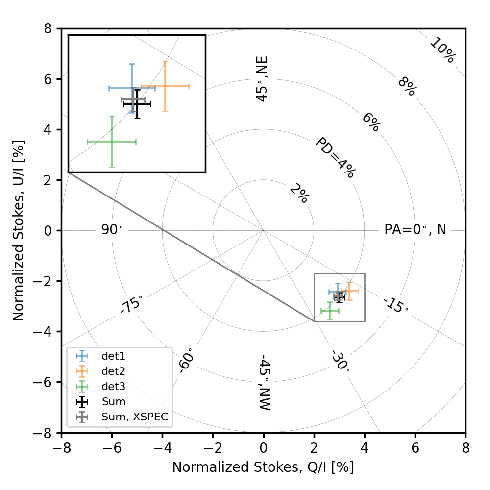
Figure S3: X-ray linear polarization of Cyg X-1 from the 2022 May 15 to 21 observations. The linear polarization of the x-rays from Cyg X-1 is shown in the plane of the normalized Stokes $Q/I$ and $U/I$ parameters measured with each of the three IXPE x-ray telescopes (coloured data points), and for the combined signal from all three telescopes (black). The grey data point shows the results from the analysis of the data using the xspec tool, instead of ixpeobssim . The two approaches give a result which is compatible within the statistical uncertainties. The circles give the contours of constant polarization degree (PD) while the radial lines correspond to constant polarization angle (PA). The error bars are 1 $\sigma$.

Figure S3 shows the IXPE polarization signal from the May 15 to May 21, 2022 observations in terms of the normalized Stokes parameters $Q/I$ and $U/I$, giving the polarized beam intensity along the north-south ($Q/I>0$) and east-west ($Q/I<0$) directions as well as along the northeast–southwest ($U/I>0$) and northwest–southeast ($U/I<0$) directions. Tables S1 and S2 give the results of both analyses in terms of the Stokes parameters, and polarization degree and angle, respectively. The consistency of the radio-jet – x-ray polarization alignment is limited by the precision of the radio results. Different studies have found $-26\hbox{${}^{\circ}$}$  (?), or $-21\hbox{${}^{\circ}$}$ to $-24\hbox{${}^{\circ}$}$ in 3 epochs, but $-17\hbox{${}^{\circ}$}$ for the inner jet in another epoch  (?). The variability of the results could be explained by the phase dependent absorption of the radio emission by the stellar wind  (?).

The target of opportunity observations of Cyg X-1 from June 18 to 20, 2022 showed the source still in the hard state. We measure a polarization degree and angle of 3.84$\pm$0.31% and $-25\mbox{$.\!\!^{\circ}$}7\pm 2\mbox{$.\!\!^{\circ}$}3$, respectively, for this data set. We present the results from the May and June observations as well as the results from the cumulative data set in Figure S4. The results are consistent with time independent polarization degree and polarization angle. The polarization degree and direction of the cumulative data set are 3.95$\pm$0.17% and $-22\mbox{$.\!\!^{\circ}$}2\pm 1\mbox{$.\!\!^{\circ}$}2$, respectively.

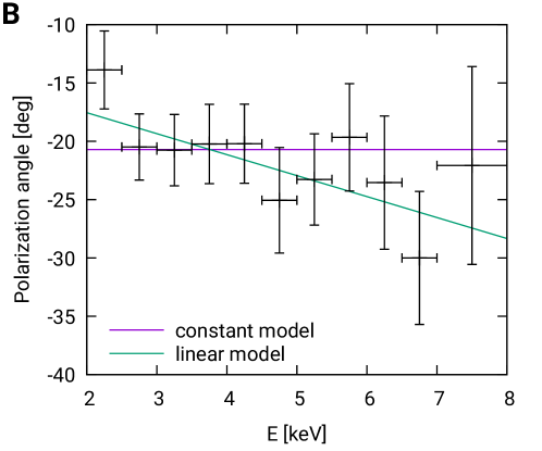
Figure S5: Energy dependence of the observed polarization degree (A) and polarization angle (B). The data (black crosses with 1$\sigma$ error bars) are produced using the PCUBE algorithm of the xpbin tool and summed over all detector units. The constant (violet) and linear (green) models fitted to the data are also depicted (see the text for details).

In the following we limit the analysis to the data acquired in May to avoid merging data taken a month apart. The polarization degree increases with energy from 3.5$\pm$0.2% in the energy band 2–5 keV to 5.3$\pm$0.5% in the energy band 5–8 keV  (?). Fitting a model of constant polarization is rejected at the 99.93% confidence level. The polarization degree (PD) increase with energy is better matched by a linear model $PD\,=\,A+B\times(E/{\rm keV}-1)$ with $A=(2.9\pm 0.4)\%$ and $B=(0.58\pm 0.15)\%$ (Figure S5 A). On theoretical grounds, we expect that the x-ray emission around the Fe K$\alpha$ line energy of 6.4 keV exhibits a reduced polarization degree. We find however, that the dips of the polarization degree at 4.5–5 and 6–6.5 keV are not statistically significant. The fit of a linear function has a $\chi^{2}$ of 4.04 for 9 degrees of freedom and a chance probability of larger $\chi^{2}$-values of 90.9%. Moreover, based on the constraints on the equivalent width of the fluorescent Fe K$\alpha$-line from the spectral analysis of the NICER and NuSTAR data, we find that the maximum possible Fe K$\alpha$ depolarization is much smaller than the observed dips. A fit of the polarization angle as a function of energy with a constant function gives a statistically acceptable fit with a chance probability for larger $\chi^{2}$-values of 57.5% (Figure S5 B).

The light curves in Figure S1 show that the Cyg X-1 IXPE count rates varied between 20 and 60 count s^-1. We investigated the flux dependence of the polarization properties by analyzing three count-rate selected data sets. The average fluxes of those data sets are 3.5, 3.9, and 4.5 times $10^{-9}$ erg cm^-2 s^-1. The polarization degree increase with the flux from $3.63\pm 0.30$% to $3.87\pm 0.34$% to $5.03\pm 0.41$% (Figure S6). The overall trend is statistically significant at the 98.3% confidence level.

Figure S7 shows that the polarization properties (Stokes $Q/I$ and $U/I$) do not depend on the orbital phase of the binary. Fitting the polarization along the orbit with a constant provides an acceptable null hypothesis probability. Data are summed between 2 and 8 keV. The assumed period is 5.599829 days, with $T_{0}$ at MJD 52872.288  (?).

IXPE, NICER, NuSTAR, and INTEGRAL energy spectra

We used the XSPEC package for fitting a simple model to the broadband Stokes $I$ spectrum provided by NICER, IXPE, NuSTAR, and INTEGRAL and the Stokes $Q$ and $U$ spectra provided only by IXPE. We use the data from the first NuSTAR observation and the simultaneously acquired NICER data, to eliminate differences due to spectral variability. We use the entire IXPE and INTEGRAL observations to maximize the signal-to-noise ratio. We fit the two NuSTAR Focal Plane Modules (FPMs) and the three IXPE detector inits separately in the fit. For the Stokes I spectrum, we employ the XSPEC fitting models

$$\textsc{mbpo}*\textsc{tbabs}*(\textsc{diskbb}+\textsc{xillverCp}+\textsc{relxillCp}+\textsc{nthComp}).$$ (S1)

Here diskbb represents thermal disk emission and nthComp represents Compton scattered emission observed directly from the corona. The relxillCp component represents coronal x-rays that are reflected from the inner accretion disk and distorted by relativistic effects. We assume that the flux irradiating the disk decreases with increasing radial distance proportional to $r^{-3}$. The xillverCp component represents coronal x-rays that are reflected from the outer disk and the companion star and not subject to strong relativistic effects. tbabs accounts for line-of-sight absorption by the interstellar medium.

The model mbpo is included to account for cross-calibration discrepancies we encountered between the four observatories. It multiplies the model spectrum by a broken power law, mbpo$(E)=N(E/E_{\rm br})^{\Delta\Gamma}$, where $E$ is the energy of the photon and $N$ is a normalization constant giving the ratio of the detection areas of the satellites at the energy $E_{\rm br}$ at which the power law index of the model changes from the value $\Delta\Gamma_{1}$ to $\Delta\Gamma_{2}$. For NICER, we fix the power-law indices to zero and the normalization to unity. For each NuSTAR FPM and INTEGRAL, we tie $\Delta\Gamma_{2}=\Delta\Gamma_{1}$ (i.e. employing only a single power law) but leave $\Delta\Gamma_{1}$ and $N$ as free parameters of the fit. For the IXPE detector units, we leave all mbpo parameters free. We also include a $0.5\%$ systematic uncertainty to further account for cross-calibration discrepancies. Finally, the NuSTAR FPM A disagrees with the FPM B and NICER in the 3–4 keV band, and IXPE detector unit #3 disagrees with all other instruments (even with the use of mbpo) in the $>5$ keV energy range, and so we ignore these ranges in our model fitting.

We first jointly fit the model to the NICER, NuSTAR and INTEGRAL data, then add IXPE Stokes $I$ to fit the model before finally adding IXPE Stokes $Q$ and $U$. At each stage, the best-fit parameters change by less than their uncertainties. We tie the seed photon temperature of the nthComp component (parameter $kT_{\rm bb}$) to the temperature of the inner edge of the accretion disk (parameter $k\,T_{\rm d}$ of the diskbb model). We tie the relxillCp photon index to that of the nthComp component, but are unable to do this for the seed photon temperature as this hardwired to $0.05$ keV in the relxillCp grid. We initially forced the relxillCp and nthComp components to have the same coronal electron temperature $k\,T_{\rm e}$, but found that the fit improved dramatically ($\gg 5~{}\sigma$ according to an F-test) after relaxing this assumption. The discrepancy between the corona temperature seen by the observer (nthComp temperature of 94 keV) and by the disc (relxillCp temperature of 140 keV) may be due to general relativistic effects (redshifting the emission seen by the observer), and due to the different viewing angles of the corona. We calculate $90\%$ confidence level uncertainties on the fitting results with a Markov Chain Monte Carlo simulation that uses the Goodman-Were algorithm with a total length of 307,200 steps spread over 256 walkers following an initial burn-in period of 19,968 steps. The best-fit spectral parameters are listed in Table Optical polarimetry.

Figure S8a shows the best-fit Stokes $I$ model and the data unfolded around that model, as well as the contributions from the different model components. The diskbb, xillverCp and relxillCp components contribute respectively 0.6%, 0.5% and 10.0% of the flux. The fractional contribution of each model component is consistent whether we consider only NICER, NuSTAR and INTEGRAL or also include IXPE. Because the direct coronal flux dominates the 2–8 keV flux, it must also dominate the polarization. For instance, the relativistic reflection component would need to be $\sim 40\%$ polarized to achieve the observed overall polarization of $\sim 4\%$. However, the reflected emission exhibits most likely much smaller polarization degree  (?, ?, ?, ?) (see also Figures S9 and S10).

As a simple toy model, we therefore assign a constant (independent of energy) polarization degree and angle to the nthComp component (the model polconst) and assume that the other components are unpolarized. Fig. S8c shows the resulting fit to IXPE Stokes Q and U. We find a reduced $\chi^{2}$ of $\chi^{2}/({\rm degrees\,of\,freedom)}=2575.72/2466$. Panel Fig S8d shows the contributions from each energy channel to $\chi$, we find that there are no structured residuals. The best-fit polarization degree and angle of the corona from this simple model are respectively $3.63\pm 0.26\%$ and $-20\mbox{$.\!\!^{\circ}$}5\pm 2\mbox{$.\!\!^{\circ}$}1$ ($90\%$ confidence).

Model constraints on the inclination of the inner accretion disk

We studied the energy spectra and polarization properties of different corona shapes and properties with the raytracing codes kerrC  (?), Monk  (?), and with an iterative radiation transport solver  (?, ?). We present simulation results that match the IXPE, NICER, and NuSTAR energy spectra qualitatively, and the predicted polarization properties.

The Cyg X-1 binary system spins clockwise  (?); we therefore plot position angles assuming that the inner disk and the black hole also spin clockwise. This assumption impacts the sign of the predicted polarization angles. We assume furthermore that the inner disk and black hole spin axes are aligned and are at 0^∘ position angle. The position angles shown in Figure 3 were obtained by subtracting $22\hbox{${}^{\circ}$}$ from the position angles in the models.

We used the general relativistic ray tracing codes kerrC to evaluate the polarization that cone-shaped coronae centered on the black hole spin axes and wedge-shaped coronae sandwiching the accretion disk can produce. The code assumes a standard geometrically thin, optically thick accretion disk extending from the innermost stable circular orbit to 100 gravitational radii $r_{\rm g}=G\,M/c^{2}$ with $G$ being the gravitational constant, $M$ the black hole mass, and $c$ the speed of light. The code uses Monte Carlo methods to simulate the polarized emission of the accretion disk photons assuming Novikov-Thorne temperature profiles, the geodesic propagation of the x-rays including the general relativistic polarization direction evolution, the polarization-changing Compton scattering of the photons in the corona, and the reflection of the photons off the accretion disk adopting the XILLVER reflection model for the reflected intensity  (?, ?, ?), and an analytical solution for the reflected polarization  (?). In both cases, we chose corona parameters which maximize the predicted polarization degree, i.e., cone-shaped coronae close to the accretion disk, and thin wedge-shaped coronae with a half opening angle of 10^∘. The model parameters are given in Table S3. For all models, we assume that the black hole spin vector and the inner disk spin vector are aligned. The sandwich and cone corona models (as well as the extended lamppost corona model discussed below) are phenomenological - the coronal temperatures are not derived self-consistently. Coronae could cool radiatively, to the point that the predicted energy spectra are softer than the observed ones  (?, ?). Processes that heat and cool the coronal plasma are debated, as are their relative contributions  (?, ?, ?).

We also used the ray tracing code Monk, which is similar to kerrC but implements the simulation of an extended lamppost corona. The lamppost corona is centered on the spin axis of the accretion disk at a radial coordinate of $r\,=\,$10$\,r_{\rm g}$ and has a radius of 8 $r_{\rm g}$, an electron temperature of 100 keV, and Thomson optical depth of 1 (defined as $n_{e}\sigma_{\rm T}R_{c}$, where $n_{e}$ is the electron density of the corona, $\sigma_{\rm T}$ is the Thomson cross section, and $R_{c}$ is the radius of the corona). Simulations were performed for both Schwarzschild ($a=0$) and Kerr ($a=0.998$) black holes, with mass accretion rate of $4.71\times 10^{17}$ and $2.64\times 10^{18}~{}\rm g~{}s^{-1}$, respectively. For the Monk simulations, we first calculated the Stokes parameters generated by the direct emission and then added those of the reflected emission. The reflected emission was normalized to reproduce the reflected emission fraction from the analysis of the NICER, IXPE, NuSTAR, and INTEGRAL energy spectra. We compared the Monk results before and after accounting for the reflected emission. The reflected emission lowers the total polarization degree by $\sim$20% (e.g.  a polarization degree of 3% before accounting for reflection becomes 2.5% after accounting for the impact of reflection) as the different polarization directions of the direct and reflected emission components lead to the partial cancellation of the different polarizations.

We studied the polarization of the truncated disk/inner hot flow scenario with the iterative radiation transport solver mentioned above. The code treats Compton scattering of polarized radiation in a plane-parallel geometry in flat space. It uses exact Compton scattering redistribution matrices for isotropic electrons  (?) and solves the polarized radiation transfer equations using an expansion of the intensities in scattering orders. We do not include reflection off the cold disk  (?) to avoid uncertainties related to the properties of the reflecting plasma. The code simulates a plane parallel slab, using a prescription to inject seed photons that mimics the truncated disk scenario with the hot flow height-to-radius ratio of 1. The electron temperature is assumed to be $kT_{\rm e}=100$ keV, the seed blackbody temperature $kT_{\rm bb}=0.1$ keV and the Thomson optical depth $\tau_{\rm T}=1.0$  (?, ?). Analytical prescriptions are used to account for the impact of special and general relativistic effects on the observed polarization degree and angle  (?) in the Schwarzschild metrics.

Figures S9 and S10 summarize the polarization predictions. Figure S9 shows the simulation results for models with coronae extending parallel to the accretion disk. The sandwich corona simulated with kerrC generates sufficiently large polarization degree for $i\gtrsim 60\hbox{${}^{\circ}$}$. The polarization direction aligns within a few degrees with the inner disk spin axis. The hot inner flow inside a truncated disk exhibits higher polarization degree at lower energies than the sandwich corona. We interpret this difference as follows: for the sandwich corona, the first scatterings of photons coming from the accretion disk and scattering towards the observer create a net polarization parallel to the accretion disk that competes with the perpendicular polarization of the emission scattering multiple times in the plane of the corona. In contrast, the first scatterings of truncated disk photons entering the hot inner flow from the sides create a net perpendicular polarization similar to the perpendicular polarization of the photons scattering multiple times in the plane of the hot flow. In principle, high-precision polarization measurements can distinguish between the two models. However, the uncertainties about the shape and properties of the corona and the disk preclude us from drawing firm conclusions.

The polarization degree of the observed keV photons are higher if the corona Compton scatters synchrotron photons (rather than accretion disk photons). In this case, $\sim$4% polarization degrees can already be observed for $i\geq 45^{\circ}$ (Figure S9). As the synchrotron photons initially have lower energies ($\sim$1–10 eV) than the accretion disk photons ($\sim$0.1 keV), more scatterings are required to scatter them into the keV energy range, leading to high but rather constant 2-8 keV polarization degrees.

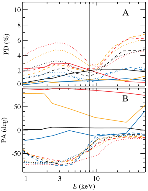
Figure S10: Same as Figure S9, but for models with coronae located on the spin axis of the accretion disk. The solid lines show the predictions for a cone-shaped corona extended along the disk spin axis, the dashed and dotted lines shows the results for an extended lamppost corona for a non-spinning black hole ($a=0$, dashed line) and a spinning black hole ($a=0.998$, dotted line).

Figure S10 shows the simulation results for models with coronae located on the spin axis of the accretion disk. The cone shaped corona simulated with kerrC includes the effects of the reflected emission and exhibits small ($<2\%$) 2–8 keV polarization degree for $i=30\hbox{${}^{\circ}$}$ and $i=45\hbox{${}^{\circ}$}$ inclinations. For $i=60\hbox{${}^{\circ}$}$, the polarization of the emission from the corona reaching the observer directly, and the emission from the corona reflecting off the disk cancel to give $\lesssim 1\%$ polarization degree at all energies. For $i=75\hbox{${}^{\circ}$}$, the polarization parallel to the disk is higher, giving a net polarization was calculated reaching $\sim$3%. Although even larger inclination can produce polarization degree meeting or exceeding the observed 4% polarization degree, the direction stays parallel to the disk, contradicting the observed alignment of the polarization direction and the radio jet. The polarization of the Monk extended lamppost model (including the effect of the reflected emission) was calculated for $a=0$ and $a=0.998$, respectively. The high-spin models exhibit polarization degree meeting or exceeding the observed 4% polarization degree but again, the polarization direction is parallel to the accretion disk.

Optical polarimetry

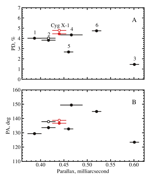
Figure S12: Polarization of nearby field stars around Cyg X-1 as a function of parallax. (A) Polarization degree (PD) and (B) polarization angle (PA) for a set of field stars (black) and Cyg X-1 (red) as measured with DIPol-2 (filled circles) and RoboPol (open circles) in the $R$-band. Error bars show uncertainties at the 1$\sigma$ confidence level.

The optical polarimetric observations were performed using DIPol-2 polarimeter, installed on the remotely operated Tohoku 60 cm (T60) telescope at the Haleakala Observatory, Hawaii. DIPol-2 is a double-image CCD polarimeter, capable of measuring linear and circular polarization in three ($B$, $V$, and $R$) optical filters simultaneously  (?, ?). The design of this instrument optically eliminates the sky polarization (even if it is variable) to a polarization level of $<10^{-5}$. The instrumental polarization is $<10^{-4}$ and measured by observing twenty unpolarized nearby stars. The zero point of the polarization angle was determined by observing two highly polarized standard stars (HD 20 4827 and HD 25 443). We observed Cyg X-1 for five nights during the week 2022 May 15 to 21, for about 4 hours each night. Each measurement of Stokes parameters took about 20 s and we obtained 2298 simultaneous measurements of the normalized Stokes parameters $q_{\rm obs}=Q_{\rm obs}/I_{\rm obs}$ and $u_{\rm obs}=U_{\rm obs}/I_{\rm obs}$ in the three filters ($B$, $V$, and $R$). These individual measurements were used to compute average intranight values of Stokes parameters using the $2\sigma$ weighting algorithm  (?, ?). The uncertainty of the final average corresponds to the standard deviation of individual measurements resulting from the orbital variability of the source. The polarization produced by the interstellar (IS) medium was estimated by observing a sample of field stars (Figure S11), which are close in distance to the target as indicated by their Gaia parallaxes (Figure S12)  (?, ?). Taking into account angular separation on the image, closeness in distance, and the wavelength dependence of the polarization, we choose two stars (designating them Ref 1 and Ref 2) from our sample as the IS polarization standards (see Figure S11). We considered two cases: the Stokes parameters of the IS polarization were set to be equal to those of Ref 2, and, alternatively, to the weighted average of those of Ref 1 and Ref 2. For both cases, the normalized Stokes parameters ($q_{\rm is}$, $u_{\rm is}$) were subtracted from the measured values of Stokes parameters of the target ($q_{\rm obs}$, $u_{\rm obs}$) to obtain the intrinsic polarization ($q_{\rm int}$, $u_{\rm int}$) estimates. From this we determine the intrinsic polarization degree (PD) and polarization angle (PA) as

$$\mbox{PD}=\sqrt{q_{\rm int}^{2}+u_{\rm int}^{2}},\quad\mbox{PA}=\frac{1}{2}{\rm atan}2(u_{\rm int},q_{\rm int}).$$ (S2)

The uncertainty on the polarization degree $\Delta\mbox{(PD)}$ was estimated as the uncertainty of the individual Stokes parameters, and includes both the source and IS polarization uncertainties. The uncertainty on the polarization angle (in radians) was estimated as $\Delta\mbox{(PA)}=\Delta\mbox{(PD)}/(2\,\mbox{PD})$  (?). The observed normalized Stokes parameters, the IS polarization and the intrinsic Stokes parameters as well as the polarization degree and polarization angle are reported in Table S4.

We used the RoboPol polarimeter in the focal plane of the 1.3 m telescope of the Skinakas observatory (Greece) to obtain additional $R$-band polarimetry. The observations were performed between 2022 May 13 and June 2 with multiple pointings in 10 nights. In total, 21 exposures series were acquired, each series consisting of 10 to 20 exposures, each of 1 to 2 seconds duration. The instrumental polarization was found with a set of unpolarized standards stars (BD +28 4211, BD +33 2642, BD +32 3739, BD +40 2704, HD 154 892). The zero polarization angle was determined based on three highly polarized standard stars (VI Cyg 12, Hiltner 960 and CygOB2 14). The Cyg X-1 measurements do not reveal any polarization variability exceeding that of the standard stars (for which the standard deviation from the mean values, $\sigma_{q}=0.12\%,\sigma_{u}=0.08\%$, were obtained). We determined the average polarization parameters of Cyg X-1 from calculating the sigma-clipped median of the relative Stokes parameters. The uncertainties were determined by error propagation adding the instrumental polarization uncertainties in quadrature. We determined the intrinsic source polarization by subtracting the IS polarization using the same Ref 2 star as used in the DIPol-2 analysis (Table S4).

We find optical polarization angles of Cyg X-1 between $-37\hbox{${}^{\circ}$}$ to $-11\hbox{${}^{\circ}$}$, close to the position angle of the jet from radio interferometry (from $-26\hbox{${}^{\circ}$}$ to $-9\hbox{${}^{\circ}$}$)  (?, ?). The blue supergiant companion star dominates the optical emission from Cyg X-1  (?). The optical polarization is likely produced by the scattering of the stellar radiation off the bulge formed by the accretion stream interacting with the accretion disk  (?).

Figure S9: Polarization degree (A) and polarization angle (B) for models with coronae extending parallel to the accretion disk. The solid lines show the predictions of the sandwich corona, the dashed and dotted lines show the predictions of the hot inner flow inside a truncated disk, with accretion disk photons (dashed lines) and synchrotron photons (dotted lines) acting as seed photons for the inverse Compton scattering. The colors encode the inclination angle at which the coronae are observed: red (75^∘), orange (60^∘), black (45^∘) and blue (30^∘). The vertical lines delineate the IXPE band from 2–8 keV. For very low polarization degrees the polarization angle in the sandwich corona model fluctuates by a few degrees owing to the finite number of simulated events. Positive polarization angles correspond to counterclockwise rotations of the polarization vector relative to the projected disk spin axis on the plane of the sky in Figure 3.

Table S1: IXPE polarization results given in terms of the Stokes parameters. Values are derived for the data collected independently by each individual IXPE telescopes and for their sum with the ixpeobssim and (only for the sum) with xspec analysis. The two methods and the independent analysis of single IXPE telescopes provide consistent results. The uncertainties are 68.3% confidence interval, assuming that the Stokes parameters are independent.

	2.0–3.0 keV	3.0–4.0 keV	4.0–6.0 keV	6.0–8.0 keV	2.0–8.0 keV
$Q/I$ - det1 [%]	$2.9\pm 0.5$	$2.5\pm 0.5$	$3.4\pm 0.6$	$3.0\pm 1.4$	$2.9\pm 0.3$
$Q/I$ - det2 [%]	$3.3\pm 0.5$	$2.5\pm 0.5$	$3.9\pm 0.6$	$4.7\pm 1.4$	$3.4\pm 0.3$
$Q/I$ - det3 [%]	$2.1\pm 0.5$	$2.7\pm 0.5$	$3.1\pm 0.6$	$3.4\pm 1.6$	$2.6\pm 0.4$
$Q/I$ - sum [%]	$2.8\pm 0.3$	$2.5\pm 0.3$	$3.5\pm 0.3$	$3.7\pm 0.8$	$3.0\pm 0.2$
$Q/I$ - sum (xspec) [%]	$2.9\pm 0.3$	$2.7\pm 0.3$	$3.4\pm 0.3$	$3.7\pm 0.8$	$2.9\pm 0.2$
$U/I$ - det1 [%]	$-2.1\pm 0.5$	$-1.9\pm 0.5$	$-2.8\pm 0.6$	$-4.2\pm 1.4$	$-2.4\pm 0.3$
$U/I$ - det2 [%]	$-1.3\pm 0.5$	$-2.3\pm 0.5$	$-2.7\pm 0.6$	$-6.0\pm 1.4$	$-2.4\pm 0.3$
$U/I$ - det3 [%]	$-2.9\pm 0.5$	$-2.9\pm 0.5$	$-4.0\pm 0.6$	$-2.9\pm 1.6$	$-3.2\pm 0.4$
$U/I$ - sum [%]	$-2.1\pm 0.3$	$-2.3\pm 0.3$	$-3.1\pm 0.3$	$-4.5\pm 0.8$	$-2.7\pm 0.2$
$U/I$ - sum (xspec) [%]	$-2.3\pm 0.3$	$-2.4\pm 0.3$	$-3.2\pm 0.3$	$-4.2\pm 0.8$	$-2.6\pm 0.3$

Table S2: IXPE polarization results given in terms of the polarization degree and angle. Uncertainties are given on 68.3% confidence level, and were calculated from the Stokes parameters reported in Table S1 assuming that the polarization degree and polarization angle are independent. The significance was calculated as the measured polarization degree divided by the uncertainty, for the sum of the three IXPE telescopes.

	2.0–3.0 keV	3.0–4.0 keV	4.0–6.0 keV	6.0–8.0 keV	2.0–8.0 keV
PD - det1 [%]	$3.5\pm 0.5$	$3.1\pm 0.5$	$4.4\pm 0.6$	$5.1\pm 1.4$	$3.8\pm 0.3$
PD - det2 [%]	$3.6\pm 0.5$	$3.4\pm 0.5$	$4.7\pm 0.6$	$7.6\pm 1.4$	$4.2\pm 0.3$
PD - det3 [%]	$3.6\pm 0.5$	$3.9\pm 0.5$	$5.1\pm 0.6$	$4.5\pm 1.6$	$4.1\pm 0.4$
PD - sum [%]	$3.5\pm 0.3$	$3.5\pm 0.3$	$4.7\pm 0.3$	$5.8\pm 0.8$	$4.0\pm 0.2$
PD - sum (xspec) [%]	$3.7\pm 0.3$	$3.6\pm 0.3$	$4.7\pm 0.3$	$5.6\pm 0.8$	$3.9\pm 0.2$
PD significance	13$\sigma$	12$\sigma$	14$\sigma$	7$\sigma$	20$\sigma$
PA - det1 [deg]	$-18\pm 4$	$-19\pm 4$	$-20\pm 4$	$-27\pm 8$	$-20\pm 3$
PA - det2 [deg]	$-11\pm 4$	$-22\pm 4$	$-17\pm 4$	$-26\pm 5$	$-18\pm 2$
PA - det3 [deg]	$-27\pm 4$	$-23\pm 4$	$-26\pm 4$	$-20\pm 10$	$-25\pm 2$
PA - sum [deg]	$-18\pm 2$	$-21\pm 2$	$-21\pm 2$	$-25\pm 4$	$-21\pm 1$
PA - sum (xspec) [deg]	$-19\pm 2$	$-21\pm 2$	$-21\pm 2$	$-25\pm 4$	$-21\pm 1$

Table S3: Parameters of the kerrC models shown in Figures S9 and S10.

Parameter	Symbol	Unit	wedge	cone
Black hole spin	$a$	none	0.9	0.9
Black hole mass	$M$	solar masses	21.2	21.2
Corona temperature	$T_{\rm C}$	keV	100	150
Optical depth	$\tau_{\rm C}$	none	0.35	0.79
Opening angle	$\theta_{\rm C}$	deg	10	25
Corona inner/outer edge	$r_{1},r_{2}$	$r_{\rm g}$	2.32/100	2.5/20
Inclination	$i$	deg	65	85
Accretion rate	$\dot{M}$	1018 g s-1	0.0505	0.1
Cyg X-1 distance	$d$	kpc	2.22	2.22
Axis position angle	$\psi$	deg	0	0
XILLVER metal abundance relative to solar	$A_{\rm Fe}$	none	1	1
XILLVER electron temperature	$T_{\rm e}$	keV	100	150
XILLVER $e^{-}$-density in cm-3	$\log_{10}(n_{\rm e})$	none	17.5	17.7
Equivalent hydrogen column density	$N_{\rm H}$	$10^{22}$ cm-2	0.2	4

Table S4: Optical polarization of Cyg X-1. Normalized Stokes parameters $q$ and $u$ are presented for the observed polarization of the source ($q_{\rm obs}$, $u_{\rm obs}$), the IS polarization ($q_{\rm is}$, $u_{\rm is}$), and the intrinsic polarization obtained by subtracting the IS polarization from the observed values ($q_{\rm int}$, $u_{\rm int}$). The polarization degree (PD) and polarization angle (PA) of the intrinsic polarization are computed using formulae (S2). Uncertainties are 1$\sigma$.

Band	$B$		$V$		$R$
	$q$ (%)	$u$ (%)	$q$ (%)	$u$ (%)	$q$ (%)	$u$ (%)
Observed polarization of Cyg X-1
DIPol-2	$\phantom{-}0.46\pm 0.06$	$-4.89\pm 0.04$	$\phantom{-}0.39\pm 0.04$	$-4.57\pm 0.04$	$\phantom{-}0.26\pm 0.03$	$-4.44\pm 0.03$
RoboPol	–	–	–	–	$\phantom{-}0.61\pm 0.13$	$-4.74\pm 0.12$
Interstellar polarization
Ref 2/DIPol-2	$-0.09\pm 0.17$	$-4.31\pm 0.17$	$-0.12\pm 0.14$	$-3.91\pm 0.14$	$-0.19\pm 0.15$	$-3.82\pm 0.15$
Ref 1+2/DIPol-2	$-0.41\pm 0.11$	$-4.39\pm 0.11$	$-0.33\pm 0.10$	$-3.92\pm 0.10$	$-0.67\pm 0.07$	$-4.05\pm 0.07$
Ref 2/RoboPol	–	–	–	–	$\phantom{-}0.39\pm 0.16$	$-4.00\pm 0.08$
Intrinsic polarization of Cyg X-1-
Ref 2/DIPol-2	$\phantom{-}0.55\pm 0.17$	$-0.58\pm 0.17$	$\phantom{-}0.51\pm 0.14$	$-0.66\pm 0.14$	$\phantom{-}0.45\pm 0.15$	$-0.62\pm 0.15$
Ref 1+2/DIPol-2	$\phantom{-}0.87\pm 0.11$	$-0.50\pm 0.11$	$\phantom{-}0.72\pm 0.10$	$-0.65\pm 0.10$	$\phantom{-}0.93\pm 0.07$	$-0.39\pm 0.07$
Ref 2/RoboPol	–	–	–	–	$\phantom{-}0.22\pm 0.21$	$-0.74\pm 0.14$
Intrinsic polarization of Cyg X-1
	PD (%)	PA (deg)	PD (%)	PA (deg)	PD (%)	PA (deg)
Ref 2/DIPol-2	$\phantom{-}0.79\pm 0.17$	$-23\pm 6$	$\phantom{-}0.83\pm 0.14$	$-26\pm 5$	$\phantom{-}0.77\pm 0.15$	$-27\pm 6$
Ref 1+2/DIPol-2	$\phantom{-}1.00\pm 0.11$	$-15\pm 3$	$\phantom{-}0.97\pm 0.10$	$-21\pm 3$	$\phantom{-}1.01\pm 0.07$	$-11\pm 2$
Ref 2/RoboPol	–	–	–	–	$\phantom{-}0.77\pm 0.15$	$-37\pm 6$

Table S5: Best-fit parameters of the spectro-polarimetric model fitted to the data (Equation S1) Other xillverCp parameters were tied to the corresponding relxillCp parameters. The relxillCp reflection fraction has been multiplied by 15.043 to account for nthComp and relxillCp being normalized differently. The uncertainties are given on the 90% confidence level.

Component	Parameter (unit)	Description	Value
TBabs	$N_{\rm H}$ ($10^{22}$ cm-2)	Hydrogen column density	$0.437^{+0.025}_{-0.10}$
diskbb	$kT_{\rm d}$ (keV)	Peak disk temperature	$0.319^{+0.018}_{-0.018}$
	norm ($10^{3}$)	Normalization	$3.79^{+0.90}_{-1.3}$
nthComp	$\Gamma$	Photon index	$1.62^{+0.0043}_{-0.0078}$
	$kT_{\rm e}$ (keV)	Electron temperature	$94.2^{+2.4}_{-6.8}$
	norm	Normalization	$0.945^{+0.050}_{-0.044}$
	PD (%)	polarization degree	$3.63^{+0.26}_{-0.26}$
	PA (deg)	polarization angle	$-20.5^{+2.1}_{-2.1}$
relxillCp	$r_{\rm in}$ ($r_{g}$)	Disk inner radius	$3.35^{+0.62}_{-0.41}$
	$i$ (deg)	Disk inclination angle	$37.8^{+1.2}_{-2.9}$
	$\log_{10}(\xi/[{\rm erg}~{}{\rm cm}~{}{\rm s}^{-1}])$	Ionization parameter	$3.15^{+0.040}_{-0.031}$
	$kT_{\rm e}$ (keV)	Electron temperature	$140^{+32}_{-42}$
	$A_{\rm Fe}$ (solar)	Iron abundance	$3.70^{+0.50}_{-0.21}$
	$f$ (%)	Reflection fraction	$20.17^{+1.6}_{-2.8}$
xillverCp	$\log_{10}(\xi/[{\rm erg}~{}{\rm cm}~{}{\rm s}^{-1}])$	Ionization parameter	$2.25^{+0.099}_{-0.19}$
	norm ($10^{-3}$)	Normalization	$3.46^{+0.14}_{-0.72}$
mbpo NuSTAR FPMA	$\Delta\Gamma_{1}$ ($10^{-2}$)	Power-law index	$-6.22^{+0.60}_{-0.67}$
	$N$	Normalization	$1.13^{+0.0081}_{-0.0038}$
mbpo NuSTAR FPMB	$\Delta\Gamma_{1}$ ($10^{-2}$)	Power-law index	$-7.11^{+0.56}_{-0.61}$
	$N$	Normalization	$1.17^{+0.0051}_{-0.0034}$
mbpo INTEGRAL	$\Delta\Gamma_{1}$ ($10^{-2}$)	Power-law index	$-13.8^{+2.2}_{-1.7}$
	$N$	Normalization	$1.44^{+0.018}_{-0.075}$
mbpo IXPE DU1	$\Delta\Gamma_{1}$ ($10^{-2}$)	Low energy power-law index	$1.34^{+1.8}_{-1.8}$
	$\Delta\Gamma_{2}$ ($10^{-2}$)	High energy power-law index	$-22.2^{+1.3}_{-1.3}$
	$E_{\rm br}$ (keV)	Break energy	$3.28^{+0.13}_{-0.10}$
	$N$	Normalization	$1.51^{+0.0071}_{-0.0084}$
mbpo IXPE DU2	$\Delta\Gamma_{1}$ ($10^{-2}$)	Low energy power-law index	$-5.61^{+1.7}_{-1.4}$
	$\Delta\Gamma_{2}$ ($10^{-2}$)	High energy power-law index	$-27.9^{+1.6}_{-2.2}$
	$E_{\rm br}$ (keV)	Break energy	$3.54^{+0.19}_{-0.15}$
	$N$	Normalization	$1.45^{+0.0011}_{-0.013}$
mbpo IXPE DU3	$\Delta\Gamma_{1}$ ($10^{-2}$)	Low energy power-law index	$-8.82^{+1.6}_{-1.7}$
	$\Delta\Gamma_{2}$ ($10^{-2}$)	High energy power-law index	$-29.5^{+3.1}_{-3.3}$
	$E_{\rm br}$ (keV)	Break energy	$3.33^{+0.18}_{-0.15}$
	$N$	Normalization	$1.44^{+0.012}_{-0.014}$

References

- 1. J. C. A. Miller-Jones, et al., Science 371, 1046 (2021).
- 2. L. Gou, et al., Astrophys. J. 790, 29 (2014).
- 3. A. M. Stirling, et al., Mon. Not. R. Astron. Soc. 327, 1273 (2001).
- 4. C. Done, M. Gierliński, A. Kubota, Astron. Astrophys. Rev. 15, 1 (2007).
- 5. P. A. Connors, T. Piran, R. F. Stark, Astrophys. J. 235, 224 (1980).
- 6. L.-X. Li, R. Narayan, J. E. McClintock, Astrophys. J. 691, 847 (2009).
- 7. J. D. Schnittman, J. H. Krolik, Astrophys. J. 701, 1175 (2009).
- 8. C. Bambi, et al., Space Sci. Rev. 217, 65 (2021).
- 9. J. D. Schnittman, J. H. Krolik, Astrophys. J. 712, 908 (2010).
- 10. G. Matt, Mon. Not. R. Astron. Soc. 260, 663 (1993).
- 11. J. Poutanen, K. N. Nagendra, R. Svensson, Mon. Not. R. Astron. Soc. 283, 892 (1996).
- 12. M. C. Weisskopf, et al., J. Astron. Telesc. Instrum. Syst. 8, 026002 (2022).
- 13. H. Krawczynski, B. Beheshtipour, Astrophys. J. 934, 4 (2022).
- 14. M. C. Weisskopf, et al., Astrophys. J. Lett. 215, L65 (1977).
- 15. K. S. Long, G. A. Chanan, R. Novick, Astrophys. J. 238, 710 (1980).
- 16. M. Chauvin, et al., Nature Astronomy 2, 652 (2018).
- 17. Materials and methods are available as supplementary materials.
- 18. J. C. Kemp, M. S. Barbour, T. E. Parker, L. C. Herman, Astrophys. J. Lett. 228, L23 (1979).
- 19. M. C. Begelman, R. D. Blandford, M. J. Rees, Reviews of Modern Physics 56, 255 (1984).
- 20. F. Haardt, L. Maraschi, Astrophys. J. Lett. 380, L51 (1991).
- 21. B. E. Kinch, J. D. Schnittman, S. C. Noble, T. R. Kallman, J. H. Krolik, Astrophys. J. 922, 270 (2021).
- 22. F. Meyer, E. Meyer-Hofmeister, Astron. & Astrophys. 288, 175 (1994).
- 23. P. O. Petrucci, J. Ferreira, G. Henri, J. Malzac, C. Foellmi, Astron. & Astrophys. 522, A38 (2010).
- 24. A. Veledina, J. Poutanen, I. Vurm, Mon. Not. R. Astron. Soc. 430, 3196 (2013).
- 25. J. M. Bardeen, J. A. Petterson, Astrophys. J. Lett. 195, L65 (1975).
- 26. J. A. Tomsick, et al., Astrophys. J. 780, 78 (2014).
- 27. M. L. Parker, et al., Astrophys. J. 808, 9 (2015).
- 28. P. Lachowicz, A. A. Zdziarski, A. Schwarzenberg-Czerny, G. G. Pooley, S. Kitamoto, Mon. Not. R. Astron. Soc. 368, 1025 (2006).
- 29. D. M. Russell, T. Shahbaz, Mon. Not. R. Astron. Soc. 438, 2083 (2014).
- 30. A. A. Zdziarski, P. Pjanka, M. Sikora, Ł. Stawarz, Mon. Not. R. Astron. Soc. 442, 3243 (2014).
- 31. M. Lyutikov, V. I. Pariev, D. C. Gabuzda, Mon. Not. R. Astron. Soc. 360, 869 (2005).
- 32. P. Thalhammer, J. Wilms, N. Rodriguez Cavero, Zenodo, DOI: 10.5281/zenodo.7140274 (2022).
- 33. V. Kravtsov, et al., Zenodo, DOI: 10.5281/zenodo.7108247 (2022).
- 34. D. Blinov, S. Kiehlmann, N. Mandarakas, R. Skalidis, Zenodo, DOI: 10.5281/zenodo.7127802 (2022).
- 35. W. Zhang, M. Dovčiak, M. Bursa, Astrophys. J. 875, 148 (2019).
- 36. A. Veledina, J. Poutanen, Zenodo, DOI: 10.5281/zenodo.7116125 (2022).
- 37. K. A. Arnaud, “XSPEC: The First Ten Years”, Astronomical Data Analysis Software and Systems V, G. H. Jacoby, J. Barnes, eds. (1996), vol. 101 of Astronomical Society of the Pacific Conference Series, pp. 17–20.
- 38. P. Freeman, S. Doe, A. Siemiginowska, “Sherpa: a mission-independent data analysis application”, Astronomical Data Analysis, J.-L. Starck, F. D. Murtagh, eds. (2001), vol. 4477 of Society of Photo-Optical Instrumentation Engineers (SPIE) Conference Series, pp. 76–87.
- 39. S. Doe, et al., “Developing Sherpa with Python”, Astronomical Data Analysis Software and Systems XVI, R. A. Shaw, F. Hill, D. J. Bell, eds. (2007), vol. 376 of Astronomical Society of the Pacific Conference Series, p. 543.
- 40. B. L. Refsdal, et al., “Sherpa: 1D/2D modeling and fitting in Python”, Proceedings of the 8th Python in Science Conference, G. Varoquaux, S. van der Walt, J. Millman, eds. (Pasadena, CA USA, 2009), pp. 51 – 57.
- 41. B. Refsdal, S. Doe, D. Nguyen, A. Siemiginowska, “Fitting and Estimating Parameter Confidence Limits with Sherpa”, Proceedings of the 10th Python in Science Conference, S. van der Walt, J. Millman, eds. (2011), pp. 10 – 16.
- 42. F. Kislat, B. Clark, M. Beilicke, H. Krawczynski, Astroparticle Physics 68, 45 (2015).
- 43. L. Baldini, et al., SoftwareX 19, 101194 (2022), https://ixpeobssim.readthedocs.io/en/latest/?badge=latest, https://github.com/lucabaldini/ixpeobssim. Accessed: 2012-10-05.
- 44. M. C. Weisskopf, R. F. Elsner, S. L. O’Dell, “On understanding the figures of merit for detection and measurement of x-ray polarization”, Space Telescopes and Instrumentation 2010: Ultraviolet to Gamma Ray, M. Arnaud, S. S. Murray, T. Takahashi, eds. (2010), vol. 7732 of Society of Photo-Optical Instrumentation Engineers (SPIE) Conference Series, p. 77320E.
- 45. F. Muleri, “Analysis of the data from photoelectric gas polarimeters”, Handbook of X-ray and Gamma-ray Astrophysics, C. Bambi, A. Santangelo, eds. (Springer, Singapore, in press).
- 46. T. E. Strohmayer, Astrophys. J. 838, 72 (2017).
- 47. F. A. Harrison, et al., Astrophys. J. 770, 103 (2013).
- 48. Heasoft, “a unified release of the ftools and xanadu software packages”, https://heasarc.gsfc.nasa.gov/docs/software/heasoft/. Accessed: 2012-09-22.
- 49. K. C. Gendreau, Z. Arzoumanian, T. Okajima, “The Neutron star Interior Composition ExploreR (NICER): an Explorer mission of opportunity for soft x-ray timing spectroscopy”, Space Telescopes and Instrumentation 2012: Ultraviolet to Gamma Ray, T. Takahashi, S. S. Murray, J.-W. A. den Herder, eds. (2012), vol. 8443 of Society of Photo-Optical Instrumentation Engineers (SPIE) Conference Series, p. 844313.
- 50. M. Pavlinsky, et al., Astron. & Astrophys. 650, A42 (2021).
- 51. R. Sunyaev, et al., Astron. & Astrophys. 656, A132 (2021).
- 52. Integral off-line scientific analysis software (osa), https://heasarc.gsfc.nasa.gov/docs/integral/inthp_analysis.html. Accessed: 2012-09-22.
- 53. M. Matsuoka, et al., Publ. Astron. Soc. Japan 61, 999 (2009).
- 54. R. Whitehurst, A. King, Mon. Not. R. Astron. Soc. 249, 25 (1991).
- 55. M. M. Kotze, P. A. Charles, Mon. Not. R. Astron. Soc. 420, 1575 (2012).
- 56. J. Poutanen, A. A. Zdziarski, A. Ibragimov, Mon. Not. R. Astron. Soc. 389, 1427 (2008).
- 57. D. R. Gies, et al., Astrophys. J. 678, 1237 (2008).
- 58. M. Dovčiak, F. Muleri, R. W. Goosmann, V. Karas, G. Matt, Astrophys. J. 731, 75 (2011).
- 59. J. Podgorný, M. Dovčiak, F. Marin, R. Goosmann, A. Różańska, Mon. Not. R. Astron. Soc. 510, 4723 (2022).
- 60. J. Poutanen, R. Svensson, Astrophys. J. 470, 249 (1996).
- 61. J. García, T. R. Kallman, R. F. Mushotzky, Astrophys. J. 731, 131 (2011).
- 62. J. García, et al., Astrophys. J. 768, 146 (2013).
- 63. J. García, et al., Astrophys. J. 782, 76 (2014).
- 64. S. Chandrasekhar, Radiative transfer (Dover Publications, 1960).
- 65. J. Malzac, A. M. Dumont, M. Mouchet, Astron. & Astrophys. 430, 761 (2005).
- 66. J. Poutanen, A. Veledina, A. A. Zdziarski, Astron. & Astrophys. 614, A79 (2018).
- 67. K. Nishikawa, I. Duţan, C. Köhn, Y. Mizuno, Living Reviews in Computational Astrophysics 7, 1 (2021).
- 68. N. Sridhar, L. Sironi, A. M. Beloborodov, arXiv e-prints p. arXiv:2203.02856 (2022).
- 69. D. I. Nagirner, J. Poutanen, Astron. & Astrophys. 275, 325 (1993).
- 70. M. Gierlinski, et al., Mon. Not. R. Astron. Soc. 288, 958 (1997).
- 71. A. A. Zdziarski, J. Poutanen, W. S. Paciesas, L. Wen, Astrophys. J. 578, 357 (2002).
- 72. V. Loktev, A. Veledina, J. Poutanen, Astron. & Astrophys. 660, A25 (2022).
- 73. V. Piirola, A. Berdyugin, S. Berdyugina, “DIPOL-2: a double image high precision polarimeter”, Ground-based and Airborne Instrumentation for Astronomy V, S. K. Ramsay, I. S. McLean, H. Takami, eds. (2014), vol. 9147 of Proc. SPIE, p. 91478I.
- 74. V. Piirola, I. A. Kosenkov, A. V. Berdyugin, S. V. Berdyugina, J. Poutanen, Astron. J. 161, 20 (2021).
- 75. I. A. Kosenkov, et al., Mon. Not. R. Astron. Soc. 468, 4362 (2017).
- 76. Gaia Collaboration, et al., Astron. & Astrophys. 649, A1 (2021).
- 77. L. Lindegren, et al., Astron. & Astrophys. 649, A4 (2021).
- 78. K. Serkowski, Advances in Astronomy and Astrophysics 1, 289 (1962).
- 79. M. J. Reid, et al., Astrophys. J. 742, 83 (2011).