First-principles calculation of the parameters used by atomistic magnetic simulations

Abstract

While the ground state of magnetic materials is in general well described on the basis of spin density functional theory (SDFT), the theoretical description of finite-temperature and non-equilibrium properties require an extension beyond the standard SDFT. Time-dependent SDFT (TD-SDFT), which give for example access to dynamical properties are computationally very demanding and can currently be hardly applied to complex solids. Here we focus on the alternative approach based on the combination of a parameterized phenomenological spin Hamiltonian and SDFT-based electronic structure calculations, giving access to the dynamical and finite-temperature properties for example via spin-dynamics simulations using the Landau-Lifshitz-Gilbert (LLG) equation or Monte Carlo simulations. We present an overview on the various methods to calculate the parameters of the various phenomenological Hamiltonians with an emphasis on the KKR Green function method as one of the most flexible band structure methods giving access to practically all relevant parameters. Concerning these, it is crucial to account for the spin-orbit coupling (SOC) by performing relativistic SDFT-based calculations as it plays a key role for magnetic anisotropy and chiral exchange interactions represented by the DMI parameters in the spin Hamiltonian. This concerns also the Gilbert damping parameters characterizing magnetization dissipation in the LLG equation, chiral multispin interaction parameters of the extended Heisenberg Hamiltonian, as well as spin-lattice interaction parameters describing the interplay of spin and lattice dynamics processes, for which an efficient computational scheme has been developed recently by the present authors.

I Introduction

Density functional theory (DFT) is a ’formally exact approach to the static electronic many-body problem’ for the electron gas in the equilibrium, which was adopted for a huge number of investigations during the last decades to describe the ground state of solids, both magnetic and non-magnetic, as well as various ground state properties Engel and Dreizler (2011).

However, dealing with real systems, the properties in an out-of-equilibrium situation are of great interest. An example for this is the presence of external perturbation varying in time, which could be accounted for by performing time-dependent first-principles electronic structure calculations. The time-dependent extension of density functional theory (TD-DFT) Krieger et al. (2015) is used successfully to study various dynamical processes in atoms and molecules, in particular, giving access to the time evolution of the electronic structure in a system affected by a femtosecond laser pulse. However, TD-DFT can be hardly applied to complex solids because of the lack of universal parameter-free approximations for the exchange-correlation kernel. Because of this, an approach based on the combination of simulation methods for spin- and lattice dynamics, using model spin and lattice Hamiltonians is more popular for the moment. A great progress with this approach has been achieved during last decade due to the availability of parameters for the model Hamiltonians calculated on a first principles level, that is a central issue of the present contribution. As it was pointed out in Ref. Engel and Dreizler, 2011, this approach has the advantage, that the spin-related many-body effects in this case are much simpler to be taken into account when compared to the ab-initio approach. Thus, the isotropic exchange coupling parameters $J_{ij}$ for the classical Heisenberg Hamiltonian worked out Liechtenstein et al. Liechtenstein et al. (1984, 1987) have been successfully used by many authors to predict the ground state magnetic structure of material and to investigate its finite-temperature properties. Depending on the materials, the isotropic $J_{ij}$ can exhibit only spatial anisotropy. Extension of the Heisenberg Hamiltonian accounting for anisotropy in spin subspace is often done by adding the so-called Dzyaloshinskii-Moriya interactions (DMI) and the magnetic anisotropy term,

$$H_{H,rel} = -\sum_{i,j}{J}_{ij}(\hat{e}_{i}\cdot\hat{e}_{j})-\sum_{i,j}\vec{D}_{ij}(\hat{e}_{i}\times\hat{e}_{j})+\sum_{i}\hat{e}_{i}\underline{K}_{ii}\hat{e}_{i}\,.$$

with $\hat{e}_{i(j)}$ the orientation of the spin magnetic moment at site $i(j)$. Alternatively, one may describe exchange interactions in the more general tensorial form, $\underline{J}_{ij}$, leading to:

$$H_{H,rel} = -\sum_{i,j}\hat{e}_{i}\underline{J}_{ij}\hat{e}_{j}+\sum_{i}\hat{e}_{i}\underline{K}_{ii}\hat{e}_{i}\,,$$ (2)

In the second case the DMI is represented as the antisymmetric part of the exchange tensor, i.e. $D^{\alpha}_{ij}=\frac{1}{2}(J^{\beta\gamma}_{ij}-J^{\gamma\beta}_{ij})\epsilon_{\alpha\beta\gamma}$. It should be stressed, that calculations of the spin-anisotropic exchange interaction parameters as well as of the magnetic anisotropy parameters require a relativistic treatment of the electronic structure in contrast to the case of the isotropic exchange parameters which can be calculated on a non-relativistic level. Various schemes to map the dependence of the electronic energy on the magnetic configuration were suggested in the literature to calculate the parameters of the spin HamiltoniansUdvardi et al. (2003); Ebert and Mankovsky (2009); Heide et al. (2008, 2009), depending of its form given in Eqs. (LABEL:Eq_Heisenberg-rel1) or (2).

Despite of its simplicity, the spin Hamiltonian gives access to a reasonable description of the temperature dependence of magnetic properties of materials when combined with Monte Carlo (MC) simulations Rusz et al. (2006), or non-equilibrium spin dynamics simulations based on the phenomenological Landau-Lifshitz-Gilbert equations Antropov et al. (1996); Eriksson et al. (2022)

$$\frac{1}{\gamma}\frac{d\vec{M}}{d\tau} = -\vec{M}\times\vec{H}_{\rm eff}+\vec{M}\times\left[\frac{\tilde{G}(\vec{M})}{\gamma^{2}M_{s}^{2}}\frac{d\vec{M}}{d\tau}\right]\;.$$ (3)

Here $\vec{H}_{\rm eff}$ is the effective magnetic field defined as $\vec{H}_{\rm eff}=-\frac{1}{M}\frac{\partial F}{\partial\hat{m}}$, where $F$ is the free energy of the system and $\hat{m}=\frac{\vec{M}}{\vec{M}_{s}}$ with $M_{s}$ the saturation magnetization treated at first-principles level, and $\gamma$ is the gyromagnetic ratio and $\tilde{G}$ is the Gilbert damping parameter. Alternatively, the effective magnetic field can be represented in terms of the spin Hamiltonian in Eq. (2), i.e. $\vec{H}_{\rm eff}=-\frac{1}{M}\frac{\partial\langle{\cal H}_{H,rel}\rangle_{T}}{\partial\hat{m}}$, with $\langle...\rangle_{T}$ denoting the thermal average for the extended Heisenberg Hamiltonian ${\cal H}_{H,rel}$.

The first-principles calculation of the parameters for the Heisenberg Hamiltonian as well as for the LLG equation for spin dynamics have been reported in the literature by various groups who applied different approaches based on ab-initio methods. Here we will focus on calculations based on the Green function multiple-scattering formalism being a rather powerful tool to supply all parameters for the extended Heisenberg Hamiltonian as well as for the LLG equation.

I.1 Magnetic anisotropy

Let’s first consider the magnetic anisotropy term in spin Hamiltonian, characterized by parameters (written in tensorial form in Eqs. (LABEL:Eq_Heisenberg-rel1) and (2)) deduced from the total energy dependent on the orientation of the magnetization $\hat{{m}}$. The latter is traditionally split into the magneto-crystalline anisotropy (MCA) energy, $E_{\rm MCA}(\hat{{m}})$, induced by spin-orbit coupling (SOC) and the shape anisotropy energy, $E_{\rm shape}(\hat{{m}})$, caused by magnetic dipole interactions,

$$E_{\rm A}(\hat{{m}}) = E_{\rm MCA}(\hat{{m}})+E_{\rm shape}(\hat{{m}})\;.$$ (4)

Although a quantum-mechanical description of the magnetic shape anisotropy deserves separate discussion Bornemann et al. (2012) this contribution can be reasonably well estimated based on classical magnetic dipole-dipole interactions. Therefore, we will focus on the MCA contribution which is fully determined by the electronic structure of the considered system. In the literature the focus is in general on the MCA energy of the ground state, which can be estimated straightforwardly from the total energy calculated for different orientations of the magnetization followed by a mapping onto a model spin Hamiltonian, given e.g. by an expansion in terms of spherical harmonics $Y_{lm}(\mbox{$\hat{m}$})$ Blügel (1999)

$$E_{\rm MCA}(\hat{{m}}) = \sum_{l\,{\rm even}}\sum_{m=-l}^{m=l}\kappa_{l}^{m}\,Y_{lm}(\hat{{m}})\,.$$ (5)

Alternative approach to calculate the MCA parameters is based on magnetic torque calculations, using the definition

$$T^{\hat{m}}(\theta^{\hat{u}}) = -\frac{\partial E(\hat{m})}{\partial\theta^{\hat{u}}}\;,$$ (6)

avoiding the time-consuming total energy calculations. This scheme is based on the so-called magnetic force theorem that allows to represent the MCA energy in terms of a corresponding electronic single-particle energies change under rotation of magnetization, as follows Razee et al. (1997):

$$\Delta{\cal E}_{\rm SOC}(\hat{{m}},\hat{{m}}^{\prime}) = -\int^{E_{\rm F}^{\hat{{m}}}}dE\,\left[N^{\hat{{m}}}(E)-N^{\hat{{m}}^{\prime}}(E)\right]$$ (7)

$$-\frac{1}{2}n^{\hat{{m}}^{\prime}}(E_{\rm F}^{\hat{{m}}^{\prime}})\,(E_{\rm F}^{\hat{{m}}}-E_{\rm F}^{\hat{{m}}^{\prime}})^{2}$$

$$+{\cal O}(E_{\rm F}^{\hat{{m}}}-E_{\rm F}^{\hat{{m}}^{\prime}})^{3}\;$$

with $N^{\hat{{m}}}(E)=\int^{E}dE^{\prime}\,n^{\hat{{m}}}(E^{\prime})$ the integrated DOS for the magnetization along the direction $\hat{{m}}$, and $n^{\hat{{m}}}(E)$ the density of states (DOS) represented in terms of the Green function as follows

$$n^{\hat{{m}}}(E) = -\frac{1}{\pi}\mbox{Im Tr}\,G^{\hat{{m}}}(E)\;.$$ (8)

This expression can be used in a very efficient way within the framework of the multiple-scattering formalism. In this case the Green function is given in terms of the scattering path operator $\underline{\underline{\tau}}(E)^{nn^{\prime}}$ connecting the sites $n$ and $n^{\prime}$ as follows

$$G_{0}(\vec{r},\vec{r}\,^{\prime},E) = \sum_{\Lambda\Lambda^{\prime}}Z^{n}_{\Lambda}(\vec{r},E)\,{\tau}^{nn^{\prime}}_{\Lambda\Lambda^{\prime}}(E)\,Z^{n^{\prime}\times}_{\Lambda^{\prime}}(\vec{r}\,^{\prime},E)$$ (9)

$$-\sum_{\Lambda}\Big{[}Z^{n}_{\Lambda}(\vec{r},E)\,J^{n\times}_{\Lambda}(\vec{r}\,^{\prime},E)\,\Theta(r^{\prime}-r)$$

$$+J^{n}_{\Lambda}(\vec{r},E)\,Z^{n\times}_{\Lambda}(\vec{r}\,^{\prime},E)\,\Theta(r-r^{\prime})\Big{]}\delta_{nn^{\prime}}\;,$$

where the combined index $\Lambda=(\kappa,\mu)$ represents the relativistic spin-orbit and magnetic quantum numbers $\kappa$ and $\mu$, respectively Rose (1961); $Z^{n}_{\Lambda}(\vec{r},E)$ and $J^{n}_{\Lambda}(\vec{r},E)$ are the regular and irregular solutions of the single-site Dirac equation (27) H. Ebert et al. (2020); Ebert et al. (2011a, 2016). The scattering path operator is given by the expression

$$\underline{\underline{\tau}}(E) = [\underline{\underline{m}}(E)-\underline{\underline{G}}_{0}(E)]^{-1}$$ (10)

with $\underline{\underline{m}}(E)=\underline{\underline{t}}^{-1}(E)$ and $\underline{\underline{G}}_{0}(E)$ the inverse single-site scattering and structure constant matrices, respectively. The double underline used here indicates matrices with respect to site and angular momentum indices Ebert et al. (2011a).

Using the Lloyd’s formula that gives the integrated DOS in terms of the scattering path operator, Eq. (7) can be transformed to the form

$$\Delta{\cal E}_{\rm SOC}(\hat{{m}},\hat{{m}}^{\prime}) = -\frac{1}{\pi}\mbox{Im\, Tr\,}\int^{E_{F}}dE\,$$ (11)

$$\times\left(\mbox{ln}\,\underline{\underline{\tau}}(\hat{{m}},E)-\mbox{ln}\,\underline{\underline{\tau}}(\hat{{m}}^{\prime},E)\right)$$

with the scattering path operator evaluated for the magnetization along $\hat{{m}}$ and $\hat{{m}}^{\prime}$, respectively.

With this, the magnetic torque $T(\theta)$ can be expressed by means of multiple scattering theory leading for the torque component with respect to a rotation of the magnetization around an axis $\hat{{u}}$, to the expression Staunton et al. (2006)

$$T^{\hat{m}}(\theta^{\hat{u}})=-\frac{1}{\pi}\,{\Im}\int^{E_{\rm F}}dE\;\frac{\partial}{\partial\theta^{\hat{{u}}}}\left[\ln\det\left(\underline{\underline{t}}(\mbox{$\hat{m}$})^{-1}-\underline{\underline{G}}^{0}\right)\right]\;.$$ (12)

Mapping the resulting torque onto a corresponding parameterized expression as for example Eq. (5), one obtains the corresponding parameters of the spin Hamiltonian.

However, one should note that the magnetic anisotropy of materials changes when the temperature increases. This occurs first of all due to the increasing amplitude of thermally induced spin fluctuations responsible for a modification of the electronic structure. A corresponding expression for magnetic torque st finite temperature was worked out by Staunton et al. Staunton et al. (2006), on the basis of the relativistic generalization of the disordered local moment (RDLM) theory Gyorffy et al. (1985). To perform the necessary thermal averaging over different orientational configurations of the local magnetic moments it uses a technique similar to the one used to calculate the configurational average in the case of random metallic alloys, so-called Coherent Potential Approximation (CPA) alloy theory Soven (1967); Staunton et al. (2000). Accordingly, the free energy difference for two different orientations of the magnetization is given by

$$\Delta{\cal F}(\hat{{m}},\hat{{m}}^{\prime}) = -\int dE\,f_{FD}(E,\hat{{m}})$$ (14)

$$\bigg{[}\langle N^{\hat{{m}}}\rangle(E)-\langle N^{\hat{{m}}^{\prime}}\rangle(E)\bigg{]}.$$

By using in this expression the configurational averaged integrated density of states Faulkner and Stocks (1980); Gyorffy et al. (1985) given by Lloyd’s formula, the corresponding expression for the magnetic torque at temperature $T$

$$T^{\hat{m},T}(\theta^{\hat{u}}) = -\frac{\partial}{\partial\theta^{\hat{u}}}\bigg{(}\sum_{i}\int P^{\hat{{m}}}_{i}(\hat{e}_{i})\langle\Omega^{\hat{{m}}}\rangle_{\hat{e}_{i}}d\hat{e}_{i}\bigg{)}\,.$$ (15)

can be written explicitly as:

$$T^{\hat{m},T}(\theta^{\hat{u}}) = -\frac{1}{\pi}\mbox{Im}\int^{E_{F}}dE\,f_{FD}(E,\hat{{m}})$$ (16)

$$\bigg{(}\sum_{i}\int\frac{\partial P^{\hat{{m}}}_{i}(\hat{e}_{i})}{\partial\theta^{\hat{u}}}\mbox{ln det}M^{\hat{{m}}}_{i}(\hat{e}_{i},E)d\hat{e}_{i}\bigg{)}\,.$$

where

$$\underline{M}^{\hat{{m}}}_{i}(\hat{e}_{i},E) = 1+([\underline{t}_{i}(\hat{e}_{i})]^{-1}-\underline{t}^{\hat{{m}}}_{i,c}(\hat{e}_{i})]^{-1})\underline{\tau}^{\hat{{m}}}_{ii,c}\,,$$ (17)

and

$$\underline{\underline{\tau}}^{\hat{{m}}}_{ii,c} = ([\underline{\underline{t}}^{\hat{{m}}}_{i,c}(\hat{e}_{i})]^{-1}-\underline{\underline{G}}_{0})^{-1}\,.$$ (18)

where the index $c$ indicates quantities related to the CPA medium.

Fig. 1 (top) shows as an example the results for the temperature-dependent magnetization ($M(T)$) calculated within the RDLM calculations for $L1_{0}$-ordered FePt Staunton et al. (2004). Fig. 1 (bottom) gives the corresponding parameter $K(T)$ for a uni-axial magneto-crystalline anisotropy, which is obviously in good agreement with experiment.

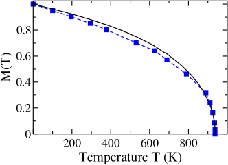
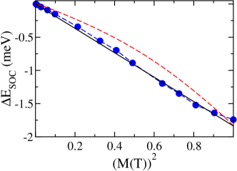
Figure 1: RDLM calculations on FePt. Top: the magnetization $M(T)$ versus $T$ for the magnetization along the easy [001] axis (filled squares). The full line shows the mean field approximation to a classical Heisenberg model for comparison. Bottom: the magnetic anisotropy energy $\Delta E_{\rm SOC}$ as a function of the square of the magnetization $M(T)$. The filled circles show the RDLM-based results, the full line give $K(T)\sim[M(T)/M(0)]^{2}$, and the dashed line is based on the single-ion model function. All data taken from Staunton et al. (2004).

I.2 Inter-atomic bilinear exchange interaction parameters

Most first-principles calculations on the bilinear exchange coupling parameters reported in the literature, are based on the magnetic force theorem (MFT) by evaluating the energy change due to a perturbation on the spin subsystem with respect to a suitable reference configuration Szilva et al. (2022). Many results are based on calculations of the spin-spiral energy $\epsilon(\vec{q})$, giving access to the exchange parameters in the momentum space, $J_{\vec{q}}$ Uhl et al. (1994); Halilov et al. (1998); Sandratskii and Bruno (2002); Heide et al. (2008), followed by a Fourier transformation to the real space representation $J_{ij}$. Alternatively, the real space exchange parameters are calculated directly by evaluating the energy change due to the tilting of spin moments of interacting atoms. The corresponding non-relativistic expression (so-called Liechtenstein or LKAG formula) has been implemented based on the KKR as well as LMTO Green function (GF) Liechtenstein et al. (1984, 1987); Pajda et al. (2000); Szilva et al. (2022) band structure methods. It should be noted that the magnetic force theorem provides a reasonable accuracy for the exchange coupling parameters in the case of infinitesimal rotations of the spins close to some equilibrium state, that can be justified only in the long wavelength and strong-coupling limits Solovyev (2021). Accordingly, calculations of the exchange coupling parameters beyond the magnetic force theorem, represented in terms of the inverse transverse susceptibility, were discussed in the literature by various authors Grotheer et al. (2001); Antropov (2003); Bruno (2003); Solovyev (2021); Szilva et al. (2022). Grotheer et al., for example, have demonstratedGrotheer et al. (2001) a deviation of the spin-wave dispersion curves away from $\Gamma$ point in the BZ, calculated for fcc Ni using the exchange parameters $\underline{J}_{\vec{q}}\sim\underline{\chi}^{-1}_{\vec{q}}$, from the MFT-based results for $\underline{J}_{\vec{q}}$. On the other hand, the results are close to each other in the long-wavelength limit (see Fig. 2).

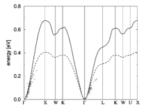
Figure 2: Adiabatic spin-wave dispersion relations along high-symmetry lines of the Brillouin zone for Ni. Broken line: frozen-magnon-torque method, full line: transverse susceptibility method Grotheer et al. (2001). All data are taken from Ref. Grotheer et al., 2001.

The calculations beyond the standard DFT are done by making use of the so-called constrained-field DFT. The latter theory was also used by Bruno Bruno (2003) who suggested the ’renormalization’ of the exchange coupling parameters expressed in terms of non-relativistic transverse magnetic susceptibility, according to $\underline{J}=\frac{1}{2}\underline{M}\underline{\chi}^{-1}\underline{M}=\frac{1}{2}\underline{M}(\underline{\tilde{\chi}}^{-1}-\underline{I}^{xc})\underline{M}$, with the various quantities defined as follows

$$\tilde{\chi}^{-1}_{ij} = \frac{2}{\pi}\int^{E_{F}}dE\,\int_{\Omega_{i}}d^{3}r\int_{\Omega_{j}}d^{3}r^{\prime}$$ (20)

$$\times\mbox{Im\,}[G^{\uparrow}(\vec{r},\vec{r}^{\prime},E)G^{\downarrow}(\vec{r}^{\prime},\vec{r},E)]\,,$$

$$M_{i} = \int_{\Omega_{i}}d^{3}r\,m(\vec{r})\,,$$ (21)

and

$$\tilde{I}^{xc}_{ij} = \delta_{ij}\frac{\Delta_{i}}{2M_{i}}\,,$$ (22)

with $\Delta_{i}=\frac{4}{M_{i}}\sum_{j}\tilde{J}_{ij}$, where

$$\tilde{J}_{ij} = \frac{1}{\pi}\mbox{Im\,}\int^{E_{F}}dE\,\int_{\Omega_{i}}d^{3}r\int_{\Omega_{j}}d^{3}r^{\prime}$$ (24)

$$\times[B_{xc}(\vec{r})G^{\uparrow}(\vec{r},\vec{r}^{\prime},E)B_{xc}(\vec{r}^{\prime})G^{\downarrow}(\vec{r}^{\prime},\vec{r},E)]\,.$$

This approach results in a Curie temperature of 634 K for fcc Ni (vs. 350 K based on the MFT) which is in good agreement with the experimental value of ($621-631$ K). As was pointed out by Solovyev Solovyev (2021), such a corrections can be significant only for a certain class of materials, while, for instance, the calculations of spin-wave energies Grotheer et al. (2001) and $T_{C}$ Bruno (2003) for bcc Fe demonstrate that these corrections are quite small. As most results in the literature were obtained using the exchange parameters based on the magnetic force theorem, we restrict below to this approximation.

Similar to the case of the MCA discussed above, application of the magnetic force theorem gives the energy change due to tilting of two spin moments represented in terms of the integrated DOS Liechtenstein et al. (1987). Within the multiple scattering formalism, this energy can be transformed using the Lloyd’s formula leading to the expression

$$\Delta{\cal E} = -\frac{1}{\pi}\mbox{Im\, Tr\,}\int^{E_{F}}dE\,\left(\mbox{ln}\,\underline{\underline{\tau}}(E)-\mbox{ln}\,\underline{\underline{\tau}}^{0}(E)\right)$$ (25)

with $\underline{\underline{\tau}}^{(0)}(E)$ and $\underline{\underline{\tau}}(E)$ the scattering path operators for non-distorted and distorted systems, respectively.

As reported in Ref. Liechtenstein et al., 1987, the expression for $J_{ij}$ representing the exchange interaction between the spin moments on sites $i$ and $j$, is given by the expression

$$J_{ij} = -\frac{1}{4\pi}\mathrm{ImTr_{L}}\int^{E_{F}}dE\underline{\Delta}_{i}\underline{\tau}^{\uparrow}_{ij}\underline{\Delta}_{j}\underline{\tau}^{\downarrow}_{ji}\;,$$ (26)

with $\underline{\Delta}_{i(j)}=([\underline{t}^{\uparrow}]^{-1}_{i(j)}-[\underline{t}^{\downarrow}]^{-1}_{i(j)})$, where $t^{\uparrow}_{i(j)}$ and $\underline{t}^{\downarrow}_{i(j)}$ are the spin-up and spin-down single-site scattering matrices, respectively, while $\underline{\tau}^{\uparrow}_{ij}$ and $\underline{\tau}^{\downarrow}_{ji}$ are the spin-up and spin-down, respectively, scattering path operators. As relativistic effects are not taken into account, the exchange interactions are isotropic with respect to the orientation of the magnetization as well as with respect to the direction of the spin tilting. On the other hand, spin-orbit coupling gives rise to an anisotropy for exchange interactions requiring a representation in the form of the exchange tensor $\underline{J}_{ij}$ with its antisymmetric part giving access to the Dzyaloshinskii-Moriya (DM) interaction $\vec{D}_{ij}$.

Udvardi et al. Udvardi et al. (2003) and later Ebert and Mankovsky Ebert and Mankovsky (2009) suggested an extension of the classical Heisenberg Hamiltonian by accounting for relativistic effects for the exchange coupling (see also Ref. Szilva et al., 2022). These calculations are based on a fully relativistic treatment of the electronic structure obtained by use of of the Dirac Hamiltonian

$${\cal H}_{\rm D} = -ic\vec{\alpha}\cdot\vec{\nabla}+\frac{1}{2}\,c^{2}(\beta-1)$$ (27)

$$\qquad+\bar{V}(\vec{r})+\beta\,\vec{\sigma}\cdot\vec{B}(\vec{r})+e\vec{\alpha}\cdot\vec{A}(\vec{r})\;.$$

Here, ${\alpha}_{i}$ and $\beta$ are the standard Dirac matrices Rose (1961) while $\bar{V}(\vec{r})$ and $\vec{B}(\vec{r})$ are the spin independent and spin dependent parts of the electronic potential.

Considering a ferromagnetic (FM) state as a reference state with the magnetization along the $z$ direction, a tilting of the magnetic moments on sites $i$ and $j$ leads to a modification of the scattering path operator implying the relation

$$\mbox{ln}\,\underline{\underline{\tau}}-\mbox{ln}\,\underline{\underline{\tau}}^{0} = -\mbox{ln}\left(1+\underline{\underline{\tau}}\,[\Delta{\underline{m}}_{i}+\Delta{\underline{m}}_{j}+...]\right)\;,$$ (28)

with ${\underline{m}}_{i}={\underline{t}}^{-1}_{i}$. This allows to write down the expression for the energy change due to a spin tilting on sites $i$ and $j$ as follows

$${\cal E}_{ij} = -\frac{1}{\pi}\mbox{Im\,Tr}\int^{E_{F}}dE\,\Delta m_{i}\,\tau_{ij}\,\Delta m_{j}\,\tau_{ji}$$ (29)

Within the approach of Udvardi et al. Udvardi et al. (2003), the dependence of the single-site inverse scattering matrix ${\underline{m}}_{i}$ on the orientation of magnetic moment $\hat{e}_{i}$ is accounted for by performing a corresponding rotation operation using the rotation matrix $\underline{R}(\theta,\phi)$, i.e., one has ${\underline{m}}_{i}(\theta,\phi)=\underline{R}(\theta,\phi){\underline{m}}^{0}_{i}\underline{R}^{+}(\theta,\phi)$. The change of the scattering matrix ${\underline{m}}_{i}$ under spin rotation, $\Delta{\underline{m}}_{i}$, linearized with respect to the rotation angles, is given by the expression

$$\Delta{\underline{m}}_{i} = \underline{R}(\theta_{i},\phi_{i})\underline{m}^{0}_{i}\underline{R}^{+}(\theta_{i},\phi_{i})-\underline{m}^{0}_{i}$$ (30)

$$= \underline{m}^{\theta}_{i}\delta\theta_{i}+\underline{m}^{\phi}_{i}\delta\phi_{i}$$

with

$$\underline{m}^{\theta}_{i} = \frac{\partial}{\partial\theta}\underline{m}_{i}=\frac{\partial R}{\partial\theta}\underline{m}_{i}R^{+}+R\underline{m}_{i}\frac{\partial R^{+}}{\partial\theta}\,,$$

$$\underline{m}^{\phi}_{i} = \frac{\partial}{\partial\phi}\underline{m}_{i}=\frac{\partial R}{\partial\phi}\underline{m}_{i}R^{+}+R\underline{m}_{i}\frac{\partial R^{+}}{\partial\phi}\,.$$ (31)

To calculate the derivatives of the rotation matrix, the definition

$$\hat{R}(\alpha_{\hat{n}},\hat{n}) = e^{i\alpha_{\hat{n}}(\hat{n}\cdot\hat{\vec{{J}}})}$$ (32)

for the corresponding operator is used, with $\hat{\vec{{J}}}$ the total angular momentum operator. $\hat{R}(\alpha_{\hat{n}},\hat{n})$ describes a rotation of the magnetic moment $\hat{m}$ by the angle $\alpha_{\hat{n}}$ about the direction $\hat{n}\perp\hat{m}$, that gives in particular $\underline{R}(\theta,\hat{n})$ for $\hat{n}=\hat{y}$ and $\underline{R}(\phi,\hat{n})$ for $\hat{n}=\hat{z}$.

This leads to the second derivatives of the total energy with respect to the titling angles $\alpha_{i}=\{\theta_{i},\phi_{i}\}$ and $\beta_{j}=\{\theta_{j},\phi_{j}\}$

$$\frac{\partial^{2}{\cal E}}{\partial\alpha_{i}\partial\beta_{j}} = -\frac{1}{\pi}\mbox{Im\,Tr}\int^{E_{F}}dE\underline{m}^{\alpha}_{i}\underline{\tau}_{ij}\underline{m}^{\beta}_{j}\underline{\tau}_{ji}$$ (33)

As is discussed by Udvardi et al. Udvardi et al. (2003), these derivatives give access to all elements $J^{\mu\nu}_{ij}$ of the exchange tensor, where $\mu(\nu)=\{x,y,z\}$. Note, however, that only the tensor elements with $\mu(\nu)=\{x,y\}$ can be calculated using the magnetization direction along the $\hat{z}$ axis, giving access to the $z$ component $D^{z}_{ij}$ of the DMI. In order to obtain all other tensor elements, an auxiliary rotation of the magnetization towards the $\hat{x}$ and $\hat{y}$ directions of the global frame of reference is required. For example, the component $D^{x}_{ij}$ if the DMI vector can be evaluated via the tensor elements

$$J^{zy}_{ij} = \frac{\partial^{2}E}{\partial\theta_{i}\partial\phi_{j}}\,\,\,\mbox{and}\,\,\,J^{yz}_{ij}=\frac{\partial^{2}F}{\partial\phi_{i}\partial\theta_{j}}$$ (34)

for $\theta=\frac{\pi}{2}$ and $\phi=0$.

An alternative expression within the KKR multiple scattering formalism has been worked out by Ebert and Mankovsky Ebert and Mankovsky (2009), by using the alternative convention for the electronic Green function (GF) as suggested by Dederichs and coworkers Dederichs et al. (1992). According to this convention, the off-site part of the GF is given by the expression:

$$G(\vec{r}_{i},\vec{r}_{j},E) = \sum_{\Lambda\Lambda^{\prime}}R^{i}_{\Lambda}(\vec{r}_{i},E)G^{ij}_{\Lambda\Lambda^{\prime}}(E)R^{j\times}_{\Lambda^{\prime}}(\vec{r}_{j},E)\;,$$ (35)

where $G^{ij}_{\Lambda\Lambda^{\prime}}(E)$ is the so-called structural Green’s function, $R^{i}_{\Lambda}$ is a regular solution to the single-site Dirac equation labeled by the combined quantum numbers $\Lambda$ Rose (1961). The energy change $\Delta{\cal E}_{ij}$ due to a spin tilting on sites $i$ and $j$ , given by Eq. (29), transformed to the above mentioned convention is expressed as follows

$$\Delta{\cal E}_{ij} = -\frac{1}{\pi}\mathrm{ImTr}\int dE\Delta\underline{t}^{i}\underline{G}^{ij}\Delta\underline{t}^{j}\underline{G}^{ji}\;,$$ (36)

where the change of the single-site t-matrix $\Delta\underline{t}^{i}$ can be represented in terms of the perturbation $\Delta V^{i}(\vec{r})$ at site $i$ using the expression

$$\Delta t_{\Lambda^{\prime}\Lambda}^{i} = \int d^{3}rR^{i\times}_{\Lambda^{\prime}}(r)\Delta V(r)R^{i}_{\Lambda}(r)=\Delta V_{\Lambda^{\prime}\Lambda}^{(R)i}\;,$$ (37)

where the perturbation caused by the rotation of the spin magnetic moment $\hat{e}_{i}$ is represented by a change of the spin-dependent potential in Eq. (27) (in contrast to the approach used in Ref. Udvardi et al., 2003)

$$\Delta V(r) = V_{\hat{n}}(r)-V_{\hat{n}_{0}}(r)=\beta\vec{\sigma}(\hat{n}-\hat{n}_{0})B(r)\;.$$ (38)

Using again the frozen potential approximation implies that the spatial part of the potential $V_{\hat{n}}(r)$ does not change upon rotation of spin orientation.

Coming back to the convention for the GF used by Györffy and coworkers Weinberger (1990) according to Eq. (9) the expression for the elements of the exchange tensor represented in terms of the scattering path operator $\tau^{ij}_{\Lambda^{\prime}\Lambda}(E)$ has the form

$$J_{ij}^{\alpha_{i}\alpha_{j}} = -\frac{1}{\pi}\mathrm{ImTr}\int dE\underline{T}^{\alpha_{i}}\underline{\tau}^{ij}\underline{T}^{\alpha_{j}}\underline{\tau}^{ji}\;,$$ (39)

where

$$T^{\alpha_{i}}_{\Lambda\Lambda^{\prime}} = \int d^{3}rZ^{\times}_{\Lambda}(\vec{r})\beta\sigma_{\alpha}B(r)Z_{\Lambda^{\prime}}(\vec{r})\;.$$ (40)

When compared to the approach of Udvardi et al.Udvardi et al. (2003), the expression in Eq. (39) is given explicitly in Cartesian coordinates. However, auxiliary rotations of the magnetization are still required to calculate all tensor elements, and as a consequence, all components of the DMI vector. This can be avoided using the approach reported recently Mankovsky et al. (2019) for DMI calculations.

In this case, using the grand-canonical potential in the operator form

$${\cal K} = {\cal H-\mu N}\;,$$ (41)

with $\mu$ the chemical potential, the variation of single-particle energy density $\Delta{\cal E}(\vec{r})$ caused by a perturbation is written in terms of the electronic Green function for $T=0$ K as follows

$$\Delta{\cal E}(\vec{r}) = -\frac{1}{\pi}\,\mbox{Im}\,\mbox{Tr}\int^{\mu}dE\,(E-\mu)\,\Delta G(\vec{r},\vec{r},E)\;.$$ (42)

Assuming the perturbation $\Delta V$ responsible for the change of the Green function $\Delta G=G-G_{0}$ (the index $0$ indicates here the collinear ferromagnetic reference state) to be small, $\Delta G$ can be expanded up to any order w.r.t. the perturbation

$$\Delta G(E) = G_{0}\Delta VG_{0}$$ (43)

$$+G_{0}\Delta VG_{0}\Delta VG_{0}$$

$$+G_{0}\Delta VG_{0}\Delta VG_{0}\Delta VG_{0}$$

$$+G_{0}\Delta VG_{0}\Delta VG_{0}\Delta VG_{0}\Delta VG_{0}+...\;,$$

leading to a corresponding expansion for the energy change with respect to the perturbation as follows

$$\Delta{\cal E} = \Delta{\cal E}^{(1)}+\Delta{\cal E}^{(2)}+\Delta{\cal E}^{(3)}+\Delta{\cal E}^{(4)}+...\;,$$ (44)

Here and below we drop the energy argument for the Green function $G(E)$ for the sake of convenience. This expression is completely general as it gives the energy change as a response to any type of perturbation. When $\Delta V$ is associated with tiltings of the spin magnetic moments, it can be expressed within the frozen potential approximation and in line with Eq. (38) as follows

$$\Delta V(\vec{r}) = \sum_{i}\beta\big{(}\vec{\sigma}\cdot\hat{s}_{i}-\sigma_{z}\big{)}B_{xc}(\vec{r})\;.$$ (45)

With this, the energy expansion in Eq (44) gives access to the bilinear DMI as well as to higher order multispin interactions Mankovsky et al. (2020). To demonstrate the use of this approach, we start with the $x$ and $y$ components of the DMI vector, which can be obtained by setting the perturbation $\Delta V$ in the form of a spin-spiral described by the configuration of the magnetic moments

$$\hat{m}_{i}=\Big{(}\sin(\vec{q}\cdot\vec{R}_{i}),0,\cos(\vec{q}\cdot\vec{R}_{i})\Big{)}\;,$$ (46)

with the wave vector $\vec{q}=(0,q,0)$. As it follows from the spin Hamiltonian, the slope of the spin wave energy dispersion at the $\Gamma$ point is determined by the DMI as follows

$$\lim_{q\to 0}\frac{\partial E_{\rm DM}^{(1)}}{\partial q_{y}} = \lim_{q\to 0}\frac{\partial}{\partial q_{y}}\sum_{ij}D^{y}_{ij}\,\sin(\vec{q}\cdot(\vec{R}_{j}-\vec{R}_{i}))$$ (47)

$$= \sum_{ij}D^{y}_{ij}\,(\vec{R}_{j}-\vec{R}_{i})_{y}\;.$$

Identifying this with the corresponding derivative of the energy $\Delta{\cal E}^{(1)}$ in Eq. 44

$$\frac{\partial\Delta{\cal E}^{(1)}}{\partial q_{\alpha}}\bigg{|}_{q\to 0}=\frac{\partial E_{\rm DM}^{(1)}}{\partial q_{\alpha}}\bigg{|}_{q\to 0}\;,$$ (48)

and equating the corresponding terms for each atomic pair $(i,j)$, one obtains the following expression for the $y$ component of the DMI vector:

$$D^{y}_{ij} = \left(-\frac{1}{2\pi}\right)\mbox{Im}\,\mbox{Tr}\int^{\mu}dE\,(E-\mu)$$ (49)

$$\times \bigg{[}{\underline{O}^{j}(E)}\,\underline{\tau}^{ji}(E)\,{\underline{T}^{i,x}(E)}\,\underline{\tau}^{ij}(E)$$

$$-{\underline{O}^{i}(E)}\,\underline{\tau}^{ij}(E)\,{\underline{T}^{j,x}(E)}\,\underline{\tau}^{ji}(E)\bigg{]}\;,$$

In a completely analogous way one can derive the x-component of the DMI vector, $D^{x}_{ij}$. The overlap integrals $O^{j}_{\Lambda\Lambda^{\prime}}$ and matrix elements $T^{i,\alpha}_{\Lambda\Lambda^{\prime}}$ of the operator ${\cal T}^{i,\alpha}=\beta\sigma_{\alpha}B_{xc}^{i}(\vec{r})$ (which are connected with the components of the torque operator $\beta[\vec{\sigma}\times\hat{m}]B^{i}_{xc}(\vec{r})$) are defined as follows:Ebert and Mankovsky (2009)

$$O^{j}_{\Lambda\Lambda^{\prime}} = \int_{\Omega_{j}}d^{3}r\,Z^{j\times}_{\Lambda}(\vec{r},E)\,Z^{j}_{\Lambda^{\prime}}(\vec{r},E)$$ (50)

$$T^{i,\alpha}_{\Lambda\Lambda^{\prime}} = \int_{\Omega_{i}}d^{3}r\,Z^{i\times}_{\Lambda}(\vec{r},E)\,\Big{[}\beta\sigma_{\alpha}B_{xc}^{i}(\vec{r})\Big{]}\,Z^{i}_{\Lambda^{\prime}}(\vec{r},E)\;.$$ (51)

As is shown in Ref. Mankovsky et al., 2020, the $D_{ij}^{z}$ component of the DMI, as well isotropic exchange parameter $J_{ij}$ can also be obtained on the basis of Eqs. (43) and (44) using the second order term w.r.t. the perturbation, for a spin spiral with the form

$$\hat{s}_{i} = (\sin\theta\cos(\vec{q}\cdot\vec{R}),\sin\theta\sin(\vec{q}\cdot\vec{R}),\cos\theta)\,.$$ (52)

In this case case, the DMI component $D^{z}_{ij}$ and the isotropic exchange interaction are obtained by taking the first- and second-order derivatives of the energy $\Delta{\cal E}^{(2)}(\vec{q})$ (see Eq. (44)), respectively, with respect to $\vec{q}$:

$$\frac{\partial}{\partial\vec{q}}\Delta E_{H}(\vec{q})\bigg{|}_{q\to 0} = -\sin^{2}\theta\sum_{i\neq j}^{N}D^{z}_{ij}\hat{q}\cdot(\vec{R}_{i}-\vec{R}_{j})$$ (53)

and

$$\frac{\partial^{2}}{\partial\vec{q}^{2}}\Delta E_{H}(\vec{q})\bigg{|}_{q\to 0} = \sin^{2}\theta\sum_{i,j}J_{ij}(\hat{q}\cdot(\vec{R}_{i}-\vec{R}_{j}))^{2}$$ (54)

with $\hat{q}=\vec{q}/|\vec{q}|$ the unit vector giving the direction of the wave vector $\vec{q}$. Identifying these expressions again with the corresponding derivatives of $\Delta{\cal E}^{(2)}(\vec{q})$, one obtains the following relations for $D^{z}_{ij}$

$$D^{z}_{ij} = \frac{1}{2}({\cal J}^{xy}_{ij}-{\cal J}^{yx}_{ij})$$ (55)

and for $J_{ij}$

$$J_{ij} = \frac{1}{2}({\cal J}^{xx}_{ij}+{\cal J}^{yy}_{ij})\,,$$ (56)

where the tensor elements ${\cal J}^{\alpha\beta}$ are given by Eqs. (39) and (40).

Similar to the magnetic anisotropy, the exchange coupling parameters depend on temperature, that should be taken into account within the finite temperature spin dynamic simulations. An approach that gives access to calculations of exchange coupling parameters for finite temperature has been reported in Ref. Mankovsky et al., 2020. It accounts for the electronic structure modification due to temperature induced lattice vibrations by using the alloy analogy model in the adiabatic approximation. This implies calculations of the thermal average $\langle...\rangle_{T}$ as the configurational average over a set of appropriately chosen set of atomic displacements, using the CPA alloy theory Ebert et al. (2011b); Mankovsky et al. (2013); Ebert et al. (2015).

To make use of this scheme to account for lattice vibrations, a discrete set of $N_{v}$ vectors $\Delta\vec{R}^{q}_{v}(T)$ is introduced for each atom, with the temperature dependent amplitude, which characterize a rigid displacement of the atomic potential in the spirit of the rigid muffin-tin approximation Papanikolaou et al. (1997); Lodder (1976). The corresponding single-site t-matrix in the common global frame of the solid is given by the transformation:

$$\underline{t}^{q}_{v}=\underline{U}(\Delta\vec{R}_{v})\,\underline{t}^{q,\rm loc}\,\underline{U}(\Delta\vec{R}_{v})^{-1}\;,$$ (57)

with the so-called U-transformation matrix $\underline{U}(\vec{s})$ given in its non-relativistic form by:Lodder (1976); Papanikolaou et al. (1997)

$$U_{LL^{\prime}}(\vec{s})=4\pi\sum_{L^{\prime\prime}}i^{l+l^{\prime\prime}-l^{\prime}}\,C_{LL^{\prime}L^{\prime\prime}}\,j_{l^{\prime\prime}}(|\vec{s}|k)\,Y_{L^{\prime\prime}}(\hat{s})\;.$$ (58)

Here $L=(l,m)$ represents the non-relativistic angular momentum quantum numbers, $j_{l}(x)$ is a spherical Bessel function, $Y_{L}(\hat{r})$ a real spherical harmonics, $C_{LL^{\prime}L^{\prime\prime}}$ a corresponding Gaunt number and $k=\sqrt{E}$ is the electronic wave vector. The relativistic version of the U-matrix is obtained by a standard Clebsch-Gordan transformation.Rose (1961)

Every displacement characterized by a displacement vectors $\Delta\vec{R}_{v}(T)$ can be treated as a pseudo-component of a pseudo alloy. Thus, the thermal averaging can be performed as the site diagonal configurational average for a substitutional alloy, by solving the multi-component CPA equations within the global frame of reference Ebert et al. (2015).

The same idea can be used also to take into account thermal spin fluctuations. A set of representative orientation vectors $\hat{e}_{f}$ (with $f=1,...,N_{f}$) for the local magnetic moment is introduced. Using the rigid spin approximation, the single-site t-matrix in the global frame, corresponding to a given orientation vector, is determined by:

$$\underline{t}^{q}_{f}=\underline{R}(\hat{e}_{f})\,\underline{t}^{q,\rm loc}\,\underline{R}(\hat{e}_{f})^{-1}\;,$$ (59)

where $\underline{t}^{q,\rm loc}$ is the single-site t-matrix in the local frame. Here the transformation from the local to the global frame of reference is expressed by the rotation matrices $\underline{R}(\hat{e}_{f})$ that are determined by the vectors $\hat{e_{f}}$ or corresponding Euler angles.Rose (1961) Again, every orientation can be treated as a pseudo-component of a pseudo alloy, that allows to use the alloy analogy model to calculate the thermal average over all types of spin fluctuations Ebert et al. (2015).

The alloy analogy for thermal vibrations applied to the temperature dependent exchange coupling parameters leads to

$$\bar{J}_{ij}^{\alpha_{i}\alpha_{j}} = -\frac{1}{2\pi}\Im\int dE\,\mathrm{Trace}\langle\Delta\underline{V}^{\alpha_{i}}\underline{\tau}^{ij}\Delta\underline{V}^{\alpha_{j}}\underline{\tau}^{ji}\rangle_{c}\;,$$ (60)

where $\langle...\rangle_{\rm c}$ represents the configurational average with respect to the set of displacements. In case of the exchange coupling parameters one has to distinguish between the averaging over thermal lattice vibrations and spin fluctuations. In the first case the configurational average is approximated as follows $\langle\Delta\underline{V}^{i}\underline{\tau}^{ij}\Delta\underline{V}^{j}\underline{\tau}^{ji}\rangle_{vib}\approx\langle\Delta\underline{V}^{i}\underline{\tau}^{ij}\rangle_{vib}\langle\Delta\underline{V}^{j}\underline{\tau}^{ji}\rangle_{vib}$, assuming a negligible impact of the so-called vertex corrections Butler (1985). This averaging accounts for the impact of thermally induced phonons on the exchange coupling parameters for every temperature before their use in MC or spin dynamics simulations that deal subsequently with the thermal averaging in spin subspace. The impact of spin fluctuations can be incorporated as well within the electronic structure calculations. For a non-polarized paramagnetic reference state, this can be done, e.g., by using the so-called disorder local moment (DLM) scheme formulated in general within the non-relativistic (or scalar-relativistic) framework. Magnetic disorder in this case can be modeled by creating a pseudo alloy with an occupation of the atomic sites by two types of atoms with opposite spin moments oriented upwards, $M^{\uparrow}$ and downwards $M^{\downarrow}$, respectively, i.e. considering the alloy $M_{0.5}^{\uparrow}M_{0.5}^{\downarrow}$. In the relativistic case the corresponding RDLM scheme has to describe the magnetic disorder by a discrete set of $N_{f}$ orientation vectors, and as a consequence, the average $\langle\underline{\tau}^{ij}\rangle_{spin}$ has to be calculated taking into account all these orientations. A comparison of the results obtained for the isotropic exchange coupling constants $J_{ij}$ for bcc Fe using the DLM and RDLM schemes is shown in Fig. 3, demonstrating close agreement, with the small differences to be ascribed to the different account of relativistic effects, i.e. in particular the spin-orbit coupling.

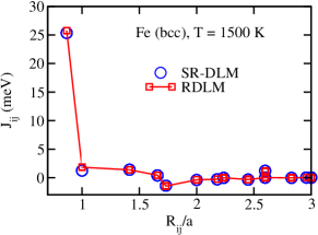
Figure 3: Isotropic exchange coupling parameters calculated for the disordered magnetic state of bcc Fe within the scalar-relativistic approach, using the DLM scheme (circles, SR-DLM) and within the fully-relativistic approach, using the RDLM scheme Staunton et al. (2004, 2006) (squares, RDLM).

I.3 Multi-spin expansion of spin Hamiltonian: General remarks

Despite the obvious success of the classical Heisenberg model for many applications, higher-order multi-spin expansion $H_{ms}$ of the spin Hamiltonian $H$, given by the expression

$$H_{ms} = -\frac{1}{3!}\sum_{i,j,k}J_{ijk}\hat{s}_{i}\cdot(\hat{s}_{j}\times\hat{s}_{k})\;,$$ (61)

$$-\frac{2}{p!}\sum_{i,j,k,l}J^{s}_{ijkl}(\hat{s}_{i}\cdot\hat{s}_{j})(\hat{s}_{k}\cdot\hat{s}_{l})$$

$$-\frac{2}{p!}\sum_{i,j,k,l}\vec{{\cal D}}_{ijkl}\cdot(\hat{s}_{i}\times\hat{s}_{j})(\hat{s}_{k}\cdot\hat{s}_{l})+...\;,$$

$$= H^{3}+H^{4,s}+H^{4,a}+...$$

can be of great importance to describe more subtle properties of magnetic materials Harris and Owen (1963); Huang and Orbach (1964); Allan and Betts (1967); Iwashita and Uryâ (1974); Iwashita and Uryû (1976); Aksamit (1980); Brown (1984); Ivanov et al. (2014); Antal et al. (2008); Müller-Hartmann et al. (1997); Greiter and Thomale (2009); Greiter et al. (2014); Fedorova et al. (2015).

This concerns first of all systems with a non-collinear ground state characterized by finite spin tilting angles, that makes multispin contributions to the energy non-negligible. In particular, many reports published recently discuss the impact of the multispin interactions on the stabilization of exotic topologically non-trivial magnetic textures, e.g. skyrmions, hopfions, etc. Mendive-Tapia et al. (2021); Gutzeit et al. (2021); Hayami (2022)

Corresponding calculations of the multi-spin exchange parameters have been reported by different groups. The approach based on the Connolly-Williams scheme has been used to calculate the four-spin non-chiral (two-site and three-site) and chiral interactions for Cr trimers Antal et al. (2008) and for a deposited Fe atomic chain Lászlóffy et al. (2019), respectively, for the biquadratic, three-site four spin and four-site four spin interaction parameters Paul et al. (2020); Gutzeit et al. (2021). The authors discuss the role of these type of interactions for the stabilization of different types of non-collinear magnetic structures as skyrmions and antiskyrmions.

A more flexible mapping scheme using perturbation theory within the KKR Green function formalism was only reported recently by Brinker et al. Brinker et al. (2019, 2020), and by the present authors Mankovsky et al. (2020). Here we discuss the latter approach, i.e. the energy expansion w.r.t. $\Delta V$ in Eq. (44). One has to point out that a spin tilting in a real system has a finite amplitude and therefore the higher order terms in this expansion might become non-negligible and in general should be taken into account. Their role obviously depends on the specific material and should increase with temperature that leads to an increasing amplitude of the spin fluctuations. As these higher-order terms are directly connected to the multispin terms in the extended Heisenberg Hamiltonian, one has to expect also a non-negligible role of the multispin interactions for some magnetic properties.

Extending the spin Hamiltonian to go beyond the classical Heisenberg model, we discuss first the four-spin exchange interaction terms $J_{ijkl}$ and $\vec{\cal D}_{ijkl}$. They can be calculated using the fourth-order term of the Green function expansion $\Delta{\cal E}^{(4)}$ given by:

$$\Delta{\cal E}^{(4)} = -\frac{1}{\pi}\mbox{Im}\,\mbox{Tr}\int^{E_{F}}dE\,$$

$$\times(E-E_{F})\Delta VG\Delta VG\Delta VG\Delta VG$$

$$= -\frac{1}{\pi}\mbox{Im}\,\mbox{Tr}\int^{E_{F}}dE\,\Delta VG\Delta VG\Delta VG\Delta VG\;.$$

where the sum rule for the Green function $\frac{dG}{dE}=-GG$ followed by integration by parts was used to get a more compact expression. Using the multiple-scattering representation for the Green function, this leads to:

$$\Delta{\cal E}^{(4)} = \sum_{i,j,k,l}-\frac{1}{\pi}\mbox{Im}\,\mbox{Tr}\int^{E_{F}}dE\,$$ (63)

$$\times\Delta\underline{V}_{ii}\underline{\tau}_{ij}\Delta\underline{V}_{jj}\underline{\tau}_{jk}\Delta\underline{V}_{kk}\underline{\tau}_{kl}\Delta\underline{V}_{ll}\underline{\tau}_{li}\;.$$

with the matrix elements $\Delta\underline{V}_{ii}=\langle Z_{i}|\Delta V|Z_{i}\rangle$. Using the ferromagnetic state with $\vec{M}||\hat{z}$ as a reference state, and creating the perturbation $\Delta V$ in the form of a spin-spiral according to Eq. (52), one obtains the corresponding $\vec{q}$-dependent energy change $\Delta{\cal E}^{(4)}(\vec{q})$, written here explicitly as an example

$$\Delta{\cal E}^{(4)} = -\frac{1}{\pi}\sum_{i,j,k,l}\mbox{Im}\,\mbox{Tr}\int^{E_{F}}dE\,\mbox{sin}^{4}\theta$$

$$\times\bigg{[}I^{xxxx}_{ijkl}\;\mbox{cos}(\vec{q}\cdot\vec{R}_{i})\,\mbox{cos}(\vec{q}\cdot\vec{R}_{j})\,\mbox{cos}(\vec{q}\cdot\vec{R}_{k})\,\mbox{cos}(\vec{q}\cdot\vec{R}_{l})$$

$$+I^{xxyy}_{ijkl}\;\mbox{cos}(\vec{q}\cdot\vec{R}_{i})\,\mbox{cos}(\vec{q}\cdot\vec{R}_{j})\,\mbox{sin}(\vec{q}\cdot\vec{R}_{k})\,\mbox{sin}\vec{q}\cdot\vec{R}_{l})$$

$$+I^{yyxx}_{ijkl}\;\mbox{sin}(\vec{q}\cdot\vec{R}_{i})\,\mbox{sin}(\vec{q}\cdot\vec{R}_{j})\,\mbox{cos}(\vec{q}\cdot\vec{R}_{k})\,\mbox{cos}(\vec{q}\cdot\vec{R}_{l})$$

$$+I^{yyyy}_{ijkl}\;\mbox{sin}(\vec{q}\cdot\vec{R}_{i})\,\mbox{sin}(\vec{q}\cdot\vec{R}_{j})\,\mbox{sin}(\vec{q}\cdot\vec{R}_{k})\,\mbox{sin}(\vec{q}\cdot\vec{R}_{l})$$

$$+I^{xyxx}_{ijkl}\;\mbox{cos}(\vec{q}\cdot\vec{R}_{i})\,\mbox{sin}(\vec{q}\cdot\vec{R}_{j})\,\mbox{cos}(\vec{q}\cdot\vec{R}_{k})\,\mbox{cos}(\vec{q}\cdot\vec{R}_{l})$$

$$+I^{yxyy}_{ijkl}\;\mbox{sin}(\vec{q}\cdot\vec{R}_{i})\,\mbox{cos}(\vec{q}\cdot\vec{R}_{j})\,\mbox{sin}(\vec{q}\cdot\vec{R}_{k})\,\mbox{sin}\vec{q}\cdot\vec{R}_{l})$$

$$+I^{yxxx}_{ijkl}\;\mbox{sin}(\vec{q}\cdot\vec{R}_{i})\,\mbox{cos}(\vec{q}\cdot\vec{R}_{j})\,\mbox{cos}(\vec{q}\cdot\vec{R}_{k})\,\mbox{cos}(\vec{q}\cdot\vec{R}_{l})$$

$$+I^{xyyy}_{ijkl}\;\mbox{cos}(\vec{q}\cdot\vec{R}_{i})\,\mbox{sin}(\vec{q}\cdot\vec{R}_{j})\,\mbox{sin}(\vec{q}\cdot\vec{R}_{k})\,\mbox{sin}(\vec{q}\cdot\vec{R}_{l})+...\bigg{]}$$

where

$$I^{\alpha\beta\gamma\delta}_{ijkl} = \underline{T}^{i,\alpha}(E)\,\underline{\tau}^{ij}(E)\underline{T}^{j,\beta}(E)\,\underline{\tau}^{jk}(E)$$ (65)

$$\times\underline{T}^{k,\gamma}(E)\,\underline{\tau}^{kl}(E)\underline{T}^{l,\delta}(E)\,\underline{\tau}^{li}(E)\;.$$

As is shown in Ref. Mankovsky et al., 2020, the four-spin isotropic exchange interaction $J_{ijkl}$ and $z$-component of the DMI-like interaction ${\cal D}^{z}_{ijkl}$ can be obtained calculating the energy derivatives $\frac{\partial^{4}}{\partial q^{4}}\Delta{\cal E}^{(4)}$ and $\frac{\partial^{3}}{\partial q^{3}}\Delta{\cal E}^{(4)}$ in the limit of $q=0$, and then identified with the corresponding derivatives of the terms $H^{4,s}$ and $H^{4,a}$ in Eq. (61). These interaction terms are given by the expressions

$$J_{ijkl}^{s} = \frac{1}{4}\bigg{[}{\cal J}_{ijkl}^{xxxx}+{\cal J}_{ijkl}^{xxyy}+{\cal J}_{ijkl}^{yyxx}+{\cal J}_{ijkl}^{yyyy}\bigg{]}$$ (66)

and

$$D_{ijkl}^{z} = \frac{1}{4}\bigg{[}{\cal J}_{ijkl}^{xyxx}+{\cal J}_{ijkl}^{xyyy}-{\cal J}_{ijkl}^{yxxx}-{\cal J}_{ijkl}^{yxyy})\;\bigg{]}\,,$$ (67)

where the following definition is used:

$${\cal J}_{ijkl}^{\alpha\beta\gamma\delta} = \frac{1}{2\pi}\mbox{Im}\,\mbox{Tr}\int^{E_{F}}dE\,T^{\alpha}_{i}\tau_{ij}T^{\beta}_{j}\tau_{jk}T^{\gamma}_{k}\tau_{kl}T^{\delta}_{l}\tau_{li}$$ (68)

These expression obviously give also access to a special cases, i.e. the four-spin three-site interactions with $l=j$, and the four spin two-site, so called biquadratic exchange interactions with $k=i$ and $l=j$.

The scalar biquadratic exchange interaction parameters $J^{s}_{ijij}$ calculated on the basis of Eq. (66) for the three $3d$ bulk ferromagnetic systems bcc Fe, hcp Co and fcc Ni have been reported in Ref. Mankovsky et al., 2020. The results are plotted in Fig. 4 as a function of the distance $R_{ij}+R_{jk}+R_{kl}+R_{li}$. For comparison, the insets give the corresponding bilinear isotropic exchange interactions for these materials. One can see rather strong first-neighbor interactions for bcc Fe, demonstrating the non-negligible character of the biquadratic interactions. This is of course a material-specific property, and one notes as decrease for the biquadratic exchange parameters when going to Co and Ni as shown in Fig. 4 (b) and (c), respectively.

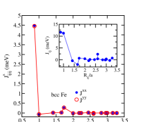
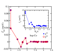
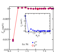
(a)  (b)  (c)

Figure 4: Scalar biquadratic exchange interactions $J^{s}_{ijij}$ in bcc Fe (a), hcp Co (b) and fcc Ni (Ni). For comparison, the insets show the bilinear exchange interaction parameters calculated for the FM state with the magnetization along the $\hat{z}$-axis. All data are taken from Ref. Mankovsky et al., 2020.

In order to calculate the $x$ and $y$ components of the four-spin and as a special case the three-site-DMI (TDMI) and biquadratic-DMI (BDMI) type interactions, the scheme suggested in Ref. Mankovsky et al., 2020 for the calculation of the DMI parameters Mankovsky and Ebert (2017); Mankovsky et al. (2019) can be used, which exploited the DMI-governed behavior of the spin-wave dispersion having a finite slope at the $\Gamma$ point of the Brillouin zone. Note, however, that a more general form of perturbation is required in this case described by a 2D spin modulation field according to the expression

$$\hat{s}_{i} = \big{(}\mbox{sin}(\vec{q}_{1}\cdot\vec{R}_{i})\;\mbox{cos}(\vec{q}_{2}\cdot\vec{R}_{i}),\mbox{sin}(\vec{q}_{2}\cdot\vec{R}_{i}),$$ (69)

$$\mbox{cos}(\vec{q}_{1}\cdot\vec{R}_{i})\mbox{cos}(\vec{q}_{2}\cdot\vec{R}_{i})\big{)}\;,$$

where the wave vectors $\vec{q}_{1}$ and $\vec{q}_{2}$ are orthogonal to each other, as for example $\vec{q}_{1}=q_{1}\hat{y}$ and $\vec{q}_{2}=q_{2}\hat{x}$.

Taking the second-order derivative with respect to the wave-vector $\vec{q}_{2}$ and the first-order derivative with respect to the wave-vectors $\vec{q}_{1}$ and $\vec{q}_{2}$, and considering the limit $q_{1(2)}\to 0$, one obtains

$$\frac{\partial^{3}}{\partial q_{2}^{3}}\bigg{|}_{q_{2}=0}{H}^{4,a} = \sum_{i,j,k,l}{\cal D}^{x}_{ijkl}\,({\hat{q}_{2}}\cdot\vec{R}_{ij})\,({\hat{q}_{2}}\cdot\vec{R}_{lk})^{2}\,,$$

and

$$\frac{\partial}{\partial q_{1}}\bigg{|}_{q_{1}=0}\frac{\partial^{2}}{\partial q_{2}^{2}}\bigg{|}_{q_{2}=0}{H}^{4,a} = \sum_{i,j,k,l}{\cal D}^{y}_{ijkl}\,({\hat{q}_{1}}\cdot\vec{R}_{ij})\,({\hat{q}_{2}}\cdot\vec{R}_{lk})^{2}\,,$$

where $\vec{R}_{ij}=\vec{R}_{j}-\vec{R}_{i}$ and $\vec{R}_{lk}=\vec{R}_{k}-\vec{R}_{l}$.

The microscopic expressions for the $x$ and $y$ components of $\vec{\cal D}_{ijkl}$ describing the four-spin interactions is derived on the basis of the third-order term in Eq. (43)

$$\Delta{\cal E}^{(3)} = -\frac{1}{\pi}\mbox{Im}\,\mbox{Tr}\int^{E_{F}}dE(E-E_{F})\,$$ (70)

$$\times G_{0}\Delta VG_{0}\Delta VG_{0}\Delta VG_{0}\;.$$

The final expression for ${\cal D}^{\alpha}_{ijkl}$ is achieved by taking the second-order derivative with respect to the wave-vector $\vec{q}_{2}$ and the first-order derivative with respect to the wave-vectors $\vec{q}_{1(2)}$, considering the limit $q_{1(2)}\to 0$, i.e. equating within the ab-initio and model expressions the corresponding terms proportional to $({\vec{R}}_{i}-{\vec{R}}_{j})_{y}({\vec{R}}_{k}-{\vec{R}}_{l})^{2}_{x}$ and $({\vec{R}}_{i}-{\vec{R}}_{j})_{x}({\vec{R}}_{k}-{\vec{R}}_{l})^{2}_{x}$ (we keep a similar form in both cases for the sake of convenience) gives the elements ${\cal D}^{y,x}_{ijkl}$ and ${\cal D}^{y,y}_{ijkl}$, as well as ${\cal D}^{x,x}_{ijkl}$ and ${\cal D}^{x,y}_{ijkl}$, respectively, of the four-spin chiral interaction as follows

$${\cal D}^{\alpha,\beta}_{ijkj} = \epsilon_{\alpha\gamma}\frac{1}{8\pi}\mbox{Im}\,\mbox{Tr}\int^{E_{F}}dE(E-E_{F})\,$$ (71)

$$\Big{[}\underline{O}^{i}\,\underline{\tau}^{ij}\underline{T}^{j,\gamma}\,\underline{\tau}^{jk}\underline{T}^{k,\beta}\,\underline{\tau}^{kl}\underline{T}^{l,\beta}\,\underline{\tau}^{li}\;$$

$$-\underline{T}^{i,\gamma}\,\underline{\tau}^{ij}\underline{O}^{j}\underline{\tau}^{jk}\underline{T}^{k,\beta}\,\underline{\tau}^{kl}\underline{T}^{l,\beta}\,\underline{\tau}^{li}\Big{]}\;\,$$

$$+\Big{[}\underline{O}^{i}\,\underline{\tau}^{ij}\underline{T}^{j,\beta}\,\underline{\tau}^{jk}\underline{T}^{k,\beta}\,\underline{\tau}^{kl}\underline{T}^{l,\gamma}\,\underline{\tau}^{li}\;$$

$$-\underline{T}^{i,\gamma}\,\underline{\tau}^{ij}\underline{T}^{j,\beta}\underline{\tau}^{jk}\underline{T}^{k,\beta}\,\underline{\tau}^{kl}\underline{O}^{l}\,\underline{\tau}^{li}\Big{]}\;$$

with $\alpha,\beta=x,y$, and $\epsilon_{\alpha\gamma}$ the elements of the transverse Levi-Civita tensor $\underline{\epsilon}=\begin{bmatrix}0&1\\ -1&0\end{bmatrix}$. The TDMI and BDMI parameters can be obtained as the special cases $l=j$ and $l=j,k=i$, respectively, from Eq. (71).

The expression in Eq. (71) gives access to the $x$ and $y$ components of the DMI-like three-spin interactions

$${\cal D}^{\alpha}_{ijkj}={\cal D}^{\alpha,x}_{ijkj}+{\cal D}^{\alpha,y}_{ijkj}\;.$$ (72)

Finally, three-spin chiral exchange interaction (TCI) represented by first term in the extended spin Hamiltonian has been discussed in Ref. Mankovsky et al., 2020. As it follows from this expression, the contribution due to this type of interaction is non-zero only in case of a non-co-planar and non-collinear magnetic structure characterized by the scalar spatial type product $\hat{s}_{i}\cdot(\hat{s}_{j}\times\hat{s}_{k})$ involving the spin moments on three different lattice sites.

In order to work out the expression for the $J_{ijk}$ interaction, one has to use a multi-Q spin modulation Solenov et al. (2012); Okubo et al. (2012); Batista et al. (2016) which ensure a non-zero scalar spin chirality for every three atoms. The energy contribution due to the TCI, is non-zero only if $J_{ijk}\neq J_{ikj}$, etc. Otherwise, the terms $ijk$ and $ikj$ cancel each other due to the relation $\hat{s}_{i}\cdot(\hat{s}_{j}\times\hat{s}_{k})=-\hat{s}_{i}\cdot(\hat{s}_{k}\times\hat{s}_{j})$.

Accordingly, the expression for the TCI is derived using the 2Q non-collinear spin texture described by Eq. (69), which is characterized by two wave vectors oriented along two mutually perpendicular directions, as for example $\vec{q}_{1}=(0,q_{y},0)$ and $\vec{q}_{2}=(q_{x},0,0)$. Applying such a spin modulation in Eq. (69) for the term $H^{3}$ associated with the three-spin interaction in the spin Hamiltonian in Eq. (61), the second-order derivative of the energy $E^{(3)}(\vec{q}_{1},\vec{q}_{2})$ with respect to the wave vectors $q_{1}$ and $q_{2}$ is given in the limit $q_{1}\to 0$, $q_{2}\to 0$ by the expression

$$\frac{\partial^{2}}{\partial\vec{q}_{1}\partial\vec{q}_{2}}H^{(3)}$$

$$=-\sum_{i\neq j\neq k}J_{ijk}\big{(}\hat{z}\cdot[(\vec{R}_{i}-\vec{R}_{j})\times(\vec{R}_{k}-\vec{R}_{j})]\big{)}\;.$$ (73)

The microscopic energy term of the electron system, giving access to the chiral three-spin interaction in the spin Hamiltonian is described by the second-order term

$$\Delta{\cal E}^{(2)} = -\frac{1}{\pi}\mbox{Im}\,\mbox{Tr}\int^{E_{F}}dE(E-E_{F})\,$$ (74)

$$G_{0}\Delta VG_{0}\Delta VG_{0}\;$$

of the free energy expansion. Taking the first-order derivative with respect to $q_{1}$ and $q_{2}$ in the limit $q_{1}\to 0$, $q_{2}\to 0$, and equating the terms proportional to $\big{(}\hat{z}\cdot[(\vec{R}_{i}-\vec{R}_{j})\times(\vec{R}_{k}-\vec{R}_{j})]\big{)}$ with the corresponding terms in the spin Hamiltonian, one obtains the following expression for the three-spin interaction parameter

$$J_{ijk} = \frac{1}{8\pi}\mbox{Im}\,\mbox{Tr}\int^{E_{F}}dE(E-E_{F})\,$$ (75)

$$\Big{[}\underline{T}^{i,x}\,\underline{\tau}^{ij}\underline{T}^{j,y}\,\underline{\tau}^{jk}\underline{O}^{k}\,\underline{\tau}^{ki}-\underline{T}^{i,y}\,\underline{\tau}^{ij}\underline{T}^{j,x}\,\underline{\tau}^{jk}\underline{O}^{k}\,\underline{\tau}^{ki}$$

$$-\underline{T}^{i,x}\,\underline{\tau}^{ij}\underline{O}^{j}\,\underline{\tau}^{jk}\underline{T}^{k,y}\,\underline{\tau}^{ki}\;+\underline{T}^{i,y}\,\underline{\tau}^{ij}\underline{O}^{j}\,\underline{\tau}^{jk}\underline{T}^{k,x}\,\underline{\tau}^{ki}\;$$

$$+\underline{O}^{i}\,\underline{\tau}^{ij}\underline{T}^{i,x}\,\underline{\tau}^{jk}\underline{T}^{k,y}\,\underline{\tau}^{ki}\;-\underline{O}^{j}\,\underline{\tau}^{ij}\underline{T}^{i,y}\,\underline{\tau}^{jk}\underline{T}^{k,x}\,\underline{\tau}^{ki}\Big{]}\;,$$

giving access to the three-spin chiral interaction determined as $J_{\Delta}=J_{ijk}-J_{ikj}$. Its interpretation was discussed in Ref. Mankovsky et al., 2021, where its dependence on the SOC as well as on the topological orbital susceptibility $\chi_{\Delta}^{TO}=\chi_{ijk}^{TO}-\chi_{ikj}^{TO}$ was demonstrated. In fact that the expression for $\chi_{ijk}^{TO}$ worked out in Ref. Mankovsky et al., 2021 has a rather similar form as $J_{ijk}$, as that can be seen from the expression

$$\chi^{\rm{TO}}_{ijk} = -\frac{1}{4\pi}\mbox{Im}\,\mbox{Tr}\int^{E_{F}}dE$$

$$\times\Big{[}\underline{T}^{i,x}\,\underline{\tau}^{ij}\underline{T}^{j,y}\,\underline{\tau}^{jk}\underline{l}_{z}^{k}\,\underline{\tau}^{ki}-\underline{T}^{i,y}\,\underline{\tau}^{ij}\underline{T}^{j,x}\,\underline{\tau}^{jk}\underline{l}_{z}^{k}\,\underline{\tau}^{ki}$$

$$-\underline{T}^{i,x}\,\underline{\tau}^{ij}\underline{l}_{z}^{j}\,\underline{\tau}^{jk}\underline{T}^{k,y}\,\underline{\tau}^{ki}\;+\underline{T}^{i,y}\,\underline{\tau}^{ij}\underline{l}_{z}^{j}\,\underline{\tau}^{jk}\underline{T}^{k,x}\,\underline{\tau}^{ki}\;$$

$$+\underline{l}_{z}^{i}\,\underline{\tau}^{ij}\underline{T}^{j,x}\,\underline{\tau}^{jk}\underline{T}^{k,y}\,\underline{\tau}^{ki}\;-\underline{l}_{z}^{i}\,\underline{\tau}^{ij}\underline{T}^{j,y}\,\underline{\tau}^{jk}\underline{T}^{k,x}\,\underline{\tau}^{ki}\Big{]}\;.$$

For every trimer of atoms, both quantities, $\chi_{ijk}^{TO}$ and $J_{ijk}$, are non-zero only in the case of non-zero scalar spin chirality $\hat{s}_{i}\cdot(\hat{s}_{j}\times\hat{s}_{k})$ and depend on the orientation of the trimer magnetic moment with respect to the trimer plain. This is shown in Fig. 6 Mankovsky et al. (2021) representing $\Delta J$ and $\Delta\chi^{TO}$ as a function of the angle between the magnetization and normal $\hat{n}$ to the surface, which are calculated for the two smallest trimers, $\Delta_{1}$ and $\Delta_{2}$, centered at the Ir atom and the hole site in the Ir surface layer for 1ML Fe/Ir(111), respectively (Fig. 5).

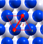
Figure 5: Geometry of the smallest three-atom clusters in the monolayer of 3$d$-atoms on $M(111)$ surface ($M$= Au, Ir): $M$-centered triangle $\Delta_{1}$ and hole-centered triangle $\Delta_{2}$.

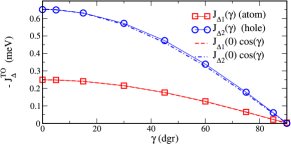
(a)
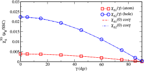
 (b)

Figure 6: (a) Three-spin chiral exchange interaction parameters $-J_{\Delta}(\gamma)$ (’minus’ is used to stress the relation between $J_{\Delta}$ and $\chi^{\rm{TO}}_{\Delta}$), and (bc) topological orbital susceptibility (TOS, for SOC = 0), calculated for Fe on Ir (111), as a function of the angle between the magnetization and normal $\hat{n}$ to the surface, for the smallest triangles $\Delta_{1}$ and $\Delta_{2}$. The dashed lines represent $J_{\Delta}(0)\,\cos(\gamma)$ (a) and $\chi^{\rm{TO}}_{\Delta}(0)\,\cos(\gamma)$ (b), respectively. All data are taken from Ref. Mankovsky et al., 2021.

The role of the SOC for the three-site 4-spin DMI-like interaction, ${\cal D}^{z}_{ijik}$, and the three-spin chiral interaction, $J_{\Delta}$ is shown in Fig. 7. These quantities are calculated for 1ML Fe on Au (111), for the two smallest triangles $\Delta_{1}$ and $\Delta_{2}$ centered at an Au atom or a hole site, respectively (see Fig. 5). Here, setting the SOC scaling factor $\xi_{\rm{SOC}}=0$ implies a suppression of the SOC, while $\xi_{\rm{SOC}}=1$ corresponds to the fully relativistic case. Fig. 7 (a) shows the three-site 4-spin DMI-like interaction parameter, ${\cal D}^{z}_{ijik}(\xi_{\rm{SOC}})$ when the SOC scaling parameter $\xi_{\rm{SOC}}$ applied to all components in the system, shown by full symbols, and with the SOC scaling applied only to the Au substrate. One can see a dominating role of the SOC of substrate atoms for ${\cal D}^{z}_{ijik}$. Also in Fig. 7 (b), a nearly linear variation can be seen for $J_{\Delta}(\xi_{\rm{SOC}})$ when the SOC scaling parameter $\xi_{\rm{SOC}}$ is applied to all components in the system (full symbols). Similar to ${\cal D}^{z}_{ijik}$, this shows that the SOC is an ultimate prerequisite for a non-vanishing TCI $J_{\Delta}$. When scaling the SOC only for Au (open symbols), Fig. 7 (b) show only weak changes for the TCI parameters $J_{\Delta}(\xi_{\rm{SOC}})$, demonstrating a minor impact of the SOC of the substrate on these interactions, in contrast to the DMI-like interaction shown in Fig. 7 (a). One can see also that ${\cal D}^{z}_{ijik}$ is about two orders of magnitude smaller than $J_{\Delta}$ for this particular system.

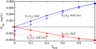
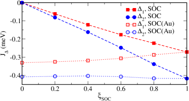
(a) (b)

Figure 7: (a) Three-site 4-spin DMI-like interaction, ${\cal D}^{z}_{ijkj}$ and (c) three-spin chiral exchange interaction (TCI) parameters $J_{\Delta}$ calculated for Fe on Au (111) on the basis of Eq. (75) as a function of SOC scaling parameter $\xi_{SOC}$ for the smallest triangles $\Delta_{1}$ and $\Delta_{2}$. In figure (b), full symbols represent the results obtained when scaling the SOC for all elements in the system, while open symbols show the results when scaling only the SOC for Au. All data are taken from Ref. Mankovsky et al., 2021.

The origin of the TCI parameters have been discussed in the literature suggesting a different interpretation of the corresponding terms derived also within the multiple-scattering theory Green function formalism Brinker et al. (2019); Grytsiuk et al. (2020); dos Santos Dias et al. (2021). However, the expression worked out in Ref. Grytsiuk et al., 2020 has obviously not been applied for calculations so far. As pointed out in Ref. Mankovsky et al., 2021, the different interpretation of this type of interactions can be explained by their different origin. In particular, one has to stress that the parameters in Refs. Mankovsky et al., 2021 and Grytsiuk et al., 2020 were derived in a different order of perturbation theory. On the other hand, the approach used for calculations of the multispin exchange parameters reported in Ref. Brinker et al., 2019; Grytsiuk et al., 2020; Lounis, 2020 is very similar to the one used in Refs. Mankovsky et al., 2020, 2021. The corresponding expressions have been worked out within the framework of multiple-scattering Green function formalism using the magnetic force theorem. In particular, the Lloyd formula has been used to express the energy change due to the perturbation $\Delta V$ leading to the expression

$$\Delta{\cal E} = -\frac{1}{\pi}\mbox{Im\, Tr\,}\int^{E_{F}}dE\,\sum_{p}\frac{1}{p}\mbox{Tr}\left[\underline{\underline{G}}(E)\,\Delta\underline{\underline{V}}\right]^{p}\,.$$ (77)

Using the off-site part of the GF in Eq. (35), as defined by Dederichs et al. Dederichs et al. (1992), Eq. (77) is transformed to the form

$$\Delta{\cal E} = -\frac{1}{\pi}\mbox{Im\, Tr\,}\int^{E_{F}}dE\,\sum_{p}\frac{1}{p}\mbox{Tr}\left[\underline{\underline{G}}^{\mbox{str}}(E)\,\underline{\underline{\Delta t}}(E)\right]^{p}\,.$$ (78)

By splitting the structural Green function ${\underline{G}}_{ij}^{\mbox{str}}$ into a spin-dependent ($\vec{\underline{B}}_{ij}^{\mbox{str}}$) and a spin-independent (${\underline{A}}_{ij}^{\mbox{str}}$) parts according to

$${\underline{G}}_{ij}^{\mbox{str}} = {\underline{A}}_{ij}^{\mbox{str}}\sigma_{0}+\vec{\underline{B}}_{ij}^{\mbox{str}}\cdot\vec{\sigma}$$ (79)

and expressing the change of the single-site scattering matrix

$$\underline{\Delta t}_{i}(E)=(\underline{t}^{\uparrow}_{i}(E)-\underline{t}^{\downarrow})\delta\hat{s}_{i}\times\vec{\sigma}\,,$$ (80)

by means of the rigid spin approximation, the different terms in Eq. (78) corresponding to different numbers $p$ give access to corresponding multispin terms, chiral and non-chiral, in the extended spin Hamiltonian. In particular, the isotropic six-spin interactions, that are responsible for the non-collinear magnetic structure of B20-MnGe according to Grytsiuk et al Grytsiuk et al. (2020), is given by the expression

$$\kappa^{6-spin}_{ijklmn} = \frac{1}{3\pi}\mbox{Im Tr}\int^{E_{F}}dE$$ (81)

$$\times A_{ij}t^{\sigma}_{j}A_{jk}t^{\sigma}_{k}A_{kl}t^{\sigma}_{l}A_{lm}t^{\sigma}_{m}A_{mn}t^{\sigma}_{n}A_{ni}t^{\sigma}_{i}\,.$$

A rather different point of view concerning the multispin extension of the spin Hamiltonian was adopted by Streib et al. Streib et al. (2021, 2022), who suggested to distinguish so-called local and global Hamiltonians. According to that classification, a global Hamiltonian implies to include in principle all possible spin configurations for the energy mapping in order to calculate exchange parameters that characterize in turn the energy of any spin configuration. On the other hand, a local Hamiltonian is ’designed to describe the energetics of spin configurations in the vicinity of the ground state or, more generally, in the vicinity of a predefined spin configuration’ Streib et al. (2021). This implies that taking the ground state as a reference state, it has to be determined first before the calculating the exchange parameters which are in principle applicable only for small spin tiltings around the reference state and can be used e.g. to investigate spin fluctuations around the ground state spin configuration. In Ref. Streib et al., 2021, the authors used a constraining field to stabilize the non-collinear magnetic configuration. This leads to the effective two-spin exchange interactions corresponding to a non-collinear magnetic spin configuration Streib et al. (2021, 2022). According to the authors, ’local spin Hamiltonians do not require any spin interactions beyond the bilinear order (for Heisenberg exchange as well as Dzyaloshinskii-Moriya interactions)’. On the other hand, they point out the limitations for these exchange interactions in the case of non-collinear system in the regime when the standard Heisenberg model is not validStreib et al. (2022), and multi-spin interactions get more important.

II Gilbert damping

Another parameter entering the Landau-Lifshitz-Gilbert (LLG) equation in Eq. (3) is the Gilbert damping parameter $\tilde{G}$ characterizing energy dissipation associated with the magnetization dynamics.

Theoretical investigations on the Gilbert damping parameter have been performed by various groups and accordingly the properties of GD is discussed in detail in the literature. Many of these investigations are performed assuming a certain dissipation mechanism, like Kambersky’s breathing Fermi surface (BFS) Kambersky (1970); Fähnle and Steiauf (2006), or more general torque-correlation models (TCM) Kambersky (1976); Gilmore et al. (2007) to be evaluated on the basis of electronic structure calculations. The earlier works in the field relied on the relaxation time parameter that represents scattering processes responsible for the energy dissipation. Only few computational schemes for Gilbert damping parameter account explicitly for disorder in the systems, which is responsible for the spin-flip scattering process. This issue was addressed in particular by Brataas et al. Brataas et al. (2008) who described the Gilbert damping mechanism by means of scattering theory. This development supplied the formal basis for the first parameter-free investigations on disordered alloys Starikov et al. (2010); Ebert et al. (2011b); Mankovsky et al. (2013).

A formalism for the calculation of the Gilbert damping parameter based on linear response theory has been reported in Ref. Mankovsky et al., 2013 and implemented using fully relativistic multiple scattering or Korringa-Kohn-Rostoker (KKR) formalism. Considering the FM state as a reference state of the system, the energy dissipation can be expressed in terms of the GD parameter by:

$$\dot{E}_{\rm mag}=\vec{H}_{\rm eff}\cdot\frac{d\vec{M}}{d\tau}=\frac{1}{\gamma^{2}}\dot{\vec{m}}[\tilde{G}(\vec{m})\dot{\vec{m}}]\,.$$ (82)

On the other hand, the energy dissipation in the electronic system is determined by the underlying Hamiltonian $\hat{H}(\tau)$ as follows $\dot{E}_{\rm dis}=\left\langle\frac{d\hat{H}}{d\tau}\right\rangle$. Assuming a small deviation of the magnetic moment from the equilibrium $\vec{u}(\tau)$, the normalized magnetization $\vec{m}(\tau)$ can be written in a linearized form $\vec{m}(\tau)=\vec{m}_{0}+\vec{u}(\tau)$, that in turn leads to the linearized time dependent electronic Hamiltonian $\hat{H}(\tau)$

$$\hat{H}=\hat{H}_{0}(\vec{m}_{0})+\sum_{\mu}\vec{u}_{\mu}\frac{\partial}{\partial\vec{u}_{\mu}}\hat{H}(\vec{m}_{0})\;.$$ (83)

As shown in Ref. Ebert et al., 2011b, the energy dissipation within the linear response formalism is given by:

$$\dot{\cal E}_{\rm dis} = -\pi\hbar\sum_{ij}\sum_{\mu\nu}\dot{u}_{\mu}\dot{u}_{\nu}\left\langle\psi_{i}\bigg{|}\frac{\partial\hat{H}}{\partial u_{\mu}}\bigg{|}\psi_{j}\right\rangle\left\langle\psi_{j}\bigg{|}\frac{\partial\hat{H}}{\partial u_{\nu}}\bigg{|}\psi_{i}\right\rangle$$ (84)

$$\;\;\;\;\;\;\;\;\;\;\;\;\;\;\;\;\;\;\times\delta(E_{F}-E_{i})\delta(E_{F}-E_{j})\;.$$

Identifying it with the corresponding phenomenological quantity in Eq. (82), $\dot{E}_{\rm mag}=\dot{\cal E}_{\rm dis}$ one obtains for the GD parameter $\alpha$ a Kubo-Greenwood-like expression:

$$\alpha_{\mu\nu} = -\frac{\hbar\gamma}{\pi M_{s}}\mbox{Trace}\left\langle\frac{\partial\hat{H}}{\partial u_{\mu}}\mbox{Im}\;G^{+}(E_{F})\frac{\partial\hat{H}}{\partial u_{\nu}}\mbox{Im}\;G^{+}(E_{F})\right\rangle_{c}\;,$$

where $\alpha=\tilde{G}/(\gamma M_{s})$, and $\langle...\rangle_{c}$ indicates a configurational average required in the presence of chemical or thermally induced disorder responsible for the dissipation processes. Within the multiple scattering formalism with the representation of the Green function given by Eq. (9), Eq. (LABEL:alpha2) leads to

$$\alpha_{\mu\mu}=\frac{g}{\pi\mu_{tot}}\sum_{n}\mbox{ Trace}\left\langle\underline{T}^{0\mu}\,\tilde{\underline{\tau}}^{0n}\,\underline{T}^{n\mu}\,\tilde{\underline{\tau}}^{n0}\right\rangle_{c}$$ (86)

with the g-factor $2(1+{\mu_{orb}}/{\mu_{spin}})$ in terms of the spin and orbital moments, $\mu_{spin}$ and $\mu_{orb}$, respectively, the total magnetic moment $\mu_{tot}=\mu_{spin}+\mu_{orb}$, and $\tilde{\tau}_{\Lambda\Lambda^{\prime}}^{0n}=\frac{1}{2i}(\tau_{\Lambda\Lambda^{\prime}}^{0n}-\tau_{\Lambda^{\prime}\Lambda}^{0n})$ and with the energy argument $E_{F}$ omitted. The matrix elements $\underline{T}^{n\mu}$ are identical to those occurring in the context of exchange coupling Ebert and Mankovsky (2009) and can be expressed in terms of the spin-dependent part $B$ of the electronic potential with matrix elements:

$$T_{\Lambda^{\prime}\Lambda}^{n\mu} = \int d^{3}r\;Z^{n\times}_{\Lambda^{\prime}}(\vec{r})\;\left[\beta\sigma_{\mu}B_{xc}(\vec{r})\right]Z^{n}_{\Lambda}(\vec{r})\;.$$ (87)

As is discussed in Ref. Mankovsky et al., 2013, for a system having chemical disorder, the configurational average is performed using the scattering path operators evaluated on the basis of the coherent potential approximation (CPA) alloy theory. In the case of thermally induced disorder, the alloy analogy model is used, which was discussed already above. When evaluating Eq. (86), the so-called vertex corrections have to be includedButler (1985) that accounts for the difference between the averages $\left\langle T_{\mu}\mbox{Im}G^{+}T_{\nu}\mbox{Im}G^{+}\right\rangle_{c}$ and $\left\langle T_{\mu}\mbox{Im}G^{+}\right\rangle_{c}\left\langle T_{\nu}\mbox{Im}G^{+}\right\rangle_{c}$. Within the Boltzmann formalism these corrections account for scattering-in processes.

The crucial role of these corrections is demonstrated Mankovsky et al. (2013) in Fig. 8 representing the Gilbert damping parameter for an Fe_1-xV_x disordered alloy as a function of the concentration $x$, calculated with and without vertex corrections. As one can see, neglect of the vertex corrections may lead to the nonphysical result $\alpha<0$. This wrong behavior does not occur when the vertex corrections are included, that obviously account for energy transfer processes connected with scattering-in processes.

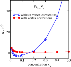
(a)

Figure 8: The Gilbert damping parameter for (a) bcc Fe_1-xV_x ($T=0$ K) as a function of V concentration. Full (open) symbols give results with (without) the vertex corrections. All data are taken from Ref. Mankovsky et al., 2013.

The impact of thermal vibrations onto the Gilbert damping can be taken into account within the alloy-analogy model (see above) by averaging over a discrete set of thermal atom displacements for a given temperature $T$. Fig. 9 represents the temperature dependent behavior of the Gilbert damping parameter $\alpha$ for bcc Fe with $1\%$ and $5\%$ of impurities of Os and Pt Ebert et al. (2011b); Mankovsky et al. (2013). One can see a strong impact of impurities on GD. In the case of $1\%$ of Pt in Fig. 9 (a), $\alpha$ decreases in the low-temperature regime much steeper upon increasing the temperature, indicating that the breathing Fermi surface mechanism dominates. When the concentration of the impurities increases up to $5\%$ (Fig. 9 (a)), the spin-flip scattering mechanism takes the leading role for the magnetization dissipation practically for the whole region of temperatures under consideration. The different behavior of GD for Fe with Os and Pt is a result of the different density of states (DOS) of the impurities at the Fermi energy (see Ref. Mankovsky et al., 2013 for a discussion).

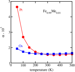
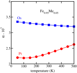
(a)  (b)

Figure 9: Gilbert damping parameter for bcc Fe_1-x$M_{x}$ with $M=$ Pt (circles) and $M=$ Os (squares) impurities as a function of temperature for 1% (a) and 5% (b) of the impurities. All data are taken from Ref. Mankovsky et al., 2013.

The role of the electron-phonon scattering for the ultrafast laser-induced demagnetization was investigated by Carva et al. Carva et al. (2013) based on the Elliott-Yafet theory of spin relaxation in metals, that puts the focus on spin-flip (SF) transitions upon the electron-phonon scattering. As the evaluation of the spin-dependent electron-phonon matrix elements entering the expression for the rate of the spin-flip transition is a demanding problem, various approximations are used for this. In particular, Carva et al. Carva et al. (2011, 2013) use the so-called Elliott approximation to evaluate a SF probability $P_{S}^{b}=\frac{\tau}{\tau_{sf}}$ with the spin lifetime $\tau_{sf}$ and a spin-diagonal lifetime $\tau$:

$$P_{S}^{b} = \frac{\tau}{\tau_{sf}}=4\langle b^{2}\rangle$$ (88)

with the Fermi-surface averaged spin mixing of Bloch wave eigenstates

$$\langle b^{2}\rangle = \sum_{\sigma,n}\int d^{3}k|b^{\sigma}_{\vec{k}n}|\delta(E^{\sigma}_{\vec{k}n}-E_{F})\,.$$ (89)

In the case of a non-collinear magnetic structure, the description of the Gilbert damping can be extended by adding higher-order non-local contributions. The role of non-local damping contributions has been investigated by calculating the precession damping $\alpha(\vec{q})$ for magnons in FM metals, characterized by a wave vector $\vec{q}$. Following the same idea, Thonig et al. Thonig et al. (2018) used a torque-torque correlation model based on a tight binding approach, and calculated the Gilbert damping for the itinerant-electron ferromagnets Fe, Co and Ni, both in the reciprocal, $\alpha(\vec{q})$, and real $\alpha_{ij}$ space representations. The important role of non-local contributions to the GD for spin dynamics has been demonstrated using atomistic magnetization dynamics simulations.

A formalism for calculating the non-local contributions to the GD has been recently worked out within the KKR Green function formalism Mankovsky et al. (2018). Using linear response theory for weakly-noncollinear magnetic systems it gives access to the GD parameters represented as a function of a wave vector $\vec{q}$. Using the definition for the spin susceptibility tensor $\chi_{\alpha\beta}(\vec{q},\omega)$, the Fourier transformation of the real-space Gilbert damping can be represented by the expression Qian and Vignale (2002); Hankiewicz et al. (2007)

$$\alpha_{\alpha\beta}(\vec{q}) = \frac{\gamma}{M_{0}V}\lim_{\omega\to 0}\frac{\partial\Im[\chi^{-1}]_{\alpha\beta}(\vec{q},\omega)}{\partial\omega}\;.$$ (90)

Here $\gamma=g\mu_{B}$ is the gyromagnetic ratio, $M_{0}=\mu_{tot}\mu_{B}/V$ is the equilibrium magnetization and $V$ is the volume of the system. As is shown in Ref. Mankovsky et al., 2018, this expression can be transformed to the form which allows an expansion of GD in powers of wave vector $\vec{q}$:

$${\underline{\alpha}}(\vec{q}) = {\underline{\alpha}}+\sum_{\mu}\underline{\alpha}^{\mu}q_{\mu}+\frac{1}{2}\sum_{\mu\nu}\underline{\alpha}^{\mu\nu}q_{\mu}q_{\nu}+...\,.$$ (91)

with the following expansion coefficients:

$$\alpha^{0\pm\pm}_{\alpha\alpha} = \frac{g}{\pi\mu_{tot}}\frac{1}{\Omega_{BZ}}{\mbox{Tr}}\int d^{3}k\bigg{\langle}\underline{T}_{\beta}\underline{\tau}(\vec{k},E_{F}^{\pm})\underline{T}_{\beta}\underline{\tau}(\vec{k},E_{F}^{\pm})\bigg{\rangle}_{c}$$

$$\alpha_{\alpha\alpha}^{\mu\pm\pm} = \frac{g}{\pi\mu_{tot}}\frac{1}{\Omega_{BZ}}{\mbox{Tr}}\int d^{3}k\bigg{\langle}\underline{T}^{\beta}\frac{\partial\underline{\tau}(\vec{k},E_{F}^{\pm})}{\partial k_{\mu}}\underline{T}^{\beta}\underline{\tau}(\vec{k},E_{F}^{\pm})\bigg{\rangle}_{c}$$

$$\alpha_{\alpha\alpha}^{\mu\nu\pm\pm} = -\frac{g}{2\pi\mu_{tot}}\frac{1}{\Omega_{BZ}}$$ (92)

$$\times{\mbox{Tr}\int d^{3}k}\bigg{\langle}\underline{T}^{\beta}\frac{\partial\underline{\tau}(\vec{k},E_{F}^{\pm})}{\partial k_{\mu}}\underline{T}^{\beta}\frac{\partial\underline{\tau}(\vec{k},E_{F}^{\pm})}{\partial k_{\nu}}\bigg{\rangle}_{c}\;.$$

For the prototype multilayer system (Cu/Fe_1-xCo_x/Pt)_n the calculated zero-order (uniform) GD parameter $\alpha_{xx}$ and the corresponding first-order (chiral) $\alpha^{x}_{xx}$ correction term for $\vec{q}\,\|\hat{x}$ are plotted in Fig. 10 top and bottom, respectively, as a function of the Co concentration $x$.

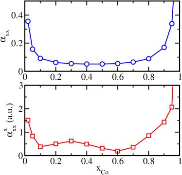
Figure 10: The Gilbert damping parameters $\alpha_{xx}$ (top) and $\alpha^{x}_{xx}$ (bottom) calculated for the model multilayer system (Cu/Fe_1-xCo_x/Pt)_n using first and second expressions in Eq. (II), respectively. All data are taken from Ref. Mankovsky et al., 2018.

Both terms, $\alpha_{xx}$ and $\alpha^{x}_{xx}$, increase approaching the pure limits w.r.t. the Fe_1-xCo_x alloy subsystem. As is pointed out in Ref. Mankovsky et al., 2018, this increase is associated with the dominating so-called breathing Fermi-surface damping mechanism due to the modification of the Fermi surface (FS) induced by the SOC, which follows the magnetization direction that slowly varies with time. As $\underline{\alpha}$ is caused for a ferromagnet exclusively by the SOC one can expect that it vanishes for vanishing SOC. This was indeed demonstrated before Mankovsky et al. (2013). The same holds also for $\underline{\alpha}^{x}$ that is caused by SOC as well.

Alternatively, a real-space extension for classical Gilbert damping tensor was proposed recently by Brinker et al. Brinker et al. (2022), by introducing two-site Gilbert damping tensor $\underline{\cal G}_{ij}$ entering the site-resolved LLG equation

$$\frac{1}{\gamma}\frac{d\vec{M}_{i}}{d\tau} = -\gamma\vec{M}_{i}\times\bigg{(}\vec{H}_{i,\rm eff}+\sum_{j}\left[\underline{\cal G}_{ij}(\vec{M})\cdot\frac{d\vec{M}_{i}}{d\tau}\right]\bigg{)}\;,$$ (93)

which is related to the inverse dynamical susceptibility $\underline{\chi}_{ij}$ via the expression

$$\frac{d}{d\omega}\mbox{Im}[\underline{\chi}]^{\alpha\beta}_{ij} = \delta_{ij}\bigg{(}\frac{1}{\gamma M_{i}}\epsilon_{\alpha\beta\gamma}\bigg{)}+\bigg{(}{\cal R}_{i}\underline{\cal G}_{ij}{\cal R}_{j}^{T}\bigg{)}_{\alpha\beta}\;,$$ (94)

where ${\cal R}_{i}$ and ${\cal R}_{j}$ are the rotation matrices to go from the global to the local frames of reference for atoms $i$ and $j$, respectively, assuming a non-collinear magnetic ground state in the system. Thus, an expression for the GD can be directly obtained using the adiabatic approximation for the slow spin-dynamics processes. This justifies the approximation $([\underline{\chi}]^{-1}(\omega))_{\omega}^{\prime}\approx([\underline{\chi}_{0}]^{-1}(\omega))_{\omega}^{\prime}$, with the un-enhanced dynamical susceptibility given in terms of electronic Green function $G_{ij}$

$$\chi^{\alpha\beta}_{ij}(\omega+i\eta) = -\frac{1}{\pi}\mbox{Tr}\int^{E_{F}}dE$$ (95)

$$\bigg{[}\sigma^{\alpha}{G}_{ij}(E+\omega+i\eta)\sigma^{\beta}\mbox{Im}{G}_{ij}(E)$$

$$+\sigma^{\alpha}{G}_{ij}(E)\sigma^{\beta}\mbox{Im}{G}_{ij}(E-\omega-i\eta)\bigg{]}\,,$$

with the Green function $G(E\pm i\eta)=(E-{\cal H}\pm i\eta)^{-1}$ corresponding to the Hamiltonian $\cal{H}$.

Moreover, this approach allows a multisite expansion of the GD accounting for higher-order non-local contributions for non-collinear structures Brinker et al. (2022). For this purpose, the Hamiltonian $\cal{H}$ is split into the on-site contribution $\cal{H}_{0}$ and the intersite hopping term $t_{ij}$, which is spin dependent in the general case. The GF can then be expanded in a perturbative way using the Dyson equation

$${G}_{ij} = {G}_{i}^{0}\delta_{ij}+{G}_{i}^{0}t_{ij}{G}_{j}^{0}+{G}_{i}^{0}t_{ik}{G}_{k}^{0}t_{kj}{G}_{j}^{0}+...\,.$$ (96)

As a result, the authors generalize the LLG equation by splitting the Gilbert damping tensor in terms proportional to scalar, anisotropic, vector-chiral and scalar-chiral products of the magnetic moments, i.e. terms like $\hat{e}_{i}\cdot\hat{e}_{j}$, $(\hat{n}_{ij}\cdot\hat{e}_{i})(\hat{n}_{ij}\cdot\hat{e}_{j})$, $\hat{n}_{ij}\cdot(\hat{e}_{i}\times\hat{e}_{j})$, etc.

It should be stressed that the Gilbert damping parameter accounts for the energy transfer connected with the magnetization dynamics but gives no information on the angular momentum transfer that plays an important role e.g. for ultrafast demagnetization processes. The formal basis to account simultaneously for the spin and lattice degrees of freedom was considered recently by Aßmann and Nowak Aßmann and Nowak (2019) and Hellsvik et al. Hellsvik et al. (2019). Hellsvik et al. Hellsvik et al. (2019); Sadhukhan et al. (2022) report on an approach solving simultaneously the equations for spin and lattice dynamics, accounting for spin-lattice interactions in the Hamiltonian, calculated on a first-principles level. These interactions appear as a correction to the exchange coupling parameters due to atomic displacements. As a result, this leads to the three-body spin-lattice coupling parameters $\Gamma_{ijk}^{\alpha\beta\mu}=\frac{\partial J^{\alpha\beta}_{ij}}{\partial u^{\mu}_{k}}$ and four-body parameters $\Lambda_{ijkl}^{\alpha\beta\mu\nu}=\frac{\partial J^{\alpha\beta}_{ij}}{\partial u^{\mu}_{k}\partial u^{\nu}_{l}}$ represented by rank 3 and rank 4 tensors, respectively, entering the spin-lattice Hamiltonian

$${\cal H}_{sl} = -\frac{1}{2}\sum_{i,j,k,\alpha\beta,\mu}\Gamma_{ijk}^{\alpha\beta\mu}e_{i}^{\alpha}e_{j}^{\beta}u^{\mu}_{k}$$ (97)

$$-\frac{1}{4}\sum_{i,j,k,l,\alpha\beta,\mu,\nu}\Lambda_{ijkl}^{\alpha\beta\mu\nu}e_{i}^{\alpha}e_{j}^{\beta}u^{\mu}_{k}u^{\nu}_{l}\;.$$

The parameters $\Gamma_{ijk}^{\alpha\beta\mu}$ in Ref. Hellsvik et al., 2019 are calculated using a finite difference method, using the exchange coupling parameters $\underline{J}_{ij}$ for the system without displacements ($\underline{J}^{0}_{ij}$) and with a displaced atom $k$ ($\underline{J}^{\Delta}_{ij}(\vec{u}_{k})$), used to estimate the coefficient $\Gamma_{ijk}^{\alpha\beta\mu}\approx\frac{(\underline{J}^{\Delta}_{ij}(\vec{u}_{k})-\underline{J}^{0}_{ij})}{u_{\mu}}$.

Alternatively, to describe the coupling of spin and spatial degrees of freedom the present authors (see Ref. Mankovsky et al., 2022) adopt an atomistic approach and start with the expansion of a phenomenological spin-lattice Hamiltonian

$${\cal H}_{sl} = -\sum_{i,j,\alpha,\beta}\sum_{k,\mu}J_{ij,k}^{\alpha\beta,\mu}e_{i}^{\alpha}e_{j}^{\beta}u^{\mu}_{k}$$ (98)

$$\qquad\qquad\quad-\sum_{i,j}\sum_{k,l}J_{ij,kl}^{\alpha\beta,\mu\nu}e_{i}^{\alpha}e_{j}^{\beta}u^{\mu}_{k}u^{\nu}_{l}\;,$$

that can be seen as a lattice extension of a Heisenberg model. Accordingly, the spin and lattice degrees of freedom are represented by the orientation vectors $\hat{e}_{i}$ of the magnetic moments $\vec{m}_{i}$ and displacement vectors $\vec{u}_{i}$ for each atomic site $i$. The spin-lattice Hamiltonian in Eq. (98) is restricted to three and four-site terms. As relativistic effects are taken into account, the SLC is described in tensorial form with $J_{ij,k}^{\alpha\beta,\mu}$ and $J_{ij,kl}^{\alpha\beta,\mu\nu}$ represented by rank 3 and rank 4 tensors, similar to those discussed by Hellsvik et al. Hellsvik et al. (2019).

The same strategy as for the exchange coupling parameters $J_{ij}$ Liechtenstein et al. (1987) or $J_{ij}^{\alpha\beta}$ Udvardi et al. (2003); Ebert and Mankovsky (2009), is used to map the free energy landscape ${\cal F}(\{\hat{e}_{i}\},\{\vec{u}_{i}\})$ accounting for its dependence on the spin configuration $\{\hat{e}_{i}\}$ as well as atomic displacements $\{\vec{u}_{i}\}$, making use of the magnetic force theorem and the Lloyd formula to evaluate integrated DOS $\Delta N(E)$. With this, the free energy change due to any perturbation in the system is given by Eq. (25).

Using as a reference the ferromagnetically ordered state of the system with a non-distorted lattice, and the perturbed state characterized by finite spin tiltings $\delta\hat{e}_{i}$ and finite atomic displacements $\vec{u}_{i}$ at site $i$, one can write the corresponding changes of the inverse $t$-matrix as $\Delta^{s}_{\mu}\underline{m}_{i}=\underline{m}_{i}(\delta\hat{e}_{i}^{\mu})-\underline{m}^{0}_{i}$ and $\Delta_{\nu}^{u}\underline{m}_{i}=\underline{m}_{i}({u}_{i}^{\nu})-\underline{m}^{0}_{i}$. This allows to replace the integrand in Eq. (11) by

$$\mbox{ln}\,\underline{\underline{\tau}}-\mbox{ln}\,\underline{\underline{\tau}}^{0} = -\ln\Big{(}1+\underline{\underline{\tau}}\,[\Delta^{s}_{\mu}\underline{\underline{m}}_{i}+\Delta_{\nu}^{u}\underline{\underline{m}}_{j}+...]\Big{)}\;,$$ (99)

where all site-dependent changes in the spin configuration $\{\hat{e}_{i}\}$ and atomic positions $\{\vec{u}_{i}\}$ are accounted for in a one-to-one manner by the various terms on the right hand side. Due to the use of the magnetic force theorem these blocks may be written in terms of the spin tiltings $\delta\hat{e}_{i}^{\mu}$ and atomic displacements of the atoms ${u}_{i}^{\nu}$ together with the corresponding auxiliary matrices $\underline{T}^{\mu}_{i}$ and ${\cal U}_{i}^{\nu}$, respectively, as

$$\Delta^{s}_{\mu}{\underline{m}}_{i} = \delta\hat{e}^{\mu}_{i}\,\underline{T}^{\mu}_{i}\,,$$ (100)

$$\Delta^{u}_{\nu}\underline{m}_{i} = u^{\nu}_{i}\underline{\cal U}_{i}^{\nu}\,.$$ (101)

Inserting these expressions into Eq. (99) and the result in turn into Eq. (25) allows us to calculate the parameters of the spin-lattice Hamiltonian as the derivatives of the free energy with respect to tilting angles and displacements. This way one gets for example for the three-site term:

$${\cal J}^{\alpha\beta,\mu}_{ij,k} = \frac{\partial^{3}{\cal F}}{\partial e^{\alpha}_{i}\,\partial e^{\beta}_{j}\,\partial u^{\mu}_{k}}=\frac{1}{2\pi}\mbox{Im\, Tr\,}\int^{E_{F}}dE\,\,$$ (102)

$$\times \Big{[}\underline{T}^{\alpha}_{i}\,\underline{\tau}_{ij}\underline{T}^{\beta}_{j}\,\underline{\tau}_{jk}\underline{\cal U}^{\mu}_{k}\,\underline{\tau}_{ki}+\underline{T}^{\alpha}_{i}\,\underline{\tau}_{ik}\underline{\cal U}^{\mu}_{k}\,\underline{\tau}_{kj}\underline{T}^{\beta}_{j}\,\underline{\tau}_{ji}\Big{]}\;\;$$

and for the four-site term:

$${\cal J}^{\alpha\beta,\mu\nu}_{ij,kl} = \frac{\partial^{4}{\cal F}}{\partial e^{\alpha}_{i}\,\partial e^{\beta}_{j}\,\partial u^{\mu}_{k}\partial u^{\nu}_{l}}=\frac{1}{4\pi}\mbox{Im\, Tr\,}\int^{E_{F}}dE\,\,$$ (103)

$$\times\Bigg{[}\underline{\cal U}^{\mu}_{k}\,\underline{\tau}_{ki}\,\underline{T}^{\alpha}_{i}\,\underline{\tau}_{ij}\,\underline{T}^{\beta}_{j}\,\,\underline{\tau}_{jl}\,\underline{\cal U}^{\nu}_{l}\,\underline{\tau}_{lk}\,$$

$$+\underline{T}^{\alpha}_{i}\,\underline{\tau}_{ik}\,\underline{\cal U}^{\mu}_{k}\,\underline{\tau}_{kj}\,\underline{T}^{\beta}_{j}\,\,\underline{\tau}_{jl}\,\underline{\cal U}^{\nu}_{l}\,\underline{\tau}_{li}\,$$

$$+\underline{\cal U}^{\mu}_{k}\,\underline{\tau}_{ki}\,\underline{T}^{\alpha}_{i}\,\underline{\tau}_{il}\,\underline{\cal U}^{\nu}_{l}\,\underline{\tau}_{lj}\,\underline{T}^{\beta}_{j}\,\,\underline{\tau}_{jk}\,$$

$$+\underline{T}^{\alpha}_{i}\,\underline{\tau}_{ik}\,\underline{\cal U}^{\mu}_{k}\,\underline{\tau}_{kl}\,\underline{\cal U}^{\nu}_{l}\,\underline{\tau}_{lj}\,\underline{T}^{\beta}_{j}\,\,\underline{\tau}_{ji}\Bigg{]}\,.$$

Fig. 11 shows corresponding results for the SLC parameters of bcc Fe, plotted as a function of the distance $r_{ij}$ for $i=k$ which implies that a displacement along the $x$ direction is applied for one of the interacting atoms. The absolute values of the DMI-like SLC parameters (DSLC) $|\vec{\cal D}|^{\mu=x}_{ij,k}$ (note that ${\cal D}^{z,\mu}_{ij,k}=\frac{1}{2}({\cal J}^{xy,\mu}_{ij,k}-{\cal J}^{yx,\mu}_{ij,k})$ ) show a rather slow decay with the distance $r_{ij}$. The isotropic SLC parameters ${\cal J}^{\mathrm{iso},\mu=x}_{ij,j}$, which have only a weak dependence on the SOC, are about one order of magnitude larger than the DSLC. All other SOC-driven parameters shown in Fig. 11, characterizing the displacement-induced contributions to MCA, are much smaller than the DSLC.

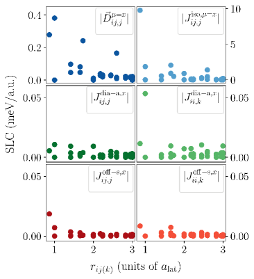
Figure 11: The absolute values of site-off-diagonal and site-diagonal SLC parameters: DMI $|\vec{\cal D}^{x}_{ij,j}|$ and isotropic SLC ${\cal J}^{\mathrm{iso},x}_{ij,j}$ (top), anti-symmetric diagonal components ${\cal J}^{\mathrm{dia-a},x}_{ij,j}$ and ${\cal J}^{\mathrm{dia-a},x}_{ii,k}$ (middle), and symmetric off-diagonal components ${\cal J}^{\mathrm{off-s},x}_{ij,j}$ and ${\cal J}^{\mathrm{off-s},x}_{ii,k}$ (bottom) for bcc Fe, as a function of the interatomic distance $r_{ij}$

III Summary

To summarize, we have considered a multi-level atomistic approach commonly used to simulate finite temperature and dynamical magnetic properties of solids, avoiding in particular time-consuming TD-SDFT calculations. The approach is based on a phenomenological parameterized spin Hamiltonian which allows to separate the spin and orbital degrees of freedom and that way to avoid the demanding treatment of complex spin-dependent many-body effects. As these parameters are fully determined by the electronic structure of a system, they can be deduced from the information provided by relativistic band structure calculations based on SDFT. We gave a short overview of the various methods to calculate these parameters entering for example the LLG equation. It is shown that the KKR Green function formalism is one of the most powerful band structure methods as it gives straightforward access to practically all parameters of the phenomenological models. It allows in particular to add in a very simple way further extensions to the model Hamiltonians, accounting for example for multi-site interaction terms. Another important issue are spin-lattice interactions, that couple the degrees of freedom of the spin and lattice subsystems. The key role of the SOC for the interaction parameters is pointed out as it gives not only rise to the MCA but also to the Gilbert damping as well as the anisotropy of the exchange coupling and spin-lattice interaction with many important physical phenomena connected to these.

References

- Engel and Dreizler (2011) E. Engel and R. M. Dreizler, Density Functional Theory – An advanced course (Springer, Berlin, 2011).
- Krieger et al. (2015) K. Krieger, J. K. Dewhurst, P. Elliott, S. Sharma, and E. K. U. Gross, Journal of Chemical Theory and Computation 11, 4870 (2015).
- Liechtenstein et al. (1984) A. I. Liechtenstein, M. I. Katsnelson, and V. A. Gubanov, J. Phys. F: Met. Phys. 14, L125 (1984).
- Liechtenstein et al. (1987) A. I. Liechtenstein, M. I. Katsnelson, V. P. Antropov, and V. A. Gubanov, J. Magn. Magn. Materials 67, 65 (1987).
- Udvardi et al. (2003) L. Udvardi, L. Szunyogh, K. Palotás, and P. Weinberger, Phys. Rev. B 68, 104436 (2003).
- Ebert and Mankovsky (2009) H. Ebert and S. Mankovsky, Phys. Rev. B 79, 045209 (2009).
- Heide et al. (2008) M. Heide, G. Bihlmayer, and S. Blügel, Phys. Rev. B 78, 140403 (2008).
- Heide et al. (2009) M. Heide, G. Bihlmayer, and S. Blugel, Physica B: Condensed Matter 404, 2678 (2009), proceedings of the Workshop - Current Trends and Novel Materials.
- Rusz et al. (2006) J. Rusz, L. Bergqvist, J. Kudrnovský, and I. Turek, Phys. Rev. B 73, 214412 (2006).
- Antropov et al. (1996) V. P. Antropov, M. I. Katsnelson, B. N. Harmon, M. van Schilfgaarde, and D. Kusnezov, Phys. Rev. B 54, 1019 (1996).
- Eriksson et al. (2022) O. Eriksson, A. Bergman, L. Bergqvist, and J. Hellsvik, Atomistic Spin Dynamics: Foundations and Applications. (Oxford University Press, 2022).
- Bornemann et al. (2012) S. Bornemann, J. Minár, J. Braun, D. Ködderitzsch, and H. Ebert, Solid State Commun. 152, 85 (2012).
- Blügel (1999) S. Blügel, in 30. Ferienkurs des Instituts für Festkörperforschung 1999 ”Magnetische Schichtsysteme”, edited by Institut für Festkörperforschung (Forschungszentrum Jülich GmbH, Jülich, 1999) p. C1.1.
- Razee et al. (1997) S. S. A. Razee, J. B. Staunton, and F. J. Pinski, Phys. Rev. B 56, 8082 (1997).
- Rose (1961) M. E. Rose, Relativistic Electron Theory (Wiley, New York, 1961).
- H. Ebert et al. (2020) H. Ebert et al., The Munich SPR-KKR package, version 8.5, https://www.ebert.cup.uni-muenchen.de/en/software-en/13-sprkkr (2020).
- Ebert et al. (2011a) H. Ebert, D. Ködderitzsch, and J. Minár, Rep. Prog. Phys. 74, 096501 (2011a).
- Ebert et al. (2016) H. Ebert, J. Braun, D. Ködderitzsch, and S. Mankovsky, Phys. Rev. B 93, 075145 (2016).
- Staunton et al. (2006) J. B. Staunton, L. Szunyogh, A. Buruzs, B. L. Gyorffy, S. Ostanin, and L. Udvardi, Phys. Rev. B 74, 144411 (2006).
- Gyorffy et al. (1985) B. L. Gyorffy, A. J. Pindor, J. Staunton, G. M. Stocks, and H. Winter, J. Phys. F: Met. Phys. 15, 1337 (1985).
- Soven (1967) P. Soven, Phys. Rev. 156, 809 (1967).
- Staunton et al. (2000) J. B. Staunton, J. Poulter, B. Ginatempo, E. Bruno, and D. D. Johnson, Phys. Rev. B 62, 1075 (2000).
- Faulkner and Stocks (1980) J. S. Faulkner and G. M. Stocks, Phys. Rev. B 21, 3222 (1980).
- Staunton et al. (2004) J. B. Staunton, S. Ostanin, S. S. A. Razee, B. L. Gyorffy, L. Szunyogh, B. Ginatempo, and E. Bruno, Phys. Rev. Lett. 93, 257204 (2004).
- Szilva et al. (2022) A. Szilva, Y. Kvashnin, E. A. Stepanov, L. Nordström, O. Eriksson, A. I. Lichtenstein, and M. I. Katsnelson, arXiv:2206.02415 (2022), 10.48550/ARXIV.2206.02415.
- Uhl et al. (1994) M. Uhl, L. M. Sandratskii, and J. Kübler, Phys. Rev. B 50, 291 (1994).
- Halilov et al. (1998) S. V. Halilov, H. Eschrig, A. Y. Perlov, and P. M. Oppeneer, Phys. Rev. B 58, 293 (1998).
- Sandratskii and Bruno (2002) L. M. Sandratskii and P. Bruno, Phys. Rev. B 66, 134435 (2002).
- Pajda et al. (2000) M. Pajda, J. Kudrnovský, I. Turek, V. Drchal, and P. Bruno, Phys. Rev. Lett. 85, 5424 (2000).
- Solovyev (2021) I. V. Solovyev, Phys. Rev. B 103, 104428 (2021).
- Grotheer et al. (2001) O. Grotheer, C. Ederer, and M. Fähnle, Phys. Rev. B 63, 100401 (2001).
- Antropov (2003) V. Antropov, Journal of Magnetism and Magnetic Materials 262, L192 (2003).
- Bruno (2003) P. Bruno, Phys. Rev. Lett. 90, 087205 (2003).
- Dederichs et al. (1992) P. H. Dederichs, B. Drittler, and R. Zeller, Mat. Res. Soc. Symp. Proc. 253, 185 (1992).
- Weinberger (1990) P. Weinberger, Electron Scattering Theory for Ordered and Disordered Matter (Oxford University Press, Oxford, 1990).
- Mankovsky et al. (2019) S. Mankovsky, S. Polesya, and H. Ebert, Phys. Rev. B 99 (2019), 10.1103/PhysRevB.99.104427.
- Mankovsky et al. (2020) S. Mankovsky, S. Polesya, and H. Ebert, Phys. Rev. B 101, 174401 (2020).
- Ebert et al. (2011b) H. Ebert, S. Mankovsky, D. Ködderitzsch, and P. J. Kelly, Phys. Rev. Lett. 107, 066603 (2011b), http://arxiv.org/abs/1102.4551v1 .
- Mankovsky et al. (2013) S. Mankovsky, D. Ködderitzsch, G. Woltersdorf, and H. Ebert, Phys. Rev. B 87, 014430 (2013).
- Ebert et al. (2015) H. Ebert, S. Mankovsky, K. Chadova, S. Polesya, J. Minár, and D. Ködderitzsch, Phys. Rev. B 91, 165132 (2015).
- Papanikolaou et al. (1997) N. Papanikolaou, R. Zeller, P. H. Dederichs, and N. Stefanou, Phys. Rev. B 55, 4157 (1997).
- Lodder (1976) A. Lodder, J. Phys. F: Met. Phys. 6, 1885 (1976).
- Butler (1985) W. H. Butler, Phys. Rev. B 31, 3260 (1985).
- Harris and Owen (1963) E. A. Harris and J. Owen, Phys. Rev. Lett. 11, 9 (1963).
- Huang and Orbach (1964) N. L. Huang and R. Orbach, Phys. Rev. Lett. 12, 275 (1964).
- Allan and Betts (1967) G. A. T. Allan and D. D. Betts, Proceedings of the Physical Society 91, 341 (1967).
- Iwashita and Uryâ (1974) T. Iwashita and N. Uryâ, Journal of the Physical Society of Japan 36, 48 (1974), https://doi.org/10.1143/JPSJ.36.48 .
- Iwashita and Uryû (1976) T. Iwashita and N. Uryû, Phys. Rev. B 14, 3090 (1976).
- Aksamit (1980) J. Aksamit, Journal of Physics C: Solid State Physics 13, L871 (1980).
- Brown (1984) H. Brown, Journal of Magnetism and Magnetic Materials 43, L1 (1984).
- Ivanov et al. (2014) N. B. Ivanov, J. Ummethum, and J. Schnack, The European Physical Journal B 87, 226 (2014).
- Antal et al. (2008) A. Antal, B. Lazarovits, L. Udvardi, L. Szunyogh, B. Újfalussy, and P. Weinberger, Phys. Rev. B 77, 174429 (2008).
- Müller-Hartmann et al. (1997) E. Müller-Hartmann, U. Köbler, and L. Smardz, Journal of Magnetism and Magnetic Materials 173, 133 (1997).
- Greiter and Thomale (2009) M. Greiter and R. Thomale, Phys. Rev. Lett. 102, 207203 (2009).
- Greiter et al. (2014) M. Greiter, D. F. Schroeter, and R. Thomale, Phys. Rev. B 89, 165125 (2014).
- Fedorova et al. (2015) N. S. Fedorova, C. Ederer, N. A. Spaldin, and A. Scaramucci, Phys. Rev. B 91, 165122 (2015).
- Mendive-Tapia et al. (2021) E. Mendive-Tapia, M. dos Santos Dias, S. Grytsiuk, J. B. Staunton, S. Blügel, and S. Lounis, Phys. Rev. B 103, 024410 (2021).
- Gutzeit et al. (2021) M. Gutzeit, S. Haldar, S. Meyer, and S. Heinze, Phys. Rev. B 104, 024420 (2021).
- Hayami (2022) S. Hayami, Phys. Rev. B 105, 024413 (2022).
- Lászlóffy et al. (2019) A. Lászlóffy, L. Rózsa, K. Palotás, L. Udvardi, and L. Szunyogh, Phys. Rev. B 99, 184430 (2019).
- Paul et al. (2020) S. Paul, S. Haldar, S. von Malottki, and S. Heinze, Nature Communications 1, 475 (2020).
- Brinker et al. (2019) S. Brinker, M. dos Santos Dias, and S. Lounis, New Journal of Physics 21, 083015 (2019).
- Brinker et al. (2020) S. Brinker, M. dos Santos Dias, and S. Lounis, Phys. Rev. Research 2, 033240 (2020).
- Mankovsky and Ebert (2017) S. Mankovsky and H. Ebert, Phys. Rev. B 96, 104416 (2017).
- Solenov et al. (2012) D. Solenov, D. Mozyrsky, and I. Martin, Phys. Rev. Lett. 108, 096403 (2012).
- Okubo et al. (2012) T. Okubo, S. Chung, and H. Kawamura, Phys. Rev. Lett. 108, 017206 (2012).
- Batista et al. (2016) C. D. Batista, S.-Z. Lin, S. Hayami, and Y. Kamiya, Reports on Progress in Physics 79, 084504 (2016).
- Mankovsky et al. (2021) S. Mankovsky, S. Polesya, and H. Ebert, Phys. Rev. B 104, 054418 (2021).
- Grytsiuk et al. (2020) S. Grytsiuk, J.-P. Hanke, M. Hoffmann, J. Bouaziz, O. Gomonay, G. Bihlmayer, S. Lounis, Y. Mokrousov, and S. Blügel, Nature Communications 11, 511 (2020).
- dos Santos Dias et al. (2021) M. dos Santos Dias, S. Brinker, A. Lászlóffy, B. Nyári, S. Blügel, L. Szunyogh, and S. Lounis, Phys. Rev. B 103, L140408 (2021).
- Lounis (2020) S. Lounis, New Journal of Physics 22, 103003 (2020).
- Streib et al. (2021) S. Streib, A. Szilva, V. Borisov, M. Pereiro, A. Bergman, E. Sjöqvist, A. Delin, M. I. Katsnelson, O. Eriksson, and D. Thonig, Phys. Rev. B 103, 224413 (2021).
- Streib et al. (2022) S. Streib, R. Cardias, M. Pereiro, A. Bergman, E. Sjöqvist, C. Barreteau, A. Delin, O. Eriksson, and D. Thonig, “Adiabatic spin dynamics and effective exchange interactions from constrained tight-binding electronic structure theory: beyond the heisenberg regime,” (2022).
- Kambersky (1970) V. Kambersky, Can. J. Phys. 48, 2906 (1970).
- Fähnle and Steiauf (2006) M. Fähnle and D. Steiauf, Phys. Rev. B 73, 184427 (2006).
- Kambersky (1976) V. Kambersky, Czech. J. Phys. 26, 1366 (1976).
- Gilmore et al. (2007) K. Gilmore, Y. U. Idzerda, and M. D. Stiles, Phys. Rev. Lett. 99, 027204 (2007).
- Brataas et al. (2008) A. Brataas, Y. Tserkovnyak, and G. E. W. Bauer, Phys. Rev. Lett. 101, 037207 (2008).
- Starikov et al. (2010) A. A. Starikov, P. J. Kelly, A. Brataas, Y. Tserkovnyak, and G. E. W. Bauer, Phys. Rev. Lett. 105, 236601 (2010).
- Carva et al. (2013) K. Carva, M. Battiato, D. Legut, and P. M. Oppeneer, Phys. Rev. B 87, 184425 (2013).
- Carva et al. (2011) K. Carva, M. Battiato, and P. M. Oppeneer, Phys. Rev. Lett. 107, 207201 (2011).
- Thonig et al. (2018) D. Thonig, Y. Kvashnin, O. Eriksson, and M. Pereiro, Phys. Rev. Materials 2, 013801 (2018).
- Mankovsky et al. (2018) S. Mankovsky, S. Wimmer, and H. Ebert, Phys. Rev. B 98, 104406 (2018).
- Qian and Vignale (2002) Z. Qian and G. Vignale, Phys. Rev. Lett. 88, 056404 (2002).
- Hankiewicz et al. (2007) E. M. Hankiewicz, G. Vignale, and Y. Tserkovnyak, Phys. Rev. B 75, 174434 (2007).
- Brinker et al. (2022) S. Brinker, M. dos Santos Dias, and S. Lounis, Journal of Physics: Condensed Matter 34, 285802 (2022).
- Aßmann and Nowak (2019) M. Aßmann and U. Nowak, Journal of Magnetism and Magnetic Materials 469, 217 (2019).
- Hellsvik et al. (2019) J. Hellsvik, D. Thonig, K. Modin, D. Iuşan, A. Bergman, O. Eriksson, L. Bergqvist, and A. Delin, Phys. Rev. B 99, 104302 (2019).
- Sadhukhan et al. (2022) B. Sadhukhan, A. Bergman, Y. O. Kvashnin, J. Hellsvik, and A. Delin, Phys. Rev. B 105, 104418 (2022).
- Mankovsky et al. (2022) S. Mankovsky, S. Polesya, H. Lange, M. Weißenhofer, U. Nowak, and H. Ebert, arXiv:2203.16144v1 (2022), 10.48550/ARXIV.2203.16144.