Newton Cradle Spectra

Abstract

We present broadly applicable nonperturbative results on the behavior of eigenvalues and eigenvectors under the addition of self-adjoint operators and under the multiplication of unitary operators, in finite-dimensional Hilbert spaces. To this end, we decompose these operations into elementary 1-parameter processes in which the eigenvalues move similarly to the spheres in Newton’s cradle. As special cases, we recover level repulsion and Cauchy interlacing. We discuss two examples of applications. Applied to adiabatic quantum computing, we obtain new tools to relate algorithmic complexity to computational slowdown through gap narrowing. Applied to information theory, we obtain a generalization of Shannon sampling theory, the theory that establishes the equivalence of continuous and discrete representations of information. The new generalization of Shannon sampling applies to signals of varying information density and finite length.

The behavior of eigenvalues and eigenvectors plays important roles throughout science and engineering [1, 2, 3]. Of particular interest is, for example, their behavior under the addition of Hermitian operators, such as Hamiltonians, and under the multiplication of unitaries, such as time evolution operators. In the literature, this problem is often investigated perturbatively. Nonperturbative results, such as level repulsion [4, 5, 6] and Cauchy interlacing [7, 8], are particularly valuable but few in number [9]. Here, we present new broadly applicable nonperturbative results on the behavior of the spectra and eigenvectors of Hermitian and unitary operators in finite dimensions.

Addition of Hermitian operators. Let us consider an arbitrary Hermitian operator $S$ with nondegenerate spectrum, acting on an $N$-dimensional Hilbert space $\cal{H}$. We ask how the eigenvalues change when adding to $S$ an arbitrary Hermitian operator $R$. To this end, by the spectral theorem, we write $R$ as a weighted sum of rank 1 projectors: $R=\sum_{j=1}^{N}\mu^{(j)}|v^{(j)}\rangle\langle v^{(j)}|$. Since the sum $S+R$ can be obtained by successively adding these weighted projectors to $S$, we can focus on how the spectrum of $S$ changes under the addition of a single weighted projector:

$$S(\mu):=S+\mu|v\rangle\langle v|$$ (1)

Here, $|v\rangle$ is an arbitrary fixed normalized vector and we let the weight $\mu$ range from $-\infty$ to $+\infty$. We denote the eigenvalues and eigenvectors of $S$ by $\{s_{n}\},\{|s_{n}\rangle\}$ with the ordering $s_{1}<s_{2}<\ldots<s_{N}$. We denote the eigenvalues and eigenvectors of $S(\mu)$ by $\{s_{n}(\mu)\},\{|s_{n}(\mu)\rangle\}$ and we have $s_{n}(0)=s_{n},|s_{n}(0)\rangle=|s_{n}\rangle$. The ordering of the $s_{n}(\mu)$ is inherited from the ordering of the $s_{n}$, taking into account possible level crossings. The phases of the $|s_{n}(\mu)\rangle$ are left arbitrary for now.

First, the trivial special cases. If $|v\rangle$ is chosen so that $\langle s_{m}|v\rangle=0$ for some $m$, then the eigenspaces of $S$ spanned by the $|s_{m}\rangle$ remain unaffected, i.e., their eigenvalues and eigenvectors do not change with $\mu$: $s_{m}(\mu)=s_{m},|s_{m}(\mu)\rangle=|s_{m}\rangle~{}\forall\mu\in\mathbb{R}$. If we choose $|v\rangle$ to be an eigenvector, $|v\rangle:=|s_{r}\rangle$, then $\langle s_{m}|v\rangle=0~{}~{}\forall m\neq r$ and all eigenvectors and eigenvalues are frozen except that $s_{r}(\mu)=s_{r}+\mu,|s_{r}(\mu)\rangle=|s_{r}\rangle~{}\forall\mu\in\mathbb{R}$.
Newton cradle for Hermitian operators. We now consider the generic case in which $|v\rangle$ is not orthogonal to any eigenvectors of $S$. For this case, we can show that, as $\mu$ runs from $-\infty$ to $+\infty$, all $s_{n}(\mu)$ strictly monotonously move to the right, akin to Newton’s cradle: $s_{1}$ arrives from $-\infty$, the eigenvalues $s_{2}$ to $s_{N-1}$ each move a small distance to the right to take the next eigenvalue’s place and finally $s_{N}$ escapes to $+\infty$. As illustrated in Fig. 1, interlaced between the eigenvalues $s_{n}$, there exist numbers $s_{n}^{*}$ obeying $s_{n}<s_{n}^{*}<s_{n+1}$ for $n=1,\ldots,(N-1)$ so that, as we let $\mu$ run from $-\infty$ to $+\infty$, each eigenvalue $s_{n}(\mu)$ runs from $s_{n-1}^{*}$ to $s_{n}^{*}$, passing through $s_{n}$ when $\mu=0$. Here, $s_{0}^{*}:=-\infty$ and $s_{N}^{*}:=+\infty$.
Exact evolution of Hermitian Newton cradles. Due to the Newton cradle behavior of the eigenvalues, the full set of eigenvalues $\{s_{n}(\mu)\}$ for all $n=1\ldots N$ and all $\mu\in\mathbb{R}\cup\{+\infty\}$ cover the real line exactly once. For any $s\in\mathbb{R}$, there therefore exists a unique pair $(n,\mu)$ such that $|s\rangle:=|s_{n}(\mu)\rangle$ obeys $S(\mu)|s\rangle=s|s\rangle$. Defining $v_{n}:=\langle s_{n}|v\rangle$, we can show that for any $s\in\mathbb{R}$, the corresponding $\mu$ reads:

$$\mu(s)=\left(\sum_{n=1}^{N}\frac{\absolutevalue{v_{n}}^{2}}{s-s_{n}}\right)^{-1}$$ (2)

Eq. 2 can also be viewed as reexpressing the characteristic equation for $S(\mu)$. Eq. 2 implies that the values $s_{n}^{*}$ for $n=1\ldots(N-1)$ are the solutions to:

$$\sum_{m=1}^{N}\frac{\absolutevalue{v_{m}}^{2}}{s_{n}^{*}-s_{m}}=0$$ (3)

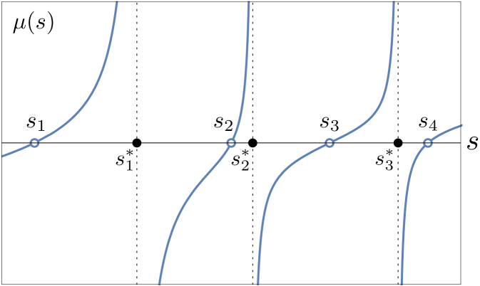
Figure 1: Plot of $\mu(s)$ using Eq. 2 for a random choice of Newton cradle of four eigenvalues. From bottom to top, the four curves show the evolution of the four eigenvalues $\{s_{n}(\mu)\}_{n=1}^{4}$ with increasing $\mu$. For $\mu=0$, the eigenvalues are $s_{1}$, $s_{2}$, $s_{3}$, $s_{4}$. As $\mu\rightarrow+\infty$, the eigenvalues tend to $s_{1}^{*}$, $s_{2}^{*}$, $s_{3}^{*}$ and $s_{4}^{*}=+\infty$ respectively.

Differentiating Eq. 2 yields:

$$\frac{d\mu(s)}{ds}=\left(\sum_{m=1}^{N}\frac{\absolutevalue{v_{m}}^{2}}{s-s_{m}}\right)^{-2}\sum_{r=1}^{N}\frac{\absolutevalue{v_{r}}^{2}}{\left(s-s_{r}\right)^{2}}$$ (4)

The inverse, $ds/d\mu$, is the velocity of the eigenvalues, $s$, with respect to $\mu$. The special case of the velocity $ds_{n}(\mu)/d\mu$ of an eigenvalue $s_{n}(\mu)$ at $\mu=0$ reads:

$$\frac{\differential s_{n}\left(\mu\right)}{\differential\mu}\evaluated{}_{\mu=0}=\absolutevalue{v_{n}}^{2}$$ (5)

These velocities are positive and stay positive for all finite $\mu$. This is because if a velocity $ds_{n}/d\mu$ vanished for a finite $\mu$, we would have $\langle s_{n}(\mu)|v\rangle=0$, hence this eigenvalue would be frozen for all $\mu$, in contradiction to the assumption that $\langle s_{n}|v\rangle\neq 0$. Further, since $\sum_{m=1}^{N}|v_{m}|^{2}=1$, the velocities sum to one. Since $d\Tr(S(\mu))/d\mu=\Tr(|v\rangle\langle v|)=1$ for all $\mu$, each Newton cradle conserves its total momentum in the sense that for all $\mu\in\mathbb{R}:~{}~{}\sum_{n=1}^{N}\frac{\differential s_{n}\left(\mu\right)}{\differential\mu}=1$.
Newton cradles for unitaries. An analogous result holds for unitaries. Let us consider an arbitrary fixed unitary $U$ acting on $\cal{H}$. Instead of adding a $1$-parameter family of projectors as we did above, we now multiplicatively act on $U$ from the left with a $U(1)$ group. The elements of this $U(1)$ act nontrivially on the dimension spanned by an arbitrary fixed vector, $|w\rangle$, and act as the identity on all other dimensions, i.e., we multiply $U$ from the left with the $U(1)$-family of unitaries $(\mathbb{1}+\left(e^{i\alpha}-1\right)\ket{w}\bra{w})$ for $\alpha\in[0,2\pi)$ to obtain a family of unitaries $U(\alpha)$:

$$U({\alpha}):=(\mathbb{1}+\left(e^{i\alpha}-1\right)\ket{w}\bra{w})\ U$$ (6)

Let us denote the eigenvalues of $U$ by $\{u_{n}\}$, ordered counterclockwise on the complex unit circle, starting from $1$. We denote the eigenvalues of $U(\alpha)$ by $u_{n}(\alpha)$, i.e., we have $u_{n}(0)=u_{n}$. We define $w_{n}:=\langle u_{n}|w\rangle$. Clearly, if $|w\rangle$ is chosen to obey $\langle u_{m}|w\rangle=0$ for some $m$ then the corresponding eigenvalues and eigenvectors are frozen, $u_{m}(\alpha)=u_{m},~{}|u_{m}(\alpha)\rangle=|u_{m}\rangle~{}\forall\alpha$. Excluding these trivial cases, we can show again a Newton cradle behavior: as $\alpha$ runs from $0$ to $2\pi$, each eigenvalue $u_{n}(\alpha)$ runs counterclockwise on the complex unit circle, reaching $u_{n+1}$ as $\alpha\rightarrow 2\pi$. Except, $u_{N}(\alpha)$ runs towards $u_{1}(\alpha)$.

Equivalence of unitary and Hermitian Newton cradles. We can show that the left multiplication of a unitary operator by a representation of the group $U(1)$ is equivalent to the addition of a weighted rank $1$ projector to a Hermitian operator. The equivalence is established by this Cayley transform:

$$U(\alpha)=(S(\mu)-i\mathbb{1})(S(\mu)+i\mathbb{1})^{-1}$$ (7)

$$S(\mu)=-i(U(\alpha)+\mathbb{1})(U(\alpha)-\mathbb{1})^{-1}$$ (8)

Therefore, $U(\alpha)$ and $S(\mu)$ possess the same eigenspaces and their eigenvalues are related by a Möbius transform: $u_{n}(\alpha)=(s_{n}(\mu)-i)/(s_{n}(\mu)+i)$. We can show that

$$\ket{v}=\frac{2}{\sqrt{\sum_{m=1}^{N}\absolutevalue{w_{m}}^{2}\left(s_{m}^{2}+1\right)}}\left(\mathbb{1}-U\right)^{-1}\ket{w}$$ (9)

and in coefficients:

$$v_{n} = \frac{1}{\sqrt{\sum_{m=1}^{N}\absolutevalue{w_{m}}^{2}\left(s_{m}^{2}+1\right)}}\frac{s_{n}+i}{i}w_{n}$$ (10)

$$w_{m} = \frac{1}{\sqrt{\sum_{k}\frac{\absolutevalue{v_{k}}^{2}}{s_{k}^{2}+1}}}\frac{i}{s_{m}+i}v_{m}$$ (11)

Further, $\mu$ and $\alpha$ are related by:

$$\alpha(\mu) = 2\arccot\left[\frac{\sum_{m}\absolutevalue{w_{m}}^{2}\left(s_{m}^{2}+1\right)}{\mu}+\sum_{k}\absolutevalue{w_{k}}^{2}s_{k}\right]$$

$$= 2\arccot\left[\left(\sum_{k}\frac{\absolutevalue{v_{k}}^{2}}{s_{k}^{2}+1}\right)^{-1}\left(\frac{1}{\mu}+\sum_{m}\frac{\absolutevalue{v_{m}}^{2}s_{m}}{s_{m}^{2}+1}\right)\right]$$

$$\mu\left(\alpha\right) = \frac{\sum_{m=1}^{N}\absolutevalue{w_{m}}^{2}\left(s_{m}^{2}+1\right)}{\cot\left(\frac{\alpha}{2}\right)-\sum_{k=1}^{N}\absolutevalue{w_{k}}^{2}s_{k}}$$ (13)

$$= \left(\sum_{m=1}^{N}\frac{\absolutevalue{v_{m}}^{2}}{s_{m}^{2}+1}\cot\left(\frac{\alpha}{2}\right)-\sum_{k=1}^{N}\frac{\absolutevalue{v_{k}}^{2}s_{k}}{s_{k}^{2}+1}\right)^{-1}$$ (14)

We read off that $\mu(\alpha)=0$ for $\alpha=0$ and that as $\alpha$ increases from $0$ to the finite value $\alpha^{*}:=2\arccot(\sum_{k}|w_{k}|^{2}s_{k})$ we have that $\mu(\alpha)$ runs to $+\infty$. As $\alpha$ further increases, $\mu(\alpha)$ comes back up from $-\infty$ and finally $\mu(\alpha)\rightarrow 0$ as $\alpha\rightarrow 2\pi$.

In this context, let us recall that the addition of Hermitians does not turn into the multiplication of unitaries under exponentiation, and that one obtains instead the Baker Campbell Hausdorff formula [10]. In contrast, we here see that the Cayley transform turns addition into multiplication in the sense that adding a multiple of a rank-$1$ projector to a Hermitian operator does map into left multiplying a unitary by a $U(1)$ unitary, a process that can also be iterated with successive projectors. Correspondingly, we obtain for any element of $U(N)$ a decomposition into a product of $U(1)$ elements.

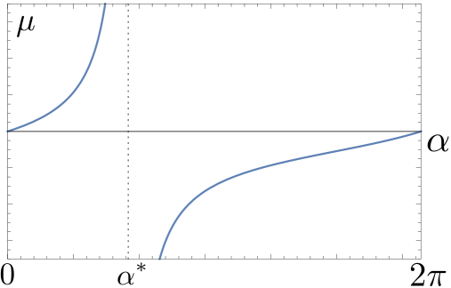
Figure 2: Plot of $\mu(\alpha)$ for the example used in Fig.1.

Newton cradle eigenvectors. Recall from above that in a Newton cradle every real number occurs exactly once as an eigenvalue, i.e., we have that for any $s\in\mathbb{R}$, there exists a pair $(n,\mu)$ so that $|s\rangle:=|s_{n}(\mu)\rangle$ obeys $S(\mu)|s\rangle=s|s\rangle$. The normalized eigenvectors $|s\rangle$ are defined only up to phases and so is their inner product. But the magnitude of their overlap is unique and we can prove that for all $s\in\mathbb{R}$:

$$\absolutevalue{\innerproduct{s}{s_{n}}}=\frac{\absolutevalue{v_{n}}}{\absolutevalue{s-s_{n}}}\left(\sum_{m=1}^{N}\frac{\absolutevalue{v_{m}}^{2}}{(s-s_{m})^{2}}\right)^{-1/2}$$ (15)

It is possible to choose the phases of the eigenvectors such that the overlap function $\langle s|s_{n}\rangle$ is real and continuous:

$$\innerproduct{s}{s_{n}}=\frac{(-1)^{n}\absolutevalue{v_{n}}}{s-s_{n}}\left(\sum_{m=1}^{N}\frac{\absolutevalue{v_{m}}^{2}}{(s-s_{m})^{2}}\right)^{-1/2}\prod_{r=1}^{N}\left(-1\right)^{\theta\left(s-s_{r}\right)}$$ (16)

Here, the singularity at $s=s_{n}$ is trivially removable and $\theta$ is the Heaviside function with $\theta(0):=0$. Using Eq. 16, the eigenvectors $|s_{n}(\mu)\rangle$ of the operators $S(\mu)=S+\mu|v\rangle\langle v|$ can be expressed explicitly in terms of the eigenvectors $|s_{k}\rangle$ of the operator $S$.
Iteration of Newton cradles to obtain $\bf{S+R}$. The Newton cradle for $|v\rangle:=|v^{(1)}\rangle$ and $\mu:=\mu^{(1)}$ yields the first step in the evolution of $S$ to $S+R$. For the second step, we need the coefficients $v^{(2)}_{n}$ of $|v^{(2)}\rangle$ in the eigenbasis $\{|s^{(1)}_{r}(\mu^{(1)})\rangle\}_{n=1}^{N}$ of the operator $S+\mu^{(1)}|v^{(1)}\rangle\langle v^{(1)}|$. Using Eq. 16, we obtain them exactly:

$$v^{(2)}_{n}=\langle s_{n}(\mu^{(1)})|v^{(2)}\rangle=\sum_{r=1}^{N}\langle s_{n}(\mu^{(1)})|s_{r}\rangle\langle s_{r}|v^{(2)}\rangle$$ (17)

Successively turning on all of the projectors that comprise $R$ yields $S+R$ as the result of $N$ Newton cradles.
Proofs. The key elements of the proofs are described in the Appendix. They are inspired by [11, 12, 13, 14, 15] and by von Neumann’s theory of the self-adjoint extensions of simple symmetric operators [16, 17], in particular for the case of deficiency indices $(1,1)$. Von Neumann’s theory itself does not apply in finite dimensions since in finite dimensions there are no symmetric non-self-adjoint operators. However, unitary extensions of isometries do exist in finite dimensions and, as we prove in the Appendix, they map, via the Cayley transform, into the addition of weighted projectors, rather than into the so-called abstract boundary conditions of von Neumann’s method.
Level repulsion. The important phenomenon of level repulsion, see, e.g., [18, 19], arises as a special case: Let us consider a $|v\rangle$ which obeys $v_{m}=\langle s_{m}|v\rangle=0$ for one $m$. Then the corresponding eigenvalue is frozen, $s_{m}(\mu)=s_{m}~{}\forall\mu$. The remaining eigenvalues $s_{n}(\mu)$ for $n\neq m$ form a Newton cradle and $s_{m-1}(\mu)$ will cross $s_{m}$ as $\mu$ runs from $0$ to $\infty$. In general, however, $|v_{m}|\neq 0$. In this case, no matter how small $|v_{m}|$ is, the eigenvalue $s_{m}(\mu)$ does participate in Newton’s cradle and is, therefore, not being crossed as $\mu$ runs. For very small $|v_{m}|$, the eigenvalue $s_{m-1}(\mu)$ can at most closely approach $s_{m}(\mu)$ while $s_{m}(\mu)$ barely moves until eventually $s_{m-1}(\mu)$ must repel $s_{m}(\mu)$ to send it on its way to $s_{m}^{*}$ as $\mu\rightarrow\infty$. Let us now consider the generating of the sum of two Hermitian operators, $S+R$, by successively continuously turning on one after the other of the weighted projectors that comprise $R$. Since each turning on of a weighted projector is a Newton cradle process, we conclude that the eigenvalues cannot cross during that process, i.e., we must have level repulsion, except when and only when the projector $|v^{(i)}\rangle\langle v^{(i)}|$ that is being added is orthogonal to an eigenvector of the operator that it is being added to.
Cauchy interlacing. The Cauchy interlacing theorem also arises as a special case. The theorem states that the $N-1$ eigenvalues $a_{1}<a_{2}<\ldots<a_{N-1}$ of any Hermitian $(N-1)\times(N-1)$ matrix $A$ obtained by deleting the $r$-th row ($r$ is arbitrary) and $r$-th column of a Hermitian $N\times N$ matrix $S$ with nondegenerate spectrum are interlaced in the $N$ eigenvalues of $S$, i.e.,: $s_{n}<a_{n}<s_{n+1}~{}\forall n=1\ldots(N-1)$. We can show that one obtains this result as the special case of the Newton cradle of $S$ in which $|v\rangle$ is chosen to be the vector with the components $\delta_{r,i}$ in the basis in which the matrix $S$ is given, and letting $\mu\rightarrow\infty$. Using Eq. 2 for $\mu\rightarrow\infty$, we can conclude more, namely that each of the interlaced eigenvalues $a_{n}$ is a solution of Eq. 3, which means that we can identify the interlaced eigenvalues as $a_{n}=s_{n}^{*}$ for $n=1,...~{},N-1$.
Generalization of Shannon sampling. Shannon sampling theory is central in information theory, where it establishes the equivalence of continuous and discrete representations of information [20, 21, 22, 23, 24]. Applied to physical fields, spacetime could be described as simultaneously discrete and continuous in the same way that information can, [12, 25, 26]. Shannon sampling also possesses a close relationship to generalized uncertainty principles [27, 11]. The basic Shannon sampling theorem [20] concerns $\Omega$-bandlimited functions, i.e., functions $f$ for which there exists an $\tilde{f}$ so that $f(s)=\int_{-\Omega}^{\Omega}e^{i\omega s}\tilde{f}(\omega)d\omega$. The theorem states that if the amplitudes $\{f(s_{n})\}_{n=-\infty}^{\infty}$ of an $\Omega$-bandlimited function $f$ on the real line are sampled at the so-called Nyquist spacing $\pi/\Omega$, e.g., $s_{n}:=n\pi/\Omega~{}~{}\forall n\in\mathbb{Z}$, then $f$ can be exactly reconstructed from these samples for all $s\in\mathbb{R}$:

$$f(s)=\sum_{n=-\infty}^{\infty}f(s_{n})~{}\frac{\sin(s\Omega-n\pi)}{s\Omega-n\pi}$$ (18)

While abundantly useful, this theorem has the drawbacks of assuming a constant bandwidth and a correspondingly constant Nyquist rate as well as requiring an infinite number of samples. In practice, these drawbacks can lead to inefficiencies and truncation errors respectively. In the literature, Shannon sampling has been generalized to varying Nyquist sampling rates, corresponding to varying bandwidths, see, e.g., [11, 15, 28]. These results still required taking infinitely many samples, the obstacle being the use of von Neumann’s method of self-adjoint extensions which does not apply in finite dimensions.

The present Newton cradle results are derived in finite dimensions and we now show that they can be applied to generalize Shannon sampling theory to enable both variable Nyquist rates and finite numbers of samples. To this end, let us assume given a Newton cradle, i.e., a family of Hermitian operators $S(\mu)=S+\mu|v\rangle\langle v|$ for fixed $S$, fixed $|v\rangle$ and for $\mu$ running through $\mathbb{R}$. We can then uniquely associate to every vector $|f\rangle$ in the Hilbert space the function $f(s):=\langle s|f\rangle$. These functions obey

$$f(s)=\langle s|f\rangle=\sum_{n=1}^{N}\langle s|s_{n}\rangle\langle s_{n}|f\rangle=\sum_{n=1}^{N}\langle s|s_{n}\rangle~{}f(s_{n}),$$ (19)

and more generally, for any $\mu$:

$$f(s)=\sum_{n=1}^{N}\langle s|s_{n}(\mu)\rangle~{}f(s_{n}(\mu))$$ (20)

Here, $\langle s|s_{n}(\mu)\rangle$ can be assumed real and continuous as given in Eq. 16. On one hand, Eqs. 19 and 20 reduce sampling theory to the fact that knowing the coefficients of a vector, $|f\rangle$, in the eigenbasis of one $S(\mu)$ implies knowing its coefficients in all bases, including the eigenbases of all other $S(\mu^{\prime})$. On the other hand, Eq. 20 shows that knowledge of the discrete set of amplitude samples $\{f(s_{n}(\mu))\}_{n=1}^{N}$ for a fixed $\mu$ suffices to reconstruct $f(s)$ for all $s\in\mathbb{R}$, establishing the equivalence of discrete and continuous representations of the information contained in $|f\rangle$. We can show that this result generalizes the sampling theory of [11, 15, 28] by allowing not only variable Nyquist rates but also finitely many samples without incurring truncation errors, while recovering the sampling results of [11, 15, 28] in the limit $N\rightarrow\infty$. In turn, [11, 15, 28] yield the Shannon sampling theorem [20] as the special case of an eternally constant Nyquist rate.

It will be interesting to explore applications of the new sampling result given in Eq. 16 and Eq. 19 in circumstances with known varying Nyquist rate, such as in synthetic aperture experiments. For example, in the planned SKA experiment [29], the effective bandwidth between a pair of antennas depends on their apparent distance as seen by the observed object and therefore varies predictably with the earth’s rotation. Since large communication costs demand maximally efficient data taking, the generalized Shannon sampling method could be useful by enabling sampling and reconstruction at continuously-adjusted Nyquist rates, without incurring truncation errors at the beginning and end of sample taking.
Algorithmic complexity in adiabatic quantum computing. Adiabatic quantum computing [30, 31] is polynomially equivalent [32] to algorithmic quantum computing [33] and is therefore in that sense as powerful. An adiabatic quantum computation starts at a time $t=0$ by preparing a system with a simple Hamiltonian, $H_{S}$, in its ground state. The Hamiltonian is then gradually changed from $H_{S}$ at $t=0$ to a different Hamiltonian $H_{C}$ at a time $t=T$ through $H(t):=(1-\frac{t}{T})H_{S}+\frac{t}{T}H_{C}$. Here, $H_{C}$ is a cost function Hamiltonian designed to implement the calculation by energetically penalizing errors. The ground state of $H_{C}$ represents the solution. For example, to implement a combinatorial satisfiability problem, e.g., from the NP-complete set of 3-SAT problems, [34], $H_{C}$ would be a sum of positive operators, $H_{C}=\sum_{i}H_{C,i}$, each of which implements a logical clause: a state $|\psi\rangle$ fulfils a clause $H_{C,i}$ iff it obeys $H_{C,i}|\psi\rangle=0$.

For an adiabatic quantum computation to succeed, the ground state $|E_{1}(t=0)\rangle$ of $H_{S}$ has to evolve between $t=0$ and $t=T$ into a state that matches the desired ground state $|E_{1}(t=T)\rangle$ of $H_{C}$ with high fidelity. By the adiabatic theorem, see, e.g., [30], this is achieved if the process of switching over from $H_{S}$ to $H_{C}$ is slow enough: $T\gg\frac{a}{g_{min}^{2}}$. Here, $a$ is the transition matrix element $a:=\max_{0\leq t\leq T}|\langle E_{2}(t)|H_{C}-H_{S}|E_{1}(t)\rangle|$ and $g_{min}$ is the minimum of the spectral gap $E_{2}(t)-E_{1}(t)$ of $H(t)$ over the ground state as $t$ runs from $t=0$ to $t=T$. The dominant behavior is that the smaller the spectral gap, the more time, $T$, is needed for the computation.

The question arises as to what it is that makes an adiabatic quantum computation problem computationally complex, in the sense that only a slow evolution will let the ground state of the simpler system $H_{S}$ adiabatically evolve into the desired ground state of $H_{C}$. In particular, what properties of the cost function Hamiltonian $H_{C}$ and the low lying states of the Hamiltonian $H_{S}$ cause the gap to narrow during the computation?

For a preliminary application of the Newton cradle results, we write $H(t)=S+\frac{t}{T}R$ where $S:=H_{S}$ and $R:=H_{C}-H_{S}$. Without incurring significant overhead, we can turn on $R$ by changing only one at a time of the prefactors $\mu^{(n)}$ of the projectors $|v^{(n)}\rangle\langle v^{(n)}|$ that comprise $R$. Let us now focus on one of these intermediate steps in the adiabatic quantum computation, say a step in which the prefactor $\mu^{(n)}$ of the projector $|v^{(n)}\rangle\langle v^{(n)}|$ is being increased. (In the example of satisfiability problems, we may intuitively think of this as adding a new clause.) The ground and first excited states at the beginning of this step shall be called $|g\rangle$ and $|e\rangle$.

The question now is what property of $|g\rangle$, $|e\rangle$ and the projector $|v^{(n)}\rangle\langle v^{(n)}|$ determines whether the gap narrows during the computation, i.e., whether the addition of $\mu^{(n)}|v^{(n)}\rangle\langle v^{(n)}|$ increases the computational complexity in the sense that it slows down the computation.

From the behavior of Newton cradles, we know that as a prefactor $\mu^{(n)}$ is being increased, all eigenvalues increase. Therefore, the gap over the ground state narrows iff the ground state eigenvalue increases faster than the first exited state’s eigenvalue. From Eq. 5, we know that $ds_{1}/d\mu^{(n)}=|v_{1}^{(n)}|^{2}=|\langle g|v^{(n)}\rangle|^{2}$ and $ds_{2}/d\mu^{(n)}=|v_{2}^{(n)}|=|\langle e|v^{(n)}\rangle|^{2}$. Therefore, the gap narrows iff:

$$|\langle g|v^{(n)}\rangle|^{2}>|\langle e|v^{(n)}\rangle|^{2}$$ (21)

Defining $H^{(n)}:=\mu^{(n)}|v^{(n)}\rangle\langle v^{(n)}|$, Eq. 21 becomes:

$$\langle g|H^{(n)}|g\rangle>\langle e|H^{(n)}|e\rangle$$ (22)

Therefore, at any point within an adiabatic quantum computation, the addition of a new contribution $H^{(n)}:=\mu^{(n)}|v^{(n)}\rangle\langle v^{(n)}|$ to the Hamiltonian is algorithmically complex in the sense that a slight increase in $\mu^{(n)}$ narrows the gap and therefore forces a slowdown of the computation if and only if $H^{(n)}$ energetically penalizes the current ground state $|g\rangle$ more than the current first excited state, $|e\rangle$, i.e., iff the current ground state fulfills the condition posed by $H^{(n)}$ less than the current first excited state does. This indicates that it is desirable, for example, to choose an $H_{S}$ whose ground state is a better approximation to the solution than its low lying states.

While Eq.22 could be obtained from first order perturbation, the nonperturbative Newton cradle results may also enable a nonperturbative analysis for the full time evolution. First, Eq. 4 yields the eigenvalue velocities and accelerations for all $s$. An analysis that takes into account the Newton cradles of all projectors comprising $R$, could, therefore, yield nonperturbative insights into when, where and why the eigenvalue traffic on the $s$-axis decelerates and, therefore, leads to the narrowing of gaps between eigenvalues. Second, given knowledge of the evolving eigenvalues, Eq. 16 yields nonperturbative information on the evolution of the eigenvectors, including the ground state. In this context, it should also be very interesting to explore the role of the Newton cradle mechanism in Quantum Approximate Optimization Algorithms (QAOA), [35, 36].

For completeness, we add that the turning on of the projectors comprising $R$ can generate not only right-moving but also left-moving Newton cradles. This is because even with $H_{S}$ and $H_{C}$ positive, $R=H_{C}-H_{S}$ may not be positive and can possess positive as well as negative eigenvalues $\mu^{(n)}$. For negative $\mu^{(n)}$, the gap narrows if the leftward speed of the ground state is smaller than that of the first excited state, i.e., if $|\langle g|v\rangle|^{2}<|\langle e|v\rangle|^{2}$. Since $\mu^{(n)}<0$, this yields again Eq. 22.
Outlook. Dynamics of quantum channels. Quantum channels are established through physical interactions and the question arises as to how the quantum channel capacity, i.e., the channel’s ability to transmit entanglement or coherent information, depends on the dynamics of the interactions involved. The dynamics of the negativities and coherent information are functions of the dynamics of the spectra of density operators and their partial transpose. Building on [37], decomposing the dynamics of interactions into Newton cradles may, therefore, yield new insight into the establishing of quantum channel capacities in interactions.
Casimir-like forces. Newton cradle decompositions should also be interesting to apply to the analysis of the dynamics of the spectra, and therefore the ground state energies, of quantum field mode decompositions under the variation of classical parameters, [38, 39], leading to effective forces. An example is the Casimir force that arises when the parameters describe the distances and shapes of conductors, such as parallel conducting plates [40, 41]. Another example is the inducing of gravitational forces in Sakharov’s approach [42].
Generalization to infinite-dimensional Hilbert spaces. The present results apply in finite-dimensional Hilbert spaces and, for this case, it should be very interesting to apply them also, for example, to random matrix theory [43] where they could help shed light on the dynamics of the BBT transition [44, 45] in quantum chaotic systems. In infinite-dimensional Hilbert spaces, the Cayley transform of the unitaries $U(\alpha)$ can yield bounded or unbounded self-adjoint operators. In the unbounded case, von Neumann’s theory of self adjoint extensions can be applied and it shows that the operators $S(\mu)$ differ not by a multiple of a projector but a domain extension, such as boundary conditions in the case of differential operators [17], though interestingly they can differ by a self-adjoint operator by using an auxiliary Hilbert space [46]. For the resulting generalization of Shannon sampling see, e.g., [11, 15, 27, 28]. It will be interesting to explore the generalization of the present results in the limit $N\rightarrow\infty$ and to families of bounded operators, $S(\mu)$, in infinite-dimensions, i.e., for finite-size Newton cradles with infinitely many eigenvalues.
Spectral geometry. Spectral geometry asks to what extent the spectra of Hermitian Laplacian and Dirac operators on Riemannian manifolds determine the metric of the manifold, see, e.g., [47]. Spectral geometric methods have also been applied to bridge between the differential geometric language of general relativity and the functional analytic language of quantum theory [13, 48, 49]. In this context, a Newton cradle analysis could yield new insights into the dynamics of the spectra of Laplacian and Dirac operators as a function of parametrized changes to the metric of manifolds.

Acknowledgements. The authors are grateful for valuable feedback on the manuscript from José Polo Gómez, Jason Pye, Marcus Reitz, Koji Yamaguchi and Eduardo Martín-Martínez. AK acknowledges support through a Discovery Grant of the National Science and Engineering Council of Canada (NSERC), a Discovery Project grant of the Australian Research Council (ARC) and a Google Faculty Research Award. BŠ is supported in part by the Perimeter Institute, which is supported in part by the Government of Canada through the Department of Innovation, Science and Economic Development Canada and by the Province of Ontario through the Ministry of Economic Development, Job Creation and Trade.

Appendix

Here, we describe the key elements of the proofs. To this end, we map self-adjoint to unitary operators, and vice versa, using the Cayley transform. An advantage of the Cayley transform is that, unlike exponentiation, the Cayley transform is bijective and hence uniquely invertible. Since we work here in finite-dimensional Hilbert spaces, the terms Hermitian and self-adjoint can be used interchangeably.

I Relation between Hermitian and unitary Newton cradles

We claim that the left action of a representation of the unitary group $U(1)$ on a unitary operator $U$ is mapped, via the Cayley transform, into the addition of multiples of a rank $1$ projector to a Hermitian operator $S$. Concretely, assume $U$ is an arbitrary fixed unitary acting on a finite-dimensional Hilbert space $\cal{H}$. Then its Cayley transform is defined to be the Hermitian operator $S$:

$$S:=-i\left(U+\mathbb{1}\right)\left(U-\mathbb{1}\right)^{-1}$$ (23)

We multiply $U$ from the left with an element of the $U(1)$-family of unitaries $(\mathbb{1}+\left(e^{i\alpha}-1\right)\ket{w}\bra{w})$ where $|w\rangle$ is an arbitrary fixed normalized vector. Running through all $\alpha\in[0,2\pi)$, we obtain a family of unitaries $U(\alpha)$:

$$U(\alpha):=U+\left(e^{i\alpha}-1\right)\ket{w}\bra{w}U$$ (24)

By Cayley transforming each of the $U(\alpha)$, we obtain a family of self-adjoint operators $S(\alpha)$

$$S({\alpha}):=-i\left(U({\alpha})+\mathbb{1}\right)\left(U({\alpha})-\mathbb{1}\right)^{-1}$$ (25)

with $S(0)=S$. We claim that, for any fixed choice of $U$ and $|w\rangle$, the Hermitian operators $S(\alpha)$ for varying $\alpha$ differ by a multiple of a rank $1$ projector, i.e., that there exists a normalized vector $|v\rangle$ so that for every $\alpha\in[0,2\pi)$ there exists a $\mu(\alpha)\in\mathbb{R}$ obeying:

$$S(\mu(\alpha))=S+\mu|v\rangle\langle v|$$ (26)

For the proof, we start with:

$$S(\alpha) = -i\left(\mathbb{1}+U+\left(e^{i\alpha}-1\right)\ket{w}\bra{w}U\right)$$ (28)

$$\times\left(U+\left(e^{i\alpha}-1\right)\ket{w}\bra{w}U-\mathbb{1}\right)^{-1}$$

Acting from the right with the operator $\left(U+\left(e^{i\alpha}-1\right)\ket{w}\bra{w}U-\mathbb{1}\right)$ yields:

$$S(\alpha)\left(U+\left(e^{i\alpha}-1\right)\ket{w}\bra{w}U-\mathbb{1}\right)$$

$$\mbox{~{}~{}~{}~{}~{}~{}~{}~{}~{}~{}~{}~{}~{}}=-i\left(1+U\right)-i\left(e^{i\alpha}-1\right)\ket{w}\bra{w}U$$ (29)

Rearranging the terms:

$$S(\alpha)\left(U-\mathbb{1}\right)+S(\alpha)\left(e^{i\alpha}-1\right)\ket{w}\bra{w}U$$

$$\mbox{~{}~{}~{}~{}~{}~{}~{}~{}~{}}=-i\left(1+U\right)-i\left(e^{i\alpha}-1\right)\ket{w}\bra{w}U$$ (30)

After acting with the operator $\left(U-\mathbb{1}\right)^{-1}$ from the right we recognize the expression for the Cayley transform $S$ of $U$ and obtain:

$$S(\alpha)-S=-\left(S(\alpha)+i\right)\left(e^{i\alpha}-1\right)\ket{w}\bra{w}U\left(U-\mathbb{1}\right)^{-1}.$$ (31)

Since both $S(\alpha)$ and $S$ are self-adjoint operators, their difference, $S(\alpha)-S$, is also self-adjoint. This means that the following equation must hold for some $\mu^{\prime}\left(\alpha\right)\in\mathbb{R}$:

$$-\left(S(\alpha)+i\right)\left(e^{i\alpha}-1\right)\ket{w}=\mu^{\prime}\left(\alpha\right)\left[\left(U-\mathbb{1}\right)^{-1}\right]^{\dagger}U^{\dagger}\ket{w}.$$ (32)

The left $U(1)$ action on the unitary $U$ which results in $U(\alpha)$ therefore corresponds to the addition of a multiple of a projector $\mu\left(\alpha\right)\ket{v}\bra{v}$ to $S$, resulting in

$$S(\alpha)=S+\mu\left(\alpha\right)\ket{v}\bra{v},$$ (33)

where:

$$\ket{v}=\frac{1}{\mathcal{N}_{v}}\left(U^{\dagger}-\mathbb{1}\right)^{-1}U^{\dagger}\ket{w}$$ (34)

Calculating the norm of Eq. 34 while inserting a resolution of the identity, the normalization constant $\mathcal{N}_{v}$ follows:

$$\mathcal{N}_{v}=\sqrt{\sum_{m}\frac{\absolutevalue{w_{m}}^{2}}{\absolutevalue{u_{m}-1}^{2}}}=\frac{\sqrt{\sum_{m}\absolutevalue{w_{m}}^{2}\left(s_{m}^{2}+1\right)}}{2}.$$ (35)

Recall that we use the notation $w_{n}:=\langle s_{n}|w\rangle,v_{n}:=\langle s_{n}|v\rangle$ and $U(\alpha)|u_{n}(\alpha)\rangle=u_{n}(\alpha)|u_{n}(\alpha)\rangle,~{}~{}S(\mu)|s_{n}(\mu)\rangle=s_{n}(\mu)|s_{n}(\mu)\rangle$.

II Relating the eigenbases of $U(\alpha)$ and $S(\alpha)$ to those of $U$ and $S$

Our aim is to construct the eigenvectors of $U(\alpha)$ (and therefore of $S(\mu)$) in terms of the eigenbasis of $U$ (and $S$). We have

$$\begin{split}u_{n}(\alpha)\innerproduct{u_{n}(\alpha)}{u_{m}}&=\bra{u_{n}(\alpha)}U(\alpha)\ket{u_{m}}\\ &=\bra{u_{n}(\alpha)}(U+(e^{i\alpha}-1)\ket{w}\bra{w}U)\ket{u_{m}}\\ &=\innerproduct{u_{n}(\alpha)}{u_{m}}u_{m}\\ &~{}~{}~{}+(e^{i\alpha}-1)\innerproduct{u_{n}(\alpha)}{w}\innerproduct{w}{u_{m}}u_{m},\end{split}$$ (36)

and therefore:

$$\innerproduct{u_{n}(\alpha)}{u_{m}}=(e^{i\alpha}-1)\innerproduct{u_{n}(\alpha)}{w}~{}\frac{\innerproduct{w}{u_{m}}u_{m}}{u_{n}(\alpha)-u_{m}}$$ (37)

Using

$$1=\innerproduct{u_{n}(\alpha)}{u_{n}(\alpha)}=\sum_{m}\innerproduct{u_{n}(\alpha)}{u_{m}}\innerproduct{u_{m}}{u_{n}(\alpha)},$$ (38)

we obtain:

$$1=|e^{-i\alpha}-1|^{2}|\innerproduct{u_{n}(\alpha)}{w}|^{2}\sum_{m}\frac{\absolutevalue{u_{m}}^{2}\absolutevalue{\innerproduct{w}{u_{m}}}^{2}}{\absolutevalue{u_{n}(\alpha)-u_{m}}^{2}}$$ (39)

This means that, in Eq. 37, we can express $\absolutevalue{(e^{i\alpha}-1)\innerproduct{u_{n}(\alpha)}{w}}$ in terms of known quantities to obtain:

$$\absolutevalue{\innerproduct{u_{n}(\alpha)}{u_{m}}}=\absolutevalue{\frac{\innerproduct{w}{u_{m}}}{u_{n}(\alpha)-u_{m}}}\quantity(\sum_{k}\frac{\absolutevalue{\innerproduct{w}{u_{k}}}^{2}}{\absolutevalue{u_{n}(\alpha)-u_{k}}^{2}})^{-1/2}.$$ (40)

Via the Cayley transform, this yields:

$$\absolutevalue{\innerproduct{s}{s_{n}}}=\frac{\absolutevalue{v_{n}}}{\absolutevalue{s-s_{n}}}\left(\sum_{k}\frac{\absolutevalue{v_{k}}^{2}}{(s-s_{k})^{2}}\right)^{-1/2}$$ (41)

Further, the overlap function $\langle s|s_{n}\rangle$ can be chosen real for all $s,s_{n}$ by suitably choosing the phases of the eigenvectors $|s\rangle$. To see this, we calculate:

$$\frac{s_{r}(\alpha)-i}{s_{r}(\alpha)+i}\langle s_{n}|s_{r}(\alpha)\rangle=\langle s_{n}|U(\alpha)|s_{r}(\alpha)\rangle$$ (42)

$$=\langle s_{n}|\left(\mathbb{1}+(e^{i\alpha}-1)|w\rangle\langle w|\right)U|s_{r}(\alpha)\rangle$$ (43)

$$=\frac{s_{n}-i}{s_{n}+i}\langle s_{n}|s_{r}(\alpha)\rangle+(e^{i\alpha}-1)\langle s_{n}|w\rangle\langle w|U|s_{r}(\alpha)\rangle$$ (44)

This equation can be rewritten as

$$\langle s_{n}|s_{r}(\alpha)\rangle=\frac{g_{n}M(s_{r}(\alpha))}{s_{r}(\alpha)-s_{n}}$$ (45)

where we separated the $n$-dependent from the $s$-dependent terms by defining:

$$g_{n}:=(s_{n}+i)\langle s_{n}|w\rangle$$ (46)

$$M(s_{r}(\alpha)):=\frac{(s_{r}(\alpha)+i)}{2i}(e^{i\alpha}-1)\langle w|U|s_{r}(\alpha)\rangle$$ (47)

We use the choice of phases of the eigenvectors $|s_{n}\rangle=|s_{n}(\alpha=0)\rangle$ so that $g_{n}\in\mathbb{R}$ for all $n$. Further, we choose the phases of the eigenvectors $|s_{r}(\alpha)\rangle$ for $\alpha\neq 0$ such that $M(t_{r}(\alpha))\in\mathbb{R}$ for all $\alpha\neq 0$. Notice that $M(t_{r}(\alpha))=0$ for $\alpha=0$. While these choices ensure that $\langle s_{n}|s_{r}(\alpha)\rangle\in\mathbb{R}$, the overlap function can also be made continuous through a suitable choice of signs, as described in the main text.

III Velocity of the complex eigenvalues

Differentiating Eq. 36 at $\alpha=0$ for $n=m$, yields:

$$\left.\frac{du_{n}(\alpha)}{d\alpha}\right|_{\alpha=0}=i~{}|\langle u_{n}|w\rangle|^{2}u_{n}$$ (48)

Since, for any $\alpha$, we could choose $U(\alpha)$ to be the starting unitary $U$ of a new Newton cradle with $|v\rangle$, the velocity of the complex eigenvalues for all $\alpha$ reads:

$$\frac{\differential u_{n}\left(\alpha\right)}{\differential\alpha}=i\absolutevalue{\innerproduct{u_{n}\left(\alpha\right)}{u_{n}\left(\alpha\right)}{w}}^{2}u_{n}\left(\alpha\right).$$ (49)

From Eq. 39, we have:

$$\absolutevalue{\innerproduct{u_{n}\left(\alpha\right)}{u_{n}\left(\alpha\right)}{w}}^{2}=\frac{1}{\absolutevalue{e^{i\alpha}-1}^{2}}\quantity(\sum_{m}\frac{\absolutevalue{w_{m}}^{2}}{\absolutevalue{u_{n}(\alpha)-u_{m}}^{2}})^{-1}.$$ (50)

Therefore, Eq. 49 becomes this differential equation:

$$\frac{\differential u_{n}(\alpha)}{\differential\alpha}=iu_{n}(\alpha)\frac{1}{\absolutevalue{e^{i\alpha}-1}^{2}}\quantity(\sum_{m}\frac{\absolutevalue{w_{m}}^{2}}{\absolutevalue{u_{n}(\alpha)-u_{m}}^{2}})^{-1}$$ (51)

IV Velocity of the real eigenvalues

The Möbius transform $u_{k}=(s_{k}-i)/(s_{k}+i)$ yields for the real eigenvalues of $S(\alpha)$:

$$\frac{ds_{n}}{d\alpha}=\frac{(s_{n}+i)^{2}}{2i}\frac{du_{n}}{d\alpha}.$$ (52)

The inverse Möbius transform $s_{k}=i(1+u_{k})/(1-u_{k})$, applied to Eq. 40, then yields for the real eigenvalues $\{s_{n}\}_{n\in 1,...,N}$:

$$\frac{\differential s_{n}}{\differential\alpha} =\frac{1}{2}\frac{1}{\absolutevalue{e^{i\alpha}-1}^{2}}\quantity(\sum_{m}\absolutevalue{w_{m}}^{2}\frac{s_{m}^{2}+1}{4(s_{n}-s_{m})^{2}})^{-1}$$

$$=\frac{1}{2}\frac{1}{\sin^{2}(\frac{\alpha}{2})}\quantity(\sum_{m}\absolutevalue{w_{m}}^{2}\frac{s_{m}^{2}+1}{(s_{n}-s_{m})^{2}})^{-1}$$ (53)

V Integrating the differential equation for the velocities

After separating the variables $s_{n}$ and $\alpha$,

$$\differential s_{n}\sum_{m}\absolutevalue{w_{m}}^{2}\frac{s_{m}^{2}+1}{(s_{n}-s_{m})^{2}}=\frac{\differential\alpha}{2\sin^{2}(\frac{\alpha}{2})},$$ (54)

integrating with the initial conditions $s_{n}\left(\alpha=0\right)=s_{n}$ yields:

$$\sum_{m}\absolutevalue{w_{m}}^{2}\frac{s_{m}^{2}+1}{s_{n}(\alpha)-s_{m}}+\sum_{m}\absolutevalue{w_{m}}^{2}s_{m}=\cot(\frac{\alpha}{2})$$ (55)

As expected, since this yields a polynomial of order $n$ in $s_{n}(\alpha)$, there are $N$ solutions $\{s_{n}(\alpha)\}_{n=1,...,N}$.

In order to express Eq. 55 using the components of $\ket{v}$ rather than $\ket{w}$, we express $\ket{w}$ in terms of $\ket{v}$ and the operator $U$:

$$\ket{w}=\mathcal{N}_{v}\ U\left(U^{\dagger}-\mathbb{1}\right)\ket{v}=\mathcal{N}_{v}\left(\mathbb{1}-U\right)\ket{v}$$ (56)

To obtain the components of $\ket{w}$ and $\ket{v}$, we act with $\bra{u_{k}}$ from the left:

$$w_{k}=\innerproduct{u_{k}}{w}=\mathcal{N}_{v}\bra{u_{k}}\left(\mathbb{1}-U\right)\ket{v},$$ (57)

$$w_{k}=\mathcal{N}_{v}\left(1-u_{k}\right)v_{k}$$ (58)

Since only the absolute values of $w_{k}$ appear in Eq. 55, we calculate $\absolutevalue{w_{k}}^{2}$ and then inverse Cayley transform $u_{k}$ in order to get an expression that depends on the real eigenvalues $\{s_{i}\}_{i=1,...,N}$:

$$\absolutevalue{w_{k}}^{2} = \absolutevalue{\mathcal{N}_{v}}^{2}\absolutevalue{1-u_{k}}^{2}\absolutevalue{v_{k}}^{2}$$ (59)

$$= \absolutevalue{\mathcal{N}_{v}}^{2}\frac{4}{s_{k}^{2}+1}\absolutevalue{v_{k}}^{2}.$$ (60)

This yields Eq. 55 in terms of the $v_{k}$:

$$\cot(\frac{\alpha}{2}) = \sum_{m}4\absolutevalue{\mathcal{N}_{v}}^{2}\frac{\absolutevalue{v_{m}}^{2}}{s_{n}(\alpha)-s_{m}\left(0\right)}$$ (61)

$$+\sum_{m}\absolutevalue{v_{m}}^{2}4\absolutevalue{\mathcal{N}_{v}}^{2}\frac{s_{m}}{s_{m}^{2}+1}s_{m}$$

VI The relationship between $\mu$ and $\alpha$

We claim that $\mu\left(\alpha\right)$ is given by:

$$\mu\left(\alpha\right)=\sum_{m}\absolutevalue{w_{m}}^{2}\left(s_{m}^{2}+1\right)\left(\cot\left(\frac{\alpha}{2}\right)-\sum_{m}\absolutevalue{w_{m}}^{2}s_{m}\right)^{-1}$$ (62)

We start the proof with the observation that $S(\alpha)-S=\mu|v\rangle\langle v|$ yields:

$$\left(s_{n}(\alpha)-s_{m}\right){\innerproduct{s_{m}}{s_{n}\left(\alpha\right)}}=\mu\left(\alpha\right){\innerproduct{s_{m}}{v}\innerproduct{v}{s_{n}\left(\alpha\right)}}$$ (63)

We solve this equation for $\left(s_{n}(\alpha)-s_{m}\right)$ and substitute it into Eq. 55 to obtain:

$$\frac{1}{\mu}\sum_{m}\absolutevalue{w_{m}}^{2}\left(s_{m}^{2}+1\right)\frac{\innerproduct{s_{m}}{s_{n}\left(\alpha\right)}}{\innerproduct{s_{m}}{v}\innerproduct{v}{s_{n}\left(\alpha\right)}}$$ (64)

$$~{}~{}~{}~{}~{}=\cot\left(\frac{\alpha}{2}\right)-\sum_{m}\absolutevalue{w_{m}}^{2}s_{m}$$ (65)

From Eq. 34, a Möbius transform yields

$$\innerproduct{s_{m}}{v}=\frac{1}{\mathcal{N}_{v}}\frac{s_{m}+i}{2i}\innerproduct{s_{m}}{w},$$ (66)

i.e.,

$$\left(s_{m}+i\right)w_{m}=2i\ \mathcal{N}_{v}\ v_{m}.$$ (67)

Substituting this expression into Eq.64, we obtain:

$$\frac{1}{\mu}\sum_{m}2i\ \mathcal{N}_{v}\left(s_{m}-i\right)w_{m}^{*}\frac{\innerproduct{s_{m}}{s_{n}\left(\alpha\right)}}{\innerproduct{v}{s_{n}\left(\alpha\right)}}$$

$$~{}~{}~{}~{}~{}=\cot\left(\frac{\alpha}{2}\right)-\sum_{m}\absolutevalue{w_{m}}^{2}s_{m}.$$ (68)

We now insert a resolution of the identity $\mathbb{1}=\sum_{m}\ket{s_{m}}\bra{s_{m}}$ into the inner product $\innerproduct{s_{n}(\alpha)}{v}$ and use Eq. 34 to obtain:

$$\innerproduct{s_{n}\left(\alpha\right)}{v}=\frac{1}{\mathcal{N}_{v}}\sum_{m}\innerproduct{s_{n}\left(\alpha\right)}{s_{m}}\innerproduct{s_{m}}{w}\frac{u_{m}^{*}}{u_{m}^{*}-1}$$ (69)

We then divide by $\innerproduct{s_{n}(\alpha)}{v}$ and complex conjugate the entire expression:

$$1=\frac{1}{\mathcal{N}_{v}}\sum_{m}w_{m}^{*}\frac{s_{m}-i}{-2i}\frac{\innerproduct{s_{m}}{s_{n}\left(\alpha\right)}}{\innerproduct{v}{s_{n}\left(\alpha\right)}}$$ (70)

Now we recognize the same sum as in Eq. VI, up to constants, so we can finally express $\mu$ as a function of $\alpha$:

$$\mu=4\mathcal{N}_{v}^{2}\left(\cot\left(\frac{\alpha}{2}\right)-\sum_{m}\absolutevalue{w_{m}}^{2}s_{m}\right)^{-1}$$ (71)

With ${\mathcal{N}_{v}}$ given in Eq. 35, this yields Eq. 62 as claimed.

VII Reformulation of the characteristic equation of $S(\mu)$

We now derive the equation:

$$\sum_{m}\frac{\absolutevalue{v_{m}}^{2}}{s_{n}(\mu)-s_{m}}=\frac{1}{\mu}.$$ (72)

To this end, we use $\absolutevalue{w_{k}}^{2}=\absolutevalue{\mathcal{N}_{v}}^{2}\frac{4}{s_{k}^{2}+1}\absolutevalue{v_{k}}^{2}$to express $w_{m}$ in terms of $v_{m}$ in Eq. 55:

$$4\absolutevalue{\mathcal{N}_{v}}^{2}\sum_{m}\frac{\absolutevalue{v_{m}}^{2}}{s_{n}(\alpha)-s_{m}}=\cot(\frac{\alpha}{2})-\sum_{m}\absolutevalue{w_{m}}^{2}s_{m},$$ (73)

Using Eq. 71, we express the right-hand side in Eq.73 in terms of $\mu(\alpha)$:

$$4\absolutevalue{\mathcal{N}_{v}}^{2}\sum_{m}\frac{\absolutevalue{v_{m}}^{2}}{s_{n}(\alpha)-s_{m}}=4\absolutevalue{\mathcal{N}_{v}}^{2}\frac{1}{\mu(\alpha)}.$$ (74)

Finally, dividing by $4\absolutevalue{\mathcal{N}_{v}}^{2}$, and expressing the dependence on $\alpha$ as a dependence on $\mu$, we obtain Eq.72. We remark that an equation equivalent to Eq.72, which is equivalent to the characteristic equation $\det(S(\mu)-s\mathbb{1})=0$ of $S(\mu)$, was used in [50] to derive a numerical algorithm for the eigenvalue problem, along with a perturbative stability analysis.

References

Strang [2016]G. Strang, Introduction to Linear
Algebra (Wellesley-Cambridge Press, 2016).
Davis and Thomson [2000]H. Davis and K. T. Thomson, Linear Algebra and
Linear Operators in Engineering: With Applications in Mathematica, ISSN (Elsevier Science, 2000).
Norman and Wolczuk [2011]D. Norman and D. Wolczuk, Introduction to Linear
Algebra for Science and Engineering (Pearson, 2011).
Von Neumann and Wigner [1929]J. Von Neumann and E. Wigner, Z.
Phys 30, 467 (1929).
Hsu and Angles d’Auriac [1993]T. C. Hsu and J. Angles d’Auriac, Physical Review B 47, 14291 (1993).
Chou and Foster [2014]Y.-Z. Chou and M. S. Foster, Physical Review B 89, 165136 (2014).
Cauchy [1829]A.-L. Cauchy, Complete Works (Serie 2) 9 (1829).
De la Sen [2019]M. De la Sen, Symmetry 11, 712
(2019).
Bonfiglioli and Fulci [2011]A. Bonfiglioli and R. Fulci, Topics in noncommutative
algebra: the theorem of Campbell, Baker, Hausdorff and Dynkin, Vol. 2034 (Springer Science &
Business Media, 2011).
Akhiezer and Glazman [2013]N. I. Akhiezer and I. M. Glazman, Theory of Linear
Operators in Hilbert Space, Dover Books on Mathematics (Dover Publications, 2013).
Plumb et al. [2016]K. Plumb, K. Hwang,
Y. Qiu, L. W. Harriger, G. Granroth, A. I. Kolesnikov, G. Shu, F. Chou, C. Rüegg, Y. B. Kim,
et al., Nature Physics 12, 224
(2016).
Arias et al. [2003]J. Arias, J. Dukelsky, and J. García-Ramos, Physical Review Letters 91, 162502 (2003).
Shannon [1948]C. E. Shannon, The
Bell System Technical Journal 27, 379 (1948).
Jerri [1977]A. J. Jerri, Proceedings of the IEEE 65, 1565 (1977).
Marks [2012]R. J. I. Marks, Introduction
to Shannon sampling and interpolation theory (Springer Science & Business Media, 2012).
Zayed [2018]A. I. Zayed, Advances in Shannon’s
sampling theory (Routledge, 2018).
Benedetto and Ferreira [2001]J. J. Benedetto and P. J. Ferreira, Modern sampling
theory: Mathematics and Applications (Springer
Science & Business Media, 2001).
Kempf [2010]A. Kempf, New
Journal of Physics 12, 115001 (2010).
Chatwin-Davies et al. [2017]A. Chatwin-Davies, A. Kempf, and R. T. Martin, Physical Review Letters 119, 031301 (2017).
Kempf [1994]A. Kempf, Journal
of Mathematical Physics 35, 4483 (1994).
Martin and Kempf [2009]R. Martin and A. Kempf, Acta Applicandae
Mathematicae 106, 349
(2009).
Wang et al. [2015]B. Wang, X. Zhu, C. Gao, Y. Bai, J. Dong, and L. Wang, Scientific reports 5, 1 (2015).
Farhi et al. [2000]E. Farhi, J. Goldstone,
S. Gutmann, and M. Sipser, Quantum computation by adiabatic evolution (2000), arXiv:quant-ph/0001106 [quant-ph] .
Aharonov et al. [2008]D. Aharonov, W. Van Dam,
J. Kempe, Z. Landau, S. Lloyd, and O. Regev, SIAM Review 50, 755 (2008).
Nielsen and Chuang [2002]M. A. Nielsen and I. Chuang, Quantum computation and
quantum information (American Association of
Physics Teachers, 2002).
Farhi et al. [2001]E. Farhi, J. Goldstone,
S. Gutmann, J. Lapan, A. Lundgren, and D. Preda, Science 292, 472 (2001).
Farhi et al. [2014]E. Farhi, J. Goldstone, and S. Gutmann, arXiv preprint
arXiv:1411.4028 (2014).
Zhou et al. [2020]L. Zhou, S.-T. Wang,
S. Choi, H. Pichler, and M. D. Lukin, Physical Review X 10, 021067 (2020).
Kendall et al. [2022]E. Kendall, B. Šoda, and A. Kempf, Journal
of Physics A: Mathematical and Theoretical 55, 255301 (2022).
Fulling [1989]S. A. Fulling, Aspects of quantum
field theory in curved spacetime, 17 (Cambridge University Press, 1989).
Birrell et al. [1984]N. D. Birrell, N. D. Birrell, and P. Davies, Quantum fields in curved
space (Cambridge University Press, 1984).
Casimir [1948]H. B. G. Casimir, Indag. Math. 10, 261 (1948).
Milton [2009]K. Milton, Journal of Physics: Conference Series 161, 012001 (2009).
Sakharov [2000]A. D. Sakharov, General Relativity and Gravitation 32, 365 (2000).
Guhr et al. [1998]T. Guhr, A. Müller-Groeling, and H. A. Weidenmüller, Physics Reports 299, 189 (1998).
Baik et al. [2005]J. Baik, G. B. Arous, and S. Péché, The Annals of
Probability 33, 1643
(2005).
Péché [2006]S. Péché, Probability Theory and Related Fields 134, 127 (2006).
Posilicano [2003]A. Posilicano, Annali della Scuola Normale Superiore di Pisa-Classe di Scienze 2, 1 (2003).
Datchev and Hezari [2011]K. Datchev and H. Hezari, Inverse problems and applications: Inside Out II 60, 455 (2011).
Aasen et al. [2013]D. Aasen, T. Bhamre, and A. Kempf, Physical Review Letters 110, 121301 (2013).
Kempf [2021]A. Kempf, Frontiers in Physics 9, 655857 (2021).
Bunch et al. [1978]J. R. Bunch, C. P. Nielsen, and D. C. Sorensen, Numerische
Mathematik 31, 31
(1978).