The Hubble Space Telescope UV Legacy Survey of Galactic Globular Clusters. XXIII. Proper-motion catalogs and internal kinematics.

Abstract

A number of studies based on the data collected by the Hubble Space Telescope (HST) GO-13297 program “HST Legacy Survey of Galactic Globular Clusters: Shedding UV Light on Their Populations and Formation” have investigated the photometric properties of a large sample of Galactic globular clusters and revolutionized our understanding of their stellar populations. In this paper, we expand upon previous studies by focusing our attention on the stellar clusters’ internal kinematics. We computed proper motions for stars in 56 globular and one open clusters by combining the GO-13297 images with archival HST data. The astro-photometric catalogs released with this paper represent the most complete and homogeneous collection of proper motions of stars in the cores of stellar clusters to date, and expand the information provided by the current (and future) Gaia data releases to much fainter stars and into the crowded central regions. We also census the general kinematic properties of stellar clusters by computing the velocity-dispersion and anisotropy radial profiles of their bright members. We study the dependence on concentration and relaxation time, and derive dynamical distances. Finally, we present an in-depth kinematic analysis of the globular cluster NGC 5904.

1 Introduction

Over the past 20 yr, photometric and spectroscopic data have radically changed our picture of Galactic globular clusters (GCs). One of the most baffling discoveries is the presence of multiple stellar populations (mPOPs) in GCs (see Anderson 1997; Lee et al., 1999; Bedin et al., 2004; Carretta et al., 2009a, b; Piotto et al., 2015; Renzini et al., 2015; Bastian & Lardo, 2018; Gratton et al., 2012, 2019; Cassisi & Salaris, 2020, and references therein). To shed light on the formation and evolution of mPOPs, the “HST Legacy Survey of Galactic Globular Clusters: Shedding UV Light on Their Populations and Formation” (GO-13297, PI: Piotto; Piotto et al., 2015) was devised. UltraViolet (UV) and optical data of this and other Hubble Space Telescope (HST) programs have allowed the creation of color-magnitude (CMDs) and color-(pseudo-)color diagrams, which, in turn, have provided essential elements for better understanding the mPOP phenomenon in Galactic GCs (e.g., Monelli et al., 2013; Milone et al., 2017).

Other recent important observational findings concern the internal kinematics of GCs. Studies on the internal motions of these systems have revealed that GCs are characterized by complex internal kinematic properties including velocity anisotropy, rotation, and partial energy equipartition (see the review of Varri et al., 2018, and references therein). These results have provided the motivation for new theoretical studies aimed at building the theoretical framework necessary to interpret these observational findings (e.g., Bianchini et al., 2017, 2018b; Tiongco et al., 2016a, 2017, 2018, 2019; Breen et al., 2017, 2021; Szölgyén et al., 2019; Pavlík & Vesperini, 2021, 2022). Most of what we have learned on this topic comes from internal motions in the plane of the sky obtained with HST and Gaia data. These two space observatories have different characteristics that make them best suited for specific, yet complementary, investigations of GCs.

The Gaia mission has revitalized astrometry. The availability of high-precision proper motions (PMs) over the entire sky has enabled a large variety of investigations, for example, large-scale structures in the Galaxy, Galaxy kinematics, stellar streams, tidal tails (e.g., Gaia Collaboration et al., 2018a; Ibata et al., 2019, 2021). The internal kinematics of GCs have benefited from the Gaia PMs as well (e.g., Bianchini et al., 2018a; Jindal et al., 2019; Vasiliev & Baumgardt, 2021; Evans et al., 2021), but these Gaia-based analyses are focused on (and limited to) bright stars outside the centermost regions. Crowding (Pancino et al., 2017) and faintness (i.e., access to low-mass stars) are two hurdles that will be complex (or impossible) to overcome even in the next Gaia data releases. However, there is important information in the cores of GCs and in their faint members that is necessary to properly characterize GCs, and one of the few ways of obtaining these necessary data is with HST.

Here we combine the wealth of information available in the HST archive to compute high-precision PMs with the goal of analyzing the internal motions within GCs (following Bellini et al., 2014). The internal kinematics have a lot to tell, not only about GCs as a whole, but also about their mPOPs. Indeed, the present-day trends in the velocity-dispersion and anisotropy radial profiles are the results of the different initial conditions of first- and second-generation stars. Thus, measuring the internal motions of the mPOPs can help us to shed light on key aspects of the mPOP formation and evolution (e.g., Mastrobuono-Battisti & Perets, 2013, 2016; Hénault-Brunet et al., 2015; Tiongco et al., 2016b, 2019; Vesperini et al., 2013, 2021; Sollima, 2021). This is one of the remaining goals of the GO-13297 program. We present the PM catalogs for the 56 globular and one open clusters targeted by the GO-13297 program, and an overview of the kinematics of their brightest (and more massive) members. To showcase the quality of our catalogs, we have also analyzed in great detail the internal kinematics of NGC 5904.

Together with the PM catalogs, we release several photometric catalogs that are useful for selecting high-quality objects for studying the internal motions. Recently, Nardiello et al. (2018) published the final version of the photometric catalogs of this project. The photometry presented in this work is not meant to replace that published by Nardiello et al. (2018). Indeed, although the photometric precision is comparable, the completeness of the catalogs presented here is lower because they contain only sources with positions measured in at least two epochs to enable the determination of the PM. Also, we only release the photometric catalogs of the images in the filters/cameras actually used for the PM computation.

2 Data sets and reduction

One of the goals of this project is to provide high-precision, homogeneous PMs from heterogeneous HST data (i.e. observations with different cameras and programs) for stars in the central regions of GCs. We aimed at computing reliable PMs for as many stars as possible, with particular care for sources in the most crowded regions of the field of view (FoV) and for stars as faint as possible that we can detect with the available HST archival images. No two data sets are alike, thus a careful data reduction has been specifically tailored to each GC. Although the data-reduction process is detailed in various papers (Bellini et al., 2018; Libralato et al., 2018a, 2019; Nardiello et al., 2018), we provide here a brief overview and the main differences in our reduction with respect to these works. Two clusters were processed independently as part of other publications: NGC 362 (Libralato et al., 2018a) and NGC 6352 (Libralato et al., 2019). For these, we refer the reader to the corresponding papers for detailed descriptions of the data reduction.

We made use of _flt images (which are dark and bias corrected, and have been flat-fielded, but not resampled) taken with the Wide-Field Channel (WFC) and High Resolution Camera (HRC) of the Advanced Camera for Surveys (ACS), and with the Ultraviolet-VISible (UVIS) and InfraRed (IR) channels of the Wide-Field Camera 3 (WFC3) taken before 2019. In the case of ACS/WFC and WFC3/UVIS data, images were pipeline-corrected for the charge-transfer-efficiency (CTE) defects, as described in Anderson & Bedin (2010). As discussed in Bellini et al. (2014), not all filters/cameras are suitable for PMs. However, some parts of the reduction process (e.g., the second-pass photometry described below) take advantage of a large number of images to better detect faint sources. For this reason, we chose to include all images at our disposal in the first part of the data reduction.

Our data reduction is a combination of first- and second-pass photometric stages. First-pass photometry was used to create an initial set of positions and fluxes for the brightest and most isolated sources in each exposure via effective-point-spread-function (ePSF) fitting through a single wave of finding. The ePSFs were specifically tailored to each image, starting from the publicly-available, spatially-variable library of HST ePSFs. Source positions were also corrected for geometric distortion by means of the distortion solutions provided by Anderson & King (2004, 2006), Anderson (2016), Bellini & Bedin (2009) and Bellini et al. (2011).

Bright, unsaturated stars in the single-image catalogs were cross-matched with those in the Gaia Data Release 2 (DR2) catalog (Gaia Collaboration et al., 2016, 2018b). This step was necessary to set up a common, pixel-based reference frame with specific axis orientation (X and Y axes toward west and north, respectively) and pixel scale (40 mas pixel^-1). The centers of the clusters (from Goldsbury et al. 2010 with the exception of NGC 5897 and NGC 6791 for which we used the coordinates from the Harris 1996 catalog, 2010 edition, and Simbad database, respectively) were placed at a specific position, for example (5000, 5000), so to always have positive master-frame coordinates (the exact coordinates of the center of the clusters is provided in the header of the published catalogs). As in Bellini et al. (2018) and Libralato et al. (2019), a master frame was created for every filter, camera and epoch. Then, we iteratively cross-identified the same stars in all images, and applied six-parameter linear transformations to transform the stellar positions in each single-image catalog onto the master frame. Once on the same reference system, the positions and instrumental magnitudes (rescaled to the magnitude of the longest exposure in each epoch/camera/filter) were averaged to create a preliminary astro-photometric catalog.

The second-pass photometry was obtained with the software KS2 (Anderson et al., in preparation; see also Bellini et al., 2017a). KS2 makes use of all images at once to increase the signal of faint objects that would otherwise be undetected in a single image. Starting from the brightest sources, KS2 progressively finds fainter stars, and measures their position and flux via ePSF fitting after all detected close-by neighbors have been subtracted from the image. This step is particularly important in crowded environments like the cores of GCs. We run KS2 separately for different epochs, by grouping data taken 1–2 yrs apart, to retain stars that have moved by more than one pixel from one epoch to another (see Bellini et al., 2018). KS2 allows us to define a specific set of images that can be “stacked” together and used to find sources in the FoV. There is not a one-size-fits-all solution for selecting these reference exposures. For each cluster, we selected a combination of cameras/detectors/filters that provided a good compromise between using a large number of exposures to more easily identify faint stars, and avoiding spurious detections (caused, for example, by the mix of filters with very different wavelength coverages).

Instrumental magnitudes in the KS2-based catalogs were converted on to the VEGA-mag system. Photometry obtained with ACS/WFC F606W, ACS/WFC F814W, WFC3/UVIS F336W or WFC3/UVIS F438W filters was registered on to the VEGA-mag system by computing the zero-point difference with the corresponding photometry in the catalogs of Nardiello et al. (2018). The zero-point takes into account for the normalization to 1-s exposure time, the aperture correction and the VEGA-mag zero-point. Photometry with all other cameras/filters was calibrated as described in Bellini et al. (2017a) by means of _drz (for ACS/HRC) or _drc (for ACS/WFC or WFC3/UVIS) images and the official aperture corrections and VEGA-mag zero-points.

Finally, KS2 provides the position and flux of all the detected sources in the raw reference-frame system of each image (Bellini et al., 2018). We made use of these KS2-based single catalogs to compute our PMs.

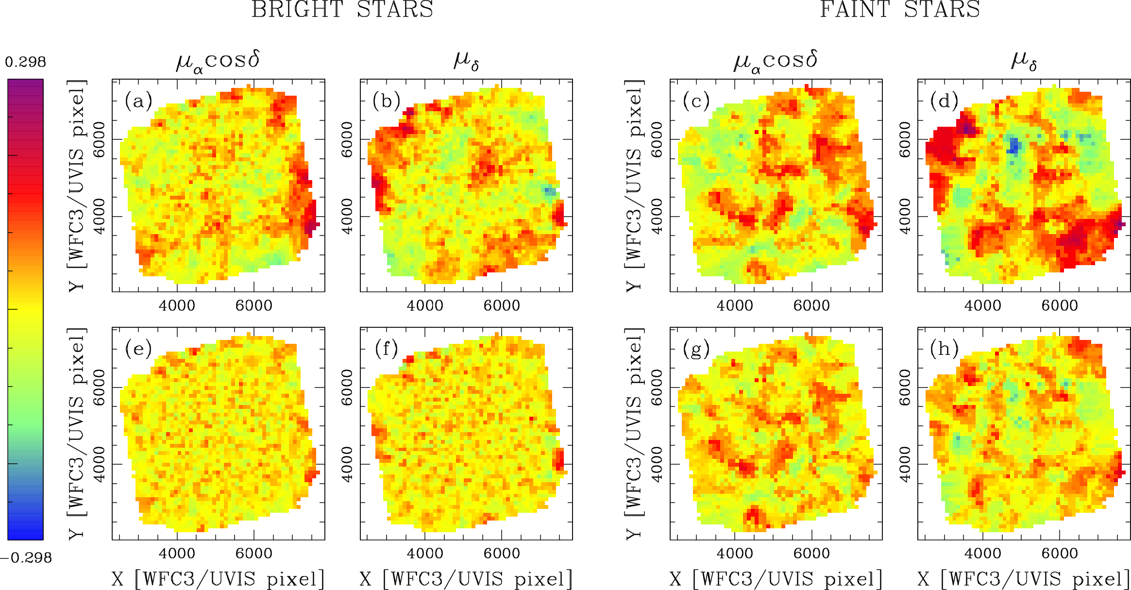
Figure 1: Local PM maps of NGC 5272 before (panels a, b, c, d) and after (panels e, f, g, h) the a-posteriori corrections. The four leftmost/rightmost panels are obtained using only stars brighter/fainter than the instrumental F606W magnitude of $-10$ (signal-to-noise ratio of $\sim$100; $m_{\rm F606W}\sim 21.6$). Points are color-coded according to the color bar on the left (in units of mas yr^-1). See the text for details.

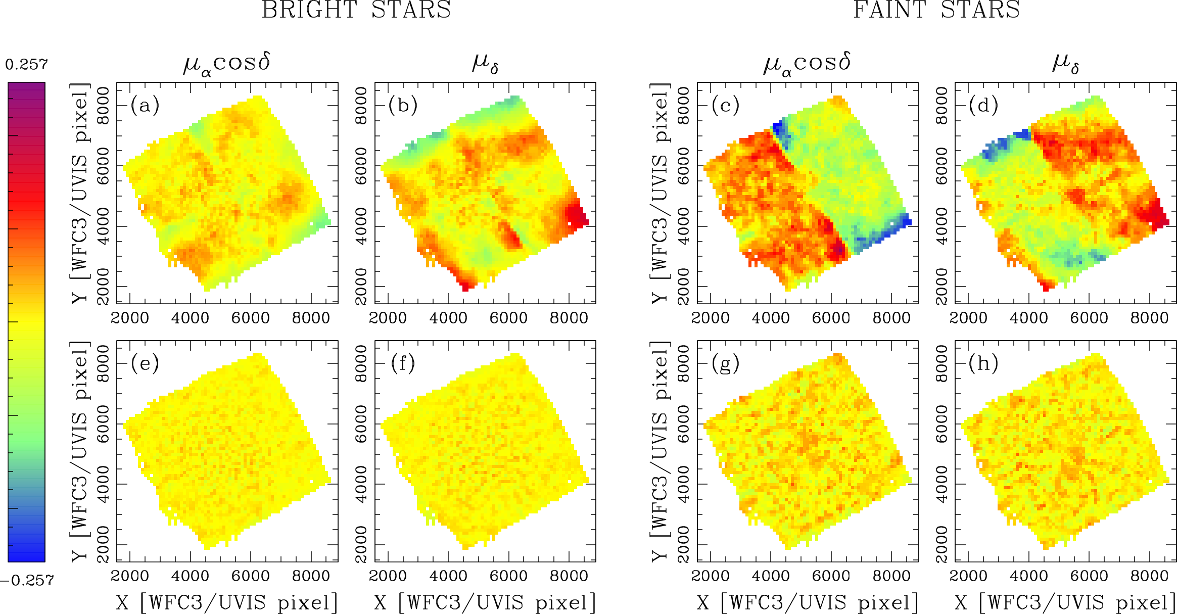
Figure 2: Similar to Fig. 1, but for the GC NGC 1261. The effects of residual, uncorrected CTE are clearly visible in panels (c) and (d).

3 Proper motions

PMs were computed following the procedures and caveats described in Bellini et al. (2014). Briefly, positions in the KS2-based raw catalogs were corrected for geometric distortion and then transformed (with six-parameter linear transformations) onto the same reference-frame system defined in Sect. 2. Only cameras/detectors/filters best suited for astrometry (see Bellini et al., 2014) were used in the PM computation. Then, the positions as a function of time were fit with a least-squares straight line. The slope of this straight line provides a direct estimate of the PM of the source. The PM errors are the uncertainties of the PM fit obtained by using the actual residuals of the points about the fitted line (Bellini et al., 2014).

For each source, the six-parameter linear transformations used in the PM computation were obtained by using a set of close-by, bright, well-measured cluster stars. Thus, our PMs are computed relative to the bulk motion of each GC at that given specific location in the FoV, and the cluster PM distribution is centered on the origin of the vector-point diagram (VPD). In addition, we also provide the PM zero-point needed to transform these relative PMs on to an absolute reference system (Appendix A).

Another important feature of our PM derivation is that any signature of internal cluster rotation in the plane of the sky is removed from the cluster stars, but it is present, with the opposite sign, in all other sources (Bellini et al., 2017b). Thus, we cannot directly infer cluster rotation from the kinematics of the cluster members. The same argument is also valid for the parallax effect (e.g. Libralato et al., 2018a, b).

Small spatially-variable and magnitude-dependent systematic errors are present in our uncorrected PMs. As in Bellini et al. (2018), we notice two main types of systematic errors:

• a low-frequency effect correlated with the temporal baseline, as well as number and types of images, used to compute the PMs. To remove this time-dependent systematic, we divided our sample in $N$ sub-groups based on the PM temporal baseline. $N$ varies from cluster to cluster due to the heterogeneous data sets used. Then, we computed the median PM of each sub-group, which should be zero by construction. If it was not zero, we subtracted this median PM value to the PM of each star in the sub-group;

• a high-frequency, spatially- and magnitude-dependent systematic error. By construction, the average PM of cluster stars should be zero regardless their magnitude and location in the field. This is not always true locally, mainly because of a combination of CTE and geometric-distortion residuals. These residual systematic errors were corrected using the median PM of the closest, both spatially and in magnitude, $N$ well-measured cluster members (target star excluded). The closeness criterion and the number of reference stars $N$ were tailored to each cluster to reach the best compromise between mapping the variations as locally as possible and the need for large statistics. For very-bright(faint) objects, we set up a magnitude threshold above(below) which reference stars are used for the correction instead of a fixed $\Delta$mag. This was done to increase the statistics at the extreme ends of the magnitude range.

The errors that we report in our catalogs for the PMs thus corrected include the propagated contributions from the uncertainties in the corrections themselves. When no enough reference stars were available for the high-frequency correction, this correction was not applied.

Figure 1 shows maps of raw and a-posteriori, locally-corrected PMs for the GC NGC 5272. The FoV has been divided into square cells of 100 WFC3/UVIS pixels per side. In each cell, we selected the 50 well-measured, cluster stars closest to the center of the cell, and computed the average PM in each direction. Panels (a) to (d) present the local PM maps obtained by means of the raw, uncorrected PMs, while panels (e) to (h) show the corrected PM maps. In each row, the two leftmost panels refer to stars brighter than the F606W instrumental magnitude equal to $-10$ (signal-to-noise ratio of $\sim$100; $m_{\rm F606W}\sim 21.6$), while the maps for fainter stars are shown in the two rightmost panels. The comparison between the top and bottom panels clearly highlights the effectiveness of the a-posteriori corrections. However, some residual high-frequency systematic errors are still present among the faintest objects. Thus, caution is advised when using these objects.

The raw PMs of some clusters, mainly those including the ACS/WFC data of the GO-14235 program (PI: Sohn), present larger systematics related to uncorrected CTE. The CTE that affects the HST detectors has worsened over time, and the official pipeline is not always able to completely correct it. An example is shown for NGC 1261 in the top panels of Figure 2, where it is clear that (i) bright and faint stars have different systematic errors in the PMs, and (ii) the local PM map of faint stars presents a discontinuity in the FoV along the chip gap of the GO-14235 data set. For these specific cases, we applied an additional a-posteriori correction prior to that for high-frequency systematics. Briefly, we divided our sample of well-measured stars into four magnitude bins. In each sub-sample, we computed the average PM (in each direction) of cluster members in 125-pixel-wide bins along the direction perpendicular to that of the CTE systematic on the local PM map. The corrections to the PM of each star were computed by interpolating among these binned values. As for the other a-posteriori corrections, the errors of this CTE-related correction are included in the corrected-PM error budget.

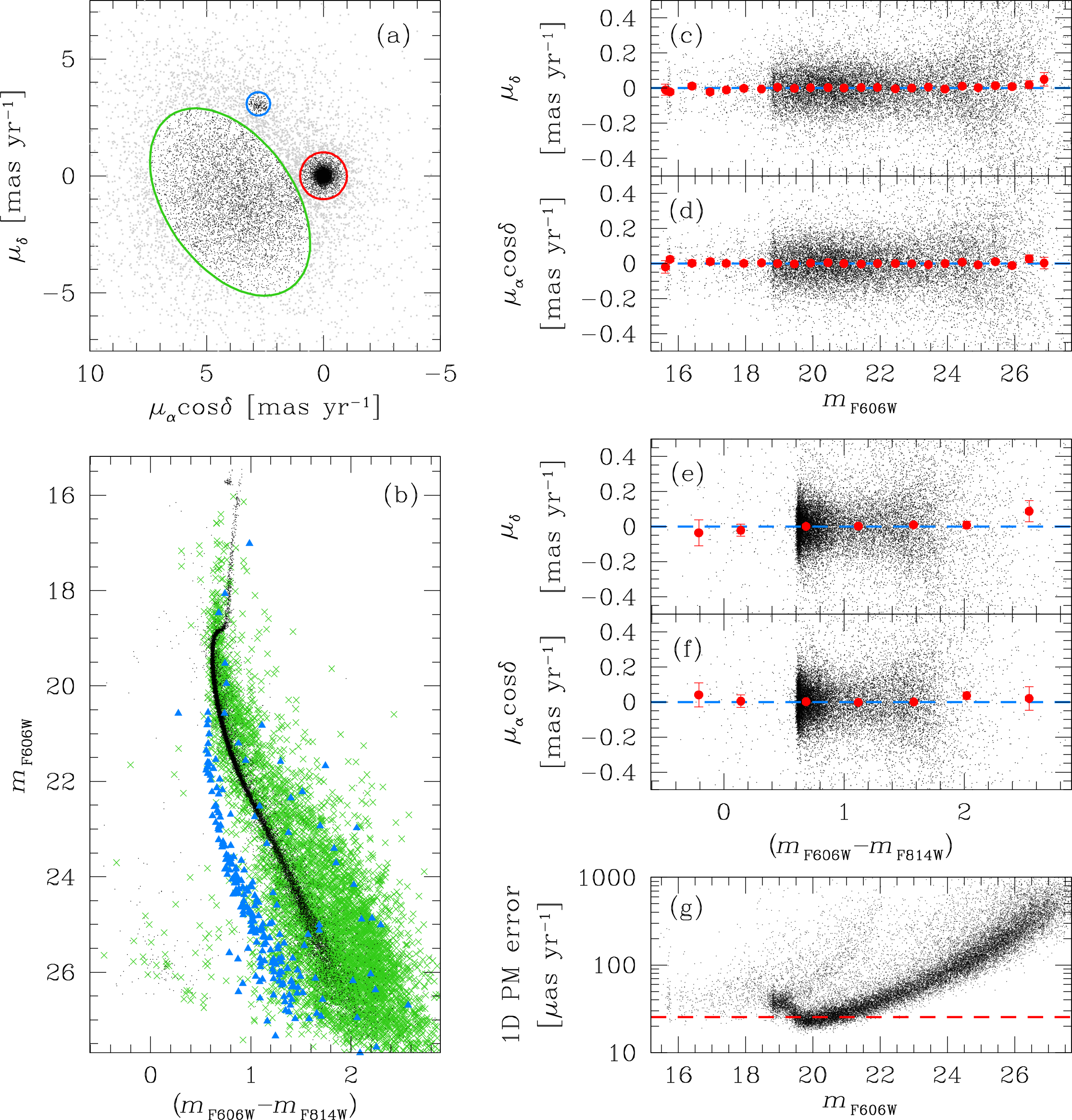
Figure 3: Overview of the PM catalog of NGC 6652. (a): VPD of the relative, corrected PMs. Stars within the red circle (centered on the origin of the VPD, and with radius of 1 mas yr^-1) are likely cluster members, the blue circle marks the location of Sagittarius-Dwarf objects, while the green ellipse highlights a group of Bulge stars. Gray dots are all sources outside any of these three selections (likely Bulge objects or cluster stars with large PM uncertainties). (b): $m_{\rm F606W}$ versus $(m_{\rm F606W}-m_{\rm F814W})$ CMD. Black dots are likely cluster members; blue triangles are members of the Sagittarius Dwarf; green crosses are Bulge objects (gray points in the VPD are not shown for clarity). (c) and (d): $\mu_{\delta}$ and $\mu_{\alpha}\cos\delta$ PMs as a function of $m_{\rm F606W}$. Only stars member of NGC 6652 are shown (black points). The red points (with error bars) are the median values of the PMs in 0.5-mag bins. The azure line is set to zero. (e) and (f): $\mu_{\delta}$ and $\mu_{\alpha}\cos\delta$ PMs as a function of $(m_{\rm F606W}-m_{\rm F814W})$. Panels (c) to (f) show no obvious trends of our corrected PMs with stellar magnitude and color. (g) 1D corrected-PM error (the sum in quadrature of the PM errors in each direction divided by $\sqrt{2}$) as a function of $m_{\rm F606W}$. The red line is set at the median value of the 1D PM errors of bright, well-measured unsaturated stars.

The steps described above generally remove the majority of systematic errors included in the raw PMs. However, these corrections are not perfect, especially for very faint stars, and we advise users to carefully check PMs for magnitude/color/spatial systematics on a cluster-by-cluster basis.

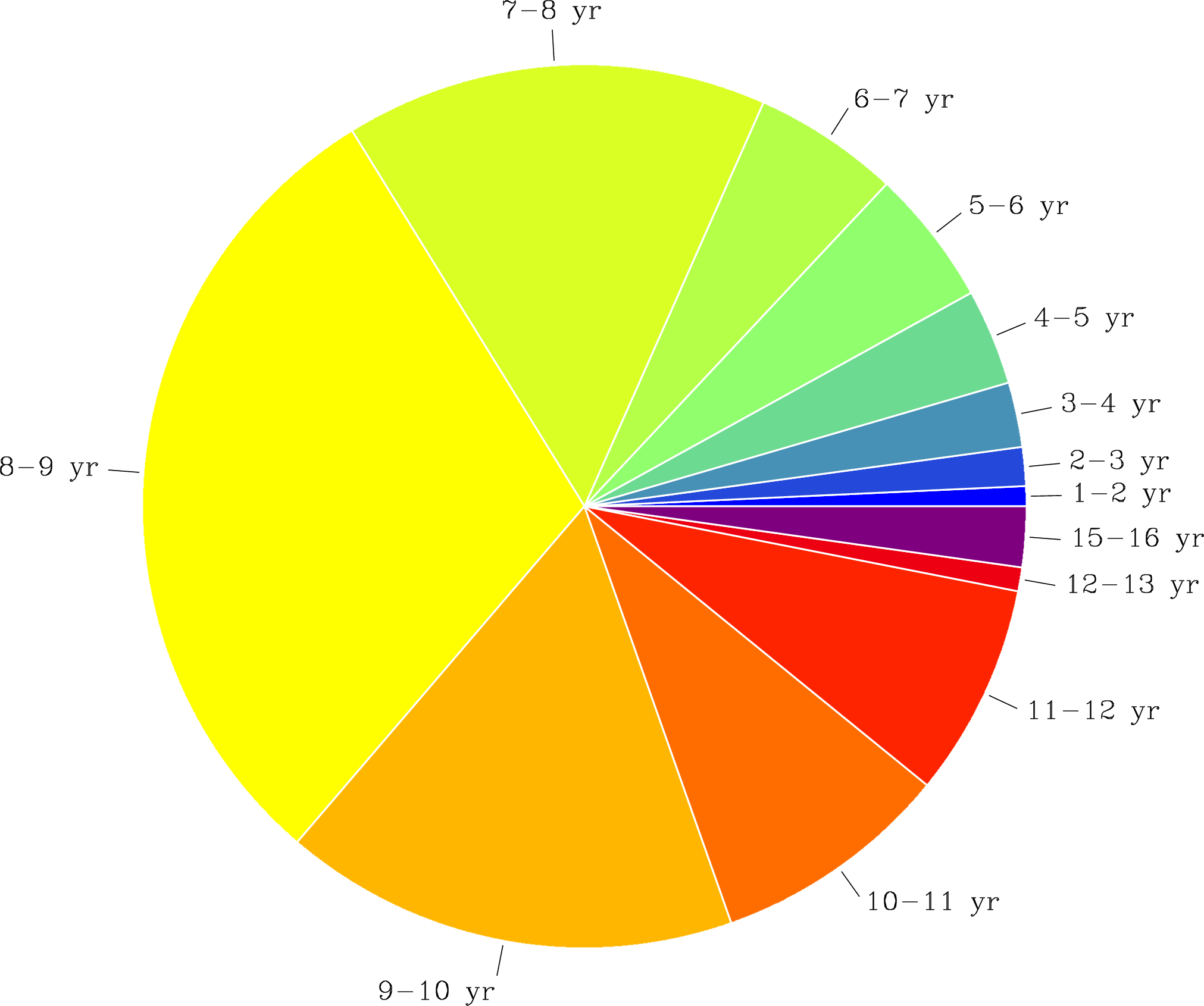
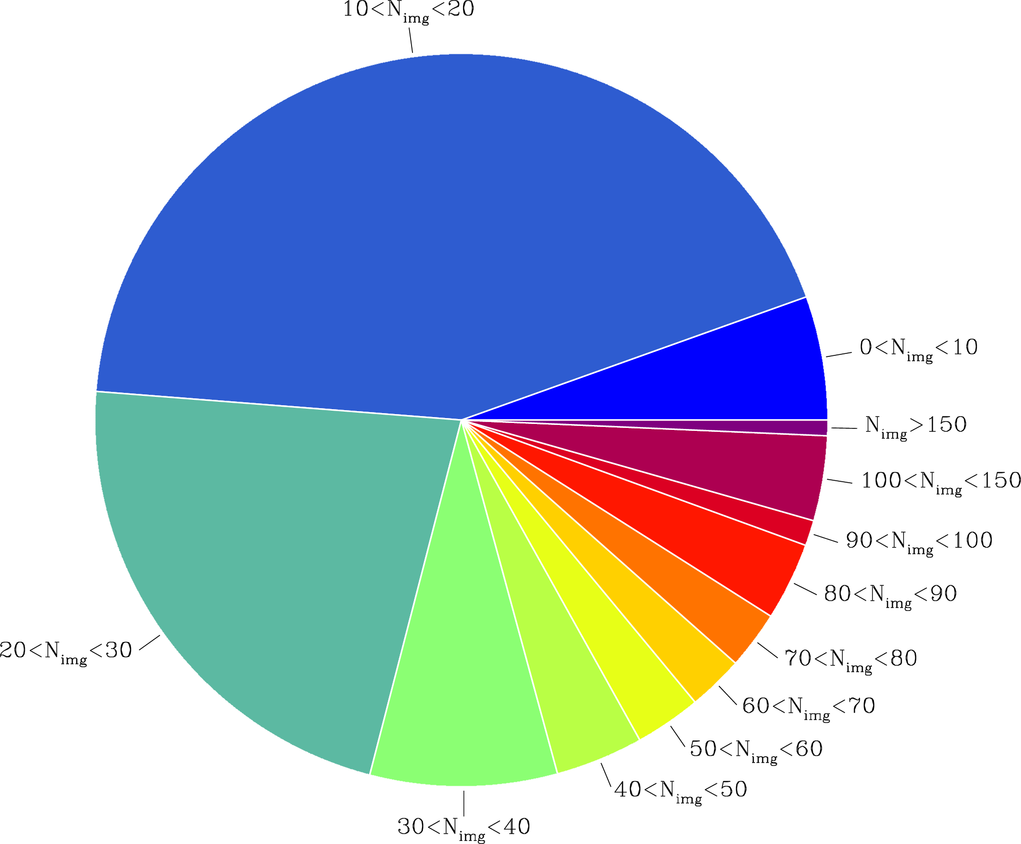
Figure 4: Pie charts of the total temporal baselines (left) and number of images used to compute PMs (right) in our catalogs.

Figure 3 provides an overview of the PM catalog of NGC 6652. This GC is located in the outer Bulge, projected on the Baade’s Window (Rossi et al., 2015), and in foreground of the Sagittarius Dwarf spheroidal. The VPD obtained with our corrected PMs is presented in panel (a). On the basis of their locations in the VPD, we arbitrarily define three groups of objects: cluster stars (points within the red circle), Sagittarius-Dwarf members (points within the blue circle), and Bulge stars (objects within the green ellipse). In the CMD in panel (b), we highlight members of NGC 6652 in black (stars within the red circle in the VPD), Bulge objects in green and stars associated with the Sagittarius Dwarf in azure. This is a simple example of one of the possible applications of our PM catalogs. Corrected PMs in each coordinate as a function of $m_{\rm F606W}$ are plotted in panels (c) and (d), and as a function of $(m_{\rm F606W}-m_{\rm F814W})$ color in panels (e) and (f). Only cluster members are shown. The red points (with error bars) are the median values of the PMs in 0.5-mag bins. The azure line is set to zero. These plots do not show any significant magnitude- or color-dependent systematics in our corrected PMs, but very blue and red objects hint at the presence of some residual color-dependent systematics. However, stars with these extreme colors are very faint (see panel b), and we expect both PMs and their corrections still to be affected by small systematic residuals. We stress, though, that no quality selections other than the membership were applied here. Finally, panel (g) shows the 1D corrected-PM error as a function of $m_{\rm F606W}$. The red, horizontal line is set at the median 1D PM error of bright, well-measured stars, i.e., 25.6 $\mu$as yr^-1.

A description of the final PM and photometric catalogs (together with some caveats about their usage) is provided in Appendix B, Tables A2 and A3, respectively. The precision of our PMs varies from cluster to cluster and depends on temporal baseline, as well as on the number and depth of images. Figure 4 presents pie charts of the temporal baselines and the number of images used to compute PMs in all our catalogs, respectively. About $\sim$33% of the PMs are computed with only 10–20 images and a temporal baseline between 7 and 9 yr, i.e., by combining only GO-10775 and GO-13297 data. The remaining PMs result from the mix of heterogeneous data sets. For bright, well-measured stars, the median raw-PM precision is between about 7 and 60 $\mu$as yr^-1, while that of corrected PMs ranges between about 13 and 120 $\mu$as yr^-1.

4 Internal kinematics of stellar clusters

As a benchmark for our PM catalogs, we here provide velocity-dispersion and anisotropy radial profiles of the clusters in our project. The kinematic profiles of the cores complement those in the outskirts derived with the Gaia Early Data Release 3 (EDR3) catalog (e.g., Vasiliev & Baumgardt, 2021). We also include the kinematic profile of the open cluster NGC 6791.

We started by selecting well-measured objects in each epoch/filter/camera combination as follows (see Table A3 for the explanation of the parameters):

1. magnitude rms lower than the 90-th percentile of the distribution at any given magnitude. An object with a magnitude rms better than 0.01 mag is always included in the well-measured sample, while all sources with a magnitude rms larger than 0.15 mag are excluded.

2. QFIT value larger than the 90-th percentile of the distribution at any given magnitude (note that the closer to 1 the QFIT parameter is, the better the PSF fit). Again, we retained all objects with a QFIT larger than 0.99 and discarded those with a value lower than 0.75.

3. $|$RADXS$|$ value lower than the 90-th percentile of the distribution at any given magnitude, but keeping all objects with a $|$RADXS$|$ lower than 0.01 and rejecting those with a value larger than 0.15;

4. the photometric $N_{\rm u}^{\rm phot}/N_{\rm f}^{\rm phot}$ ratio (see Table A3) is greater than 0.75;

5. $o<1$;

6. flux at least 3.5$\sigma$ above the local sky.

These (empirically-derived) thresholds were chosen as a compromise between rejecting bad measurements and keeping a large sample of stars for the subsequent analyses. To avoid crowding bias, we measured the 90-th-percentile trends for magnitude rms, QFIT and RADXS in a region outside the core of each cluster where sources are more isolated and applied these cuts to all stars across the FoV. When not enough stars were available outside the core of the cluster (for example, for the photometry obtained with ACS/HRC full-frame or WFC3/UVIS subarray images), all stars were used, regardless of their location in the FoV.

For each epoch, all criteria from (i) to (vi) have to be fulfilled in at least two filters if a star has been measured in at least two filters, otherwise in the only filter through which it was been detected. Finally, an object that has passed all previous selections is defined as “well-measured” if it passes all criteria in at least two epochs.

The PMs also provide useful parameters for selecting trustworthy sources for the kinematic analysis. In addition to all the previous criteria, we also removed all objects that have an astrometric $N_{\rm u}^{\rm PM}/N_{\rm f}^{\rm PM}$ ratio (see Table A2) smaller than 0.8–0.9 (the exact value changes from cluster to cluster), $\chi^{2}_{\mu_{\alpha}\cos\delta}$ and $\chi^{2}_{\mu_{\delta}}$ larger than 1.25–1.5, PM error larger than 0.5 mas yr^-1, or for which the a-posteriori PM correction was not computed. Finally, we also excluded stars with a PM error larger than $f$ times the local velocity dispersion $\sigma_{\mu}$ of a sub-sample of well-measured, close-by cluster stars. For each cluster, we compared the velocity-dispersion radial profiles of RGB stars obtained by varying $f$ from 0.5 to 0.9, with steps of 0.1, finding a general good agreement (within 1$\sigma$) between the inferred kinematics. If enough stars were left after all our quality selections, we used $f=0.5$. For 9 GCs (NGC 5053, NGC 5466, NGC 5897, NGC 6144, NGC 6366, NGC 6496, NGC 6535, NGC 6584 and NGC 6717), we used a value of $f=0.8$, while for NGC 6981 we set $f=0.9$. We included these 10 clusters in our analysis, but because their PM errors are of the order of their $\sigma_{\mu}$, we advise caution in the interpretation of their velocity-dispersion profiles.

All these criteria are designed to obtain a good compromise between statistics, quality and completeness. The only two exceptions to the strategy described above are NGC 362 and NGC 6352, for which we adopted the quality selections described in Libralato et al. (2018a) and Libralato et al. (2019), respectively.

GCs are old, collisional systems that, after many two-body relaxation times, present a (partial) degree of energy equipartition. Because of the heterogeneous mass ranges covered by our PM catalogs, we restricted the analysis of the kinematic profiles to stars brighter than the MS turnoff along the sub-giant and red-giant branches (SGB and RGB, respectively). Since in the post-MS evolutionary stages the evolutionary lifetimes are quite shorter than the core H-burning one, and in any case shorter than the typical two-body relaxation time, SGB and RGB stars can be safely considered as having the same kinematic mass (see also Sect. 6.3).

The velocity-dispersion profile of each cluster was obtained by dividing the sample of massive cluster members into equally-populated radial bins, with at least 100 stars per bin. In case of low statistics, we lowered the number of stars per bin to ensure at least 3 radial bins, regardless of the number of stars within each bin. When the statistics allowed, we also imposed a radial bin comprising only the centermost 5–10 arcsec. The velocity dispersion in each radial bin was computed similarly to what is described in Raso et al. (2020), i.e., by maximizing the following likelihood:

$$\ln\mathcal{L}=-\frac{1}{2}\sum_{n}\Bigl{[} \frac{(v_{\rm rad,\,n}-v_{\rm rad})^{2}}{\sigma_{\rm rad}^{2}+\epsilon_{\rm rad,\,n}^{2}}+\ln(\sigma_{\rm rad}^{2}+\epsilon_{\rm rad,\,n}^{2})+$$ (1)

$$\frac{(v_{\rm tan,\,n}-v_{\rm tan})^{2}}{\sigma_{\rm tan}^{2}+\epsilon_{\rm tan,\,n}^{2}}+\ln(\sigma_{\rm tan}^{2}+\epsilon_{\rm tan,\,n}^{2})\Bigr{]}\mathrm{,}$$

where $(v_{\rm rad,\,n},v_{\rm tan,\,n})$ are the radial and tangential components of the PM of the $n$-th star, $(\epsilon_{\rm rad,\,n},\epsilon_{\rm tan,\,n})$ are the radial and tangential components of the PM uncertainty of the $n$-th star, $(v_{\rm rad},v_{\rm tan})$ are the radial and tangential mean motions of the cluster, and $(\sigma_{\rm rad},\sigma_{\rm tan})$ are the radial and tangential velocity dispersions of the cluster. We also computed the combined velocity dispersion $\sigma_{\mu}$ in each radial bin using the same likelihood in Eq. 1 but with $\sigma_{\rm rad}=\sigma_{\rm tan}=\sigma_{\mu}$. We used the affine-invariant Markov Chain Monte Carlo (MCMC) method emcee (Foreman-Mackey et al., 2013) to sample the parameter space and obtain the posterior probability distribution functions (PDFs) for $\sigma_{\mu}$, $\sigma_{\rm rad}$ and $\sigma_{\rm tan}$. We run the MCMC chain with 20 walkers for 5000 steps, then rejected the first 200 steps. The best-fit values correspond to the medians of the PDFs, while the corresponding errors are defined as the average between the 16-th and 84-th percentile about the median. Finally, the velocity dispersions were corrected as described in Watkins et al. (2015a, but see also Appendix A of ) to take into account the maximum-likelihood estimators being biased and underestimating the true dispersion of the velocity distribution. The difference between the corrected and uncorrected $\sigma_{\mu}$ is, on average, $\sim$0.6%, it never reaches 3% and it is more important for bins with fewer than 100 stars.

Figures A2–A5 in Appendix C show the result of our analysis for the 57 stellar clusters in the GO-13297 project. These profiles are also available at our website. For each cluster, the $m_{\rm F606W}$ versus $(m_{\rm F606W}-m_{\rm F814W})$ CMD is shown on the rightmost panel. Well-measured members of the GC brighter than the MS turnoff (highlighted by the azure, dashed horizontal line) are plotted as red points, all other objects that passed the quality criteria are shown as black points.

Table 1: Gaia-based velocity dispersions for NGC 6791.

Radius	$\sigma_{\mu}$
$[$arcsec$]$	$[$mas yr-1$]$
73.55	$0.096\pm 0.005$
144.58	$0.074\pm 0.005$
222.38	$0.075\pm 0.005$
311.43	$0.075\pm 0.005$
487.58	$0.066\pm 0.005$

The velocity dispersion $\sigma_{\mu}$ as a function of distance from the center of the cluster is presented in the bottom-left panel. Black, filled points are obtained from this work, while black, open points refer to the measurements in the GC database of Holger Baumgardt obtained with the Gaia EDR3 PMs, which were presented by Vasiliev & Baumgardt (2021). The only exception is NGC 6791, which is not included in the work of Vasiliev & Baumgardt (2021). For this cluster, we independently derived Gaia-based $\sigma_{\mu}$ using our tools (Table 1). The black dashed lines are set at the core ($r_{\rm c}$; obtained using the definition in Spitzer 1987, see Eq. 1-34, which is similar to the definition of the King scale radius $r_{0}$) and the projected half-light ($r_{\rm h}$) radii provided in the Baumgardt’s database. For NGC 6791, we used $r_{\rm c}$ and $r_{\rm h}$ from Dalessandro et al. (2015) and Kamann et al. (2019), respectively.

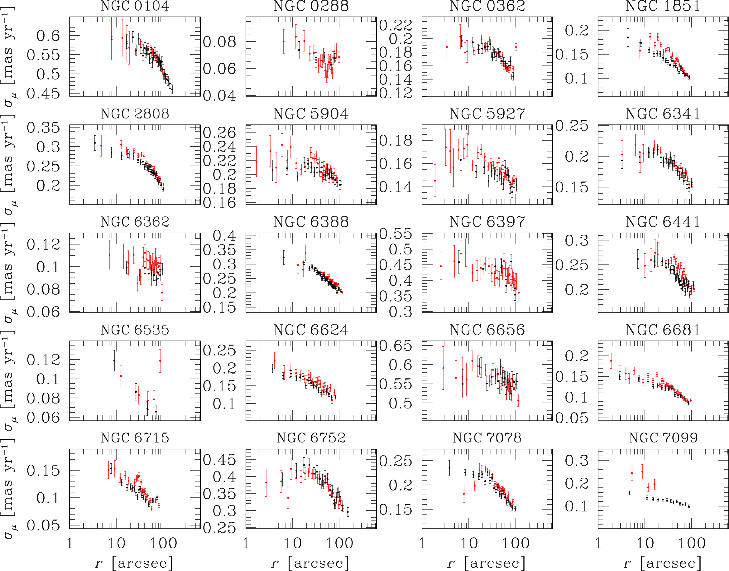
Figure 5: Comparison of the velocity-dispersion radial profiles obtained with HST-based PMs in this paper (black points) and in Watkins et al. (2015a, red points).

Vasiliev & Baumgardt (2021) used all stars at their disposal regardless of their magnitude. Thus, the Gaia-based velocity dispersions for close-by clusters were derived from stars with various masses and, because of the effects of energy equipartition, could be systematically higher than our HST-based profiles. However, Vasiliev & Baumgardt (2021) argued that the Gaia uncertainties for faint stars are likely underestimated, and included a scaling factor for the PM errors to obtain consistent $\sigma_{\mu}$ values between different magnitude intervals. Furthermore, the authors applied various quality cuts to their samples prior to the determination of the PM velocity dispersions (see their Sect. 3), which likely excluded from the fits faint (and so low-mass) objects with large PM uncertainties. For this reason, we choose to directly compare our HST profiles in the cores with these Gaia velocity dispersions outside the cores. Overall, we find a good agreement between HST and Gaia profiles, with a few exceptions. NGC 5466 and NGC 6981 have HST PM uncertainties of the same order of the $\sigma_{\mu}$ (we used a large value of $f$ for the analysis), thus the inferred values of $\sigma_{\mu}$ should be interpreted cautiously. For NGC 6934, most of the Gaia stars used by Vasiliev & Baumgardt (2021) have PM errors larger than the intrinsic $\sigma_{\mu}$ of the cluster, and the Gaia measurements might not be completely reliable. The HST profile of NGC 6304 seems higher than the one from the Gaia PMs. However, the HST-based kinematics are in agreement with the line-of-sight (LOS) velocities in the Baumgardt’s database.

We fit these points with a 4-th order monotonically-decreasing polynomial. The coefficients of the 4-th-order polynomial are obtained with a maximum-likelihood approach. For each cluster in Figures A2–A5, the blue line in the bottom-left panel is obtained with the best-fit (median) values of the polynomial fit, while the cyan lines are 100 random solutions of the polynomial fit. We used these polynomial functions to derive the $\sigma_{\mu}$ at the center of each cluster, at $r_{\rm c}$ and at $r_{\rm h}$. We provide all these values in Table A4.

The polynomial fits show again the agreement between HST and Gaia data for most of the clusters. There are a few points that are outliers with respect to the polynomial-fit predictions. Most of these outliers refer to the velocity dispersion in the innermost bins. A rise of the velocity dispersion in the innermost region can be a proxy for the presence of an intermediate-mass black hole (Greene et al., 2020, and references therein), but also for issues related to crowding/blending. Indeed, if two sources are blended and confused as one, or if the light contamination from the neighbors is high (which can still occour even with our data reduction), the position measured can be shifted from the real position. The offset is different for every image/filter/camera. Hence, the net result is that its PM is likely larger than what it should be, thus increasing the $\sigma_{\mu}$ of the sources in the very-crowded region (see the discussion in Bellini et al., 2014). Finally, the shape and the abrupt drop of the polynomial functions in the outermost parts of the FoV do not correspond to physical effects and are just plotted for completeness.

The anisotropy ($\sigma_{\rm tan}/\sigma_{\rm rad}$) as a function of distance from the center of the cluster is presented in the top-left panels. Anisotropy is discussed in Vasiliev & Baumgardt (2021), but their values are not publicly available. Thus, only HST-based data are shown in the top-left panels of Figs. A2–A5 (black, filled dots). The red, dashed, horizontal line is set to 1 and marks the isotropic case. Most clusters are isotropic in the core, but a few objects show a radial anisotropy outside about one $r_{\rm h}$. We will discuss the kinematic anisotropy in detail in the next Section.

Jindal et al. (2019) analyzed 10 GCs using Gaia DR2 data and made publicly available their velocity dispersion and anisotropy radial profiles. Although their profiles do not cover the centermost region observed by our HST data, we find an agreement at the 1$\sigma$ level between their $\sigma_{\mu}$ and anisotropy values for the nine clusters in common with our data set.

We also compared our kinematic profiles with those of Watkins et al. (2015a), see Fig. 5, where a previous version of the HST PM catalogs was used (Bellini et al., 2014). There is an overall agreement between the profiles at the 3$\sigma$ level. The profiles of Watkins et al. (2015a) for NGC 1851, NGC 6441 and NGC 7078 are generally higher than those in our work. For NGC 7078, we also do not see the drop of the velocity dispersion in the centermost region as seen by Watkins et al. (2015a). A similar discrepancy is found when comparing the profiles of NGC 2808, NGC 6681 and NGC 6715, although at to lesser extent. The reason for these discrepancies might be the better treatment of crowding in our data reduction and/or the additional quality selections applied in our work. The profile of NGC 7099 is instead completely different, but the PMs used by Watkins et al. (2015a) were computed with a temporal baseline of only two years (see Bellini et al., 2014), and their quality is worse than that of our PMs.

The velocity-dispersion profile of NGC 6441 was also studied by Häberle et al. (2021). The PMs computed by Häberle et al. (2021) are obtained from a combination of data taken with ACS/HRC@HST and NACO@VLT detectors, which are better suited for probing the centermost arcsec of this very-crowded cluster. Our PM profile seems to suggest a more moderate increase of the velocity dispersion toward the center, although the values in the region in common within 10 arcsec from the center are in agreement at the 1$\sigma$ level. The central velocity dispersion inferred in our work with the polynomial fit is $\sigma_{\mu}^{r=0}=(0.285\pm 0.012)$ mas yr^-1, while their $\sigma_{\mu}$ measured at $r\sim 0.76$ arcsec is $(0.316\pm 0.034)$ mas yr^-1. It is hard to clarify the nature of the discrepancy between these profiles given the different resolutions of the instruments used to infer the PMs in the centermost arcsec of the cluster.

Finally, we compared our PM velocity dispersions with those based on LOS velocities in the Baumgardt database, which are taken from various sources in the literature. There is an overall agreement between the PM- and LOS-velocity-based profiles, although there are discrepancies in some cases (NGC 5053, NGC 5272, NGC 5286, NGC 5466, NGC 6093, NGC 6101, NGC 6144, NGC 6205, NGC 6584, NGC 6681, NGC 6809, NGC 6981 and NGC 7099) where our PM-based $\sigma_{\mu}$ are higher than the $\sigma_{\rm LOS}$, either in general or only in the centermost bins. The origin of the differences between PM- and LOS-velocity-based profiles might be related to systematics in either data sets, errors in the cluster distance (see Sect. 5.1), or instead be a proxy of a peculiar kinematic state of the cluster. However, a detailed comparison between these $\sigma_{\mu}$ is outside the scope of this paper.

5 General kinematic properties

The collection of kinematic profiles in Figures A2–A5 allows us to analyze some of the general properties of stellar clusters, similar to what has already been done in the literature (e.g., Watkins et al., 2015a), but with a larger sample. We cross-correlated the kinematic pieces of information derived by means of HST and Gaia data with the structural properties of the GCs.

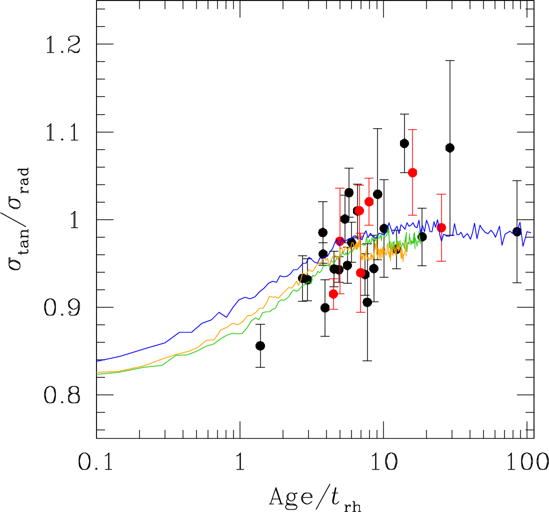
Figure 6: Anisotropy at the half-light radius as a function of the ratio of the cluster age to the half-mass relaxation time. An isotropic system is characterized by $\sigma_{\rm tan}/\sigma_{\rm rad}=1$. Red points refer to core-collapsed GCs. All other systems are shown as black dots. The three solid lines show the time evolution of $\sigma_{\rm tan}/\sigma_{\rm rad}$ from three Monte Carlo simulations with initial $W_{0}$ and filling factors (defined as the ratio of the half-mass to tidal radius) equal to (5, 0.09; green line), (5, 0.18; blue line), (7, 0.06; orange line); the three systems reach core collapse, respectively, at Age$/t_{\rm rh}\simeq$ 10.9, 24.7, 6.8.

A quantity of particular interest in the kinematic characterization of star clusters is the anisotropy of the velocity distribution. Simulations following the evolution of star clusters during the initial violent-relaxation phase and including the effects of the tidal field of the host galaxy have shown that these systems emerge from this early evolutionary phase with an isotropic velocity distribution in the core, a radially anisotropic distribution in the intermediate regions, and an isotropic or slightly tangentially anisotropic distribution in the outermost regions (see Vesperini et al., 2014). This specific configuration depends on the initial conditions at the formation of the cluster, on the surrounding environment, and it changes during the subsequent long-term evolution; in particular during a cluster’s long-term evolution, the effects of two-body relaxation and mass loss lead to a gradual decrease of the radial anisotropy imprinted during the early dynamical phases (Tiongco et al., 2016b, see that paper also for the possible development of radial anisotropy in tidally underfilling clusters with an initial isotropic velocity distribution).

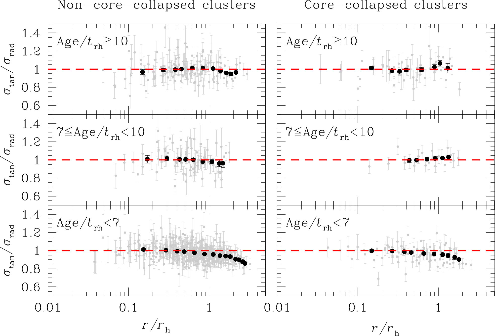
Figure 7: Anisotropy as function of distance from the center of the cluster in units of $r_{\rm h}$. The red, dashed, horizontal line is set at 1. Gray dots refer to the individual measurements shown in Figs. A2–A5. Black points, with error bars, are the 3.5$\sigma$-clipped average values of the the anisotropy in 1-$r_{\rm h}$-wide bins (steps of 0.25 $r_{\rm h}$; only bins with at least 5 points are considered). From top to bottom, the plots refer to clusters with Age/$t_{\rm rh}\geq 10$, $7\leq$ Age/$t_{\rm rh}<10$ and Age/$t_{\rm rh}<7$. Left panels refer to non-core-collapsed clusters, while those on the right shows the results for core-collapsed clusters.

Figure 6 shows the ratio between the tangential and radial components of the velocity dispersions measured at the half-light radius as a function of the dynamical ages of the clusters as measured by the ratio of their physical age to their half-mass relaxation time ($t_{r{\rm h}}$; from the Baumgardt catalog). The values of $\sigma_{\rm tan}$ and $\sigma_{\rm rad}$ at the half-light radius were derived by fitting a 4-th order polynomial function to the corresponding profile as described in Sect. 4. We excluded from the plot all GCs for which the HST data do not reach the half-light radius (so the anisotropy ratio would need to be extrapolated). Red points represent core-collapsed GCs, while all other systems are presented as black points. Core-collapsed GCs (regardless of whether they are considered as ‘possible’ or ‘post’ core-collapsed GCs) were labeled as such according to Trager et al. (1995) or, if they were not included in that list, according to the Harris catalog. Our analysis shows that dynamically older clusters (Age/$t_{\rm rh}$ $\gtrsim$ 10) tend to be isotropic even at the half-light radius, while dynamically-young systems are characterized by a radially-anisotropic velocity distribution at the half-light radius. A transition between the two regimes happens at Age/$t_{\rm rh}$ between 7 and 10. These findings are consistent with the theoretical expectations discussed above (see, e.g., Vesperini et al., 2014; Tiongco et al., 2016b; Bianchini et al., 2017) and previous observational works (Watkins et al., 2015a).

To further illustrate the theoretical expectations concerning the evolution of the radial anisotropy, in Fig. 6 we show the time evolution of $\sigma_{\rm tan}/\sigma_{\rm rad}$ (calculated at the projected half-light radius) from a few Monte Carlo simulations run with the MOCCA code (Giersz et al., 2013). The simulations follow the dynamical evolution of a few simple stellar systems composed of 500k stars with masses following a Kroupa (2001) initial mass function between 0.1 and 0.8 $M_{\odot}$, and spatially distributed according to the density profiles of King (1966) models with values of the central dimensionless potential equal to $W_{0}=5$ and $W_{0}=7$ (corresponding, respectively, to $c\simeq 1.03$ and $c\simeq 1.53$). The systems are characterized by an initial anisotropic velocity distribution following the Osipkov-Merrit profile (see, e.g., Binney & Tremaine, 2008), $\beta=1-\sigma_{\rm tan}^{2}/(2\sigma_{\rm rad}^{2})=1/(1+r_{\rm a}^{2}/r^{2})$ with $r_{\rm a}$ equal to the half-mass radius. As shown in this plot, the initial anisotropy of the clusters at the half-light radius gradually decreases during the cluster’s long-term evolution. For the tidally filling system, the enhanced rate of star loss leads to a more rapid isotropization of the velocity dispersion. At the time when the system reaches core collapse, the cluster’s radial anisotropy slightly increases, then continues its gradual decrease toward isotropy (see also Tiongco et al., 2016b, for a study of the evolution of anisotropy for systems with a variety of different initial conditions). The differences between the anisotropy of systems that have similar dynamical ages but are in the pre- or post-core-collapsed phase is small, and within the uncertainty of the observed values.

In Fig. 7, to further investigate the kinematic anisotropy in stellar clusters, we divided the sample into three groups, i.e., clusters with a Age/$t_{\rm rh}\geq 10$, between 7 and 10 (the Age/$t_{\rm rh}$ transition region found in Fig. 6), and lower than 7. In each group, we also separated core-collapsed clusters (right panels) from all other systems (left panels). We collected all anisotropy measurements shown in Figs. A2–A5, and plotted them as a function of distance from the center of the cluster in units of $r_{\rm h}$. Gray points are the individual measurements, while black dots are the moving averages of those points. Clusters with Age/$t_{\rm rh}\geq 10$ are isotropic at all distances within our FoV, regardless of their core-collapsed status, which is what we expected. Clusters with Age/$t_{\rm rh}$ between 7 and 10 are again shown to be isotropic at all distances, although the non-core-collapsed sample hints at a marginal radial anisotropy at $r\gtrsim r_{\rm h}$. Finally, dynamically-young clusters clearly present the expected radial anisotropy at large radii.

Thus, clusters that underwent a core collapse seem to have similar velocity fields as those of the other GCs with similar dynamical ages; this appears to be consistent with what suggested by the results of the simulations presented in Fig. 6, which show that core collapse has only a relatively small effect on the radial anisotropy measured at the half-light radius. Additional simulations and a larger observational sample of core-collapsed clusters are necessary to further explore this issue. In particular, it is worth noticing that the core-collapsed sample with Age/$t_{\rm rh}<7$ is composed of only four clusters: NGC 6541, NGC 6752, NGC 7099 and NGC 7078. While the first three objects show an isotropic field even slightly farther than the half-light radius, the latter presents a strong radial anisotropy. This feature for NGC 7078 has also been noted by Bellini et al. (2014) and Vasiliev & Baumgardt (2021). Among these four GCs, NGC 7078 (i) is more massive, (ii) is further from the center of the Galaxy, and (iii) has had fewer interactions with the Galactic potential of the Bulge/Bar and Disk (see Vasiliev & Baumgardt, 2021). The combination of these properties could have preserved some of the original radial anisotropy in the innermost regions (e.g., Vesperini et al., 2014).

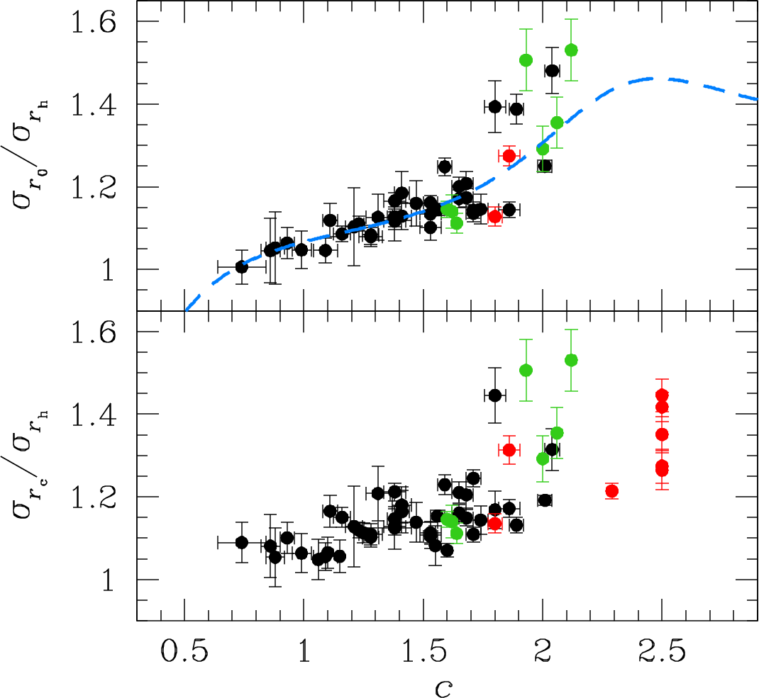
Figure 8: (Bottom panel): ratio between the velocity dispersion at the core and half-light radii (from the Baumgardt catalog) as a function of concentration index $c$. The values of $c$ are obtained from McLaughlin & van der Marel (2005). For GCs not analyzed in that work, we used the values from Harris (1996, 2010 edition). Red points are GCs that are marked as core-collapsed in the Harris catalog; green dots are measurements from Cohen et al. (2021); black dots are all other objects. (Top panel): as in the bottom panel, but using the velocity dispersion at $r_{0}$ and $r_{\rm h}$ (radii from McLaughlin & van der Marel, 2005). Some core-collapsed GCs are missing from the plot because they were not analyzed by McLaughlin & van der Marel (2005). The results obtained with the LIMEPY models are shown as an azure, dashed line.

Core-collapsed GCs are not only more spatially concentrated than other GCs, but their velocity-dispersion radial profiles are also steeper. This has been shown by Watkins et al. (2015a) and Cohen et al. (2021). In Fig. 8, we provide an updated version of this finding, and a comparison with theoretical models. The bottom panel of Fig. 8 shows the ratio between the velocity dispersion at the core and half-light radii ($\sigma_{r_{\rm c}}/\sigma_{r_{\rm h}}$), computed as described before at $r_{\rm c}$ and $r_{\rm h}$ from the Baumgardt catalog, as a function of the concentration index $c$. The values of $c$ are taken from McLaughlin & van der Marel (2005) and are defined as the $\log(r_{\rm t}/r_{0})$, where $r_{\rm t}$ and $r_{0}$ are the tidal and King scale radii, respectively. We selected $c$ as obtained from the fit of a King (1966) profile. If $c$ is not provided for a GC in the work of McLaughlin & van der Marel (2005), we used the value in Harris (1996, 2010 edition). Red, filled circles mark core-collapsed GCs, while all other systems are plotted as black dots. Green points are clusters taken from the sample of Cohen et al. (2021). This panel highlights a different location in the plot for core-collapsed GCs and the other stellar systems. This Figure confirms the trend between the spatial concentration and the steepness of the radial profile of the velocity dispersion.

In order to further explore this trend and carry out a consistent comparison with theoretical models, we show in the top panel of Fig. 8 the ratio of the values of the the velocity dispersions calculated at the King scale radius and at the half-light radius (this time obtained at $r_{0}$ and $r_{\rm h}$ of McLaughlin & van der Marel, 2005, for consistency) versus the concentration $c$ together with a line showing the expected variation of these quantities along the sequence of King models (calculated using the LIMEPY software; Gieles & Zocchi, 2015). The overall agreement between the observed and the theoretical sequences shown in the top panel of Fig. 8 further supports the idea that more concentrated GCs have a steeper velocity-dispersion radial profiles according to what is expected for the family of King models with different values of $c$. It is interesting to notice the increasing deviation of the observational data from the theoretical King sequence at larger concentrations ($c\gtrsim 1.6$), including some of those from the sample of Cohen et al. (2021, green points in Fig. 8), which, according to those authors, are in an advanced dynamical state, being close to (or having recently undergone) core collapse. Although this issue requires further investigation, it may represent a kinematic manifestation of the deviation of clusters from the dynamical properties of King models as they approach core-collapse.

There are a few exceptions in the overall picture described in the top panel of Fig. 8. The core-collapsed GC with $c<2.0$ and $\sigma_{r_{\rm c}}/\sigma_{r_{\rm h}}<1.2$ is NGC 362. NGC 362 is a post-core-collapsed GC (e.g., Dalessandro et al., 2013; Libralato et al., 2018a), and its peculiar position could be explained by the structural and dynamical evolution of post-core-collapsed GCs being driven by gravothermal oscillations (e.g., Makino, 1996).

Three clusters shown with black dots seem to have characteristics similar to core-collapsed GCs. These GCs are NGC 5272, NGC 6652 and NGC 6715. McLaughlin & van der Marel (2005) pointed out that NGC 5272 shows deviations from the classical King isotropic model, and can be better fit with other models (see also Da Costa & Freeman, 1976; Gunn & Griffin, 1979). NGC 6652 is not considered a core-collapsed GC, but it is very concentrated and has a very steep surface-brightness profile, typical of core-collapsed systems (Noyola & Gebhardt, 2006). NGC 6715 is a cluster at the center of the Sagittarius Dwarf, an environment that could explain its peculiar core-collapsed-like concentration.

5.1 Kinematic distances

The Baumgardt’s GC database also contains LOS velocity measurements. We made use of them to estimate distances of GCs by using the simple relation between the velocity dispersion along the LOS and in the plane of the sky:

$$\sigma_{\rm LOS}=4.7404\,d\,\sigma_{\mu}\,;$$ (2)

where $d$ is the distance in kpc, $\sigma_{\rm LOS}$ and $\sigma_{\mu}$ are the velocity dispersions along the LOS (in km s^-1) and in the plane of the sky (from PMs in mas yr^-1), respectively, and 4.7404 (km yr kpc^-1 mas^-1 s^-1) is the conversion factor. The only assumption here is that the GCs are isotropic. We computed the distance $d$ by comparing the values of the velocity dispersion at the same distance, i.e., at the center of the cluster, obtained for both LOS and PM measurements by fitting a polynomial function to the corresponding velocity-dispersion radial profiles as described in Sect. 4. Our results are summarized in Table 2. We considered only clusters with enough LOS velocities to solve the polynomial fit.

Figure 9 shows comparisons between our distances and those from Baumgardt & Vasiliev (2021, panel a; using Gaia parallaxes, the comparison between PM and LOS velocities, and/or star counts), the Harris catalog (panel b; collected from various sources in the literature), the work of Watkins et al. (2015b, panel c; obtained with an approach similar to that used in our paper) for a sample of 14 GCs, and the estimates from Recio-Blanco et al. (2005, panel d; using the luminosity level of the zero-age horizontal branch). The median differences between $d$ in our work and those in the literature shown in Fig. 9 are $(-0.01\pm 0.16)$ (Baumgardt & Vasiliev, 2021), $(-0.05\pm 0.18)$ kpc (Harris catalog), $(-0.19\pm 0.17)$ kpc (Watkins et al., 2015b), and $(-0.23\pm 0.20)$ kpc (Recio-Blanco et al., 2005), respectively. All distance estimates are in agreement with these literature values at the $\sim$1$\sigma$ level. This is further proof of the goodness of our PM measurements. At large distances ($>$10 kpc), the differences between our distances and those from the literature increase, and so does the scatter of the points in Fig. 9. The lower velocity dispersions of some of these clusters, as well as the larger uncertainties both in the PMs, LOS velocities and parallaxes, are likely the reasons for these discrepancies.

Table 2: GC kinematic distances.

Cluster	$d$	Cluster	$d$
	$[$kpc$]$		$[$kpc$]$
NGC 104	$4.34\pm 0.06$	NGC 6218	$5.23\pm 0.30$
NGC 288	$9.08\pm 0.79$	NGC 6254	$5.37\pm 0.21$
NGC 362	$9.33\pm 0.31$	NGC 6304	$7.50\pm 1.04$
NGC 1261	$13.14\pm 1.23$	NGC 6341	$7.68\pm 0.66$
NGC 1851	$11.66\pm 0.25$	NGC 6362	$9.02\pm 0.93$
NGC 2808	$10.07\pm 0.24$	NGC 6388	$11.69\pm 0.30$
NGC 3201	$4.73\pm 0.15$	NGC 6397	$2.25\pm 0.11$
NGC 4590	$10.44\pm 1.28$	NGC 6441	$13.15\pm 0.63$
NGC 4833	$7.21\pm 0.93$	NGC 6541	$7.36\pm 0.38$
NGC 5024	$14.86\pm 1.69$	NGC 6624	$7.91\pm 0.59$
NGC 5272	$8.16\pm 0.52$	NGC 6656	$3.03\pm 0.09$
NGC 5286	$9.65\pm 0.61$	NGC 6681	$11.10\pm 0.68$
NGC 5897	$15.35\pm 3.04$	NGC 6715	$25.32\pm 2.31$
NGC 5904	$7.42\pm 0.21$	NGC 6723	$7.65\pm 0.81$
NGC 5927	$9.33\pm 0.75$	NGC 6752	$3.85\pm 0.13$
NGC 5986	$10.61\pm 1.28$	NGC 6809	$4.62\pm 0.37$
NGC 6093	$9.34\pm 0.41$	NGC 7078	$10.81\pm 0.21$
NGC 6121	$1.85\pm 0.10$	NGC 7089	$10.36\pm 0.33$
NGC 6171	$6.36\pm 0.54$	NGC 7099	$9.50\pm 0.32$
NGC 6205	$6.16\pm 0.44$

6 Possible applications

We choose the GC NGC 5904 to showcase some scientific applications enabled by our PMs. Note that not all PM catalogs provide the same PM precision and overall quality, and some of the examples described below cannot be applied.

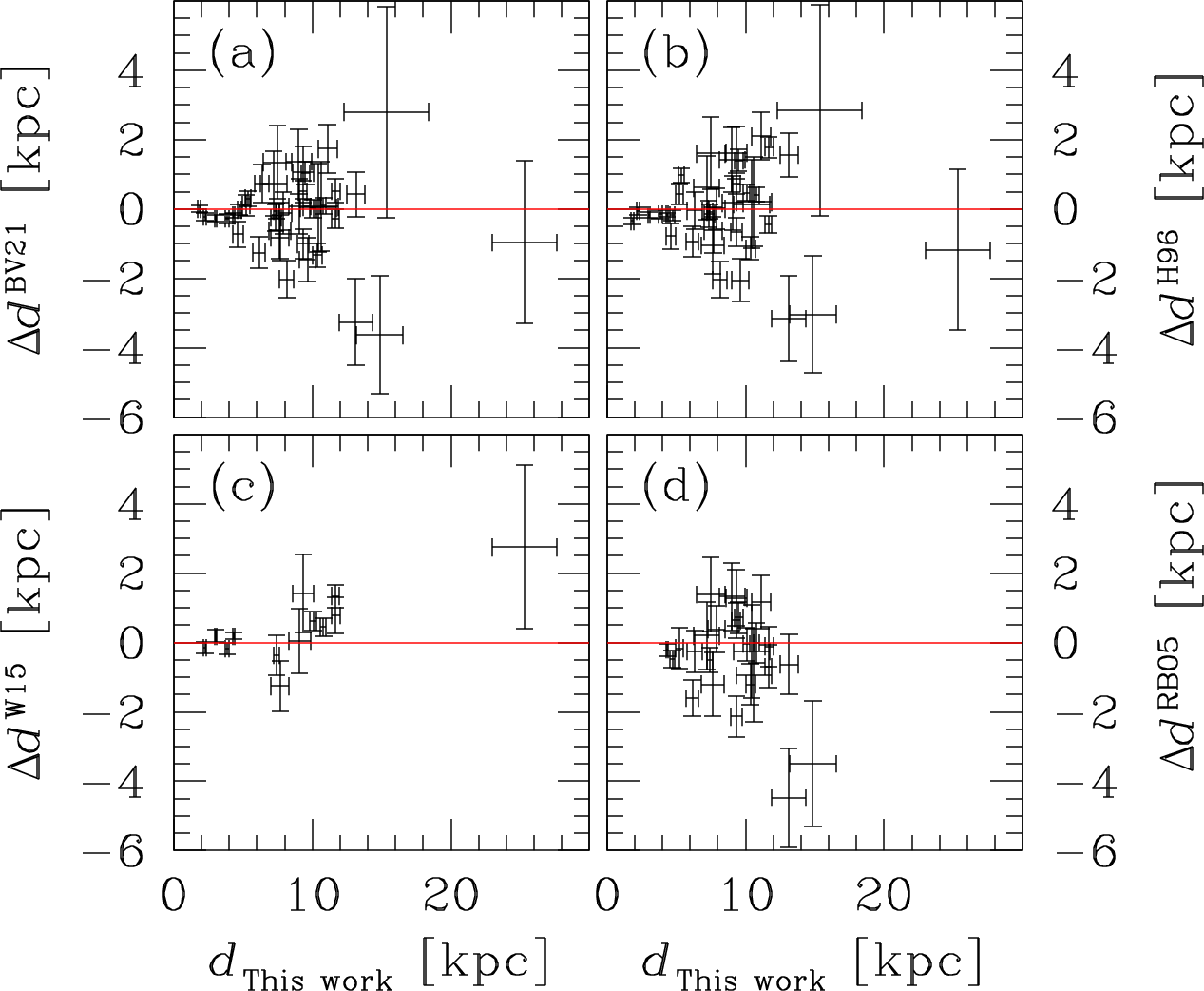
Figure 9: Comparison between our distances and those in the literature: Baumgardt & Vasiliev (2021, panel a), the Harris catalog (panel b), Watkins et al. (2015b, panel c) and Recio-Blanco et al. (2005, panel d). Only error bars are shown for clarity (no error bars are available for distances from the Harris catalog). The red lines are at 0.

6.1 Internal kinematics of mPOPs

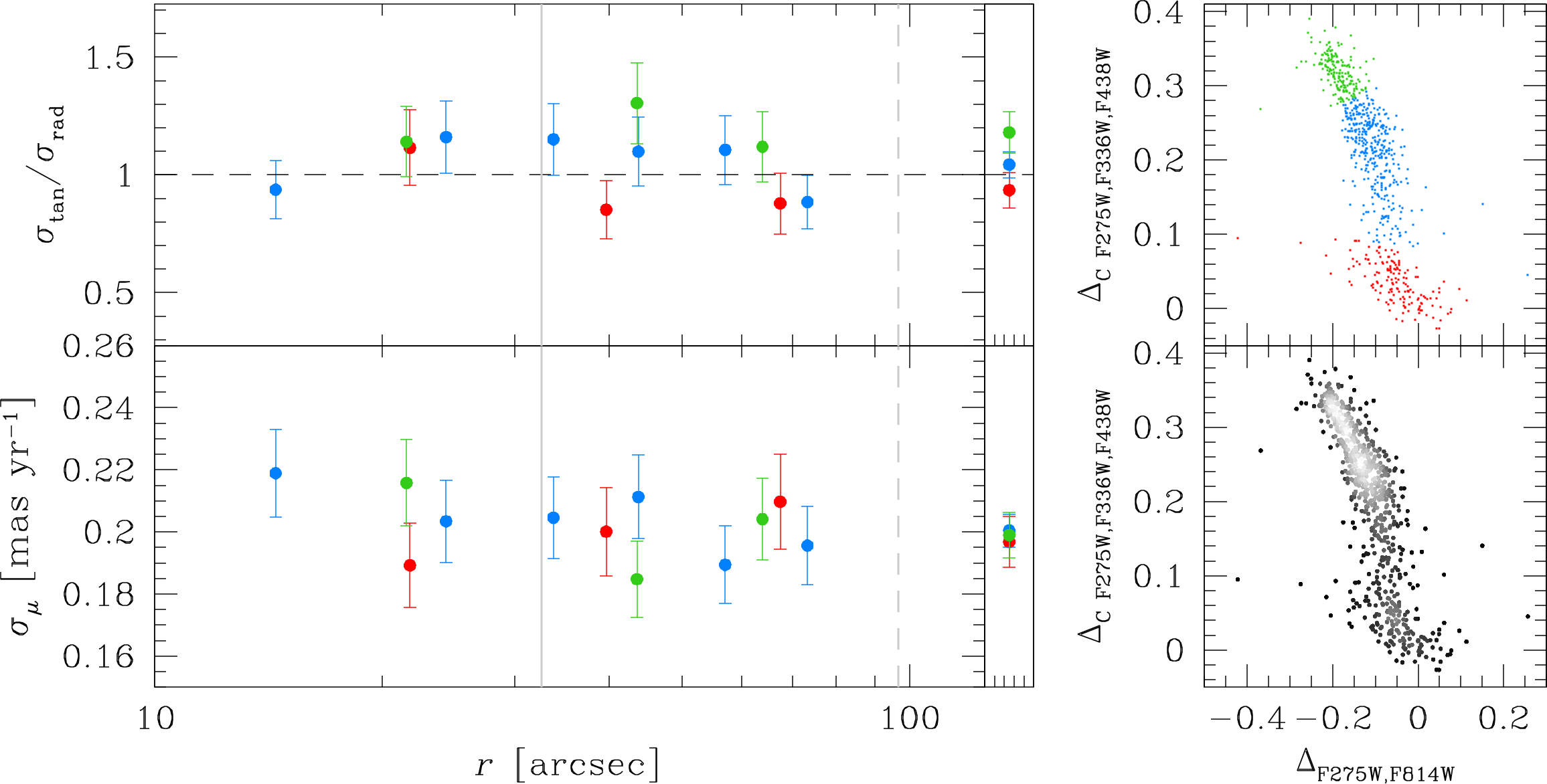
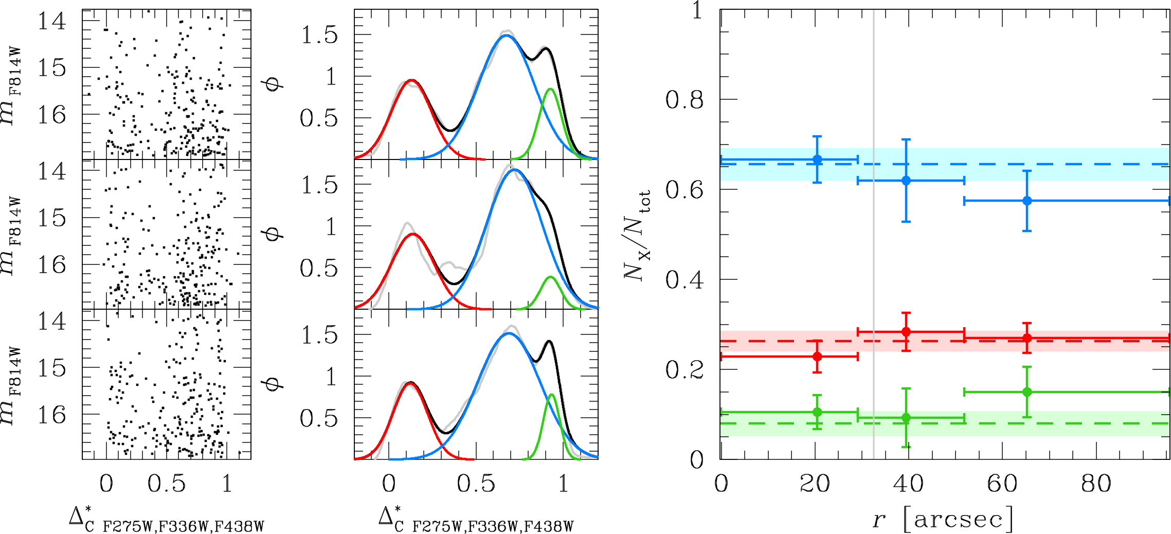
Figure 10: Analysis of the internal kinematics of the mPOPs along the RGB of NGC 5904. We used the chromosome map of Milone et al. (2017) (top-right panel) and an Hess diagram (bottom-right panel) to select three groups of stars: 1G POPa (red points), 2G POPb and POPc (azure and green points, respectively). The left panels show the velocity-dispersion (bottom) and anisotropy (top) radial profiles for each population. 1G and 2G stars are kinematically isotropic and have the same velocity dispersions within our FoV. The gray solid and dashed vertical lines are set the core and half-light radii, respectively. The black, dashed horizontal line in the top-left panel is set to 1 (isotropic case). The small panels next to the left plots present the average velocity dispersion and anisotropy of each population across the entire FoV.

Figure 11: Analysis of the spatial distributions of the mPOPs along the RGB of NGC 5904. The left panels show the $m_{\rm F814W}$ versus $\Delta^{*}_{\rm C\,F275W,F336W,F438W}$ CMDs for stars in each radial bin (with the distance from the center of the cluster increasing from bottom to top). The central panels present the corresponding kernel-density distributions (gray lines) and the triple-Gaussian functions (1G POPa: red; 2G POPb: azure; 2G POPc: green). The sum of the three Gaussians is plotted as a black line. The right panel shows the spatial distributions of the three mPOPs. The horizontal lines (and their shaded regions) correspond to the ratio of each mPOP using all the stars in the field. The vertical, gray line is set at $r_{\rm c}$ ($r_{\rm h}$ is outside the plot boundaries).

Kinematic differences between mPOPs can be a proxy of the different initial formation and evolution of first- (1G) and second-generation (2G) stars (Bekki, 2010; Mastrobuono-Battisti & Perets, 2013, 2016; Hénault-Brunet et al., 2015; Tiongco et al., 2016b, 2019; Vesperini et al., 2013, 2021; Calura et al., 2019; Sollima, 2021). Recently, numerous observational efforts have investigated the kinematic properties of 1G and 2G stars to help us understand the mPOP phenomenon. We now know that 1G and 2G stars share similar kinematic features in dynamically-old GCs, or at least in the centermost regions of GCs where the two-body relaxation time is short, because two-body processes have already erased any kinematic differences between mPOPs (Anderson & van der Marel, 2010; Libralato et al., 2018a, 2019). The outermost regions of GCs are instead less relaxed, and some fingerprints of the initial kinematic differences between mPOPs can still be detected (Richer et al., 2013; Bellini et al., 2015, 2018; Milone et al., 2018; Dalessandro et al., 2018a, b, 2019; Cordoni et al., 2020a, b).

Evidence of the presence of mPOPs in NGC 5904 has been shown both spectroscopically (Ivans et al., 2001; Carretta et al., 2009b; Gratton et al., 2013) and photometrically (Milone et al., 2017; Lee, 2017, 2021). To identify the mPOPs in our field, we made use of the pseudo color-color diagram (“chromosome map”) computed by Milone et al. (2017) for this stellar cluster. We cross-correlated our PM catalog of NGC 5904 with that of Milone et al. (2017) and used their chromosome map to select 1G and 2G stars along the RGB of this cluster (right panels of Fig. 11). We identified three groups of stars: a 1G population (hereafter POPa in red) and two 2G groups (POPb and POPc in azure and green, respectively). The 1G-2G tagging was obtained in a similar way to what is shown in Fig. 4 of Milone et al. (2017). The two 2G sub-populations were arbitrarily identified using the Hess diagram in Fig. 11.

We then measured the velocity dispersions of each population in various radial bins of at least 50 stars each. The velocity-dispersion (bottom-left panel) and anisotropy (top-left panel) radial profiles show that 1G and 2G stars have similar kinematic temperature and are isotropic within our FoV (there is only a marginal hint of a radially and tangentially anisotropic POPa and POPc, respectively). This is expected given that our field covers out to about the half-light radius of the cluster, a region where two-body encounters have likely removed any initial kinematic differences between mPOPs. Our findings are in agreement with those obtained by Cordoni et al. (2020a) with the Gaia DR2 PMs.

This result is in contrast with the finding of Lee (2021), which measured the analog of the POPc stars as more spatially concentrated than the other two populations even within the half-light radius. However, analogously to the internal motions, differences in the spatial segregation of mPOPs can be preserved in regions where the relaxation time is long enough to preserve them. Thus, the complete mixing and similar kinematic features are likely expected for the mPOPs in the core of NGC 5904.

To shed light on this disagreement, we computed the spatial distribution of the three populations in our FoV as follows. First, we divided our sample of RGB stars into three equally-populated bins and computed a kernel-density distribution of the $\Delta^{*}_{\rm C\,F275W,F336W,F438W}$ color for the stars in each bin. The $\Delta_{\rm C\,F275W,F336W,F438W}$ color was obtained Milone et al. (2017) after rectifying the RGB sequences in the $m_{\rm F814W}$ versus ${\rm C_{F275W,F336W,F438W}}$ CMD. However, the sequences have been rectified using all stars in the FoV and, in different radial bins, they can show some deviations from being exactly vertical. Thus, we fine-tuned the $\Delta_{\rm C\,F275W,F336W,F438W}$ color in each radial bin by using two fiducial lines (one each on the red and blue sides of the RGB sequence, respectively) drawn by hand and then computing a new color $\Delta^{*}_{\rm C\,F275W,F336W,F438W}$ as in Libralato et al. (2019, see left panels of Fig. 11):

$$\begin{split}\Delta^{*}_{\rm C\,F275W,F336W,F438W}=\\ =\frac{(\Delta_{\rm C\,F275W,F336W,F438W}-\rm fiducial_{red})}{(\rm fiducial_{blue}-\rm fiducial_{red})}\,.\end{split}$$ (3)

The kernel-density distribution of the $\Delta^{*}_{\rm C\,F275W,F336W,F438W}$ color in each bin was fitted with a triple-Gaussian function (central panels of Fig. 11), and the fraction of stars in each population was estimated following the same approach of Bellini et al. (2013). To ensure the density distribution was robust against the small statistics along the RGB, we obtained the fraction of each mPOP by bootstrapping with replacements the sample of stars 1 000 times. The final values for the fractions of stars and their errors were determined as the median and the 68.27-th percentile of the distribution about the median, respectively. The ratios of the three mPOPs are shown in the right panel of Fig. 11. At odds with the finding of Lee (2021), we can see that the fractions of each mPOP do not vary as a function of distance from the center of the cluster within our FoV, as expected.

6.2 Energy equipartition

The energy-equipartition state of a GC is one of the most challenging measurements to obtain because it requires precise PMs along a (relatively) wide range of masses, i.e., for faint stars. Nowadays, this is one of the few applications that only HST can allow us to investigate in detail.

In collisional systems in a certain state of energy equipartition, there is a relation between the stellar mass $m$ and the velocity dispersion $\sigma_{\mu}$: $\sigma_{\mu}\propto m^{-\eta}$, where $\eta$ is the level of energy equipartition of the system. Theoretical works (Trenti & van der Marel, 2013; Bianchini et al., 2016; Webb & Vesperini, 2017) have shown that a complete state of energy equipartition ($\eta=0.5$) is never reached because of the so-called Spitzer instability. Recent observational works on this topic have verified the goodness of this prediction (Anderson & van der Marel, 2010; Bellini et al., 2018; Libralato et al., 2018a, 2019).

We made use of the exquisite PMs of NGC 5904 to measure its state of energy equipartition using both the parameter $\eta$ defined above and the equipartition mass parameter $m_{\rm eq}$ introduced by Bianchini et al. (2016). As a reference, a high degree of energy equipartition is characterized by a large value of $\eta$ and a small value of $m_{\rm eq}$.

We started by inferring the mass of stars along the MS below the MS turnoff by means of the updated isochrones of the “A Bag of Stellar Tracks and Isochrones” (BaSTI; Hidalgo et al., 2018). The parameters for NGC 5904 were chosen from the recent work of Gontcharov et al. (2019): a solar-scaled, 12.15 Gyr old isochrone for $[$Fe$/$H$]=-1.33$, $Y=0.2478$, accounting for atomic diffusion, with a distance of 7.4 kpc. The fit is shown in Fig. 13. Although not perfect for the faintest portion of the MS due to the still-existing shortcomings in this mass regime of the color-effective temperature relationship, the fit is good enough to assign a mass to each star.

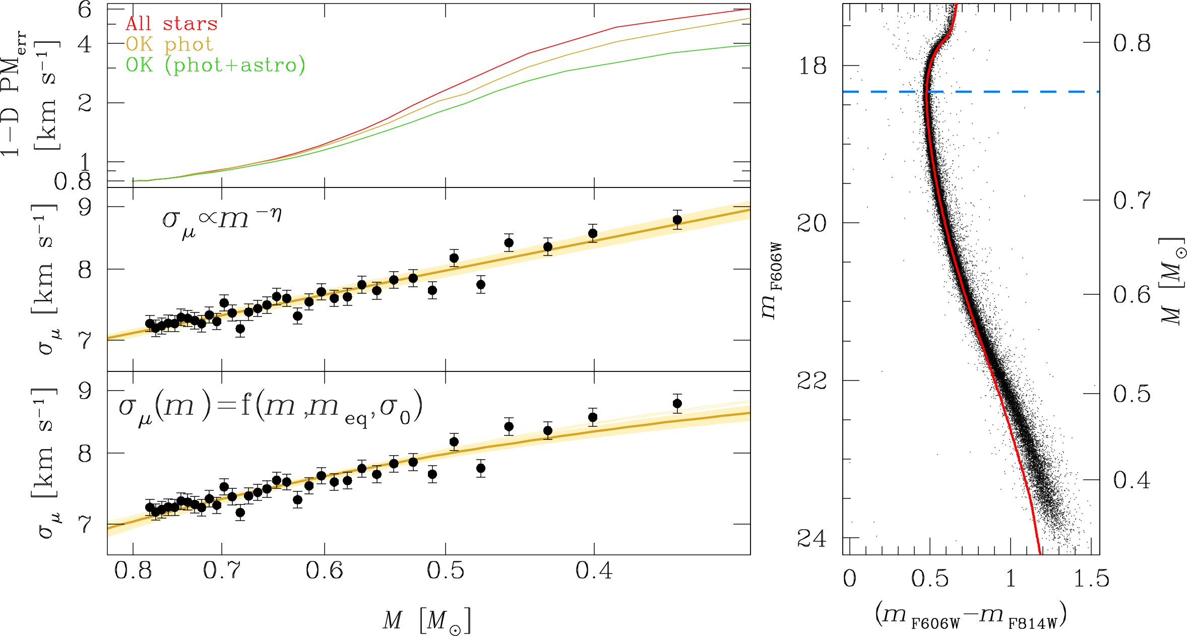
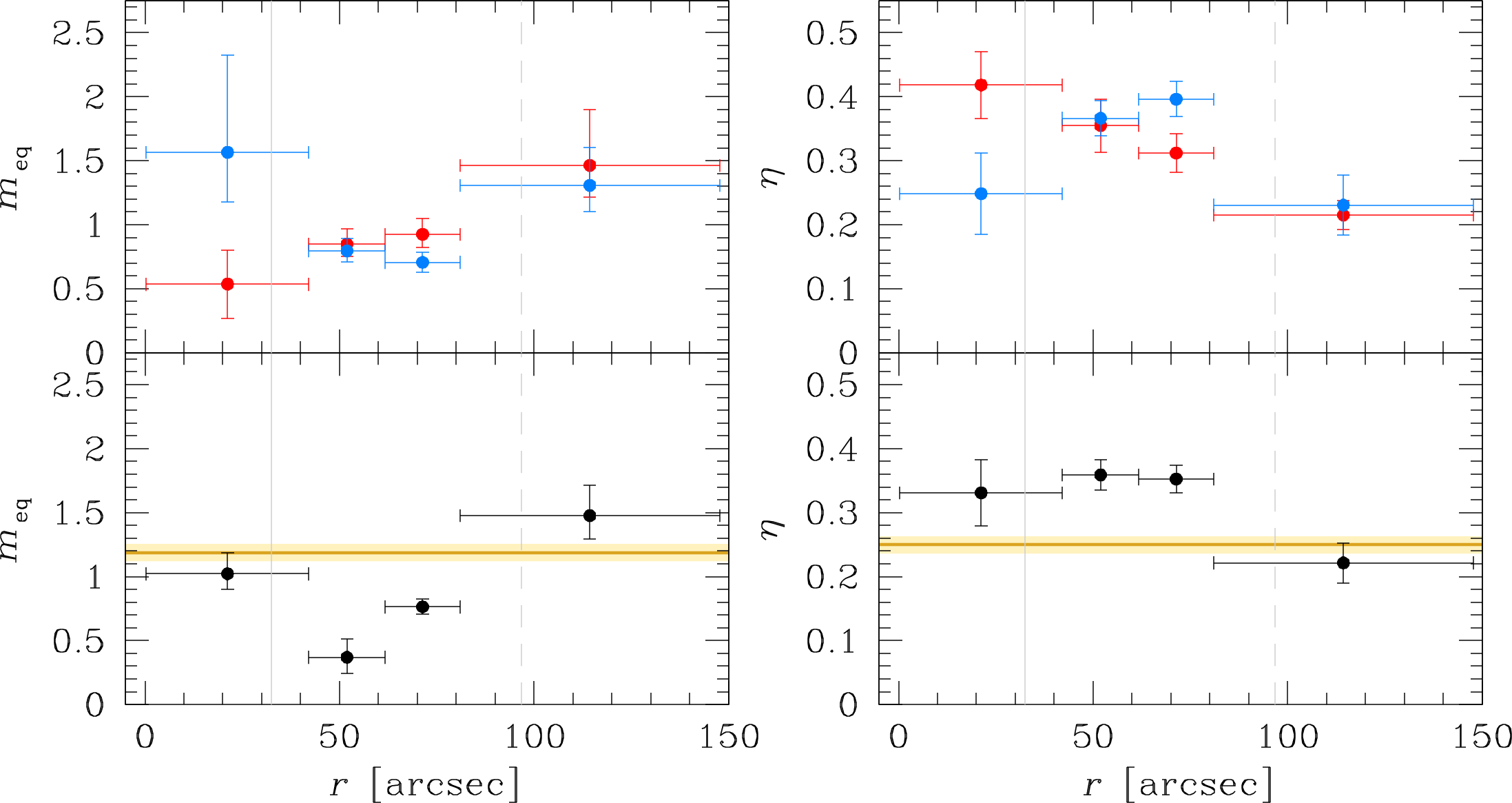
Figure 12: Measurement of the level of energy equipartition in NGC 5904. In the CMD on the right, we show in red the isochrone used to estimate the mass of the stars along the MS. In the left panels, we show the velocity dispersion $\sigma_{\mu}$ as a function of mass for MS stars. The gold line is the best fit obtained with the scale parameter $m_{\rm eq}$ (bottom panel) or the classical formalism of $\eta$ (middle panel). The yellow regions correspond to the 1$\sigma$ errors of the fit. The top-left panel presents the median 1-D PM error as a function of stellar mass for three samples: all objects in the catalog (red line), sources that passed our photometric quality selections (yellow line), and stars that survived both the photometric and astrometric cuts (green line).

Figure 13: Local levels of energy equipartition of NGC 5904. Left panels show the value of $m_{\rm eq}$ as a function of distance from the center of the cluster, while right panels present the same trend for $\eta$. Bottom panels are obtained by considering the combined velocity dispersion $\sigma_{\mu}$. The gold line and the yellow region represent the global value of the level of energy equipartition and its 1$\sigma$ region as measured in Fig. 13. In the top panels, we highlight the trends obtained by estimating the level of energy equipartition using either the radial component $\sigma_{\rm rad}$ (red points) or the tangential component $\sigma_{\rm tan}$ (blue points).

We then computed the $\sigma_{\mu}$ in 35 bins of 1077 stars each along the MS. The bottom-left panel of Fig. 13 shows the result obtained by fitting the mass-dependent exponential relation of Bianchini et al. (2016) with a maximum-likelihood approach. We find a global $m_{\rm eq}=1.18\pm 0.07$ $M_{\odot}$. Bianchini et al. (2016) provided a relation between $m_{\rm eq}$ and the ratio between the cluster age and its core relaxation time. Using the age of Gontcharov et al. (2019) and a core relaxation time of 0.19 Gyr (Harris, 1996, 2010 edition), we expect a value of $m_{\rm eq}=1.67^{+0.32}_{-0.28}$ $M_{\odot}$, which is in agreement with our estimate at the 2$\sigma$ level.

The middle-left panel presents the linear fit in the same log-log plane. We found a value of $\eta=0.25\pm 0.01$. As for the value of $m_{\rm eq}$, this finding is consistent with the theoretical predictions of a partial state of energy equipartition even in an advanced stage of the cluster evolution.

As a reference, the median 1-D PM error as a function of stellar mass is plotted in the top-left panel of Fig. 13. The three lines correspond to the median PM trends of: all objects in the catalog (red line), sources that passed our photometric quality selections (see Sect. 4; yellow line), and stars that survived both the photometric and astrometric cuts (always described in Sect. 4; green line).

Our data set allowed us to push this investigation even further. We divided our FoV in four equally-populated radial bins, and measured the level of energy equipartition in each bin using the velocity dispersions measured in ten equally-populated magnitude bins. The result is shown in the bottom panels of Fig. 13 (left for $m_{\rm eq}$ and right for $\eta$). We can notice marginal evidence of the innermost regions of the cluster having a higher degree of energy equipartition (low $m_{\rm eq}$ and high $\eta$) than the outskirts. The innermost point within $r_{\rm c}$ is the most uncertain because the fit is obtained with a smaller mass baseline.

In the top panels, we reproduce a similar analysis, but this time measuring the level of energy equipartition using the radial and tangential components of the velocity dispersion separately. We find that the levels of energy equipartition from $\sigma_{\rm rad}$ and $\sigma_{\rm tan}$ are consistent with each other at all radii, with only marginal differences at the 1–2$\sigma$ level. The larger difference between the level of energy equipartition in the two components is shown in the innermost bin. The discrepancy is mainly the result of a poor fit, especially in the case of the exponential fit. This is in agreement with the simulations of Pavlík & Vesperini (2021, 2022) who found the degree of energy equipartition in the two velocity components to be similar in the region within the half-light radius. Future studies will extend the investigation of the energy equipartition in the tangential and radial dispersions to the outer regions of GCs where, according to Pavlík & Vesperini (2021, 2022), the degrees of energy equipartition in these two velocity components may differ.

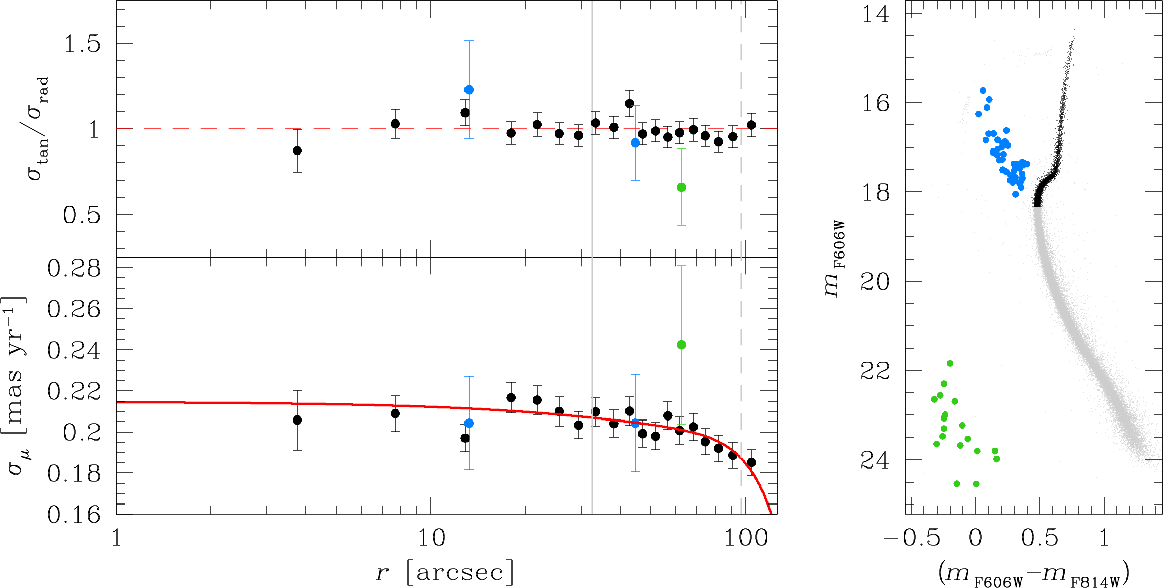
Figure 14: The optical CMD of NGC 5904 is shown in the right panel. Black dots are the reference population used in the analysis (Sect. 6.3), blue dots are BSs, and green points correspond to WDs. All other objects are shown as gray dots. In the bottom-left panel, we show the velocity-dispersion radial profiles of the the reference population (in black), BSs (in blue) and WDs (in green). The red line is the polynomial fit to the $\sigma_{\mu}$ of the reference population. The top-left panel presents the anisotropy radial profile for the same stars. The red, dashed horizontal line is set to 1. In all the left panels of this Figure, the vertical lines mark the $r_{\rm c}$ (solid) and $r_{\rm h}$ (dashed).

A note on the PM errors for faint stars

Despite our careful data reduction and PM computation, the PM errors might be under/overestimated. For example, a higher velocity dispersion for faint stars could be caused by underestimated PM uncertainties. We repeated the analysis shown in Fig. 13 by using only stars brighter than (1) $m_{\rm F606W}=22.1$ ($\sim 0.5M_{\odot}$) and (2) $m_{\rm F606W}=23.2$ ($\sim 0.42M_{\odot}$). We find:

• $m_{\rm F606W}\leq 22.1$ ($M\gtrsim 0.5M_{\odot}$): $m_{\rm eq}=1.60\pm 0.18$ $M_{\odot}$ , $\eta=0.21\pm 0.02$ ;

• $m_{\rm F606W}\leq 23.2$ ($M\gtrsim 0.42M_{\odot}$): $m_{\rm eq}=1.31\pm 0.10$ $M_{\odot}$ , $\eta=0.24\pm 0.02$ .

Although the results are in agreement at the 1–2$\sigma$ level, it seems that the value of $m_{\rm eq}$ is larger ($\eta$ is smaller) the brighter is the magnitude cut, i.e., when we exclude the faintest objects with large PM errors. However, the exponential fit is less robust when the mass interval is small (the associated errors increase). The variation of $\eta$ is instead mild.

Furthermore, the selections applied can bias the analyzed sample and the inferred kinematics, as extensively discussed in Bellini et al. (2014). In the case of NGC 5904, we find that the selection on the PM reduced $\chi^{2}$ applies a more significant cut on the PM errors, as shown in the top panel of Fig. 13 by the comparison of the yellow and green lines. As a test, we repeated the same analysis as before upon rescaling the PM errors of the stars used in the measurement of the level of energy equipartition by the ratio between the median PM errors obtained with sources that passed our photometric quality selections (yellow line in the top panel of Fig. 13), and with stars that survived both the photometric and astrometric cuts (green line). We find a global level of energy equipartition of $m_{\rm eq}=1.50\pm 0.11$ $M_{\odot}$ and $\eta=0.20\pm 0.01$. Since we increased the PM errors, the intrinsic velocity dispersion of faint stars decreased, but again all estimates are in agreement within 2–3$\sigma$.

It is hard to say if these tests are a proxy of underestimated PM errors for faint stars,if they are biased by the less-constrained fit, or if what we see is just due to the intrinsic kinematics of our tracers. Nevertheless, these examples highlight how important it is to understand the data set used. Once again, we advise users to carefully check the PMs, and test their quality selections on a cluster-by-cluster basis, especially when the PM errors are of the order of the intrinsic velocity dispersion of the stars.

6.3 Kinematic mass determination

Knowledge of the relation between mass and velocity dispersion allows us to measure the kinematic mass of stars, similar to what has been done by Baldwin et al. (2016) and Libralato et al. (2018a, 2019). The unknown mass of a group of stars X ($M_{\rm X}$) with velocity dispersion $\sigma_{\rm X}$ can be obtained as follows:

$$\alpha_{\rm X}=\frac{\sigma_{\rm X}}{\sigma_{\rm ref}}=\left(\frac{M_{\rm X}}{M_{\rm ref}}\right)^{-\eta}\,,$$ (4)

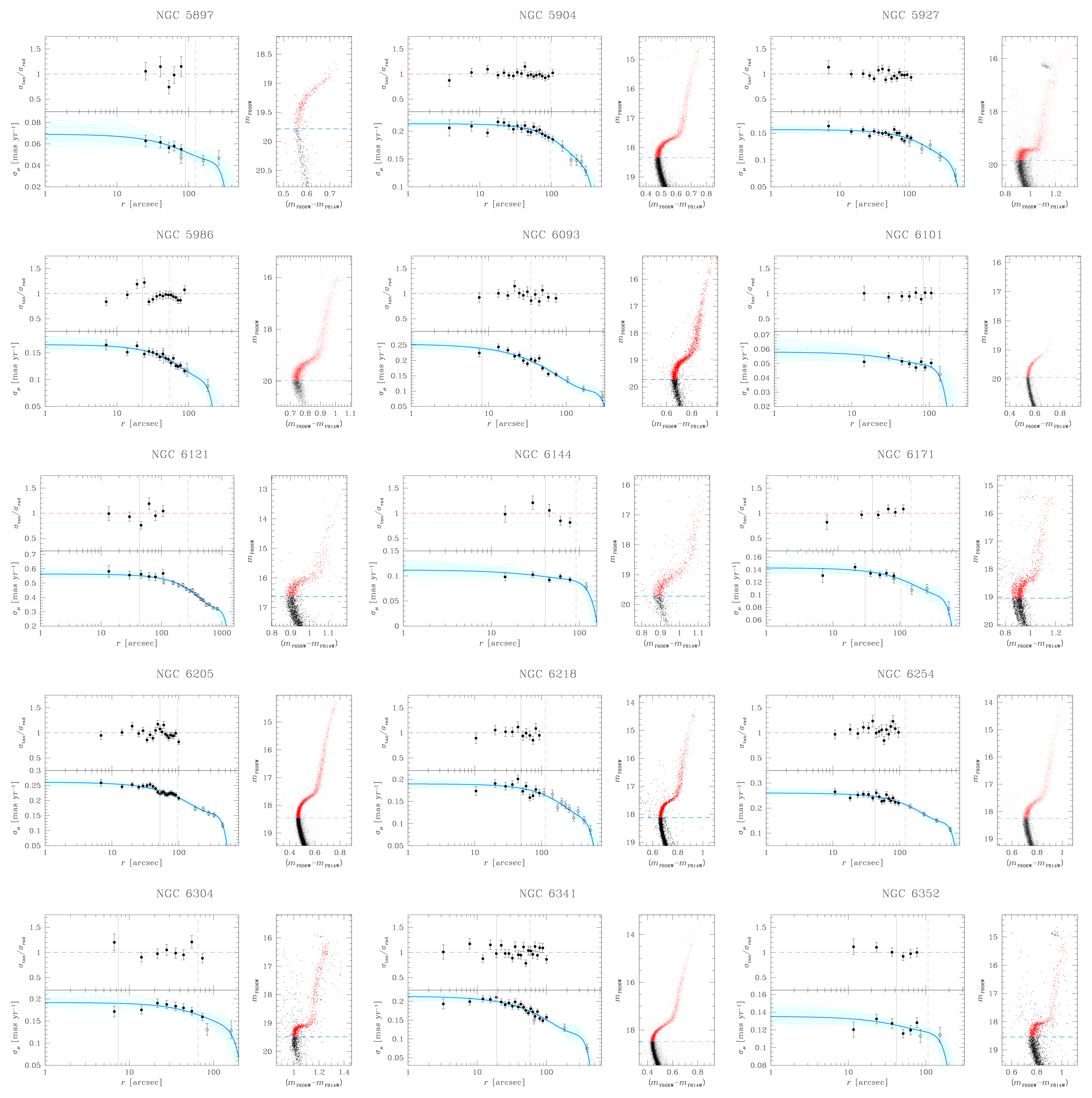
Figure A3: Similar to Fig. A2, but for NGC 5897, NGC 5904, NGC 5927, NGC 5986, NGC 6093, NGC 6101, NGC 6121, NGC 6144, NGC 6171, NGC 6205, NGC 6218, NGC 6254, NGC 6304, NGC 6341, and NGC 6352. The CMD of NGC 5897 is cut at the SGB level because only one exposure mapping the RGB is available in the GO-10775 data. Having only two epochs at our disposal for this GC, the PM fit for these bright stars would have been forced to pass through the only first-epoch point, thus making the PM measurement uncertain.

where $M_{\rm ref}$ and $\sigma_{\rm ref}$ are the known mass and velocity dispersion of a reference population. For this analysis, we choose to measure the mass of two groups of stars: blue stragglers (BSs) and white dwarfs (WDs). Our reference population is the stars brighter than MS turnoff along the SGB and RGB (the same stars analyzed in Fig. A3), for which we assume $M_{\rm ref}$ to be equal to the mass of stars at the MS turnoff. Using the isochrone in Sect. 6.2, we define $M_{\rm ref}=0.78$ $M_{\odot}$.

We selected BSs and WDs in various optical and UV CMDs (right panel of Fig. 14). We split the BSs into two groups (of 22 and 21 stars, respectively) and WDs into one group (of 14 stars), and measured their velocity dispersions $\sigma_{\mu}$. The result is shown in the bottom-left panel of Fig. 14. Blue points depict the velocity dispersions of the BSs, while the green dot refers to the WD kinematics. Black points are the reference population. The effect of the energy equipartition is shown in the plot: BSs, which are more massive than RGB, SGB and MS stars, seem to be slightly kinematically colder (lower $\sigma_{\mu}$) than the reference population. WDs have a mass of about 0.5 $M_{\odot}$ (e.g., Bedin et al., 2019, and references therein). Being less massive than the reference population, their $\sigma_{\mu}$ is instead marginally higher. Finally, the top-left panel shows that BSs and WDs are kinematically isotropic as the other stars at the $\sim$1$\sigma$ level.

We previously fit the $\sigma_{\mu}$ of the reference population with a polynomial function (see Sect. 4). To obtain the mass of the BSs, we repeated the same computation but we also solved for $\alpha_{\rm BS}$ by rescaling the polynomial of the reference population to fit the BS $\sigma_{\mu}$ at the same time. By assuming the global value of $\eta=0.25\pm 0.01$, we obtain $M_{\rm BS}=0.84\pm 0.28$ $M_{\odot}$. However, we notice that the BSs are preferentially located in regions where the local level of energy equipartition is higher than the global level. If we use the average value of $\eta$ in these regions ($0.34\pm 0.06$), the mass becomes $M_{\rm BS}=0.82\pm 0.20$ $M_{\odot}$. The difference between the two values is small since the value of $\alpha_{\rm BS}$ is close to unity. Both estimates are in agreement with the BS mass of NGC 5904 obtained by Baldwin et al. (2016, $0.82^{+0.29}_{-0.18}$ $M_{\odot}$). The mass of the BSs in this cluster is slightly lower than the average BS mass (1.0–1.6 $M_{\odot}$; e.g., Ferraro et al., 2018). However, it is worth noticing that our sample is mainly composed of BSs close to the MS turnoff, which are less massive than those on the bright-end of the BS sequence (e.g., Raso et al., 2019).

For the WDs, a robust analysis cannot be obtained because we have only one point at our disposal for deriving $\alpha_{\rm WD}$. Nevertheless, we repeated the same analysis to qualitatively assess the mass of the WDs. If we use the global value of $\eta$, we obtain $M_{\rm WD}=0.39\pm 0.25$ $M_{\odot}$, which is lower than the average mass of the WDs in GCs. However, if we assume the local level of energy equipartition at the average WD distance from the center of the cluster, we find $M_{\rm WD}=0.48\pm 0.21$ $M_{\odot}$.

7 Conclusions

We computed PMs for 57 stellar clusters studied in the GO-13297 program. The astro-photometric catalogs taht we have made publicly available represent the most complete, homogeneous collection of PMs of stars in the cores of stellar clusters to date, and more than double the number of clusters for which high-precision, HST-based PMs are available (Bellini et al., 2014). Furthermore, the astrometric information that we are releasing is complementary to that provided by the current (and future) Gaia data releases. At the dawn of a new era in astronomy with the first light of the James Webb Space Telescope (JWST), the legacy that these PM catalogs offer is further enhanced, since they can serve as an important astrometric benchmark for JWST-based data reduction and tools.

We described the data reduction and, in great detail, the quality selections needed to select reliable objects for any kinematic analysis. We stress again that the data used for each cluster are different, thus any correction or selection should be tailored on a cluster-by-cluster basis. This is particularly important for stars with PM errors of the same order as the amplitude of the kinematic features that one wants to measure, for example, for stars along the MS of GCs.

We made use of our catalogs to study the general kinematic properties of the bright, massive stars in our clusters. We provided additional evidence supporting early findings that dynamically-young systems have a radially anisotropic velocity distribution at the half-light radius, while in dynamically older clusters the velocity distribution is isotropic at the same distance from the center of the cluster. This trend is consistent with the theoretical results of simulations showing that initially radially anisotropic clusters evolve toward an isotropic velocity distribution during their long-term evolution. Interestingly, core-collapsed clusters show similar properties to the non-core-collapsed systems, although a larger sample of core-collapsed GCs will be necessary to confirm the similarities with non-core-collapsed clusters (in particular for the group with longer relaxation times).

Finally, we showcased our PM catalogs using the GC NGC 5904. We separated the mPOPs along the RGB of the cluster and showed that, within our FoV, 1G and 2G stars have the same kinematics, are kinematically isotropic and have the same flat radial distributions. A detailed analysis of the kinematics of mPOPs will be the subject of another paper in this series.

We investigated in detail the level of energy equipartition of NGC 5904. This cluster is in an advanced stage of its dynamical evolution, yet it has reached only a partial state of energy equipartition, as predicted by theoretical simulations. Knowledge of the level of energy equipartition also allowed us to measure the kinematic masses the BSs and WDs, finding a good agreement with the typical masses of these objects obtained with different methods in the literature.

Appendix A Absolute PMs

We cross-correlated each of our PM catalogs with the Gaia EDR3 catalog and computed the PM zero-points to transform our relative PMs onto an absolute system.

We considered only cluster members with well-measured HST PMs (see Sect. 4) and whose Gaia EDR3 PMs have an RUWE better than 1.25, an astrometric excess noise less than 0.4, a number of bad along-scan observations less than 1.5% of the total number of along-scan observations, a PM error in each coordinate better than 0.1 mas yr^-1, and $G>13$. If fewer than 25 objects were found in common with our HST sample, we relaxed these parameters to increase the statistics. The PM zero-point in each coordinate is defined as the 3.5$\sigma$-clipped average value of the difference between the HST and Gaia PMs. We set the error equal to the error of the mean. We also added in quadrature to our uncertainties a systematic error for the Gaia EDR3 PMs of 0.026 mas yr^-1 (obtained using Eq. 2 of Vasiliev & Baumgardt, 2021, assuming an angular separation $\theta=0$ deg since we are analyzing the clusters’ cores). We do not take into account the rotation of the clusters in the plane of the sky, which is included in the PMs from the Gaia catalog but not in those made with the HST data (Sect. 3), although the scatter due to this effect is small. All values are reported in Table A1.

This astrometric registration allows us to directly compare our PMs with those in the Gaia EDR3 catalog. We show the result in Fig. A1. The red lines are the plane bisectors, not a fit to the data. The tight alignment of the points to the plane bisectors shows that our PMs are consistent with those of the Gaia EDR3 catalog, and that our absolute registration is accurate. The large scatters along the $y$ directions are due to the poor quality of the Gaia PMs in some clusters, likely because of crowding.

Table A1: PM zero-point needed to transform our relative HST PMs onto an absolute reference frame. These values correspond to the absolute PM of each cluster. Uncertainties include both the statistical errors and Gaia EDR3 systematic errors.

Cluster	$\Delta(\mu_{\alpha}\cos\delta,\mu_{\delta})$	Cluster	$\Delta(\mu_{\alpha}\cos\delta,\mu_{\delta})$
	$[$mas yr-1$]$		$[$mas yr-1$]$
NGC 104	$(5.385\pm 0.056,-2.340\pm 0.047)$	NGC 6352	$(-2.168\pm 0.028,-4.416\pm 0.028)$
NGC 288	$(4.154\pm 0.029,-5.711\pm 0.028)$	NGC 6362	$(-5.504\pm 0.027,-4.752\pm 0.028)$
NGC 362	$(6.737\pm 0.039,-2.522\pm 0.032)$	NGC 6366	$(-0.346\pm 0.030,-5.176\pm 0.029)$
NGC 1261	$(1.577\pm 0.032,-2.068\pm 0.035)$	NGC 6388	$(-1.304\pm 0.029,-2.706\pm 0.031)$
NGC 1851	$(2.128\pm 0.031,-0.646\pm 0.032)$	NGC 6397	$(3.231\pm 0.027,-17.641\pm 0.027)$
NGC 2298	$(3.270\pm 0.032,-2.165\pm 0.032)$	NGC 6441	$(-2.571\pm 0.043,-5.312\pm 0.040)$
NGC 2808	$(0.927\pm 0.054,0.336\pm 0.098)$	NGC 6496	$(-3.088\pm 0.037,-9.265\pm 0.035)$
NGC 3201	$(8.348\pm 0.029,-1.965\pm 0.029)$	NGC 6535	$(-4.220\pm 0.030,-2.923\pm 0.033)$
NGC 4590	$(-2.713\pm 0.029,1.746\pm 0.030)$	NGC 6541	$(0.301\pm 0.030,-8.851\pm 0.032)$
NGC 4833	$(-8.395\pm 0.031,-0.952\pm 0.031)$	NGC 6584	$(-0.111\pm 0.031,-7.202\pm 0.028)$
NGC 5024	$(-0.177\pm 0.033,-1.349\pm 0.039)$	NGC 6624	$(0.145\pm 0.031,-6.944\pm 0.032)$
NGC 5053	$(-0.333\pm 0.033,-1.198\pm 0.034)$	NGC 6637	$(-5.026\pm 0.031,-5.818\pm 0.031)$
NGC 5272	$(-0.261\pm 0.055,-2.674\pm 0.040)$	NGC 6652	$(-5.491\pm 0.032,-4.237\pm 0.029)$
NGC 5286	$(0.271\pm 0.044,-0.156\pm 0.049)$	NGC 6656	$(9.758\pm 0.063,-5.665\pm 0.036)$
NGC 5466	$(-5.371\pm 0.030,-0.800\pm 0.031)$	NGC 6681	$(1.409\pm 0.030,-4.707\pm 0.030)$
NGC 5897	$(-5.470\pm 0.059,-3.405\pm 0.051)$	NGC 6715	$(-2.691\pm 0.032,-1.363\pm 0.030)$
NGC 5904	$(4.079\pm 0.036,-9.876\pm 0.036)$	NGC 6717	$(-3.086\pm 0.039,-5.003\pm 0.040)$
NGC 5927	$(-5.058\pm 0.028,-3.188\pm 0.028)$	NGC 6723	$(1.021\pm 0.033,-2.430\pm 0.032)$
NGC 5986	$(-4.258\pm 0.036,-4.569\pm 0.033)$	NGC 6752	$(-3.155\pm 0.027,-4.010\pm 0.028)$
NGC 6093	$(-2.885\pm 0.052,-5.665\pm 0.040)$	NGC 6779	$(-1.988\pm 0.031,1.595\pm 0.031)$
NGC 6101	$(1.756\pm 0.028,-0.245\pm 0.030)$	NGC 6791	$(-0.421\pm 0.026,-2.273\pm 0.026)$
NGC 6121	$(-12.509\pm 0.028,-19.012\pm 0.028)$	NGC 6809	$(-3.434\pm 0.029,-9.315\pm 0.028)$
NGC 6144	$(-1.755\pm 0.031,-2.607\pm 0.031)$	NGC 6838	$(-3.416\pm 0.027,-2.655\pm 0.028)$
NGC 6171	$(-1.932\pm 0.029,-5.976\pm 0.028)$	NGC 6934	$(-2.629\pm 0.035,-4.687\pm 0.035)$
NGC 6205	$(-3.130\pm 0.035,-2.505\pm 0.047)$	NGC 6981	$(-1.231\pm 0.036,-3.332\pm 0.031)$
NGC 6218	$(-0.185\pm 0.028,-6.796\pm 0.028)$	NGC 7078	$(-0.645\pm 0.032,-3.803\pm 0.032)$
NGC 6254	$(-4.766\pm 0.030,-6.609\pm 0.028)$	NGC 7089	$(3.458\pm 0.139,-2.269\pm 0.076)$
NGC 6304	$(-4.126\pm 0.039,-1.004\pm 0.035)$	NGC 7099	$(-0.718\pm 0.031,-7.305\pm 0.030)$
NGC 6341	$(-4.934\pm 0.031,-0.635\pm 0.032)$

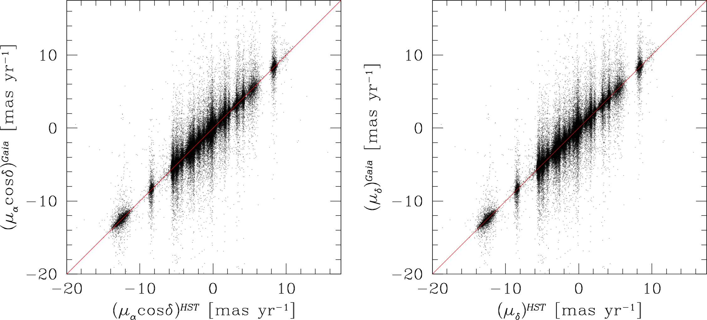
Figure A1: Comparison between the HST (including the PM zero-points in Table A1) and Gaia PMs. The red lines are the plane bisectors, not a fit to the data.

Appendix B Description of the publicly available catalogs

We release the astro-photometric catalogs of the 57 stellar clusters of the GO-13297 program through the MAST archive. Table A2 presents the columns of our PM catalogs. For each cluster, we also release the photometric catalogs obtained with the second-pass photometry discussed in Sect. 2 for each filter/camera/epoch the data of which were used to compute the PMs. These catalogs will allow users to reproduce the quality selections we applied in Sect. 4. The description of a typical photometric catalog is provided in Table A3.

When using our catalogs, users might notice peculiar features in some CMDs. For example, there are some filter combinations that show a clear, yet nonphysical, split in the SGB and RGB. The sources in these anomalous branches are close to the saturation and present large QFIT and RADXS values, so they can be easily removed from the analysis.

Our photometric catalogs can contain saturated stars for a given epoch/camera/filter if these sources are not saturated in at least two other epoch/camera/filter combinations so as to enable a PM measurement. As discussed in Bellini et al. (2017a), KS2 does not deal with saturated pixels, and photometry for saturated stars is instead provided by the first-pass stage of data reduction. Even though the photometric systems of saturated and unsaturated stars were designed to be the same, we have sometimes noticed differences between the regions in the CMDs dominated by objects belonging to either of the groups. These differences can be small zero-points (thus creating a discrete discontinuity in the CMD) or more complex behaviors (like a spread in the CMD or a different RGB slope with respect to that of the unsaturated objects). Caution is again advised when dealing with saturated sources.

The photometry of the same camera/filter at different epochs is registered on to the same VEGA-mag system. Small zero-point variations can still be present, but they are expected to be small ($\sim$0.01-0.02 mag, i.e., of the order of the uncertainty in the VEGA-mag calibration).

The astro-photometric catalogs of NGC 362 were made public by Libralato et al. (2018a). We include these same catalogs in our online repository, and refer readers to the related paper for their description. For NGC 6352, we provide the astro-photometric catalogs used in Libralato et al. (2019).

Table A2: Description of a PM catalog.

Column	Name	Unit	Description
1	R.A.	deg	Right Ascension
2	Dec.	deg	Declination
3	X	pixel	X master-frame position (in pixel; pixel scale of 40 mas pixel-1)
4	Y	pixel	Y master-frame position (in pixel; pixel scale of 40 mas pixel-1)
5	$\mu_{\alpha}\cos\delta$	mas yr-1	Corrected PM along $\alpha\cos\delta$
6	$\sigma_{\mu_{\alpha}\cos\delta}$	mas yr-1	Error on the corrected PM along $\alpha\cos\delta$
7	$\mu_{\delta}$	mas yr-1	Corrected PM along $\delta$
8	$\sigma_{\mu_{\delta}}$	mas yr-1	Error on the corrected PM along $\alpha\cos\delta$
9	$\chi^{2}_{\mu_{\alpha}\cos\delta}$		Reduced $\chi^{2}$ of the PM fit along $\alpha\cos\delta$
10	$\chi^{2}_{\mu_{\delta}}$		Reduced $\chi^{2}$ of the PM fit along $\delta$
11	$N_{\rm f}^{\rm PM}$		Number of exposures initially considered in the PM fit
12	$N_{\rm u}^{\rm PM}$		Number of exposures actually used in the PM fit
13	$\Delta{\rm time}$	yr	Temporal baseline of the PM fit
14	$(\mu_{\alpha}\cos\delta)_{\rm raw}$	mas yr-1	Raw PM along $\alpha\cos\delta$
15	$(\sigma_{\mu_{\alpha}\cos\delta})_{\rm raw}$	mas yr-1	Error on the raw PM along $\alpha\cos\delta$
16	$(\mu_{\delta})_{\rm raw}$	mas yr-1	Raw PM along $\delta$
17	$(\sigma_{\mu_{\delta}})_{\rm raw}$	mas yr-1	Error on the raw PM along $\delta$
18	Corr_Flag		Flags that tells if the PM is a-posteriori corrected for systematics
19	ID		ID number of the source

• Note. (i) The ID number of a source is the same in all catalogs for the same cluster. (ii) (X,Y) positions are defined at a specific epoch about halfway between the first and last epochs used in the PM computation. This reference epoch is provided in the header of the file. (iii) “Corr_Flag” is set to 1 if the PM was a-posteriori corrected for high-frequency systematics, and to 0 if otherwise.

Table A3: Description of a photometric catalog for one filter/camera/epoch.

Column	Name	Description
1	$m$	Calibrated VEGA magnitude
2	$\sigma_{m}$	Photometric rms
3	QFIT	Quality-of-PSF-fit (QFIT) parameter
4	$o$	Fractional flux within the fitting radius prior to neighbor subtraction
5	$N_{\rm f}^{\rm phot}$	Number of exposures in which a source was found
6	$N_{\rm u}^{\rm phot}$	Number of exposures used to measure the flux of a source
7	RADXS	Excess/deficiency of flux outside the core of the star
8	sky	Sky in electrons
9	$\sigma_{\rm sky}$	Sky rms in electrons
10	sat	Saturation flag
11	ID	ID number of the source

• Note. (i): The ID number of a source is the same in all catalogs for the same cluster. (ii): All the values for a source are set to 0 if it is not measured in this filter/camera/epoch (iii) All the values for a source except the calibrated magnitude are set to 0 if it is saturated in this catalog. (iv): The saturation flag is set to 9 if the star is saturated. If multiple exposure times are present in the data set, the saturation flag is 0 for a measurement obtained from the longest exposure(s), and progressively increases (by 1) with the decreasing exposure time of the image(s) from which it was measured. (v) To estimate the significance of a source over the sky, first convert the calibrated VEGA magnitudes into instrumental fluxes (in units of electrons): flux $=$ $10^{-0.4({\rm mag}-{\rm VEGA\_zp})}$ The VEGA-magnitude zero-point is provided in the header of the catalog.

Appendix C Kinematic profiles and table

In this Section, we present velocity-dispersion and anisotropy radial profiles. We refer to Sect. 4 for the detailed description of Figs. A2, A3, A4, and A5. Table A4 provides the values of $\sigma_{\mu}$ at $r=0$ arcsec, $r_{\rm c}$ and $r_{\rm h}$. The individual measurements are available on our website.

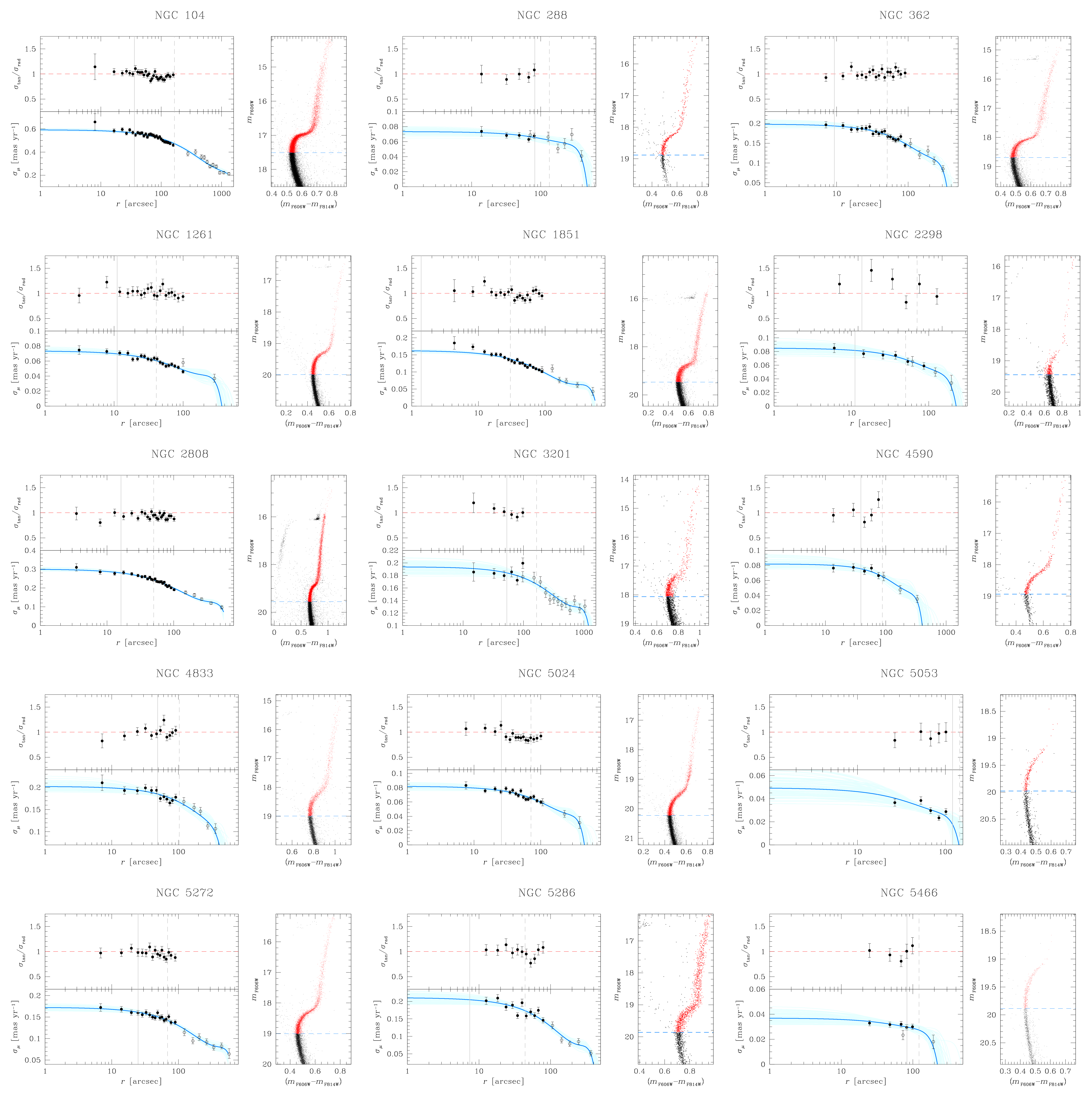
Figure A2: Velocity-dispersion and anisotropy radial profiles for NGC 104, NGC 288, NGC 362, NGC 1251, NGC 1851, NGC 2298, NGC 2808, NGC 3201, NGC 4590, NGC 4833, NGC 5024, NGC 5053, NGC 5272, NGC 5286 and NGC 5466. For each cluster, an $m_{\rm F606W}$ versus $(m_{\rm F606W}-m_{\rm F814W})$ CMD is shown. Red points are stars used for the kinematic analysis, while black dots represent all other objects. The azure, dashed, horizontal line is set at the MS turnoff level. The velocity dispersion $\sigma_{\mu}$ as a function of distance from the center of the cluster (in arcsec) is plotted in the bottom-left panel. Black, filled points are obtained by means of the HST PMs; black open circles are the Gaia-EDR3 measurements of Vasiliev & Baumgardt (2021). The blue line is 4-th-order polynomial fit to the data. The cyan lines show 100 random solutions of the polynomial fit. In the top-left panel, we finally show the anisotropy ($\sigma_{\rm tan}/\sigma_{\rm rad}$) radial profile. Only HST data is shown because the catalogs Vasiliev & Baumgardt (2021) do not contain this piece of information. The red, dashed, horizontal line is set to 1 (isotropic velocity distribution). The gray lines in the left panels are set at the $r_{\rm c}$ (solid) and $r_{\rm h}$ (dashed) radii of the cluster. These lines are shown only if they are within the boundaries of the plot.

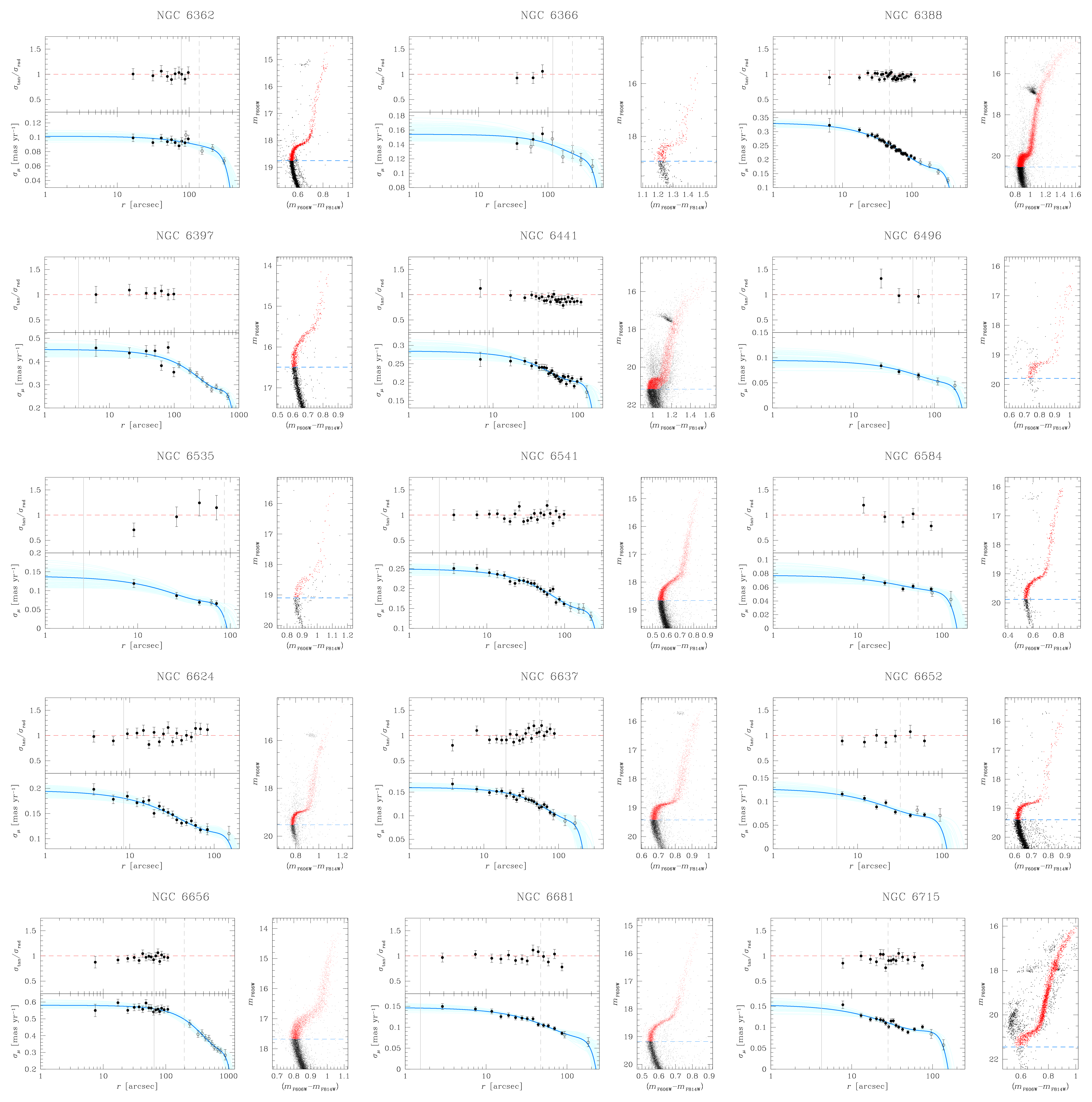
Figure A4: Similar to Figs. A2 and A3, but for NGC 6362, NGC 6366, GC 6388, NGC 6397, NGC 6441, NGC 6496, NGC 6535, NGC 6541, NGC 6584, NGC 6624, NGC 6637, NGC 6652, NGC 6656, NGC 6681 and NGC 6715.

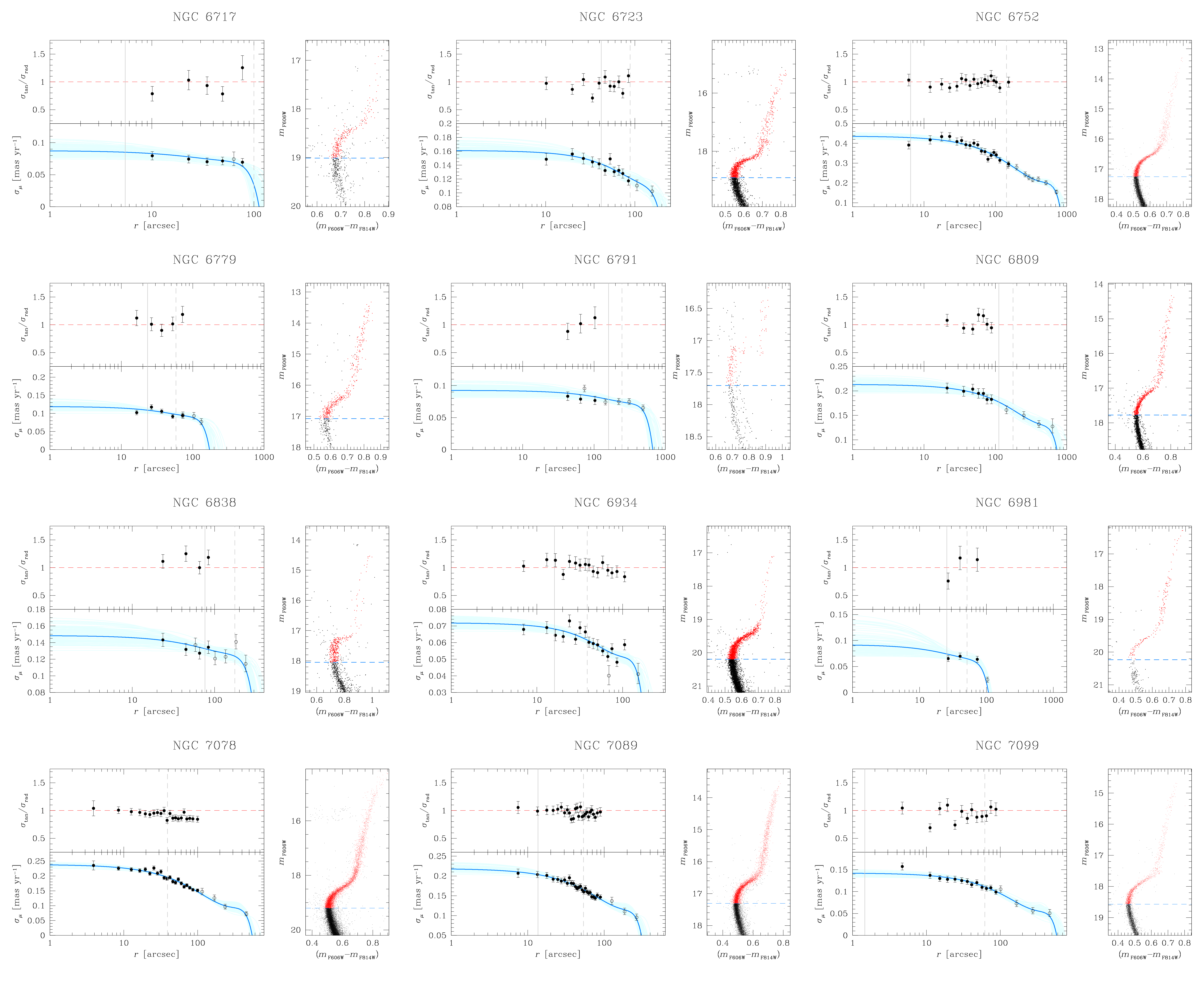
Figure A5: Similar to Figs. A2, A3 and A4, but for NGC 6717, NGC 6723, NGC 6752, NGC 6779, NGC 6791, NGC 6809, NGC 6838, NGC 6934, NGC 6981, NGC 7078, NGC 7078 and NGC 7099.

Table A4: Velocity dispersions at $r=0$ arcsec, $r_{\rm c}$ and $r_{\rm h}$ for all clusters. Not enough data are available to obtain a reliable estimate of the velocity dispersion at large radii for NGC 5053, NGC 6535 and NGC 6717.

Cluster	$\sigma_{\mu}^{r=0}$	$\sigma_{\mu}^{r=r_{\rm c}}$	$\sigma_{\mu}^{r=r_{\rm h}}$	Cluster	$\sigma_{\mu}^{r=0}$	$\sigma_{\mu}^{r=r_{\rm c}}$	$\sigma_{\mu}^{r=r_{\rm h}}$
	$[$mas yr-1$]$	$[$mas yr-1$]$	$[$mas yr-1$]$		$[$mas yr-1$]$	$[$mas yr-1$]$	$[$mas yr-1$]$
NGC 0104	$0.592\pm 0.005$	$0.563\pm 0.004$	$0.473\pm 0.004$	NGC 6352	$0.135\pm 0.006$	$0.125\pm 0.002$	$0.117\pm 0.003$
NGC 0288	$0.073\pm 0.003$	$0.065\pm 0.002$	$0.061\pm 0.002$	NGC 6362	$0.101\pm 0.003$	$0.093\pm 0.002$	$0.088\pm 0.002$
NGC 0362	$0.198\pm 0.005$	$0.194\pm 0.003$	$0.171\pm 0.002$	NGC 6366	$0.154\pm 0.007$	$0.137\pm 0.003$	$0.126\pm 0.005$
NGC 1261	$0.073\pm 0.002$	$0.070\pm 0.001$	$0.061\pm 0.001$	NGC 6388	$0.331\pm 0.006$	$0.316\pm 0.005$	$0.254\pm 0.001$
NGC 1851	$0.163\pm 0.003$	$0.162\pm 0.002$	$0.138\pm 0.001$	NGC 6397	$0.452\pm 0.016$	$0.450\pm 0.015$	$0.356\pm 0.006$
NGC 2298	$0.085\pm 0.005$	$0.081\pm 0.003$	$0.067\pm 0.002$	NGC 6441	$0.285\pm 0.012$	$0.277\pm 0.008$	$0.242\pm 0.003$
NGC 2808	$0.300\pm 0.004$	$0.280\pm 0.003$	$0.243\pm 0.001$	NGC 6496	$0.095\pm 0.009$	$0.067\pm 0.003$	$0.056\pm 0.004$
NGC 3201	$0.194\pm 0.005$	$0.184\pm 0.003$	$0.166\pm 0.003$	NGC 6535	$0.139\pm 0.017$	$0.133\pm 0.014$	-
NGC 4590	$0.082\pm 0.004$	$0.075\pm 0.002$	$0.065\pm 0.002$	NGC 6541	$0.250\pm 0.006$	$0.247\pm 0.006$	$0.188\pm 0.002$
NGC 4833	$0.202\pm 0.007$	$0.185\pm 0.002$	$0.166\pm 0.003$	NGC 6584	$0.078\pm 0.006$	$0.066\pm 0.002$	$0.058\pm 0.002$
NGC 5024	$0.082\pm 0.002$	$0.076\pm 0.001$	$0.065\pm 0.001$	NGC 6624	$0.196\pm 0.006$	$0.181\pm 0.004$	$0.125\pm 0.002$
NGC 5053	$0.049\pm 0.007$	-	-	NGC 6637	$0.160\pm 0.005$	$0.148\pm 0.002$	$0.122\pm 0.002$
NGC 5272	$0.173\pm 0.004$	$0.161\pm 0.002$	$0.142\pm 0.002$	NGC 6652	$0.128\pm 0.007$	$0.116\pm 0.004$	$0.080\pm 0.002$
NGC 5286	$0.211\pm 0.009$	$0.205\pm 0.007$	$0.173\pm 0.003$	NGC 6656	$0.581\pm 0.010$	$0.560\pm 0.005$	$0.496\pm 0.008$
NGC 5466	$0.037\pm 0.003$	$0.029\pm 0.001$	$0.028\pm 0.002$	NGC 6681	$0.147\pm 0.004$	$0.146\pm 0.004$	$0.108\pm 0.002$
NGC 5897	$0.069\pm 0.006$	$0.052\pm 0.002$	$0.048\pm 0.003$	NGC 6715	$0.154\pm 0.007$	$0.145\pm 0.005$	$0.110\pm 0.001$
NGC 5904	$0.213\pm 0.003$	$0.207\pm 0.002$	$0.187\pm 0.003$	NGC 6717	$0.088\pm 0.007$	$0.085\pm 0.006$	-
NGC 5927	$0.157\pm 0.003$	$0.152\pm 0.002$	$0.142\pm 0.002$	NGC 6723	$0.161\pm 0.007$	$0.140\pm 0.003$	$0.120\pm 0.003$
NGC 5986	$0.159\pm 0.005$	$0.149\pm 0.002$	$0.134\pm 0.001$	NGC 6752	$0.436\pm 0.009$	$0.429\pm 0.008$	$0.302\pm 0.005$
NGC 6093	$0.254\pm 0.008$	$0.239\pm 0.006$	$0.199\pm 0.003$	NGC 6779	$0.119\pm 0.008$	$0.108\pm 0.004$	$0.096\pm 0.003$
NGC 6101	$0.058\pm 0.003$	$0.049\pm 0.001$	$0.041\pm 0.004$	NGC 6791	$0.093\pm 0.006$	$0.078\pm 0.002$	$0.074\pm 0.003$
NGC 6121	$0.563\pm 0.015$	$0.552\pm 0.010$	$0.456\pm 0.004$	NGC 6809	$0.213\pm 0.008$	$0.177\pm 0.004$	$0.161\pm 0.004$
NGC 6144	$0.112\pm 0.008$	$0.098\pm 0.003$	$0.090\pm 0.003$	NGC 6838	$0.149\pm 0.008$	$0.132\pm 0.003$	$0.125\pm 0.004$
NGC 6171	$0.143\pm 0.005$	$0.137\pm 0.003$	$0.124\pm 0.003$	NGC 6934	$0.072\pm 0.002$	$0.068\pm 0.001$	$0.061\pm 0.001$
NGC 6205	$0.261\pm 0.006$	$0.233\pm 0.002$	$0.211\pm 0.002$	NGC 6981	$0.092\pm 0.016$	$0.073\pm 0.004$	$0.065\pm 0.004$
NGC 6218	$0.190\pm 0.005$	$0.180\pm 0.003$	$0.163\pm 0.003$	NGC 7078	$0.238\pm 0.003$	$0.237\pm 0.003$	$0.196\pm 0.001$
NGC 6254	$0.260\pm 0.007$	$0.245\pm 0.003$	$0.214\pm 0.004$	NGC 7089	$0.219\pm 0.006$	$0.204\pm 0.003$	$0.166\pm 0.002$
NGC 6304	$0.192\pm 0.006$	$0.190\pm 0.005$	$0.162\pm 0.005$	NGC 7099	$0.143\pm 0.004$	$0.142\pm 0.004$	$0.111\pm 0.002$
NGC 6341	$0.213\pm 0.005$	$0.200\pm 0.003$	$0.174\pm 0.002$

References

- Anderson (2016) Anderson, J. 2016, Empirical Models for the WFC3/IR PSF, Space Telescope WFC Instrument Science Report
- Anderson & Bedin (2010) Anderson, J., & Bedin, L. R. 2010, PASP, 122, 1035, doi: 10.1086/656399
- Anderson & King (2004) Anderson, J., & King, I. R. 2004, Multi-filter PSFs and Distortion Corrections for the HRC, Instrument Science Report ACS 2004-15
- Anderson & King (2006) —. 2006, PSFs, Photometry, and Astronomy for the ACS/WFC, Instrument Science Report ACS 2006-01
- Anderson & van der Marel (2010) Anderson, J., & van der Marel, R. P. 2010, ApJ, 710, 1032, doi: 10.1088/0004-637X/710/2/1032
- Astropy Collaboration et al. (2013) Astropy Collaboration, Robitaille, T. P., Tollerud, E. J., et al. 2013, A&A, 558, A33, doi: 10.1051/0004-6361/201322068
- Astropy Collaboration et al. (2018) Astropy Collaboration, Price-Whelan, A. M., Sipőcz, B. M., et al. 2018, AJ, 156, 123, doi: 10.3847/1538-3881/aabc4f
- Baldwin et al. (2016) Baldwin, A. T., Watkins, L. L., van der Marel, R. P., et al. 2016, ApJ, 827, 12, doi: 10.3847/0004-637X/827/1/12
- Bastian & Lardo (2018) Bastian, N., & Lardo, C. 2018, ARA&A, 56, 83, doi: 10.1146/annurev-astro-081817-051839
- Baumgardt & Vasiliev (2021) Baumgardt, H., & Vasiliev, E. 2021, MNRAS, 505, 5957, doi: 10.1093/mnras/stab1474
- Bedin et al. (2004) Bedin, L. R., Piotto, G., Anderson, J., et al. 2004, ApJ, 605, L125, doi: 10.1086/420847
- Bedin et al. (2019) Bedin, L. R., Salaris, M., Anderson, J., et al. 2019, MNRAS, 488, 3857, doi: 10.1093/mnras/stz1968
- Bekki (2010) Bekki, K. 2010, ApJ, 724, L99, doi: 10.1088/2041-8205/724/1/L99
- Bellini et al. (2011) Bellini, A., Anderson, J., & Bedin, L. R. 2011, PASP, 123, 622, doi: 10.1086/659878
- Bellini et al. (2017a) Bellini, A., Anderson, J., Bedin, L. R., et al. 2017a, ApJ, 842, 6, doi: 10.3847/1538-4357/aa7059
- Bellini & Bedin (2009) Bellini, A., & Bedin, L. R. 2009, PASP, 121, 1419, doi: 10.1086/649061
- Bellini et al. (2017b) Bellini, A., Bianchini, P., Varri, A. L., et al. 2017b, ApJ, 844, 167, doi: 10.3847/1538-4357/aa7c5f
- Bellini et al. (2013) Bellini, A., Piotto, G., Milone, A. P., et al. 2013, ApJ, 765, 32, doi: 10.1088/0004-637X/765/1/32
- Bellini et al. (2014) Bellini, A., Anderson, J., van der Marel, R. P., et al. 2014, ApJ, 797, 115, doi: 10.1088/0004-637X/797/2/115
- Bellini et al. (2015) Bellini, A., Vesperini, E., Piotto, G., et al. 2015, ApJ, 810, L13, doi: 10.1088/2041-8205/810/1/L13
- Bellini et al. (2018) Bellini, A., Libralato, M., Bedin, L. R., et al. 2018, ApJ, 853, 86, doi: 10.3847/1538-4357/aaa3ec
- Bianchini et al. (2017) Bianchini, P., Sills, A., & Miholics, M. 2017, MNRAS, 471, 1181, doi: 10.1093/mnras/stx1680
- Bianchini et al. (2016) Bianchini, P., van de Ven, G., Norris, M. A., Schinnerer, E., & Varri, A. L. 2016, MNRAS, 458, 3644, doi: 10.1093/mnras/stw552
- Bianchini et al. (2018a) Bianchini, P., van der Marel, R. P., del Pino, A., et al. 2018a, MNRAS, 481, 2125, doi: 10.1093/mnras/sty2365
- Bianchini et al. (2018b) Bianchini, P., Webb, J. J., Sills, A., & Vesperini, E. 2018b, MNRAS, 475, L96, doi: 10.1093/mnrasl/sly013
- Binney & Tremaine (2008) Binney, J., & Tremaine, S. 2008, Galactic Dynamics: Second Edition
- Breen et al. (2021) Breen, P. G., Rozier, S., Heggie, D. C., & Varri, A. L. 2021, MNRAS, 502, 4762, doi: 10.1093/mnras/stab365
- Breen et al. (2017) Breen, P. G., Varri, A. L., & Heggie, D. C. 2017, MNRAS, 471, 2778, doi: 10.1093/mnras/stx1750
- Brogaard et al. (2021) Brogaard, K., Grundahl, F., Sandquist, E. L., et al. 2021, A&A, 649, A178, doi: 10.1051/0004-6361/202140911
- Calura et al. (2019) Calura, F., D’Ercole, A., Vesperini, E., Vanzella, E., & Sollima, A. 2019, MNRAS, 489, 3269, doi: 10.1093/mnras/stz2055
- Carretta et al. (2009a) Carretta, E., Bragaglia, A., Gratton, R., & Lucatello, S. 2009a, A&A, 505, 139, doi: 10.1051/0004-6361/200912097
- Carretta et al. (2009b) Carretta, E., Bragaglia, A., Gratton, R. G., et al. 2009b, A&A, 505, 117, doi: 10.1051/0004-6361/200912096
- Cassisi & Salaris (2020) Cassisi, S., & Salaris, M. 2020, A&A Rev., 28, 5, doi: 10.1007/s00159-020-00127-y
- Cohen et al. (2021) Cohen, R. E., Bellini, A., Libralato, M., et al. 2021, AJ, 161, 41, doi: 10.3847/1538-3881/abd036
- Cordoni et al. (2020a) Cordoni, G., Milone, A. P., Mastrobuono-Battisti, A., et al. 2020a, ApJ, 889, 18, doi: 10.3847/1538-4357/ab5aee
- Cordoni et al. (2020b) Cordoni, G., Milone, A. P., Marino, A. F., et al. 2020b, ApJ, 898, 147, doi: 10.3847/1538-4357/aba04b
- Da Costa & Freeman (1976) Da Costa, G. S., & Freeman, K. C. 1976, ApJ, 206, 128, doi: 10.1086/154363
- Dalessandro et al. (2015) Dalessandro, E., Miocchi, P., Carraro, G., Jílková, L., & Moitinho, A. 2015, MNRAS, 449, 1811, doi: 10.1093/mnras/stv395
- Dalessandro et al. (2013) Dalessandro, E., Ferraro, F. R., Massari, D., et al. 2013, ApJ, 778, 135, doi: 10.1088/0004-637X/778/2/135
- Dalessandro et al. (2018a) Dalessandro, E., Cadelano, M., Vesperini, E., et al. 2018a, ApJ, 859, 15, doi: 10.3847/1538-4357/aabb56
- Dalessandro et al. (2018b) Dalessandro, E., Mucciarelli, A., Bellazzini, M., et al. 2018b, ApJ, 864, 33, doi: 10.3847/1538-4357/aad4b3
- Dalessandro et al. (2019) Dalessandro, E., Cadelano, M., Vesperini, E., et al. 2019, ApJ, 884, L24, doi: 10.3847/2041-8213/ab45f7
- Dotter et al. (2010) Dotter, A., Sarajedini, A., Anderson, J., et al. 2010, ApJ, 708, 698, doi: 10.1088/0004-637X/708/1/698
- Evans et al. (2021) Evans, A. J., Strigari, L. E., & Zivick, P. 2021, arXiv e-prints, arXiv:2109.10998. https://arxiv.org/abs/2109.10998
- Ferraro et al. (2018) Ferraro, F. R., Lanzoni, B., Raso, S., et al. 2018, ApJ, 860, 36, doi: 10.3847/1538-4357/aac01c
- Foreman-Mackey et al. (2013) Foreman-Mackey, D., Hogg, D. W., Lang, D., & Goodman, J. 2013, PASP, 125, 306, doi: 10.1086/670067
- Gaia Collaboration et al. (2016) Gaia Collaboration, Prusti, T., de Bruijne, J. H. J., et al. 2016, A&A, 595, A1, doi: 10.1051/0004-6361/201629272
- Gaia Collaboration et al. (2018a) Gaia Collaboration, Katz, D., Antoja, T., et al. 2018a, A&A, 616, A11, doi: 10.1051/0004-6361/201832865
- Gaia Collaboration et al. (2018b) Gaia Collaboration, Brown, A. G. A., Vallenari, A., et al. 2018b, A&A, 616, A1, doi: 10.1051/0004-6361/201833051
- Gieles & Zocchi (2015) Gieles, M., & Zocchi, A. 2015, MNRAS, 454, 576, doi: 10.1093/mnras/stv1848
- Giersz et al. (2013) Giersz, M., Heggie, D. C., Hurley, J. R., & Hypki, A. 2013, MNRAS, 431, 2184, doi: 10.1093/mnras/stt307
- Goldsbury et al. (2010) Goldsbury, R., Richer, H. B., Anderson, J., et al. 2010, AJ, 140, 1830, doi: 10.1088/0004-6256/140/6/1830
- Gontcharov et al. (2019) Gontcharov, G. A., Mosenkov, A. V., & Khovritchev, M. Y. 2019, MNRAS, 483, 4949, doi: 10.1093/mnras/sty3439
- Gratton et al. (2019) Gratton, R., Bragaglia, A., Carretta, E., et al. 2019, A&A Rev., 27, 8, doi: 10.1007/s00159-019-0119-3
- Gratton et al. (2012) Gratton, R. G., Carretta, E., & Bragaglia, A. 2012, A&A Rev., 20, 50, doi: 10.1007/s00159-012-0050-3
- Gratton et al. (2013) Gratton, R. G., Lucatello, S., Sollima, A., et al. 2013, A&A, 549, A41, doi: 10.1051/0004-6361/201219976
- Greene et al. (2020) Greene, J. E., Strader, J., & Ho, L. C. 2020, ARA&A, 58, 257, doi: 10.1146/annurev-astro-032620-021835
- Gunn & Griffin (1979) Gunn, J. E., & Griffin, R. F. 1979, AJ, 84, 752, doi: 10.1086/112477
- Häberle et al. (2021) Häberle, M., Libralato, M., Bellini, A., et al. 2021, MNRAS, 503, 1490, doi: 10.1093/mnras/stab474
- Harris (1996) Harris, W. E. 1996, AJ, 112, 1487, doi: 10.1086/118116
- Hénault-Brunet et al. (2015) Hénault-Brunet, V., Gieles, M., Agertz, O., & Read, J. I. 2015, MNRAS, 450, 1164, doi: 10.1093/mnras/stv675
- Hidalgo et al. (2018) Hidalgo, S. L., Pietrinferni, A., Cassisi, S., et al. 2018, ApJ, 856, 125, doi: 10.3847/1538-4357/aab158
- Holtzman et al. (1995) Holtzman, J. A., Hester, J. J., Casertano, S., et al. 1995, PASP, 107, 156, doi: 10.1086/133533
- Ibata et al. (2021) Ibata, R., Malhan, K., Martin, N., et al. 2021, ApJ, 914, 123, doi: 10.3847/1538-4357/abfcc2
- Ibata et al. (2019) Ibata, R. A., Malhan, K., & Martin, N. F. 2019, ApJ, 872, 152, doi: 10.3847/1538-4357/ab0080
- Ivans et al. (2001) Ivans, I. I., Kraft, R. P., Sneden, C., et al. 2001, AJ, 122, 1438, doi: 10.1086/322108
- Jindal et al. (2019) Jindal, A., Webb, J. J., & Bovy, J. 2019, MNRAS, 487, 3693, doi: 10.1093/mnras/stz1586
- Kamann et al. (2019) Kamann, S., Bastian, N. J., Gieles, M., Balbinot, E., & Hénault-Brunet, V. 2019, MNRAS, 483, 2197, doi: 10.1093/mnras/sty3144
- King (1966) King, I. R. 1966, AJ, 71, 64, doi: 10.1086/109857
- Koch & McWilliam (2014) Koch, A., & McWilliam, A. 2014, A&A, 565, A23, doi: 10.1051/0004-6361/201323119
- Kroupa (2001) Kroupa, P. 2001, MNRAS, 322, 231, doi: 10.1046/j.1365-8711.2001.04022.x
- Lanzoni et al. (2018) Lanzoni, B., Ferraro, F. R., Mucciarelli, A., et al. 2018, ApJ, 861, 16, doi: 10.3847/1538-4357/aac26a
- Lee (2017) Lee, J.-W. 2017, ApJ, 844, 77, doi: 10.3847/1538-4357/aa7b8c
- Lee (2021) —. 2021, ApJ, 918, L24, doi: 10.3847/2041-8213/ac1ffe
- Lee et al. (1999) Lee, Y. W., Joo, J. M., Sohn, Y. J., et al. 1999, Nature, 402, 55, doi: 10.1038/46985
- Libralato et al. (2019) Libralato, M., Bellini, A., Piotto, G., et al. 2019, ApJ, 873, 109, doi: 10.3847/1538-4357/ab0551
- Libralato et al. (2018a) Libralato, M., Bellini, A., van der Marel, R. P., et al. 2018a, ApJ, 861, 99, doi: 10.3847/1538-4357/aac6c0
- Libralato et al. (2018b) Libralato, M., Bellini, A., Bedin, L. R., et al. 2018b, ApJ, 854, 45, doi: 10.3847/1538-4357/aaa59e
- Makino (1996) Makino, J. 1996, ApJ, 471, 796, doi: 10.1086/178007
- Mastrobuono-Battisti & Perets (2013) Mastrobuono-Battisti, A., & Perets, H. B. 2013, ApJ, 779, 85, doi: 10.1088/0004-637X/779/1/85
- Mastrobuono-Battisti & Perets (2016) —. 2016, ApJ, 823, 61, doi: 10.3847/0004-637X/823/1/61
- McLaughlin & van der Marel (2005) McLaughlin, D. E., & van der Marel, R. P. 2005, ApJS, 161, 304, doi: 10.1086/497429
- Milone et al. (2018) Milone, A. P., Marino, A. F., Mastrobuono-Battisti, A., & Lagioia, E. P. 2018, MNRAS, 479, 5005, doi: 10.1093/mnras/sty1873
- Milone et al. (2014) Milone, A. P., Marino, A. F., Dotter, A., et al. 2014, ApJ, 785, 21, doi: 10.1088/0004-637X/785/1/21
- Milone et al. (2017) Milone, A. P., Piotto, G., Renzini, A., et al. 2017, MNRAS, 464, 3636, doi: 10.1093/mnras/stw2531
- Monelli et al. (2013) Monelli, M., Milone, A. P., Stetson, P. B., et al. 2013, MNRAS, 431, 2126, doi: 10.1093/mnras/stt273
- Nardiello et al. (2018) Nardiello, D., Libralato, M., Piotto, G., et al. 2018, MNRAS, 481, 3382, doi: 10.1093/mnras/sty2515
- Noyola & Gebhardt (2006) Noyola, E., & Gebhardt, K. 2006, AJ, 132, 447, doi: 10.1086/505390
- Pancino et al. (2017) Pancino, E., Bellazzini, M., Giuffrida, G., & Marinoni, S. 2017, MNRAS, 467, 412, doi: 10.1093/mnras/stx079
- Pavlík & Vesperini (2021) Pavlík, V., & Vesperini, E. 2021, MNRAS, 504, L12, doi: 10.1093/mnrasl/slab026
- Pavlík & Vesperini (2022) —. 2022, MNRAS, 509, 3815, doi: 10.1093/mnras/stab3157
- Pedregosa et al. (2011) Pedregosa, F., Varoquaux, G., Gramfort, A., et al. 2011, Journal of Machine Learning Research, 12, 2825
- Piotto et al. (2015) Piotto, G., Milone, A. P., Bedin, L. R., et al. 2015, AJ, 149, 91, doi: 10.1088/0004-6256/149/3/91
- Raso et al. (2019) Raso, S., Pallanca, C., Ferraro, F. R., et al. 2019, ApJ, 879, 56, doi: 10.3847/1538-4357/ab2637
- Raso et al. (2020) Raso, S., Libralato, M., Bellini, A., et al. 2020, ApJ, 895, 15, doi: 10.3847/1538-4357/ab8ae7
- Recio-Blanco et al. (2005) Recio-Blanco, A., Piotto, G., de Angeli, F., et al. 2005, A&A, 432, 851, doi: 10.1051/0004-6361:20041053
- Renzini et al. (2015) Renzini, A., D’Antona, F., Cassisi, S., et al. 2015, MNRAS, 454, 4197, doi: 10.1093/mnras/stv2268
- Richer et al. (2013) Richer, H. B., Heyl, J., Anderson, J., et al. 2013, ApJ, 771, L15, doi: 10.1088/2041-8205/771/1/L15
- Rossi et al. (2015) Rossi, L. J., Ortolani, S., Barbuy, B., Bica, E., & Bonfanti, A. 2015, MNRAS, 450, 3270, doi: 10.1093/mnras/stv748
- Sollima (2021) Sollima, A. 2021, MNRAS, 502, 1974, doi: 10.1093/mnras/stab154
- Spitzer (1987) Spitzer, L. 1987, Dynamical evolution of globular clusters
- Szölgyén et al. (2019) Szölgyén, Á., Meiron, Y., & Kocsis, B. 2019, ApJ, 887, 123, doi: 10.3847/1538-4357/ab50bb
- Tiongco et al. (2016a) Tiongco, M. A., Vesperini, E., & Varri, A. L. 2016a, MNRAS, 461, 402, doi: 10.1093/mnras/stw1341
- Tiongco et al. (2016b) —. 2016b, MNRAS, 455, 3693, doi: 10.1093/mnras/stv2574
- Tiongco et al. (2017) —. 2017, MNRAS, 469, 683, doi: 10.1093/mnras/stx853
- Tiongco et al. (2018) —. 2018, MNRAS, 475, L86, doi: 10.1093/mnrasl/sly009
- Tiongco et al. (2019) —. 2019, MNRAS, 487, 5535, doi: 10.1093/mnras/stz1595
- Trager et al. (1995) Trager, S. C., King, I. R., & Djorgovski, S. 1995, AJ, 109, 218, doi: 10.1086/117268
- Trenti & van der Marel (2013) Trenti, M., & van der Marel, R. 2013, MNRAS, 435, 3272, doi: 10.1093/mnras/stt1521
- van de Ven et al. (2006) van de Ven, G., van den Bosch, R. C. E., Verolme, E. K., & de Zeeuw, P. T. 2006, A&A, 445, 513, doi: 10.1051/0004-6361:20053061
- Varri et al. (2018) Varri, A. L., Cai, M. X., Concha-Ramírez, F., et al. 2018, Computational Astrophysics and Cosmology, 5, 2, doi: 10.1186/s40668-018-0024-6