Withholding Verifiable Information

Abstract

I study a class of verifiable disclosure games where the sender’s payoff is state independent and the receiver’s optimal action only depends on the expected state. The sender’s messages are verifiable in the sense that they can be vague but can never be wrong. What is the sender’s preferred equilibrium? When does the sender gain nothing from having commitment power? I identify conditions for an information design outcome to be an equilibrium outcome of the verifiable disclosure game, and give simple sufficient conditions under which the sender does not benefit from commitment power. These results help in characterizing the sender’s preferred equilibria and her equilibrium payoff set in a class of verifiable disclosure games. I apply these insights to study influencing voters and selling with quality disclosure.

Keywords: Communication, Verifiable disclosure games, Sender’s preferred equilibrium, Information design
JEL Classifications: C72; D82; D83

1 Introduction

In many economic interactions that involve communication between a sender and a receiver, the sender’s messages are verifiable in the sense that they can be vague but can never be false. Examples include sellers disclosing and highlighting certain features of a product to consumers, political experts organizing and simplifying poll results for politicians, and advisors condensing and distilling market research for their managers. In each of these examples, if the sender releases information that is inherently false, she would face severe consequences: a seller might be sued for compensation, and an expert or advisor could be fired for lying.

I study a communication game in which the sender’s messages are verifiable, a so-called verifiable disclosure game, and emphasize the extent to which the sender benefits from communication. It is well known that the unraveling equilibria, in which the sender’s private information is fully revealed, are the receiver’s preferred equilibria (Grossman, 1981; Milgrom, 1981). However, little is known about the sender’s preferred equilibria. How much can the sender benefit from verifiable communication? What are the structures of the sender’s preferred equilibria?

In this paper, I find conditions under which the sender’s payoff in her preferred equilibrium is the same as if she could commit to an arbitrary information structure. Then I develop tools to characterize the sender’s preferred equilibrium if these conditions are not satisfied. I also discuss other equilibria of the game as well as the sender’s equilibrium payoff set. Applications discuss how a seller should optimally reveal product information and how an expert should communicate with voters.

In the model, there is a one-dimensional state of the world that is payoff-relevant to the receiver and only observable to the sender. The sender sends a message, and the receiver subsequently chooses an action from a finite set. The actions are “ordered” in the sense that the receiver would like to use a higher action when the expected state is higher, and the sender strictly prefers a higher action regardless of the state. Verifiability requires that the sender’s messages must contain the true state. Finally, the sender’s payoff depends only on the receiver’s action (in jargon, the sender’s preferences are state-independent), and the receiver’s optimal choice of action depends only on the expected state.

A natural upper bound of the sender’s expected payoff in the sender’s preferred equilibrium is given by the solution to the corresponding information design problem. The information design approach, popularized by Kamenica and Gentzkow (2011), assumes that the sender has commitment power: she can commit to any information structure that reveals information about the state. Kleiner, Moldovanu, and Strack (2021) and Arieli, Babichenko, Smorodinsky, and Yamashita (2022) show that every information design problem admits a salient solution, a so-called bi-pooling solution, that has a simple structure and is easy to identify. If a bi-pooling solution can be induced by an equilibrium, it must be a sender’s preferred equilibrium, and the sender’s payoff in this equilibrium coincides with the commitment payoff.

My first set of results identifies necessary and sufficient conditions under which a bi-pooling solution is an equilibrium outcome of the verifiable disclosure game. These results suggest a “guess and verify” approach for finding the sender’s preferred equilibrium: one can solve the corresponding information design problem first, and then check whether the conditions hold. I first note that every bi-pooling solution can be represented by a partition of the state space such that the same action is recommended in all states belonging to the same partitional element. Furthermore, each partitional element is either an interval or obtained from “subtracting” an interval from a larger interval. Among other things, I find that a bi-pooling solution is an equilibrium outcome if and only if in each state the sender prefers to use the partitional element that contains the state as her message rather than fully disclose the state.

My second set of results provides sufficient conditions on model primitives under which commitment has no value; i.e., that imply the commitment payoff can be achieved in an equilibrium. The first condition requires that it is sufficiently more profitable for the sender to induce the higher action than the lower one for any pair of adjacent actions, which guarantees that it is never optimal for the sender to recommend a lower action in a state in which a higher action is optimal. Another sufficient condition, which is implied by the first one, identifies separate conditions on the prior distribution and the sender’s value function. Importantly, under any of these conditions, the sender’s preferred equilibrium of a verifiable disclosure game can be obtained by solving the corresponding information design problem. Moreover, for any information design problem that satisfies one of these conditions, the commitment assumption can be dispensed with.

Even if the commitment payoff cannot be attained in any equilibrium, I show that the sender’s preferred equilibrium exists, and I characterize its properties. In particular, in this equilibrium, every on-path message of the sender can be interpreted as an action recommendation that the receiver finds optimal to follow, and the messages have a simple structure. Furthermore, the sender’s expected payoff in this equilibrium is strictly higher than the unraveling payoff. In the special case that the receiver has three actions, I explicitly solve the sender’s preferred equilibrium. Moreover, I find that any payoff that is below the sender’s payoff in her preferred equilibrium and above the unraveling payoff can be sustained in an equilibrium in which the on-path messages have the properties described above.

I apply these insights to study selling with information disclosure and influencing voters. In the selling setting, Milgrom (1981) shows that when the buyer can buy any fraction of the product, every equilibrium of the game features unraveling. Perhaps surprisingly, if the buyer is restricted to buying integer units, the seller may be able to achieve the same outcome as if she has commitment power. Next, I consider an expert who discloses verifiable information to a group of voters in an amendment voting setting; that is, voters choose from one of the three alternatives: the amended bill, the (unamended) bill, and no bill (or status quo). Interestingly, the expert can be hurt even if, all else equal, all voters are more inclined toward the expert’s most preferred outcome.

Finally, I consider two extensions of the baseline model: in one of them I allow the state to be multidimensional, and in another I drop the “orderedness” of actions and further allow the receiver’s action space to be an interval. For both extensions, I find necessary and sufficient conditions under which a bi-pooling solution (or, when the state is multidimensional, its natural generalization) is an equilibrium outcome. I also identify economically meaningful communication environments in which either commitment has no value, or the commitment payoff cannot be obtained in any equilibrium.

Related literature.

As mentioned above, the study of verifiable disclosure games initiated from Grossman and Hart (1980), Grossman (1981), and Milgrom (1981); for surveys of this literature, see Milgrom (2008) and Dranove and Jin (2010). As far as I know, there are very few papers studying the sender’s preferred equilibria in verifiable disclosure games. Ali, Lewis, and Vasserman (2022) consider a model of personalized pricing with disclosure of verifiable payoff-relevant information by a consumer, and they study the highest consumer surplus that can be achieved in equilibrium under different assumptions on the consumer’s message space. Closest to mine is Titova (2022): she shows that the sender can attain the information design payoff in an equilibrium of the verifiable disclosure game when there are two actions. Titova also assumes that the sender has state-independent preferences, and her assumptions on state space and message space are essentially the same as mine. But she allows that the receiver’s actions are “unordered”, and her result continues to hold when there is more than one receiver given that there is no strategic interaction between receivers.

This work is also connected to the literature on the sender’s preferred equilibria in cheap talk games. Assuming that the sender has state-independent preferences, Lipnowski and Ravid (2020) characterizes the set of equilibrium payoffs in a cheap talk game, and they show that the sender’s preferred equilibrium payoff is given by the quasiconcave hull of the sender’s value function evaluated at the prior. Lipnowski (2020) shows that in a cheap talk game with finite parameters, a sufficient condition for the sender to attain the same payoff as under communication with commitment is that her value function is continuous.

Finally, this paper is related to the literature on relaxing the commitment assumption in information design problems. Lipnowski, Ravid, and Shishkin (2021) and Min (2021) allow the sender to stochastically and costlessly alter her message after observing the state. In Nguyen and Tan (2021), the sender can costly distort the messages produced by the information structure she chooses. Lin and Liu (2022) consider a sender who can secretly deviate to some other information structures so long as the distribution over messages is the same as the announced one. My model differs in that the only constraint that the sender faces is that her messages have to be verifiable.

2 The Model

There are two players, Sender and Receiver. The state space is $\Omega=[0,1]$, and Sender and Receiver share a common prior $F$, which admits a strictly positive density $f$. Let $\mu_{F}$ denote the probability measure induced by $F$. I assume that Receiver’s optimal action only depends on the posterior mean of the state, denoted by $x$. Receiver has $n<\infty$ actions, and hence her action space is $\mathcal{A}=\{a_{0},a_{1},\ldots,a_{n-1}\}$. There exist cutoffs $0=\gamma_{0}\leq\gamma_{1}\leq\cdots\leq\gamma_{n}=1$ such that $a_{i}$ is optimal if and only if $x\in A_{i}:=[\gamma_{i},\gamma_{i+1}]$. Sender’s payoff $v:\mathcal{A}\to\mathbb{R}$ only depends on Receiver’s action; normalize $v(a_{0})=0$, and assume $v(a_{k})>v(a_{l})$ whenever $k>l$.

Sender observes the state and sends a message to Receiver. Assume that for every $\omega\in[0,1]$, Sender’s message space is $\mathcal{M}(\omega)=\{m\in\mathcal{C}:\omega\in m\}$, where $\mathcal{C}$ denotes the collection of nonempty closed subsets of $[0,1]$. In this setting Sender and Receiver play a verifiable disclosure game, first studied by Grossman and Hart (1980), Grossman (1981), and Milgrom (1981); Sender’s message space in my problem is also identical to the aforementioned papers. Any message is verifiable in the sense that it contains the true state. For each state $\omega\in[0,1]$, the assumption on message space allows Sender to fully reveal the state, namely sending $m=\{\omega\}$, or to disclose nothing, that is sending $m=[0,1]$.

Formally, the verifiable disclosure game is defined as follows. Sender’s strategy set, $\Sigma$, is the set of functions $\sigma:[0,1]\to\Delta(\mathcal{C})$ such that $\sigma(\omega)$ is supported on $\mathcal{M}(\omega)$ for each $\omega\in[0,1]$. That is, if Sender uses message $m$ with positive probability in state $\omega$, then it must be that $m$ is feasible in this state. Receiver’s strategy set, $T$, is the set of functions $\tau:\mathcal{C}\to\Delta(\mathcal{A})$. A belief system for Receiver, $p:\mathcal{C}\to\Delta([0,1])$, yielding Receiver’s beliefs about the state as a function of the observed message.

Say that $(\sigma,\tau,p)$ is a (perfect Bayesian) equilibrium if the following conditions hold. First, $\sigma(\omega)$ is supported on $\operatorname*{arg\,max}_{m^{\prime}\in\mathcal{M}(\omega)}v(\tau(m^{\prime}))$. Second, for every $m\in\mathcal{C}$ and $a_{i}\in\mathcal{A}$, $\tau(a_{i}\,|\,m)>0$ implies $\mathbb{E}[\omega\mid\omega\in m]\in[\gamma_{i},\gamma_{i+1}]$. Third, for every $\omega\in[0,1]$ and $m\in\mathcal{C}$, $\omega\not\in\operatorname{supp}{(p(m))}$ if $m\not\in\mathcal{M}(\omega)$. That is, Receiver must deem any state in which the observed message $m$ cannot be sent impossible. Finally, $p$ is obtained from the prior $F$, given $\sigma$, using Bayes’ rule. An outcome of this verifiable disclosure game is a pair $(G,R)\in\Delta([0,1])\times\mathbb{R}$, where $G$ is the induced distribution over Receiver’s posterior means, and $R$ is Sender’s ex ante payoff. An outcome is an equilibrium outcome if it is induced by an equilibrium.

A bulk of this paper concerns Sender’s preferred equilibria of this verifiable disclosure game, which are the equilibria that attain the highest possible Sender’s ex ante payoff. For this purpose, it is useful to introduce Sender’s value function $u:[0,1]\rightarrow\mathbb{R}$, which maps every posterior mean $x$ to the highest attainable expected Sender payoff, conditional on the posterior mean being $x$ and Receiver choosing her optimal action. Figure 1 illustrates Sender’s value function when there are four actions. By definition, $u(x)$ is constant on $(\gamma_{i},\gamma_{i+1})$ has discontinuous at $\gamma_{i}$ for each $i=1,2,\ldots,n-1$. Moreover, it is upper semicontinuous.

Figure 1: An illustration for Sender’s value function, which is a function of posterior mean $x$, when there are four actions.

To study Sender’s preferred equilibria and the value of commitment, I also consider the information design problem based on this communication environment as a benchmark. In this problem, Sender can commit to any experiment that reveals information about the state. An experiment $(\chi,S)$ consists of a signal space $S$ and a mapping $\chi:[0,1]\to\Delta(S)$; an experiment induces a signal distribution in $\Delta(S)$. For each state $\omega\in[0,1]$, $\chi(\omega)$ identifies a distribution over signal space $S$; an experiment is deterministic if $\chi(\omega)$ is a degenerate distribution for each $\omega\in[0,1]$. And because Receiver’s optimal action only depends on the posterior mean of the state, it is without loss to restrict attention on the class of experiments where $S=[0,1]$, and each $s\in S$ equals the induced posterior mean: $s=\mathbb{E}[\omega\,|\,s]$. It is well known that a signal distribution $G$ is induced by an experiment if and only if $G$ is a mean-preserving contraction of $F$; consequently, Sender’s problem is to choose a posterior mean distribution that solves

$$\max_{G\in\text{MPC}(F)}\int_{0}^{1}u(x)\,\mathrm{d}G(x),$$ (1)

where $\text{MPC}(F)$ is the set of mean-preserving contractions of $F$. I call any solution $G_{c}$ to problem 1 an optimal signal distribution, and call the value of problem 1, denoted by $R_{c}$, the commitment payoff. Clearly, $R_{c}$ is an upper bound of Sender’s equilibrium payoff in the verifiable disclosure game.

Say that a pair $(G,R)\in\Delta([0,1])\times\mathbb{R}$ is a commitment outcome if $G$ is an optimal signal distribution and $R$ is Sender’s commitment payoff. A commitment outcome $(G,R)$ is implementable by verifiable messages, or just implementable for short, if $(G,R)$ is an equilibrium outcome of the verifiable disclosure game based on the same communication environment. I usually abuse notation and say that an optimal signal distribution $G$ is implementable when the commitment outcome it induces is implementable.

3 Implementability

There are two sets of results presented in this section. The first set of results (Section 3.3) provides necessary and sufficient conditions under which a particular commitment outcome can be implemented. And the second set of results (Section 3.4) provides sufficient conditions on model primitives under which commitment has no value. To get there, I first characterize a salient class of solutions to the information design problem; this is handled in Section 3.1 and Section 3.2.

3.1 Characterizing Information Design Solution

I start by introducing a class of simple signal distributions.

Definition 1 (Bi-pooling distribution).

A distribution $G\in\text{MPC}(F)$ is a bi-pooling distribution if there exists a collection of pairwise disjoint intervals $\left\{\left[\underline{\omega}_{i},\overline{\omega}_{i}\right]\right\}_{i\in\mathcal{I}}$ such that

• for all $i\in\mathcal{I}$, $G\left(\overline{\omega}_{i}\right)-G\left(\underline{\omega}_{i}\right)=F\left(\overline{\omega}_{i}\right)-F\left(\underline{\omega}_{i}\right)$ and $\left|\operatorname{supp}\left(G|_{[\underline{\omega}_{i},\overline{\omega}_{i}]}\right)\right|\leq 2$;

• $\left.G\right|_{[0,1]\backslash\cup_{i\in\mathcal{I}}\left[\underline{\omega}_{i},\overline{\omega}_{i}\right]}=\left.F\right|_{[0,1]\backslash\cup_{i\in\mathcal{I}}\left[\underline{\omega}_{i},\overline{\omega}_{i}\right]}$.

Intuitively, a bi-pooling distribution partitions the state space in intervals such that in each of them,

• either all states are fully revealed,

• or a single deterministic signal is sent for all states,

• or two different, possibly random, signals are sent.

In particular, $\left[\underline{\omega}_{i},\overline{\omega}_{i}\right]$ is called a pooling interval if $\left|\operatorname{supp}\left(G|_{[\underline{\omega}_{i},\overline{\omega}_{i}]}\right)\right|=1$ (which corresponds to case (ii) above), and it is called a bi-pooling interval if $\left|\operatorname{supp}\left(G|_{[\underline{\omega}_{i},\overline{\omega}_{i}]}\right)\right|=2$ (which corresponds to case (iii) above).

Kleiner et al. (2021) and Arieli et al. (2022) show that every extreme point of $\text{MPC}(F)$ is a bi-pooling distribution. Then because $\text{MPC}(F)$ is convex and compact, and the objective function in problem 1 is linear and upper semicontinuous, by the Bauer’s Maximum Principle, an extreme point of $\text{MPC}(F)$ solves problem 1. Calling a bi-pooling distribution $G_{B}$ that solves the information design problem 1 a bi-pooling solution,

Theorem 3.1 (Kleiner et al. 2021; Arieli et al. 2022).

The information design problem admits a bi-pooling solution.

Applying Theorem 3.1 to my setting, Lemma 3.2 characterizes the optimal signal distribution of Sender’s problem when she has commitment power.

Lemma 3.2 (Candogan, 2019).

Every bi-pooling solution to the information design problem satisfies $\operatorname{supp}{(G_{B})}\subseteq\left[0,\tilde{\gamma}\right]\cup\left\{\gamma_{i}\right\}_{i=1}^{n-1}$, where $\tilde{\gamma}\in[0,1]$ is such that $\tilde{\gamma}\leq\gamma$ for all $\gamma\in\operatorname{supp}{(G_{B})}\cap\left\{\gamma_{i}\right\}_{i=1}^{n-1}$.

An important consequence of Lemma 3.2 is that every signal realization can be interpreted as a recommended action. In particular, every $x\in\operatorname{supp}{(G_{B})}\cap[0,\tilde{\gamma}]$ recommends the “lowest” action, and $\gamma_{i}$ is a recommendation of action $a_{i}$ for each $i=1,2,\ldots,n-1$. Another appealing property of bi-pooling solutions is that they can be solved via a finite-dimensional convex program proposed by Candogan (2019), which admits a polynomial algorithm.

3.2 Deterministic Representations of a Bi-Pooling Solution

It is tempting to ask whether every bi-pooling solution can be induced by a deterministic experiment. To answer this, I introduce some notation first. Say that a bi-pooling interval $[\underline{\omega},\overline{\omega}]$ of a bi-pooling solution $G_{B}$ with $\operatorname{supp}\left(G_{B}|_{[\underline{\omega},\overline{\omega}]}\right)=\{z_{L},z_{H}\}$ where $z_{L}\leq z_{H}$ admits a bi-partition $\{B_{L},B_{H}\}$ if there exist two closed sets $B_{L}$ and $B_{H}$, such that

• $B_{L}\cup B_{H}=[\underline{\omega},\overline{\omega}]$;

• $\mu_{F}\left(B_{L}\cap B_{H}\right)=0$;

• $\mathbb{E}[\omega\mid\omega\in B_{L}]=z_{L}$, and $\mathbb{E}[\omega\mid\omega\in B_{H}]=z_{H}$.

If a bi-pooling interval of a bi-pooling solution admits a bi-partition $\{B_{L},B_{H}\}$, then for $i=H,L$ and every $\omega\in\operatorname{int}{(B_{i})}$, $\mathrm{supp}\,\left(\chi(\omega)\right)=\{z_{i}\}$. In words, in every state that belongs to a component of the bi-partition, a deterministic signal, which is the conditional mean of the state on that component, is realized with probability one.

If each of the bi-pooling intervals admits a bi-partition, by Lemma 3.2, a bi-pooling solution $G_{B}$ can be represented by a sequence of closed sets $\{B_{i}\}_{i=0}^{n-1}$ such that

• $\cup_{i=0}^{n-1}B_{i}=[0,1]$;

• $\mu_{F}\left(B_{i}\cap B_{j}\right)=0$ for any $i,j=0,\ldots,n-1$; and

• if let $j=\min\{i:\operatorname{int}{(B_{i})}\neq\varnothing\}$, then $\mathbb{E}[\omega\mid\omega\in B_{j}]\geq\gamma_{j}$ and $\mathbb{E}[\omega\mid\omega\in B_{i}]=\gamma_{i}$ for all $i>j$.

Then for every $i=0,\ldots,n-1$, $B_{i}\backslash(\cup_{j>i}B_{j})$ is the set of states in which action $a_{i}$ is recommended with probability one; and by (III), every recommendation is obedient in the sense that the receiver’s optimal action coincides with the action recommendation. Say that this bi-pooling solution admits a deterministic representation $\{B_{i}\}_{i=0}^{n-1}$.

Lemma 3.3, which is largely based on Lemma 4 in Arieli et al. (2022), shows that every bi-pooling solution has a particular deterministic representation. Say that a bi-partition $\{B_{L},B_{H}\}$ of a bi-pooling interval $[\underline{\omega},\overline{\omega}]$ is a nested intervals representation if there exist $\underline{b}_{L},\overline{b}_{L}\in[\underline{\omega},\overline{\omega}]$ such that $B_{L}=[\underline{b}_{L},\overline{b}_{L}]$ and $B_{H}=[\underline{\omega},\underline{b}_{L}]\cup[\overline{b}_{L},\overline{\omega}]$.

Lemma 3.3.

Let $[\underline{\omega},\overline{\omega}]$ be a bi-pooling interval of a bi-pooling solution $G$ with $\operatorname{supp}\left(G\,|_{[\underline{\omega},\overline{\omega}]}\right)=\{\gamma_{L},\gamma_{H}\}$ where $\gamma_{L}<\gamma_{H}$, there exists a unique nested interval representation $\{B_{L},B_{H}\}$ of $[\underline{\omega},\overline{\omega}]$.

Unless otherwise noted, the proofs are collected in Appendix A. With the help of Lemma 3.3, a bi-pooling solution can be represented by a deterministic representation $\{B_{i}\}_{i=0}^{n-1}$, where for $i=1,\ldots,n-1$, if $\operatorname{int}{(B_{i})}\neq\varnothing$, $B_{i}$ is either an interval or the union of two intervals. I call such a deterministic representation of a bi-pooling solution a canonical representation; uniqueness of the nested interval representation of bi-pooling intervals begets the essential uniqueness of the canonical representation.

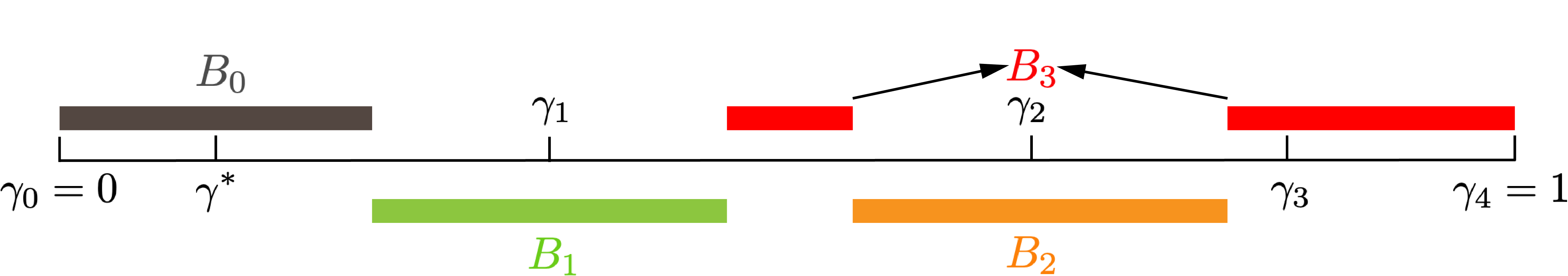
Figure 2: A deterministic representation (upper panel) and a canonical representation (lower panel) of a bi-pooling solution when there are four actions. In the canonical representation displayed in the lower panel, $\{B_{2},B_{3}\}$ is a nested interval representation.

3.3 Characterizing Implementability

The first set of main results characterizes the implementability of any bi-pooling solution.

Definition 2.

A deterministic representation $\{B_{i}\}_{i=0}^{n-1}$ is incentive compatible if deviating to full disclosure is never profitable:

$$A_{i}\subseteq\bigcup_{j=i}^{n-1}B_{j}$$ (IC)

for all $i=0,1,\ldots,n-1$.

To understand IC, consider any state $\omega\in A_{i}$. In this state, Receiver would take action $a_{i}$ under complete information, that is, when the state is fully revealed. But since $A_{i}\subseteq\cup_{j\geq i}B_{j}$, in state $\omega$ the deterministic representation recommends an action at least as preferred as $a_{i}$ with probability one, and Receiver obeys this recommendation. Consequently, deviating to full disclosure is never profitable.

Proposition 3.4.

A bi-pooling solution is implementable if and only if its canonical representation $\{B_{i}\}_{i=0}^{n-1}$ is incentive compatible.

Proposition 3.4 says that to check whether a bi-pooling solution is implementable, it suffices to find its (essentially unique) canonical representation, and see if Condition IC is satisfied. This result is useful because one only needs to focus on a specific messaging strategy of Sender, and only one kind of deviation needs to be considered, namely deviating to full disclosure.

Proposition 3.4 is proved in three steps. As the first step, I show that every implementable bi-pooling solution can be induced by an equilibrium in which both players only use pure strategies. To see this, note that because Receiver only mixes between two adjacent actions, if in a state Sender uses two distinct messages, it must be that they induce the same distribution over Receiver’s actions upon receiving the messages. Therefore, in any state, one can “merge” the multiple messages used with positive probability into one by taking the union. And on Receiver’s side, recall that the commitment payoff is an upper bound of the equilibrium payoff set. Hence, in any equilibrium whose outcome coincides with the commitment outcome Receiver must always break ties in favor of Sender whenever she is indifferent. Consequently, in this equilibrium, every state maps to a single action with probability 1, and hence it can be identified by a deterministic representation.

In the second step, I show that a bi-pooling solution is implementable if and only if there exists a deterministic representation of it that is incentive compatible. The “only if” direction is an immediate consequence of the first step: if a bi-pooling solution is implementable, its outcome is achieved in an equilibrium that can be identified by a deterministic representation. Then it must be that Sender does not want to deviate to full disclosure in any state, and thus the associated deterministic representation must satisfy Condition IC. For the other direction, it suffices to show that for the incentive compatible deterministic representation $\{B_{i}\}_{i=0}^{n-1}$, Sender’s strategy $\sigma$ given by $\sigma(B_{i}\,|\,\omega)=1$ for all $\omega\in B_{i}\backslash(\cup_{j>i}B_{j})$ can be sustained in an equilibrium. To this end, consider the maximally skeptical beliefs: for any off-path message $m\notin\{B_{i}\}_{i=0}^{n-1}$, $p(\min m\,|\,m)=1$. In words, Receiver believes that the state is the lowest possible one when she sees an off-path message. Then because each message must contain the true state, any off-path message is no better than full disclosure. Therefore, Condition IC is also sufficient.

Finally, I show that the canonical representation is the most “deviation proof” one amongst all deterministic representations, in the sense that if a deterministic representation is implementable, the (essentially unique) canonical representation of the same bi-pooling solution is also implementable. Intuitively, suppose $\{\gamma_{L},\gamma_{H}\}$ is bi-pooled to $[\underline{\omega},\overline{\omega}]$; in the canonical representation, $B_{L}$ is the most “concentrated around” $\gamma_{L}$ amongst all deterministic representations, and hence minimizes the chance of $B_{L}$ intersecting $A_{j}$’s with $j\geq L$.

The following result goes one step further: it reveals the exact features of the canonical representation that make Condition IC fail and hence prevent the bi-pooling solution from being implementable. Say that an action $a_{i}$ with $i\geq 1$ is skipped in a deterministic representation $\{B_{i}\}_{i=0}^{n-1}$ if $\operatorname{int}{(B_{i})}=\varnothing$. That is, from an ex ante perspective, this action is recommended with probability zero. And for each action $i$ that is not skipped, let $\bar{b}_{i}=\sup B_{i}$, and $\underline{b}_{i}=\inf B_{i}$.

Proposition 3.5.

A bi-pooling solution is implementable if and only if its canonical representation is such that

• for $i\geq 1$, if $a_{i}$ is skipped, $\overline{b}_{j}\leq\gamma_{i}$ for every unskipped action $a_{j}$ with $j<i$, and

• for every nested intervals representation $\{B_{L},B_{H}\}$, $\overline{b}_{L}\leq\gamma_{H}$.

Figure 3: Violation of the conditions in Proposition 3.5: in the left panel condition (i) is violated because $a_{2}$ is skipped, but $\gamma_{2}<\overline{b}_{1}$ where $a_{1}$ is a “lower” action that is not skipped; in the right panel condition (ii) is violated since $\{B_{2},B_{3}\}$ is a nested intervals representation, but $\overline{b}_{2}>\gamma_{3}$.

For the canonical representation of an arbitrary bi-pooling solution, Condition (i) says that if action $a_{i}$ is skipped, it must be that no “lower” action is recommended in any state in which $a_{i}$ is optimal under complete information. Condition (ii) states that if two unskipped actions, $a_{L}$ and $a_{H}$ with $L<H$, are such that $\{B_{L},B_{H}\}$ is a nested interval representation, then the highest state in which the lower action $a_{L}$ is recommended lies “below” the lowest state in which the higher action $a_{H}$ is optimal under complete information. It is easy to see that Conditions (i) and (ii) are necessary: if any of them is violated, Sender prefers to deviate to full disclosure in a set of states of positive measure. And the special structure of the canonical representation of a bi-pooling solution guarantees that the two conditions are also sufficient for Sender not to deviate to full disclosure in any state. Therefore, the two conditions are equivalent to Condition IC.

An important implication of Proposition 3.5 is that deviating to full disclosure is profitable only when an action $a_{i}$ with $i<n-1$ is induced “too frequently” in the canonical representation; this is illustrated in Figure 3. Furthermore, this “threat” is only relevant for skipped actions and nested intervals. The two conditions in Proposition 3.5 are easier to check than Condition IC in determining whether a bi-pooling solution is implementable, and they allow me to identify sufficient conditions under which commitment has no value in the next subsection.

Corollary 3.6, which is a direct consequence of Proposition 3.5, concerns the special case that there are two actions.

Corollary 3.6.

If $|\mathcal{A}|=2$, then every bi-pooling solution can be implemented.

Corollary 3.6 is very similar to Theorem 2 in Titova (2022). Intuitively, in an information design problem with two actions, Sender’s lone objective is to maximize the probability that the “high action” is played, and hence she only needs to pool as many low states (states in $A_{0}$) with high states (states in $A_{1}$) as possible. Therefore, for all type $\omega\in A_{1}$, it must be that $\omega\in B_{1}$. Consequently, incentive compatibility holds for the (essentially unique) canonical representation of every bi-pooling solution, and hence they are implementable.

In the following example, taken from Gentzkow and Kamenica (2016), the two conditions in Proposition 3.5 are satisfied, and the commitment outcome is hence implementable.

Example 1 (Gentzkow and Kamenica, 2016).

Suppose $\mathcal{A}=\{a_{0},a_{1},a_{2}\}$, and $\gamma_{1}=1/3$, $\gamma_{2}=2/3$; that is,

$$A_{0}=[0,1/3],~{}A_{1}=[1/3,2/3],\text{ and }A_{2}=[2/3,1].$$

The prior $F$ is uniform. Assume also that $v(a_{1})=1$ and $v(a_{2})=3$. Gentzkow and Kamenica (2016) show that

$$B_{0}=\left[0,8/48\right],~{}B_{1}=\left[11/48,21/48\right],~{}B_{2}=\left[8/48,11/48\right]\cup\left[21/48,1\right]$$

is the canonical representation of a bi-pooling solution to the information design problem. Because no action is skipped, and the nested intervals representation $\{B_{1},B_{2}\}$ satisfies $\overline{b}_{1}\leq\gamma_{2}$, by Proposition 3.5, this bi-pooling solution can be implemented. Consequently, Sender’s commitment payoff can be attained in an equilibrium of the verifiable disclosure game.

Example 2 and Example 3 illustrate that for any bi-pooling solution, if one of the conditions in Proposition 3.5 fails to hold, it cannot be implemented. In particular, these examples are obtained by “slightly perturbing” the binary actions environment.

Example 2.

Suppose $\mathcal{A}=\{a_{0},a_{1},a_{2}\}$, and $\gamma_{1}=0.5$, $\gamma_{2}=0.9$; that is,

$$A_{0}=[0,0.5],~{}A_{1}=[0.5,0.9],\text{ and }A_{2}=[0.9,1].$$

The prior $F$ is uniform. Assume that $v(a_{1})=1$ and $v(a_{2})=1.1$. The unique solution to the information design problem has an essentially unique canonical representation $\{B_{0},B_{1},B_{2}\}$ with $B_{1}=[0,1]$ and $B_{0}=B_{2}=\varnothing$. Action $a_{2}$ is skipped, and $0.9=\gamma_{2}<\bar{b}_{1}=1$, which violates Condition (i) in Proposition 3.5. Therefore, this bi-pooling solution cannot be implemented.

When there are three actions, as pointed out by Gentzkow and Kamenica (2016), in the information design problem Sender needs to trade-off between how frequently $a_{1}$ and $a_{2}$ are taken: inducing $a_{2}$ more frequently decreases the frequency that $a_{1}$ is taken. In Example 2, the gap between $v(a_{1})$ and $v(a_{2})$ is much smaller than the gap between $v(a_{0})$ and $v(a_{1})$, hence it is more profitable to induce more $a_{1}$ than $a_{2}$. Consequently, the unique information design solution recommends $a_{1}$ with probability one. But then for $\omega>\gamma_{2}$, Sender is strictly better off by fully revealing the state, hence the information design solution is not implementable.

Example 3.

Suppose $\mathcal{A}=\{a_{0},a_{1},a_{2}\}$, and $\gamma_{1}=0.6$, $\gamma_{2}=0.7$; that is,

$$A_{0}=[0,0.6],~{}A_{1}=[0.6,0.7],\text{ and }A_{2}=[0.7,1].$$

The prior $F$ is uniform. Assume $v(a_{1})=1$ and $v(a_{2})=1.3$. Solving the information design problem, it can be seen that

$$B_{0}=[0,0.267],~{}B_{1}=[0.356,0.845],\text{ and }B_{2}=[0.267,0.356]\cup[0.845,1]$$

is the canonical representation of a bi-pooling solution. No action is skipped, and $\{B_{1},B_{2}\}$ is a nested interval representation. Since $\overline{b}_{1}=0.845>0.7=\gamma_{2}$, Condition (ii) in Proposition 3.5 fails to hold, and thus this bi-pooling solution cannot be implemented.

3.4 Sufficient Conditions for Implementability

Next, I proceed to find conditions on model primitives under which an implementable commitment outcome must exist. The main results are stated below; to simplify notation, I write $v_{i}$ instead of $v(a_{i})$.

Proposition 3.7.

Let $h(\gamma_{i};\gamma_{i+1})$ solve $\mathbb{E}[\omega\mid\omega\in[h(\gamma_{i};\gamma_{i+1}),\gamma_{i+1}]]=\gamma_{i}$. If

$$\frac{v_{i+1}-v_{i}}{\gamma_{i+1}-\gamma_{i}}>\frac{v_{i}-v_{i-1}}{\min\left\{\gamma_{i}-\gamma_{i-1},\gamma_{i}-h\left(\gamma_{i};\gamma_{i+1}\right)\right\}},$$ (2)

for all $i=1,\ldots,n-2$, then every bi-pooling solution can be implemented. Consequently, the commitment payoff is attained in an equilibrium of the game.

Proposition 3.7 states that if it is sufficiently more profitable for Sender to induce the higher action than the lower one for any pair of adjacent actions, then she does not benefit from commitment power. And how much more profitable is “sufficient” is jointly determined by the prior distribution and the position of the cutoffs. Loosely speaking, Condition 2 is satisfied whenever (i) the linear interpolation of the jumps in Sender’s value function is convex, and (ii) the prior distribution does not accumulate too much mass around any point below the highest cutoff.

Imposing a (strong) assumption on the prior, Condition 2 can be substantially simplified.

Corollary 3.8.

If $f$ is increasing,

$$v_{i+1}-v_{i}\geq v_{i}-v_{i-1},\text{ and ~{}}\gamma_{i+1}-\gamma_{i}\leq\gamma_{i}-\gamma_{i-1},$$

with one of the inequalities above being strict for all $i=1,\ldots,n-1$, then every bi-pooling solution can be implemented. Consequently, the commitment payoff is attained in an equilibrium of the game.

To get a closer look into how Condition 2 works, consider the following example. Let $\{B_{i}\}_{i=0}^{n-1}$ be a canonical representation of a bi-pooling solution, and suppose $B_{3}$ is a pooling interval with $\overline{b}_{3}>\gamma_{4}$. By Proposition 3.5, this bi-pooling solution cannot be implemented; I show that Sender can strictly improve her payoff, which leads to a contradiction.

There are two cases: there exists $\gamma_{k}\in B_{3}$ with $k<3$, or there is not; these two cases are illustrated in Figure 4. In the first case, without loss of generality, assume $\gamma_{2}\in B_{3}$; and in the second case, it must be that $\gamma_{2}<\underline{b}_{3}$. Observe that Condition 2 is equivalent to that both of the inequalities below must hold:

$$\frac{v_{i+1}-v_{i}}{\gamma_{i+1}-\gamma_{i}} >\frac{v_{i}-v_{i-1}}{\gamma_{i}-\gamma_{i-1}},$$ (3)

$$\frac{v_{i+1}-v_{i}}{\gamma_{i+1}-\gamma_{i}} >\frac{v_{i}-v_{i-1}}{\gamma_{i}-h\left(\gamma_{i};\gamma_{i+1}\right)}.$$ (4)

Interpolating $(\gamma_{0},v_{0})$, $(\gamma_{1},v_{1})$, …, and $(\gamma_{n-1},v_{n-1})$, a piecewise linear function on $[0,\gamma_{n-1}]$ is obtained; illustrated in the left panel of Figure 5, inequality 3 says that the slope of any “piece” is strictly larger than the slope of the piece to its left. Then in the first case, as shown in the right panel of Figure 5, 3 implies that splitting some mass on $\gamma_{3}$ to $\gamma_{2}$ and $\gamma_{4}$ is strictly profitable. In the proof, I show that such a profitable deviation is feasible, in the sense that the resulting signal distribution is still feasible for the information design problem 1. In the second case where $\gamma_{2}\not\in B_{3}$, $h(\gamma_{3};\gamma_{4})$, which is the point that the conditional mean of the states between this point and $\gamma_{4}$ is exactly $\gamma_{3}$, must belong to $B_{3}$ since $\gamma_{4}\in B_{3}$. Replacing $\gamma_{2}$ by $h(\gamma_{3};\gamma_{4})$, by inequality 4, the previous argument goes through mutatis mutandis.

Figure 4: The two cases when $B_{3}$ is a pooling interval with $\overline{b}_{3}>\gamma_{4}$. In the left panel there exists $\gamma_{k}\in B_{3}$ with $k<3$, and in the right panel $\gamma_{2}\not\in B_{3}$.

Figure 5: The left panel illustrates the geometric interpretation of inequality 3. The right panel shows that, when inequality 3 holds and $\gamma_{2}\in B_{3}$, induce actions $a_{2}$ and $a_{4}$ more often, and action $a_{3}$ less often is strictly profitable to Sender.

An important special case is that there are only three actions, so $\mathcal{A}=\{a_{0},a_{1},a_{2}\}$. Albeit simple, it is interesting because it highlights the tradeoff between inducing $a_{1}$ and $a_{2}$. In this case, there is a set of very clean sufficient conditions.

Corollary 3.9.

If $|\mathcal{A}|=3$, $f$ is increasing, and $v_{2}>2v_{1}$, then all commitment outcomes can be implemented.

Example 1 revisited.

With the help of Corollary 3.9, to assert that Sender does not benefit from commitment power, one does not need to solve the information design problem. Because the prior $F$ is uniform, its density $f=1$ is constant, and hence increasing. Then since $v_{2}=3v_{1}>2v_{1}$, by Corollary 3.9, the commitment payoff must be attained in an equilibrium of the verifiable disclosure game. $\blacktriangle$

4 Obedient Recommendation Equilibria

In the class of verifiable disclosure games I study, if any of the sufficient conditions identified in Section 3.4 holds, there exists an equilibrium outcome of this game that coincides with a commitment outcome. As a consequence, to solve for the Sender’s preferred equilibrium outcome, it suffices to solve the corresponding information design problem. Even if none of the sufficient conditions is met, one can nonetheless find a bi-pooling solution to the information design problem and use Proposition 3.5 to check whether it is implementable.

But if the above conditions are not satisfied, there might be no equilibrium that yields the commitment payoff for Sender. Consequently, one cannot rely on the information design problem in finding Sender’s preferred equilibrium. The first main result in this section establishes that Sender’s preferred equilibrium exists even if no commitment solution is implementable, and characterizes Sender’s preferred equilibrium in this case. To arrive there, I first define the concept of obedient recommendation equilibria. The second main result concerns Sender’s equilibrium payoff set: I show that any payoff sandwiched between the unraveling payoff and Sender’s preferred equilibrium payoff can be attained in an obedient recommendation equilibrium.

To avoid making my notation system even more complicated, I abuse notation and call a collection of closed subsets of $[0,1]$, $\{B_{i}\}_{i=0}^{n-1}$, a deterministic representation if $\cup_{i=0}^{n-1}B_{i}=[0,1]$, and for any $i,j=0,1,\ldots,n-1$, $\mu_{F}\left(B_{i}\cap B_{j}\right)=0$.

Definition 3.

An equilibrium $(\sigma,\tau,p)$ of the verifiable disclosure game is an obedient recommendation equilibrium (ORE) if there exist a deterministic representation $\{B_{i}\}_{i=0}^{n-1}$ such that

• for each $i=0,1,\ldots,n-1$, $\omega\in B_{i}\backslash\cup_{j>i}B_{j}$ implies $\sigma(B_{i}\,|\,\omega)=1$;

• for each $i=0,1,\ldots,n-1$, $\tau(a_{i}\,|\,B_{i})=1$.

In an ORE, in any state a message $m\in\{B_{i}\}_{i=0}^{n-1}$ is sent with probability one; and upon receiving message $B_{i}$, Receiver plays action $a_{i}$ with probability one. Consequently, a message $B_{i}$ in an ORE can be interpreted as a recommendation of action $a_{i}$, and Receiver finds it optimal to follow.

Say that a deterministic representation $\{B_{i}\}_{i=0}^{n-1}$ satisfies obedience if $\mathbb{E}[\omega\mid\omega\in B_{i}]\in A_{i}$ for each $i=0,1,\ldots,n-1$. That is, for each $i$, it is optimal for Receiver to play $a_{i}$ when she believes that the state is contained in $B_{i}$. Lemma 4.1 characterizes the set of deterministic representations that are associated with some ORE. This result highlights an appealing property of this class of equilibria: finding an equilibrium can be reduced to finding a partition of the state space satisfying two properties.

Lemma 4.1.

A deterministic representation $\{B_{i}\}_{i=0}^{n-1}$ is associated with an ORE if and only if it is both obedient and incentive compatible.

The “only if” direction of Lemma 4.1 follows directly from the definition of ORE. The idea behind the “if” direction is very similar to the second step in proving Proposition 3.4: the only difference is that there is no need to require obedience in the latter since a deterministic representation of a bi-pooling solution is by construction obedient. Here, obedience guarantees that using action $a_{i}$ with probability 1 is a best response to $B_{i}$.

4.1 Sender’s Preferred Equilibrium

Say that a deterministic representation $\{B_{i}\}_{i=0}^{n-1}$ is a laminar representation if it satisfies

$$B_{i}=\mathrm{cl}\left(\operatorname{co}{(B_{i})}\bigg{\backslash}\bigcup_{k<i}\operatorname{co}{(B_{k})}\right)$$ (5)

for each $i\in\{0,1,\ldots,n-1\}$. The definition implies that each element of the laminar representation can be identified by the smallest closed interval that contains it, and it is obtained by “taking out” the convex hulls of the elements with a lower index number from the aforementioned closed interval.

Directly, if $\{B_{i}\}_{i=0}^{n-1}$ is a laminar representation with $i<j$, either $\operatorname{int}{\left(\operatorname{co}\left(B_{i}\right)\right)}\cap\operatorname{int}{\left(\operatorname{co}\left(B_{j}\right)\right)}=\varnothing$, or $\operatorname{co}\left(B_{i}\right)\cap\operatorname{co}\left(B_{j}\right)=\operatorname{co}\left(B_{i}\right)$. In words, for any two elements of the laminar representation, either the interiors of their respective convex hulls do not intersect, or the convex hull of the element with a higher index contains the one with a lower index. Furthermore, let $j=\min\{i:\operatorname{int}{(B_{i})}\neq\varnothing\}$, by definition it must be that $B_{j}=\operatorname{co}{(B_{j})}$, and hence $B_{j}$ must be an interval. It is straightforward to see that a canonical representation is laminar. Figure 6 illustrates the restrictions imposed by the laminar structure.

Figure 6: The deterministic representation in the upper panel is not a laminar representation since 5 fails to hold for $B_{3}$. The one in the lower panel is a laminar representation: 5 holds for each $i=0,1,2,3$; and for any pair of its elements, the convex hulls are either nested or have disjoint interiors.

Now I am ready to characterize Sender’s preferred equilibrium.

Proposition 4.2.

There exists a Sender’s preferred equilibrium which is an ORE such that

• the associated deterministic representation $\{B_{i}\}_{i=0}^{n-1}$ is a laminar representation which satisfies

  • let $j=\min\{i:\operatorname{int}{(B_{i})}\neq\varnothing\}$, then $B_{j}$ is an interval, and for each $B_{k}$ with $k>j$, it is the union of at most $n-1$ disjoint intervals; and

  • $\mathbb{E}[\omega\mid\omega\in B_{j}]\in[\gamma_{j},\gamma_{j+1})$ and $\mathbb{E}[\omega\mid\omega\in B_{k}]=\gamma_{k}$ for all $k$ with $k>j$ such that $a_{k}$ is not skipped; and

• Sender’s ex ante payoff is strictly higher than in any equilibrium that features unraveling.

Proposition 4.2 shows that there exists a Sender’s preferred equilibrium that is an ORE associated with a laminar representation. Furthermore, every on-path message is the union of at most $n-1$ disjoint intervals. This implies that even if no commitment outcome can be implemented, Sender can rely on messages with a relatively simple structure to attain the highest equilibrium payoff. In particular, arbitrarily complex messages (for example, a message that is a disjoint union of countably many subsets of states) and/or mixed strategies are not needed. Moreover, Sender must maximally exploit the obedience constraint in this equilibrium, and she strictly prefers this equilibrium to an unraveling equilibrium.

To establish Proposition 4.2, I first show that for every Sender’s preferred equilibrium, I can construct an ORE in which Sender’s ex ante payoff is the same. To see that it suffices to focus on laminar representations, observe that an ORE induces a distribution over posterior mean $G$ with support on at most $n$ points, and this distribution must be a MPC of the prior. Making use of a slight variant of a result in Candogan and Strack (2022), I show that such a distribution induces a laminar representation. The argument is completed by noting that a laminar representation is the most “deviation-proof” deterministic representation: if a deterministic representation is incentive compatible, there must exist a laminar representation that does the same. This is not too surprising since a laminar representation is a natural generalization of a canonical representation.

Now Lemma 4.1 implies that the search for Sender’s preferred equilibrium can be reduced to finding a laminar representation that is both obedient and incentive compatible, and yields the highest Sender’s ex ante payoff. To show that such a laminar representation exists, I first note that the space $\mathcal{C}_{c}$ of nonempty, closed, and convex subsets of $[0,1]$ endowed with the Hausdorff distance is a compact metric space. Then since every component of a laminar representation is the union of at most $n-1$ closed intervals, it can be identified by an element of $\mathcal{C}_{c}^{n(n-1)}$; $\mathcal{C}_{c}^{n(n-1)}$ is compact in the product topology. I show that (i) Sender’s ex ante payoff is continuous on $\mathcal{C}_{c}^{n(n-1)}$, and (ii) the set of laminar representations that satisfy obedience and incentive compatibility is a nonempty closed subset of $\mathcal{C}_{c}^{n(n-1)}$. Then by the extreme value theorem, the desired laminar representation must exist; this begets the existence of Sender’s preferred equilibrium.

The result that Sender’s ex ante payoff in her preferred equilibrium is strictly higher than the unraveling payoff is intuitive because she can exploit Receiver’s indifference when there are finitely many actions. Furthermore, to see that Sender must maximally exploit the obedience constraint, suppose $\mathbb{E}[\omega\,|\,\omega\in B_{k}]>\gamma_{k}$ for some $k>j=\min\{i:\operatorname{int}{(B_{i})}\neq\varnothing\}$, then Sender can strictly increase her ex ante payoff by “taking out” a subset of $B_{j}$ with strictly positive measure and “merge” it with $B_{k}$.

4.1.1 Three Actions

As an example, in this paragraph I solve for a Sender’s preferred ORE when Receiver has three actions. In this case, a deterministic representation can be written as $\{B_{0},B_{1},B_{2}\}$; moreover, a laminar representation must be a canonical representation. Then by Proposition 4.2, to search for Sender’s preferred equilibria, it suffices to restrict attention to canonical representations.

Claim 4.3.

A Sender’s preferred equilibrium is an ORE defined by a canonical representation $\{B_{0},B_{1},B_{2}\}$.

Armed with 4.3, the Sender’s preferred ORE can be explicitly solved.

Claim 4.4.

The Sender’s preferred equilibrium outcome either coincides with the commitment outcome, or it can be induced by an ORE defined by $\{B_{0},B_{1},B_{2}\}$ such that $B_{2}=[y,h]\cup[\gamma_{2},1]$, $B_{1}=[h,\gamma_{2}]$, and $B_{0}=[0,y]$, where $h>0$, $y\geq 0$ solve the system of equations

$$\begin{split}\mathbb{E}\left[\omega\mid\omega\in\left[h,\gamma_{2}\right]\right]&=\gamma_{1}\\ \mathbb{E}\left[\omega\mid\omega\in\left[y,h\right]\cup\left[\gamma_{2},1\right]\right]&=\gamma_{2}\end{split}\text{ .}$$

When there are only three actions, the only reason that makes a commitment outcome not implementable is that the “middle action” $a_{1}$ is recommended too often. Therefore, in the canonical representation that corresponds to a Sender’s preferred ORE, $a_{1}$ is recommended as frequently as incentive compatibility allows. More precisely, it must be that $\sup B_{1}=\gamma_{2}$.

In fact, this observation holds more generally: if no commitment outcome is implementable, at least one of the intermediate actions is recommended as often as IC allows. Put differently, there must exist at least one unskipped action $a_{i}$ is such that $\overline{b}_{i}=\gamma_{i+1}$, where $\overline{b}_{i}=\sup B_{i}$.

4.2 Other ORE and Equilibrium Payoff Set

Lemma 4.1 and Proposition 4.2 allow me to characterize Sender’s equilibrium payoff set.

Proposition 4.5.

Sender can attain an ex ante payoff in an ORE if and only if this payoff is less than the payoff in her preferred equilibrium and is greater than the unraveling payoff. Furthermore, any such payoff can be attained by a laminar representation.

Proposition 4.5 shows that there is a continuum of obedient recommendation equilibria. By definition, in each of these equilibria, both Sender and Receiver play pure strategies; in other words, none of them are obtained through mixing. In particular, for distinct equilibrium payoffs, I can find different sets of on-path messages to support them as OREs. Given this “richness” property, it might not be too surprising that a collection of on-path messages which corresponds to an ORE is “focal”, in the sense that both Sender and Receiver find it customary: Receiver understands how Sender pools the states into messages, and Sender knows what action Receiver would take upon seeing each of the on-path messages. If this is the case, an equilibrium outcome that differs from unraveling could be observed in the real life.

The “only if” direction of Proposition 4.5 is immediate: by definition, Sender’s ex ante payoff in an ORE is lower than in her preferred equilibrium; and incentive compatibility implies that it must be higher than her payoff in an unraveling equilibrium. The proof of the other direction is constructive. Observe that the ORE defined by the deterministic representation $\{A_{i}\}_{i=0}^{n-1}$ generates the unraveling payoff $R_{U}$ for Sender. And let $\{B_{i}^{S}\}_{i=0}^{n-1}$ denote the laminar representation associated with a Sender’s preferred equilibrium with ex ante payoff $R_{S}$. Then for any $R\in[R_{U},R_{S}]$, loosely speaking, I find a laminar representation that is a “mixture” between $\{A_{i}\}_{i=0}^{n-1}$ and $\{B_{i}^{S}\}_{i=0}^{n-1}$ with ex ante payoff $R$; then I show that it is both obedient and incentive compatible. Thus, by Lemma 4.1, $R$ can be induced by an ORE defined by this laminar representation. Consequently, for every $R\in[R_{U},R_{S}]$, there exists an ORE in which Sender’s ex ante payoff is $R$, and every on-path message is the union of at most $n-1$ intervals.

5 Applications

5.1 Selling with Verifiable Disclosure

In this paragraph, I study a variant of the model of a sales encounter studied in Section 5 of Milgrom (1981). The state of the world, $\omega$, is interpreted as the quality of the seller’s product. Let $p>0$ be the unit price; assume that it is the “no-haggle” price and there is no quantity discount. Denote the seller’s constant unit cost by $c$, where $0\leq c<p$. The buyer is only allowed to buy integer units of the product, and her payoff from purchasing $q$ units is $\omega U(q)-pq$, where $U:\mathbb{R}_{+}\to\mathbb{R}$ is a bounded, strictly increasing, strictly concave threetimes differentiable function with $U(0)=0$. I further assume that $U(q)-pq$ is maximized at $n>1$. As a consequence, the buyer buys at most $n$ units of the product, and she buys nothing if $\omega$ is close enough to 0.

The only significant difference between this model and Milgrom’s is that he allows the buyer to choose noninteger quantities, and hence the seller’s value function is strictly increasing. In this model; however, the restriction on integer units makes the seller’s value function a step function with $n$ jumps. Under his assumptions, Milgrom shows that every equilibrium of the game features full disclosure: the seller sends $m=\{\omega\}$ for each $\omega\in[0,1]$, resulting in the buyer’s preferred outcome. With the restriction on integer units; however, I show that the seller may be able to attain her highest attainable payoff, namely the commitment payoff.

To state the result, let

$$A(x)=-\frac{U^{\prime\prime}(x)}{U^{\prime}(x)},\quad\text{and}\quad P(x)=-\frac{U^{\prime\prime\prime}(x)}{U^{\prime\prime}(x)}$$

denote the coefficients of absolute risk aversion and absolute prudence, respectively.

Claim 5.1.

If $f$ is increasing and $P>2A$, there exists an equilibrium of this game in which the seller is as well off as having commitment power.

The assumption of increasing prior density can be interpreted as it is common knowledge that the consumer is “relatively confident” about the quality of the product. And $P>2A$ is satisfied by, for example, CRRA utility function with parameter $\sigma<1$.

5.2 Influencing Voters

Consider an amendment voting setting where a voting rule satisfying the Condorcet winner criterion is employed to determine which one of the three alternatives, the (unamended) bill $(b)$, the amended bill $(ab)$, and no bill (or status quo; $\varnothing$), would win. The state of the world is $\omega\in[0,1]$, and there are $N>1$ voters; for simplicity, assume that $N$ is an odd number. Voters have linear preferences: for $j=1,\ldots,N$, voter $j$’s utilities are given by $u^{j}_{k}(\omega)=\alpha^{j}_{k}+\beta^{j}_{k}\omega$, where $k\in\{b,ab,\varnothing\}$ and where $\omega\in[0,1]$ is the state of the world. Moreover, $\beta^{j}_{b}>\beta^{j}_{ab}>\beta^{j}_{\varnothing}=0$ and $0=\alpha^{j}_{\varnothing}>\alpha^{j}_{ab}>\alpha^{j}_{b}$ for all $j=1,\ldots,N$. Let $\gamma^{j}_{1}$ and $\gamma^{j}_{2}$ denote the cutoff states that voter $j$ is indifferent between $\varnothing$ and $ab$, and $ab$ and $b$, respectively. I impose further assumptions so that $\gamma^{j}_{1}<\gamma^{j}_{2}$ for all $j=1,\ldots,N$.

In this model, voter $j$’s preferences over alternative $k$ are characterized by two parameters: one is $\alpha^{j}_{k}$, I call it “reference point” as it is the voter’s cardinal utility when the state is zero; another is $\beta^{j}_{k}$, I call it “state sensitivity” because it measures how fast the voter’s cardinal utility increases in the state. Furthermore, all voters agree on that when the state is low (intermediate, high), no bill (the amended bill, the bill, respectively) is optimal; but for the amended bill or the bill, different voters may have different reference points and different state sensitivity levels. Figure 7 illustrates a voter’s utilities and the resulting cutoffs.

Figure 7: Voter $j$’s utilities.

There is an expert who observes the state and can communicate to the voters. I follow Jackson and Tan (2013) to assume that the expert discloses verifiable information. Unlike their work with two states; however, I consider a continuum of states, and the expert’s messages are closed subsets of the state space that contains the true state. Assume that the expert’s preferences satisfy $v(b)>v(ab)>v(\varnothing)=0$; that is, the expert strictly prefers the bill to the amended bill, and the amended bill is strictly preferred to no bill.

Because the voting rule satisfies the Condorcet winner criterion, and the preferences are single-peaked, the Condorcet winner is the median voter’s most preferred alternative. Therefore, it suffices to consider the median voter; further assumptions are imposed to make sure that the median voter is the same voter, say voter $m$, for all states. Consequently, the expert’s problem is equivalent to communicating to voter $m$. Thus, the expert’s preferred equilibrium of this game is characterized by 4.4.

Perhaps surprisingly, 5.2 shows that the expert can be hurt if all voters are “more inclined toward” the bill, in the sense that all else equal, $\alpha^{j}_{b}$ and/or $\beta^{j}_{b}$ increase for all $j=1,\ldots,N$.

Claim 5.2.

If no commitment outcome is implementable, and at least one of the following happens:

• $\beta^{j}_{b}$ increases for all $j=1,\ldots,N$,

• $\alpha^{j}_{b}$ increases for all $j=1,\ldots,N$,

then the expert’s payoff in her preferred equilibrium may decrease.

When either (i) or (ii) happens, or both, $\gamma^{j}_{2}$ decreases for all $j$, and hence $\gamma^{m}_{2}$ must decrease. Recall from the discussion after 4.4 that, when no commitment outcome is implementable, it must be that the expert is too tempted to recommend the amended bill at the ex ante stage. This is because the payoff gap between the bill and the amended bill is not as large as the counterpart between the amended bill and the status quo, which is likely in many voting scenarios. Then as $\gamma^{m}_{2}$ falls, although the expert can induce the bill more frequently, there is also an indirect effect that incentive compatibility becomes “tighter”, and hence the amended bill is induced less often. The expert is hurt by this change if the indirect effect dominates.

6 Extensions

In this section, I discuss two extensions of the basic model.

6.1 More General Preferences

First, I keep the assumption that Sender’s payoff only depends on Receiver’s action, but instead of an increasing step function, I only impose the following regularity conditions on Sender’s value function:

Definition 4.

A function $u:[0,1]\to\mathbb{R}$ is regular if

• (Dizdar and Kováč, 2020) $u$ is bounded, upper semicontinuous, and there exists $\varepsilon>0$ such that it is Lipschitz continuous on $[0,\varepsilon]$ and $[1-\varepsilon,1]$;

• $u$ is either lower semicontinuous or monotone.

In particular, I allow Receiver’s action space to be a continuum. It is also not hard to see that the increasing step function with finite jump points considered in the baseline model is regular. Proposition 6.1 characterizes implementability in this more general environment.

Proposition 6.1.

A bi-pooling solution $G_{B}$ is implementable if and only if for every bi-pooling interval $[\underline{\omega}_{i},\overline{\omega}_{i}]$ with $\operatorname{supp}\left(G_{B}\,|_{[\underline{\omega}_{i},\overline{\omega}_{i}]}\right)=\{z^{i}_{L},z^{i}_{H}\}$, there exists a bi-partition $\{B^{i}_{L},B^{i}_{H}\}$ such that

$$u(z^{i}_{L})=\max_{x\in B^{i}_{L}}u(x),\text{ and }u(z^{i}_{H})=\max_{x\in B^{i}_{H}}u(x).$$ (6)

The proof of all results in this section can be found in the Supplementary Appendix. The proof of Proposition 6.1 proceeds similarly to the proof of Proposition 3.4; the only key difference is that a more general notion of maximally skeptical beliefs is needed. For any closed subset $m$ of $[0,1]$, let $S_{m}=\operatorname*{arg\,min}_{x\in m}u(x)$; then for any off-path message $m$, let $p(S_{m}\,|\,m)=1$. The maximally skeptical beliefs I defined after Proposition 3.4 is a special case: in the baseline model $\min m\in S_{m}$.

There are two reasons for which I focus on bi-pooling solutions. First is because Theorem 3.1 still holds in this more general environment, and hence every information design problem admits a bi-pooling solution. Secondly, a bi-pooling solution can be identified using the duality approach studied in Dworczak and Martini (2019) and Section 4 of Arieli et al. (2022). In particular, if there exist $k\in\mathbb{N}$ and a sequence of points $0=y_{0}<y_{1}<\cdots<y_{k}=1$ such that Sender’s value function $u$ is either concave or concave on $(y_{i-1},y_{i})$ for every $i=1,\ldots,k$, according to Proposition 3 in Arieli et al. (2022), there are at most $2k-1$ bi-pooling intervals, so implementability boils down to checking condition 6 at most $2k-1$ times. Furthermore, for simple value functions, a bi-pooling solution can be solved with a sheet of paper and a pencil.

That being said, determining whether there exists a bi-partition of some bi-pooling intervals that satisfy 6 can be hard in some cases. For some special classes of value functions; however, it suffices to check some simpler conditions.

Corollary 6.2.

If $u$ is differentiable, a bi-pooling solution $G_{B}$ is implementable if and only if for every bi-pooling interval $[\underline{\omega}_{i},\overline{\omega}_{i}]$ with $\operatorname{supp}\left(G_{B}\,|_{[\underline{\omega}_{i},\overline{\omega}_{i}]}\right)=\{z^{i}_{L},z^{i}_{H}\}$ satisfies

$$u(z^{i}_{L})=u(z^{i}_{H})=\max_{x\in[\underline{\omega}_{i},\overline{\omega}_{i}]}u(x).$$ (7)

Observe that 7 is a very strong condition: for example, if $u$ is generic in the sense that no two peaks admit the same value, and there is a bi-pooling interval in the bi-pooling solution, then $u$ not implementable. Even if the bi-pooling solution features no bi-pooling intervals (that is, pooling intervals only), the mean of each of the pooling intervals must coincide with the point that maximizes Sender’s value function on that interval, which is unlikely. Consequently, when Sender’s value function is differentiable, she generically benefits from commitment power.

Corollary 6.3.

If $u$ is monotone, a bi-pooling solution $G_{B}$ is implementable if and only if for every bi-pooling interval $[\underline{\omega}_{i},\overline{\omega}_{i}]$ with $\operatorname{supp}\left(G_{B}\,|_{[\underline{\omega}_{i},\overline{\omega}_{i}]}\right)=\{z^{i}_{L},z^{i}_{H}\}$, its nested intervals representation $\{B_{L},B_{H}\}$ are such that 6 holds.

Corollary 6.4 is a consequence of Corollary 6.2 and Corollary 6.3.

Corollary 6.4.

If $u$ is convex, the signal distribution induced by full disclosure is a bi-pooling solution, and hence implementable. Otherwise, no commitment outcome is implementable if one of the following holds:

• $u$ is strictly monotone;

• $u$ is monotone and differentiable.

An important implication of Corollary 6.4 is that if Sender’s value function $u$ is monotone and non-convex, both “jumps” and “flat parts” are necessary for implementation.

6.2 Multidimensional State Space

Consider the following multidimensional extension of the baseline model: The state space is $\Omega=[0,1]^{m}$ with generic element $\boldsymbol{\omega}=(\omega_{1},\omega_{2},\ldots,\omega_{m})$. The state is distributed according to an absolutely continuous CDF $F$ whose density $f$ is strictly positive. For each $j=1,\ldots,m$, let $x_{j}$ denote the posterior mean of the $j$-th element of the state; call $\boldsymbol{x}=(x_{1},x_{2},\ldots,x_{m})$ posterior mean of the state; clearly, $\boldsymbol{x}\in[0,1]^{m}$. Let $A_{0},A_{1},\ldots,A_{n-1}$ be closed sets such that action $a_{i}$ is optimal for Receiver if and only if the posterior mean of the state $\boldsymbol{x}\in A_{i}$, and

• $\mu_{F}(A_{i})>0$ for all $i\in\{0,1,\ldots,n-1\}$;

• $\cup_{i=0}^{n-1}A_{i}=[0,1]^{m}$;

• for any $i,j\in\{0,1,\ldots,n-1\}$, $\mu_{F}(A_{i}\cap A_{j})=0$;

• for any $i,j\in\{0,1,\ldots,n-1\}$ with $i<j$, if $\boldsymbol{x}\in A_{i}$ and $\boldsymbol{y}\in A_{j}$, it cannot be that $\boldsymbol{x}>\boldsymbol{y}$.

The four conditions above naturally extend the assumption on Receiver’s optimal actions in the baseline model to a multidimensional environment.

Figure 8: An illustration for Receiver’s optimal actions when $m=2$ and $|\mathcal{A}|=4$.

Using results in Kleiner, Moldovanu, Strack, and Whitmeyer (2022), it can be shown that there exists an extreme point solution to the information design problem that partitions the state space into a finite collection of sets. And on each of them at most $m+1$ signals can realize with positive probability, which is an analogy to Lemma 3.2. Furthermore, there exists a deterministic representation of the extreme point solution, which in turn yields Proposition 6.5.

Proposition 6.5.

An extreme point solution to the information design problem is implementable if and only if there exists an incentive compatible deterministic representation.

Although Receiver only takes one action, as shown in an example in the Supplementary Appendix, Proposition 6.5 can be applied to some multi-action environments.

An important consequence of Proposition 6.5 is that even if the state space becomes multidimensional, Sender still does not benefit from commitment power when there are only two actions.

Corollary 6.6.

If $|\mathcal{A}|=2$, there exists an extreme point solution to the information design problem that can be implemented.

7 Discussion

7.1 Message Space

Although my assumption on the message space is identical to Grossman (1981) and Milgrom (1981), there are some alternative verifiability assumptions used in the literature. One is the “truth-or-nothing” message space: $\mathcal{M}(\omega)=\{\{\omega\},[0,1]\}$ (for example, Dye (1985) and Jung and Kwon (1988)); that is, Sender either fully discloses the state or just claims that “I have nothing to say”. Another is the space of closed intervals: $\mathcal{M}(\omega)=\{m\subseteq[0,1]:m\text{ is a closed interval, and }\omega\in m\}$ (for example, Hagenbach and Koessler (2017) and Ali et al. (2022)). However, the assumption on the message space is crucial to a majority of my results: Ali et al. (2022) call the former “simple evidence” and the latter “rich evidence”; however, even rich evidence might not be “rich enough” for implementation. This is because, so long as a commitment outcome features bi-pooling, a necessary condition for implementation is that Sender has to be able to send a message that is the union of two disjoint closed intervals. And when no commitment outcome is implementable, Sender may need to send a message that is the union of up to $n-1$ disjoint closed intervals in her preferred equilibrium. Evidently, the message space in my model is richer than “rich evidence”.

7.2 Robustness

I show in the Supplementary Appendix that every obedient recommendation equilibrium of the game I study, after a slight adjustment in the belief system, survives the Never-a-Weak-Best-Response (NWBR) criterion proposed by Cho and Kreps (1987). NWBR is a strengthening of the Cho-Kreps Criterion, D1 and D2 that are extensively used in the literature.

7.3 Cheap Talk

One may wonder what would Sender be able to achieve if she is only allowed to send cheap talk messages. This question can be answered by appealing to Theorem 2 in Lipnowski and Ravid (2020). To use it; however, I need to define Sender’s value function in beliefs, denoted by $w:\Delta([0,1])\to\mathbb{R}$, by $w(G)=u(\mathbb{E}G)$ for any $G\in\Delta([0,1])$, where $u$ is Sender’s value function. The aforementioned theorem asserts that Sender’s optimal value is given by the quasiconcave hull of her value function in beliefs evaluated at the prior $F$. Observe that $w$ is the composite function of $u$ and the expectation operator $\mathbb{E}$. Then because $u$ is increasing, and that an increasing transformation of an affine function is quasiconcave, $w=\bar{w}$. Thus, Sender never benefits from communication if she is restricted to sending cheap talk messages.

Appendix A Omitted Proofs

A.1 Proofs for Section 3

A.1.1 Proof of Lemma 3.3

The proof of Lemma 4 in Arieli et al. (2022) proves the existence part. To see uniqueness, let $\{B^{\prime}_{L},B^{\prime}_{H}\}$ be a distinct nested interval representation where $B_{L}=[\underline{b}^{\prime}_{L},\overline{b}^{\prime}_{L}]$ and $B_{H}=[\underline{\omega},\underline{b}^{\prime}_{L}]\cup[\overline{b}^{\prime}_{L},\overline{\omega}]$. Then either $\underline{b}^{\prime}_{L}\neq\underline{b}_{L}$ or $\overline{b}^{\prime}_{L}\neq\overline{b}_{L}$, or both. Since $f>0$ and $\underline{\omega}$ and $\overline{\omega}$ are fixed, either $\mathbb{E}[B_{L}]\neq\gamma_{L}$, or $\mathbb{E}[B_{H}]\neq\gamma_{H}$, or both. A contradiction.

A.1.2 Proof of Proposition 3.4

I start with an auxiliary result.

Lemma A.1.

If a bi-pooling solution $G_{B}$ is implementable, there exists an equilibrium that induces $G_{B}$ in which both players only use pure strategies. Consequently, in this equilibrium, every state maps to a single action with probability 1.

Proof of Lemma A.1.

Note first that two necessary conditions for a bi-pooling solution $G_{B}$ to be implemented by an equilibrium $(\sigma,\tau,p)$ are

• if $(\underline{\omega},\overline{\omega})$ is a pooling interval with barycenter $\gamma$, for any $\omega\in(\underline{\omega},\overline{\omega})$ and $m\in\operatorname{supp}\,\sigma(\cdot\,|\,\omega)$, $m\subseteq(\underline{\omega},\overline{\omega})$ and $\mathbb{E}[\omega\mid\omega\in m]=\gamma$;

• if $(\underline{\omega},\overline{\omega})$ is a bi-pooling interval such that $\mathrm{supp}\left(G_{B}|_{(\underline{\omega},\overline{\omega})}\right)=\{\gamma_{L},\gamma_{H}\}$, for any $\omega\in(\underline{\omega},\overline{\omega})$ and $m\in\operatorname{supp}\,\sigma(\cdot\,|\,\omega)$, $m\subseteq(\underline{\omega},\overline{\omega})$, and either $\mathbb{E}[\omega\mid\omega\in m]=\gamma_{L}$ or $\mathbb{E}[\omega\mid\omega\in m]=\gamma_{H}$.

(I) and (II) are necessary because if any of them is violated, it is not possible for the bi-pooling solution $G_{B}$ to be a part of an equilibrium outcome.

I first show that it is without loss to assume that to implement $G_{B}$, Sender plays pure strategies; that is, for every $\omega\in[0,1]$, $\operatorname{supp}\,\sigma(\cdot\,|\,\omega)$ is a singleton. To see this, suppose an equilibrium $(\sigma,\tau,p)$ implements a bi-pooling solution $G_{B}$, and in some $\omega\in[0,1]$, $|\operatorname{supp}\,\sigma(\cdot\,|\,\omega)|>1$. Because $(\sigma,\tau,p)$ is an equilibrium, and Receiver only mixes between adjacent actions, for every $m,m^{\prime}\in\operatorname{supp}\,\sigma(\cdot\,|\,\omega)$, $\tau(\cdot\,|\,m)=\tau(\cdot\,|\,m^{\prime})$. And because $(\sigma,\tau,p)$ implements $G_{B}$, by conditions (I) and (II) above there must exist a unique $\gamma\in\{\gamma^{*},\gamma_{1},\ldots,\gamma_{n-1}\}$ such that the posterior mean after receiving both messages is almost surely $\gamma$. Then let $\tilde{m}(\omega)=\cup\,\operatorname{supp}\,\sigma(\cdot\,|\,\omega)$, and define $\tilde{\sigma}$ by $\tilde{\sigma}(\tilde{m}(\omega)\,|\,\omega)=1$ if $|\operatorname{supp}\,\sigma(\cdot\,|\,\omega)|>1$ and $\tilde{\sigma}(\cdot\,|\,\omega)=\sigma(\cdot\,|\,\omega)$ otherwise, $(\tilde{\sigma},\tau,p)$ is an equilibrium that Sender only uses pure strategies, and it induces $G_{B}$ since $(\sigma,\tau,p)$ does.

Furthermore, since $(\sigma,\tau,p)$ is an equilibrium that induces $G_{B}$, it must be that $\tau(a_{i}\,|\,m)=1$ for all $m$ such that $\mathbb{E}[\omega\,|\,\omega\in m]=\gamma_{i}$; and if $\gamma^{*}\in[\gamma_{j},\gamma_{j+1})$, $\tau(a_{j}\,|\,m)=1$ for all $m$ such that $\mathbb{E}[\omega\,|\,\omega\in m]=\gamma^{*}$. In words, Receiver must play pure strategies after receiving any message in the original equilibrium, and hence also in the equilibrium in which Sender only plays pure strategies. As a consequence, in every $\omega\in[0,1]$, a single action is played with probability 1 by Receiver; let $W_{i}$ be the set of states in which action $a_{i}$ is played with probability 1, and let $B_{i}$ be the closure of $W_{i}$. Then it is straightforward to see that $\{B_{i}\}_{i=0}^{n-1}$ is a deterministic representation of $G_{B}$ that is obtained in an equilibrium. ∎

An important consequence of Lemma A.1 is that, if a bi-pooling solution is implementable, an equilibrium that induces its outcome can be identified by a deterministic representation.

Lemma A.2.

A bi-pooling solution is implementable if and only if there exists an incentive compatible deterministic representation $\{B_{i}\}_{i=0}^{n-1}$ of it.

Proof of Lemma A.2.

For the “only if” direction, suppose a bi-pooling solution $G_{B}$ is implementable. By Lemma A.1, there is an equilibrium that induces $G_{B}$ that can be identified by a deterministic representation. Suppose that IC does not hold for all deterministic representations of a bi-pooling solution. Then for any $\{B_{i}\}_{i=0}^{n-1}$ there exists $k\in\{1,\ldots,n-1\}$ such that $\operatorname{int}A_{k}\cap B_{\ell}\neq\varnothing$ for some $\ell<k$; then it is strictly profitable for any $\omega\in\operatorname{int}A_{k}\cap B_{\ell}$ to deviate to $m=\{\omega\}$. But this is not consistent with any bi-pooling solution, a contradiction.

For the other direction, suppose there exists an incentive compatible deterministic representation $\{B_{i}\}_{i=0}^{n-1}$ of a bi-pooling solution. I construct an equilibrium whose outcome coincides with the outcome induced by $G_{B}$. Consider Sender’s strategy $\sigma:[0,1]\to\Delta(\mathcal{C})$ with $\operatorname{supp}{\sigma(\cdot\,|\,\omega)}\subseteq\{B_{i}\}_{i=0}^{n-1}$ for all $\omega\in[0,1]$ is defined by $\sigma\left(B_{i}\,|\,\omega\right)=1$ if $\omega\in B_{i}$ and $\omega\notin B_{j}$ for all $j>i$, Receiver’s strategy $\tau:\mathcal{C}\to\Delta(\mathcal{A})$ is defined by $\tau\left(a_{i}\,|\,B_{i}\right)=1$ for all $i=0,1,\ldots,n-1$, and for $m\not\in\{B_{i}\}_{i=0}^{n-1}$, $\tau\left(a_{i}\,|\,m\right)>0$ if and only if $\mathbb{E}[\omega\,|\,\omega\in m]\in\left[\gamma_{i},\gamma_{i+1}\right]$. Furthermore, let the belief system be such that $p(m)$ is obtained using Bayes rule for all $m\in\{B_{i}\}_{i=0}^{n-1}$, and $p(\min m\,|\,m)=1$ if $m\notin\{B_{i}\}_{i=0}^{n-1}$. By definition, action $a_{i}$ is optimal to Receiver; and by incentive compatibility, in any state Sender does not want to deviate to full disclosure. Furthermore, the belief system guarantees that any other deviation is at most as good as full disclosure, and hence Sender never wants to deviate to any off-path message $m\notin\{B_{i}\}_{i=0}^{n-1}$ either. Consequently, $(\sigma,\tau,p)$ is an equilibrium. By construction, the outcome of this equilibrium is the same as the outcome induced by $G_{B}$. Therefore, $G_{B}$ is implementable. ∎

Lemma A.3.

For every incentive compatible deterministic representation of a bi-pooling solution $G_{B}$, there exists a canonical representation of $G_{B}$ that is also incentive compatible.

Proof of Lemma A.3.

Fix an incentive compatible deterministic representation $\{B_{i}^{o}\}_{i=0}^{n-1}$ of a bi-pooling solution $G_{B}$. Construct a canonical representation $\{B_{i}^{c}\}_{i=0}^{n-1}$ as follows: for every $i$ such that $B_{i}^{o}$ is a pooling interval, let $B_{i}^{c}=B_{i}^{o}$; and for every bi-pooling interval, say $B_{j}^{o}\cup B_{k}^{o}$, construct a nested intervals representation $\{B^{c}_{j},B^{c}_{k}\}$ à la Lemma 3.3. By construction, for every $i=0,\ldots,n$, $\mu_{F}\left(B^{o}_{i}\right)=\mu_{F}\left(B^{c}_{i}\right)$, and $\mathbb{E}[\omega\mid\omega\in B^{o}_{i}]=\mathbb{E}[\omega\mid\omega\in B^{c}_{i}]$. If $B^{o}_{j}$ is such that $\{B^{o}_{j},B^{o}_{k}\}$ is a bi-partition with $j<k$, it must be that $B_{j}^{o}\cup B_{k}^{o}=B_{j}^{c}\cup B_{k}^{c}$; and if $B^{o}_{j}$ is a pooling interval, $B^{o}_{j}=B^{c}_{j}$. Consequently, in these two cases, $\cup_{\ell\geq j}B^{o}_{\ell}=\cup_{\ell\geq j}B^{c}_{\ell}$, and thus $A_{j}\subseteq\cup_{\ell\geq j}B^{o}_{\ell}$ implies that $A_{j}\subseteq\cup_{\ell\geq j}B^{c}_{\ell}$.

Then to show that $\{B_{i}^{c}\}_{i=0}^{n-1}$ is also incentive compatible, it remains to consider $k$’s such that $\{B^{o}_{j},B^{o}_{k}\}$ is a bi-partition with $j<k$ and the skipped actions. For the first kind, it suffices to show that $A_{k}\subseteq\cup_{\ell\geq k}B^{c}_{\ell}$, which is equivalent to $\operatorname{int}(A_{k})\cap\left(\cup_{\ell<k}B^{c}_{\ell}\right)=\varnothing$, for every such $k$. I first claim that $\sup\left(\operatorname{int}(B^{o}_{j})\right)\geq\sup B_{j}^{c}$. To see this, suppose to the contrary that $\sup\left(\operatorname{int}(B^{o}_{j})\right)<\sup B_{j}^{c}$. Because $f>0$, $\mu_{F}\left(B^{o}_{i}\right)=\mu_{F}\left(B^{c}_{i}\right)$, and that $B_{j}^{c}$ is an interval, it must be that $\mathbb{E}[\omega\mid\omega\in B_{j}^{o}]<\mathbb{E}[\omega\mid\omega\in B_{j}^{c}]$. But $\mathbb{E}[\omega\mid\omega\in B^{o}_{i}]=\mathbb{E}[\omega\mid\omega\in B^{c}_{i}]$ by construction; a contradiction. And because $A_{k}\subseteq\cup_{\ell\geq k}B^{o}_{\ell}$, it must be that $\operatorname{int}(A_{k})\cap\left(\cup_{\ell<k}B^{o}_{\ell}\right)=\varnothing$. Now note that $\cup_{\ell<k,\ell\neq j}B^{o}_{\ell}=\cup_{\ell<k,\ell\neq j}B^{c}_{\ell}$, and hence $\sup\left(\operatorname{int}(B^{o}_{j})\right)\geq\sup B_{j}^{c}$ would imply that $\operatorname{int}(A_{k})\cap\left(\cup_{\ell<k}B^{c}_{\ell}\right)=\varnothing$.

Finally, if $a_{m}$ is skipped, $\cup_{\ell\geq m}B^{o}_{\ell}=\cup_{\ell\geq m}B^{c}_{\ell}$ unless $j<m<k$, where $\{B^{o}_{j},B^{o}_{k}\}$ is a bi-partition of a bi-pooling interval. Hence, it suffices to consider this case only. Because $\{B_{i}^{o}\}_{i=0}^{n-1}$ is incentive compatible, $\operatorname{int}(A_{m})\cap\left(\cup_{\ell<m}B^{o}_{\ell}\right)=\varnothing$, and this implies that $A_{m}\subseteq B_{k}^{o}$: suppose not, then $\gamma_{m+1}>\sup B_{k}^{o}$, but this is impossible because $\gamma_{m+1}\leq\gamma_{k}<\sup B_{k}^{o}$. Then there are two cases: either $A_{m}\subseteq\operatorname{co}{\left(\operatorname{int}(B^{o}_{j})\right)}$, or $\sup\left(\operatorname{int}(B^{o}_{j})\right)\leq\gamma_{m}$. The first case is not possible because $A_{m}\subseteq\operatorname{co}{\left(\operatorname{int}(B^{o}_{j})\right)}$ implies that there exists $t>m>j$ such that $\operatorname{int}(A_{t})\cap B^{o}_{j}\neq\varnothing$, which violates the assumption that $A_{i}\subseteq\left(\cup_{\ell<i}B^{o}_{\ell}\right)$ for all $i=0,1,\ldots,n-1$. And for the second case, the argument in the previous paragraph, mutatis mutandis, shows that $\operatorname{int}(A_{m})\cap\left(\cup_{\ell<m}B^{c}_{\ell}\right)=\varnothing$.

Thus, the canonical representation $\{B_{i}^{c}\}_{i=0}^{n-1}$ is also incentive compatible. ∎

Proposition 3.4 then follows from Lemma A.2 and Lemma A.3.

A.1.3 Proof of Proposition 3.5

Observe first that IC requires that if $a_{i}$ is skipped, it must be skipped in a “harmless” way. An action $a_{i}$ is said to be harmlessly skipped in a commitment solution if it is skipped and $A_{i}\subseteq\cup_{k=i+1}^{n-1}B_{k}$. It is not hard to see that every action except $a_{0}$ is harmlessly skipped is a necessary condition for IC: note that $a_{i}$ is not harmlessly skipped if and only if $B_{i}=\varnothing$, and there exists $B_{k}$ with $k<i$ such that $\operatorname{int}(A_{i})\cap B_{k}\neq\varnothing$. When $B_{i}=\varnothing$, $\cup_{k=i}^{n-1}B_{k}=\cup_{k=i+1}^{n-1}B_{k}$; so IC implies that for all $i=1,\ldots,n-1$, if $a_{i}$ skipped, it must be skipped harmlessly.

Lemma A.4 provides a characterization for an action to be harmlessly skipped. Recall that for each nonempty $B_{i}$, $\bar{b}_{i}=\sup B_{i}$, and $\underline{b}_{i}=\inf B_{i}$.

Lemma A.4.

Let action $a_{i}$ with $i\geq 1$ be skipped in a canonical representation $\{B_{i}\}_{i=0}^{n-1}$. Then it is harmlessly skipped if and only if for every unskipped action $a_{j}$ with $j<i$, $\gamma_{i}\geq\underline{b}_{j}$.

Proof of Lemma A.4.

If $a_{i}$ is skipped, and there exists $j<i$ with $B_{j}\neq\varnothing$ such that $\gamma_{i}<\overline{b}_{j}$, then $A_{i}\cap\text{int}B_{j}\neq\varnothing$, which implies that $a_{i}$ is not harmlessly skipped. To prove the other direction, suppose $a_{i}$ is skipped but not harmlessly skipped, I show that there exists $B_{j}\neq\varnothing$ with $j<i$ such that $\gamma_{i}<\overline{b}_{j}$. Because $a_{i}$ is skipped but not harmlessly skipped, by definition there exists $s<i$ such that $A_{i}\cap\text{int}B_{s}\neq\varnothing$. Then there are two cases:

• $\gamma_{i}\in B_{h}$ for a pooling interval $B_{h}$ with $h<i$, so $\gamma_{i}<\overline{b}_{h}$.

• $\gamma_{i}\in B_{k}\cup B_{\ell}=[\underline{\omega},\overline{\omega}]$, where $\{B_{k},B_{\ell}\}$ is a nested intervals representation with $k<\ell$ and $k<i$. Recalling that $B_{k}=[\underline{b}_{k},\overline{b}_{k}]$ and $B_{\ell}=[\underline{\omega},\underline{b}_{k}]\cup[\overline{b}_{k},\overline{\omega}]$, there are three possibilities:

  • $\gamma_{i}\in[\underline{\omega},\underline{b}_{k}]$. Such case cannot emerge in a canonical representation: it must be that $\mathbb{E}[B_{k}]=\gamma_{k}$, then since $\gamma_{i}\in[\underline{\omega},\underline{b}_{k}]$, $\gamma_{i}<\gamma_{k}$; but this is not possible since $i>k$.

  • $\gamma_{i}\in B_{k}$, so $\gamma_{i}<\overline{b}_{k}$.

  • $\gamma_{i}\in[\overline{b}_{k},\overline{\omega}]$. If $k<i<\ell$, then $a_{i}$ is harmlessly skipped; so it must be that $k<\ell<i$. Now note that $\gamma_{i}<\overline{\omega}=\overline{b}_{\ell}$.

The discussion above shows that there exists $B_{j}\neq\varnothing$ with $j<i$ such that $\gamma_{i}<\overline{b}_{j}$, which completes the proof. ∎

Lemma A.5.

A canonical representation $\{B_{i}\}_{i=0}^{n-1}$ is incentive compatible if and only if

• for $i\geq 1$, if $a_{i}$ is skipped, it must be harmlessly skipped;

• for any nested intervals representation $\{B_{L},B_{H}\}$, $\overline{b}_{L}\leq\gamma_{H}$.

Proof of Lemma A.5..

Suppose the two conditions hold, I show that the canonical representation must satisfy IC. I start from the “highest action”, $a_{n-1}$. By definition, $a_{n-1}$ cannot be harmlessly skipped, so it must be that it is never skipped, namely $B_{n-1}\neq\varnothing$. There are two cases: either $B_{n-1}$ is a pooling interval, or $\{B_{q},B_{n-1}\}$ is a nested intervals representation for some $q<n-1$. For the first case, know that $\mathbb{E}[\omega\,|\,\omega\in B_{n-1}]=\gamma_{n-1}$ and $\overline{b}_{n-1}=1$, so $A_{n-1}=[\gamma_{n-1},\gamma_{n}]\subseteq B_{n-1}$. And for the second case, $B_{n-1}$ must take the form of $[y,\underline{b}_{q}]\cup[\overline{b}_{q},1]$, and the second condition implies $\gamma_{n-1}\geq\overline{b}_{q}$; thus, $A_{n-1}\subseteq B_{n-1}$. Hence, in both cases, $A_{n-1}\subseteq B_{n-1}$.

Now consider $a_{n-2}$. If $a_{n-2}$ is skipped, so $B_{n-2}=\varnothing$, then it must be that it is completely skipped, namely $A_{n-2}\subseteq B_{n-1}=B_{n-2}\cup B_{n-1}$. If instead $B_{n-2}\neq\varnothing$, there are three cases: (i) $B_{n-2}$ is a pooling interval; (ii) $\{B_{n-2},B_{n-1}\}$ is a nested intervals representation; (iii) $\{B_{q},B_{n-2}\}$ is a nested intervals representation for some $q<n-2$. In case (i), $\mathbb{E}[\omega\,|\,\omega\in B_{n-2}]=\gamma_{n-2}$, and the only interval to the right of $B_{n-2}$ is $B_{n-1}$, so $A_{n-2}\subseteq B_{n-2}\cup B_{n-1}$. In case (ii), $\mathbb{E}[\omega\,|\,\omega\in B_{n-2}]=\gamma_{n-2}$, and the only interval to the right of $B_{n-2}$ is a component of $B_{n-1}$; thus, $A_{n-2}\subseteq B_{n-2}\cup B_{n-1}$. In case (iii), the second condition implies $\gamma_{n-2}\geq\overline{b}_{q}$, and the only interval to the right of $B_{n-2}$ is $B_{n-1}$; thus, $A_{n-2}\subseteq B_{n-2}\cup B_{n-1}$. Therefore, in all three cases, $A_{n-2}\subseteq B_{n-2}\cup B_{n-1}$. Proceed in a similar manner, it can be shown that $A_{i}\subseteq\cup_{j\geq i}B_{j}$ for all $i$, which is exactly IC.

Now suppose the canonical representation satisfies IC. Then a necessary condition for IC to hold is that every skipped action $a_{i}$ with $i\geq 1$ must be harmlessly skipped. And for the second condition, suppose instead that $\gamma_{H}<\bar{b}_{L}$. This implies that $\text{int}A_{H}\cap B_{L}\neq\varnothing$, which violates IC. Therefore, the second condition is also implied by IC. This completes the proof. ∎

Proposition 3.5 then follows from Lemma A.4, Lemma A.5, and Proposition 3.4.

A.1.4 Proof of Corollary 3.6

I first claim that all bi-pooling solutions induce essentially the same canonical representation. If $\mathbb{E}_{F}[\omega]\geq\gamma_{1}$, action $a_{1}$ must be recommended with probability 1, and hence the essentially unique canonical representation has $B_{1}=[0,1]$, and $B_{0}=\varnothing$. Suppose instead that $\mathbb{E}_{F}[\omega]<\gamma_{1}$, then any bi-pooling solution $G_{B}$ must put mass $1-F(x^{*})$ at $\gamma_{1}$, where $x^{*}$ satisfies $\mathbb{E}[\omega\,|\,\omega\geq x^{*}]=\gamma_{1}$. Consequently, $\operatorname{supp}{G_{B}}\subseteq[0,x^{*}]\cup\{\gamma_{1}\}$, and the unique canonical representation has $B_{1}=[x^{*},1]$, and $B_{0}=[0,x^{*}]$.

Now it suffices to consider a single canonical representation. Clearly, $a_{1}$ cannot be skipped. And $|\mathcal{A}|=2$ implies that Sender’s payoff as a function of posterior mean is a one-stepped function, so it is affine-closed (see Definition 2 in Dworczak and Martini (2019)). Theorem 3 in the same paper then implies that there does not exist a bi-pooling interval. Then by Proposition 3.5 there exists a bi-pooling solution that can be implemented.

A.1.5 Proof of Proposition 3.7

First I document the following result due to Arieli et al. (2022) for future reference. Say that $\{\gamma_{L},\gamma_{H}\}$ is a feasible bi-pooling support for the interval $[\underline{\omega},\overline{\omega}]$ (or just feasible for simplicity) if there exists a mean preserving contraction of $F|_{[\underline{\omega},\overline{\omega}]}$ whose support is $\{\gamma_{L},\gamma_{H}\}$.

Lemma A.6 (Arieli et al. 2022).

Fix an interval $[\underline{\omega},\overline{\omega}]$, and let $y(\gamma_{L})$ satisfy $\mathbb{E}[\omega\mid\omega\in[\underline{\omega},y(\gamma_{L}))]=\gamma_{L}$. Then $\{\gamma_{L},\gamma_{H}\}$ is feasible for the interval $[\underline{\omega},\overline{\omega}]$ if and only if

• $\underline{\omega}\leq\gamma_{L}\leq\mathbb{E}[\omega\mid\omega\in[\underline{\omega},\overline{\omega}]]\leq\gamma_{H}\leq\overline{\omega}$, and

• $\mathbb{E}[\omega\mid\omega\in[y(\gamma_{L}),\overline{\omega}]]\geq\gamma_{H}$.

Now I am ready to prove Proposition 3.7.

Proof of Proposition 3.7.

Suppose to the contrary that there exists a bi-pooling solution $G_{B}$ that is not implementable. Then by Proposition 3.5, the canonical representation of $G_{B}$, $\{B_{i}\}_{i=0}^{n-1}$, violates at least one of the two conditions in Proposition 3.5.

First suppose condition (i) is violated; that is, there exists a skipped action $a_{i}$, such that $\gamma_{i}<\overline{b}_{j}$ for an unskipped action $a_{j}$ with $j<i$. Because $a_{j}$ is not skipped, $B_{j}$ must be nonempty. There are two cases.

Case 1.

$B_{j}$ is a pooling interval. There are two subcases:

• There exists $\gamma_{k}\in B_{j}$ with $k<j$.

  For $z\in(\gamma_{i},\overline{b}_{j})$, let $h(z)$ solve $\mathbb{E}[\omega\mid\omega\in[\underline{b}_{j},h(z)]\cup[z,\overline{b}_{j}]]=\gamma_{i}$. By Lemma A.6, for $z$ close enough to $\overline{b}_{j}$, $\{\gamma_{k},\gamma_{j}\}$ is feasible for $[h(z),z]$. Consequently, Sender’s payoff on $[\underline{b}_{j},\overline{b}_{j}]$, as a function of $z$, is

  $$P(z) =v_{i}[F(\overline{b}_{j})-F(z)+F(h(z))-F(\underline{b}_{j})]+\left[\frac{m(z)-\gamma_{k}}{\gamma_{j}-\gamma_{k}}v_{j}+\frac{\gamma_{j}-m(z)}{\gamma_{j}-\gamma_{k}}v_{k}\right](F(z)-F(h(z)))$$

  where $m(z):=\mathbb{E}[\omega\mid\omega\in[z,h(z)]]$. To show that this is a profitable deviation, it suffices to show that $P^{\prime}(\overline{b}_{j}):=\lim_{z\nearrow\overline{b}_{j}}P^{\prime}(z)<0$. To this end, I first find

  $$P^{\prime}(z) =\left[v_{i}-\frac{m(z)-\gamma_{k}}{\gamma_{j}-\gamma_{k}}v_{j}-\frac{\gamma_{j}-m(z)}{\gamma_{j}-\gamma_{k}}v_{k}\right]\left(h^{\prime}(z)f(h(z))-f(z)\right)+m^{\prime}(z)\frac{v_{j}-v_{k}}{\gamma_{j}-\gamma_{k}}(F(z)-F(h(z)))$$ (8)

  and by the implicit function theorem,

  $$m^{\prime}(z)=\frac{(z-m(z))f(z)+(m(z)-h(z))h^{\prime}(z)f(h(z))}{F(z)-F(h(z))}.$$ (9)

  Plugging 9 into 8, and rearrange,

  $$P^{\prime}(z) =\left[(v_{i}-v_{k})\gamma_{j}-(v_{i}-v_{j})\gamma_{k}-(v_{j}-v_{k})h(z)\right]\frac{h^{\prime}(z)f(h(z))}{\gamma_{j}-\gamma_{k}}$$

  $$\quad-\left[(v_{i}-v_{k})\gamma_{j}-(v_{i}-v_{j})\gamma_{k}-(v_{j}-v_{k})z\right]\frac{f(z)}{\gamma_{j}-\gamma_{k}}.$$ (10)

  By definition of $h(z)$, the implicit function theorem implies

  $$h^{\prime}(z)=\frac{\left(\gamma_{i}-z\right)f(z)}{\left(\gamma_{i}-h(z)\right)f(h(z))};$$

  plugging it into 10,

  $$P^{\prime}(z) =\frac{f(z)}{\gamma_{j}-\gamma_{k}}\frac{z-h(z)}{\gamma_{i}-h(z)}\left[(v_{j}-v_{k})\gamma_{i}+(v_{i}-v_{j})\gamma_{k}-(v_{i}-v_{k})\gamma_{j}\right].$$

  Letting $z\nearrow\overline{b}_{j}$, $h(z)\searrow\underline{b}_{j}$, and hence

  $$P^{\prime}(\overline{b}_{j}) =\frac{f(\overline{b}_{j})}{\gamma_{j}-\gamma_{k}}\frac{\overline{b}_{j}-\underline{b}_{j}}{\gamma_{i}-\underline{b}_{j}}\left[(v_{j}-v_{k})\gamma_{i}+(v_{i}-v_{j})\gamma_{k}-(v_{i}-v_{k})\gamma_{j}\right];$$

  clearly $P^{\prime}(\overline{b}_{j})<0$ if and only if $(v_{i}-v_{k})\gamma_{j}-(v_{j}-v_{k})\gamma_{i}-(v_{i}-v_{j})\gamma_{k}>0,$ and this is in turn equivalent to

  $$\frac{v_{i}-v_{j}}{\gamma_{i}-\gamma_{j}}>\frac{v_{j}-v_{k}}{\gamma_{j}-\gamma_{k}},$$

  which is implied by 2.

• There does not exist $\gamma_{k}\in B_{j}$ with $k<j$. In particular, it must be that $\gamma_{j-1}<\underline{b}_{j}$. Without loss of generality, let $i=j+1$. Define $B_{j}^{\varepsilon}=[\underline{b}_{j}+\varepsilon,\overline{b}_{j}]$; for small enough $\varepsilon>0$, $\{\gamma_{j},\gamma_{j+1}\}$ is feasible for $B^{\varepsilon}_{j}$. Let $m(\varepsilon)$ denote the mean of $B^{\varepsilon}_{j}$; note that $m(0)=\gamma_{j}$. Then Sender’s payoff as a function of $\varepsilon$ on $B_{j}$ is

  $$P(\varepsilon) =\left[\frac{m(\varepsilon)-\gamma_{j}}{\gamma_{j+1}-\gamma_{j}}v_{j+1}+\frac{\gamma_{j+1}-m(\varepsilon)}{\gamma_{j+1}-\gamma_{j}}v_{j}\right][F(\overline{b}_{j})-F(\underline{b}_{j}+\varepsilon)]+v_{j-1}[F(\underline{b}_{j}+\varepsilon)-F(\underline{b}_{j})].$$

  To show that this is a profitable deviation, it suffices to show that $P^{\prime}(0):=\lim_{\varepsilon\searrow 0}P^{\prime}(\varepsilon)>0$. To this end, I first find

  $$P^{\prime}(\varepsilon) =m^{\prime}(\varepsilon)\frac{v_{j+1}-v_{j}}{\gamma_{j+1}-\gamma_{j}}[F(\overline{b}_{j})-F(\underline{b}_{j}+\varepsilon)]-f(\underline{b}_{j}+\varepsilon)\left[\frac{m(\varepsilon)-\gamma_{j}}{\gamma_{j+1}-\gamma_{j}}v_{j+1}+\frac{\gamma_{j+1}-m(\varepsilon)}{\gamma_{j+1}-\gamma_{j}}v_{j}-v_{j-1}\right];$$ (11)

  and by the implicit function theorem,

  $$m^{\prime}(\varepsilon)=\frac{(m(\varepsilon)-\underline{b}_{j}-\varepsilon)f(\underline{b}_{j}+\varepsilon)}{F(\overline{b}_{j})-F(\underline{b}_{j}+\varepsilon)}.$$ (12)

  Plug 12 into 11,

  $$P^{\prime}(\varepsilon) =f(\underline{b}_{j}+\varepsilon)\left[v_{j-1}-\frac{\gamma_{j+1}v_{j}-\gamma_{j}v_{j+1}}{\gamma_{j+1}-\gamma_{j}}-(\underline{b}_{j}-\varepsilon)\frac{v_{j+1}-v_{j}}{\gamma_{j+1}-\gamma_{j}}\right];$$

  consequently, as $\varepsilon\searrow 0$,

  $$P^{\prime}(0) =\frac{f(\underline{b}_{j})}{\gamma_{j+1}-\gamma_{j}}\left[(\gamma_{j}-\underline{b}_{j})(v_{j+1}-v_{j})-(\gamma_{j+1}-\gamma_{j})(v_{j}-v_{j-1})\right].$$ (13)

  Because $f(\underline{b}_{j})>0$ and $\gamma_{j+1}-\gamma_{j}>0$ by assumption, the sign of $P^{\prime}(0)$ the sign of term in the square brackets in the right-hand side of 13; consequently, $P^{\prime}(0)>0$ if and only if

  $$\frac{v_{j+1}-v_{j}}{\gamma_{j+1}-\gamma_{j}}>\frac{v_{j}-v_{j-1}}{\gamma_{j}-\underline{b}_{j}}.$$

  Because $h(\gamma_{j};\gamma_{j+1})>\underline{b}_{j}$ by definition, 2 implies the inequality above.

Case 2.

$B_{j}$ is a component of a nested intervals representation, there are three cases: (a) $\ell<j<i$, (b) $j<\ell<i$, and (c) $j<i<\ell$. Observe that in Cases (b) and (c) $B_{j}$ must be the middle interval, and hence they are completely analogous to Case 1; therefore, it remains to consider Case (a). In this case, $B_{\ell}=[\underline{b}_{\ell},\overline{b}_{\ell}]$, and $B_{j}=[\underline{b}_{j},\underline{b}_{\ell}]\cup[\overline{b}_{\ell},\overline{b}_{j}]$. Without loss of generality, assume that $\underline{b}_{j}<\underline{b}_{\ell}$, as otherwise $B_{j}$ becomes a pooling interval and we are back to Case 1; then by Lemma A.6, $\{\gamma_{\ell},\gamma_{j}\}$ is feasible for $[\underline{b}_{j},\overline{b}_{j}]$, and

$$\mathbb{E}[\omega\mid\omega\in[y(\gamma_{\ell}),\overline{b}_{j}]]>\gamma_{j}.$$ (14)

Furthermore, it must be that $\gamma_{i}\in[\overline{b}_{\ell},\overline{b}_{j}]$: if instead $\gamma_{i}\in[\underline{b}_{j},\underline{b}_{\ell}]$, it must be that $\gamma_{i}<\gamma_{\ell}$, which violates the assumption that $\ell<i$.

For $z\in(\gamma_{i},\overline{b}_{j})$, let $h(z)$ solve $\mathbb{E}[\omega\mid\omega\in[\underline{b}_{j},h(z)]\cup[z,\overline{b}_{j}]]=\gamma_{i}.$ By 14 and Lemma A.6, for $z$ close enough to $\overline{b}_{j}$, $\{\gamma_{\ell},\gamma_{j}\}$ is feasible for $[h(z),z]$. Consequently, one can find a profitable deviation in a similar manner as in Case 1 (I) mutatis mutandis.

Now suppose condition (ii) is violated; that is, for any nested intervals representation $\{B_{L},B_{H}\}$, $\gamma_{H}<\overline{b}_{L}$. But since $B_{L}=[\underline{b}_{L},\overline{b}_{L}]$, this case is isomorphic to Case 1 when condition (i) is violated. As a consequence, 2 implies that (ii) must also hold for all bi-pooling solutions.

Therefore, every bi-pooling solution must satisfy both (i) and (ii), and hence implementable. This completes the proof. ∎

A.1.6 Proof of Corollary 3.8

By definition of $h(\gamma_{i};\gamma_{i+1})$, when $f$ is increasing, $\gamma_{i+1}-\gamma_{i}\leq\gamma_{i}-h\left(\gamma_{i};\gamma_{i+1}\right)$. Then since $\gamma_{i+1}-\gamma_{i}\leq\gamma_{i}-\gamma_{i-1}$, it must be that $\gamma_{i+1}-\gamma_{i}\leq\min\left\{\gamma_{i}-\gamma_{i-1},\gamma_{i}-h\left(\gamma_{i};\gamma_{i-1}\right)\right\}$. Now there are two cases. If $v_{i+1}-v_{i}>v_{i}-v_{i-1}$, 2 must hold; then by Proposition 3.7, every bi-pooling solution can be implemented. If instead $\gamma_{i+1}-\gamma_{i}>\gamma_{i}-\gamma_{i-1}$, it must be that $\gamma_{i+1}-\gamma_{i}<\min\left\{\gamma_{i}-\gamma_{i-1},\gamma_{i}-h\left(\gamma_{i};\gamma_{i-1}\right)\right\}$; this inequality and $v_{i+1}-v_{i}\geq v_{i}-v_{i-1}$ together imply 2. Again by Proposition 3.7, every bi-pooling solution can be implemented.

A.1.7 Proof of Corollary 3.9

Recall that $\gamma_{0}:=0$ and $v_{0}$ is normalized to zero; hence when $n=3$, 2 reduces to

$$\frac{v_{2}-v_{1}}{\gamma_{2}-\gamma_{1}}>\frac{v_{1}}{\min\left\{\gamma_{1},\gamma_{1}-h\left(\gamma_{1};\gamma_{2}\right)\right\}}$$ (15)

And because $h(\gamma_{1};\gamma_{2})\geq 0$, the right-hand side of 15 further reduces to $v_{1}/(\gamma_{1}-h\left(\gamma_{1};\gamma_{2}\right))$. Then since $f$ is increasing, $\gamma_{2}-\gamma_{1}\geq\gamma_{1}-h\left(\gamma_{1};\gamma_{2}\right)$; thus, if $v_{2}-v_{1}>v_{1}$, or $v_{2}>2v_{1}$, 15 must hold. Consequently, by Proposition 3.7, every bi-pooling solution can be implemented. By Lemma C.4 in the Supplementary Appendix, all bi-pooling solutions induce essentially the same canonical representation. Then because the set of bi-pooling solutions is the set of extreme points of the solution correspondence of the information design problem. Consequently, every solution must induce essentially the same canonical representation. Thus, every commitment outcome is implementable.

A.2 Proofs for Section 4

A.2.1 Proof of Lemma 4.1

Suppose that a deterministic representation $\{B_{i}\}_{i=0}^{n-1}$ is both obedient and incentive compatible. Consider the tuple $(\sigma,\tau,p)$ defined in the proof of Lemma A.2. By obedience, when Receiver sees message $B_{i}$, it is a best response to play $a_{i}$ with probability $1$; and by incentive compatibility, in any state Sender does not want to deviate to full disclosure. Finally, the choice of the belief system guarantees that any other deviations are not profitable either. Consequently, $(\sigma,\tau,p)$ is an equilibrium, and hence the deterministic representation $\{B_{i}\}_{i=0}^{n-1}$ is associated to an ORE by construction.

Suppose that a deterministic representation $\{B_{i}\}_{i=0}^{n-1}$ is associated to an ORE. Then obedience must hold because $\tau(a_{i}\,|\,B_{i})=1$ is a best response, which implies that $\mathbb{E}[\omega\,|\,\omega\in B_{i}]\in[\gamma_{i},\gamma_{i+1}]$. And incentive compatibility follows since for every $\omega\in[0,1]$ there exists $i\in\{0,1,\ldots,n-1\}$ such that $\sigma(B_{i}\,|\,\omega)=1$ is a best response, which implies that deviating to $m=\{\omega\}$ is not a profitable deviation. To conclude, the deterministic representation $\{B_{i}\}_{i=0}^{n-1}$ is both obedient and incentive compatible.

A.2.2 Proof of Proposition 4.2

I start by presenting a roadmap for the proof:

1. Lemma A.7 discovers that the search for Sender’s preferred equilibrium can be confined to the set of OREs.

2. Lemma A.8 establishes (i) b. of the proposition.

3. Lemma A.9, Lemma A.10, and Lemma A.11 together indicate that one can further restrict attention to OREs defined by laminar representations.

4. Lemma A.12 reveals that every element of a laminar representation defining a Sender’s preferred ORE is the union of at most $n-1$ disjoint intervals.

5. Lemma A.13 shows that a Sender’s preferred equilibrium exists.

6. Lemma A.14 argues that Sender’s ex ante payoff in her preferred equilibrium is strictly higher than in any equilibrium that features unraveling.

Lemma A.7.

If there exists a Sender’s preferred equilibrium $(\sigma,\tau,p)$, then there exists an ORE that generates the same ex ante payoff to Sender.

Proof of Lemma A.7.

Because $(\sigma,\tau,p)$ is a Sender’s preferred equilibrium, Receiver must break ties in favor of Sender; consequently, $\tau(a_{i}\,|\,m)=1$ if and only if $\mathbb{E}[\omega\,|\,\omega\in m]\in[\gamma_{i},\gamma_{i+1})$. Suppose in some $\omega\in[0,1]$, $|\operatorname{supp}\,\sigma(\cdot\,|\,\omega)|>1$. Because $(\sigma,\tau,p)$ is an equilibrium, for every $m,m^{\prime}\in\operatorname{supp}\,\sigma(\cdot\,|\,\omega)$, there must exist $i\in\{0,1,\ldots,n-1\}$ such that $\tau(a_{i}\,|\,m)=\tau(a_{i}\,|\,m^{\prime})=1$. As a consequence, for every $\omega\in[0,1]$, there is an action $a_{i}$ played with probability 1. For $i=0,1,\ldots,n-1$, let

$$B_{i}=\mathrm{cl}\left\{\omega\in[0,1]:\tau(a_{i}\,|\,m)=1\text{ for all }m\in\operatorname{supp}\,\sigma(\cdot\,|\,\omega)\right\},$$

and it is straightforward that $\{B_{i}\}_{i=0}^{n-1}$ is a deterministic representation. I claim that it is both obedient and incentive compatible. To see obedience, note that for all $\omega\in B_{i}$, for all $m\in\operatorname{supp}{\sigma(\cdot\,|\,\omega)}$, $\mathbb{E}[\omega\,|\,\omega\in m]\in[\gamma_{i},\gamma_{i+1}]$, and also $\omega\in m$; therefore, $\mathbb{E}[\omega\,|\,\omega\in\cup_{\omega\in B_{i},m\in\operatorname{supp}{\sigma(\cdot\,|\,\omega)}}m]\in[\gamma_{i},\gamma_{i+1}]$, and $B_{i}\subseteq\cup_{\omega\in B_{i},m\in\operatorname{supp}{\sigma(\cdot\,|\,\omega)}}m$. Thus, it must be that $\mathbb{E}[\omega\mid\omega\in B_{i}]\in[\gamma_{i},\gamma_{i+1}]$. And incentive compatibility follows because $(\sigma,\tau,p)$ is an equilibrium, and hence in any $\omega\in B_{i}$ using $m=\{\omega\}$ cannot increase Sender’s payoff. Then by Lemma 4.1, there exists an ORE defined by the deterministic representation $\{B_{i}\}_{i=0}^{n-1}$. By construction, this ORE generates the same ex ante payoff to Sender. ∎

Consequently, it suffices to focus on Sender’s preferred ORE henceforth. Lemma A.8 provides a useful characterization of such OREs.

Lemma A.8.

Let a Sender’s preferred ORE be defined by deterministic representation $\{B_{i}\}_{i=0}^{n-1}$, then it must be that $\mathbb{E}[\omega\mid\omega\in B_{j}]\in[\gamma_{j},\gamma_{j+1})$ and $\mathbb{E}[\omega\mid\omega\in B_{k}]=\gamma_{k}$ for all $k$ with $k>j$ such that $a_{k}$ is not skipped.

Proof of Lemma A.8.

Suppose to the contrary that $\{B_{i}\}_{i=0}^{n-1}$ has $\mathbb{E}[\omega\mid\omega\in B_{k}]>\gamma_{k}$ for some $k>j$ where $a_{k}$ is not skipped. Because $\{B_{i}\}_{i=0}^{n-1}$ defines an ORE, it must be both obedient and incentive compatible. Let $\underline{b}_{j}=\inf\left(\operatorname{int}{(B_{j})}\right)$; because $f>0$, there exists $x\in B_{j}$ with $x>\underline{b}_{j}$ such that $\mathbb{E}[\omega\mid\omega\in[\underline{b}_{j},x]\cup B_{k}]\geq\gamma_{k}$, and clearly $\mathbb{E}[\omega\mid\omega\in B_{j}\backslash[\underline{b}_{j},x]]>\gamma_{j}$. Now consider the deterministic representation $\{\widetilde{B}_{i}\}_{i=0}^{n-1}$ where $\widetilde{B}_{j}=B_{j}\backslash[\underline{b}_{j},x]$, $\widetilde{B}_{k}=[\underline{b}_{j},x]\cup B_{k}$, and $\widetilde{B}_{i}=B_{i}$ for $i\neq j,k$. It can be seen that the new deterministic representation strictly improves Sender’s expected payoff, and it is still obedient and incentive compatible. A contradiction. ∎

Moreover, because an ORE can be identified by the deterministic representation associated with it, a Sender’s preferred ORE induces a distribution over posterior mean $G_{S}$ with support on at most $n$ points, which must be a MPC of the prior $F$. In particular, by Lemma A.8, it must be that $\operatorname{supp}(G_{S})\subseteq\left\{\gamma_{i}\right\}_{i=1}^{n-1}\cup\{\gamma_{S}\}$, where $\gamma_{S}\in[0,1]\backslash\left\{\gamma_{i}\right\}_{i=1}^{n-1}$.

Before proceeding to further characterize the structure of Sender’s preferred OREs, I introduce the following auxiliary result first.

Lemma A.9.

There exist $0=d_{0}\leq d_{1}\leq\ldots\leq d_{m-1}\leq d_{m}=1$ with $m\leq n$ such that $\int_{0}^{x}G_{S}(q)\,\mathrm{d}q\leq\int_{0}^{x}F(q)\,\mathrm{d}q$ on $[d_{i},d_{i+1}]$ for all $i=0,1,\ldots,m-1$, and the inequality holds with equality only at $d_{i}$ and $d_{i+1}$.

Proof of Lemma A.9.

Without loss of generality, let $\operatorname{supp}{(G_{S})}=\{\gamma_{S},\gamma_{(1)},\ldots,\gamma_{(k-1)}\}$, where $\gamma_{S}\not\in\left\{\gamma_{i}\right\}_{i=1}^{n-1}$, $k\leq n$, and $\gamma_{S}<\gamma_{(1)}<\gamma_{(2)}<\ldots<\gamma_{(k-1)}$. Because $F(0)=G(0)=0$, $F$ is strictly increasing (since $f>0$), and $G_{S}$ is a step function, there exists $\varepsilon>0$ such that $F(x)>G(x)$ for all $x\in[0,\varepsilon]$. By definition, $\int_{0}^{1}G_{S}(q)\,\mathrm{d}q=\int_{0}^{1}F(q)\,\mathrm{d}q$, and hence the set $D_{1}=\left\{x\in[\varepsilon,1]:\int_{0}^{x}G_{S}(q)\,\mathrm{d}q=\int_{0}^{x}F(q)\,\mathrm{d}q\right\}$ is nonempty. Let $d_{1}=\inf D_{1}$. If $d_{1}=1$, set $m=1$ and the proof is complete; suppose $d_{1}<1$.

Observe that $\gamma_{S}<d_{1}<\gamma_{(k-1)}$: if $d_{1}\leq\gamma_{S}$ then $F(x)>G(x)=0$ for all $x\in[0,d_{1})$, contradicting the definition of $d_{1}$; and if $d_{1}\geq\gamma_{(k-1)}$, $F(x)<G_{S}(x)=1$ for all $x\in[d_{1},1]$, and hence it cannot be that $\int_{0}^{1}G_{S}(q)\,\mathrm{d}q=\int_{0}^{1}F(q)\,\mathrm{d}q$, again a contradiction. Next I claim that $F(d_{1})\geq G_{S}(d_{1})$. Suppose to the contrary that $F(d_{1})<G_{S}(d_{1})$, then because $G_{S}$ is a CDF and hence right-continuous, there must exist $\delta>0$ such that $F(x)<G_{S}(x)=G_{S}(d_{1})$ for all $x\in[d_{1},d_{1}+\delta]$, where the equality follows from the fact that $G_{S}$ is a step function. But then

$$\int_{0}^{d_{1}+\delta}F(q)\,\mathrm{d}q =\int_{0}^{d_{1}}F(q)\,\mathrm{d}q+\int_{d_{2}}^{d_{1}+\delta}F(q)\,\mathrm{d}q=\int_{0}^{d_{1}}G_{S}(q)\,\mathrm{d}q+\int_{d_{2}}^{d_{1}+\delta}F(q)\,\mathrm{d}q$$

$$<\int_{0}^{d_{1}}G_{S}(q)\,\mathrm{d}q+\int_{d_{1}}^{d_{1}+\delta}G_{S}(q)\,\mathrm{d}q,$$

which contradicts the assumption that $G_{S}$ is a MPC of $F$.

Given these, let $j=\min\{i:\gamma_{(i)}>d_{1}\}$. Because $d_{1}<\gamma_{(j)}$, $F(d_{1})\geq G_{S}(d_{1})$, $F$ is strictly increasing, and $G_{S}$ is a step function, there exists $\eta>0$ such that $F(x)>G_{S}(x)$ for all $x\in[d_{1},d_{1}+\eta]$. Now $\int_{0}^{1}G_{S}(q)\,\mathrm{d}q=\int_{0}^{1}F(q)\,\mathrm{d}q$ implies that the set $D_{2}=\left\{x\in[d_{1}+\eta,1]:\int_{0}^{x}G_{S}(q)\,\mathrm{d}q=\int_{0}^{x}F(q)\,\mathrm{d}q\right\}$ is nonempty. Let $d_{2}=\inf D_{2}$. If $d_{2}=1$, set $m=2$ and the proof is complete; suppose $d_{2}<1$. Similar to the previous paragraph, one can show that $d_{2}>\gamma_{(j)}$ and $F(d_{2})\geq G_{S}(d_{2})$. Proceed inductively, eventually one can find $d_{t}$ with $t\leq k\leq n$ such that $d_{t}>\gamma_{(k-1)}$. But then it must be that $d_{t}=1$: suppose not, then because $F$ is strictly increasing, $F(x)<1$ on $(d_{k},1)$; but $G_{S}(x)=1$ on the same interval, which implies that $\int_{0}^{1}G_{S}(q)\,\mathrm{d}q>\int_{0}^{1}F(q)\,\mathrm{d}q$, a contradiction. Now set $m=t$, the proof of is complete. ∎

Intuitively, because $|\operatorname{supp}{(G_{S})}|\leq n$, and $G_{S}$ is a MPC of the prior $F$, the state space can be partitioned into at most $n$ intervals on which the MPC constraint does not bind. The next result shows that there must exist a laminar representation induced by $G_{S}$.

Lemma A.10.

If $G_{S}$ is the posterior mean distribution that is induced by a Sender’s optimal ORE, there exists a laminar representation that is induced by it.

Proof of Lemma A.10.

By Lemma A.9, on each of the intervals such that the MPC constraint does not bind, the mass is redistributed to at most $n$ points, and there can be at most $n$ such intervals. I show that every such interval admits a laminar representation; and the definition readily implies that by taking union, the resulting representation is still laminar. Consequently, a laminar representation indeed exists. Denote an arbitrary interval on which the MPC constraint does not bind by $I$; that is, $\int_{0}^{x}G_{S}(q)\,\mathrm{d}q\leq\int_{0}^{x}F(q)\,\mathrm{d}q$ for all $q\in I$, and the inequality holds with equality only at $a$ and $b$.

The proof is very similar to the proof of Lemma 11 in Candogan and Strack (2022), and hence I only provide an outline here; readers interested in details are directed to that paper. Let $K=|\operatorname{supp}{(G_{S})}\cap I|\leq n-1$; the proof proceeds by induction on $K$. If $K=1$, let $\operatorname{supp}{(G_{S})}\cap I=\{\gamma_{\ell}\}$; then clearly $\{B_{\ell}\}$ where $B_{\ell}=I$ is a laminar representation of $I$. And if $K=2$, let $\operatorname{supp}{(G_{S})}\cap I=\{\gamma_{\ell},\gamma_{m}\}$ where $\ell<m$; then by Lemma 3.3, $\{B_{\ell},B_{m}\}$ can be taken as a nested interval representation of $I$, which is clearly laminar.

Taking $K=2$ as the base case, consider $K>2$; the induction hypothesis holds for $K-1$. One can find a closed interval $B_{\ell}$ such that (i) $\mu_{F}(B_{\ell})=g_{S}(\gamma_{\ell})$, where $g_{S}$ is the probability mass function (pmf) of $G_{S}$, and $\gamma_{\ell}=\min(\operatorname{supp}{(G_{S})}\cap I)$, and (ii) $\mathbb{E}[\omega\mid\omega\in B_{\ell}]=\gamma_{\ell}$. Consequently, conditional on $\omega\not\in B_{\ell}$, $G_{S}$ only has $K-1$ mass points, and Lemma 12 in Candogan and Strack (2022) shows that it is a MPC of $F$. Now by invoking the inductive hypothesis, a laminar representation of $I$, $\{\hat{B}_{i}\}_{i\in\mathcal{T}}$, is obtained, where $\mathcal{T}:=\{k\neq\ell:\gamma_{k}\in\operatorname{supp}{(G_{S})}\cap I\}$. For every $i\in\mathcal{T}$, let $B_{i}=\hat{B}_{i}\backslash B_{\ell}$. Since $\{\hat{B}_{i}\}_{i\in\mathcal{T}}$ is laminar, and $\ell<i$ for all $i\in\mathcal{T}$, $\{B_{i}\}_{i\in\mathcal{T}\cup\{\ell\}}$ is also laminar. ∎

Lemma A.11 shows that in searching for Sender’s preferred equilibrium, one can further restrict attention to OREs defined by laminar representations.

Lemma A.11.

For every deterministic representation that is associated with a Sender’s preferred ORE, there exists a laminar representation that does the same.

Proof of Lemma A.11.

By Lemma 4.1, it suffices to show that there exists a laminar representation that is both obedient and incentive compatible, and generates the same ex ante payoff to Sender. Fix a deterministic representation $\{B_{i}\}_{i=0}^{n-1}$ associated to a Sender’s preferred ORE, and denote the posterior mean distribution that corresponds to it by $G^{*}$; by Lemma A.8, $\operatorname{supp}(G^{*})\subseteq\left\{\gamma_{i}\right\}_{i=1}^{n-1}\cup\{\gamma_{S}\}$. And by Lemma A.10, $G^{*}$ induces a laminar representation $\{B^{L}_{i}\}_{i=0}^{n-1}$. Because the two representations are induced by the same posterior mean distribution, it must be that that (i) $\operatorname{int}(B_{i})=\varnothing$ if and only if $\operatorname{int}(B^{L}_{i})=\varnothing$, and (ii) for every $k$ such that $\operatorname{int}(B_{k})\neq\varnothing$, $\mathbb{E}[\omega\,|\,\omega\in B_{k}]=\mathbb{E}[\omega\,|\,\omega\in B^{L}_{k}]\in\{\gamma_{k},\gamma_{S}\}$ and $\mu_{F}(B_{k})=\mu_{F}(B^{L}_{k})\in\{g^{*}(\gamma_{k}),g^{*}(\gamma_{S})\}$, where $g^{*}$ is the pmf of $G^{*}$. Thus, the two representations generate the same ex ante payoff to Sender, and $\{B^{L}_{i}\}_{i=0}^{n-1}$ must be obedient because $\{B_{i}\}_{i=0}^{n-1}$ is. Consequently, it only suffices to show that $\{B^{L}_{i}\}_{i=0}^{n-1}$ satisfies IC.

To this end, consider any $m=1,\ldots,n-1$; I need to show that $A_{m}\subseteq\cup_{i\geq m}B_{i}$. Suppose first that $a_{m}$ is not skipped. By Lemma A.9, there must exist an interval $I$ on which the MPC constraint only binds at the endpoints, and $\gamma_{m}\in I$. Moreover, for every $\gamma_{k}\in(\operatorname{supp}{(G^{*})}\cap I)$, it must be that $B_{k}\subseteq I$ and $B^{L}_{k}\subseteq I$.

If $\gamma_{m}=\min(\operatorname{supp}{(G^{*})}\cap I)$, it must be that $\cup_{i\geq m}B^{L}_{i}=\cup_{i\geq m}B_{i}$, and thus $A_{m}\subseteq\cup_{i\geq m}B_{i}$ implies $A_{m}\subseteq\cup_{i\geq m}B^{L}_{i}$. Consider next that $\gamma_{m}>\min(\operatorname{supp}{(G^{*})}\cap I)$. Clearly,

$$\gamma_{m}\geq\sup(\operatorname{int}{(B_{k})})\text{ for all }k<m\text{ such that }\operatorname{int}{(B_{k})}\neq\varnothing,$$ (16)

as otherwise IC is violated. Because $\{B^{L}_{i}\}_{i=0}^{n-1}$ is laminar, either $\operatorname{co}{(B^{L}_{m-1})}\cap\operatorname{co}{(B^{L}_{m})}=\varnothing$ or $\operatorname{co}{(B^{L}_{m-1})}\subseteq\operatorname{co}{(B^{L}_{m})}$. In the former case, $B^{L}_{m}$ must be an interval; consequently, $\gamma_{m}\in B^{L}_{m}$. Furthermore, the laminar structure of $\{B^{L}_{i}\}_{i=0}^{n-1}$ implies that for any $\omega>\sup B^{L}_{m}$, $\omega\in B^{L}_{q}$ for some $q>m$, and hence $A_{m}\subseteq\cup_{i\geq m}B^{L}_{i}$. And in the latter case, to show that $A_{m}\subseteq\cup_{i\geq m}B^{L}_{i}$, it suffices to show that $\gamma_{m}\geq\sup(\operatorname{co}{(B^{L}_{m-1})})$. The laminar structure implies that $\operatorname{co}{(B^{L}_{m-1})}$ is an interval. Let

$$\mathcal{N}=\left\{i\leq m-1:\gamma_{i}\in\operatorname{supp}{(G^{*})}\cap I,\text{ and }\operatorname{co}{(B^{L}_{i})}\subseteq\operatorname{co}{\left(B^{L}_{m-1}\right)}\right\},$$

and define $J=\cup_{i\in\mathcal{N}}B_{i}$. By 16, $\sup(\operatorname{int}{(J)})\leq\gamma_{m}$; thus, to show that $\gamma_{m}\geq\sup(\operatorname{co}{(B^{L}_{m-1})})$, I only need to prove that $\sup(\operatorname{int}{(J)})\geq\sup(\operatorname{co}{(B^{L}_{m-1})})$. Suppose not, so $\sup(\operatorname{int}{(J)})<\sup(\operatorname{co}{(B^{L}_{m-1})})$. Because $f>0$, $\mu_{F}\left(\operatorname{int}{(J)}\right)=\mu_{F}\left(\operatorname{co}{(B^{L}_{m-1})})\right)$, and that $\operatorname{co}{(B^{L}_{m-1})}$ is an interval, it must be that $\mathbb{E}[\omega\,|\,\omega\in\operatorname{int}(J)]<\mathbb{E}[\omega\,|\,\omega\in\operatorname{co}{(B^{L}_{m-1})}]$. But $\mathbb{E}[\omega\,|\,\omega\in\operatorname{int}{(J)}]=\mathbb{E}[\omega\,|\,\omega\in\operatorname{co}{(B^{L}_{m-1})}]$ by construction; a contradiction. Therefore, $\gamma_{m}\geq\sup(\operatorname{co}{(B^{L}_{m-1})})$, and hence $A_{m}\subseteq\cup_{i\geq m}B^{L}_{i}$.

Finally, consider the case that $a_{m}$ is skipped. If $m<\min\{i:\operatorname{int}{(B_{j})}\neq\varnothing\}$, we are done. Otherwise, define $a_{k}=\max\{a_{i}\in A:a_{i}\text{ is not skipped, and }i<m\}$, and $a_{q}=\min\{a_{i}\in A:a_{i}\text{ is not skipped, and }i>m\}$. Replace $m$ and $m-1$ by $q$ and $k$, respectively, in the previous paragraph, it can be shown that $A_{m}\subseteq\cup_{i\geq q}B_{i}^{L}=\cup_{i\geq m}B_{i}^{L}$. This completes the proof. ∎

Lemma A.12 establish an important property of laminar representations associated with Sender’s preferred OREs.

Lemma A.12.

Let $\{B_{i}\}_{i=0}^{n-1}$ be a laminar representation associated with a a Sender’s preferred ORE. Every member of $\{B_{i}\}_{i=0}^{n-1}$ is the union of at most $n-1$ intervals.

Proof of Lemma A.12.

Recall that a laminar representation is defined by 5. Because $\operatorname{co}{(B_{k})}$ must be an interval for all $k$ such that $\operatorname{int}{(B_{k})}\neq\varnothing$, $\cup_{k<i}\operatorname{co}{(B_{k})}$ is the union of at most $i$ intervals. By Claim C.1 in the Supplementary Appendix, $\operatorname{int}{(B_{0})}\cap B_{k}=\varnothing$ for all $k\geq 1$; and if $B_{0}$ has nonempty interior, it must be an interval. Thus, by taking out $\cup_{k<i}\operatorname{co}{(B_{k})}$ from $\operatorname{co}{(B_{i})}$, at most $i-1$ intervals are removed, and hence the remainder, namely $\operatorname{co}{(B_{i})}\backslash\cup_{k<i}\operatorname{co}{(B_{k})}$, must be the union of at most $i$ intervals. By taking closure, $B_{i}$ is also the union of at most $i$ intervals. Because $i\leq n-1$, the lemma thus follows. ∎

Lemma A.11 and Lemma A.12 together imply that, in a Sender’s preferred ORE, the associated deterministic representation is laminar, and each of the elements of the laminar representation is the union of at most $n-1$ intervals. These properties of Sender’s preferred ORE allow me to prove the existence of Sender’s preferred equilibrium.

Lemma A.13.

A Sender’s preferred equilibrium exists.

Proof of Lemma A.13.

By Lemma A.7, it suffices to show that Sender’s preferred ORE exists. The problem of finding a Sender’s preferred ORE can be written as

$$\max_{\{B_{i}\}_{i=0}^{n-1}}~{} \sum_{i=0}^{n-1}v_{i}\mu_{F}(B_{i})$$

s.t. $$\cup_{i=0}^{n-1}B_{i}=[0,1]$$

$$\mu_{F}(B_{i}\cap B_{j})=\varnothing\text{ for all }i\neq j$$

$$\gamma_{i}\leq\mathbb{E}[\omega\mid\omega\in B_{i}]\leq\gamma_{i+1}\text{ for all }B_{i}\text{ such that }\mu_{F}(B_{i})>0$$

$$A_{i}\subseteq\cup_{i\geq k}B_{k}$$

Although an action $j$ may be never recommended, one can nonetheless assume that $B_{j}$ is nonempty by setting $\mu_{F}(B_{j})=0$. By Lemma A.11 and Lemma A.12, it is without loss of generality to assume that $B_{i}$ is the union of at most $n-1$ intervals. Consequently, one can always set $B_{i}$ as the union of exactly $n-1$ convex sets $\{B_{i,s}\}_{s=1}^{n-1}$ such that $\mu_{F}(B_{i,s^{\prime}}\cap B_{i,s^{\prime\prime}})=0$ for all $s^{\prime}\neq s^{\prime\prime}$: if action $a_{i}$ is recommended with probability zero, $B_{i}$ can be set as the union of $n-1$ singletons.

Let $\mathcal{C}_{c}([0,1])$ denote the set of closed, nonempty, and convex subsets of $[0,1]$ endowed with the Hausdorff distance; to simplify notation, I write $\mathcal{C}_{c}$ henceforth. By Proposition 1 in Ely (2019), $\mathcal{C}_{c}$ is compact; and by Tychonoff’s theorem, $\mathcal{C}_{c}^{n(n-1)}$ is compact in the product topology. The problem above can be transformed to

$$\max_{\{B_{i,s}\}\in\mathcal{C}_{c}^{n(n-1)}}~{} \sum_{i=0}^{n-1}v_{i}\sum_{s=1}^{n-1}\mu_{F}(B_{i,s})$$ (17)

s.t. $$\cup_{i,s}B_{i,s}=[0,1]$$

$$\mu_{F}(B_{i^{\prime},s^{\prime}}\cap B_{i^{\prime\prime},s^{\prime\prime}})=0\text{ for all }(i^{\prime},s^{\prime})\neq(i^{\prime\prime},s^{\prime\prime})$$

$$\mu_{F}\left(\cup_{s=1}^{n-1}B_{i,s}\right)\gamma_{i}\leq\int_{\cup_{s=1}^{n-1}B_{i,s}}\omega\,\mathrm{d}\mu_{F}(\omega)\leq\mu_{F}\left(\cup_{s=1}^{n-1}B_{i+1,s}\right)\gamma_{i+1}$$

$$A_{i}\subseteq\cup_{i\geq k}\cup_{s=1}^{n-1}B_{k,s}$$

where the third constraint is equivalent to the conditional mean condition.

Define

$$\mathcal{D}=\left\{\{B_{i,s}\}\in\mathcal{C}_{c}^{n(n-1)}:\cup_{i,s}B_{i,s}=[0,1],\text{ and }\mu_{F}(B_{i^{\prime},s^{\prime}}\cap B_{i^{\prime\prime},s^{\prime\prime}})=0\text{ for all }(i^{\prime},s^{\prime})\neq(i^{\prime\prime},s^{\prime\prime})\right\};$$

I claim that $\mathcal{D}$ is compact. To show this, it is enough to show that $\mathcal{D}$ is a closed subset of $\mathcal{C}_{c}^{n(n-1)}$. Take any $\{B_{i,s}^{m}\}$ that converges to $\{B_{i,s}\}$ in the product topology, then $B^{m}_{i,s}\to B_{i,s}$ for each $i$ and $s$. Consequently, because the limit of convergence in Hausdorff distance is preserved under unions, $\cup_{i,s}B^{m}_{i,s}\to\cup_{i,s}B_{i,s}$. Therefore, if $\cup_{i,s}B^{m}_{i,s}=[0,1]$, it must be that $\cup_{i,s}B_{i,s}=[0,1]$. And if $\mu_{F}(B^{m}_{i^{\prime},s^{\prime}}\cap B^{m}_{i^{\prime\prime},s^{\prime\prime}})=0$ for all $m$ and $(i^{\prime},s^{\prime})\neq(i^{\prime\prime},s^{\prime\prime})$, the same argument as the second paragraph in the proof of Lemma 2 in Ely (2019) shows that $\mu_{F}(B_{i^{\prime},s^{\prime}}\cap B_{i^{\prime\prime},s^{\prime\prime}})=0$ for all $(i^{\prime},s^{\prime})\neq(i^{\prime\prime},s^{\prime\prime})$. Therefore, if $\{B^{m}_{i,s}\}\in\mathcal{D}$ for each $m$ and $\{B_{i,s}^{m}\}\to\{B_{i,s}\}$, it must be that $\{B_{i,s}\}\in\mathcal{D}$. Thus, $\mathcal{D}$ is a closed subset of $\mathcal{C}_{c}^{n(n-1)}$.

Directly, problem 17 is equivalent to

$$\max_{\{B_{i,s}\}\in\mathcal{D}}~{} \sum_{i=0}^{n-1}v_{i}\sum_{s=1}^{n-1}\mu_{F}(B_{i,s})$$ (18)

s.t. $$\left(\sum_{s=1}^{n-1}\mu_{F}(B_{i,s})\right)\gamma_{i}\leq\sum_{s=1}^{n-1}\int_{B_{i,s}}\omega\,\mathrm{d}\mu_{F}(\omega)\leq\left(\sum_{s=1}^{n-1}\mu_{F}(B_{i,s})\right)\gamma_{i+1}$$ (19)

$$A_{i}\subseteq\cup_{i\geq k}\cup_{s=1}^{n-1}B_{k,s}$$ (20)

where constraint 19 supersedes the the third constraint in problem 17 because for any $\{B_{i,s}\}\in\mathcal{D}$, $\mu_{F}(B_{i^{\prime},s^{\prime}}\cap B_{i^{\prime\prime},s^{\prime\prime}})=0$ for all $(i^{\prime},s^{\prime})\neq(i^{\prime\prime},s^{\prime\prime})$.

By the extreme value theorem, to show that a solution to problem 18 exists, it suffices to show that (i) the objective function is continuous, and (ii) the constraint set is nonempty and compact. Clearly, the constraint set is nonempty: for each $i=0,\ldots,n-1$, consider

$$B_{i,1}=A_{i},\text{ and }B_{i,s}=\{\gamma_{i+1}\}\text{ for all }s=2,\ldots,n-1,$$

then it is not hard to see that $\{B_{i,s}\}$ is feasible for this problem. Furthermore, by Proposition in Ely (2019), $\mu_{F}$ is continuous on $\mathcal{C}_{c}$, and hence the objective is continuous.

Since $\mathcal{D}$ is compact, to show that the constraint set is compact, it suffices to show that each of the constraints, 19 and 20, defines a closed subset of $\mathcal{D}$. Observe that if $C^{m}\to C$ and $D^{m}\to D$ with $C^{m}\subseteq D^{m}$ for all $m$, then $C\subseteq D$. Then because the limit of convergence in Hausdorff distance is preserved under unions, if $A_{i}\subseteq\cup_{i\geq k}\cup_{s=1}^{n-1}B^{m}_{k,s}$ for each $i$, it must be that $A_{i}\subseteq\cup_{i\geq k}\cup_{s=1}^{n-1}B^{m}_{k,s}$ for each $i$. Hence, 20 defines a closed subset of $\mathcal{D}$.

Next I show that 19 does the same, which is equivalent to showing that if $\{B_{i,s}^{m}\}\to\{B_{i,s}\}$ where $\{B_{i,s}^{m}\}\in\mathcal{D}$ for each $m$, then

$$\left(\sum_{s=1}^{n-1}\mu_{F}(B^{m}_{i,s})\right)\gamma_{i}\leq\sum_{s=1}^{n-1}\int_{B^{m}_{i,s}}\omega\,\mathrm{d}\mu_{F}(\omega)\leq\left(\sum_{s=1}^{n-1}\mu_{F}(B^{m}_{i,s})\right)\gamma_{i+1}$$

for all $m$ and $i$ implies that

$$\left(\sum_{s=1}^{n-1}\mu_{F}(B_{i,s})\right)\gamma_{i}\leq\sum_{s=1}^{n-1}\int_{B_{i,s}}\omega\,\mathrm{d}\mu_{F}(\omega)\leq\left(\sum_{s=1}^{n-1}\mu_{F}(B_{i,s})\right)\gamma_{i+1}$$

for all $i$. Because $\mu_{F}$ is continuous on $\mathcal{C}_{c}$, $\sum_{s=1}^{n-1}\mu_{F}(B^{m}_{i,s})\to\sum_{s=1}^{n-1}\mu_{F}(B_{i,s})$ for all $i$. Consequently, $\left(\sum_{s=1}^{n-1}\mu_{F}(B^{m}_{i,s})\right)\gamma_{i}\to\left(\sum_{s=1}^{n-1}\mu_{F}(B_{i,s})\right)\gamma_{i}$, and $\left(\sum_{s=1}^{n-1}\mu_{F}(B^{m}_{i,s})\right)\gamma_{i+1}\to\left(\sum_{s=1}^{n-1}\mu_{F}(B_{i,s})\right)\gamma_{i+1}$ for each $i$. Therefore, it only remains to show that

$$\sum_{s=1}^{n-1}\int_{B^{m}_{i,s}}\omega\,\mathrm{d}\mu_{F}(\omega)\to\sum_{s=1}^{n-1}\int_{B_{i,s}}\omega\,\mathrm{d}\mu_{F}(\omega),$$

which is a consequence of $\int_{E}\omega\,\mathrm{d}\mu_{F}(\omega)$ being continuous on $\mathcal{C}_{c}$. This fact is proved in Claim C.2 in the Supplementary Appendix.

Summarizing, the constraint set is compact, and hence a solution to problem 18 exists. Consequently, Sender’s preferred equilibrium exists. ∎

Finally,

Lemma A.14.

A Sender’s preferred ORE must generate a strictly higher ex ante payoff to Sender than the unraveling payoff.

Proof of Lemma A.14.

Observe that the unraveling equilibrium, in which Sender fully reveals the state, generates the same payoff for Sender as the ORE defined by the deterministic representation $\{A_{i}\}_{i=0}^{n-1}$. Let a Sender’s preferred ORE be defined by $\{B_{i}\}_{i=0}^{n-1}$; it must generate a weakly higher payoff to Sender than $\{A_{0},A_{1},\ldots,A_{n-1}\}$ because incentive compatibility guarantees that in every $\omega\in B_{i}\backslash\cup_{j>i}B_{j}$ and all $i=0,1,\ldots,n-1$, sending message $B_{i}$ makes Sender weakly better off than truthfully revealing the state as in the unraveling equilibrium. And for incentive compatibility to hold, action $a_{n-1}$ cannot be skipped; consequently, $\mu_{F}(B_{n-1})>0$. Because $\mathbb{E}[\omega\,|\,\omega\in B_{n-1}]=\gamma_{n-1}=\inf A_{n-1}$, $f>0$ implies that $\mu_{F}(B_{n-1}\backslash A_{n-1})>0$. Consequently, in a positive measure of states, Sender is strictly better off in Sender’s preferred ORE than in the unraveling equilibrium. Thus, Sender’s preferred ORE must generate a strictly higher ex ante payoff to Sender than the unraveling equilibrium. ∎

A.2.3 Proof of Claim 4.3

By Proposition 4.2, Sender’s preferred equilibrium outcome can be represented by a laminar representation $\{B_{0},B_{1},B_{2}\}$. Claim C.1 in the Supplementary Appendix shows that there exists $d\geq 0$ such that $B_{0}=[0,d]$. Consequently, the laminar structure implies that either both $B_{1}$ and $B_{2}$ are intervals, or $\{B_{1},B_{2}\}$ is a nested intervals representation. Either way, $\{B_{0},B_{1},B_{2}\}$ is a canonical representation.

A.2.4 Proof of Claim 4.4

To solve for the Sender’s optimal equilibrium, I find a bi-pooling solution to the corresponding information design problem first, and check whether it is implementable using Proposition 3.5. If it is, the Sender’s optimal equilibrium outcome coincides with the commitment outcome.

Now suppose that no commitment outcome is implementable. By 4.3, $\{B_{1},B_{2}\}$ is a nested intervals representation; therefore, there exist $y$, $h$, and $b$ such that $B_{1}=[h,b]$, and $B_{2}=[y,h]\cup[b,1]$. By Lemma C.5 in the Supplementary Appendix, there exist $y\geq 0$ and $h>0$ such that

$$\mathbb{E}\left[\omega\mid\omega\in\left[h,b\right]\right]=\gamma_{1}\quad\text{and}\quad\mathbb{E}\left[\omega\mid\omega\in\left[y,h\right]\cup\left[b,1\right]\right]=\gamma_{2}.$$

Consequently, $y$ and $h$ can be implicitly defined as functions of $b$, and hence Sender’s expected payoff in equilibrium can be parametrized by $b$, so long as $b\leq\gamma_{2}$:

$$\bar{V}(b)=v(a_{1})[F(b)-F(h(b))]+v(a_{2})[1-F(b)+F(h(b))-F(y(b))].$$

By Lemma C.6 in the Supplementary Appendix, $\bar{V}$ is increasing in $b$. Hence, the deterministic representation corresponding to Sender’s preferred equilibrium can be found by setting $b=\gamma_{2}$, which yields the expression in the statement of the claim. This completes the proof.

A.2.5 Proof of Proposition 4.5

By Proposition 4.2, one can find a laminar representation that corresponds to Sender’s preferred equilibrium, denote it by $\{B_{i}^{S}\}_{i=0}^{n-1}$; and let Sender’s ex ante payoff in this equilibrium be $R^{S}$. Let $\{A_{i}\}_{i=0}^{n-1}$ denote a laminar representation that corresponds to an ORE that yields Sender the same ex ante payoff as in the unraveling equilibrium; let Sender’s ex ante payoff in this equilibrium be $R^{U}$. The “only if” direction is straightforward. By definition, in no equilibrium can Sender achieve an ex ante payoff strictly higher than $R_{S}$. And in an ORE defined by a deterministic representation $\{B_{i}\}_{i=0}^{n-1}$, Sender’s ex ante payoff is given by $\sum_{i=0}^{n-1}v(a_{i})\mu_{F}(B_{i})$; then IC implies that $R=\sum_{i=0}^{n-1}v(a_{i})\mu_{F}(B_{i})\geq\sum_{i=0}^{n-1}v(a_{i})\mu_{F}(A_{i})=R_{U}$.

The “if” direction requires more work. By Lemma 4.1, it suffices to show that for any $R\in[R^{U},R^{S}]$, one can find an obedient and incentive compatible laminar representation $\{B_{i}\}_{i=0}^{n-1}$ that generates $R$. To this end, for all $z\in\left[0,\gamma_{1}\right]$, let

$$\hat{B}_{0}^{z}=B_{0}^{S}\cup[0,z]\quad\text{and}\quad\hat{B}_{i}^{z}=B_{i}^{S}\backslash[0,z]\text{ for all }i\geq 1.$$

Then for any $z\in\left[0,\gamma_{1}\right]$, because $\mathbb{E}\left[\omega\,\big{|}\,\omega\in\hat{B}_{0}^{z}\right]\in A_{0}$, $\mathbb{E}\left[\omega\,\big{|}\,\omega\in\hat{B}_{0}^{z}\right]\in A_{0}$ by construction; and for all $i\geq 1$, $\mathbb{E}\left[\omega\,\big{|}\,\omega\in\hat{B}_{i}^{z}\right]\in A_{i}$ since $\mathbb{E}\left[\omega\,\big{|}\,\omega\in\hat{B}_{i}^{S}\right]\in A_{i}$. Consequently, $\{\hat{B}_{i}^{z}\}_{i=0}^{n-1}$ is obedient. And it is also incentive compatible: observe that

$$\bigcup_{j\geq i}^{n-1}\hat{B}_{j}^{z}=\left(\bigcup_{j\geq i}^{n-1}B_{j}^{S}\right)\big{\backslash}[0,z]\text{ for all }i\geq 1,$$

and hence if $A_{j}\subseteq\cup_{j\geq i}^{n-1}B_{j}^{S}$ it must be that $A_{j}\subseteq\cup_{j\geq i}^{n-1}\hat{B}_{j}^{z}$. Then by Lemma 4.1, for every $z\in\left[0,\gamma_{1}\right]$ there exists an equilibrium that corresponds to $\{\hat{B}_{i}^{z}\}_{i=0}^{n-1}$.

Let $P(z)$ denote Sender’s ex ante payoff in the equilibrium that corresponds to $\{\hat{B}_{i}^{z}\}_{i=0}^{n-1}$:

$$P(z)=\sum_{i=0}^{n-1}v(a_{i})\,\mu_{F}\left(\hat{B}_{0}^{z}\right);$$

because $f>0$, $P(z)$ is continuous in $z$. Since $P(0)=R^{S}>R$, if $P\left(\gamma_{1}\right):=R_{1}\leq R$, by the intermediate value theorem, there exists $z^{*}\in(0,\gamma_{1}]$ such that $P(z^{*})=R$. If instead $R_{1}>R$, I start from $\{\hat{B}_{i}^{\gamma_{1}}\}_{i=0}^{n-1}$, and for every $z\in[\gamma_{1},\gamma_{2}]$, define

$$\hat{B}_{0}^{z}=\hat{B}_{0}^{\gamma_{1}},\quad\hat{B}_{1}^{z}=\hat{B}_{1}^{\gamma_{1}}\cup\left[\gamma_{1},z\right],\quad\text{and}\quad\hat{B}_{i}^{z}=B_{i}^{s}\backslash\left[v_{1},z\right]\text{ for all }i\geq 2.$$

It is routine to check that $\{\hat{B}_{i}^{z}\}_{i=0}^{n-1}$ is obedient and incentive compatible. Because $P\left(\gamma_{1}\right)=R_{1}>R$, if $P\left(\gamma_{2}\right):R_{2}\leq R$, by the intermediate value theorem, there exists $z^{*}\in(\gamma_{1},\gamma_{2}]$ such that $P(z^{*})=R$. If instead $R_{2}<R$, proceed in a kindred manner mutatis mutandis. Because $P(\gamma_{n-1})=R^{U}<R$, eventually one must be able to find some $z^{*}\in[0,\gamma_{n-1}]$ such that $P(z^{*})=R$. Consequently, by letting $B_{i}=\hat{B}_{i}^{z}$ for all $i$, $\{B_{i}\}_{i=0}^{n-1}$ identifies an equilibrium with Sender’s ex ante payoff being $R$. It can be checked that this is a laminar representation. This completes the proof.

A.3 Proofs for Section 5

A.3.1 Proof of Claim 5.1

Let $\theta_{q}$ denote the cutoff quality that the buyer is indifferent between purchasing $q-1$ and $q$ units: it solves

$$\theta_{q}U(q)-pq=\theta_{q}U(q-1)-p(q-1),$$

so $\theta_{q}=p/[U(q)-U(q-1)]$. Letting $\theta_{0}=0$ and $\theta_{n+1}=1$, the buyer buys $q\in\{0,1,\ldots,n\}$ units of the product if and only if $\theta\in[\theta_{q},\theta_{q+1}]$. If $P>2A$, $U^{\prime\prime}(q)/[U^{\prime}(q)]^{2}$ is strictly decreasing in $q$, and thus

$$\theta_{q+1}-\theta_{q}=\frac{p}{U(q+1)-U(q)}-\frac{p}{U(q)-U(q-1)}$$

is strictly decreasing in $q$. By noting that $v_{q}-v_{q-1}=p-c$ for all $q\in\{0,1,\ldots,n\}$, 5.1 is implied by Corollary 3.8.

A.3.2 Proof of Claim 5.2

If either $\alpha^{j}_{b}$ increases for all $j=1,\ldots,N$, or $\beta^{j}_{b}$ increases for all $j=1,\ldots,N$, or both, $\gamma^{j}_{2}$ decreases for every $j$, and hence $\gamma^{m}_{j}$ decreases. By 4.4 when no commitment outcome can be implemented, Sender’s payoff is given by

$$\bar{V}(\gamma^{m}_{2})=v(a_{1})[F(\gamma^{m}_{2})-F(h(\gamma^{m}_{2}))]+v(a_{2})[1-F(\gamma^{m}_{2})+F(h(\gamma^{m}_{2}))-F(y(\gamma^{m}_{2}))],$$

where $h$ and $y$ are implicitly defined by

$$\mathbb{E}\left[\omega\mid\omega\in\left[h,\gamma^{m}_{2}\right]\right]=\gamma^{m}_{1}\quad\text{and}\quad\mathbb{E}\left[\omega\mid\omega\in\left[y,h\right]\cup\left[\gamma^{m}_{2},1\right]\right]=\gamma^{m}_{2}.$$

Now (to save notation, I write $v_{i}=v(a_{i})$)

$$\bar{V}^{\prime}(\gamma^{m}_{2})=\left(v_{1}-v_{2}\right)\left[f\left(\gamma^{m}_{2}\right)-f(h)\frac{\mathrm{d}h}{\mathrm{d}\gamma^{m}_{2}}\right]-v_{2}f(y)\frac{\mathrm{d}y}{\mathrm{d}\gamma^{m}_{2}}.$$ (21)

By the implicit function theorem,

$$\frac{\mathrm{d}h}{\mathrm{d}\gamma^{m}_{2}} =-\frac{\left(\gamma^{m}_{2}-\gamma^{m}_{1}\right)f\left(\gamma^{m}_{2}\right)}{\left(\gamma^{m}_{1}-h\right)f(h)},$$ (22)

$$\frac{\mathrm{d}y}{\mathrm{d}\gamma^{m}_{2}} =\frac{\left(\gamma^{m}_{1}-h\right)\left[1-f\left(\gamma^{m}_{2}\right)+F(h)-F(y)\right]}{\left(\gamma^{m}_{1}-h\right)\left(\gamma^{m}_{2}-y\right)f(y)}-\frac{\left(\gamma^{m}_{2}-h\right)\left(\gamma^{m}_{2}-\gamma^{m}_{1}\right)f\left(\gamma^{m}_{2}\right)}{\left(\gamma^{m}_{1}-h\right)\left(\gamma^{m}_{2}-y\right)f(y)}.$$ (23)

Plug 22 and 23 into 21,

$$\bar{V}^{\prime}(\gamma^{m}_{2}) =-\frac{\left(\gamma^{m}_{1}-h\right)\left[1-f\left(\gamma^{m}_{2}\right)+F(h)-F(y)\right]v_{2}}{\left(\gamma^{m}_{1}-h\right)\left(\gamma^{m}_{2}-y\right)}-\frac{\left(\gamma^{m}_{2}-h\right)\left(\gamma^{m}_{1}-y\right)f\left(\gamma^{m}_{2}\right)}{\left(\gamma^{m}_{1}-h\right)\left(\gamma^{m}_{2}-y\right)}v_{2}$$

$$\quad+\frac{\left(\gamma^{m}_{2}-h\right)\left(\gamma^{m}_{2}-y\right)f\left(\gamma^{m}_{2}\right)}{\left(\gamma^{m}_{1}-h\right)\left(\gamma^{m}_{2}-y\right)}v_{1},$$

whose sign is determined by

$$-\left(\gamma^{m}_{1}-h\right)\left(1-F\left(\gamma^{m}_{1}\right)+F(h)-F(y)\right)-\left(\gamma^{m}_{2}-h\right)f\left(\gamma^{m}_{2}\right)\left[\left(\gamma^{m}_{1}-y\right)v_{2}-\left(\gamma^{m}_{1}-y\right)v_{1}\right].$$ (24)

By Lemma C.5 in the Supplementary Appendix, if no comment outcome is implementable, it must be that $(\gamma^{m}_{1}-y)v_{2}\leq(\gamma^{m}_{2}-y)v_{1}$. Consequently, the sign of the second term of 24 must be positive, and the first term has a strictly negative sign. Hence as $\gamma^{m}_{2}$ decreases, the expert’s payoff in her preferred equilibrium strictly decreases if the second term is larger in absolute value. This completes the proof.

References

- Ali et al. (2022) Ali, S. N., G. Lewis, and S. Vasserman (2022): “Voluntary Disclosure and Personalized Pricing,” Review of Economic Studies, forthcoming.
- Aliprantis and Border (2006) Aliprantis, C. D. and K. C. Border (2006): Infinite Dimensional Analysis: A Hitchhiker’s Guide, Berlin: Springer, 3rd ed.
- Arieli et al. (2022) Arieli, I., Y. Babichenko, R. Smorodinsky, and T. Yamashita (2022): “Optimal Persuasion via Bi-Pooling,” Theoretical Economics, forthcoming.
- Barnsley (2006) Barnsley, M. F. (2006): Superfractals, New York: Cambridge University Press.
- Candogan (2019) Candogan, O. (2019): “Optimality of Double Intervals in Persuasion: A Convex Programming Framework,” University of Chicago working paper.
- Candogan and Strack (2022) Candogan, O. and P. Strack (2022): “Optimal Disclosure of Information to Privately Informed Agents,” Theoretical Economics, forthcoming.
- Cho and Kreps (1987) Cho, I.-K. and D. M. Kreps (1987): “Signaling Games and Stable Equilibria,” The Quarterly Journal of Economics, 102, 179–221.
- Dizdar and Kováč (2020) Dizdar, D. and E. Kováč (2020): “A Simple Proof of Strong Duality in the Linear Persuasion Problem,” Games and Economic Behavior, 122, 407–412.
- Dranove and Jin (2010) Dranove, D. and G. Z. Jin (2010): “Quality Disclosure and Certification: Theory and Practice,” Journal of Economic Literature, 48, 935–963.
- Dworczak and Martini (2019) Dworczak, P. and G. Martini (2019): “The Simple Economics of Optimal Persuasion,” Journal of Political Economy, 127, 1993–2048.
- Dye (1985) Dye, R. A. (1985): “Disclosure of Nonproprietary Information,” Journal of Accounting Research, 23(1), 123–145.
- Ely (2019) Ely, J. C. (2019): “A Cake-Cutting Solution to Gerrymandering,” Northwestern University working paper.
- Enelow (1981) Enelow, J. M. (1981): “Saving Amendments, Killer Amendments, and an Expected Utility Theory of Sophisticated Voting,” The Journal of Politics, 43, 1062–1089.
- Enelow and Koehler (1980) Enelow, J. M. and D. H. Koehler (1980): “The Amendment in Legislative Strategy: Sophisticated Voting in the U.S. Congress,” The Journal of Politics, 42, 396–413.
- Gentzkow and Kamenica (2016) Gentzkow, M. and E. Kamenica (2016): “A Rothschild-Stiglitz Approach to Bayesian Persuasion,” American Economic Review: Papers & Proceedings, 106, 597–601.
- Grossman (1981) Grossman, S. J. (1981): “The Informational Role of Warranties and Private Disclosure about Product Quality,” Journal of Law and Economics, 24(3), 380–391.
- Grossman and Hart (1980) Grossman, S. J. and O. D. Hart (1980): “Disclosure Laws and Takeover Bids,” The Journal of Finance, 35, 323–334.
- Hagenbach and Koessler (2017) Hagenbach, J. and F. Koessler (2017): “Simple Versus Rich Language in Disclosure Games,” Review of Economic Design, 21, 163–175.
- Jackson and Tan (2013) Jackson, M. O. and X. Tan (2013): “Deliberation, Disclosure of Information, and Voting,” Journal of Economic Theory, 148, 2–30.
- Jung and Kwon (1988) Jung, W.-O. and Y. K. Kwon (1988): “Disclosure When the Market Is Unsure of Information Endowment of Managers,” Journal of Accounting Research, 26, 146–153.
- Kamenica and Gentzkow (2011) Kamenica, E. and M. Gentzkow (2011): “Bayesian Persuasion,” American Economic Review, 101, 2590–2615.
- Kleiner et al. (2021) Kleiner, A., B. Moldovanu, and P. Strack (2021): “Extreme Points and Majorization: Economic Applications,” Econometrica, 89, 1557–1593.
- Kleiner et al. (2022) Kleiner, A., B. Moldovanu, P. Strack, and M. Whitmeyer (2022): “Applications of Power Diagrams to Mechanism and Information Design,” Arizona State University working paper.
- Kohlberg and Mertens (1986) Kohlberg, E. and J.-F. Mertens (1986): “On the Strategic Stability of Equilibria,” Econometrica, 54, 1003–1037.
- Kolotilin (2018) Kolotilin, A. (2018): “Optimal Information Disclosure: A Linear Programming Approach,” Theoretical Economics, 13, 607–635.
- Lin and Liu (2022) Lin, X. and C. Liu (2022): “Credible Persuasion,” Available at arXiv:2205.03495.
- Lipnowski (2020) Lipnowski, E. (2020): “Equivalence of Cheap Talk and Bayesian Persuasion in a Finite Continuous Model,” Columbia University working paper.
- Lipnowski and Ravid (2020) Lipnowski, E. and D. Ravid (2020): “Cheap Talk With Transparent Motives,” Econometrica, 88, 1631–1660.
- Lipnowski et al. (2021) Lipnowski, E., D. Ravid, and D. Shishkin (2021): “Persuasion via Weak Institutions,” Journal of Political Economy, forthcoming.
- Milgrom (2008) Milgrom, P. (2008): “What the Seller Won’t Tell You: Persuasion and Disclosure in Markets,” Journal of Economic Persepctives, 22, 115–131.
- Milgrom (1981) Milgrom, P. R. (1981): “Good News and Bad News: Representation Theorems and Applications,” Bell Journal of Economics, 12(2), 380–391.
- Min (2021) Min, D. (2021): “Bayesian Persuasion under Partial Commitment,” Economic Theory, 72, 743–764.
- Nguyen and Tan (2021) Nguyen, A. and T. Y. Tan (2021): “Bayesian Persuasion with Costly Messages,” Journal of Economic Theory, 193, 105212.
- Titova (2022) Titova, M. (2022): “Persuasion with Verifiable Information,” Vanderbilt Univerisity working paper.