Nonlinear inhomogeneous Fokker-Planck models: energetic-variational structures and long time behavior

Abstract.

Inspired by the modeling of grain growth in polycrystalline materials, we consider a nonlinear Fokker-Plank model, with inhomogeneous diffusion and with variable mobility parameters. We develop large time asymptotic analysis of such nonstandard models by reformulating and extending the classical entropy method, under the assumption of periodic boundary condition. In addition, illustrative numerical tests are presented to highlight the essential points of the current analytical results and to motivate future analysis.

1. Introduction

Fokker-Planck type models are widely used as a robust tool to describe the macroscopic behavior of the systems that involve various fluctuations [50, 29, 20, 17, 15, 19, 33], among many others. In our previous work we derived Fokker-Planck type systems as a part of grain growth models in polycrystalline materials, e.g. [5, 9, 4, 22]. In this paper, we focus on those inhomogeneous fluctuations which play essential roles in the modeling of the observations of the physical experiments of these complex processes.

Most technologically useful materials are polycrystalline microstructures composed of a myriad of small monocrystalline grains separated by grain boundaries. The energetics and dynamics of the grain boundaries provide the multiscale properties of such materials. Classical models of Mullins and Herring for the evolution of the grain boundaries in polycrystalline materials are based on the motion by mean curvature as the local evolution law [32, 45, 46]. Over the years, this idea has motivated extensive relevant mathematical analysis of the motion by mean curvature, e.g.  [18, 21, 27, 10], and the study of the curvature flow on networks  [36, 41, 42, 40, 35, 13]. Furthermore, almost all previous work required the assumption of the specific equilibrium force balance condition at the triple junctions points (triple junctions are where three grain boundaries meet), e.g.  [14, 36].

Grain growth can be viewed as a complex multiscale process involving dynamics of grain boundaries, triple junctions and the dynamics of lattice misorientations (difference in the orientation between two neighboring grains that share the grain boundary). Recently, there are some studies that consider interactions among grain boundaries and triple junctions, e.g., [54, 53, 7, 55, 56, 12]. In [25, 24], by employing the energetic-variational approach, we have developed a new model for the evolution of the 2D grain-boundary network with finite mobility of the triple junctions and with dynamic lattice misorientations. Under the assumption of no curvature effect, we established a local well-posedness result, as well as large time asymptotic behavior for the model. Our results included obtaining explicit energy decay rate for the system in terms of mobility of the triple junction and the misorientation parameter. Further, we conducted extensive numerical experiments for the 2D grain boundary network in order to further understand/illustrate the effect of relaxation time scales, e.g. of the curvature of grain boundaries, mobility of triple junctions, and dynamics of misorientations on how the grain boundary system decays energy and coarsens with time [24, 8]. Some relevant experimental results of the grain growth in thin films have also been presented and discussed in [47, 8].

Note, the mathematical analysis in [25, 24] was done under assumption of no critical events/no disappearance events, e.g., grain disappearance, facet/grain boundary disappearance, facet interchange, splitting of unstable junctions (however, numerical simulations were performed with critical events). Therefore, we began to extend our models to incorporate the effect of critical events and we proposed a Fokker-Plank type approach [22] (which is also a further extension of the earlier work on a simplified 1D critical event model in [6, 5, 9, 4]). Moreover, in [22] we have established the long time asymptotics of the corresponding Fokker-Planck solutions, namely the joint probability density function of misorientations and triple junctions, and closely related the marginal probability density of misorientations. Moreover, for an equilibrium configuration of a boundary network, we have derived explicit local algebraic relations, a generalized Herring Condition formula, as well as novel relation that connects grain boundary energy density with the geometry of the grain boundaries that share a triple junction.

Here we will consider a class of nonlinear Fokker-Planck equations. As discussed above, such models appear as a part of our studies of non-isothermal thermodynamics [44, 11, 52] with applications to macroscopic models for grain boundary dynamics in polycrystalline materials [22, 23]. Fokker-Plank equations can be viewed as generalized diffusion models in the framework of the energetic-variational approach [30, 26]. Such systems are determined by the kinematic transport of the probability density function, the free energy functional and the dissipation (entropy production), [3, 51]. The conventional mathematical analysis of the Fokker-Planck models is usually developed for the simplified cases only. In particular, this is especially true for the well-known entropy methods developed for the asymptotic analysis of such equations, e.g. [2, 34, 43, 16]. The classical entropy methods rely on the specific algebraic structures of the system, and seem to have limited applications.

We will consider two nonstandard generalized Fokker-Planck models, one with the inhomogeneous diffusion and constant mobility parameters, and the other one with both inhomogeneous diffusion and variable mobility parameters. Therefore, to develop large time asymptotic analysis for such systems, we first reformulate the conventional entropy method in terms of the velocity field of the probability density function (rather than using entropy method directly in terms of the probability density function). This key idea allows us to extend the entropy method to Fokker-Planck models (including nonlinear models) with variable coefficients under assumption of the periodic boundary conditions.

The paper is organized as follows. In Sections 1.1-1.2, we formulate the nonlinear Fokker-Planck model with the inhomogeneous diffusion and variable mobility parameters, introduce notations and review important results for such model. In Section 2, we first illustrate large time asymptotic analysis for the Fokker-Planck model via the idea of the entropy method in terms of the velocity field of the solution under the assumption of the constant diffusion and mobility parameters (hence, the Fokker-Planck system becomes a linear model). In Sections 3-4, we extend the analysis to the Fokker-Planck model with the inhomogeneous diffusion and constant mobility parameters, and to the Fokker-Planck model with the inhomogeneous diffusion and variable mobility parameters, respectively. Some conclusions and numerical tests to illustrate essential points of the analytical results are given in Section 5.

1.1. Model formulation and notations

In this paper, we consider the following Fokker-Planck model subject to the periodic boundary condition on a domain $\Omega=[0,1)^{n}\subset\mathbb{R}^{n}$

(1.1) $$\left\{\begin{aligned} \frac{\partial f}{\partial t}-\operatorname{div}\left(\frac{f}{\pi(x,t)}\nabla\left(D(x)\log f+\phi(x)\right)\right)&=0,&\quad&x\in\Omega,\quad t>0,\\ f(x,0)&=f_{0}(x),&\quad&x\in\Omega.\end{aligned}\right.$$

Here $D=D(x):\Omega\rightarrow\mathbb{R}$, $\pi=\pi(x,t):\Omega\times[0,\infty)\rightarrow\mathbb{R}$ are given positive periodic functions on $\Omega$ and $\phi=\phi(x):\Omega\rightarrow\mathbb{R}$ is a given periodic function on $\Omega$. The periodic boundary condition for $f$ means,

(1.2) $$\nabla^{l}f(x_{b,1},t)=\nabla^{l}f(x_{b,2},t),$$

for $x_{b,1}=(x_{1},x_{2},\ldots,x_{k-1},1,x_{k+1},\ldots,x_{n})$, $x_{b,2}=(x_{1},x_{2},\ldots,x_{k-1},0,x_{k+1},\ldots,x_{n})\in\partial\Omega$, $t>0$ and $l=0,1,2,\ldots$. In other words, $f$ can be smoothly extended to a function on the entire space $\mathbb{R}^{n}$ with the condition $f(x,t)=f(x+e_{j},t)$ for $x\in\mathbb{R}^{n}$, $t>0$ and $j=1,2,\ldots,n$, where $e_{j}=(0,\ldots,1,\ldots,0)$, with the 1 in the $j$th place. Note that, the periodic boundary condition for the function $f(x,t)$ is equivalent to the condition that $f(x,t)$ is the function on the $n$-dimensional torus for $t>0$. The periodic function is defined in the same way. The meaning of the periodic boundary condition for the Fokker-Planck equation can be seen in [48, §4.1].

Let us introduce $\bm{u}$, a velocity vector, namely,

(1.3) $$\bm{u}=-\frac{1}{\pi(x,t)}\nabla\left(D(x)\log f+\phi(x)\right).$$

Then, the system (1.1) becomes,

(1.4) $$\left\{\begin{aligned} \frac{\partial f}{\partial t}+\operatorname{div}(f\bm{u})&=0,&\quad&x\in\Omega,\quad t>0,\\ f(x,0)&=f_{0}(x),&\quad&x\in\Omega.\end{aligned}\right.$$

The form of the first equation in (1.4) will make it possible to extend entropy methods to nonlinear Fokker-Planck model with inhomogeneous temperature parameter $D(x)$. Next, using (1.4) together with integration by parts and with the periodic boundary condition, it is easy to obtain that,

(1.5) $$\frac{d}{dt}\int_{\Omega}f\,dx=\int_{\Omega}\frac{\partial f}{\partial t}\,dx=\int_{\Omega}\operatorname{div}(f\bm{u})\,dx=0.$$

Therefore, if $f_{0}$ is a probability density function on $\Omega$, we have,

(1.6) $$\int_{\Omega}f\,dx=\int_{\Omega}f_{0}\,dx=1.$$

Let $F$ be a free energy defined by,

(1.7) $$F[f]:=\int_{\Omega}\left(D(x)f(\log f-1)+f\phi(x)\right)\,dx.$$

Hence, we can establish the energy law for (1.4).

Proposition 1.1.

Let $f$ be a solution of the periodic boundary value problem (1.4), $\bm{u}$ be the velocity vector defined in (1.3), and let $F$ be a free energy defined in (1.7). Then, for $t>0$,

(1.8) $$\frac{dF}{dt}[f](t)=-\int_{\Omega}\pi(x,t)|\bm{u}|^{2}f\,dx.$$

Proof.

Take a time-derivative on the left-hand side of (1.7), then apply integration by parts and use the form (1.4) together with the periodic boundary condition, one derives,

(1.9) $$\begin{split}\frac{dF}{dt}[f]&=\int_{\Omega}\left(D(x)\log f+\phi(x)\right)f_{t}\,dx\\ &=-\int_{\Omega}\left(D(x)\log f+\phi(x)\right)\operatorname{div}(f\bm{u})\,dx\\ &=\int_{\Omega}\nabla\left(D(x)\log f+\phi(x)\right)\cdot\bm{u}f\,dx.\end{split}$$

Recalling relation, $-\pi(x,t)\bm{u}=\nabla\left(D(x)\log f+\phi(x)\right)$, we have,

$$\int_{\Omega}\nabla\left(D(x)\log f+\phi(x)\right)\cdot\bm{u}f\,dx=-\int_{\Omega}\pi(x,t)|\bm{u}|^{2}f\,dx,$$

thus, we obtain (1.8). ∎

Hereafter, we define the right-hand side of (1.8) as $-D_{\mathrm{dis}}[f](t)$. One can observe from the energy law (1.8), that an equilibrium state $f^{\mathrm{eq}}$ for the model (1.4) satisfies $\bm{u}=0$. Here, we derive the explicit representation of the equilibrium solution for the Fokker-Planck model (1.4).

Proposition 1.2.

The equilibrium state $f^{\mathrm{eq}}$ for the system (1.4) is given by,

(1.10) $$f^{\mathrm{eq}}(x)=\exp\left(-\frac{\phi(x)-\Cl{const:1.1}}{D(x)}\right),$$

where $\Cr{const:1.1}$ is a constant, which satisfies,

(1.11) $$\int_{\Omega}\exp\left(-\frac{\phi(x)-\Cr{const:1.1}}{D(x)}\right)\,dx=1.$$

Proof.

We have from the energy law (1.8) that,

$$0=\frac{dF}{dt}[f^{\mathrm{eq}}]=-\frac{1}{\pi(x,t)}\int_{\Omega}|\nabla(D(x)\log f^{\mathrm{eq}}+\phi(x))|^{2}f\,dx,$$

hence, $\nabla(D(x)\log f^{\mathrm{eq}}+\phi(x))=0$. Thus, there is a constant $\Cr{const:1.1}$ such that,

(1.12) $$D(x)\log f^{\mathrm{eq}}+\phi(x)=\Cr{const:1.1},$$

and, hence, we obtain (1.10). ∎

Now, let us define the scaled function $\rho$ by taking the ratio of $f$ and $f^{\mathrm{eq}}$ (1.10),

(1.13) $$\rho=\frac{f}{f^{\mathrm{eq}}},\quad\text{or}\quad f(x,t)=\rho(x,t)f^{\mathrm{eq}}(x,t)=\rho(x,t)\exp\left(-\frac{\phi(x)-\Cr{const:1.1}}{D(x)}\right).$$

Using the relation (1.12), we have,

$$D(x)\log f+\phi(x)=D(x)\log\rho+D(x)\log f^{\mathrm{eq}}+\phi(x)=D(x)\log\rho+\Cr{const:1.1},$$

hence, the velocity $\bm{u}$ becomes,

(1.14) $$\bm{u}=-\frac{1}{\pi(x,t)}\nabla\left(D(x)\log\rho\right).$$

In this paper, we show exponential convergence to the equilibrium state via energy law,

• in case of the homogeneous $D$ and the constant mobility $\pi$ in Section 2;

• in case of the inhomogeneous $D=D(x)$ and the constant mobility $\pi$ in Section 3;

• in case of the inhomogeneous $D=D(x)$ and the variable mobility $\pi=\pi(x,t)$ in Section 4.

For the homogeneous $D$ and the constant mobility $\pi$, we can reformulate classical entropy dissipation methods and show the exponential decay of the global solution of (1.1) in the $L^{1}$ space, provided the logarithmic Sobolev inequality. In Appendix A, we reformulate the entropy dissipation method in terms of the velocity $\bm{u}$.

Remark 1.3.

Finally we note that, when the coefficients and the solution $f$ are sufficiently smooth functions, the classical approach to study model (1.1) is to rewrite it in the non-divergence form,

(1.15) $$\frac{\partial f}{\partial t}-Lf+N(f)=0,$$

where,

(1.16) $$Lf=\frac{D(x)}{\pi(x,t)}\Delta f+\left(\nabla\left(\frac{D(x)}{\pi(x,t)}\right)+\frac{1}{\pi(x,t)}\nabla D(x)+\frac{1}{\pi(x,t)}\nabla\phi(x)\right)\cdot\nabla f+\left(\frac{\Delta\phi(x)}{\pi(x,t)}-\frac{\nabla\pi(x,t)\cdot\nabla\phi(x)}{\pi^{2}(x,t)}\right)f$$

is a linear part and,

(1.17) $$N(f)=-\frac{1}{\pi(x,t)}\log f\nabla D(x)\cdot\nabla f+\frac{\nabla\pi(x,t)\cdot\nabla D(x)}{\pi^{2}(x,t)}f\log f-\frac{1}{\pi(x,t)}\Delta D(x)f\log f$$

is a nonlinear part of (1.1). However, due to specific form of the nonlinearity in (1.17), the existing entropy methods will fail if one applies them to the non-divergence form (1.15)-(1.17) instead.

In this paper, we are studying the asymptotic behavior for the classical solutions for these nonlinear Fokker-Planck systems. The solutions we define below will be smooth enough so that all the derivatives and integrations evolved in the equations and the estimates will make sense in the usual sense (see [23, 37, 39]).

Definition 1.4.

A periodic function in space $f=f(x,t)$ is a classical solution of the problem (1.1) in $\Omega\times[0,T)$, subject to the periodic boundary condition, if $f\in C^{2,1}(\Omega\times(0,T))\cap C^{1,0}(\overline{\Omega}\times[0,T))$, $f(x,t)>0$ for $(x,t)\in\Omega\times[0,T)$, and satisfies equation (1.1) in a classical sense.

In the next subsection, we show local existence of a classical solution and the maximum principle for (1.1) subject to the periodic boundary condition.

1.2. Local existence and a priori estimates

Here we briefly explain local existence of a solution of (1.1). To state the result, we give assumptions for the coefficients and the initial data.

First, we assume the strong positivity for the coefficients $\pi(x,t)$ and $D(x)$, namely, there are constants $\Cl{const:1.2},\Cl{const:1.3}>0$ such that for $x\in\Omega$ and $t>0$,

(1.18) $$\pi(x,t)\geq\Cr{const:1.2},\quad D(x)\geq\Cr{const:1.3}.$$

Next, we assume the Hölder regularity for $0<\alpha<1$: coefficients $\pi(x,t)$, $D(x)$, $\phi(x)$ and initial datum $f_{0}$ satisfy,

(1.19) $$\pi\in C_{\mathrm{per}}^{1+\alpha,(1+\alpha)/2}(\Omega\times[0,T)),\quad D\in C_{\mathrm{per}}^{2+\alpha}(\Omega),\quad\phi\in C_{\mathrm{per}}^{2+\alpha}(\Omega),\quad f_{0}\in C_{\mathrm{per}}^{2+\alpha}(\Omega),$$

where

$$\begin{split}C_{\mathrm{per}}^{2+\alpha}(\Omega)&:=\{g\in C^{2+\alpha}(\Omega):g\ \text{is a periodic function on }\Omega\},\\ C_{\mathrm{per}}^{1+\alpha,(1+\alpha)/2}(\Omega\times[0,T))&:=\{g\in C^{1+\alpha,(1+\alpha)/2}(\Omega\times[0,T)):g(\cdot,t)\ \text{is a periodic function on }\Omega\ \text{for}\ t>0\}.\\ \end{split}$$

To state the following existence theorem, we also use a periodic function space,

$$C_{\mathrm{per}}^{2+\alpha,1+\alpha/2}(\Omega\times[0,T)):=\{g\in C^{2+\alpha,1+\alpha/2}(\Omega\times[0,T)):g(\cdot,t)\ \text{is a periodic function on }\Omega\ \text{for}\ t>0\}.$$

The next proposition guarantees the existence of a local classical solution as defined in the Definition 1.4 for (1.1), subject to the periodic boundary condition.

Proposition 1.5.

Let the coefficients $\pi(x,t)$, $\phi(x)$, $D(x)$, and a positive probability density function $f_{0}(x)$ satisfy the strong positivity (1.18) and the Hölder regularity (1.19) for $0<\alpha<1$. Then, there exists a time interval $T>0$ and a classical solution $f=f(x,t)$ of (1.1) on $\Omega\times[0,T)$ with the Hölder regularity $f\in C_{\mathrm{per}}^{2+\alpha,1+\alpha/2}(\Omega\times[0,T))$.

Here we briefly sketch the proof of Proposition 1.5. First, we introduce the change of variable $\rho(x,t)=f(x,t)/f^{\mathrm{eq}}(x)$. Note that from (1.12), $\nabla(D(x)f^{\mathrm{eq}}(x)+\phi(x))=\bm{0}$ hence the equation (1.1), becomes,

(1.20) $$f^{\mathrm{eq}}(x)\rho_{t}=\operatorname{div}\left(\frac{f^{\mathrm{eq}}(x)}{\pi(x,t)}\rho\nabla\left(D(x)\log\rho\right)\right).$$

In order to explore the underlying structure of the equation, we introduce new auxiliary variable, $h(x,t)=D(x)\log\rho(x,t)$. By direct calculation, we have,

$$\rho_{t}=\frac{\rho}{D(x)}h_{t},\quad\nabla\rho=\rho\nabla\left(\frac{h}{D(x)}\right).$$

Hence, equation (1.20) becomes,

(1.21) $$h_{t}=\frac{D(x)}{\pi(x,t)}\Delta h+\frac{D(x)}{f^{\mathrm{eq}}(x)}\nabla\left(\frac{f^{\mathrm{eq}}(x)}{\pi(x,t)}\right)\cdot\nabla h+\frac{D(x)}{\pi(x,t)}\nabla\left(\frac{h}{D(x)}\right)\cdot\nabla h.$$

To proceed, we further introduce another auxiliary variable $\xi(x,t)$ as $h(x,t)=h(x,0)+\xi(x,t)$. Using the Schauder estimates for a linearized problem, we can make a contraction mapping on the closed set of $C_{\mathrm{per}}^{2+\alpha,1+\alpha/2}(\Omega\times[0,T))$. Detailed argument for the proof of Proposition 1.5 (under the natural boundary condition), see [23].

Since we consider the periodic boundary condition, we can furthermore show the following maximum principle, which gives the boundedness of the classical solutions $f$ for the equation (1.1).

Proposition 1.6.

Let the coefficients $\pi(x,t)$, $\phi(x)$, $D(x)$, and a positive probability density function $f_{0}(x)$ satisfy the strong positivity (1.18) and the Hölder regularity (1.19) for $0<\alpha<1$. Assume $\pi(x,t)$, $\phi(x)$, $D(x)$, and $f_{0}(x)$ are bounded functions, and there is a positive constant $\Cl{const:1.4}>0$, such that $f_{0}(x)\geq\Cr{const:1.4}$ for $x\in\Omega$. Let $f$ be a classical solution of (1.1). Then,

(1.22) $$\exp\left(\frac{1}{D(x)}\min_{y\in\Omega}\left(D(y)\log\frac{f_{0}(y)}{f^{\mathrm{eq}}(y)}\right)\right)f^{\mathrm{eq}}(x)\leq f(x,t)\leq\exp\left(\frac{1}{D(x)}\max_{y\in\Omega}\left(D(y)\log\frac{f_{0}(y)}{f^{\mathrm{eq}}(y)}\right)\right)f^{\mathrm{eq}}(x),$$

for $x\in\Omega$, $t>0$. In particular, there are positive constants $\Cl{const:1.5},\Cl{const:1.6}>0$ such that,

(1.23) $$\Cr{const:1.5}\leq f(x.t)\leq\Cr{const:1.6}$$

for $x\in\Omega$, $t>0$.

Proof.

First, note that using the auxiliary variable

(1.24) $$\rho(x,t)=\frac{f(x,t)}{f^{\mathrm{eq}}(x)},\qquad h(x,t)=D(x)\log\rho(x,t),$$

the function $h$ is a classical solution of (1.21), the right hand side of which only includes the Laplacian and the gradient terms of $h$.

We show that for $x\in\Omega$ and $t>0$,

(1.25) $$\min_{y\in\Omega}h(y,0)\leq h(x,t)\leq\max_{y\in\Omega}h(y,0).$$

The idea of the proof follows the argument of the proof of the maximum principle for the linear parabolic equation (see for instance, [28, Theorem 8 in §7.1], [49, Section 1 in Chapter 3]). Here we give a complete proof.

Write $h^{\varepsilon}(x,t)=h(x,t)-\varepsilon t$ for $\varepsilon>0$. Then, $h_{t}^{\varepsilon}=h_{t}-\varepsilon$, $\nabla h^{\varepsilon}=\nabla h$, and $\Delta h^{\varepsilon}=\Delta h$, hence by (1.21), we have,

(1.26) $$h_{t}^{\varepsilon}+\varepsilon=\frac{D(x)}{\pi(x,t)}\Delta h^{\varepsilon}+\frac{D(x)}{f^{\mathrm{eq}}(x)}\nabla\left(\frac{f^{\mathrm{eq}}(x)}{\pi(x,t)}\right)\cdot\nabla h^{\varepsilon}+\frac{D(x)}{\pi(x,t)}\nabla\left(\frac{h^{\varepsilon}+\varepsilon t}{D(x)}\right)\cdot\nabla h^{\varepsilon}.$$

Let $(x_{0},t_{0})\in\Omega\times(0,\infty)$ be a point, such that $\max_{(x,t)\in\Omega\times[0,\infty)}h^{\varepsilon}(x,t)=h^{\varepsilon}(x_{0},t_{0})$. Note that $t_{0}>0$, hence at $(x_{0},t_{0})$, $h_{t}^{\varepsilon}\geq 0$, $\nabla h^{\varepsilon}=0$, and $\Delta h^{\varepsilon}\leq 0$. Thus, using (1.26) and positivity of $D(x)$ and $p(x,t)$, at $(x_{0},t_{0})$,

$$0<h_{t}^{\varepsilon}+\varepsilon=\frac{D(x)}{\pi(x,t)}\Delta h^{\varepsilon}\leq 0,$$

which is a contradiction. Therefore $t_{0}=0$ and $\max_{(x,t)\in\Omega\times[0,\infty)}h^{\varepsilon}(x,t)=\max_{y\in\Omega}h^{\varepsilon}(y,0)$. By the definition of $h^{\varepsilon}$, we have $\max_{(x,t)\in\Omega\times[0,\infty)}h^{\varepsilon}(x,t)=\max_{y\in\Omega}h(y,0)$. Let $\varepsilon\rightarrow 0$ to find,

$$\max_{(x,t)\in\Omega\times[0,\infty)}h(x,t)=\max_{y\in\Omega}h(y,0).$$

Hence, we obtain $h(x,t)\leq\max_{y\in\Omega}h(y,0)$ for $x\in\Omega$ and $t>0$. Proof of $h(x,t)\geq\min_{y\in\Omega}h(y,0)$ follows similar idea.

Since,

(1.27) $$h(x,t)=D(x)\log\rho(x,t)=D(x)\log\frac{f(x,t)}{{f^{\mathrm{eq}}(x)}},\qquad h(y,0)=D(y)\log\frac{f_{0}(y)}{{f^{\mathrm{eq}}(y)}},$$

we obtain (1.22) from (1.25) and (1.27).

Since $D(x)$, $\pi(x,t)$, $f_{0}(x)$ satisfy the strong positivity and $D(x)$, $\pi(x,t)$, $\phi(x)$, $f_{0}(x)$ are bounded, the right-hand side and the left-hand side of (1.22) are bounded below and above by positive numbers $\Cr{const:1.5},\ \Cr{const:1.6}>0$ respectively, thus, the result (1.23) is deduced. ∎

Throughout this paper, we assume that coefficients $\pi(x,t)$, $\phi(x)$, $D(x)$ and a positive probability density function $f_{0}(x)$ satisfy the strong positivity (1.18) and the Hölder regularity (1.19) for $0<\alpha<1$. Further, we assume that there is a positive constant $\Cr{const:1.4}>0$ such that $f_{0}(x)\geq\Cr{const:1.4}$ for $x\in\Omega$. Then, by the following proposition, we obtain the uniform lower bounds of $F[f](t)$ for $t>0$.

Proposition 1.7.

Let $f$ be a solution of (1.1). Then, there is a positive constant $\Cl{const:1.7}>0$, such that,

(1.28) $$F[f](t)\geq-\Cr{const:1.7},$$

for $t>0$.

Proof.

By the triangle inequality, we have,

(1.29) $$\begin{split}\int_{\Omega}D(x)f(\log f-1)\,dx&\geq-\int_{\Omega}D(x)f|\log f-1|\,dx\\ &\geq-\|D\|_{L^{\infty}(\Omega)}\|\log f-1\|_{L^{\infty}(\Omega\times[0,\infty))}\int_{\Omega}f\,dx.\end{split}$$

Using $f\phi(x)\geq-f\|\phi\|_{L^{\infty}(\Omega)}$, and (1.6), we obtain,

(1.30) $$F[f](t)\geq-\left(\|D\|_{L^{\infty}(\Omega)}\|\log f-1\|_{L^{\infty}(\Omega\times[0,\infty))}+\|\phi\|_{L^{\infty}(\Omega)}\right).$$

By the maximum principle (1.23), $\log f-1$ is uniformly bounded on $\Omega\times[0,\infty)$. Therefore, (1.28) is deduced by choosing $\Cr{const:1.7}=\|D\|_{L^{\infty}(\Omega)}\|\log f-1\|_{L^{\infty}(\Omega\times[0,\infty))}+\|\phi\|_{L^{\infty}(\Omega)}$. ∎

1.3. Notation

Here we define some useful notations in this paper. For a vector field, $\bm{u}=(u^{k})_{k}$, we write,

$$\nabla\bm{u}=(u^{k}_{x_{l}})_{k,l}=\begin{pmatrix}\frac{\partial u^{1}}{\partial x_{1}}&\frac{\partial u^{1}}{\partial x_{2}}&\cdots&\frac{\partial u^{1}}{\partial x_{n}}\\ \frac{\partial u^{2}}{\partial x_{1}}&\frac{\partial u^{2}}{\partial x_{2}}&\cdots&\frac{\partial u^{2}}{\partial x_{n}}\\ \vdots&\vdots&\ddots&\vdots\\ \frac{\partial u^{n}}{\partial x_{1}}&\frac{\partial u^{n}}{\partial x_{2}}&\cdots&\frac{\partial u^{n}}{\partial x_{n}}\end{pmatrix},$$

and the transpose of $\nabla\bm{u}$ is denoted by $\mathstrut{}^{T}\nabla\bm{u}=(u^{l}_{x_{k}})_{k,l}$. We denote the Frobenius norm of $\nabla\bm{u}$ by $|\nabla\bm{u}|$, namely $|\nabla\bm{u}|=\operatorname{tr}(\mathstrut^{T}\nabla\bm{u}\nabla\bm{u})$. For the two vectors $\bm{u}=(u^{k})_{k}$ and $\bm{v}=(v^{l})_{l}$, we write,

(1.31) $$\bm{u}\otimes\bm{v}=(u^{k}v^{l})_{k,l}=\begin{pmatrix}u^{1}v^{1}&u^{1}v^{2}&\cdots&u^{1}v^{n}\\ u^{2}v^{1}&u^{2}v^{2}&\cdots&u^{2}v^{n}\\ \vdots&\vdots&\ddots&\vdots\\ u^{n}v^{1}&u^{n}v^{2}&\cdots&u^{n}v^{n}\end{pmatrix}.$$

2. Homogeneous diffusion case

In this section, we consider the case of homogeneous diffusion and a constant mobility, namely $D$ is a positive constant and $\pi\equiv 1$. We study the following periodic boundary value problem,

(2.1) $$\left\{\begin{aligned} \frac{\partial f}{\partial t}+\operatorname{div}\left(f\bm{u}\right)&=0,&\quad&x\in\Omega,\quad t>0,\\ \bm{u}&=-\nabla\left(D\log f+\phi(x)\right),&\quad&x\in\Omega,\quad t>0,\\ f(x,0)&=f_{0}(x),&\quad&x\in\Omega.\end{aligned}\right.$$

The equation (2.1) is the linear Fokker-Planck equation. The entropy dissipation method is among the powerful tool (for instance, see [2, 34, 43, 16]) for the study of long-time asymptotic behavior of solutions to (2.1). Here, we present a new take on the entropy dissipation method with a help of the velocity vector $\bm{u}$, (2.1). Such approach makes it possible to extend entropy dissipation method to the nonlinear problem (1.1).

Under the assumption of the constant coefficients $D>0$ and $\pi=1$, the free energy $F$ and the energy law (1.8) take the form,

(2.2) $$F[f]:=\int_{\Omega}\left(Df(\log f-1)+f\phi(x)\right)\,dx,$$

and

(2.3) $$\frac{dF}{dt}[f](t)=-\int_{\Omega}|\bm{u}|^{2}f\,dx=:-D_{\mathrm{dis}}[f](t),$$

where $D_{\mathrm{dis}}[f](t)$ is the dissipation rate of the free energy $F[f]$.

Let us first state the main result of this section,

Theorem 2.1.

Let $\phi=\phi(x)$ be a periodic function, and let $f_{0}=f_{0}(x)$ be a periodic probability density function which satisfies both the finite conditions that $F[f_{0}]<\infty$ and $D_{\mathrm{dis}}[f_{0}]<\infty$. Let $f$ be a solution of (2.1) subject to the periodic boundary condition. Let $\bm{u}$ be defined as in (2.1). Assume, that there is a positive constant $\lambda>0$, such that $\nabla^{2}\phi\geq\lambda I$, where $I$ is the identity matrix. Then, we obtain that,

(2.4) $$\int_{\Omega}|\bm{u}|^{2}f\,dx\leq e^{-2\lambda t}\int_{\Omega}|\nabla\left(D\log f_{0}+\phi(x)\right)|^{2}f_{0}\,dx.$$

In particular, we have that,

(2.5) $$\frac{dF}{dt}[f](t)=-\int_{\Omega}|\bm{u}|^{2}f\,dx\rightarrow 0\qquad\text{as}\ t\rightarrow\infty.$$

In order to establish statement of Theorem 2.1, first, we need to obtain additional results as in Lemmas 2.2-2.8. Using (2.3) and the Fubini theorem, we start by showing that we can take subsequence such that $\frac{dF}{dt}[f]$ converges to $0$,.

Lemma 2.2.

Let $f$ be a solution of (2.1). Then, there is an increasing sequence $\{t_{j}\}_{j=1}^{\infty}$, such that $t_{j}\rightarrow\infty$ and,

(2.6) $$\frac{dF}{dt}[f](t_{j})\rightarrow 0,\qquad j\rightarrow\infty.$$

Proof.

Integrate (2.3) with respect to $t$, we have that,

(2.7) $$F[f](t)+\int_{0}^{t}\left(\int_{\Omega}|\bm{u}|^{2}f\,dx\right)\,d\tau=F[f_{0}].$$

Since $F[f](t)\geq-\Cr{const:1.7}$ by Proposition 1.7, we obtain the uniform bound,

$$\int_{0}^{t}\left(\int_{\Omega}|\bm{u}|^{2}f\,dx\right)\,d\tau\leq F[f_{0}]+\Cr{const:1.7},$$

for $t>0$. Hence, there is an increasing sequence $\{t_{j}\}_{j=1}^{\infty}$ such that $t_{j}\rightarrow\infty$, and

(2.8) $$\int_{\Omega}|\bm{u}|^{2}f\,dx\bigg{|}_{t=t_{j}}\rightarrow 0,\qquad j\rightarrow\infty.$$

Next, using (2.3), we obtain that $\frac{dF}{dt}[f](t_{j})\rightarrow 0$ as $j\rightarrow\infty$. ∎

Henceforth we compute the second derivative of $F$ and represent it in terms of $\bm{u}$. To do this, we first give a relation between $\nabla f$ and $\bm{u}$. By direct calculation of the velocity $\bm{u}$, we have the following result.

Lemma 2.3.

Let $\bm{u}$ be defined by (2.1). Then,

(2.9) $$f\bm{u}=-D\nabla f-f\nabla\phi(x),$$

and

(2.10) $$\rho\bm{u}=-D\nabla\rho,$$

where $\rho$ is defined in (1.13).

Next, let us take a second derivative of the free energy $F$ and we have that,

(2.11) $$\frac{d^{2}F}{dt^{2}}[f]=\frac{d}{dt}\left(-\int_{\Omega}|\bm{u}|^{2}f\,dx\right)=-2\int_{\Omega}\bm{u}\cdot\bm{u}_{t}f\,dx-\int_{\Omega}|\bm{u}|^{2}f_{t}\,dx.$$

Thus, we need to compute the time derivative of $\bm{u}$.

Lemma 2.4.

Let $\bm{u}$ be defined as in (2.1). Then,

(2.12) $$\bm{u}_{t}=-\frac{D}{\rho}\nabla\rho_{t}-\frac{\rho_{t}}{\rho}\bm{u}.$$

Proof.

Take a time-derivative of $\bm{u}$, then we obtain that,

(2.13) $$\bm{u}_{t}=-\nabla\left(D\frac{\rho_{t}}{\rho}\right)=-\frac{D}{\rho}\nabla\rho_{t}+\frac{D\rho_{t}}{\rho^{2}}\nabla\rho.$$

Using (2.10) in (2.13), we derive (2.12). ∎

Next, we rewrite the second derivative of $F$ (2.11) in terms of $\rho_{t}$ and $f_{t}$, instead of $\bm{u}_{t}$.

Lemma 2.5.

Let $f$ be a solution of (2.1) and let $\bm{u}$ be defined as in (2.1). Then,

(2.14) $$\frac{d^{2}F}{dt^{2}}[f](t)=2\int_{\Omega}D\bm{u}\cdot\nabla\rho_{t}f^{\mathrm{eq}}\,dx+\int_{\Omega}|\bm{u}|^{2}f_{t}\,dx,$$

where $f^{\mathrm{eq}}$ is given by (1.10).

Proof.

Using (2.11) together with (2.12), we obtain that,

$$\begin{split}\frac{d^{2}F}{dt^{2}}[f](t)&=-2\int_{\Omega}\bm{u}\cdot\bm{u}_{t}f\,dx-\int_{\Omega}|\bm{u}|^{2}f_{t}\,dx\\ &=2\int_{\Omega}D\bm{u}\cdot\nabla\rho_{t}\frac{f}{\rho}\,dx+2\int_{\Omega}|\bm{u}|^{2}\rho_{t}\frac{f}{\rho}\,dx-\int_{\Omega}|\bm{u}|^{2}f_{t}\,dx.\end{split}$$

Since $f=\rho f^{\mathrm{eq}}$ and $\rho_{t}f^{\mathrm{eq}}=f_{t}$, we obtain the desired result (2.14). ∎

Now, let us reformulate the right-hand side of (2.14) in a form which is convenient for the use of entropy method.

Lemma 2.6.

Let $f$ be a solution of (2.1) and let $\bm{u}$ be defined by (2.1). Then,

(2.15) $$\int_{\Omega}|\bm{u}|^{2}f_{t}\,dx=\int_{\Omega}\bm{u}\cdot\nabla|\bm{u}|^{2}f\,dx.$$

Proof.

Using the system (2.1) and integration by parts together with the periodic boundary condition, we arrive at,

$$\int_{\Omega}|\bm{u}|^{2}f_{t}\,dx=-\int_{\Omega}|\bm{u}|^{2}\operatorname{div}(f\bm{u})\,dx=\int_{\Omega}\bm{u}\cdot\nabla|\bm{u}|^{2}f\,dx.$$

∎

Lemma 2.7.

Let $f$ be a solution of (2.1), and let $\bm{u}$ be defined by (2.1). Then,

(2.16) $$Df^{\mathrm{eq}}\nabla\rho_{t}=-f_{t}\bm{u}+f\nabla\left(|\bm{u}|^{2}+(\bm{u}\cdot\nabla\phi(x))-D\operatorname{div}\bm{u}\right),$$

where $f^{\mathrm{eq}}$ is given by (1.10).

Proof.

Since $f^{\mathrm{eq}}$ is independent of $t$, we have due to (2.1) that,

(2.17) $$Df^{\mathrm{eq}}\rho_{t}=Df_{t}=-D\operatorname{div}(f\bm{u})=-D\bm{u}\cdot\nabla f-Df\operatorname{div}\bm{u}.$$

Using (2.9) in (2.17), we obtain that,

(2.18) $$Df^{\mathrm{eq}}\rho_{t}=Df_{t}=f\left(|\bm{u}|^{2}+\bm{u}\cdot\nabla\phi(x)-D\operatorname{div}\bm{u}\right).$$

Next, take a gradient of (2.18) and obtain using (2.18), that,

(2.19) $$\begin{split}D\rho_{t}\nabla f^{\mathrm{eq}}+Df^{\mathrm{eq}}\nabla\rho_{t}&=\left(|\bm{u}|^{2}+\bm{u}\cdot\nabla\phi(x)-D\operatorname{div}\bm{u}\right)\nabla f+f\nabla\left(|\bm{u}|^{2}+\bm{u}\cdot\nabla\phi(x)-D\operatorname{div}\bm{u}\right)\\ &=\frac{Df_{t}}{f}\nabla f+f\nabla\left(|\bm{u}|^{2}+\bm{u}\cdot\nabla\phi(x)-D\operatorname{div}\bm{u}\right).\end{split}$$

Now, taking a gradient of (1.12) with $D(x)=D$, we have,

(2.20) $$\frac{D}{f^{\mathrm{eq}}}\nabla f^{\mathrm{eq}}+\nabla\phi(x)=0.$$

Thus, using (2.20) and (2.9) in (2.19), we have that,

$$-\rho_{t}f^{\mathrm{eq}}\nabla\phi(x)+Df^{\mathrm{eq}}\nabla\rho_{t}=-f_{t}\bm{u}-f_{t}\nabla\phi(x)+f\nabla\left(|\bm{u}|^{2}+\bm{u}\cdot\nabla\phi(x)-D\operatorname{div}\bm{u}\right).$$

Since $\rho_{t}f^{\mathrm{eq}}=f_{t}$, we obtain the result (2.16). ∎

Now we are in a position to compute $\int_{\Omega}D\bm{u}\cdot\nabla\rho_{t}f^{\mathrm{eq}}\,dx$, which is the first term of the right hand side of (2.14).

Lemma 2.8.

Let $f$ be a solution of (2.1) and let $\bm{u}$ be given as in (2.1). Then,

(2.21) $$2\int_{\Omega}D\bm{u}\cdot\nabla\rho_{t}f^{\mathrm{eq}}\,dx=2\int_{\Omega}((\nabla^{2}\phi(x))\bm{u}\cdot\bm{u})f\,dx-\int_{\Omega}\bm{u}\cdot\nabla|\bm{u}|^{2}f\,dx+2\int_{\Omega}D|\nabla\bm{u}|^{2}f\,dx.$$

Here, $f^{\mathrm{eq}}$ is defined as in (1.10).

Proof.

First, we use (2.16) and obtain,

$$2\int_{\Omega}D\bm{u}\cdot\nabla\rho_{t}f^{\mathrm{eq}}\,dx\\ =-2\int_{\Omega}|\bm{u}|^{2}f_{t}\,dx+2\int_{\Omega}\bm{u}\cdot\nabla|\bm{u}|^{2}f\,dx+2\int_{\Omega}\bm{u}\cdot\nabla(\bm{u}\cdot\nabla\phi(x))f\,dx-2\int_{\Omega}D\bm{u}\cdot\nabla\operatorname{div}\bm{u}f\,dx.$$

Using (2.15), the first and the second terms of the right hand side of the above relation are canceled, hence,

(2.22) $$2\int_{\Omega}D\bm{u}\cdot\nabla\rho_{t}f^{\mathrm{eq}}\,dx=2\int_{\Omega}\bm{u}\cdot\nabla(\bm{u}\cdot\nabla\phi(x))f\,dx-2\int_{\Omega}D\bm{u}\cdot\nabla\operatorname{div}\bm{u}f\,dx.$$

Next, we compute $\bm{u}\cdot\nabla(\bm{u}\cdot\nabla\phi(x))$. We denote $\bm{u}=(u^{l})_{l}$. Then, by direct calculations, we obtain,

(2.23) $$\begin{split}\bm{u}\cdot\nabla(\bm{u}\cdot\nabla\phi(x))&=\sum_{k,l}u^{l}(u^{k}\phi_{x_{k}}(x))_{x_{l}}\\ &=\sum_{k,l}\phi_{x_{k}x_{l}}(x)u^{l}u^{k}+\sum_{k,l}u^{k}_{x_{l}}u^{l}\phi_{x_{k}}(x)\\ &=((\nabla^{2}\phi(x))\bm{u}\cdot\bm{u})+\sum_{k,l}u^{k}_{x_{l}}u^{l}\phi_{x_{k}}(x).\end{split}$$

Since $\nabla\bm{u}=-\nabla^{2}(D\log\rho)$ is symmetric,

(2.24) $$\sum_{l}u^{k}_{x_{l}}u^{l}=\sum_{l}u^{l}_{x_{k}}u^{l}=\frac{1}{2}(|\bm{u}|^{2})_{x_{k}},$$

hence we obtain,

(2.25) $$\bm{u}\cdot\nabla(\bm{u}\cdot\nabla\phi(x))=((\nabla^{2}\phi(x))\bm{u}\cdot\bm{u})+\frac{1}{2}\nabla(|\bm{u}|^{2})\cdot\nabla\phi(x).$$

Next, we compute $\bm{u}\cdot\nabla\operatorname{div}\bm{u}$. By direct calculations, we have that,

(2.26) $$\bm{u}\cdot\nabla\operatorname{div}\bm{u}=\sum_{k,l}u^{l}(u^{k}_{x_{k}})_{x_{l}}=\sum_{k,l}(u^{l}u^{k}_{x_{l}})_{x_{k}}-\sum_{k,l}u_{x_{k}}^{l}u^{k}_{x_{l}}.$$

Since $\nabla\bm{u}$ is symmetric, we can use (2.24) and,

(2.27) $$\sum_{k,l}u_{x_{k}}^{l}u^{k}_{x_{l}}=\sum_{k,l}u_{x_{l}}^{k}u^{k}_{x_{l}}=|\nabla\bm{u}|^{2},$$

to obtain from (2.26) that,

(2.28) $$\bm{u}\cdot\nabla\operatorname{div}\bm{u}=\frac{1}{2}\operatorname{div}(\nabla|\bm{u}|^{2})-|\nabla\bm{u}|^{2}.$$

Employing (2.25) and (2.28) in (2.22), we derive that,

(2.29) $$2\int_{\Omega}D\bm{u}\cdot\nabla\rho_{t}f^{\mathrm{eq}}\,dx\\ =2\int_{\Omega}((\nabla^{2}\phi(x))\bm{u}\cdot\bm{u})f\,dx+\int_{\Omega}\nabla(|\bm{u}|^{2})\cdot\nabla\phi(x)f\,dx-\int_{\Omega}D\operatorname{div}(\nabla|\bm{u}|^{2})f\,dx+2\int_{\Omega}D|\nabla\bm{u}|^{2}f\,dx.$$

Next, we calculate the third term of the right-hand side of (2.29). Applying integration by parts together with the periodic boundary condition, we have,

$$-\int_{\Omega}D\operatorname{div}(\nabla|\bm{u}|^{2})f\,dx=\int_{\Omega}D\nabla|\bm{u}|^{2}\cdot\nabla f\,dx.$$

Using (2.9) in the above relation, we have,

(2.30) $$-\int_{\Omega}D\operatorname{div}(\nabla|\bm{u}|^{2})f\,dx=-\int_{\Omega}\bm{u}\cdot\nabla|\bm{u}|^{2}f\,dx-\int_{\Omega}\nabla|\bm{u}|^{2}\cdot\nabla\phi(x)f\,dx.$$

Finally, using (2.30) in (2.29), we obtain the desired result (2.21). ∎

Now, combining results (2.14), (2.15) and (2.21) from above lemmas, we are in position to obtain the following energy law, .

Proposition 2.9.

Let $f$ be a solution of (2.1) and let $\bm{u}$ be defined in (2.1). Then,

(2.31) $$\frac{d^{2}F}{dt^{2}}[f](t)=2\int_{\Omega}((\nabla^{2}\phi(x))\bm{u}\cdot\bm{u})f\,dx+2\int_{\Omega}D|\nabla\bm{u}|^{2}f\,dx.$$

From (2.3), as in Lemma 2.2, we only know that there is a subsequence $\{t_{j}\}_{j=1}^{\infty}$ such that $\frac{dF}{dt}[f](t_{j})$ converges to $0$. Now, using (2.31), we show full convergence of $\frac{dF}{dt}[f]$ to $0$.

Proof of Theorem 2.1.

First, from (2.31) and (2.3), by the convexity assumption, $\nabla^{2}\phi(x)\geq\lambda$, we get,

(2.32) $$\frac{d^{2}F}{dt^{2}}[f](t)\geq 2\lambda\int_{\Omega}|\bm{u}|^{2}f\,dx\geq 0,$$

hence $\frac{dF}{dt}[f](t)$ is monotone increasing with respect to $t>0$. Thus, from (2.6), it follows that $\frac{dF}{dt}[f](t)$ converges to $0$ as $t\rightarrow\infty$. Furthermore, from (2.32) and (2.3) we have,

$$\frac{d}{dt}\left(-\int_{\Omega}|\bm{u}|^{2}f\,dx\right)\geq 2\lambda\int_{\Omega}|\bm{u}|^{2}f\,dx,$$

namely

$$\frac{d}{dt}D_{\mathrm{dis}}[f](t)\leq-2\lambda D_{\mathrm{dis}}[f](t).$$

Hence, we can apply the Gronwall’s inequality. Thus, we have $D_{\mathrm{dis}}[f](t)\leq e^{-2\lambda t}D_{\mathrm{dis}}[f](0)$, and obtain the result (2.4). ∎

Remark 2.10.

Note, in Theorem 2.1, we obtained the exponential decay of $D_{\mathrm{dis}}[f](t)$, but we do not know long-time asymptotic behavior of $F[f](t)$ or $f(t)$ itself. On the other hand, using the logarithmic Sobolev inequality, we may show stronger convergence results, such as $F[f](t)\rightarrow F[f^{\mathrm{eq}}]$ exponentially, and exponential convergence of $f$ to $f^{\mathrm{eq}}$ in the $L^{1}$ space, as $t\rightarrow\infty$. When $\Omega=\mathbb{R}^{n}$, the logarithmic Sobolev inequality holds, and we may proceed with the entropy dissipation method to obtain the energy convergence. We will discuss it in Appendix.

In this section, we demonstrated the entropy method for the linear Fokker-Planck equation in terms of the velocity $\bm{u}$. Using this approach, we will extend the entropy method to the nonlinear Fokker-Planck equation in the next section.

3. Inhomogeneous diffusion case

In this section, we consider the following evolution equation with inhomogeneous diffusion and a constant mobility, namely $D$ is a positive bounded function and $\pi\equiv 1$ in a bounded domain in the Euclidean space of $n$-dimension, subject to the periodic boundary condition,

(3.1) $$\left\{\begin{aligned} \frac{\partial f}{\partial t}+\operatorname{div}\left(f\bm{u}\right)&=0,&\quad&x\in\Omega,\quad t>0,\\ \bm{u}&=-\nabla\left(D(x)\log f+\phi(x)\right),&\quad&x\in\Omega,\quad t>0,\\ f(x,0)&=f_{0}(x),&\quad&x\in\Omega.\end{aligned}\right.$$

Without loss of generality, we take $\Omega=[0,1)^{n}\subset\mathbb{R}^{n}$. We first consider the strictly positive periodic function $D=D(x)$ with the lower bound, $\Cr{const:1.3}>0$ such that,

(3.2) $$D(x)\geq\Cr{const:1.3},$$

for $x\in\Omega$.

The free energy $F$ and the basic energy law (1.8) take the following specific forms,

(3.3) $$F[f]:=\int_{\Omega}\left(D(x)f(\log f-1)+f\phi(x)\right)\,dx,$$

and

(3.4) $$\frac{dF}{dt}[f](t)=-\int_{\Omega}|\bm{u}|^{2}f\,dx=:-D_{\mathrm{dis}}[f](t).$$

Here, first, we present the following Sobolev-type inequality and the interpolation estimate, based on the uniform bounds of the solution of the above system.

Lemma 3.1.

Let $f$ be a solution of the equation (3.1). Then, there is a suitable positive constant $\Cl{const:3.1}>0$, such that for any $t>0$, and for any periodic vector field $\bm{v}$ on $\Omega$,

(3.5) $$\left(\int_{\Omega}|\bm{v}|^{p^{\ast}}f\,dx\right)^{\frac{1}{p^{\ast}}}\leq\Cr{const:3.1}\left(\int_{\Omega}|\nabla\bm{v}|^{2}f\,dx\right)^{\frac{1}{2}},$$

where the exponent $p^{\ast}$ satisfies $\frac{1}{p^{\ast}}=\frac{1}{2}-\frac{1}{n}$ for $n=3$, and arbitrary $2\leq p^{\ast}<\infty$ for $n=1,2$.

In particular, with this Sobolev-type inequality (3.5) and the Hölder inequality, we have for $2\leq p\leq p^{\ast}$ that,

(3.6) $$\int_{\Omega}|\bm{v}|^{p}f\,dx\leq\left(\int_{\Omega}|\bm{v}|^{p^{\ast}}f\,dx\right)^{\frac{p}{p^{\ast}}}\left(\int_{\Omega}f\,dx\right)^{1-\frac{p}{p^{\ast}}}\leq\Cr{const:3.1}^{p}\left(\int_{\Omega}|\nabla\bm{v}|^{2}f\,dx\right)^{\frac{p}{2}}\left(\int_{\Omega}f\,dx\right)^{1-\frac{p}{p^{\ast}}}.$$

Proof.

Let us justify the above Sobolev inequality. The exponent $p^{\ast}$ is the so-called Sobolev exponent. The above Sobolev inequality holds when $f$ is strictly positive and bounded uniformly on $\Omega\times[0,\infty)$, namely, there are positive constants $\Cl{const:3.3},\Cl{const:3.4}>0$, such that $\Cr{const:3.3}\leq f(x,t)\leq\Cr{const:3.4}$ for $x\in\Omega$ and $t\geq 0$, see Section 1.1, Proposition 1.6. To see this, we use the classical Sobolev inequality (see, for instance [1]),

$$\left(\int_{\Omega}|\bm{v}|^{p^{\ast}}\,dx\right)^{\frac{1}{p^{\ast}}}\leq\Cl{const:3.5}\left(\int_{\Omega}|\nabla\bm{v}|^{2}\,dx\right)^{\frac{1}{2}}.$$

Thus, using $\Cr{const:3.3}\leq f(x,t)\leq\Cr{const:3.4}$, we have,

$$\begin{split}\left(\int_{\Omega}|\bm{v}|^{p^{\ast}}f\,dx\right)^{\frac{1}{p^{\ast}}}&\leq\Cr{const:3.4}\left(\int_{\Omega}|\bm{v}|^{p^{\ast}}\,dx\right)^{\frac{1}{p^{\ast}}}\\ &\leq\Cr{const:3.4}\Cr{const:3.5}\left(\int_{\Omega}|\nabla\bm{v}|^{p^{\ast}}\,dx\right)^{\frac{1}{p^{\ast}}}\leq\frac{\Cr{const:3.4}\Cr{const:3.5}}{\Cr{const:3.3}}\left(\int_{\Omega}|\nabla\bm{v}|^{2}f\,dx\right)^{\frac{1}{2}},\end{split}$$

so we can take $\Cr{const:3.1}=\frac{\Cr{const:3.4}\Cr{const:3.5}}{\Cr{const:3.3}}$. ∎

The Theorem 3.2 below is the extension of the results in Section 2, Theorem 2.1, when $D$ is constant (that is, $\|\nabla D\|_{L^{\infty}(\Omega)}=0$), to the case of the inhomogeneous $D(x)$. In particular, when $\|\nabla D\|_{L^{\infty}(\Omega)}$ is sufficiently small, and under some additional assumptions on the initial condition, one can establish that the dissipation functional $D_{\mathrm{dis}}[f](t)$ in the basic energy law (3.4) will also exponentially converges to $0$ as $t\rightarrow\infty$.

Theorem 3.2.

Assume $n=1,2,3$. Let $\phi=\phi(x)$ and $D=D(x)$ be periodic functions, and let $f_{0}=f_{0}(x)$ be a periodic probability density function. Let $f$ be a solution of (3.1) subject to the periodic boundary condition. Let $\bm{u}$ be defined as in (3.1). Assume, that there is a positive constant $\lambda>0$, such that $\nabla^{2}\phi\geq\lambda I$, where $I$ is the identity matrix. Then, there are constants $\Cl{const:3.6}$, $\Cl{const:3.7}$, $\Cl{const:3.8}>0$ such that, if

(3.7) $$\|\nabla D\|_{L^{\infty}(\Omega)}\leq\Cr{const:3.6},\qquad\int_{\Omega}|\nabla(D(x)\log f_{0}+\phi(x))|^{2}f_{0}\,dx\leq\Cr{const:3.7},$$

then, we obtain for $t>0$,

(3.8) $$\int_{\Omega}|\bm{u}|^{2}f\,dx\leq\Cr{const:3.8}e^{-\lambda t}.$$

In particular, we have that,

(3.9) $$\frac{dF}{dt}[f](t)=-\int_{\Omega}|\bm{u}|^{2}f\,dx\rightarrow 0,\qquad\text{as}\ t\rightarrow\infty.$$

Remark 3.3.

Let $d\mu=f^{\mathrm{eq}}\,dx$. Then, the estimate (3.8) can also be written as,

$$\int_{\Omega}|\bm{u}\rho^{\frac{1}{2}}|^{2}\,d\mu\leq\Cr{const:3.8}e^{-\lambda t}.$$

In other words, $\bm{u}\rho^{\frac{1}{2}}$ converges exponentially fast to $\bm{0}$ as $t\rightarrow\infty$ in $L^{2}(\Omega,d\mu)$.

Due to the fact that $\nabla(D(x)\log f^{\mathrm{eq}}(x)+\phi(x))=\bm{0}$, we can further conclude that,

(3.10) $$\left(\frac{f}{f_{0}}\right)^{\frac{1}{2}}\nabla(D(x)\log f+\phi(x))\rightarrow\left(\frac{f^{\mathrm{eq}}}{f_{0}}\right)^{\frac{1}{2}}\nabla(D(x)\log f^{\mathrm{eq}}(x)+\phi(x))\quad\text{exponentially fast in}\ L^{2}(\Omega,d\mu),$$

as $t\rightarrow\infty$, provided $f$ does not become $0$. In particular, this is true when $f$ is strictly positive on $\Omega\times[0,\infty)$.

Remark 3.4.

It is clear that in the conditions (3.7) of Theorem 3.2, the first one is for $D(x)$, while the second one is on the initial data of $f_{0}$. Such conditions are needed in our analysis to get the asymptotic convergence of the dissipation $D_{\mathrm{dis}}[f](t)$ in the basic energy law (3.4).

In order to establish statement of Theorem 2.1, first, we need to obtain additional results as in Lemmas 3.5-3.16. Note that as in the proof of Lemma 2.2, we can take a subsequence $\{t_{j}\}_{j=1}^{\infty}$ such that $\frac{dF}{dt}[f](t_{j})$ vanishes as $j\rightarrow\infty$. Namely,

Lemma 3.5.

Let $f$ be a solution of (3.1). Then there is an increasing sequence $\{t_{j}\}_{j=1}^{\infty}$ such that $t_{j}\rightarrow\infty$ and,

(3.11) $$\frac{dF}{dt}[f](t_{j})\rightarrow 0,\qquad\mbox{ as }j\rightarrow\infty.$$

The proof of Lemma 3.5 follows exactly the same argument as the proof of Lemma 2.2. We next show that $\frac{dF}{dt}[f]$ converges to $0$ as $t\rightarrow\infty$ in time $t$.

Hereafter we compute the second derivative of $F$ and represent it by $\bm{u}$. To do this, we first establish a relationship between $\nabla f$ and $\bm{u}$. By direct calculation of the velocity $\bm{u}$, we have the following relation.

Lemma 3.6.

Let $\bm{u}$ be defined as in (3.1). Then,

(3.12) $$f\bm{u}=-D(x)\nabla f-f\log f\nabla D(x)-f\nabla\phi(x),$$

and

(3.13) $$\rho\bm{u}=-D(x)\nabla\rho-\rho\log\rho\nabla D(x),$$

where $\rho$ is defined in (1.13).

Next, we notice again that the nonlinearity in (3.12) is the direct consequence of the inhomogeneity of $D(x)$. Moreover, the nonlinear part of the system in (1.17) will become, $-\log f\nabla D(x)\cdot\nabla f-\Delta D(x)f\log f.$

Next, again, to use the entropy method, we will take a second derivative of the free energy $F$,

$$\frac{d^{2}F}{dt^{2}}[f]=\frac{d}{dt}\left(-\int_{\Omega}|\bm{u}|^{2}f\,dx\right)=-2\int_{\Omega}\bm{u}\cdot\bm{u}_{t}f\,dx-\int_{\Omega}|\bm{u}|^{2}f_{t}\,dx.$$

Next, similar to Section 2, we proceed by first computing the time derivative of $\bm{u}$.

Lemma 3.7.

Let $\bm{u}$ be defined by (3.1). Then,

(3.14) $$\bm{u}_{t}=-\frac{D(x)}{\rho}\nabla\rho_{t}-\frac{\rho_{t}}{\rho}\left(\bm{u}+(\log\rho+1)\nabla D(x)\right).$$

Proof.

We take a time-derivative of $\bm{u}$ and we have from (3.1) that,

(3.15) $$\bm{u}_{t}=-\nabla\left(D(x)\frac{\rho_{t}}{\rho}\right)=-\frac{D(x)}{\rho}\nabla\rho_{t}+\frac{D(x)\rho_{t}}{\rho^{2}}\nabla\rho-\frac{\rho_{t}}{\rho}\nabla D(x).$$

Using (3.13) in (3.15), we obtain the result (3.14). ∎

Note, by comparing formula in (3.14) with the formula in (2.12), one can observe that the extra term $\frac{\rho_{t}}{\rho}(\log\rho+1)\nabla D(x)$ appears in the time derivative of $\bm{u}$ due to the effect of the inhomogeneity.

Next, similar to Section 2, we will write the second time-derivative of $F$ in terms of $\rho_{t}$ and $f_{t}$, instead of $\bm{u}_{t}$.

Lemma 3.8.

Let $f$ be a solution of (3.1) and let $\bm{u}$ be given by (3.1). Then,

(3.16) $$\frac{d^{2}F}{dt^{2}}[f](t)=2\int_{\Omega}D(x)\bm{u}\cdot\nabla\rho_{t}f^{\mathrm{eq}}\,dx+\int_{\Omega}|\bm{u}|^{2}f_{t}\,dx+2\int_{\Omega}(\log\rho+1)\bm{u}\cdot\nabla D(x)f_{t}\,dx,$$

where $f^{\mathrm{eq}}$ is given in (1.10).

Proof.

Using the time-derivative of (3.4) together with (3.14), we obtain that,

$$\begin{split}\frac{d^{2}F}{dt^{2}}[f](t)&=-2\int_{\Omega}\bm{u}\cdot\bm{u}_{t}f\,dx-\int_{\Omega}|\bm{u}|^{2}f_{t}\,dx\\ &=2\int_{\Omega}D(x)\bm{u}\cdot\nabla\rho_{t}\frac{f}{\rho}\,dx+2\int_{\Omega}|\bm{u}|^{2}\rho_{t}\frac{f}{\rho}\,dx+2\int_{\Omega}(\log\rho+1)\bm{u}\cdot\nabla D(x)\rho_{t}\frac{f}{\rho}\,dx\\ &\qquad-\int_{\Omega}|\bm{u}|^{2}f_{t}\,dx.\end{split}$$

Since $f=\rho f^{\mathrm{eq}}$ and $\rho_{t}f^{\mathrm{eq}}=f_{t}$, we derive (3.16). ∎

Next, we compute the right-hand side of (3.16). Similar to Lemma 2.6 in Section 2, one can show the following result using the same argument as in Lemma 2.6.

Lemma 3.9.

Let $f$ be a solution of (3.1) and let $\bm{u}$ be given by (3.1). Then,

(3.17) $$\int_{\Omega}|\bm{u}|^{2}f_{t}\,dx=\int_{\Omega}\bm{u}\cdot\nabla|\bm{u}|^{2}f\,dx.$$

Next, we express $\nabla\rho_{t}$ in terms of $\bm{u}$ in order to compute the first term of the right-hand side of (3.16).

Lemma 3.10.

Let $f$ be a solution of (3.1) and let $\bm{u}$ be given as in (3.1). Then,

(3.18) $$\begin{split}&\qquad D(x)f^{\mathrm{eq}}\nabla\rho_{t}\\ &=-f_{t}\bm{u}-f_{t}\left(1+\log\rho\right)\nabla D(x)+f\nabla\left(|\bm{u}|^{2}+\log f\bm{u}\cdot\nabla D(x)+\bm{u}\cdot\nabla\phi(x)-D(x)\operatorname{div}\bm{u}\right),\end{split}$$

where $f^{\mathrm{eq}}$ is given in (1.10).

Proof.

Since $f^{\mathrm{eq}}$ is independent of $t$, we have due to (3.1) that,

(3.19) $$D(x)f^{\mathrm{eq}}\rho_{t}=D(x)f_{t}=-D(x)\operatorname{div}(f\bm{u})=-D(x)\bm{u}\cdot\nabla f-D(x)f\operatorname{div}\bm{u}.$$

Using (3.12) in (3.19), we obtain that,

(3.20) $$D(x)f^{\mathrm{eq}}\rho_{t}=D(x)f_{t}=f\left(|\bm{u}|^{2}+\log f\bm{u}\cdot\nabla D(x)+\bm{u}\cdot\nabla\phi(x)-D(x)\operatorname{div}\bm{u}\right).$$

Next, take a gradient of (3.20) and we obtain, by using (3.20) again that,

(3.21) $$\begin{split}&\qquad\rho_{t}f^{\mathrm{eq}}\nabla D(x)+D(x)\rho_{t}\nabla f^{\mathrm{eq}}+D(x)f^{\mathrm{eq}}\nabla\rho_{t}\\ &=\left(|\bm{u}|^{2}+\log f\bm{u}\cdot\nabla D(x)+\bm{u}\cdot\nabla\phi(x)-D(x)\operatorname{div}\bm{u}\right)\nabla f\\ &\qquad+f\nabla\left(|\bm{u}|^{2}+\log f\bm{u}\cdot\nabla D(x)+\bm{u}\cdot\nabla\phi(x)-D(x)\operatorname{div}\bm{u}\right)\\ &=\frac{D(x)f_{t}}{f}\nabla f+f\nabla\left(|\bm{u}|^{2}+\log f\bm{u}\cdot\nabla D(x)+\bm{u}\cdot\nabla\phi(x)-D(x)\operatorname{div}\bm{u}\right).\end{split}$$

Next, take a gradient of (1.12), we have,

(3.22) $$\frac{D(x)}{f^{\mathrm{eq}}}\nabla f^{\mathrm{eq}}+\log f^{\mathrm{eq}}\nabla D(x)+\nabla\phi(x)=0.$$

Thus, using (3.12) and (3.22) in (3.21), we arrive at,

$$\begin{split}&\qquad\rho_{t}f^{\mathrm{eq}}\nabla D(x)-\rho_{t}f^{\mathrm{eq}}\log f^{\mathrm{eq}}\nabla D(x)-\rho_{t}f^{\mathrm{eq}}\nabla\phi(x)+D(x)f^{\mathrm{eq}}\nabla\rho_{t}\\ &=-f_{t}\bm{u}-f_{t}\log f\nabla D(x)-f_{t}\nabla\phi(x)+f\nabla\left(|\bm{u}|^{2}+\log f\bm{u}\cdot\nabla D(x)+\bm{u}\cdot\nabla\phi(x)-D(x)\operatorname{div}\bm{u}\right).\end{split}$$

Since $\rho_{t}f^{\mathrm{eq}}=f_{t}$, we obtain the desired result (3.18). ∎

Now, we are in a position to compute the first term of the right hand side of (3.16).

Lemma 3.11.

Let $f$ be a solution of (3.1) and let $\bm{u}$ be given as in (3.1). Then,

(3.23) $$\begin{split}2\int_{\Omega}D(x)\bm{u}\cdot\nabla\rho_{t}f^{\mathrm{eq}}\,dx&=2\int_{\Omega}((\nabla^{2}\phi(x))\bm{u}\cdot\bm{u})f\,dx-\int_{\Omega}\bm{u}\cdot\nabla|\bm{u}|^{2}f\,dx+2\int_{\Omega}D(x)|\nabla\bm{u}|^{2}f\,dx\\ &\qquad-2\int_{\Omega}(1+\log\rho)\bm{u}\cdot\nabla D(x)f_{t}\,dx+2\int_{\Omega}\bm{u}\cdot\nabla\left(\log f\bm{u}\cdot\nabla D(x)\right)f\,dx\\ &\qquad-\int_{\Omega}(\log f-1)\nabla|\bm{u}|^{2}\cdot\nabla D(x)f\,dx-2\int_{\Omega}\bm{u}\cdot\nabla D(x)\operatorname{div}\bm{u}f\,dx,\end{split}$$

where $f^{\mathrm{eq}}$ is given in (1.10).

Proof.

First, we use (3.18) and obtain,

$$\begin{split}&\qquad 2\int_{\Omega}D(x)\bm{u}\cdot\nabla\rho_{t}f^{\mathrm{eq}}\,dx\\ &=-2\int_{\Omega}|\bm{u}|^{2}f_{t}\,dx-2\int_{\Omega}(1+\log\rho)\bm{u}\cdot\nabla D(x)f_{t}\,dx+2\int_{\Omega}\bm{u}\cdot\nabla|\bm{u}|^{2}f\,dx\\ &\qquad+2\int_{\Omega}\bm{u}\cdot\nabla\left(\log f\bm{u}\cdot\nabla D(x)\right)f\,dx+2\int_{\Omega}\bm{u}\cdot\nabla(\bm{u}\cdot\nabla\phi(x))f\,dx-2\int_{\Omega}\bm{u}\cdot\nabla(D(x)\operatorname{div}\bm{u})f\,dx.\end{split}$$

Using (3.17), the first and the third terms of the right-hand side of the above relation are canceled, hence,

(3.24) $$\begin{split}&\qquad 2\int_{\Omega}D(x)\bm{u}\cdot\nabla\rho_{t}f^{\mathrm{eq}}\,dx\\ &=-2\int_{\Omega}(1+\log\rho)\bm{u}\cdot\nabla D(x)f_{t}\,dx+2\int_{\Omega}\bm{u}\cdot\nabla\left(\log f\bm{u}\cdot\nabla D(x)\right)f\,dx\\ &\qquad+2\int_{\Omega}\bm{u}\cdot\nabla(\bm{u}\cdot\nabla\phi(x))f\,dx-2\int_{\Omega}\bm{u}\cdot\nabla(D(x)\operatorname{div}\bm{u})f\,dx.\end{split}$$

Since $\nabla\bm{u}=-\nabla(D(x)\log\rho)$ is symmetric, we can proceed with the same computations as in (2.23), (2.24) in the proof of Lemma 2.8 in Section 2, hence we obtain that,

(3.25) $$\bm{u}\cdot\nabla(\bm{u}\cdot\nabla\phi(x))=((\nabla^{2}\phi(x))\bm{u}\cdot\bm{u})+\frac{1}{2}\nabla|\bm{u}|^{2}\cdot\nabla\phi(x).$$

Next, we compute $\bm{u}\cdot\nabla(D(x)\operatorname{div}\bm{u})$. By the direct calculations, we have that,

(3.26) $$\bm{u}\cdot\nabla(D(x)\operatorname{div}\bm{u})=\bm{u}\cdot\nabla D(x)\operatorname{div}\bm{u}+D(x)\bm{u}\cdot\nabla(\operatorname{div}\bm{u}).$$

Since $\nabla\bm{u}$ is symmetric, we can proceed again with the same computations as in (2.26), (2.27) in the proof of Lemma 2.8 in Section 2, hence, we obtain from (3.26) that,

(3.27) $$\bm{u}\cdot\nabla(D(x)\operatorname{div}\bm{u})=\bm{u}\cdot\nabla D(x)\operatorname{div}\bm{u}+\frac{D(x)}{2}\operatorname{div}(\nabla|\bm{u}|^{2})-D(x)|\nabla\bm{u}|^{2}.$$

Using (3.25) and (3.27) in (3.24), we have,

(3.28) $$\begin{split}&\qquad 2\int_{\Omega}D(x)\bm{u}\cdot\nabla\rho_{t}f^{\mathrm{eq}}\,dx\\ &=-2\int_{\Omega}(1+\log\rho)\bm{u}\cdot\nabla D(x)f_{t}\,dx+2\int_{\Omega}\bm{u}\cdot\nabla\left(\log f\bm{u}\cdot\nabla D(x)\right)f\,dx\\ &\qquad+2\int_{\Omega}((\nabla^{2}\phi(x))\bm{u}\cdot\bm{u})f\,dx+\int_{\Omega}\nabla|\bm{u}|^{2}\cdot\nabla\phi(x)f\,dx\\ &\qquad-\int_{\Omega}D(x)\operatorname{div}(\nabla|\bm{u}|^{2})f\,dx+2\int_{\Omega}D(x)|\nabla\bm{u}|^{2}f\,dx-2\int_{\Omega}\bm{u}\cdot\nabla D(x)\operatorname{div}\bm{u}f\,dx.\end{split}$$

Next, we calculate the fifth term of the right-hand side of (3.28). Applying integration by parts together with the periodic boundary condition, we arrive at,

$$-\int_{\Omega}D(x)\operatorname{div}(\nabla|\bm{u}|^{2})f\,dx=\int_{\Omega}D(x)\nabla|\bm{u}|^{2}\cdot\nabla f\,dx+\int_{\Omega}\nabla|\bm{u}|^{2}\cdot\nabla D(x)f\,dx.$$

Using (3.12) in the first term of the right-hand side of the above relation, we have,

(3.29) $$\begin{split}-\int_{\Omega}D(x)\operatorname{div}(\nabla|\bm{u}|^{2})f\,dx&=-\int_{\Omega}\bm{u}\cdot\nabla|\bm{u}|^{2}f\,dx-\int_{\Omega}\nabla|\bm{u}|^{2}\cdot\nabla\phi(x)f\,dx\\ &\qquad-\int_{\Omega}(\log f-1)\nabla|\bm{u}|^{2}\cdot\nabla D(x)f\,dx.\end{split}$$

Finally employing (3.29) in (3.28), we obtain the result (3.23). ∎

Lemma 3.12.

Let $\bm{u}$ be given by (3.1). Then,

(3.30) $$\begin{split}&\qquad\int_{\Omega}\bm{u}\cdot\nabla\left(\log f\bm{u}\cdot\nabla D(x)\right)f\,dx\\ &=\int_{\Omega}\frac{1}{D(x)}|\bm{u}|^{2}\log f\left(\bm{u}\cdot\nabla D(x)\right)f\,dx+\int_{\Omega}\frac{1}{D(x)}(\log f)^{2}\left(\bm{u}\cdot\nabla D(x)\right)^{2}f\,dx\\ &\qquad+\int_{\Omega}\frac{1}{D(x)}\log f\left(\bm{u}\cdot\nabla D(x)\right)\left(\bm{u}\cdot\nabla\phi(x)\right)f\,dx-\int_{\Omega}\log f\left(\bm{u}\cdot\nabla D(x)\right)\operatorname{div}\bm{u}f\,dx.\end{split}$$

Proof.

Applying integration by parts to the left hand side of (3.30) together with the periodic boundary condition (3.1), we obtain that,

(3.31) $$\int_{\Omega}\bm{u}\cdot\nabla\left(\log f\bm{u}\cdot\nabla D(x)\right)f\,dx=-\int_{\Omega}\log f\left(\bm{u}\cdot\nabla D(x)\right)\operatorname{div}(f\bm{u})\,dx.$$

Using (3.12), we have that,

(3.32) $$\begin{split}\operatorname{div}(f\bm{u})&=\bm{u}\cdot\nabla f+f\operatorname{div}\bm{u}\\ &=-\frac{1}{D(x)}|\bm{u}|^{2}f-\frac{1}{D(x)}\log f(\bm{u}\cdot\nabla D(x))f-\frac{1}{D(x)}(\bm{u}\cdot\nabla\phi(x))f+f\operatorname{div}\bm{u}.\end{split}$$

Combining (3.31) and (3.32), we obtain the desired relation (3.30). ∎

Now combining (3.16), (3.17), (3.23), and (3.30), we obtain the following energy law.

Proposition 3.13.

Let $f$ be a solution of (3.1) and let $\bm{u}$ be given as in (3.1). Then,

(3.33) $$\begin{split}\frac{d^{2}F}{dt^{2}}[f](t)&=2\int_{\Omega}((\nabla^{2}\phi(x))\bm{u}\cdot\bm{u})f\,dx+2\int_{\Omega}D(x)|\nabla\bm{u}|^{2}f\,dx\\ &\qquad-\int_{\Omega}(\log f-1)\nabla|\bm{u}|^{2}\cdot\nabla D(x)f\,dx-2\int_{\Omega}(1+\log f)\bm{u}\cdot\nabla D(x)\operatorname{div}\bm{u}f\,dx\\ &\qquad+2\int_{\Omega}\frac{1}{D(x)}|\bm{u}|^{2}\log f\left(\bm{u}\cdot\nabla D(x)\right)f\,dx+2\int_{\Omega}\frac{1}{D(x)}(\log f)^{2}\left(\bm{u}\cdot\nabla D(x)\right)^{2}f\,dx\\ &\qquad+2\int_{\Omega}\frac{1}{D(x)}\log f\left(\bm{u}\cdot\nabla D(x)\right)\left(\bm{u}\cdot\nabla\phi(x)\right)f\,dx.\end{split}$$

Below, we will derive the condition that is sufficient to obtain a differential inequality for $\frac{dF}{dt}$. Note, the fifth term of the right-hand side of (3.33) involves $|\bm{u}|^{3}$, which is higher order than the term $\frac{dF}{dt}$. Thus, we will handle such term using the following Sobolev inequality.

Lemma 3.14.

Assume $n=1,2,3$, let $f_{0}$ be a probability density function, and let $f$ be a solution of (3.1). Then,

(3.34) $$\int_{\Omega}|\bm{v}|^{3}f\,dx\leq\frac{3\Cr{const:3.1}^{\frac{3}{2}}}{4}\int_{\Omega}|\nabla\bm{v}|^{2}f\,dx+\frac{\Cr{const:3.1}^{\frac{3}{2}}}{4}\left(\int_{\Omega}|\bm{v}|^{2}f\,dx\right)^{3},$$

for any vector field $\bm{v}$.

Proof.

Let $\alpha,\beta>0$, such that $\alpha+\beta=1$, and let the exponent, $p>1$. Then, by the Hölder’s inequality,

(3.35) $$\int_{\Omega}|\bm{v}|^{3}f\,dx\leq\left(\int_{\Omega}|\bm{v}|^{3\alpha p}f\,dx\right)^{\frac{1}{p}}\left(\int_{\Omega}|\bm{v}|^{3\beta p^{\prime}}f\,dx\right)^{\frac{1}{p^{\prime}}},$$

where $p^{\prime}$ is the Hölder’s conjugate, namely, $\frac{1}{p}+\frac{1}{p^{\prime}}=1$. Next, we assume a constraint, $3\alpha p=p^{\ast}$, in order to apply the Sobolev inequality (3.5) in (3.35) and,

(3.36) $$\int_{\Omega}|\bm{v}|^{3}f\,dx\leq\Cr{const:3.1}^{\frac{p^{\ast}}{p}}\left(\int_{\Omega}|\nabla\bm{v}|^{2}f\,dx\right)^{\frac{p^{\ast}}{2p}}\left(\int_{\Omega}|\bm{v}|^{3\beta p^{\prime}}f\,dx\right)^{\frac{1}{p^{\prime}}}.$$

Next, we assume another constraint, $3\beta p^{\prime}=2$ and $\frac{p^{\ast}}{2p}<1$. Then, the Young’s inequality implies,

(3.37) $$\left(\int_{\Omega}|\nabla\bm{v}|^{2}f\,dx\right)^{\frac{p^{\ast}}{2p}}\left(\int_{\Omega}|\bm{v}|^{3\beta p^{\prime}}f\,dx\right)^{\frac{1}{p^{\prime}}}\leq\frac{p^{\ast}}{2p}\int_{\Omega}|\nabla\bm{v}|^{2}f\,dx+\left(1-\frac{p^{\ast}}{2p}\right)\left(\int_{\Omega}|\bm{v}|^{2}f\,dx\right)^{\frac{1}{p^{\prime}}\left(1-\frac{p^{\ast}}{2p}\right)^{-1}},$$

hence, we obtain using (3.36) that,

(3.38) $$\int_{\Omega}|\bm{v}|^{3}f\,dx\leq\Cr{const:3.1}^{\frac{p^{\ast}}{p}}\frac{p^{\ast}}{2p}\int_{\Omega}|\nabla\bm{v}|^{2}f\,dx+\Cr{const:3.1}^{\frac{p^{\ast}}{p}}\left(1-\frac{p^{\ast}}{2p}\right)\left(\int_{\Omega}|\bm{v}|^{2}f\,dx\right)^{\frac{1}{p^{\prime}}\left(1-\frac{p^{\ast}}{2p}\right)^{-1}}.$$

Now, we examine the constraints. First, $3\alpha p=p^{\ast}$, $3\beta p^{\prime}=2$, $\alpha+\beta=1$, and the properties of $p^{\prime}$, $p^{\ast}$ imply that,

(3.39) $$\frac{3\beta}{2}=\frac{1}{p^{\prime}}=1-\frac{3\alpha}{p^{\ast}}=1-\frac{3\alpha}{2}+\frac{3\alpha}{n},$$

thus, $\alpha=\frac{n}{6}$. Next, $\frac{p^{\ast}}{2p}<1$ and $3\alpha p=p^{\ast}$ imply $\alpha<\frac{2}{3}$. Therefore, we can choose $\alpha,\beta,p$ such that (3.34) is true if $n\leq 3$. Note that if $n=1,2$ we can take $p^{\ast}=6$, the same as in the case $n=3$. Taking $\alpha=\beta=\frac{1}{2}$ and $p=4$ in (3.38), the inequality (3.34) is deduced. ∎

Using the Sobolev inequality, we obtain the following energy estimate.

Proposition 3.15.

Assume $n=1,2,3$, let $f$ be a solution of (3.1), and let $\bm{u}$ be given as in (3.1). Suppose, that there exists a positive constant $\lambda>0$, such that $\nabla^{2}\phi\geq\lambda I$, where $I$ is the identity matrix. Then, there is a constant $\Cr{const:3.6}>0$ such that, if

(3.40) $$\|\nabla D\|_{L^{\infty}(\Omega)}\leq\Cr{const:3.6},$$

then, we have,

(3.41) $$\frac{d^{2}F}{dt^{2}}[f](t)\geq\lambda\int_{\Omega}|\bm{u}|^{2}f\,dx-\frac{2\Cr{const:1.3}}{3}\left(\int_{\Omega}|\bm{u}|^{2}f\,dx\right)^{3}.$$

Proof.

We estimate the integrands of the 3rd, 4th, 5th, and 7th terms of (3.33). Using the Cauchy-Schwarz inequality and relation $D(x)\nabla(\log D(x))=\nabla D(x)$, for any positive constants $\Cl[eps]{eps:3.1},\Cl[eps]{eps:3.2}>0$, we have that,

(3.42) $$\begin{split}|(\log f-1)\nabla|\bm{u}|^{2}\cdot\nabla D(x)f|&\leq 2D(x)(|\log f|+1)|\bm{u}||\nabla\bm{u}||\nabla(\log D(x))|f\\ &\leq\frac{1}{2\Cr{eps:3.1}}D(x)(|\log f|+1)^{2}|\nabla\bm{u}|^{2}|\nabla(\log D(x))|^{2}f+2\Cr{eps:3.1}D(x)|\bm{u}|^{2}f,\end{split}$$

(3.43) $$\begin{split}|2(1+\log f)\bm{u}\cdot\nabla D(x)\operatorname{div}\bm{u}f|&\leq 2D(x)(|\log f|+1)|\bm{u}||\nabla\bm{u}||\nabla(\log D(x))|f\\ &\leq\frac{1}{2\Cr{eps:3.2}}D(x)(|\log f|+1)^{2}|\nabla\bm{u}|^{2}|\nabla(\log D(x))|^{2}f+2\Cr{eps:3.2}D(x)|\bm{u}|^{2}f,\end{split}$$

and

(3.44) $$\left|\frac{2}{D(x)}\log f\left(\bm{u}\cdot\nabla D(x)\right)\left(\bm{u}\cdot\nabla\phi(x)\right)f\right|\leq 2|\log f||\nabla(\log D(x))||\nabla\phi(x)||\bm{u}|^{2}f.$$

Thus, using the above inequalities in (3.33), we arrive at the estimate for $\frac{d^{2}F}{dt^{2}}[f](t)$,

(3.45) $$\begin{split}\frac{d^{2}F}{dt^{2}}[f](t)&\geq 2\int_{\Omega}((\nabla^{2}\phi(x)-(\Cr{eps:3.1}+\Cr{eps:3.2})D(x)I-|\log f||\nabla(\log D(x))||\nabla\phi(x)|I)\bm{u}\cdot\bm{u})f\,dx\\ &\qquad+2\int_{\Omega}\left(1-\frac{1}{4}\left(\frac{1}{\Cr{eps:3.1}}+\frac{1}{\Cr{eps:3.2}}\right)(|\log f|+1)^{2}|\nabla(\log D(x))|^{2}\right)D(x)|\nabla\bm{u}|^{2}f\,dx\\ &\qquad+2\int_{\Omega}\frac{1}{D(x)}|\bm{u}|^{2}\log f\left(\bm{u}\cdot\nabla D(x)\right)f\,dx+2\int_{\Omega}\frac{1}{D(x)}(\log f)^{2}\left(\bm{u}\cdot\nabla D(x)\right)^{2}f\,dx.\end{split}$$

Next, using (3.34) and $D(x)/\Cr{const:1.3}\geq 1$, we have that,

(3.46) $$\begin{split}&\qquad\left|2\int_{\Omega}\frac{1}{D(x)}|\bm{u}|^{2}\log f\left(\bm{u}\cdot\nabla D(x)\right)f\,dx\right|\\ &\leq 2\|\log f\|_{L^{\infty}(\Omega\times[0,\infty))}\|\nabla\log D\|_{L^{\infty}(\Omega)}\int_{\Omega}|\bm{u}|^{3}f\,dx\\ &\leq\frac{3\Cr{const:3.1}^{\frac{3}{2}}}{2}\|\log f\|_{L^{\infty}(\Omega\times[0,\infty))}\|\nabla\log D\|_{L^{\infty}(\Omega)}\int_{\Omega}|\nabla\bm{u}|^{2}f\,dx\\ &\qquad+\frac{\Cr{const:3.1}^{\frac{3}{2}}}{2}\|\log f\|_{L^{\infty}(\Omega\times[0,\infty))}\|\nabla\log D\|_{L^{\infty}(\Omega)}\left(\int_{\Omega}|\bm{u}|^{2}f\,dx\right)^{3}\\ &\leq\frac{3\Cr{const:3.1}^{\frac{3}{2}}}{2\Cr{const:1.3}}\|\log f\|_{L^{\infty}(\Omega\times[0,\infty))}\|\nabla\log D\|_{L^{\infty}(\Omega)}\int_{\Omega}D(x)|\nabla\bm{u}|^{2}f\,dx\\ &\qquad+\frac{\Cr{const:3.1}^{\frac{3}{2}}}{2}\|\log f\|_{L^{\infty}(\Omega\times[0,\infty))}\|\nabla\log D\|_{L^{\infty}(\Omega)}\left(\int_{\Omega}|\bm{u}|^{2}f\,dx\right)^{3}.\end{split}$$

Therefore, from (3.46) and (3.45), we obtain that,

(3.47) $$\begin{split}\frac{d^{2}F}{dt^{2}}[f](t)&\geq 2\int_{\Omega}((\nabla^{2}\phi(x)-(\Cr{eps:3.1}+\Cr{eps:3.2})D(x)I-|\log f||\nabla(\log D(x))||\nabla\phi(x)|I)\bm{u}\cdot\bm{u})f\,dx\\ &\qquad+2\int_{\Omega}\left(1-\frac{1}{4}\left(\frac{1}{\Cr{eps:3.1}}+\frac{1}{\Cr{eps:3.2}}\right)(|\log f|+1)^{2}|\nabla(\log D(x))|^{2}\right)D(x)|\nabla\bm{u}|^{2}f\,dx\\ &\qquad-\frac{3\Cr{const:3.1}^{\frac{3}{2}}}{2\Cr{const:1.3}}\|\log f\|_{L^{\infty}(\Omega\times[0,\infty))}\|\nabla\log D\|_{L^{\infty}(\Omega)}\int_{\Omega}D(x)|\nabla\bm{u}|^{2}f\,dx\\ &\qquad-\frac{\Cr{const:3.1}^{\frac{3}{2}}}{2}\|\log f\|_{L^{\infty}(\Omega\times[0,\infty))}\|\nabla\log D\|_{L^{\infty}(\Omega)}\left(\int_{\Omega}|\bm{u}|^{2}f\,dx\right)^{3}.\end{split}$$

By the maximum principle Proposition 1.6, there is a positive constant $\Cl{const:3.9}$ which depends only on $f_{0}$, $f^{\mathrm{eq}}$, and $D$, such that $|\log f(x,t)|\leq\Cr{const:3.9}$ for $x\in\Omega$ and $t>0$. If $\|\nabla D\|_{L^{\infty}(\Omega)}\leq\Cr{const:3.6}$, then $|\nabla\log D(x,t)|\leq\Cr{const:3.6}/\Cr{const:1.3}$, hence we have that,

(3.48) $$(\Cr{eps:3.1}+\Cr{eps:3.2})D(x)+|\log f||\nabla(\log D(x))||\nabla\phi(x)|\leq(\Cr{eps:3.1}+\Cr{eps:3.2})\|D\|_{L^{\infty}(\Omega)}+\frac{\Cr{const:3.6}\Cr{const:3.9}}{\Cr{const:1.3}}\|\nabla\phi\|_{L^{\infty}(\Omega)},$$

and

(3.49) $$\frac{1}{4}\left(\frac{1}{\Cr{eps:3.1}}+\frac{1}{\Cr{eps:3.2}}\right)(|\log f|+1)^{2}|\nabla(\log D(x))|^{2}+\frac{3\Cr{const:3.1}^{\frac{3}{2}}}{4\Cr{const:1.3}}\|\log f\|_{L^{\infty}(\Omega\times[0,\infty))}\|\nabla\log D\|_{L^{\infty}(\Omega)}\\ \leq\frac{1}{4}\left(\frac{1}{\Cr{eps:3.1}}+\frac{1}{\Cr{eps:3.2}}\right)\frac{\Cr{const:3.6}^{2}(\Cr{const:3.9}+1)^{2}}{\Cr{const:1.3}^{2}}+\frac{3\Cr{const:3.1}^{\frac{3}{2}}\Cr{const:3.6}\Cr{const:3.9}}{4\Cr{const:1.3}^{2}}.$$

Thus, first take small $\Cr{eps:3.1}$, $\Cr{eps:3.2}>0$, and next take $\Cr{const:3.6}>0$ such that,

(3.50) $$(\Cr{eps:3.1}+\Cr{eps:3.2})D(x)+|\log f||\nabla(\log D(x))||\nabla\phi(x)|\leq\frac{\lambda}{2},$$

and

(3.51) $$\frac{1}{4}\left(\frac{1}{\Cr{eps:3.1}}+\frac{1}{\Cr{eps:3.2}}\right)(|\log f|+1)^{2}|\nabla(\log D(x))|^{2}+\frac{3\Cr{const:3.1}^{\frac{3}{2}}}{4\Cr{const:1.3}}\|\log f\|_{L^{\infty}(\Omega\times[0,\infty))}\|\nabla\log D\|_{L^{\infty}(\Omega)}\leq 1.$$

Note that, $\frac{3\Cr{const:3.1}^{\frac{3}{2}}}{4\Cr{const:1.3}}\|\log f\|_{L^{\infty}(\Omega\times[0,\infty))}\|\nabla\log D\|_{L^{\infty}(\Omega)}\leq 1$, hence we obtain that,

(3.52) $$-\frac{\Cr{const:3.1}^{\frac{3}{2}}}{2}\|\log f\|_{L^{\infty}(\Omega\times[0,\infty))}\|\nabla\log D\|_{L^{\infty}(\Omega)}\left(\int_{\Omega}|\bm{u}|^{2}f\,dx\right)^{3}\geq-\frac{2\Cr{const:1.3}}{3}\left(\int_{\Omega}|\bm{u}|^{2}f\,dx\right)^{3}.$$

Employing (3.50), (3.51) and (3.52) in the estimate (3.47), the desired energy bound (3.41) is deduced. ∎

The energy estimate (3.41) becomes,

(3.53) $$\frac{d^{2}F}{dt^{2}}[f](t)\geq-\lambda\frac{dF}{dt}[f](t)+\frac{2\Cr{const:1.3}}{3}\left(\frac{dF}{dt}[f](t)\right)^{3}.$$

Next, to proceed with a proof of the result in Theorem 3.2, below we first provide a helpful version of the Gronwall’s inequality.

Lemma 3.16.

Let $c,d,p>0$ be positive constants, such that $p>1$. Let $g:[0,\infty)\rightarrow\mathbb{R}$ be a non-negative function which satisfies the following differential inequality,

(3.54) $$\frac{dg}{dt}\leq-cg+dg^{p}.$$

If

(3.55) $$g(0)<\left(\frac{c}{d}\right)^{\frac{1}{p-1}},$$

then, we obtain for $t>0$,

(3.56) $$g(t)\leq\left(g(0)^{-p+1}-\frac{d}{c}\right)^{-\frac{1}{p-1}}e^{-ct}.$$

Proof.

First, multiply both sides of (3.54) by $e^{ct}$, then we have that,

(3.57) $$\frac{d}{dt}(e^{ct}g)\leq de^{ct}g^{p}=d(e^{ct}g)^{p}e^{-c(p-1)t}.$$

Set $G:=e^{ct}g$. Then, $G^{-p}\frac{dG}{dt}\leq de^{-c(p-1)t}$, hence for $t>0$,

(3.58) $$-\frac{1}{p-1}\left(G(t)^{-p+1}-G(0)^{-p+1}\right)\leq\int_{0}^{t}de^{-c(p-1)\tau}\,d\tau=\frac{d}{c(p-1)}\left(1-e^{-c(p-1)t}\right)\leq\frac{d}{c(p-1)}.$$

Thus, straightforward computation shows that,

(3.59) $$G(t)\leq\left(G(0)^{-p+1}-\frac{d}{c}\right)^{-\frac{1}{p-1}}.$$

Since $G(0)=g(0)$, we obtain the estimate (3.56). ∎

Finally, we are in position to conclude the proof of our main Theorem 3.2 in this Section, similar to the presented homogeneous case in Theorem 2.1 in Section 2.

Proof of Theorem 3.2.

From the differential inequality (3.41), we have that,

(3.60) $$\frac{d}{dt}\left(\int_{\Omega}|\bm{u}|^{2}f\,dx\right)\leq-\lambda\int_{\Omega}|\bm{u}|^{2}f\,dx+\frac{2\Cr{const:1.3}}{3}\left(\int_{\Omega}|\bm{u}|^{2}f\,dx\right)^{3}.$$

Using Lemma 3.16, the Gronwall-type inequality, there is a constant $\Cr{const:3.7}>0$, such that, if $\int_{\Omega}|\bm{u}|^{2}f\,dx|_{t=0}\leq\Cr{const:3.7}$, that is, $\int_{\Omega}|\nabla(D(x)\log f_{0}+\phi(x))|^{2}f_{0}\,dx\leq\Cr{const:3.7}$, we obtain the desired result (3.8). ∎

Remark 3.17.

In comparison with the homogeneous case in Section 2, it is not known how to use the weighted $L^{2}$ space for the inhomogeneous problem (3.1). The difficulty here arises from the nonlinearity (1.17). We also do not know the logarithmic Sobolev inequality related to the inhomogeneous problem (3.1), and it is not known of how to establish the full convergence of the free energy like was done in (A.7) and (A.9).

Remark 3.18.

Here, we want to note about the space dimension $n$. In this and the following section, since $D$ is not constant and we use the Sobolev inequality for the general vector valued function $\bm{u}$, (namely, did not use the fact that $\bm{u}$ is constituted of the solution $f$), we can only treat the dimensions $n=1,2,3$. While, for the dimensions $n\geq 4$, the bound (3.34) does not hold for general vector-valued function $\bm{u}$, since $\alpha=\frac{n}{6}$ will be greater than $\frac{2}{3}$ in the proof of Lemma 3.16 in that case. The case $n=4$ is critical, since $\alpha=\frac{2}{3}$, while the case $n\geq 5$ is supercritical, since $\alpha>\frac{2}{3}$. If we can obtain additional regularity estimates for $f$, such as uniform bounds for $\nabla f$, we might be able to treat the higher dimensional case, $n\geq 4$, which is ongoing work.

The next section extends the entropy method to the nonlinear Fokker-Planck model. A key idea is to demonstrate the entropy method in terms of the velocity field $\bm{u}$ (the entropy method will not work if applied directly to the solution $f$ of the model).

4. Inhomogeneous diffusion case with variable mobility

Finally, in this section, we will consider the following general evolution equation with both inhomogeneous diffusion and a variable mobility, that is, $D=D(x)$ and $\pi=\pi(x,t)$ being both positive and bounded in a bounded domain in the Euclidean space of $n$-dimension, subject to the periodic boundary condition,

(4.1) $$\left\{\begin{aligned} \frac{\partial f}{\partial t}+\operatorname{div}\left(f\bm{u}\right)&=0,&\quad&x\in\Omega,\quad t>0,\\ \bm{u}&=-\frac{1}{\pi(x,t)}\nabla\left(D(x)\log f+\phi(x)\right),&\quad&x\in\Omega,\quad t>0,\\ f(x,0)&=f_{0}(x),&\quad&x\in\Omega.\end{aligned}\right.$$

Again, without loss of generality, we take $\Omega=[0,1)^{n}\subset\mathbb{R}^{n}$. The strictly positive periodic functions $\pi(x,t)$ and $D(x)$ are bounded from below with the constants, $\Cr{const:1.2},\Cr{const:1.3}>0$,

(4.2) $$\pi(x,t)\geq\Cr{const:1.2},\quad D(x)\geq\Cr{const:1.3}$$

for any $x\in\Omega$ and $t>0$.

The free energy $F$ and the basic energy law (1.8) still take similar form in this case, namely,

(4.3) $$F[f]:=\int_{\Omega}\left(D(x)f(\log f-1)+f\phi(x)\right)\,dx.$$

and

(4.4) $$\frac{dF}{dt}[f](t)=-\int_{\Omega}\pi(x,t)|\bm{u}|^{2}f\,dx=:-D_{\mathrm{dis}}[f](t).$$

As in the case of the constant mobility, Section 3, we first notice the following Sobolev inequality, with weight being the solution of the above general system (4.1).

Lemma 4.1.

Let $f$ be a solution of the model (4.1). For a suitable positive constant $\Cl{const:4.3}>0$, such that for any $t>0$ and for any periodic vector field $\bm{v}$ on $\Omega$,

(4.5) $$\left(\int_{\Omega}|\bm{v}|^{p^{\ast}}f\,dx\right)^{\frac{1}{p^{\ast}}}\leq\Cr{const:4.3}\left(\int_{\Omega}|\nabla\bm{v}|^{2}f\,dx\right)^{\frac{1}{2}},$$

where the exponent $p^{\ast}$ satisfies $\frac{1}{p^{\ast}}=\frac{1}{2}-\frac{1}{n}$ for $n=3$, and arbitrary $2\leq p^{\ast}<\infty$ for $n=1,2$.

In particular, with this Sobolev-type inequality (4.5) and the Hölder inequality, we have for $2\leq p\leq p^{\ast}$ that,

(4.6) $$\int_{\Omega}|\bm{v}|^{p}f\,dx\leq\left(\int_{\Omega}|\bm{v}|^{p^{\ast}}f\,dx\right)^{\frac{p}{p^{\ast}}}\left(\int_{\Omega}f\,dx\right)^{1-\frac{p}{p^{\ast}}}\leq\Cr{const:4.3}^{p}\left(\int_{\Omega}|\nabla\bm{v}|^{2}f\,dx\right)^{\frac{p}{2}}\left(\int_{\Omega}f\,dx\right)^{1-\frac{p}{p^{\ast}}}.$$

The proof of Lemma 4.1 follows exactly the same argument as the proof of Lemma 3.1 in Section 3.

The main Theorem 4.2 of this section is the extension of the results in Section 3, Theorem 3.2, when $\pi$ was constant, (in particular, $\|\nabla\pi\|_{L^{\infty}(\Omega\times[0,\infty))}=\|\pi_{t}\|_{L^{\infty}(\Omega\times[0,\infty))}=0$), to the case of the variable mobility $\pi(x,t)$. To be more specific, when $\|\nabla D\|_{L^{\infty}(\Omega)}$ and $\|\nabla\pi\|_{L^{\infty}(\Omega\times[0,\infty))}$ are sufficiently small, and under some additional assumptions on the initial condition, one can establish the exponential decay of the dissipation functional $D_{\mathrm{dis}}[f](t)$ using the basic energy law (4.4).

Theorem 4.2.

Consider $\Omega$ being the unit box in the Euclidean space of $n$-dimension with $n=1,2,3$. Assume, that there is a positive constant $\lambda>0$, such that $\nabla^{2}\phi\geq\lambda I$, where $I$ is the identity matrix. Moreover, let $\phi=\phi(x)$, $D=D(x)$ and $\pi=\pi(x,t)$ be periodic functions which satisfy (1.18), and let $f_{0}=f_{0}(x)$ be a periodic probability density function. Consider a solution $f$ of (4.1) subject to the periodic boundary condition, and vector field $\bm{u}$ which is defined in (4.1). Then, there are positive constants $\Cl{const:4.4}$, $\Cl{const:4.5}$, $\Cl{const:4.9}$, $\Cl{const:4.6}$, $\Cl{const:4.7}>0$, and $\tilde{\lambda}>0$ such that, if for $x\in\Omega$ and $t>0$,

(4.7) $$\|\nabla D\|_{L^{\infty}(\Omega)}\leq\Cr{const:4.4},\quad\|\nabla\pi\|_{L^{\infty}(\Omega\times[0,\infty))}\leq\Cr{const:4.5},\quad\pi_{t}(x,t)\geq-\Cr{const:4.9},$$

and

(4.8) $$\int_{\Omega}\pi(x,0)|\bm{u}(x,0)|^{2}f_{0}\,dx=\int_{\Omega}\frac{1}{\pi(x,0)}|\nabla(D(x)\log f_{0}+\phi(x))|^{2}f_{0}\,dx\leq\Cr{const:4.6},$$

then, the following estimate holds true, that is, for $t>0$,

(4.9) $$\int_{\Omega}\pi(x,t)|\bm{u}|^{2}f\,dx\leq\Cr{const:4.7}e^{-\tilde{\lambda}t}.$$

In particular, we have that,

(4.10) $$\frac{dF}{dt}[f](t)=-\int_{\Omega}\pi(x,t)|\bm{u}|^{2}f\,dx\rightarrow 0,\qquad\text{as}\ t\rightarrow\infty.$$

With respect to the result in Theorem 4.2, we first remark that there is a subsequence $\{t_{j}\}_{j=1}^{\infty}$ such that the following lemma is true.

Lemma 4.3.

Let $f$ be a solution of (4.1). Then there is an increasing sequence $\{t_{j}\}_{j=1}^{\infty}$, such that $t_{j}\rightarrow\infty$ and

(4.11) $$\frac{dF}{dt}[f](t_{j})\rightarrow 0,\qquad j\rightarrow\infty.$$

The proof of Lemma 4.3 follows exactly the same argument as the proof of Lemma 2.2 in Section 2.

In order to establish statement of Theorem 4.2, first, we need to obtain additional results as in Lemmas 4.4-4.16 and Proposition 4.17 below. Hence, we proceed to show that $\frac{dF}{dt}[f]$ converges to $0$ as $t\rightarrow\infty$ in time $t$. Hereafter we compute the second time derivative of $F$, and in particular, we utilize the special structure of the velocity field $\bm{u}$. To do this, we first establish the following relationships between $\nabla f$ and $\bm{u}$ by direct calculation of the velocity $\bm{u}$.

Lemma 4.4.

Let $\bm{u}$ be defined by (4.1). Then,

(4.12) $$\pi(x,t)f\bm{u}=-D(x)\nabla f-f\log f\nabla D(x)-f\nabla\phi(x),$$

and

(4.13) $$\pi(x,t)\rho\bm{u}=-D(x)\nabla\rho-\rho\log\rho\nabla D(x),$$

where $\rho$ is defined in (1.13).

Remark 4.5.

Recall, that the nonlinearity in (4.12) is from the inhomogeneity of $D(x)$ and it takes the following form (1.17) in the model,

$$N(f)=-\frac{1}{\pi(x,t)}\log f\nabla D(x)\cdot\nabla f+\frac{\nabla\pi(x,t)\cdot\nabla D(x)}{\pi^{2}(x,t)}f\log f-\frac{1}{\pi(x,t)}\Delta D(x)f\log f.$$

We proceed again with the entropy method and we take the second in-time derivative of the free energy $F$,

$$\begin{split}\frac{d^{2}F}{dt^{2}}[f]&=\frac{d}{dt}\left(-\int_{\Omega}\pi(x,t)|\bm{u}|^{2}f\,dx\right)\\ &=-2\int_{\Omega}\pi(x,t)\bm{u}\cdot\bm{u}_{t}f\,dx-\int_{\Omega}\pi(x,t)|\bm{u}|^{2}f_{t}\,dx-\int_{\Omega}\pi_{t}(x,t)|\bm{u}|^{2}f\,dx.\end{split}$$

As in Sections 2 and 3, we first compute the time derivative of the velocity $\bm{u}$.

Lemma 4.6.

Let $\bm{u}$ be defined as in (4.1). Then,

(4.14) $$\pi(x,t)\bm{u}_{t}=-\frac{D(x)}{\rho}\nabla\rho_{t}-\frac{\rho\pi_{t}(x,t)+\rho_{t}\pi(x,t)}{\rho}\bm{u}-\frac{\rho_{t}(\log\rho+1)}{\rho}\nabla D(x).$$

Proof.

We take a time-derivative of $\pi(x,t)\bm{u}=-\nabla(D(x)\log\rho)$, and we have from (4.1) that,

(4.15) $$\pi_{t}(x,t)\bm{u}+\pi(x,t)\bm{u}_{t}=-\nabla\left(D(x)\frac{\rho_{t}}{\rho}\right)=-\frac{D(x)}{\rho}\nabla\rho_{t}+\frac{D(x)\rho_{t}}{\rho^{2}}\nabla\rho-\frac{\rho_{t}}{\rho}\nabla D(x).$$

Using (4.13) in (4.15), we obtain the result (4.14). ∎

By comparing formula in (4.14) with the formula in (2.12) and (3.14) in Sections 2-3, one can observe that the extra terms $\frac{\rho_{t}}{\rho}(\log\rho+1)\nabla D(x)$ and $-\pi_{t}(x,t)\bm{u}$ appear in the time derivative of $\bm{u}$ due to the inhomogeneity of the diffusion and the variable mobility.

Again, we will reformulate $\bm{u}_{t}$ in terms of $\rho_{t}$ and $f_{t}$ in the second time-derivative of $F$.

Lemma 4.7.

Let $f$ be a solution of (4.1), and let $\bm{u}$ be given by (4.1). Then,

(4.16) $$\begin{split}\frac{d^{2}F}{dt^{2}}[f](t)&=\int_{\Omega}\pi_{t}(x,t)|\bm{u}|^{2}f\,dx+\int_{\Omega}\pi(x,t)|\bm{u}|^{2}f_{t}\,dx\\ &\qquad+2\int_{\Omega}D(x)\bm{u}\cdot\nabla\rho_{t}f^{\mathrm{eq}}\,dx+2\int_{\Omega}(\log\rho+1)\bm{u}\cdot\nabla D(x)f_{t}\,dx,\end{split}$$

where $f^{\mathrm{eq}}$ is given in (1.10).

Proof.

Using the time-derivative of (3.4) together with (4.14), we obtain that,

(4.17) $$\begin{split}\frac{d^{2}F}{dt^{2}}[f](t)&=-\int_{\Omega}\pi_{t}(x,t)|\bm{u}|^{2}f\,dx-2\int_{\Omega}\pi(x,t)\bm{u}\cdot\bm{u}_{t}f\,dx-\int_{\Omega}\pi(x,t)|\bm{u}|^{2}f_{t}\,dx\\ &=\int_{\Omega}\pi_{t}(x,t)|\bm{u}|^{2}f\,dx+2\int_{\Omega}D(x)\bm{u}\cdot\nabla\rho_{t}\frac{f}{\rho}\,dx+2\int_{\Omega}\pi(x,t)|\bm{u}|^{2}\rho_{t}\frac{f}{\rho}\,dx\\ &\qquad+2\int_{\Omega}(\log\rho+1)\bm{u}\cdot\nabla D(x)\rho_{t}\frac{f}{\rho}\,dx-\int_{\Omega}\pi(x,t)|\bm{u}|^{2}f_{t}\,dx.\end{split}$$

Since $f=\rho f^{\mathrm{eq}}$ and $\rho_{t}f^{\mathrm{eq}}=f_{t}$, we derive (4.16). ∎

Next, we compute each term in the right-hand side of (4.16). First, for the second term of the right-hand side of (4.16), we obtain,

Lemma 4.8.

Let $f$ be a solution of (4.1) and let $\bm{u}$ be given by (4.1). Then,

(4.18) $$\int_{\Omega}\pi(x,t)|\bm{u}|^{2}f_{t}\,dx=\int_{\Omega}\bm{u}\cdot\nabla(\pi(x,t)|\bm{u}|^{2})f\,dx.$$

Proof.

Using the system (4.1) and integration by parts, we have that,

(4.19) $$\int_{\Omega}\pi(x,t)|\bm{u}|^{2}f_{t}\,dx=-\int_{\Omega}\pi(x,t)|\bm{u}|^{2}\operatorname{div}(f\bm{u})\,dx=\int_{\Omega}\bm{u}\cdot\nabla(\pi(x,t)|\bm{u}|^{2})f\,dx.$$

∎

Next, we express $\nabla\rho_{t}$ in terms of $\bm{u}$ in order to compute the first term of the right-hand side of (4.16).

Lemma 4.9.

Let $f$ be a solution of (4.1) and let $\bm{u}$ be given by (4.1). Then,

(4.20) $$\begin{split}&\qquad D(x)f^{\mathrm{eq}}\nabla\rho_{t}\\ &=-\pi(x,t)f_{t}\bm{u}-f_{t}\left(1+\log\rho\right)\nabla D(x)+f\nabla\left(\pi(x,t)|\bm{u}|^{2}+\log f\bm{u}\cdot\nabla D(x)+\bm{u}\cdot\nabla\phi(x)-D(x)\operatorname{div}\bm{u}\right),\end{split}$$

where $f^{\mathrm{eq}}$ is given in (1.10).

Proof.

Since $f^{\mathrm{eq}}$ is independent of $t$, we have by (4.1) that

(4.21) $$D(x)f^{\mathrm{eq}}\rho_{t}=D(x)f_{t}=-D(x)\operatorname{div}(f\bm{u})=-D(x)\nabla f\cdot\bm{u}-D(x)f\operatorname{div}\bm{u}.$$

Using (4.12) and (4.21), we obtain,

(4.22) $$D(x)f^{\mathrm{eq}}\rho_{t}=D(x)f_{t}=f\left(\pi(x,t)|\bm{u}|^{2}+\log f\bm{u}\cdot\nabla D(x)+\bm{u}\cdot\nabla\phi(x)-D(x)\operatorname{div}\bm{u}\right).$$

Next, take a gradient of (4.22), and we obtain using (4.22) that,

(4.23) $$\begin{split}&\qquad\rho_{t}f^{\mathrm{eq}}\nabla D(x)+D(x)\rho_{t}\nabla f^{\mathrm{eq}}+D(x)f^{\mathrm{eq}}\nabla\rho_{t}\\ &=\left(\pi(x,t)|\bm{u}|^{2}+\log f\bm{u}\cdot\nabla D(x)+\bm{u}\cdot\nabla\phi(x)-D(x)\operatorname{div}\bm{u}\right)\nabla f\\ &\qquad+f\nabla\left(\pi(x,t)|\bm{u}|^{2}+\log f\bm{u}\cdot\nabla D(x)+\bm{u}\cdot\nabla\phi(x)-D(x)\operatorname{div}\bm{u}\right)\\ &=\frac{D(x)f_{t}}{f}\nabla f+f\nabla\left(\pi(x,t)|\bm{u}|^{2}+\log f\bm{u}\cdot\nabla D(x)+\bm{u}\cdot\nabla\phi(x)-D(x)\operatorname{div}\bm{u}\right).\end{split}$$

Now, taking a gradient of (1.12), we have,

(4.24) $$\frac{D(x)}{f^{\mathrm{eq}}}\nabla f^{\mathrm{eq}}+\log f^{\mathrm{eq}}\nabla D(x)+\nabla\phi(x)=0.$$

Thus, using (4.12) and (4.24) in (4.23), we have,

(4.25) $$\begin{split}&\qquad\rho_{t}f^{\mathrm{eq}}\nabla D(x)-\rho_{t}f^{\mathrm{eq}}\log f^{\mathrm{eq}}\nabla D(x)-\rho_{t}f^{\mathrm{eq}}\nabla\phi(x)+D(x)f^{\mathrm{eq}}\nabla\rho_{t}\\ &=-\pi(x,t)f_{t}\bm{u}-f_{t}\log f\nabla D(x)-f_{t}\nabla\phi(x)\\ &\qquad+f\nabla\left(\pi(x,t)|\bm{u}|^{2}+\log f\bm{u}\cdot\nabla D(x)+\bm{u}\cdot\nabla\phi(x)-D(x)\operatorname{div}\bm{u}\right).\end{split}$$

Since $\rho_{t}f^{\mathrm{eq}}=f_{t}$, we obtain (4.20). ∎

Note, using (4.20) in the 3rd term of the right-hand side of (4.16), we have,

(4.26) $$\begin{split}2\int_{\Omega}D(x)\bm{u}\cdot\nabla\rho_{t}f^{\mathrm{eq}}\,dx&=-2\int_{\Omega}\pi(x,t)f_{t}|\bm{u}|^{2}\,dx-2\int_{\Omega}f_{t}\left(1+\log\rho\right)\bm{u}\cdot\nabla D(x)\,dx\\ &\quad+2\int_{\Omega}f\bm{u}\cdot\nabla(\pi(x,t)|\bm{u}|^{2})\,dx+2\int_{\Omega}f\bm{u}\cdot\nabla(\log f\bm{u}\cdot\nabla D(x))\,dx\\ &\quad+2\int_{\Omega}f\bm{u}\cdot\nabla(\bm{u}\cdot\nabla\phi(x))\,dx-2\int_{\Omega}f\bm{u}\cdot\nabla(D(x)\operatorname{div}\bm{u})\,dx.\end{split}$$

Unlike Section 2 or 3, the velocity field $\bm{u}$ do not have a scalar potential in general. This yields that $\nabla\bm{u}$ is not symmetric any more so the relations (2.24), (2.25), (2.27) and (2.28) do not hold. To overcome this difficulty, we give the following commutator relation between $\nabla\bm{u}$ and its transpose $\mathstrut{}^{T}\nabla\bm{u}$.

Lemma 4.10.

Let $\bm{u}$ be defined by (4.1). Then,

(4.27) $$\nabla\bm{u}-\mathstrut^{T}\nabla\bm{u}=\frac{1}{\pi(x,t)}(\nabla\pi(x,t)\otimes\bm{u}-\bm{u}\otimes\nabla\pi(x,t)).$$

Proof.

We denote $\bm{u}=(u^{k})_{k}$. Since $\pi(x,t)u^{k}=-(D(x)\log\rho)_{x_{k}}$ for $k=1,2,\ldots,n$, by taking a derivative with respect to $x_{l}$, we have,

(4.28) $$\pi_{x_{l}}(x,t)u^{k}+\pi(x,t)u^{k}_{x_{l}}=-(D(x)\log\rho)_{x_{k}x_{l}}.$$

Thus,

(4.29) $$\pi(x,t)u^{k}_{x_{l}}-\pi(x,t)u^{l}_{x_{k}}=-\pi_{x_{l}}(x,t)u^{k}+\pi_{x_{k}}(x,t)u^{l}=(\nabla\pi(x,t)\otimes\bm{u}-\bm{u}\otimes\nabla\pi(x,t))_{k,l},$$

hence this yields (4.27). ∎

Next, we compute $\bm{u}\cdot\nabla(\bm{u}\cdot\nabla\phi(x))$ and $\bm{u}\cdot\nabla(D(x)\operatorname{div}\bm{u})$ in equations (4.26). Note that, we cannot use (2.24) and (2.27) anymore, we employ (4.27) instead. We first calculate, $\bm{u}\cdot\nabla(\bm{u}\cdot\nabla\phi(x))$.

Lemma 4.11.

Let $\bm{u}$ be defined by (4.1). Then, we obtain,

(4.30) $$\begin{split}\bm{u}\cdot\nabla(\bm{u}\cdot\nabla\phi(x))&=((\nabla^{2}\phi(x))\bm{u}\cdot\bm{u})+\frac{1}{2}\nabla|\bm{u}|^{2}\cdot\nabla\phi(x)\\ &\qquad+\frac{1}{\pi(x,t)}((\nabla\pi(x,t)\cdot\nabla\phi(x))|\bm{u}|^{2}-(\bm{u}\cdot\nabla\pi(x,t))(\bm{u}\cdot\nabla\phi(x))).\end{split}$$

Proof.

We denote $\bm{u}=(u^{k})_{k}$. Then,

(4.31) $$\begin{split}\bm{u}\cdot\nabla(\bm{u}\cdot\nabla\phi(x))&=\sum_{k,l}u^{k}(u^{l}\phi_{x_{l}}(x))_{x_{k}}\\ &=\sum_{k,l}u^{k}u^{l}\phi_{x_{k}x_{l}}(x)+\sum_{k,l}u^{k}u^{l}_{x_{k}}\phi_{x_{l}}(x)\\ &=((\nabla^{2}\phi(x))\bm{u}\cdot\bm{u})+((\nabla\bm{u})\bm{u}\cdot\nabla\phi(x)).\end{split}$$

Using (4.27), we proceed,

(4.32) $$\begin{split}((\nabla\bm{u})\bm{u}\cdot\nabla\phi(x))&=((\mathstrut^{T}\nabla\bm{u})\bm{u}\cdot\nabla\phi(x))+((\nabla\bm{u}-\mathstrut^{T}\nabla\bm{u})\bm{u}\cdot\nabla\phi(x))\\ &=((\mathstrut^{T}\nabla\bm{u})\bm{u}\cdot\nabla\phi(x))+\frac{1}{\pi(x,t)}((\nabla\pi(x,t)\otimes\bm{u}-\bm{u}\otimes\nabla\pi(x,t))\bm{u}\cdot\nabla\phi(x)).\end{split}$$

Since,

(4.33) $$((\mathstrut^{T}\nabla\bm{u})\bm{u}\cdot\nabla\phi(x))=\sum_{k,l}u^{l}_{x_{k}}u^{l}\phi_{x_{k}}(x)=\frac{1}{2}\sum_{k}(|\bm{u}|^{2})_{x_{k}}\phi_{x_{k}}(x)=\frac{1}{2}\nabla(|\bm{u}|^{2})\cdot\nabla\phi(x),$$

and

(4.34) $$((\nabla\pi(x,t)\otimes\bm{u}-\bm{u}\otimes\nabla\pi(x,t))\bm{u}\cdot\nabla\phi(x))=(\nabla\pi(x,t)\cdot\nabla\phi(x))|\bm{u}|^{2}-(\bm{u}\cdot\nabla\pi(x,t))(\bm{u}\cdot\nabla\phi(x)),$$

we obtain (4.30) by using (4.31), (4.32), (4.33) and (4.34). ∎

In order to consider $\bm{u}\cdot\nabla(D(x)\operatorname{div}\bm{u})$ in (4.26), we next reformulate $\bm{u}\cdot\nabla\operatorname{div}\bm{u}$.

Lemma 4.12.

Let $\bm{u}$ be defined by (4.1). Then, we obtain,

(4.35) $$\begin{split}\bm{u}\cdot\nabla\operatorname{div}\bm{u}&=\frac{1}{2}\operatorname{div}(\nabla|\bm{u}|^{2})-|\nabla\bm{u}|^{2}\\ &\qquad+\operatorname{div}\left(\frac{1}{\pi(x,t)}(|\bm{u}|^{2}\nabla\pi(x,t)-(\bm{u}\cdot\nabla\pi(x,t))\bm{u})\right)\\ &\qquad-\frac{1}{2\pi(x,t)}(\nabla(|\bm{u}^{2}|)\cdot\nabla\pi(x,t))+\frac{1}{\pi(x,t)}((\nabla\bm{u})\bm{u}\cdot\nabla\pi(x,t)).\end{split}$$

Proof.

Again, we denote $\bm{u}=(u^{k})_{k}$. Then,

(4.36) $$\begin{split}\bm{u}\cdot\nabla\operatorname{div}\bm{u}&=\sum_{k,l}u^{k}(u^{l}_{x_{l}})_{x_{k}}\\ &=\sum_{k,l}(u^{k}u^{l}_{x_{k}})_{x_{l}}-\sum_{k,l}u^{k}_{x_{l}}u^{l}_{x_{k}}\\ &=\operatorname{div}((\nabla\bm{u})\bm{u})-\operatorname{tr}((\nabla\bm{u})^{2}).\end{split}$$

Using (4.27), we proceed,

(4.37) $$\begin{split}\operatorname{div}((\nabla\bm{u})\bm{u})&=\operatorname{div}((\mathstrut^{T}\nabla\bm{u})\bm{u})+\operatorname{div}((\nabla\bm{u}-\mathstrut^{T}\nabla\bm{u})\bm{u})\\ &=\operatorname{div}((\mathstrut^{T}\nabla\bm{u})\bm{u})+\operatorname{div}\left(\frac{1}{\pi(x,t)}(\nabla\pi(x,t)\otimes\bm{u}-\bm{u}\otimes\nabla\pi(x,t))\bm{u}\right),\end{split}$$

and

(4.38) $$\begin{split}\operatorname{tr}((\nabla\bm{u})^{2})&=\operatorname{tr}(\mathstrut^{T}\nabla\bm{u}\nabla\bm{u})+\operatorname{tr}((\nabla\bm{u}-\mathstrut^{T}\nabla\bm{u})\nabla\bm{u})\\ &=|\nabla\bm{u}|^{2}+\operatorname{tr}\left(\frac{1}{\pi(x,t)}(\nabla\pi(x,t)\otimes\bm{u}-\bm{u}\otimes\nabla\pi(x,t))\nabla\bm{u}\right).\end{split}$$

Since,

(4.39) $$(\mathstrut^{T}\nabla\bm{u})\bm{u}=\frac{1}{2}\nabla(|\bm{u}|^{2}),\qquad(\nabla\pi(x,t)\otimes\bm{u})\bm{u}=|\bm{u}|^{2}\nabla\pi(x,t),\qquad(\bm{u}\otimes\nabla\pi(x,t))\bm{u}=(\bm{u}\cdot\nabla\pi(x,t))\bm{u},$$

and

(4.40) $$\operatorname{tr}((\nabla\pi(x,t)\otimes\bm{u})\nabla\bm{u})=\frac{1}{2}(\nabla(|\bm{u}|^{2})\cdot\nabla\pi(x,t)),\qquad\operatorname{tr}((\bm{u}\otimes\nabla\pi(x,t))\nabla\bm{u})=((\nabla\bm{u})\bm{u}\cdot\nabla\pi(x,t)),$$

we obtain (4.35), by using (4.36), (4.37), (4.38), (4.39), and (4.40).

∎

Now, we are in a position to compute the first term of the right hand side of (4.16).

Lemma 4.13.

Let $f$ be a solution of (4.1) and let $\bm{u}$ be given by (4.1). Then,

(4.41) $$\begin{split}2\int_{\Omega}D(x)\bm{u}\cdot\nabla\rho_{t}f^{\mathrm{eq}}\,dx&=2\int_{\Omega}((\nabla^{2}\phi(x))\bm{u}\cdot\bm{u})f\,dx-\int_{\Omega}\pi(x,t)\bm{u}\cdot\nabla|\bm{u}|^{2}f\,dx+2\int_{\Omega}D(x)|\nabla\bm{u}|^{2}f\,dx\\ &\qquad-2\int_{\Omega}(1+\log\rho)\bm{u}\cdot\nabla D(x)f_{t}\,dx+2\int_{\Omega}\bm{u}\cdot\nabla\left(\log f\bm{u}\cdot\nabla D(x)\right)f\,dx\\ &\qquad-\int_{\Omega}(\log f-1)\nabla|\bm{u}|^{2}\cdot\nabla D(x)f\,dx-2\int_{\Omega}\bm{u}\cdot\nabla D(x)\operatorname{div}\bm{u}f\,dx\\ &\qquad-2\int_{\Omega}(\log f-1)\frac{1}{\pi(x,t)}|\bm{u}|^{2}\nabla\pi(x,t)\cdot\nabla D(x)f\,dx\\ &\qquad+2\int_{\Omega}(\log f-1)\frac{1}{\pi(x,t)}(\bm{u}\cdot\nabla\pi(x,t))(\bm{u}\cdot\nabla D(x))f\,dx\\ &\qquad+\int_{\Omega}\frac{D(x)}{\pi(x,t)}((\nabla|\bm{u}|^{2})\cdot\nabla\pi(x,t))f\,dx\\ &\qquad-2\int_{\Omega}\frac{D(x)}{\pi(x,t)}((\nabla\bm{u})\bm{u}\cdot\nabla\pi(x,t))f\,dx,\end{split}$$

where $f^{\mathrm{eq}}$ is given by (1.10).

Proof.

First, we use (4.20) and obtain,

$$\begin{split}&\qquad 2\int_{\Omega}D(x)\bm{u}\cdot\nabla\rho_{t}f^{\mathrm{eq}}\,dx\\ &=-2\int_{\Omega}\pi(x,t)|\bm{u}|^{2}f_{t}\,dx-2\int_{\Omega}(1+\log\rho)\bm{u}\cdot\nabla D(x)f_{t}\,dx+2\int_{\Omega}\bm{u}\cdot\nabla(\pi(x,t)|\bm{u}|^{2})f\,dx\\ &\qquad+2\int_{\Omega}\bm{u}\cdot\nabla\left(\log f\bm{u}\cdot\nabla D(x)\right)f\,dx+2\int_{\Omega}\bm{u}\cdot\nabla(\bm{u}\cdot\nabla\phi(x))f\,dx-2\int_{\Omega}\bm{u}\cdot\nabla(D(x)\operatorname{div}\bm{u})f\,dx.\end{split}$$

Using (4.18), the first and the third terms of the right-hand side of the above relation are canceled, hence,

(4.42) $$\begin{split}&\qquad 2\int_{\Omega}D(x)\bm{u}\cdot\nabla\rho_{t}f^{\mathrm{eq}}\,dx\\ &=-2\int_{\Omega}(1+\log\rho)\bm{u}\cdot\nabla D(x)f_{t}\,dx+2\int_{\Omega}\bm{u}\cdot\nabla\left(\log f\bm{u}\cdot\nabla D(x)\right)f\,dx\\ &\qquad+2\int_{\Omega}\bm{u}\cdot\nabla(\bm{u}\cdot\nabla\phi(x))f\,dx-2\int_{\Omega}\bm{u}\cdot\nabla(D(x)\operatorname{div}\bm{u})f\,dx.\end{split}$$

Using (4.30) and (4.35) in (4.42), we have that,

(4.43) $$\begin{split}&\qquad 2\int_{\Omega}D(x)\bm{u}\cdot\nabla\rho_{t}f^{\mathrm{eq}}\,dx\\ &=-2\int_{\Omega}(1+\log\rho)\bm{u}\cdot\nabla D(x)f_{t}\,dx+2\int_{\Omega}\bm{u}\cdot\nabla\left(\log f\bm{u}\cdot\nabla D(x)\right)f\,dx\\ &\qquad+2\int_{\Omega}((\nabla^{2}\phi(x))\bm{u}\cdot\bm{u})f\,dx+\int_{\Omega}\nabla|\bm{u}|^{2}\cdot\nabla\phi(x)f\,dx\\ &\qquad+2\int_{\Omega}\frac{1}{\pi(x,t)}(\nabla\pi(x,t)\cdot\nabla\phi(x))|\bm{u}|^{2}f\,dx-2\int_{\Omega}\frac{1}{\pi(x,t)}(\bm{u}\cdot\nabla\pi(x,t))(\bm{u}\cdot\nabla\phi(x))f\,dx\\ &\qquad-\int_{\Omega}D(x)\operatorname{div}(\nabla|\bm{u}|^{2})f\,dx+2\int_{\Omega}D(x)|\nabla\bm{u}|^{2}f\,dx\\ &\qquad-2\int_{\Omega}D(x)\operatorname{div}\left(\frac{1}{\pi(x,t)}(|\bm{u}|^{2}\nabla\pi(x,t)-(\bm{u}\cdot\nabla\pi(x,t))\bm{u})\right)f\,dx\\ &\qquad+\int_{\Omega}\frac{D(x)}{\pi(x,t)}(\nabla(|\bm{u}|^{2})\cdot\nabla\pi(x,t))f\,dx-2\int_{\Omega}\frac{D(x)}{\pi(x,t)}((\nabla\bm{u})\bm{u}\cdot\nabla\pi(x,t))f\,dx\\ &\qquad-2\int_{\Omega}\bm{u}\cdot\nabla D(x)\operatorname{div}\bm{u}f\,dx.\end{split}$$

To calculate the 7th term of the right-hand side of (4.43), we apply integration by parts together with the periodic boundary condition, and, thus obtain,

$$-\int_{\Omega}D(x)\operatorname{div}(\nabla|\bm{u}|^{2})f\,dx=\int_{\Omega}D(x)\nabla|\bm{u}|^{2}\cdot\nabla f\,dx+\int_{\Omega}\nabla|\bm{u}|^{2}\cdot\nabla D(x)f\,dx.$$

Using (4.12) in the above relation, we have that,

(4.44) $$\begin{split}-\int_{\Omega}D(x)\operatorname{div}(\nabla|\bm{u}|^{2})f\,dx&=-\int_{\Omega}\pi(x,t)\bm{u}\cdot\nabla|\bm{u}|^{2}f\,dx-\int_{\Omega}\nabla|\bm{u}|^{2}\cdot\nabla\phi(x)f\,dx\\ &\qquad-\int_{\Omega}(\log f-1)\nabla|\bm{u}|^{2}\cdot\nabla D(x)f\,dx.\end{split}$$

Next, we compute the 9th term of the right-hand side of (4.43). Applying integration by parts together with (4.1) and the periodic boundary condition, we have that,

$$\begin{split}&\qquad-2\int_{\Omega}D(x)\operatorname{div}\left(\frac{1}{\pi(x,t)}(|\bm{u}|^{2}\nabla\pi(x,t)-(\bm{u}\cdot\nabla\pi(x,t))\bm{u})\right)f\,dx\\ &=2\int_{\Omega}D(x)\left(\frac{1}{\pi(x,t)}(|\bm{u}|^{2}\nabla\pi(x,t)-(\bm{u}\cdot\nabla\pi(x,t))\bm{u})\right)\cdot\nabla f\,dx\\ &\qquad+2\int_{\Omega}\left(\frac{1}{\pi(x,t)}(|\bm{u}|^{2}\nabla\pi(x,t)-(\bm{u}\cdot\nabla\pi(x,t))\bm{u})\right)\cdot\nabla D(x)f\,dx.\end{split}$$

Using (4.12), we obtain,

$$\begin{split}&\qquad D(x)\left(\frac{1}{\pi(x,t)}(|\bm{u}|^{2}\nabla\pi(x,t)-(\bm{u}\cdot\nabla\pi(x,t))\bm{u})\right)\cdot\nabla f\\ &=-\frac{1}{\pi(x,t)}|\bm{u}|^{2}(\nabla\pi(x,t)\cdot\nabla D(x))f\log f-\frac{1}{\pi(x,t)}|\bm{u}|^{2}(\nabla\pi(x,t)\cdot\nabla\phi(x))f\\ &\qquad+\frac{1}{\pi(x,t)}(\bm{u}\cdot\nabla\pi(x,t))(\bm{u}\cdot\nabla D(x))f\log f+\frac{1}{\pi(x,t)}(\bm{u}\cdot\nabla\pi(x,t))(\bm{u}\cdot\nabla\phi(x))f.\end{split}$$

Hence, we have,

(4.45) $$\begin{split}&\qquad-2\int_{\Omega}D(x)\operatorname{div}\left(\frac{1}{\pi(x,t)}(|\bm{u}|^{2}\nabla\pi(x,t)-(\bm{u}\cdot\nabla\pi(x,t))\bm{u})\right)f\,dx\\ &=2\int_{\Omega}\frac{1}{\pi(x,t)}(\bm{u}\cdot\nabla\pi(x,t))(\bm{u}\cdot\nabla\phi(x))f\,dx-2\int_{\Omega}\frac{1}{\pi(x,t)}|\bm{u}|^{2}(\nabla\pi(x,t)\cdot\nabla\phi(x))f\,dx\\ &\qquad-2\int_{\Omega}(\log f-1)\frac{1}{\pi(x,t)}|\bm{u}|^{2}\nabla\pi(x,t)\cdot\nabla D(x)f\,dx\\ &\qquad+2\int_{\Omega}(\log f-1)\frac{1}{\pi(x,t)}(\bm{u}\cdot\nabla\pi(x,t))(\bm{u}\cdot\nabla D(x))f\,dx.\end{split}$$

Using (4.44) and (4.45) in (4.43), we obtain the desired result (4.41). ∎

Next, we further compute in (4.41),

Lemma 4.14.

Let $\bm{u}$ be given by (4.1). Then,

(4.46) $$\begin{split}&\qquad\int_{\Omega}\bm{u}\cdot\nabla\left(\log f\bm{u}\cdot\nabla D(x)\right)f\,dx\\ &=\int_{\Omega}\frac{\pi(x,t)}{D(x)}|\bm{u}|^{2}\log f\left(\bm{u}\cdot\nabla D(x)\right)f\,dx+\int_{\Omega}\frac{1}{D(x)}(\log f)^{2}\left(\bm{u}\cdot\nabla D(x)\right)^{2}f\,dx\\ &\qquad+\int_{\Omega}\frac{1}{D(x)}\log f\left(\bm{u}\cdot\nabla D(x)\right)\left(\bm{u}\cdot\nabla\phi(x)\right)f\,dx-\int_{\Omega}\log f\left(\bm{u}\cdot\nabla D(x)\right)\operatorname{div}\bm{u}f\,dx.\end{split}$$

Proof.

Applying the integration by parts to the left hand side of (4.46) together with the periodic boundary condition (4.1), we obtain that,

(4.47) $$\int_{\Omega}\bm{u}\cdot\nabla\left(\log f\bm{u}\cdot\nabla D(x)\right)f\,dx=-\int_{\Omega}\log f\left(\bm{u}\cdot\nabla D(x)\right)\operatorname{div}(f\bm{u})\,dx.$$

Using direct computation together with (4.12), we have,

(4.48) $$\begin{split}\operatorname{div}(f\bm{u})&=\bm{u}\cdot\nabla f+f\operatorname{div}\bm{u}\\ &=-\frac{\pi(x,t)}{D(x)}|\bm{u}|^{2}f-\frac{1}{D(x)}\log f(\bm{u}\cdot\nabla D(x))f-\frac{1}{D(x)}(\bm{u}\cdot\nabla\phi(x))f+f\operatorname{div}\bm{u}.\end{split}$$

Combining (4.47) and (4.48), we arrive at (4.46). ∎

Now, combining (4.16), (4.18), (4.41), and (4.46), we obtain the following energy law.

Proposition 4.15.

Let $f$ be a solution of (4.1), and let $\bm{u}$ be given as in (4.1). Then,

(4.49) $$\begin{split}\frac{d^{2}F}{dt^{2}}[f](t)&=2\int_{\Omega}((\nabla^{2}\phi(x))\bm{u}\cdot\bm{u})f\,dx+2\int_{\Omega}D(x)|\nabla\bm{u}|^{2}f\,dx\\ &\qquad-\int_{\Omega}(\log f-1)\nabla|\bm{u}|^{2}\cdot\nabla D(x)f\,dx-2\int_{\Omega}(1+\log f)\bm{u}\cdot\nabla D(x)\operatorname{div}\bm{u}f\,dx\\ &\qquad+2\int_{\Omega}\frac{\pi(x,t)}{D(x)}|\bm{u}|^{2}\log f\left(\bm{u}\cdot\nabla D(x)\right)f\,dx+2\int_{\Omega}\frac{1}{D(x)}(\log f)^{2}\left(\bm{u}\cdot\nabla D(x)\right)^{2}f\,dx\\ &\qquad+2\int_{\Omega}\frac{1}{D(x)}\log f\left(\bm{u}\cdot\nabla D(x)\right)\left(\bm{u}\cdot\nabla\phi(x)\right)f\,dx\\ &\qquad+\int_{\Omega}\pi_{t}(x,t)|\bm{u}|^{2}f\,dx+\int_{\Omega}|\bm{u}|^{2}\bm{u}\cdot\nabla\pi(x,t)f\,dx\\ &\qquad-2\int_{\Omega}(\log f-1)\frac{1}{\pi(x,t)}|\bm{u}|^{2}\nabla\pi(x,t)\cdot\nabla D(x)f\,dx\\ &\qquad+2\int_{\Omega}(\log f-1)\frac{1}{\pi(x,t)}(\bm{u}\cdot\nabla\pi(x,t))(\bm{u}\cdot\nabla D(x))f\,dx\\ &\qquad+\int_{\Omega}\frac{D(x)}{\pi(x,t)}((\nabla|\bm{u}|^{2})\cdot\nabla\pi(x,t))f\,dx-2\int_{\Omega}\frac{D(x)}{\pi(x,t)}((\nabla\bm{u})\bm{u}\cdot\nabla\pi(x,t))f\,dx.\end{split}$$

Proof.

Since $\pi(x,t)\nabla|\bm{u}|^{2}=\nabla(\pi(x,t)|\bm{u}|^{2})-|\bm{u}|^{2}\nabla\pi(x,t)$, the second term of the right-hand side of (4.41) becomes,

$$-\int_{\Omega}\pi(x,t)\bm{u}\cdot\nabla|\bm{u}|^{2}f\,dx=-\int_{\Omega}\bm{u}\cdot\nabla(\pi(x,t)|\bm{u}|^{2})f\,dx+\int_{\Omega}|\bm{u}|^{2}\bm{u}\cdot\nabla\pi(x,t)f\,dx.$$

Using this relation we obtain (4.49). ∎

We are searching for a sufficient condition to obtain a differential inequality for $\frac{dF}{dt}$. The 5th and the 9th terms of the right-hand side of (4.49) involve $|\bm{u}|^{3}$, the order which is higher than $2$. Thus, we will handle such terms using the Sobolev inequality below. As in the proof of Lemma 3.14 in Section 3, we have following Sobolev inequality for any periodic vector field $\bm{v}$.

Lemma 4.16.

Let $n=1,2,3$. Let $f_{0}$ be a probability density function, and let $f$ be a solution of (4.1). Then,

(4.50) $$\int_{\Omega}|\bm{v}|^{3}f\,dx\leq\frac{3\Cr{const:4.3}^{\frac{3}{2}}}{4}\int_{\Omega}|\nabla\bm{v}|^{2}f\,dx+\frac{\Cr{const:4.3}^{\frac{3}{2}}}{4}\left(\int_{\Omega}|\bm{v}|^{2}f\,dx\right)^{3},$$

for any periodic vector field $\bm{v}$.

Using the Sobolev inequality, we obtain the following energy estimate.

Proposition 4.17.

Assume $n=1,2,3$, let $f$ be a solution of (4.1), and let $\bm{u}$ be given as in (4.1). Suppose, that there exists a positive constant $\lambda>0$, such that $\nabla^{2}\phi\geq\lambda I$, where $I$ is the identity matrix. Then, there are constants, $\Cr{const:4.4},\ \Cr{const:4.5}>0$, such that if,

(4.51) $$\|\nabla D\|_{L^{\infty}(\Omega)}\leq\Cr{const:4.4},\quad\|\nabla\pi\|_{L^{\infty}(\Omega\times[0,\infty))}\leq\Cr{const:4.5},\quad\pi_{t}(x,t)\geq-\Cr{const:4.9},$$

then, we have that,

(4.52) $$\frac{d^{2}F}{dt^{2}}[f](t)\geq\frac{\lambda}{\|\pi\|_{L^{\infty}(\Omega\times[0,\infty))}}\int_{\Omega}\pi(x,t)|\bm{u}|^{2}f\,dx-\frac{2\Cr{const:1.3}}{3\Cr{const:1.2}^{3}}\left(\int_{\Omega}\pi(x,t)|\bm{u}|^{2}f\,dx\right)^{3}.$$

Proof.

We proceed with calculations of the integrands of the 3rd, 4th, 5th, 7th, 8th, 9th, 10th, 11st, 12nd, and 13rd terms of (4.49). As in the proof of the Proposition 3.15 in Section 3, for any positive constants $\Cl[eps]{eps:4.1},\Cl[eps]{eps:4.2}>0$, we have that,

(4.53) $$|(\log f-1)\nabla|\bm{u}|^{2}\cdot\nabla D(x)f|\leq\frac{1}{2\Cr{eps:4.1}}D(x)(|\log f|+1)^{2}|\nabla\bm{u}|^{2}|\nabla(\log D(x))|^{2}f+2\Cr{eps:4.1}D(x)|\bm{u}|^{2}f,$$

(4.54) $$|2(1+\log f)\bm{u}\cdot\nabla D(x)\operatorname{div}\bm{u}f|\leq\frac{1}{2\Cr{eps:4.2}}D(x)(|\log f|+1)^{2}|\nabla\bm{u}|^{2}|\nabla(\log D(x))|^{2}f+2\Cr{eps:4.2}D(x)|\bm{u}|^{2}f,$$

and

(4.55) $$\left|\frac{2}{D(x)}\log f\left(\bm{u}\cdot\nabla D(x)\right)\left(\bm{u}\cdot\nabla\phi(x)\right)f\right|\leq 2|\log f||\nabla(\log D(x))||\nabla\phi(x)||\bm{u}|^{2}f.$$

We further estimate the 10th, 11th, 12th and 13th terms of the right-hand side of (4.49) using the Cauchy-Schwarz inequality,

(4.56) $$\begin{split}&\qquad\left|2(\log f-1)\frac{1}{\pi(x,t)}|\bm{u}|^{2}\nabla\pi(x,t)\cdot\nabla D(x)f\right|\\ &=2\left|D(x)(\log f-1)|\bm{u}|^{2}\nabla(\log\pi(x,t))\cdot\nabla(\log D(x))f\right|\\ &\leq 2D(x)(|\log f|+1)|\nabla(\log\pi(x,t))||\nabla(\log D(x))||\bm{u}|^{2}f,\end{split}$$

(4.57) $$\begin{split}&\qquad\left|2(\log f-1)\frac{1}{\pi(x,t)}(\bm{u}\cdot\nabla\pi(x,t))(\bm{u}\cdot\nabla D(x))f\right|\\ &=2\left|D(x)(\log f-1)(\bm{u}\cdot\nabla(\log\pi(x,t)))(\bm{u}\cdot\nabla(\log D(x)))f\right|\\ &\leq 2D(x)(|\log f|+1)|\nabla(\log\pi(x,t))||\nabla(\log D(x))||\bm{u}|^{2}f,\end{split}$$

(4.58) $$\begin{split}\left|\frac{D(x)}{\pi(x,t)}((\nabla|\bm{u}|^{2})\cdot\nabla\pi(x,t))f\right|&\leq 2D(x)|\nabla\bm{u}||\bm{u}||\nabla(\log\pi(x,t))|f\\ &\leq\frac{D(x)}{2\Cr{eps:4.3}}|\nabla\bm{u}|^{2}|\nabla(\log\pi(x,t))|^{2}f+2\Cr{eps:4.3}D(x)|\bm{u}|^{2}f,\end{split}$$

and

(4.59) $$\begin{split}\left|2\frac{D(x)}{\pi(x,t)}((\nabla\bm{u})\bm{u}\cdot\nabla\pi(x,t))f\right|&\leq 2D(x)|\nabla\bm{u}||\bm{u}||\nabla(\log\pi(x,t))|f\\ &\leq\frac{D(x)}{2\Cr{eps:4.4}}|\nabla\bm{u}|^{2}|\nabla(\log\pi(x,t))|^{2}f+2\Cr{eps:4.4}D(x)|\bm{u}|^{2}f,\end{split}$$

where, $\Cl[eps]{eps:4.3}\mbox{ and }\Cl[eps]{eps:4.4}>0$ are positive constants.

Thus, using all inequalities above in (4.49), we arrive at the estimate for $\frac{d^{2}F}{dt^{2}}[f](t)$,

(4.60) $$\begin{split}&\qquad\frac{d^{2}F}{dt^{2}}[f](t)\\ &\geq 2\int_{\Omega}\biggl{(}(\nabla^{2}\phi(x)\bm{u}\cdot\bm{u})+\pi_{t}(x,t)|\bm{u}|^{2}-\Bigl{(}(\Cr{eps:4.1}+\Cr{eps:4.2}+\Cr{eps:4.3}+\Cr{eps:4.4})D(x)\\ &\qquad+2D(x)(|\log f|+1)|\nabla(\log\pi(x,t))||\nabla(\log D(x))|+|\log f||\nabla(\log D(x))||\nabla\phi(x)|\Bigr{)}|\bm{u}|^{2}\biggr{)}f\,dx\\ &\qquad+2\int_{\Omega}\biggl{(}1-\frac{1}{4}\left(\frac{1}{\Cr{eps:3.1}}+\frac{1}{\Cr{eps:3.2}}\right)(|\log f|+1)^{2}|\nabla(\log D(x))|^{2}\\ &\qquad\qquad-\frac{1}{4}\left(\frac{1}{\Cr{eps:4.3}}+\frac{1}{\Cr{eps:4.4}}\right)|\nabla(\log\pi(x,t))|^{2}\biggr{)}D(x)|\nabla\bm{u}|^{2}f\,dx\\ &\qquad+2\int_{\Omega}\frac{\pi(x,t)}{D(x)}|\bm{u}|^{2}\log f\left(\bm{u}\cdot\nabla D(x)\right)f\,dx+2\int_{\Omega}\frac{1}{D(x)}(\log f)^{2}\left(\bm{u}\cdot\nabla D(x)\right)^{2}f\,dx\\ &\qquad+\int_{\Omega}|\bm{u}|^{2}\bm{u}\cdot\nabla\pi(x,t)f\,dx.\end{split}$$

Next, using (4.50), $D(x)/\Cr{const:1.3}\geq 1$, and $\pi(x,t)/\Cr{const:1.2}\geq 1$, we compute,

(4.61) $$\begin{split}&\qquad\left|2\int_{\Omega}\frac{\pi(x,t)}{D(x)}|\bm{u}|^{2}\log f\left(\bm{u}\cdot\nabla D(x)\right)f\,dx\right|\\ &\leq 2\|\log f\|_{L^{\infty}(\Omega\times[0,\infty))}\|\pi\|_{L^{\infty}(\Omega\times[0,\infty))}\|\nabla\log D\|_{L^{\infty}(\Omega)}\int_{\Omega}|\bm{u}|^{3}f\,dx\\ &\leq\frac{3\Cr{const:4.3}^{\frac{3}{2}}}{2}\|\log f\|_{L^{\infty}(\Omega\times[0,\infty))}\|\pi\|_{L^{\infty}(\Omega\times[0,\infty))}\|\nabla\log D\|_{L^{\infty}(\Omega)}\int_{\Omega}|\nabla\bm{u}|^{2}f\,dx\\ &\qquad+\frac{\Cr{const:4.3}^{\frac{3}{2}}}{2}\|\log f\|_{L^{\infty}(\Omega\times[0,\infty))}\|\pi\|_{L^{\infty}(\Omega\times[0,\infty))}\|\nabla\log D\|_{L^{\infty}(\Omega)}\left(\int_{\Omega}|\bm{u}|^{2}f\,dx\right)^{3}\\ &\leq\frac{3\Cr{const:4.3}^{\frac{3}{2}}}{2\Cr{const:1.3}}\|\log f\|_{L^{\infty}(\Omega\times[0,\infty))}\|\pi\|_{L^{\infty}(\Omega\times[0,\infty))}\|\nabla\log D\|_{L^{\infty}(\Omega)}\int_{\Omega}D(x)|\nabla\bm{u}|^{2}f\,dx\\ &\qquad+\frac{\Cr{const:4.3}^{\frac{3}{2}}}{2\Cr{const:1.2}^{3}}\|\log f\|_{L^{\infty}(\Omega\times[0,\infty))}\|\pi\|_{L^{\infty}(\Omega\times[0,\infty))}\|\nabla\log D\|_{L^{\infty}(\Omega)}\left(\int_{\Omega}\pi(x,t)|\bm{u}|^{2}f\,dx\right)^{3}.\end{split}$$

Next, again using (4.50) and $D(x)/\Cr{const:1.3}\geq 1$, we estimate,

(4.62) $$\begin{split}&\qquad\left|\int_{\Omega}|\bm{u}|^{2}\bm{u}\cdot\nabla\pi(x,t)f\,dx\right|\\ &\leq\|\nabla\pi\|_{L^{\infty}(\Omega\times[0,\infty))}\int_{\Omega}|\bm{u}|^{3}f\,dx\\ &\leq\frac{3\Cr{const:4.3}^{\frac{3}{2}}}{4}\|\nabla\pi\|_{L^{\infty}(\Omega\times[0,\infty))}\int_{\Omega}|\nabla\bm{u}|^{2}f\,dx+\frac{\Cr{const:4.3}^{\frac{3}{2}}}{4}\|\nabla\pi\|_{L^{\infty}(\Omega\times[0,\infty))}\left(\int_{\Omega}|\bm{u}|^{2}f\,dx\right)^{3}\\ &\leq\frac{3\Cr{const:4.3}^{\frac{3}{2}}}{4\Cr{const:1.3}}\|\nabla\pi\|_{L^{\infty}(\Omega\times[0,\infty))}\int_{\Omega}D(x)|\nabla\bm{u}|^{2}f\,dx+\frac{\Cr{const:4.3}^{\frac{3}{2}}}{4\Cr{const:1.2}^{3}}\|\nabla\pi\|_{L^{\infty}(\Omega\times[0,\infty))}\left(\int_{\Omega}\pi(x,t)|\bm{u}|^{2}f\,dx\right)^{3}.\end{split}$$

Therefore, using (4.60), (4.61), and (4.62), we obtain that,

(4.63) $$\begin{split}&\qquad\frac{d^{2}F}{dt^{2}}[f](t)\\ &\geq 2\int_{\Omega}\biggl{(}(\nabla^{2}\phi(x)\bm{u}\cdot\bm{u})+\pi_{t}(x,t)|\bm{u}|^{2}-\Bigl{(}(\Cr{eps:4.1}+\Cr{eps:4.2}+\Cr{eps:4.3}+\Cr{eps:4.4})D(x)\\ &\qquad-2D(x)(|\log f|+1)|\nabla(\log\pi(x,t))||\nabla(\log D(x))|-|\log f||\nabla(\log D(x))||\nabla\phi(x)|\Bigr{)}|\bm{u}|^{2}\biggr{)}f\,dx\\ &\qquad+2\int_{\Omega}\biggl{(}1-\frac{1}{4}\left(\frac{1}{\Cr{eps:3.1}}+\frac{1}{\Cr{eps:3.2}}\right)(|\log f|+1)^{2}|\nabla(\log D(x))|^{2}\\ &\qquad\qquad-\frac{1}{4}\left(\frac{1}{\Cr{eps:4.3}}+\frac{1}{\Cr{eps:4.4}}\right)|\nabla(\log\pi(x,t))|^{2}\biggr{)}D(x)|\nabla\bm{u}|^{2}f\,dx\\ &\qquad-\frac{3\Cr{const:4.3}^{\frac{3}{2}}}{2\Cr{const:1.3}}\|\log f\|_{L^{\infty}(\Omega\times[0,\infty))}\|\pi\|_{L^{\infty}(\Omega\times[0,\infty))}\|\nabla\log D\|_{L^{\infty}(\Omega)}\int_{\Omega}D(x)|\nabla\bm{u}|^{2}f\,dx\\ &\qquad-\frac{3\Cr{const:4.3}^{\frac{3}{2}}}{4\Cr{const:1.3}}\|\nabla\pi\|_{L^{\infty}(\Omega\times[0,\infty))}\int_{\Omega}D(x)|\nabla\bm{u}|^{2}f\,dx\\ &\qquad-\frac{\Cr{const:4.3}^{\frac{3}{2}}}{2\Cr{const:1.2}^{3}}\|\log f\|_{L^{\infty}(\Omega\times[0,\infty))}\|\pi\|_{L^{\infty}(\Omega\times[0,\infty))}\|\nabla\log D\|_{L^{\infty}(\Omega)}\left(\int_{\Omega}\pi(x,t)|\bm{u}|^{2}f\,dx\right)^{3}\\ &\qquad-\frac{\Cr{const:4.3}^{\frac{3}{2}}}{4\Cr{const:1.2}^{3}}\|\nabla\pi\|_{L^{\infty}(\Omega\times[0,\infty))}\left(\int_{\Omega}\pi(x,t)|\bm{u}|^{2}f\,dx\right)^{3}.\end{split}$$

Due to the maximum principle, Proposition 1.6, there is a positive constant $\Cl{const:4.8}>0$ which depends only on $f_{0}$, $f^{\mathrm{eq}}$, and $D$, such that, $|\log f(x,t)|\leq\Cr{const:4.8}$ for $x\in\Omega$ and $t>0$. If we further assume that, $\|\nabla D\|_{L^{\infty}(\Omega)}\leq\Cr{const:4.4}$, $\|\nabla\pi\|_{L^{\infty}(\Omega\times[0,\infty))}\leq\Cr{const:4.5}$ and $\pi_{t}(x,t)\geq-\Cr{const:4.9}$, then $|\nabla\log D(x,t)|\leq\Cr{const:4.4}/\Cr{const:1.3}$ and $|\nabla\log\pi(x,t)|\leq\Cr{const:4.5}/\Cr{const:1.2}$. Hence, we have the following estimate,

(4.64) $$\begin{split}&\qquad-\pi_{t}(x,t)+(\Cr{eps:4.1}+\Cr{eps:4.2}+\Cr{eps:4.3}+\Cr{eps:4.4})D(x)\\ &\qquad+2D(x)(|\log f|+1)|\nabla(\log\pi(x,t))||\nabla(\log D(x))|+|\log f||\nabla(\log D(x))||\nabla\phi(x)|\\ &\leq\Cr{const:4.9}+(\Cr{eps:4.1}+\Cr{eps:4.2}+\Cr{eps:4.3}+\Cr{eps:4.4})\|D\|_{L^{\infty}(\Omega)}+\frac{2\Cr{const:4.4}\Cr{const:4.5}}{\Cr{const:1.2}\Cr{const:1.3}}(\Cr{const:4.8}+1)\|D\|_{L^{\infty}(\Omega)}+\frac{\Cr{const:4.4}\Cr{const:4.8}}{\Cr{const:1.3}}\|\nabla\phi\|_{L^{\infty}(\Omega)},\end{split}$$

and

(4.65) $$\begin{split}&\qquad\frac{1}{4}\left(\frac{1}{\Cr{eps:3.1}}+\frac{1}{\Cr{eps:3.2}}\right)(|\log f|+1)^{2}|\nabla(\log D(x))|^{2}+\frac{1}{4}\left(\frac{1}{\Cr{eps:4.3}}+\frac{1}{\Cr{eps:4.4}}\right)|\nabla(\log\pi(x,t))|^{2}\\ &\qquad+\frac{3\Cr{const:4.3}^{\frac{3}{2}}}{4\Cr{const:1.3}}\|\log f\|_{L^{\infty}(\Omega\times[0,\infty))}\|\pi\|_{L^{\infty}(\Omega\times[0,\infty))}\|\nabla\log D\|_{L^{\infty}(\Omega)}+\frac{3\Cr{const:4.3}^{\frac{3}{2}}}{8\Cr{const:1.3}}\|\nabla\pi\|_{L^{\infty}(\Omega\times[0,\infty))}\\ &\leq\frac{1}{4}\left(\frac{1}{\Cr{eps:3.1}}+\frac{1}{\Cr{eps:3.2}}\right)(\Cr{const:4.8}+1)^{2}\frac{\Cr{const:4.4}^{2}}{\Cr{const:1.3}^{2}}+\frac{1}{4}\left(\frac{1}{\Cr{eps:4.3}}+\frac{1}{\Cr{eps:4.4}}\right)\frac{\Cr{const:4.5}^{2}}{\Cr{const:1.2}^{2}}+\frac{3\Cr{const:4.3}^{\frac{3}{2}}\Cr{const:4.4}\Cr{const:4.8}}{4\Cr{const:1.3}^{2}}\|\pi\|_{L^{\infty}(\Omega\times[0,\infty))}+\frac{3\Cr{const:4.3}^{\frac{3}{2}}\Cr{const:4.5}}{8\Cr{const:1.3}}.\end{split}$$

Therefore, first take small positive constants, $\Cr{eps:4.1},\Cr{eps:4.2},\Cr{eps:4.3}\mbox{ and }\Cr{eps:4.4}$. Next, take sufficiently small positive constants, $\Cr{const:4.4},\Cr{const:4.5}\mbox{ and }\Cr{const:4.9}$, such that,

(4.66) $$-\pi_{t}(x,t)+(\Cr{eps:4.1}+\Cr{eps:4.2}+\Cr{eps:4.3}+\Cr{eps:4.4})D(x)\\ +2D(x)(|\log f|+1)|\nabla(\log\pi(x,t))||\nabla(\log D(x))|+|\log f||\nabla(\log D(x))||\nabla\phi(x)|\leq\frac{\lambda}{2},$$

and

(4.67) $$\frac{1}{4}\left(\frac{1}{\Cr{eps:3.1}}+\frac{1}{\Cr{eps:3.2}}\right)(|\log f|+1)^{2}|\nabla(\log D(x))|^{2}+\frac{1}{4}\left(\frac{1}{\Cr{eps:4.3}}+\frac{1}{\Cr{eps:4.4}}\right)|\nabla(\log\pi(x,t))|^{2}\\ +\frac{3\Cr{const:4.3}^{\frac{3}{2}}}{4\Cr{const:1.3}}\|\log f\|_{L^{\infty}(\Omega\times[0,\infty))}\|\pi\|_{L^{\infty}(\Omega\times[0,\infty))}\|\nabla\log D\|_{L^{\infty}(\Omega)}+\frac{3\Cr{const:4.3}^{\frac{3}{2}}}{8\Cr{const:1.3}}\|\nabla\pi\|_{L^{\infty}(\Omega\times[0,\infty))}\leq 1.$$

Note that, $\frac{3\Cr{const:4.3}^{\frac{3}{2}}}{4\Cr{const:1.3}}\|\log f\|_{L^{\infty}(\Omega\times[0,\infty))}\|\pi\|_{L^{\infty}(\Omega\times[0,\infty))}\|\nabla\log D\|_{L^{\infty}(\Omega)}+\frac{3\Cr{const:4.3}^{\frac{3}{2}}}{8\Cr{const:1.3}}\|\nabla\pi\|_{L^{\infty}(\Omega\times[0,\infty))}\leq 1$, thus we have the estimate,

(4.68) $$-\frac{\Cr{const:4.3}^{\frac{3}{2}}}{2\Cr{const:1.2}^{3}}\|\log f\|_{L^{\infty}(\Omega\times[0,\infty))}\|\pi\|_{L^{\infty}(\Omega\times[0,\infty))}\|\nabla\log D\|_{L^{\infty}(\Omega)}\left(\int_{\Omega}\pi(x,t)|\bm{u}|^{2}f\,dx\right)^{3}\\ -\frac{\Cr{const:4.3}^{\frac{3}{2}}}{4\Cr{const:1.2}^{3}}\|\nabla\pi\|_{L^{\infty}(\Omega\times[0,\infty))}\left(\int_{\Omega}\pi(x,t)|\bm{u}|^{2}f\,dx\right)^{3}\geq-\frac{2\Cr{const:1.3}}{3\Cr{const:1.2}^{3}}\left(\int_{\Omega}\pi(x,t)|\bm{u}|^{2}f\,dx\right)^{3}.$$

Note that, $\pi(x,t)/\|\pi\|_{L^{\infty}(\Omega\times[0,\infty))}\leq 1$ hence

$$\int_{\Omega}|\bm{u}|^{2}f\,dx\geq\frac{1}{\|\pi\|_{L^{\infty}(\Omega\times[0,\infty))}}\int_{\Omega}\pi(x,t)|\bm{u}|^{2}f\,dx.$$

Combining the estimates (4.66), (4.67), (4.68), and (4.63), we obtain the desired bound (4.52) on $\frac{d^{2}F}{dt^{2}}[f](t)$. ∎

Therefore, the energy estimate (4.52) takes the form,

(4.69) $$\frac{d^{2}F}{dt^{2}}[f](t)\geq-\frac{\lambda}{\|\pi\|_{L^{\infty}(\Omega\times[0,\infty))}}\frac{dF}{dt}[f](t)+\frac{2\Cr{const:1.3}}{3\Cr{const:1.2}^{3}}\left(\frac{dF}{dt}[f](t)\right)^{3}.$$

Finally, we are in the position to show the main result of this Section, Theorem 4.2.

Proof of Theorem 4.2.

From the differential inequality (4.69) and (4.4), we obtain that,

(4.70) $$\frac{d}{dt}\left(\int_{\Omega}\pi(x,t)|\bm{u}|^{2}f\,dx\right)\leq-\frac{\lambda}{\|\pi\|_{L^{\infty}(\Omega\times[0,\infty))}}\int_{\Omega}\pi(x,t)|\bm{u}|^{2}f\,dx+\frac{2\Cr{const:1.3}}{3\Cr{const:1.2}^{3}}\left(\int_{\Omega}\pi(x,t)|\bm{u}|^{2}f\,dx\right)^{3}.$$

Utilizing the same argument as in the proof of the Theorem 3.2, using similar version of the Gronwall’s inequality as in the Section 3, we can show that there exists positive constants $\Cr{const:4.6}$, $\Cr{const:4.7}>0$, such that, if $\int_{\Omega}\pi(x,t)|\bm{u}|^{2}f\,dx|_{t=0}\leq\Cr{const:4.6}$, namely, $\int_{\Omega}\frac{1}{\pi(x,0)}|\nabla(D(x)\log f_{0}+\phi(x))|^{2}f_{0}\,dx\leq\Cr{const:4.6},$ then, we derive (4.9), that is, for $t>0$,

$$\int_{\Omega}\pi(x,t)|\bm{u}|^{2}f\,dx\leq\Cr{const:4.7}e^{-\tilde{\lambda}t},$$

where $\tilde{\lambda}=\lambda/\|\pi\|_{L^{\infty}(\Omega\times[0,\infty))}$. ∎

5. Conclusion and Numerical Insights

In this work, we studied several nonlinear Fokker-Planck type equations with inhomogeneous diffusion and with variable mobility parameters. These systems appear as a part of grain growth modeling in polycrystalline materials. Such models satisfy energy laws and exhibit special energetic variational structures as described in the previous sections.

Followed our earlier work on the local existence and uniqueness of the solution of the Fokker-Planck system in [23], here, we investigated the large time asymptotic analysis, as well as numerical simulations of these nonstandard Fokker-Planck systems. In particular, we reformulated and generalized the classical entropy method to the nonlinear Fokker-Planck systems with inhomogeneous diffusion and with variable mobility parameters (note, the classical entropy method has been previously developed only for the study of the homogeneous linear Fokker-Planck equations). Due to the limitations of the existing analytical techniques, our theory has been derived under assumption of the convex potential and the periodic boundary conditions. However, our numerical tests presented below seem to indicate that the developed theoretical results could be extended to a more general class of models, in particular, to systems with the non-convex potential and with no-flux boundary conditions. In addition, the global existence of solutions under various physically relevant boundary conditions was not addressed yet. These important points will be part of our future research and will require the design of very different analytical methods. We will also further extend the study of such Fokker-Planck equations to the systems in higher dimensions than those studied in the current paper. This is especially relevant to the modeling of the evolution of the grain boundary network that undergoes disappearance/critical events, e.g. [22, 8].

As we discussed, in this paper, we seek to show exponential decay of the free energy (1.7). However, because of the nonlinearity, in the inhomogeneous diffusion $D$ case, we have only shown the weaker result of $\frac{dF}{dt}[f](t)=-D_{\mathrm{dis}}[f](t)$ converges to 0 exponentially, as opposed to the stronger conclusions of exponential convergence of free energy $F[f]$ (or the solution $f$ itself) such as in Appendix A for the linear Cauchy problem, (see the discussion in Remark 3.3, for example). We also restrict analysis to the periodic boundary condition. However, in applications it is also common to consider the natural, no-flux boundary condition. We would like to show that, numerically, we indeed observe exponential decay of the free energy, even in the more general case of inhomogeneous diffusion $D$, as well as variable mobility $\pi$, as in Section 4. Moreover, there is no significant difference in the exponential decay rates of the free energy, when the periodic boundary condition is changed to the no-flux boundary condition, numerically. We also note that in the numerical experiments we can impose much more relaxed conditions in the parameters than those in our main Theorem 4.2, while observing stronger, more robust conclusions of the exponential decay than shown in the current theorems.

The numerical experiments are set up as follows. Consider the domain $\Omega=[-1,\ 1]^{n}$ in $n=1,\ 2,\ 3$ space dimensions. We use a uniform grid on $\Omega$ of size $N$ in each space dimension, and a uniform time grid of size $N_{t}$ (with a total of $N_{\text{tot}}=N^{n}\times N_{t}$ grid points). We use a first-order accurate finite-volume scheme in space, with upwind numerical fluxes and discrete gradients; the time discretization is done using backward Euler method. In the numerical results, the free energy (1.7) is measured discretely using the cell-average values from the scheme.

To be consistent with the theoretical assumptions, we set the parameters to be smooth, bounded, and periodic in space. In $n=1$ dimension, set the potential to be,

(5.1) $$\phi(x)=1+\frac{1}{4}\sin^{2}{\frac{k_{p}\pi}{2}x}.$$

Note that $\phi^{\prime\prime}(x)=\frac{(k_{p}\pi)^{2}}{8}\cos k_{p}\pi x,$ so (5.1) is in general not convex on $[-1,\ 1]$, and in particular does not satisfy the strict convexity condition of Theorems 2.1, 3.2 and 4.2. For example, we choose $k_{p}=2$, and the potential (5.1) is plotted in Figure 1, top left. We will present here numerical results for non-convex potentials, since we do not observe numerically any dependence on the convexity of $\phi$ (we also conducted numerical tests with the convex potential $\phi$, and obtained a very similar results to the results presented below). Define a parameter $\gamma$ as,

(5.2) $$\gamma(x,\ t)=(1+\cos^{2}{\pi x})(1+\frac{1}{2}\sin{10t}),$$

and set the mobility

(5.3) $$\pi(x,\ t)=\frac{1}{\gamma(x,\ t)},$$

as plotted in Figure 1, top right. Note that (5.3) is smooth and bounded, strongly positive, and both $\pi_{x}$ and $\pi_{t}$ are bounded. In particular, the mobility (5.3) satisfies the conditions of Propositions 1.5 and 1.6. In the homogeneous case set the diffusion coefficient $D=1,$ whereas in the inhomogeneous case we consider,

(5.4) $$D(x)=D_{1}(x)\equiv 1-\frac{1}{2}\sin^{2}{2\pi x}=\frac{1}{4}(3+\cos{4\pi x}),$$

as plotted in Figure 1, bottom left. The function (5.4) is smooth and bounded, strongly positive, and $D^{\prime}$ is also bounded. In particular, (5.4) satisfies the conditions of Propositions 1.5 and 1.6. Note that $D_{1}$ (5.4) only contains a single mode of frequency. Thus, for a more general and interesting results, we further consider a positive, smooth, even, periodic function,

(5.5) $$D(x)=D_{M}(x)\equiv 1+\sum_{m=1}^{M}A_{n}(\cos\frac{m\pi x}{2}+1),$$

where $A_{m}\geq 0$ is the coefficient of each mode of frequency. For instance, if we select $M=N/2=100$, where $N=200$ is the size of the grid in space, and the coefficients $A_{m}=0.01$ for $m=1,\ \cdots,\ M,$ then the function $D$ is plotted in Figure 1, bottom right. Note that the resulting $D_{M}$ is much more oscillatory, and its gradient $D^{\prime}$ is generally not bounded by some given constant; that is, the initial condition of Theorem 3.2 or 4.2 is generally not satisfied. Finally, for simplicity, set the Gaussian initial condition

(5.6) $$f(x,\ 0)=f_{0}(x)=\frac{1}{\sqrt{2\pi\sigma^{2}}}e^{-\frac{x^{2}}{2\sigma^{2}}},\quad\sigma^{2}=0.01.$$

Note that $f_{0}$ is very close to 0 near the boundaries, and does not satisfy the strong positivity condition of Proposition 1.6, and in turn that of Lemmas 3.1 and 4.1. Also, since (5.6) is defined independent of the parameters $\phi,\ \pi$ and $D$, $D_{\mathrm{dis}}[f_{0}]$ is generally not bounded by some given constant; that is, the condition in (3.7) or (4.7) of Theorem 3.2 or 4.2 is generally not satisfied.

In higher $n=2,\ 3$ dimensions, the parameters $\phi,\ \gamma,\ f_{0}$ are set to be the “tensor-products” in $\mathbf{x}$ of their respective one-dimensional counterparts. In $n=2$ dimensions, take the potential,

(5.7) $$\phi(x,\ y)=(1+\frac{1}{4}\sin^{2}{\frac{k_{p}^{x}\pi}{2}x})(1+\frac{1}{4}\sin^{2}{\frac{k_{p}^{y}\pi}{2}y}),$$

and, in particular, we choose $k_{p}^{x}=1,\ k_{p}^{y}=2$; and the mobility $\pi(x,\ y,\ t)=1/\gamma(x,\ y,\ t),$ where,

(5.8) $$\gamma(x,\ y,\ t)=(1+\cos^{2}{\pi x})(1+\cos^{2}{2\pi y})(1+\frac{1}{2}\sin{10t}).$$

Similarly, in $n=3$ dimensions,

(5.9) $$\phi(x,\ y,\ z)=(1+\frac{1}{4}\sin^{2}{\frac{k_{p}^{x}\pi}{2}x})(1+\frac{1}{4}\sin^{2}{\frac{k_{p}^{y}\pi}{2}y})(1+\frac{1}{4}\sin^{2}{\frac{k_{p}^{z}\pi}{2}z}),$$

and in particular we choose $k_{p}^{x}=1,\ k_{p}^{y}=2,\ k_{p}^{z}=3$; and $\pi(x,\ y,\ z,\ t)=1/\gamma(x,\ y,\ z,\ t),$ where,

(5.10) $$\gamma(x,\ y,\ z,\ t)=(1+\cos^{2}{\pi x})(1+\cos^{2}{2\pi y})(1+\cos^{2}{3\pi z})(1+\frac{1}{2}\sin{10t}).$$

We extend the single-mode inhomogeneous diffusion coefficient $D_{1}$ (5.4) in the same way. In two dimensions, consider the separable,

(5.11) $$D_{1}(x,\ y)\equiv(1-\frac{1}{2}\sin^{2}{\pi x})(1-\frac{1}{2}\sin^{2}{3\pi y}),$$

and similarly in three dimensions,

(5.12) $$D_{1}(x,\ y,\ z)\equiv(1-\frac{1}{2}\sin^{2}{\pi x})(1-\frac{1}{2}\sin^{2}{3\pi y})(1-\frac{1}{2}\sin^{2}{4\pi z}).$$

To extend the multi-mode diffusion coefficient $D_{M}$ (5.5), consider, in two dimensions, the more interesting non-separable function,

(5.13) $$D_{M_{1}M_{2}}(x,\ y)\equiv 1+\sum_{m_{1}=1}^{M_{1}}\sum_{m_{2}=1}^{M_{2}}A_{m_{1}m_{2}}\,(\cos\frac{m_{1}\pi x}{2}\,\cos\frac{m_{2}\pi y}{2}+1),$$

where $A_{m_{1}m_{2}}\geq 0$ is the coefficient of each frequency. In particular, we can choose $M_{1}=N/2,\ M_{2}=N/4$, and $A_{m_{1}m_{2}}=0.01$ if $m_{1}<m_{2}$, and 0 otherwise. The resulting function $D_{M}$ is plotted in Figure 2, for $(M_{1},\ M_{2})=(20,\ 10)$ for $N=40$ and $(M_{1},\ M_{2})=(40,\ 20)$ for $N=80$, respectively. Similarly, in three dimensions, consider

(5.14) $$D_{M_{1}M_{2}M_{3}}(x,\ y,\ z)\equiv 1+\sum_{m_{1}=1}^{M_{1}}\sum_{m_{2}=1}^{M_{1}}\sum_{m_{3}=1}^{M_{1}}A_{m_{1}m_{2}m_{3}}\,(\cos\frac{m_{1}\pi x}{2}\,\cos\frac{m_{2}\pi y}{2}\,\cos\frac{m_{3}\pi z}{2}+1),$$

where $A_{m_{1}m_{2}m_{3}}\geq 0$. In particular, for $N=20$, we can choose $M_{1}=N/2=10,\ M_{2}=N/2-2=8$ $M_{3}=4$, and $A_{m_{1}m_{2}m_{3}}=0.01$ if $m_{1}\geq m_{2}\geq m_{3}$, and 0 otherwise.

The numerical decays of free energy are presented in Figure 3, Figure 5 and Figure 7, for one, two, and three dimensions, respectively. We can draw several important observations from the numerical results:

• For both the homogeneous $D=1$ (linear) and the inhomogeneous $D(\mathbf{x})$ (nonlinear) cases, the free energy decays exponentially with either periodic or no-flux boundary condition, until the numerical results hit round-off errors.

• We can observe some discrepancy in the exponential decay rates of the free energy between periodic and no-flux boundary conditions, but this is due to numerical errors, as seen to be greatly reduced when the mesh is refined (for example, from Figure 4 to Figure 5 in two dimensions, and from Figure 6 to Figure 7 in three dimensions).

• As with the theoretical results, the exponential decay of the free energy is observed in all tested space dimensions $n=1,\ 2,\ 3$.

• The numerical results do not seem to rely on the restricted conditions on the parameters as given in the main Theorems 2.1, 3.2 and 4.2, such as the convexity of the potential $\phi$, the strong positivity of the initial condition $f_{0}$, and the restricted bound on the gradient of the diffusion coefficient $\nabla D$.

• In particular, we compare the homogeneous diffusion coefficient $D=1$, the single-mode $D_{1}$, and the multi-mode $D_{M}$. The numerical free energy decays exponentially fast regardless of how oscillatory $D$ is. We observe that the free energy decays slower in the $D_{1}$ case than $D=1$, while much faster in the $D_{M}$ case (as expected due to the magnitude of $D$ in each case).

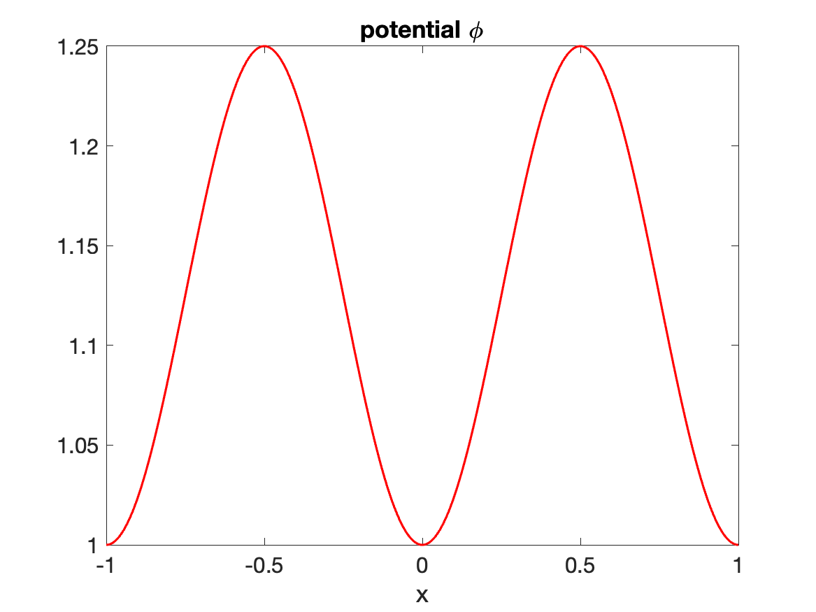
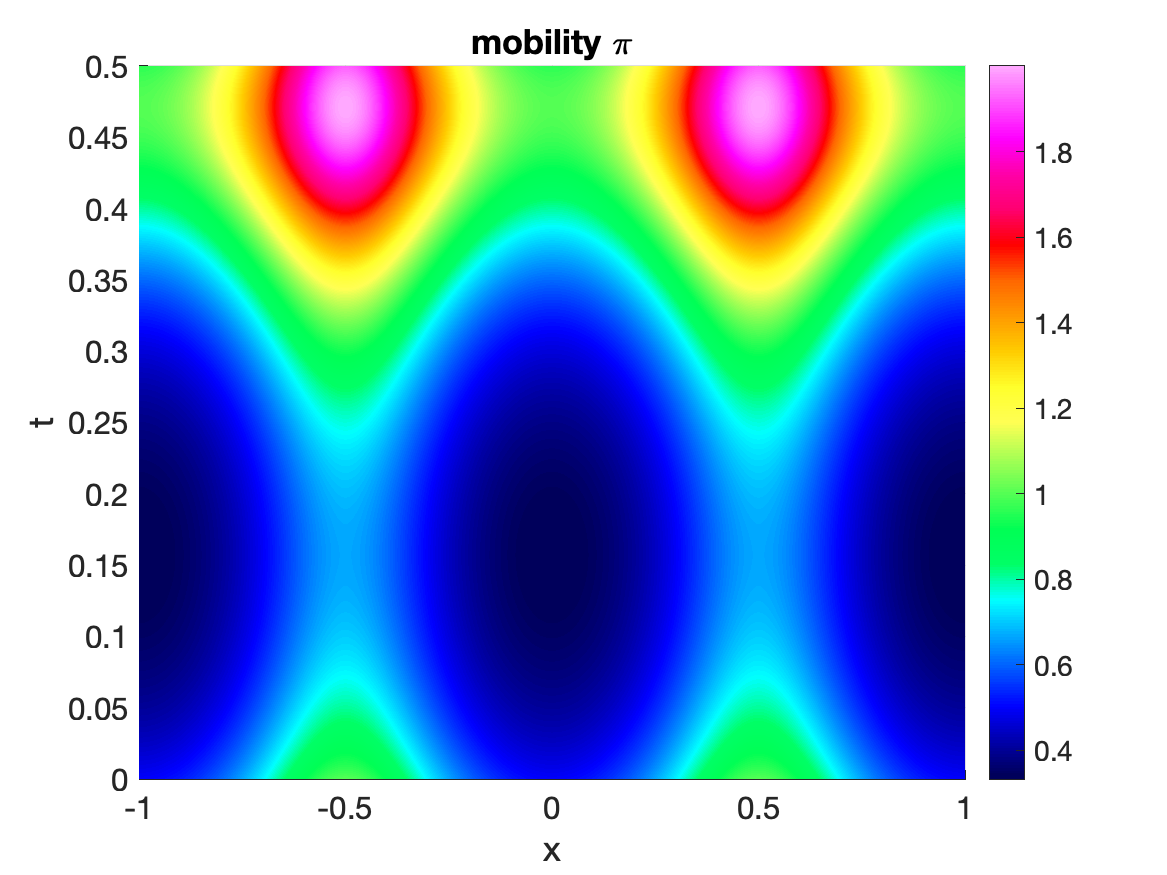
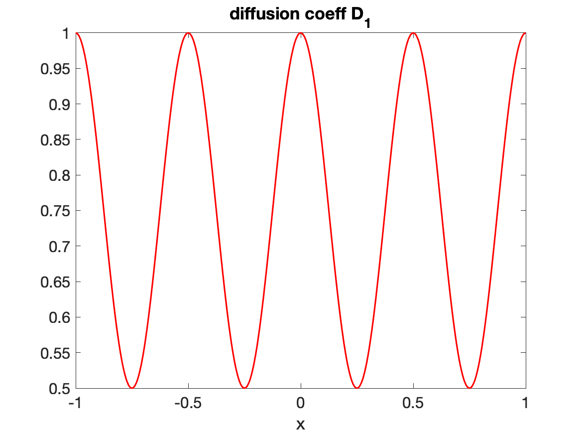
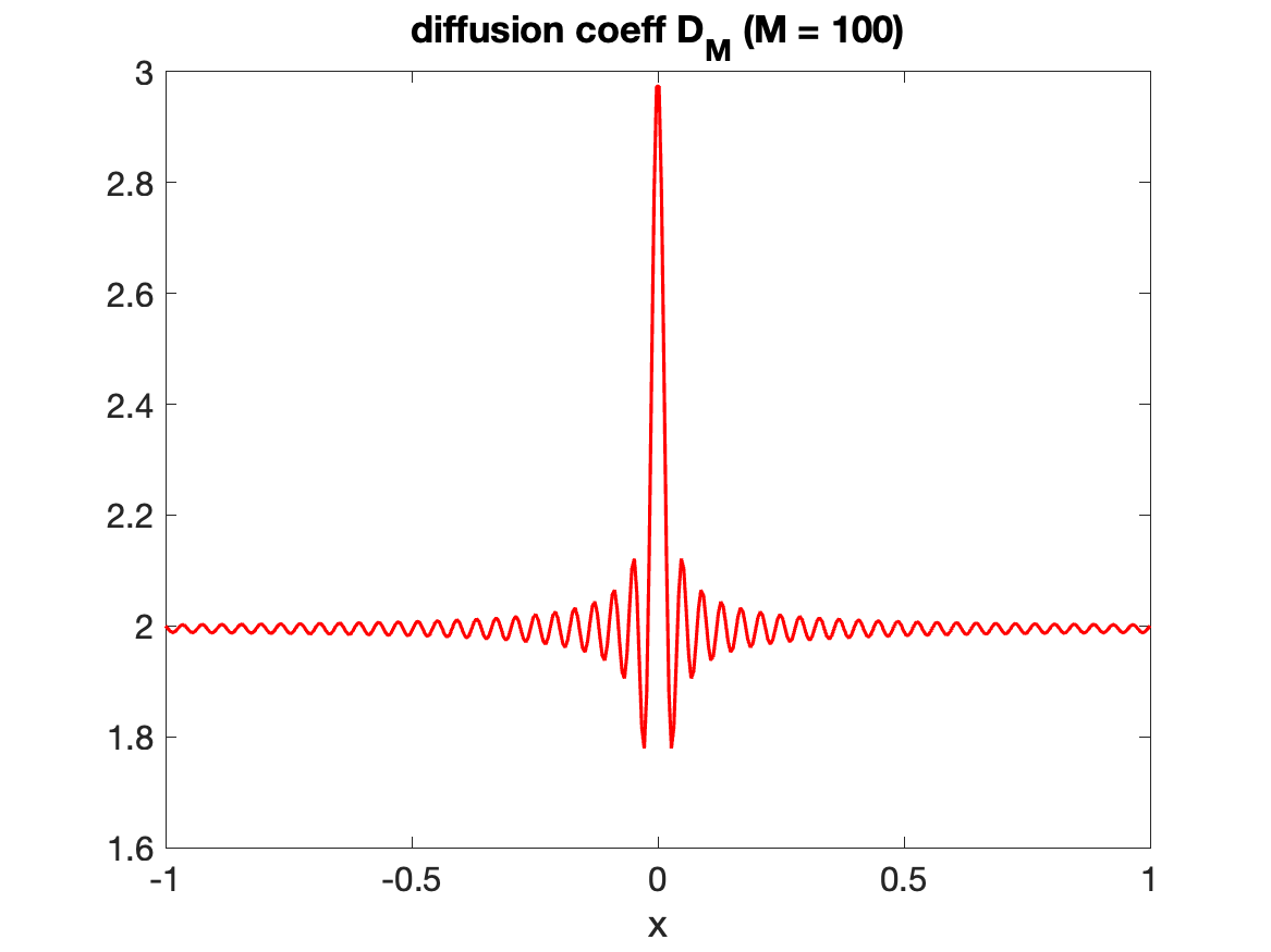
Figure 1. Periodic parameters in one dimension on $\Omega=[-1,\ 1]$. Top left: potential $\phi(x)$ (5.1) with $k_{p}=2$. Top right: mobility $\pi(x,\ t)$ (5.3), $t\in[0,\ 0.5]$. Bottom: inhomogeneous diffusion coefficient $D(x)$; left: single-mode $D_{1}(x)$ (5.4); right: multi-mode $D_{M}(x)$ (5.5) with $M=100$ modes of oscillation, and $A_{m}=0.01$.

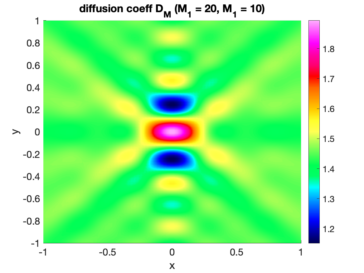
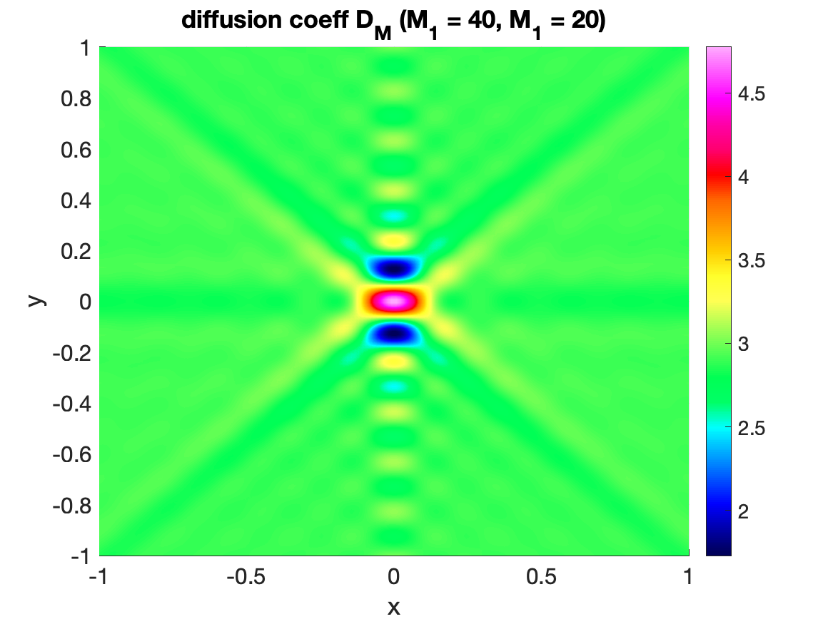
Figure 2. Multi-mode inhomogeneous diffusion coefficient $D_{M_{1},\ M_{2}}(x,\ y)$ (5.13), with $(M_{1},\ M_{2})$ modes of oscillation, and $A_{m_{1}m_{2}}=10^{-2}$ if $m_{1}<m_{2}$, and 0 otherwise. Left: $(M_{1},\ M_{2})=(20,\ 10)$; right: $(M_{1},\ M_{2})=(40,\ 20)$.

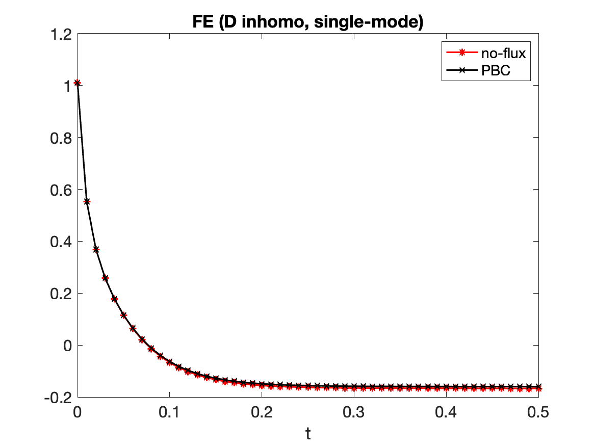
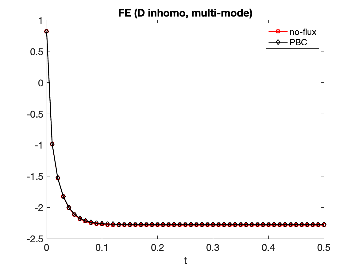
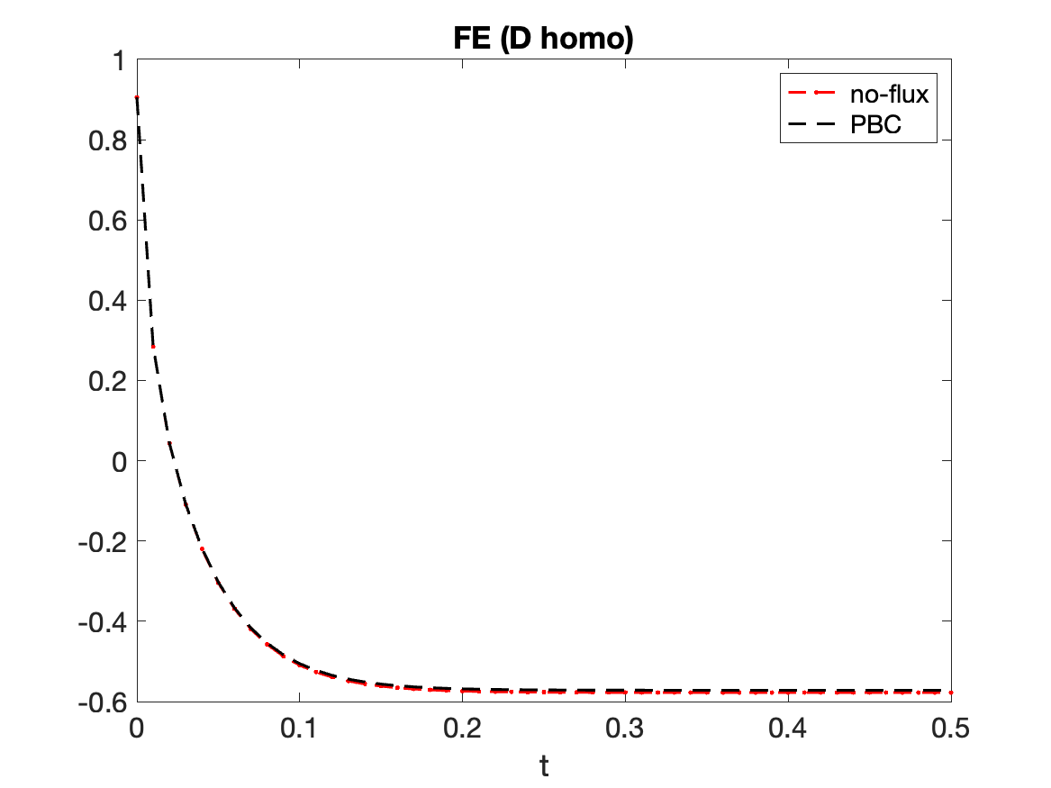
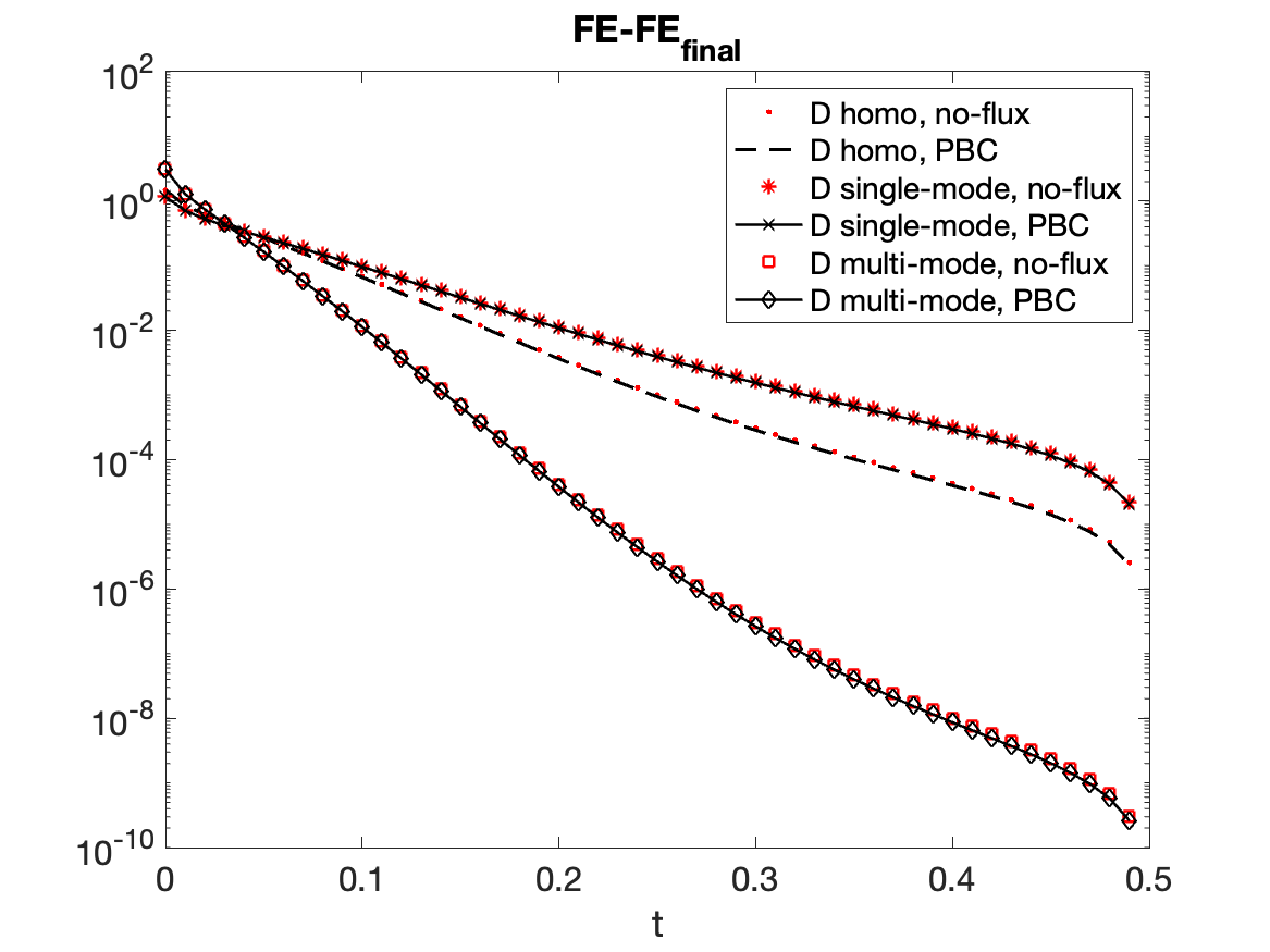
Figure 3. Exponential decay of free energy (FE), in one dimension, comparing no-flux (red) against periodic (black) boundary condition. Top: inhomogeneous $D(x)$; left: single-mode $D_{1}$ (5.4) (Figure 1, bottom left); right: multi-mode $D_{M}$ (5.5), with $M=N/2=100,\ A_{m}=0.01$ (Figure 1, bottom right). Bottom left: homogeneous $D=1$. Bottom right: direct comparison of the exponential decay rates. ($N_{\text{tot}}\approx 200\times 50.$)

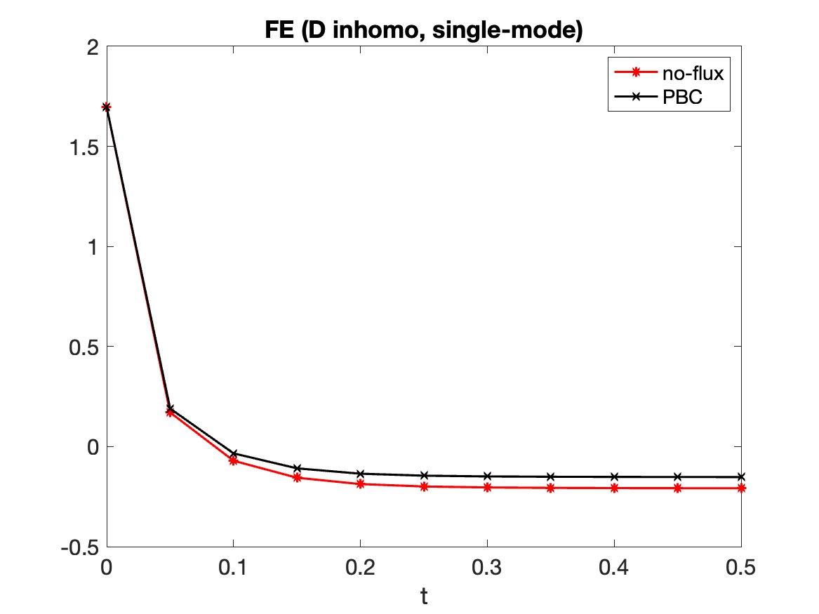
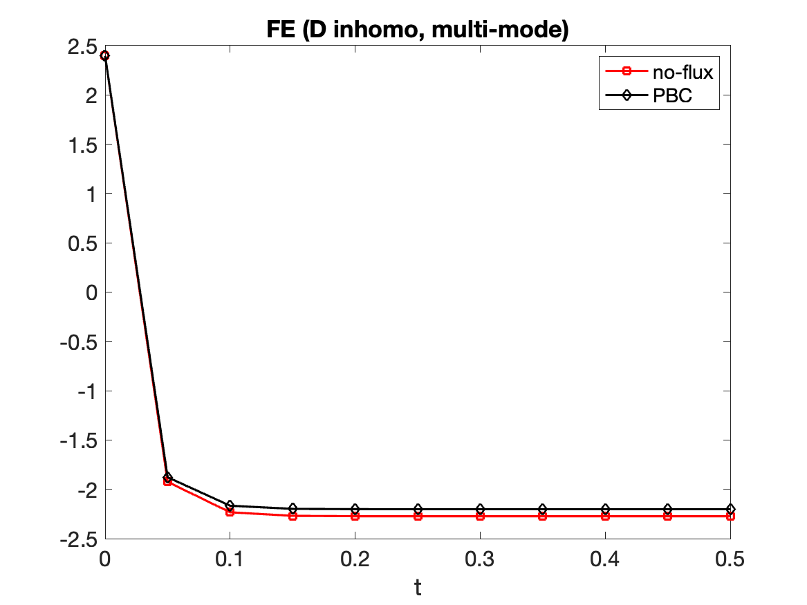
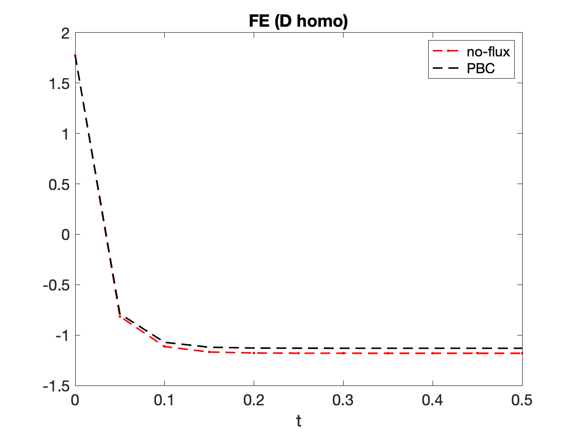
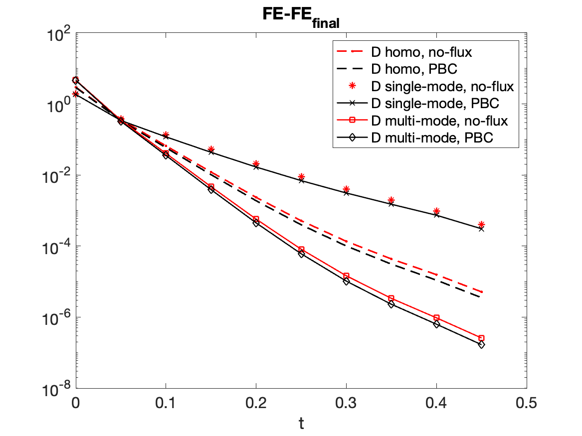
Figure 4. Exponential decay of free energy (FE), in two dimensions, comparing no-flux (red) against periodic (black) boundary condition. Top: inhomogeneous $D(\mathbf{x})$; left: single-mode $D_{1}$ (5.11); right: multi-mode $D_{M_{1},\ M_{2}}$ (5.13) with $(M_{1},\ M_{2})=(20,\ 10),\ A_{m_{1}m_{2}}=0.01$ if $m_{1}<m_{2}$, and 0 otherwise (Figure 2, left). Bottom left: homogeneous $D=1$. Bottom right: direct comparison of the exponential decay rates. ($N_{\text{tot}}\approx 40^{2}\times 10.$)

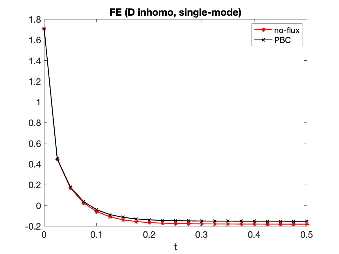
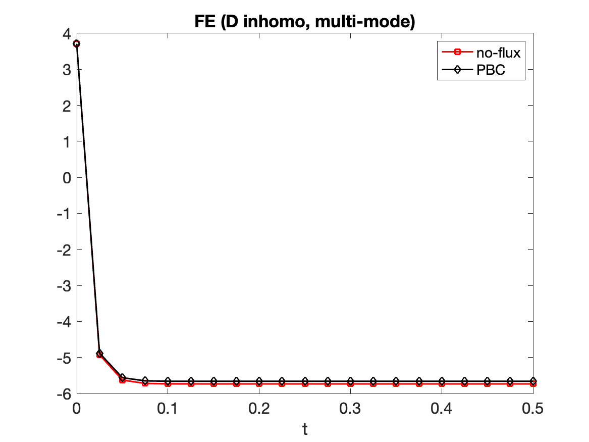
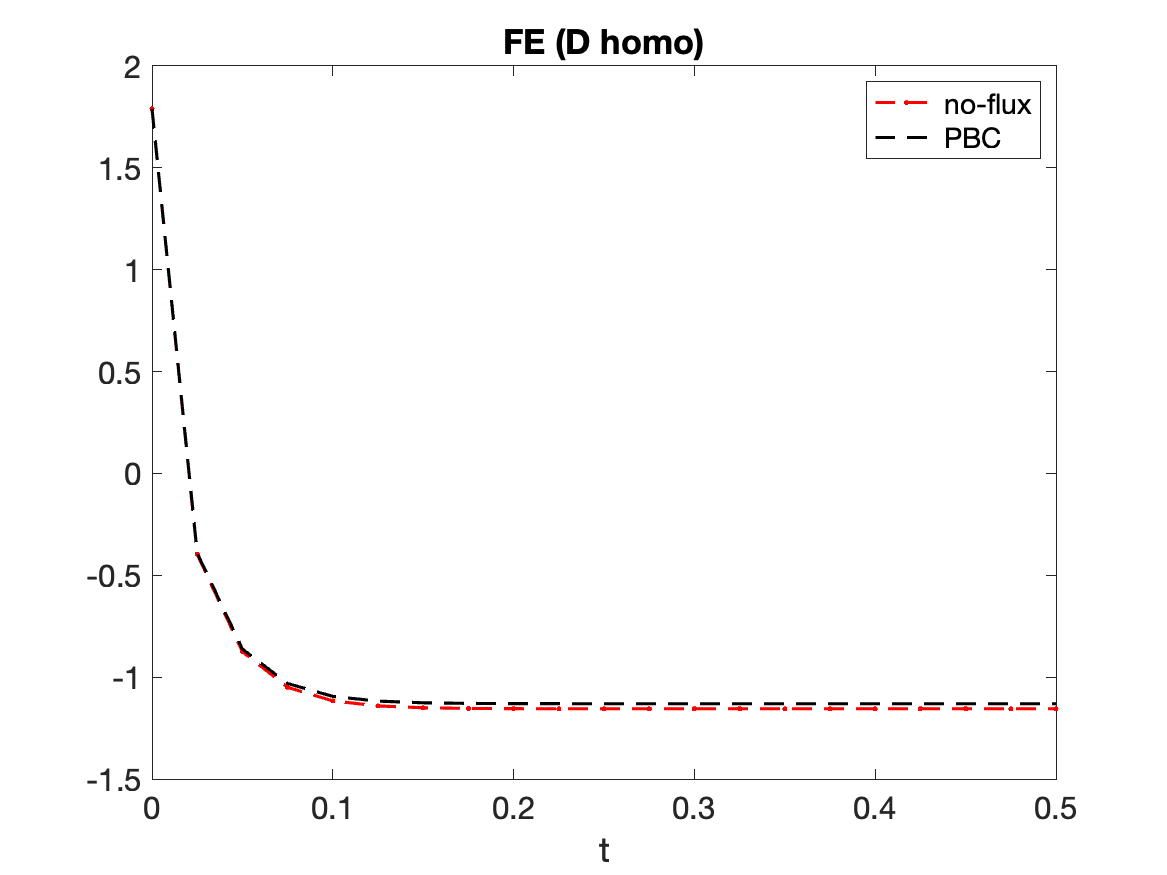
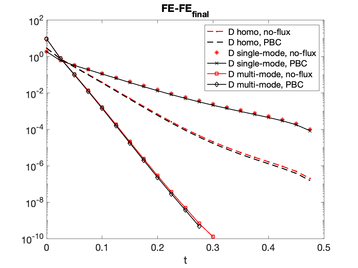
Figure 5. Exponential decay of free energy (FE), in two dimensions, comparing no-flux (red) against periodic (black) boundary condition. Top: inhomogeneous $D(\mathbf{x})$; left: single-mode $D_{1}$ (5.11); right: multi-mode $D_{M_{1},\ M_{2}}$ (5.13) with $(M_{1},\ M_{2})=(40,\ 20),\ A_{m_{1}m_{2}}=0.01$ if $m_{1}<m_{2}$, and 0 otherwise (Figure 2, right). Bottom left: homogeneous $D=1$. Bottom right: direct comparison of the exponential decay rates. ($N_{\text{tot}}\approx 80^{2}\times 20.$)

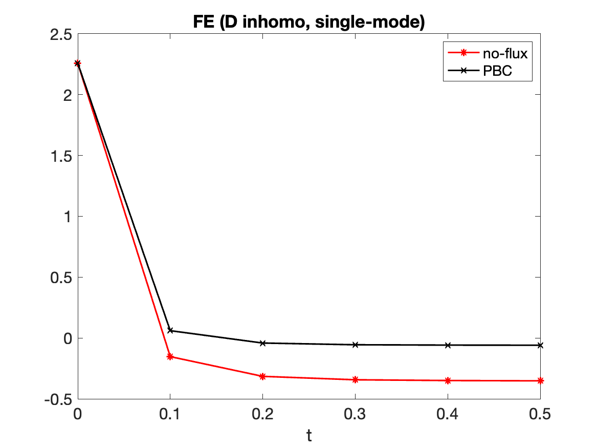
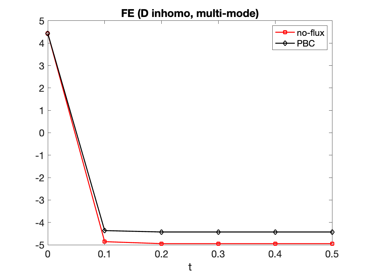
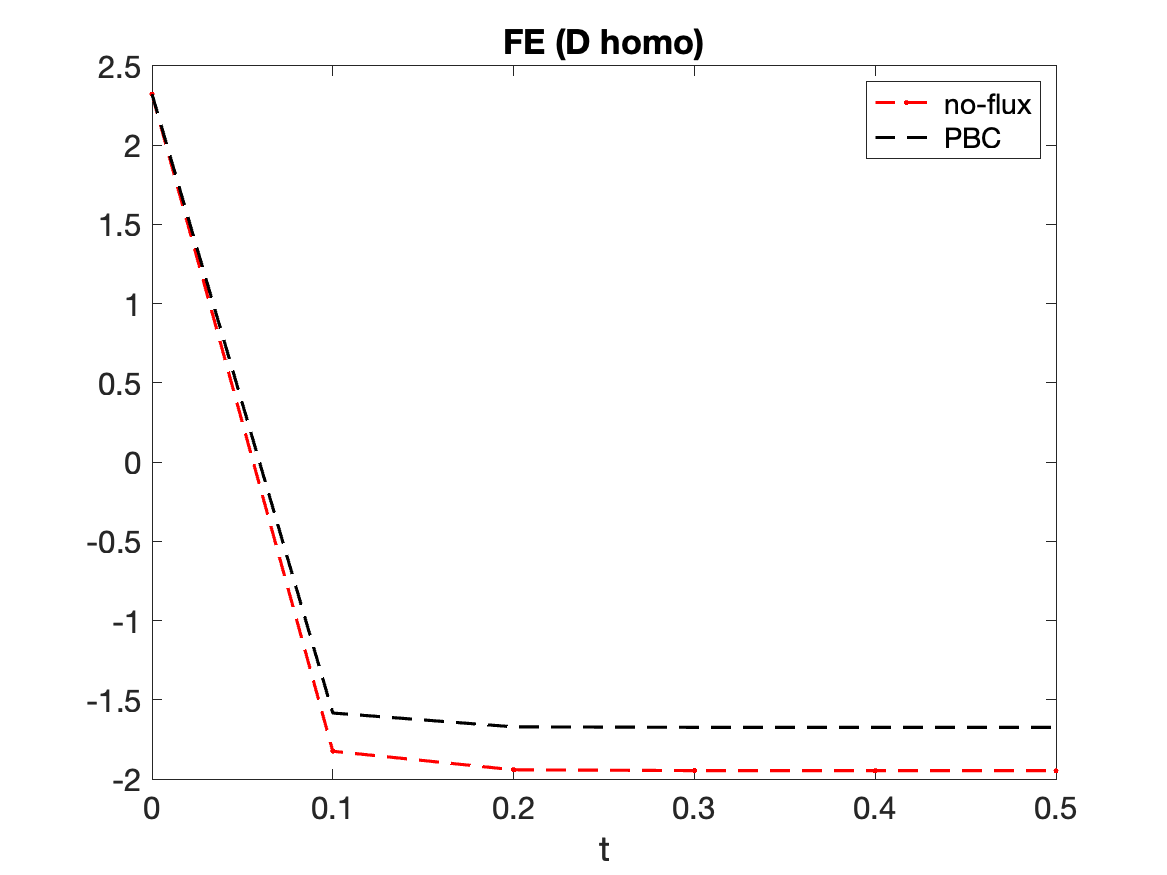
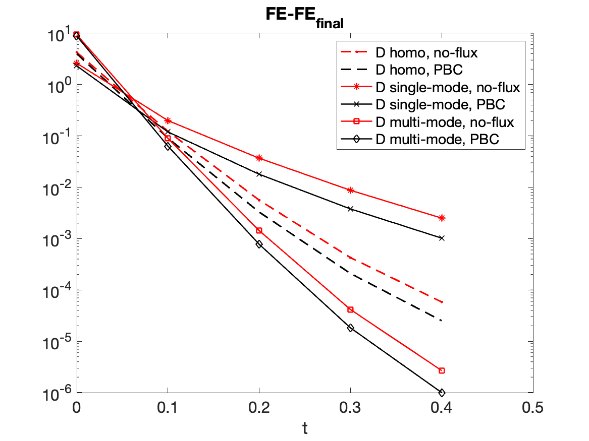
Figure 6. Exponential decay of free energy (FE), in three dimensions, comparing no-flux (red) against periodic (black) boundary condition. Top: inhomogeneous $D(\mathbf{x})$; left: single-mode (5.12); right: multi-mode (5.14) with $(M_{1},\ M_{2},\ M_{3})=(5,\ 3,\ 4),\ A_{m_{1}m_{2}m_{3}}=0.04$ if $m_{1}\geq m_{2}\geq m_{3}$, and 0 otherwise. Bottom left: homogeneous $D=1$. Bottom right: direct comparison of the exponential decay rates. ($N_{\text{tot}}\approx 10^{3}\times 5.$)

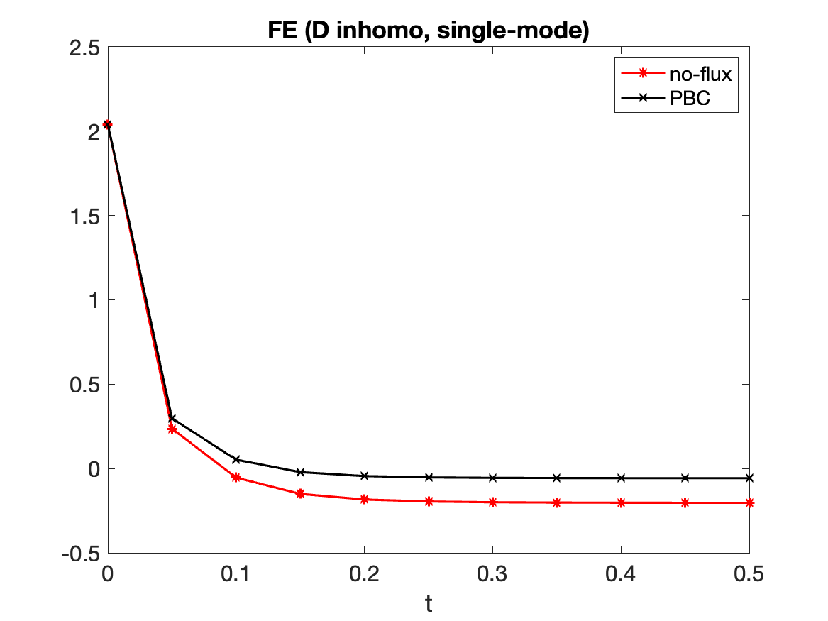
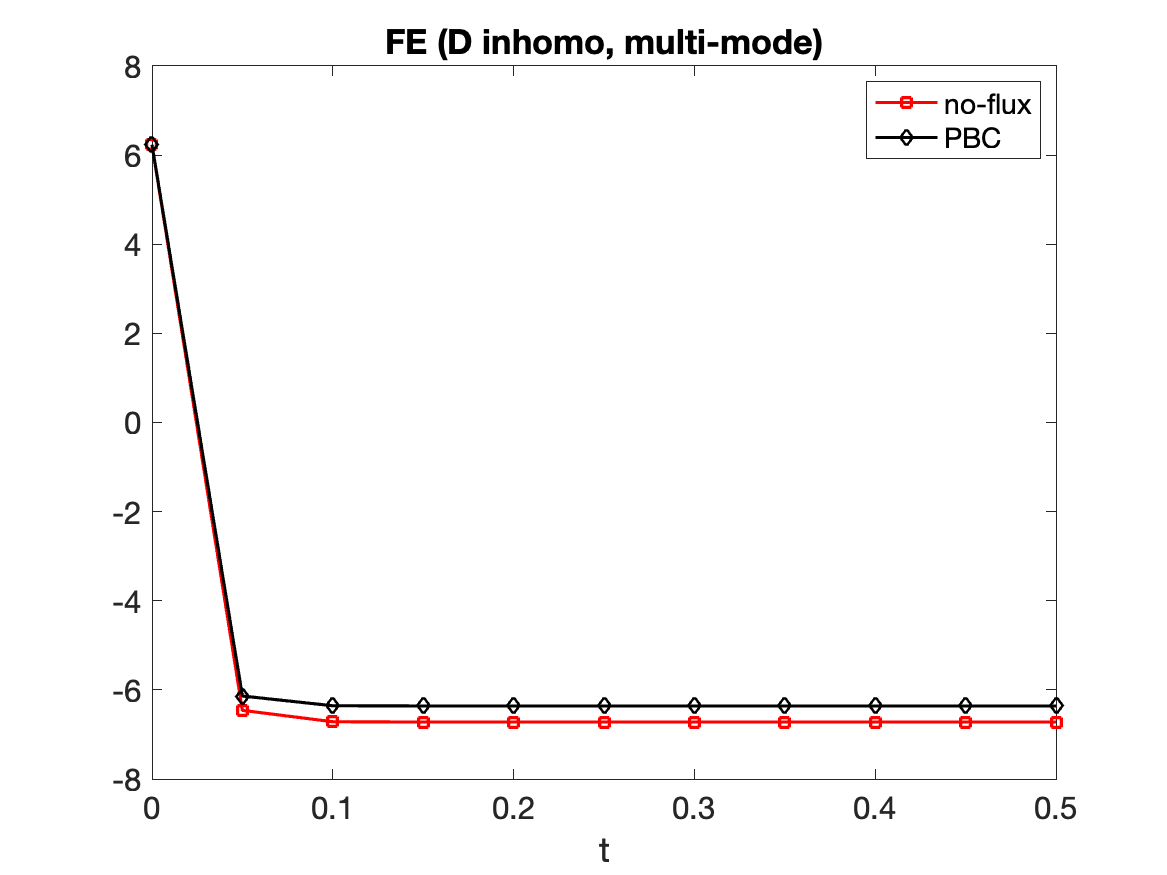
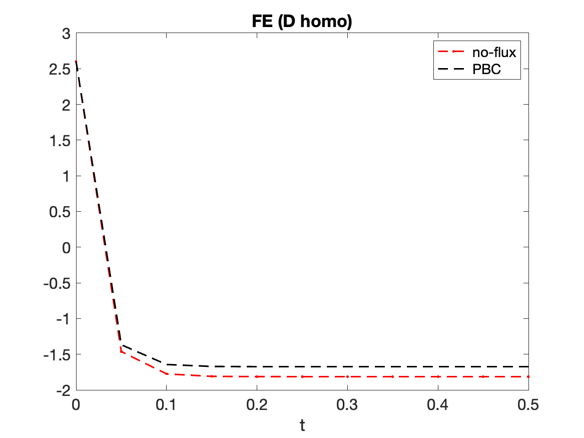
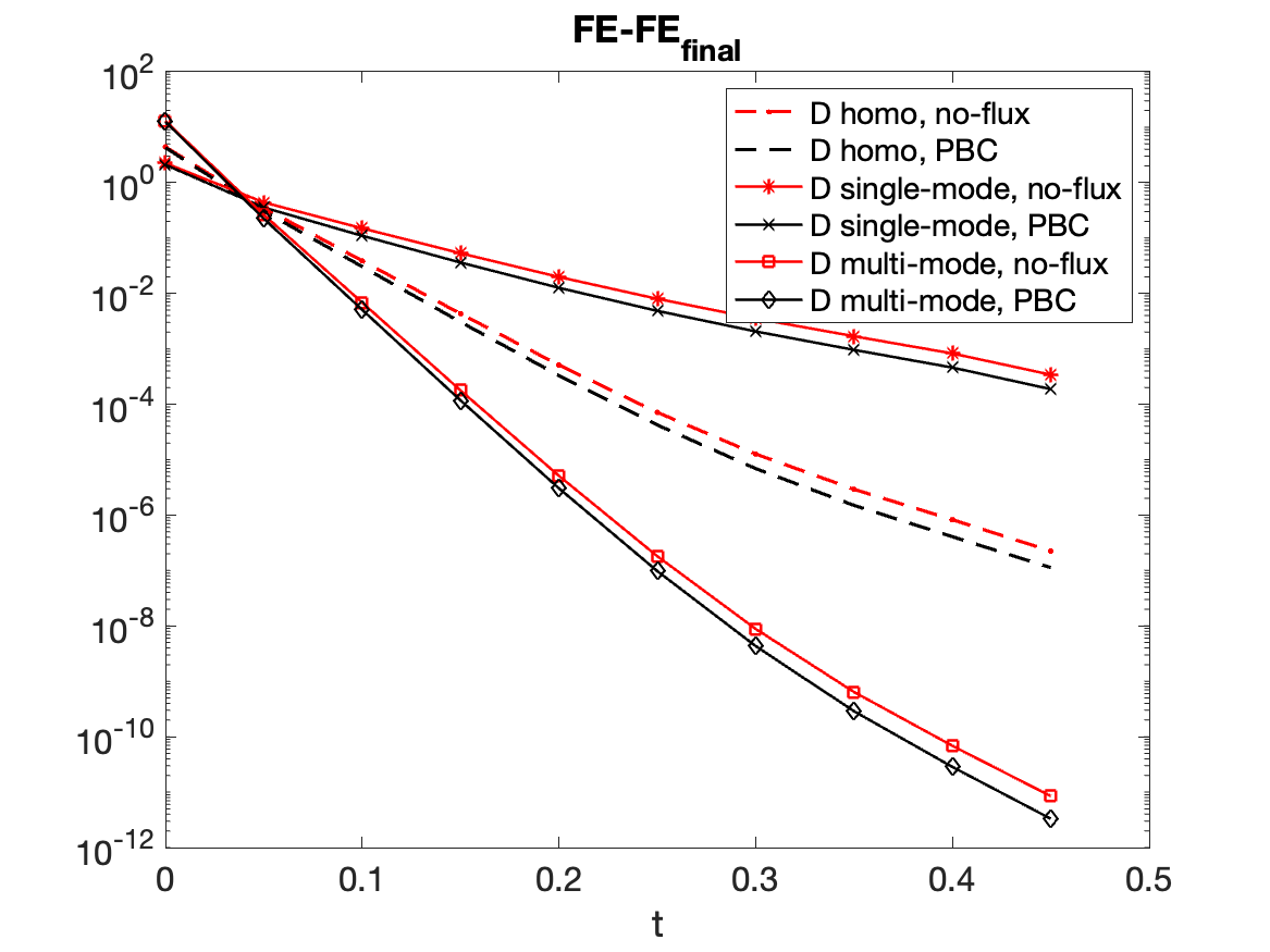
Figure 7. Exponential decay of free energy (FE), in three dimensions, comparing no-flux (red) against periodic (black) boundary condition. Top: inhomogeneous $D(\mathbf{x})$; left: single-mode (5.12); right: multi-mode (5.14) with $(M_{1},\ M_{2},\ M_{3})=(10,\ 8,\ 4),\ A_{m_{1}m_{2}m_{3}}=0.01$ if $m_{1}\geq m_{2}\geq m_{3}$, and 0 otherwise. Bottom left: homogeneous $D=1$. Bottom right: direct comparison of the exponential decay rates. ($N_{\text{tot}}\approx 20^{3}\times 10.$)

Appendix A The Cauchy problem for linear homogeneous Fokker-Planck equation

In this appendix, as noticed in Remark 2.10, we will reformulate the entropy dissipation method [34] for the Cauchy problem of the linear homogeneous Fokker-Planck equation in the framework of the general diffusion, in particular, the velocity field $\bm{u}$.

Here, we consider the following problem,

(A.1) $$\left\{\begin{aligned} \frac{\partial f}{\partial t}+\operatorname{div}\left(f\bm{u}\right)&=0,&\quad&x\in\mathbb{R}^{n},\quad t>0,\\ \bm{u}&=-\nabla\left(D\log f+\phi(x)\right),&\quad&x\in\mathbb{R}^{n},\quad t>0,\\ f(x,0)&=f_{0}(x),&\quad&x\in\mathbb{R}^{n},\end{aligned}\right.$$

where $D>0$ is a positive constant and $\phi=\phi(x)$ is a smooth function on $\mathbb{R}^{n}$. The free energy $F$ and the energy law (A.1) take the form,

(A.2) $$F[f]:=\int_{\mathbb{R}^{n}}\left(Df(\log f-1)+f\phi(x)\right)\,dx,$$

and

(A.3) $$\frac{dF}{dt}[f](t)=-\int_{\mathbb{R}^{n}}|\bm{u}|^{2}f\,dx:=-D_{\mathrm{dis}}[f](t).$$

Following the same argument from Section 2, as stated in Proposition 2.9 and Theorem 2.1, we can obtain the following assertion.

Proposition A.1.

Let $f$ be a solution of (A.1) and let $\bm{u}$ be defined in (A.1). Then,

(A.4) $$\frac{d^{2}F}{dt^{2}}[f](t)=2\int_{\mathbb{R}^{n}}((\nabla^{2}\phi(x))\bm{u}\cdot\bm{u})f\,dx+2\int_{\mathbb{R}^{n}}D|\nabla\bm{u}|^{2}f\,dx.$$

Proposition A.2.

Let $\phi=\phi(x)$ be a function on $\mathbb{R}^{n}$, and let $f_{0}=f_{0}(x)$ be a probability density function on $\mathbb{R}^{n}$, satisfying $F[f_{0}]<\infty$ and $D_{\mathrm{dis}}[f_{0}]<\infty$, where $F$ and $D_{\mathrm{dis}}[f_{0}]$ are defined by (A.2) and (A.3). Let $f$ be a solution of (A.1). Let $\bm{u}$ be defined as in (A.1). Assume further that there is a positive constant $\lambda>0$, such that $\nabla^{2}\phi\geq\lambda I$, where $I$ is the identity matrix. Then, the following is true,

(A.5) $$\int_{\mathbb{R}^{n}}|\bm{u}|^{2}f\,dx\leq e^{-2\lambda t}\int_{\mathbb{R}^{n}}|\nabla\left(D\log f_{0}+\phi(x)\right)|^{2}f_{0}\,dx.$$

In particular, we have that,

(A.6) $$\frac{dF}{dt}[f](t)=-\int_{\mathbb{R}^{n}}|\bm{u}|^{2}f\,dx\rightarrow 0,\qquad\text{as}\ t\rightarrow\infty.$$

Again as we note in Remark 2.10, from this proposition A.2, we can obtain the exponential decay of $\frac{dF}{dt}[f](t)=:-D_{\mathrm{dis}}[f](t)$, but not necessarily the long-time asymptotic behavior of the free energy $F[f](t)$ or the solution $f(t)$. The next theorem A.3 gives a stronger convergence result, namely, exponential convergence of $f$ to $f^{\mathrm{eq}}$ in the $L^{1}$ space as $t\rightarrow\infty$.

Theorem A.3.

Let $\phi=\phi(x)$ be a function on $\mathbb{R}^{n}$, and $f_{0}=f_{0}(x)$ be a probability density function on $\mathbb{R}^{n}$. Assume that $f$ is a solution of (A.1), $\bm{u}$ is defined as in (A.1), and there is a positive constant $\lambda>0$, such that, $\nabla^{2}\phi\geq\lambda I$, where $I$ is the identity matrix. Further, assume that $F[f_{0}]<\infty$ and $D_{\mathrm{dis}}[f_{0}]<\infty$, where $F$ and $D_{\mathrm{dis}}[f_{0}]$ are defined by (A.2) and (A.3). Then, any smooth solution of (A.1) converges exponentially fast to the equilibrium state, that is, there is a positive constant $\Cl{const:A.1}>0$ which depends only on $D$, $F[f^{\mathrm{eq}}]$ and $F[f_{0}]$ such that,

(A.7) $$\|f-f^{\mathrm{eq}}\|_{L^{1}(\mathbb{R}^{n})}\leq\Cr{const:A.1}e^{-\lambda t},\qquad t>0.$$

Key ideas to show Theorem A.3 are two inequalities. One is the Gross logarithmic Sobolev inequality [31]. The logarithmic Sobolev inequality and (A.6) deduce the convergence of $F[f](t)$ to $F[f^{\mathrm{eq}}]$ as $t\rightarrow\infty$. Using $\nabla^{2}\phi\geq\lambda I$ and Proposition A.1, we can show that the relative entropy convergences exponentially fast, $F[f](t)$ converges exponentially to $F[f^{\mathrm{eq}}]$, as $t\rightarrow\infty$. The other key inequality is the classical Csiszár-Kullback-Pinsker inequality [34] which connects $L^{1}$ convergence of $f$ to $f^{\mathrm{eq}}$ and the relative entropy convergence. Thus, we obtain the exponential convergence of $f$ in $L^{1}$ spaces.

Now, we show that $F[f](t)$ converges to $F[f^{\mathrm{eq}}]$ as $t\rightarrow\infty$. The following Gross logarithmic Sobolev inequality,

(A.8) $$\int_{\mathbb{R}^{n}}g^{2}\log\left(\frac{g^{2}}{\int_{\mathbb{R}^{n}}g^{2}\,d\mu}\right)\,d\mu\leq 2\int_{\mathbb{R}^{n}}|\nabla g|^{2}\,d\mu,$$

helps to show that the relative entropy $F[f](t)-F[f^{\mathrm{eq}}]\to 0$ as $t\rightarrow\infty$, where $d\mu=f^{\mathrm{eq}}\,dx$ and $g\in H^{1}(d\mu)$, (see [31]).

Lemma A.4.

Assume, that there is a positive constant $\lambda>0$ such that $\nabla^{2}\phi\geq\lambda I$, where $I$ is the identity matirx. Let $f$ be a solution of (A.1). Then,

(A.9) $$F[f](t)\rightarrow F[f^{\mathrm{eq}}],\qquad\text{as}\ t\rightarrow\infty.$$

Proof.

From (A.3), $F[f](t)$ is monotone decreasing, so we can give the estimate of $F[f](t)-F[f^{\mathrm{eq}}]$. By direct calculation of $F[f](t)-F[f^{\mathrm{eq}}]$ together with $D\log f^{\mathrm{eq}}+\phi=\Cr{const:1.1}$, (1.10), we obtain that,

$$F[f](t)-F[f^{\mathrm{eq}}]=\int_{\mathbb{R}^{n}}(Df\log f-Df+f\phi+Df^{\mathrm{eq}}-\Cr{const:1.1}f^{\mathrm{eq}})\,dx.$$

Using $\phi=\Cr{const:1.1}-D\log f^{\mathrm{eq}}$ and $\int_{\mathbb{R}^{n}}f\,dx=\int_{\mathbb{R}^{n}}f^{\mathrm{eq}}\,dx=1$, we have that,

(A.10) $$F[f](t)-F[f^{\mathrm{eq}}]=\int_{\mathbb{R}^{n}}D(f\log f-f\log f^{\mathrm{eq}})\,dx.$$

Recall that $\rho=f/f^{\mathrm{eq}}$ and,

$$F[f](t)-F[f^{\mathrm{eq}}]=D\int_{\mathbb{R}^{n}}\rho\log\rho f^{\mathrm{eq}}\,dx.$$

Since $s\log s$ is a convex function on $s>0$, we can apply the Jensen’s inequality [38] and (1.6) to have,

$$\int_{\mathbb{R}^{n}}\rho\log\rho f^{\mathrm{eq}}\,dx\geq\left(\int_{\mathbb{R}^{n}}\rho f^{\mathrm{eq}}\,dx\right)\log\left(\int_{\mathbb{R}^{n}}\rho f^{\mathrm{eq}}\,dx\right)\geq 0,$$

hence $f[f](t)-F[f^{\mathrm{eq}}]\geq 0$.

Put $g=\sqrt{\rho}$ to (A.8), where $\rho=f/f^{\mathrm{eq}}$. Since $\int_{\mathbb{R}^{n}}\rho\,d\mu=\int_{\mathbb{R}^{n}}f\,dx=1$, we have,

(A.11) $$\int_{\mathbb{R}^{n}}\rho\log\rho f^{\mathrm{eq}}\,dx\leq 2\int_{\mathbb{R}^{n}}|\nabla\sqrt{\rho}|^{2}f^{\mathrm{eq}}\,dx.$$

Using $\rho\log\rho f^{\mathrm{eq}}=f\log f-f\log f^{\mathrm{eq}}$, (A.10), and (A.11), we obtain that,

(A.12) $$F[f](t)-F[f^{\mathrm{eq}}]\leq 2D\int_{\mathbb{R}^{n}}|\nabla\sqrt{\rho}|^{2}f^{\mathrm{eq}}\,dx.$$

By direct calculation of $|\bm{u}|^{2}f$ and $|\nabla\sqrt{\rho}|^{2}f^{\mathrm{eq}}$, we obtain,

$$|\bm{u}|^{2}f=|\nabla(D\log\rho)|^{2}f=D^{2}\frac{|\nabla\rho|^{2}}{\rho^{2}}f,$$

and

$$|\nabla\sqrt{\rho}|^{2}f^{\mathrm{eq}}=\left|\frac{1}{2}\rho^{-\frac{1}{2}}\nabla\rho\right|^{2}f^{\mathrm{eq}}=\frac{1}{4}\frac{|\nabla\rho|^{2}}{\rho}f^{\mathrm{eq}}=\frac{1}{4}\frac{|\nabla\rho|^{2}}{\rho^{2}}f=\frac{1}{4D^{2}}|\bm{u}|^{2}f.$$

Hence, we have,

(A.13) $$2D\int_{\mathbb{R}^{n}}|\nabla\sqrt{\rho}|^{2}f^{\mathrm{eq}}\,dx=\frac{1}{2D}\int_{\mathbb{R}^{n}}|\bm{u}|^{2}f\,dx.$$

Combining (A.12), (A.13), and (A.6), we have $F[f](t)\rightarrow F[f^{\mathrm{eq}}]$ as $t\rightarrow\infty$. ∎

Note that, in the proof of Lemma A.4, we obtain due to (A.10) that,

(A.14) $$F[f](t)-F[f^{\mathrm{eq}}]=\int_{\mathbb{R}^{n}}D(f\log f-f\log f^{\mathrm{eq}})\,dx.$$

We next derive exponential decay of the relative entropy $F[f](t)-F[f^{\mathrm{eq}}]$.

Lemma A.5.

Assume, that there is a positive constant $\lambda>0$ such that $\nabla^{2}\phi\geq\lambda I$, where $I$ is the identity matirx and $F[f_{0}]<0$. Let $f$ be a solution of (A.1). Then, we obtain for $t>0$,

(A.15) $$(F[f](t)-F[f^{\mathrm{eq}}])\leq e^{-2\lambda t}(F[f_{0}]-F[f^{\mathrm{eq}}]).$$

Proof.

First, from (A.3) and (A.4), due to the convexity assumption $\nabla^{2}\phi(x)\geq\lambda$, we have that,

$$\frac{d^{2}F}{dt^{2}}[f](t)\geq 2\lambda\int_{\mathbb{R}^{n}}|\bm{u}|^{2}f\,dx=-2\lambda\frac{dF}{dt}[f](t).$$

Integrating on $[t,s]$, we obtain,

$$\frac{dF}{dt}[f](s)-\frac{dF}{dt}[f](t)\geq 2\lambda(F[f](t)-F[f](s)).$$

Taking $s\rightarrow\infty$ together with (A.6), (A.9), and $\frac{d}{dt}F[f^{\mathrm{eq}}]=0$, we arrive at,

(A.16) $$\frac{d}{dt}(F[f](t)-F[f^{\mathrm{eq}}])\leq-2\lambda(F[f](t)-F[f^{\mathrm{eq}}]).$$

Using the Gronwall’s inequality in (A.16) and $F[f_{0}]<\infty$, we obtain the result (A.15). ∎

Next, we state the classical Csiszár-Kullback-Pinsker inequality, in order to combine $L^{1}$ norm and the relative entropy $F[f](t)-F[f^{\mathrm{eq}}]$.

Proposition A.6 (Classical Csiszár-Kullback-Pinsker inequality [34]).

Let $\Omega\subset\mathbb{R}^{n}$ be a domain, let $f,g\in L^{1}(\Omega)$ satisfy $f\geq 0$, $g>0$, and $\int_{\Omega}f\,dx=\int_{\Omega}g\,dx=1$. Then,

(A.17) $$\|f-g\|_{L^{1}(\Omega)}^{2}\leq 2\int_{\Omega}(f\log f-f\log g)\,dx.$$

Using the classical Csiszár-Kullback-Pinsker inequality, we show Theorem A.3.

Proof of Theorem A.3.

Combining (A.14) and (A.15), we have that,

(A.18) $$\int_{\mathbb{R}^{n}}(f\log f-f\log f^{\mathrm{eq}})\,dx=\frac{1}{D}(F[f](t)-F[f^{\mathrm{eq}}])\leq\frac{1}{D}(F[f_{0}]-F[f^{\mathrm{eq}}])e^{-2\lambda t}.$$

Combining (A.18) and the classical Csiszár-Kullback-Pinsker inequality (A.17), we have,

$$\|f-f^{\mathrm{eq}}\|_{L^{1}(\mathbb{R}^{n})}^{2}\leq\frac{2}{D}(F[f_{0}]-F[f^{\mathrm{eq}}])e^{-2\lambda t},$$

Hence, we obtain (A.7) by selecting $\Cr{const:A.1}=\sqrt{\frac{2}{D}(F[f_{0}]-F[f^{\mathrm{eq}}])}$. ∎

Remark A.7.

The strict convexity for $\phi$ is essential for the entropy dissipation method. On the other hand, if $\phi$ is not strictly convex, we can proceed to study the long-time asymptotic behavior in the weighted $L^{2}$ space $L^{2}(\Omega,e^{\phi/D}\,dx)$ [2, 22]. Using the result of the asymptotics in the weighted $L^{2}$ space, we may show Lemma A.4 and Lemma A.5 without using the Gross logarithmic Sobolev inequality. Furthermore, it is known that the logarithmic Sobolev inequality can be deduced from the differential inequality (A.16) of the relative entropy [34], Thus, there is a close relationship among the long-time asymptotics in the weighted $L^{2}$ space, the logarithmic Sobolev inequality, the differential inequality (A.16) and the exponential decay for the relative entropy (A.15).

References

[1]
Robert A. Adams and John J. F. Fournier.
Sobolev spaces, volume 140 of Pure and Applied Mathematics
(Amsterdam).
Elsevier/Academic Press, Amsterdam, second edition, 2003.
[2]
Anton Arnold, Peter Markowich, Giuseppe Toscani, and Andreas Unterreiter.
On convex Sobolev inequalities and the rate of convergence to
equilibrium for Fokker-Planck type equations.
Comm. Partial Differential Equations, 26(1-2):43–100, 2001.
[3]
Ralph Baierlein.
Thermal Physics.
Cambridge University Press, 1999.
[4]
Patrick Bardsley, Katayun Barmak, Eva Eggeling, Yekaterina Epshteyn, David
Kinderlehrer, and Shlomo Ta’asan.
Towards a gradient flow for microstructure.
Atti Accad. Naz. Lincei Rend. Lincei Mat. Appl.,
28(4):777–805, 2017.
[5]
K. Barmak, E. Eggeling, M. Emelianenko, Y. Epshteyn, D. Kinderlehrer, R. Sharp,
and S. Ta’asan.
Critical events, entropy, and the grain boundary character
distribution.
Phys. Rev. B, 83:134117, Apr 2011.
[6]
K. Barmak, E. Eggeling, M. Emelianenko, Y. Epshteyn, D. Kinderlehrer, and
S. Ta’asan.
Geometric growth and character development in large metastable
networks.
Rend. Mat. Appl. (7), 29(1):65–81, 2009.
[7]
K. Barmak, E. Eggeling, D. Kinderlehrer, R. Sharp, S. Ta’asan, A.D. Rollett,
and K.R. Coffey.
Grain growth and the puzzle of its stagnation in thin films: The
curious tale of a tail and an ear.
Progress in Materials Science, 58(7):987–1055, 2013.
[8]
Katayun Barmak, Anastasia Dunca, Yekaterina Epshteyn, Chun Liu, and Masashi
Mizuno.
Grain growth and the effect of different time scales.
2022.
Springer AWM series volume ”Research in the Mathematics of Materials
Science”, In Press, arXiv:2105.07255.
[9]
Katayun Barmak, Eva Eggeling, Maria Emelianenko, Yekaterina Epshteyn, David
Kinderlehrer, Richard Sharp, and Shlomo Ta’asan.
An entropy based theory of the grain boundary character distribution.
Discrete Contin. Dyn. Syst., 30(2):427–454, 2011.
[10]
Giovanni Bellettini.
Lecture notes on mean curvature flow, barriers and singular
perturbations, volume 12 of Appunti. Scuola Normale Superiore di Pisa
(Nuova Serie) [Lecture Notes. Scuola Normale Superiore di Pisa (New
Series)].
Edizioni della Normale, Pisa, 2013.
[11]
R. Stephen Berry, Stuart Alan Rice, and John Ross.
Physical chemistry.
Topics in physical chemistry series. Oxford University Press, 2nd ed.
edition, 2000.
[12]
Aditi Bhattacharya, Yu-Feng Shen, Christopher M. Hefferan, Shiu Fai Li,
Jonathan Lind, Robert M. Suter, Carl E. Krill, and Gregory S. Rohrer.
Grain boundary velocity and curvature are not correlated in ni
polycrystals.
Science, 374(6564):189–193, 2021.
[13]
Kenneth A. Brakke.
The motion of a surface by its mean curvature, volume 20 of
Mathematical Notes.
Princeton University Press, Princeton, N.J., 1978.
[14]
Lia Bronsard and Fernando Reitich.
On three-phase boundary motion and the singular limit of a
vector-valued Ginzburg-Landau equation.
Arch. Rational Mech. Anal., 124(4):355–379, 1993.
[15]
José A. Cañizo, José A. Carrillo, Philippe Laurençot, and
Jesús Rosado.
The Fokker-Planck equation for bosons in 2D: well-posedness and
asymptotic behavior.
Nonlinear Anal., 137:291–305, 2016.
[16]
J. A. Carrillo and G. Toscani.
Exponential convergence toward equilibrium for homogeneous
Fokker-Planck-type equations.
Math. Methods Appl. Sci., 21(13):1269–1286, 1998.
[17]
José A. Carrillo, María D. M. González, Maria P. Gualdani, and
Maria E. Schonbek.
Classical solutions for a nonlinear Fokker-Planck equation
arising in computational neuroscience.
Comm. Partial Differential Equations, 38(3):385–409, 2013.
[18]
Yun Gang Chen, Yoshikazu Giga, and Shun’ichi Goto.
Uniqueness and existence of viscosity solutions of generalized mean
curvature flow equations.
J. Differential Geom., 33(3):749–786, 1991.
[19]
Pierre Degond, Maxime Herda, and Sepideh Mirrahimi.
A Fokker-Planck approach to the study of robustness in gene
expression.
Math. Biosci. Eng., 17(6):6459–6486, 2020.
[20]
Weinan E, Tiejun Li, and Eric Vanden-Eijnden.
Applied stochastic analysis, volume 199 of Graduate
Studies in Mathematics.
American Mathematical Society, Providence, RI, 2019.
[21]
Klaus Ecker.
Regularity theory for mean curvature flow.
Progress in Nonlinear Differential Equations and their Applications,
57. Birkhäuser Boston, Inc., Boston, MA, 2004.
[22]
Y. Epshteyn, C. Liu, and M. Mizuno.
A stochastic model of grain boundary dynamics: A Fokker-Planck
perspective, 2021.
submitted, arXiv:2106.14249.
[23]
Yekaterina Epshteyn, Chang Liu, Chun Liu, and Masashi Mizuno.
Local well-posedness of a nonlinear Fokker-Planck model, 2022,
submitted, arXiv:2201.09117.
[24]
Yekaterina Epshteyn, Chun Liu, and Masashi Mizuno.
Large time asymptotic behavior of grain boundaries motion with
dynamic lattice misorientations and with triple junctions drag.
Commun. Math. Sci., 19(5):1403–1428, 2021.
[25]
Yekaterina Epshteyn, Chun Liu, and Masashi Mizuno.
Motion of Grain Boundaries with Dynamic Lattice
Misorientations and with Triple Junctions Drag.
SIAM J. Math. Anal., 53(3):3072–3097, 2021.
[26]
J. L. Ericksen.
Introduction to the thermodynamics of solids, volume 131 of
Applied Mathematical Sciences.
Springer-Verlag, New York, revised edition, 1998.
[27]
L. C. Evans and J. Spruck.
Motion of level sets by mean curvature. I.
J. Differential Geom., 33(3):635–681, 1991.
[28]
Lawrence C. Evans.
Partial differential equations, volume 19 of Graduate
Studies in Mathematics.
American Mathematical Society, Providence, RI, second edition, 2010.
[29]
C. W. Gardiner.
Handbook of stochastic methods for physics, chemistry and the
natural sciences, volume 13 of Springer Series in Synergetics.
Springer-Verlag, Berlin, third edition, 2004.
[30]
Mi-Ho Giga, Arkadz Kirshtein, and Chun Liu.
Variational modeling and complex fluids.
In Handbook of mathematical analysis in mechanics of viscous
fluids, pages 73–113. Springer, Cham, 2018.
[31]
Leonard Gross.
Logarithmic Sobolev inequalities.
Amer. J. Math., 97(4):1061–1083, 1975.
[32]
Conyers Herring.
Surface tension as a motivation for sintering.
In Fundamental Contributions to the Continuum Theory of Evolving
Phase Interfaces in Solids, pages 33–69. Springer, 1999.
[33]
Jingwei Hu, Jian-Guo Liu, Yantong Xie, and Zhennan Zhou.
A structure preserving numerical scheme for Fokker-Planck
equations of neuron networks: numerical analysis and exploration.
J. Comput. Phys., 433:Paper No. 110195, 23, 2021.
[34]
Ansgar Jüngel.
Entropy methods for diffusive partial differential equations.
SpringerBriefs in Mathematics. Springer, [Cham], 2016.
[35]
Lami Kim and Yoshihiro Tonegawa.
On the mean curvature flow of grain boundaries.
Ann. Inst. Fourier (Grenoble), 67(1):43–142, 2017.
[36]
D Kinderlehrer and C Liu.
Evolution of grain boundaries.
Mathematical Models and Methods in Applied Sciences,
11(4):713–729, Jun 2001.
[37]
O. A. Ladyženskaja, V. A. Solonnikov, and N. N. Ural’ceva.
Linear and quasilinear equations of parabolic type.
Translated from the Russian by S. Smith. Translations of Mathematical
Monographs, Vol. 23. American Mathematical Society, Providence, R.I., 1967.
[38]
Elliott H. Lieb and Michael Loss.
Analysis, volume 14 of Graduate Studies in Mathematics.
American Mathematical Society, Providence, RI, second edition, 2001.
[39]
Gary M. Lieberman.
Second order parabolic differential equations.
World Scientific Publishing Co. Inc., River Edge, NJ, 1996.
[40]
Annibale Magni, Carlo Mantegazza, and Matteo Novaga.
Motion by curvature of planar networks, II.
Ann. Sc. Norm. Super. Pisa Cl. Sci. (5), 15:117–144, 2016.
[41]
Carlo Mantegazza, Matteo Novaga, and Alessandra Pluda.
Lectures on curvature flow of networks.
In Contemporary research in elliptic PDEs and related topics,
volume 33 of Springer INdAM Ser., pages 369–417. Springer, Cham, 2019.
[42]
Carlo Mantegazza, Matteo Novaga, and Vincenzo Maria Tortorelli.
Motion by curvature of planar networks.
Ann. Sc. Norm. Super. Pisa Cl. Sci. (5), 3(2):235–324, 2004.
[43]
P. A. Markowich and C. Villani.
On the trend to equilibrium for the Fokker-Planck equation: an
interplay between physics and functional analysis.
In VI Workshop on Partial Differential Equations, Part II (Rio
de Janeiro, 1999), volume 19, pages 1–29. Sociedade Brasileira de
Matemática, Rio de Janeiro, 2000.
[44]
Donald Allan McQuarrie.
Statistical mechanics.
Harper’s chemistry series. Harper & Row, 1976.
[45]
W. W. Mullins.
Two-dimensional motion of idealized grain boundaries.
Journal of Applied Physics, 27(8):900–904, 1956.
[46]
W. W. Mullins.
Theory of thermal grooving.
Journal of Applied Physics, 28(3):333–339, 1957.
[47]
Matthew Patrick, Gregory Rohrer, Ooraphan Chirayutthanasak, Sutatch Ratanaphan,
Eric Homer, Gus Hart, Yekaterina Epshteyn, and Katayun Barmak.
Relative grain boundary energies from triple junction geometry:
Limitations to assuming the Herring condition in nanocrystalline thin
films.
in final preparation, 2022.
[48]
Grigorios A. Pavliotis.
Stochastic processes and applications, volume 60 of Texts
in Applied Mathematics.
Springer, New York, 2014.
Diffusion processes, the Fokker-Planck and Langevin equations.
[49]
Murray H. Protter and Hans F. Weinberger.
Maximum principles in differential equations.
Springer-Verlag, New York, 1984.
Corrected reprint of the 1967 original.
[50]
H. Risken.
The Fokker-Planck equation, volume 18 of Springer
Series in Synergetics.
Springer-Verlag, Berlin, second edition, 1989.
Methods of solution and applications.
[51]
Silvio R. A. Salinas.
Introduction to statistical physics.
Graduate Texts in Contemporary Physics. Springer-Verlag, New York,
2001.
Translated from the Portuguese.
[52]
Gabriele Sicuro, Peter Rapčan, and Constantino
Tsallis.