SoteriaFL: A Unified Framework for Private Federated Learning with Communication Compression

Abstract

To enable large-scale machine learning in bandwidth-hungry environments such as wireless networks, significant progress has been made recently in designing communication-efficient federated learning algorithms with the aid of communication compression. On the other end, privacy-preserving, especially at the client level, is another important desideratum that has not been addressed simultaneously in the presence of advanced communication compression techniques yet. In this paper, we propose a unified framework that enhances the communication efficiency of private federated learning with communication compression. Exploiting both general compression operators and local differential privacy, we first examine a simple algorithm that applies compression directly to differentially-private stochastic gradient descent, and identify its limitations. We then propose a unified framework SoteriaFL for private federated learning, which accommodates a general family of local gradient estimators including popular stochastic variance-reduced gradient methods and the state-of-the-art shifted compression scheme. We provide a comprehensive characterization of its performance trade-offs in terms of privacy, utility, and communication complexity, where SoteriaFL is shown to achieve better communication complexity without sacrificing privacy nor utility than other private federated learning algorithms without communication compression.

Keywords: federated learning, local differential privacy, communication compression, unified framework

1 Introduction

With the proliferation of mobile and edge devices, federated learning (FL) [42, 55] has recently emerged as a disruptive paradigm for training large-scale machine learning models over a vast amount of geographically distributed and heterogeneous devices. For instance, Google uses FL in the Gboard mobile keyboard for next word predictions [29]. FL is often modeled as a distributed optimization problem [41, 42, 55, 35, 72], aiming to solve

$$\min_{{\bm{x}}\in\mathbb{R}^{d}}\left\{f({\bm{x}};D):=\frac{1}{n}\sum_{i=1}^{n}f({\bm{x}};D_{i})\right\},~{}~{}\text{where~{}}f({\bm{x}};D_{i}):=\frac{1}{m}\sum_{j=1}^{m}f({\bm{x}};d_{i,j}).$$ (1)

Here, $D$ denotes the entire dataset distributed across all $n$ clients, where each client $i$ has a local dataset $D_{i}=\{d_{i,j}\}_{j=1}^{m}$ of equal size $m$, ${\bm{x}}\in\mathbb{R}^{d}$ denotes the model parameters, $f({\bm{x}};D)$, $f({\bm{x}};D_{i})$, and $f({\bm{x}};d_{i,j})$ denote the nonconvex loss function of the current model ${\bm{x}}$ on the entire dataset $D$, the local dataset $D_{i}$, and a single data sample $d_{i,j}$, respectively. For simplicity, we use $f({\bm{x}})$, $f_{i}({\bm{x}})$ and $f_{i,j}({\bm{x}})$ to denote $f({\bm{x}};D)$, $f({\bm{x}};D_{i})$ and $f({\bm{x}};d_{i,j})$, respectively.

1.1 Motivation: privacy-utility-communication trade-offs

To unleash the full potential of FL, it is extremely important that the algorithm designed to solve (1) needs to meet several competing desiderata.

Communication efficiency.

Communication between the server and clients is well recognized as the main bottleneck for optimizing the latency of FL systems, especially when the clients—such as mobile devices—have limited bandwidth, the number of clients is large, and/or the machine learning model has a lot of parameters—for example, the language model GPT-3 [7] has billions of parameters and therefore cumbersome to share directly.

Therefore, it is very important to design FL algorithms to reduce the overall communication cost, which takes into account both the number of communication rounds and the cost per communication round for reaching a desired accuracy. With these two quantities in mind, there are two principal approaches for communication-efficient FL: 1) local methods, where in each communication round, clients run multiple local update steps before communicating with the server, in the hope of reducing the number of communication rounds, e.g., [55, 48, 39, 27, 38, 71, 60, 9, 47, 46, 2, 78, 58, 57]; 2) compression methods, where clients send compressed communication message to the server, in the hope of reducing the cost per communication round, e.g., [4, 40, 70, 31, 37, 56, 61, 52, 28, 51, 62, 21, 45, 77, 79, 63]. While both categories have garnered significant attention in recent years, we focus on the second approach based on communication compression to enhance communication efficiency.

Privacy preserving.

While FL holds great promise of harnessing the inferential power of private data stored on a large number of distributed clients, these local data at clients often contain sensitive or proprietary information without consent to share. Although FL may appear to protect the data privacy via storing data locally and only sharing the model updates (e.g., gradient information), the training process can nonetheless reveal sensitive information as demonstrated by, e.g., Zhu et al. [81]. It is thus desirable for FL to preserve privacy in a guaranteed manner [24, 35, 64, 72].

To ensure the training process does not accidentally leak private information, advanced privacy-preserving tools such as differential privacy (DP) [20] have been widely integrated into training algorithms [18, 12, 19, 1, 69, 32, 15, 23]. A notable example is Abadi et al. [1], which developed a differentially-private stochastic gradient descent (SGD) algorithm DP-SGD in the centralized (single-node) setting. More recently, several differentially-private algorithms [33, 73, 65, 54] are proposed for the more general distributed ($n$-node) setting suitable for FL. In this paper, we also follow the DP approach to preserve privacy. In particular, we adopt local differential privacy (LDP) to respect the privacy of each client, which is critical in FL.

Table 1: Comparisons among (local) differentially-private algorithms for the nonconvex problem (1) in both central (single-node) and distributed ($n$-node) settings. Here, $m$ denotes the number of data stored on a single client, $n$ is the number of clients, $d$ is the dimension, and $\omega$ is the parameter for the compression operator (cf. Definition 1). The communication complexity is computed by $ndT/(1+\omega)$, where $T$ is the total number of communication rounds, and $nd/(1+\omega)$ is the communication cost per round. The utility / accuracy measures the average squared gradient norm of the objective function after $T$ rounds. Note that the algorithm is better when the utility/accuracy and the communication complexity are small under the same privacy guarantee.

Algorithm	Privacy	Utility/Accuracy	Communication Complexity	Remark
RPPSGD [75]	$(\epsilon,\delta)$-DP	$\frac{\sqrt{d\log(m/\delta)\log(1/\delta)}}{m\epsilon}$	—	single node
DP-GD/SGD [1, 69]	$(\epsilon,\delta)$-DP	$\frac{\sqrt{d\log(1/\delta)}}{m\epsilon}$	—	single node
DP-SRM [73]	$(\epsilon,\delta)$-DP	$\frac{\sqrt{d\log(1/\delta)}}{m\epsilon}$	—	single node
Distributed DP-SRM [73] (1)	$(\epsilon,\delta)$-DP	$\frac{\sqrt{d\log(1/\delta)}}{{\color[rgb]{0,0,1}n}m\epsilon}$	$\frac{{\color[rgb]{0,0,1}n^{2}}m\epsilon\sqrt{d}}{\sqrt{\log(1/\delta)}}$	$n$ nodes, no compression
LDP SVRG LDP SPIDER [54]	$(\epsilon,\delta)$-LDP	$\frac{\sqrt{d\log(1/\delta)}}{\sqrt{{\color[rgb]{0,0,1}n}}m\epsilon}$	$\frac{{\color[rgb]{0,0,1}n^{3/2}}m\epsilon\sqrt{d}}{\sqrt{\log(1/\delta)}}$	$n$ nodes, no compression
Q-DPSGD-1 [17] (2)	$(\epsilon,\delta)$-LDP	$\frac{({\color[rgb]{.75,0,.25}\tilde{\sigma}^{2}}/{\color[rgb]{0,0,1}n}+1/m)^{2/3}(d\log(1/\delta))^{1/3}}{m^{2/3}\epsilon^{2/3}}$	$\frac{(1+{\color[rgb]{0,0,1}n}/(m{\color[rgb]{.75,0,.25}\tilde{\sigma}^{2}}))m^{2}\epsilon^{2}}{d\log(1/\delta)}$	$n$ nodes, direct compression
SDM-DSGD [76] (3)	$(\epsilon,\delta)$-LDP	$\tilde{O}\left(\frac{\sqrt{d\log(1/\delta)}}{\sqrt{{\color[rgb]{0,0,1}n}}m\epsilon}\right)$	$\frac{{\color[rgb]{0,0,1}n^{7/2}}m\epsilon\sqrt{d}}{{\color[rgb]{.75,0,.25}(1+\omega)^{3/2}}\sqrt{\log(1/\delta)}}+\frac{{\color[rgb]{0,0,1}n}m^{2}\epsilon^{2}}{{\color[rgb]{.75,0,.25}(1+\omega)}\log(1/\delta)}$	$n$ nodes, direct compression
CDP-SGD (Theorem 1)	$(\epsilon,\delta)$-LDP	$\frac{\sqrt{{\color[rgb]{.75,0,.25}(1+\omega)}d\log(1/\delta)}}{\sqrt{{\color[rgb]{0,0,1}n}}m\epsilon}$	$\frac{{\color[rgb]{0,0,1}n^{3/2}}m\epsilon\sqrt{d}}{{\color[rgb]{.75,0,.25}(1+\omega)^{3/2}}\sqrt{\log(1/\delta)}}+\frac{{\color[rgb]{0,0,1}n}m^{2}\epsilon^{2}}{({\color[rgb]{.75,0,.25}1+\omega})\log(1/\delta)}$	$n$ nodes, direct compression
SoteriaFL-SGD SoteriaFL-GD (Corollary 1) (4)	$(\epsilon,\delta)$-LDP	$\frac{\sqrt{{\color[rgb]{.75,0,.25}(1+\omega)}d\log(1/\delta)}}{\sqrt{{\color[rgb]{0,0,1}n}}m\epsilon}(1+\sqrt{\tau})$	$\frac{{\color[rgb]{0,0,1}n^{3/2}}m\epsilon\sqrt{d}}{{\color[rgb]{.75,0,.25}(1+\omega)^{3/2}}\sqrt{\log(1/\delta)}}(1+\sqrt{\tau})$	$n$ nodes, shifted compression
SoteriaFL-SVRG SoteriaFL-SAGA (Corollary 2, 3) (4)	$(\epsilon,\delta)$-LDP	$\frac{\sqrt{{\color[rgb]{.75,0,.25}(1+\omega)}d\log(1/\delta)}}{\sqrt{{\color[rgb]{0,0,1}n}}m\epsilon}$	$\frac{{\color[rgb]{0,0,1}n^{3/2}}m\epsilon\sqrt{d}}{{\color[rgb]{.75,0,.25}(1+\omega)^{3/2}}\sqrt{\log(1/\delta)}}(1+\tau)$	$n$ nodes, shifted compression

• Wang et al. [73] considered the “global” $(\epsilon,\delta)$-DP (which only protects the privacy for entire dataset $D$, i.e., the local dataset $D_{i}$ on node $i$ may leak to other nodes $j\neq i$) without communication compression. However, we consider the “local” $(\epsilon,\delta)$-LDP which can protect the local datasets $D_{i}$’s at the client level.

• Ding et al. [17] adopted a slightly different compression assumption $\mathbb{E}[\left\|{\mathcal{C}}({\bm{x}})-{\bm{x}}\right\|^{2}]\leq\tilde{\sigma}^{2}$, with $\tilde{\sigma}^{2}$ playing a similar role as $(1+\omega)$ in ours. However, it obtains a worse accuracy $\frac{({\color[rgb]{.75,0,.25}\tilde{\sigma}^{2}}/{\color[rgb]{0,0,1}n}+1/m)^{2/3}(d\log(1/\delta))^{1/3}}{m^{2/3}\epsilon^{2/3}}=\frac{\sqrt{({\color[rgb]{.75,0,.25}\tilde{\sigma}^{2}}/{\color[rgb]{0,0,1}n}+1/m)d\log(1/\delta)}}{m\epsilon}\cdot\big{(}\frac{({\color[rgb]{.75,0,.25}\tilde{\sigma}^{2}}/{\color[rgb]{0,0,1}n}+1/m)m^{2}\epsilon^{2}}{d\log(1/\delta)}\big{)}^{1/6}=\frac{\sqrt{({\color[rgb]{.75,0,.25}\tilde{\sigma}^{2}}/{\color[rgb]{0,0,1}n}+1/m)d\log(1/\delta)}}{m\epsilon}\cdot T^{1/6}$, a factor of $T^{1/6}$ worse than the utility of the other algorithms including ours, where $T=\frac{({\color[rgb]{.75,0,.25}\tilde{\sigma}^{2}}/{\color[rgb]{0,0,1}n}+1/m)m^{2}\epsilon^{2}}{d\log(1/\delta)}$ is the optimal choice to achieve the best accuracy for Q-DPSGD-1.

• Zhang et al. [76] only considered random-$k$ sparsification, which is a special case of our general compression operator. Moreover, it requires ${\color[rgb]{.75,0,.25}1+\omega}\ll\log T$, i.e., at least $k\gg\frac{d}{\log T}$ out of $d$ coordinates need to be communicated, and its utility hides logarithmic factors larger than ${\color[rgb]{.75,0,.25}1+\omega}$. The communication complexity ${\color[rgb]{0,0,1}n^{7/2}}$ is due to their convergence condition $T>{\color[rgb]{0,0,1}n^{5}}$.

• Here, $\tau:=\frac{{\color[rgb]{.75,0,.25}(1+\omega)^{3/2}}}{{\color[rgb]{0,0,1}n^{1/2}}}$. If ${\color[rgb]{0,0,1}n}\geq{\color[rgb]{.75,0,.25}(1+\omega)^{3}}$ (which is typical in FL), then $\tau<1$, and we can drop the terms involving $\tau$ from SoteriaFL.

Goal.

Encouraged by recent advances in communication compression techniques, and the widespread success of differentially-private methods, a natural question is

Can we develop a unified framework for private federated learning with communication compression, and understand the trade-offs between privacy, utility, and communication?

Note that there have been a handful of works that simultaneously address compression and privacy in FL. Unfortunately, they only provide partial answers to the above question. Most of the existing works only consider specific, elementary, or tailored compression schemes that are applied directly to the gradient messages in DP-SGD [3, 74, 26, 82, 76, 17]. A number of works [66, 13, 14, 36, 22, 67] extended and considered different compression schemes, but did not provide concrete trade-offs in terms of privacy, utility and communication. Furthermore, existing theoretical analyses can be limited only to convex problems [26], lacking in some aspects such as utility [82], or delivering pessimistic guarantees on utility and/or communication due to strong assumptions [76, 17]. Finally, existing work only studied the DP framework for direct compression, while it is known that the recently developed shifted compression scheme [56, 30, 50] achieves much better convergence guarantees. Due to noise injection for privacy-preserving, it is a priori unclear if the shifted compression scheme is also compatible with privacy.

1.2 Our contributions

In this paper, we answer the above question by providing a general approach that enhances the communication efficiency of private federated learning in the nonconvex setting, through a unified framework called SoteriaFL (see Algorithm 2). Specifically, we have the following contributions.

1. We first present a simple algorithm CDP-SGD (Algorithm 1) that directly combines communication compression and DP-SGD. We provide theoretical analysis for CDP-SGD in Theorem 1 and show its limitations in communication efficiency.

2. We then propose a general framework SoteriaFL for private FL, which accommodates a general family of local gradient estimators including popular stochastic variance-reduced gradient methods and the state-of-the-art shifted compression scheme. We provide a unified characterization of its performance trade-offs in terms of privacy, utility (convergence accuracy), and communication complexity.

3. We apply our unified analysis for SoteriaFL and obtain theoretical guarantees for several new private FL algorithms, including SoteriaFL-GD, SoteriaFL-SGD, SoteriaFL-SVRG, and SoteriaFL-SAGA. All of these algorithms are shown to perform better than the plain CDP-SGD (Algorithm 1), and have lower communication complexity compared with other private FL algorithms without compression. The numerical experiments also corroborate the theory and confirm the practical superiority of SoteriaFL.

We provide detailed comparisons between the proposed approach and prior arts in Table 1. To the best of our knowledge, SoteriaFL is the first unified framework that simultaneously enables local differential privacy and shifted compression, and allows flexible local computation protocols at the client level.

2 Preliminaries

Let $[n]$ denote the set $\{1,2,\cdots,n\}$ and $\left\|\cdot\right\|$ denote the Euclidean norm of a vector. Let $\left<{\bm{u}},{\bm{v}}\right>$ denote the standard Euclidean inner product of two vectors ${\bm{u}}$ and ${\bm{v}}$. Let $f^{*}:=\min_{\bm{x}}f({\bm{x}})>-\infty$ denote the optimal value of the objective function in (1). In addition, we use the standard order notation $O(\cdot)$ to hide absolute constants. We now introduce the definitions of the compression operator and local differential privacy, as well as some standard assumptions for the objective functions.

Compression operator.

Let us introduce the notion of a randomized compression operator, which is used to compress the gradients to save communication. The following definition of unbiased compressors is standard and has been used in many distributed/federated learning algorithms [4, 40, 56, 30, 50, 52, 28, 51].

Definition 1 (Compression operator).

A randomized map ${\mathcal{C}}:\mathbb{R}^{d}\mapsto\mathbb{R}^{d}$ is an $\omega$-compression operator if for all ${\bm{x}}\in\mathbb{R}^{d}$, it satisfies

$$\mathbb{E}[{\mathcal{C}}({\bm{x}})]={\bm{x}},\qquad\mathbb{E}\left[\left\|{\mathcal{C}}({\bm{x}})-{\bm{x}}\right\|^{2}\right]\leq\omega\left\|{\bm{x}}\right\|^{2}.$$ (2)

In particular, no compression (${\mathcal{C}}({\bm{x}})\equiv{\bm{x}}$) implies $\omega=0$.

Note that the conditions (2) are satisfied by many practically useful compression operators, e.g., random sparsification and random quantization [4, 52, 51]. A useful rule of thumb is that the communication cost is often reduced by a factor of $\frac{1}{1+\omega}$ due to compression [4]. Next, we briefly discuss an example called random sparsification to provide more intuition.

Example 1 (Random sparsification). Given ${\bm{x}}\in\mathbb{R}^{d}$, the random-$k$ sparsification operator is defined by ${\mathcal{C}}({\bm{x}}):=\frac{d}{k}\cdot({\bm{\xi}}_{k}\odot{\bm{x}})$, where $\odot$ denotes the Hadamard (element-wise) product and ${\bm{\xi}}_{k}\in\{0,1\}^{d}$ is a uniformly random binary vector with $k$ nonzero entries ($\|{\bm{\xi}}_{k}\|_{0}=k$). This random-$k$ sparsification operator ${\mathcal{C}}$ satisfies (2) with $\omega=\frac{d}{k}-1$, and the communication cost is reduced by a factor of $\frac{1}{1+\omega}$ since we transmit $k=\frac{d}{1+\omega}$ (due to $\omega=\frac{d}{k}-1$) coordinates rather than $d$ coordinates of the message.

Local differential privacy.

We not only want to train the machine learning model using fewer communication bits, but also want to maintain each client’s local privacy, which is a key component for FL applications. Following the framework of (local) differential privacy [5, 11, 80], we say that two datasets $D$ and $D^{\prime}$ are neighbors if they differ by only one entry. We have the following definition for local differential privacy (LDP).

Definition 2 (Local differential privacy (LDP)).

A randomized mechanism ${\mathcal{M}}:{\mathcal{D}}\to{\mathcal{R}}$ with domain ${\mathcal{D}}$ and range ${\mathcal{R}}$ is $(\epsilon,\delta)$-locally differentially private for client $i$ if for all neighboring datasets $D_{i},D^{\prime}_{i}\in{\mathcal{D}}$ on client $i$ and for all events $S\in{\mathcal{R}}$ in the output space of ${\mathcal{M}}$, we have

$$\Pr\{{\mathcal{M}}(D_{i})\in S\}\leq e^{\epsilon}\Pr\{{\mathcal{M}}(D^{\prime}_{i})\in S\}+\delta.$$

The definition of LDP (Definition 2) is very similar to the original definition of $(\epsilon,\delta)$-DP [20, 19], except that now in the FL setting, each client protects its own privacy by encoding and processing its sensitive data locally, and then transmitting the encoded information to the server without coordination and information sharing between the clients.

Assumptions about the functions.

Recalling (1), we consider the nonconvex FL setting, where the functions $\{f_{i,j}\}$ are arbitrary functions satisfying the following standard smoothness assumption (Assumption 1) and bounded gradient assumption (Assumption 2).

Assumption 1 (Smoothness).

There exists some $L\geq 0$, such that for all $i\in[n],j\in[m]$, the function $f_{i,j}$ is $L$-smooth, i.e.,

$$\left\|\nabla f_{i,j}({\bm{x}}_{1})-\nabla f_{i,j}({\bm{x}}_{2})\right\|\leq L\left\|{\bm{x}}_{1}-{\bm{x}}_{2}\right\|,\qquad\forall{\bm{x}}_{1},{\bm{x}}_{2}\in\mathbb{R}^{d}.$$

Assumption 2 (Bounded gradient).

There exists some $G\geq 0$, such that for all $i\in[n],j\in[m]$ and ${\bm{x}}\in\mathbb{R}^{d}$, we have $\|\nabla f_{i,j}({\bm{x}})\|\leq G$.

The smoothness assumption is very standard for the convergence analysis [59, 25, 53, 49], and the bounded gradient assumption is also standard for the differential privacy analysis [6, 69, 32, 23].

3 Warm-up: Plain Compressed Differentially-Private SGD

There are two methods to combine privacy and compression: (1) first perturb and then compress, and (2) first compress and then perturb. The advantage of the first method is that it is very simple and general, since compression will preserve the differential privacy and work seamlessly with any existing privacy mechanisms. However, the second method requires carefully designed perturbation mechanisms (otherwise the perturbation might diminish the communication saving of compression), e.g., binomial perturbation [3] or discrete Gaussian perturbation [36]. In addition, it is observed that the first method achieves better utility compared with the second one in some settings [17]. Thus, we also apply the first method in this paper: first perturb then compress.

Baseline algorithm: CDP-SGD.

As a warm-up, we first introduce a simple algorithm CDP-SGD (described in Algorithm 1), which subsumes some existing algorithms as special cases (e.g., [76, 82]) for private FL with better theoretical guarantees. The procedure for CDP-SGD is very simple: at round $t$, each client $i$ first computes a local stochastic gradient $\tilde{{\bm{g}}}_{i}^{t}$ using its local dataset $D_{i}$ (Line 4 in Algorithm 1). Then, it uses Gaussian mechanism [1] to achieve LDP (Line 5 in Algorithm 1) and communicates the compressed perturbed private gradient information to the server (Line 6 in Algorithm 1). Finally, the server aggregates the compressed information and update the model parameters (Line 8–9 in Algorithm 1).

Algorithm 1  Compressed Differentially-Private Stochastic Gradient Descent (CDP-SGD)

0:   initial point $x^{0}$, stepsize $\eta_{t}$, variance $\sigma_{p}^{2}$, minibatch size $b$

1:  for $t=0,1,2,\dots,T$ do

2:     for each node $i\in[n]$ do in parallel

3:        Sample a random minibatch ${\mathcal{I}}_{b}$ from local dataset $D_{i}$

4:        Compute local stochastic gradient $\tilde{{\bm{g}}}_{i}^{t}=\frac{1}{b}\sum_{j\in{\mathcal{I}}_{b}}\nabla f_{i,j}({\bm{x}}^{t})$  // all nodes use SGD method

5:        Privacy: ${\bm{g}}_{i}^{t}=\tilde{{\bm{g}}}_{i}^{t}+{\bm{\xi}}_{i}^{t}$, where ${\bm{\xi}}^{i}_{t}\sim{\mathcal{N}}(\bm{0},\sigma_{p}^{2}{\bm{I}})$

6:        Compression: let ${\bm{v}}_{i}^{t}={\mathcal{C}}_{i}^{t}({\bm{g}}_{i}^{t})$ and send to the server   // direct compression

7:     end each node

8:     Server aggregates compressed information ${\bm{v}}^{t}=\frac{1}{n}\sum_{i=1}^{n}{\bm{v}}_{i}^{t}$

9:     ${\bm{x}}^{t+1}={\bm{x}}^{t}-\eta_{t}{\bm{v}}^{t}$

10:  end for

Theoretical guarantee.

We present the theoretical guarantees for CDP-SGD in the following theorem.

Theorem 1 (Privacy, utility and communication for CDP-SGD).

Suppose that Assumptions 1 and 2 hold, and the compression operators ${\mathcal{C}}_{i}^{t}$ (cf. Line 6 of Algorithm 1) are drawn independently satisfying Definition 1. By choosing the algorithm parameters properly and letting the total number of communication rounds

$$T=O\left(\frac{\sqrt{nL}m\epsilon}{G\sqrt{(1+\omega)d\log(1/\delta)}}+\frac{m^{2}\epsilon^{2}}{d\log(1/\delta)}\right),$$

CDP-SGD (Algorithm 1) satisfies $(\epsilon,\delta)$-LDP and the utility

$$\frac{1}{T}\sum_{t=0}^{T-1}\mathbb{E}\|\nabla f({\bm{x}}_{t})\|^{2}\leq O\left(\frac{G\sqrt{(1+\omega)Ld\log(1/\delta)}}{\sqrt{n}m\epsilon}\right).$$

The proposed CDP-SGD (Algorithm 1) is simple but effective. When the compression parameter $\omega$ is a constant (i.e., constant compression ratio), CDP-SGD achieves the same utility $O\Big{(}\frac{\sqrt{d\log(1/\delta)}}{m\epsilon}\Big{)}$ as DP-SGD in the single-node case with $n=1$. In comparison, our utility is better than [17] by a factor of $T^{1/6}$, and our communication complexity is much better than [76] (see Table 1).

However, the communication complexity of CDP-SGD still has room for improvements due to direct compression (Line 6 in Algorithm 1). In particular, if the size of the local dataset $m$ stored on clients is dominating, then CDP-SGD (even if we compute local full gradients as CDP-GD) requires $O(m^{2})$ communication rounds (see Theorem 1), while previous distributed differentially-private algorithms without communication compression (e.g., Distributed DP-SRM [73], LDP SVRG and LDP SPIDER [54]) only need $O(m)$ communication rounds (see Table 1).

4 SoteriaFL: A Unified Private FL Framework with Shifted Compression

Due to the limitations of plain CDP-SGD, we now present an advanced and unified private FL framework called SoteriaFL in this section, which allows a large family of local gradient estimators (Line 3 in Algorithm 2 and Line 3–11 in Algorithm 3). Via adopting the advanced shifted compression (Line 5 in Algorithm 2), SoteriaFL reduces the total number of communication rounds $O(m^{2})$ of CDP-SGD to $O(m)$, which matches previous uncompressed DP algorithms (see Table 1), and further reduces the total communication complexity due to less communication cost per round.

4.1 A unified SoteriaFL framework

Our SoteriaFL framework is described in Algorithm 2. At round $t$, each client will compute a local (stochastic) gradient estimator $\tilde{{\bm{g}}}_{i}^{t}$ using its local dataset $D_{i}$ (Line 3 in Algorithm 2). One can choose several optimization methods for computing this local gradient estimator such as standard gradient descent (GD), stochastic GD (SGD), stochastic variance reduced gradient (SVRG) [34, 43], and SAGA [16] (see e.g., Line 3–11 in Algorithm 3). Then, each client adds a Gaussian perturbation ${\bm{\xi}}_{i}^{t}$ on its gradient estimate $\tilde{{\bm{g}}}_{i}^{t}$ to ensure LDP (Line 4 in Algorithm 2). However, different from CDP-SGD (Algorithm 1) where we directly compress the perturbed stochastic gradients, now each client maintains a reference ${\bm{s}}_{i}^{t}$ and compresses the shifted message $\tilde{{\bm{g}}}_{i}^{t}-{\bm{s}}_{i}^{t}$ (Line 5 in Algorithm 2). This extra shift operation achieves much better convergence behavior (fewer communication rounds) than CDP-SGD, and thus allowing much lower communication complexity.

Algorithm 2  SoteriaFL (a unified framework for compressed private FL)

0:   initial point ${\bm{x}}^{0}$, stepsize $\eta_{t}$, shift stepsize $\gamma_{t}$, variance $\sigma_{p}^{2}$, initial reference ${\bm{s}}_{i}^{0}=0$

1:  for $t=0,1,2,\dots,T$ do

2:     for each node $i\in[n]$ do in parallel

3:        Compute local gradient estimator $\tilde{{\bm{g}}}_{i}^{t}$   // it allows many methods, e.g., SGD, SVRG, and SAGA

4:        Privacy: ${\bm{g}}_{i}^{t}=\tilde{{\bm{g}}}_{i}^{t}+{\bm{\xi}}_{i}^{t}$, where ${\bm{\xi}}_{i}^{t}\sim{\mathcal{N}}(\bm{0},\sigma_{p}^{2}{\bm{I}})$

5:        Compression: let ${\bm{v}}_{i}^{t}={\mathcal{C}}_{i}^{t}({\bm{g}}_{i}^{t}-{\bm{s}}_{i}^{t})$ and send to the server   // shifted compression

6:        Update shift ${\bm{s}}_{i}^{t+1}={\bm{s}}_{i}^{t}+\gamma_{t}{\mathcal{C}}_{i}^{t}({\bm{g}}_{i}^{t}-{\bm{s}}_{i}^{t})$

7:     end each node

8:     Server aggregates compressed information ${\bm{v}}^{t}={\bm{s}}^{t}+\frac{1}{n}\sum_{i=1}^{n}{\bm{v}}_{i}^{t}$

9:     ${\bm{x}}^{t+1}={\bm{x}}^{t}-\eta_{t}{\bm{v}}^{t}$

10:     ${\bm{s}}^{t+1}={\bm{s}}^{t}+\gamma_{t}\frac{1}{n}\sum_{i=1}^{n}{\bm{v}}_{i}^{t}$

11:  end for

4.2 Generic assumption and unified theory

We provide a generic Assumption 3, which is very flexible to capture the behavior of several existing (and potentially new) gradient estimators, while simultaneously maintaining the tractability to enable a unified and sharp theoretical analysis.

Assumption 3 (Generic assumption of local gradient estimator for SoteriaFL).

The gradient estimator $\tilde{{\bm{g}}}_{i}^{t}$ (Line 3 of Algorithm 2) is unbiased $\mathbb{E}_{t}[\tilde{{\bm{g}}}_{i}^{t}]=\nabla f_{i}({\bm{x}}^{t})$ for $i\in[n]$, where $\mathbb{E}_{t}$ takes the expectation conditioned on all history before round $t$. Moreover, it can be decomposed into two terms $\tilde{{\bm{g}}}_{i}^{t}:={\mathcal{A}}_{i}^{t}+{\mathcal{B}}_{i}^{t}$ and there exist constants $G_{A},G_{B},C_{1},C_{2},C_{3},C_{4},\theta$ and a random sequence $\{\Delta^{t}\}$ such that

$${\mathcal{A}}_{i}^{t}=\frac{1}{b}\sum_{j\in{\mathcal{I}}_{b}}\varphi_{i,j}^{t},\qquad{\mathcal{B}}_{i}^{t}=\frac{1}{m}\sum_{j=1}^{m}\psi_{i,j}^{t},$$ (3a)

$$\mathbb{E}_{t}\Big{[}\frac{1}{n}\sum_{i=1}^{n}\|\tilde{{\bm{g}}}_{i}^{t}-\nabla f_{i}({\bm{x}}^{t})\|^{2}\Big{]}\leq C_{1}\Delta^{t}+C_{2},$$ (3b)

$$\mathbb{E}_{t}\left[\Delta^{t+1}\right]\leq(1-\theta)\Delta^{t}+C_{3}\|\nabla f({\bm{x}}^{t})\|^{2}+C_{4}\mathbb{E}_{t}\|{\bm{x}}^{t+1}-{\bm{x}}^{t}\|^{2},$$ (3c)

where $\varphi_{i,j}^{t}$ and $\psi_{i,j}^{t}$ are bounded by $G_{A}$ and $G_{B}$ respectively, and ${\mathcal{I}}_{b}$ usually denotes a random minibatch with size $b$. Here, $\varphi_{i,j}^{t}$ and $\psi_{i,j}^{t}$ should be viewed as functions related to the $j$-th sample $d_{i,j}$ stored on client $i$.

A few comments are in order. Concretely, the decomposition (3a) is used for our unified privacy analysis (i.e., Theorem 2). We can let one of them be $\bf{0}$ if the gradient estimator only contains one term or is not decomposable. The parameters $C_{1}$ and $C_{2}$ in (3b) capture the variance of the gradient estimators, e.g., $C_{1}=C_{2}=0$ if the client computes local full gradient $\tilde{{\bm{g}}}_{i}^{t}=\nabla f_{i}({\bm{x}}^{t})$, and $C_{1}\neq 0$ (note that $\Delta^{t}$ will shrink in (3c)) and $C_{2}=0$ if the client uses variance-reduced gradient estimators such as SVRG/SAGA. Finally, the parameters $\theta,C_{3}$ and $C_{4}$ in (3c) capture the shrinking behavior of the variance (incurred by the gradient estimators), where different variance-reduced gradient methods usually have different shrinking behaviors. More concrete examples to follow in Lemma 1 in Section 5.

Unified theory for privacy-utility-communication trade-offs.

Given our generic Assumption 3, we can obtain a unified analysis for SoteriaFL framework. The following Theorem 2 unifies the privacy analysis and Theorem 3 unifies the utility and communication complexity analysis.

Theorem 2 (Privacy for SoteriaFL).

Suppose that Assumption 3 holds. There exist constants $c$ and $c^{\prime}$, for any $\epsilon<c^{\prime}b^{2}T/m^{2}$ and $\delta\in(0,1)$, SoteriaFL (Algorithm 2) is $(\epsilon,\delta)$-LDP if we choose

$$\sigma_{p}^{2}=c\frac{(G_{A}^{2}/4+G_{B}^{2})T\log({1}/{\delta})}{m^{2}\epsilon^{2}}.$$ (4)

Theorem 3 (Utility and communication for SoteriaFL).

Suppose that Assumptions 1 and 3 hold, and the compression operators ${\mathcal{C}}_{i}^{t}$ (cf. Line 5 of Algorithm 2) are drawn independently satisfying Definition 1. Set the stepsize as

$$\eta_{t}\equiv\eta\leq\min\left\{\frac{1}{(1+2\alpha C_{4}+4\beta(1+\omega)+2\alpha C_{3}/\eta^{2})L},\frac{\sqrt{\beta n}}{\sqrt{1+2\alpha C_{4}+4\beta(1+\omega)}(1+\omega)L}\right\},$$

where $\alpha=\frac{3\beta C_{1}}{2(1+\omega)\theta L^{2}}$, $\forall\beta>0$, the shift stepsize as $\gamma_{t}\equiv\sqrt{\frac{1+2\omega}{2(1+\omega)^{3}}}$, and the privacy variance $\sigma_{p}^{2}$ according to Theorem 2. Then, SoteriaFL (Algorithm 2) satisfies $(\epsilon,\delta)$-LDP and the following

$$\frac{1}{T}\sum_{t=0}^{T-1}\mathbb{E}\|\nabla f({\bm{x}}^{t})\|^{2} \leq\frac{2\Phi_{0}}{\eta T}+\frac{3\beta}{(1+\omega)L\eta}\left(C_{2}+\frac{c(G_{A}^{2}/4+G_{B}^{2})dT\log({1}/{\delta})}{m^{2}\epsilon^{2}}\right),$$

where $\Phi_{0}:=f({\bm{x}}^{0})-f^{*}+\alpha L\Delta^{0}+\frac{\beta}{Ln}\sum_{i=1}^{n}\|\nabla f_{i}({\bm{x}}^{0})-{\bm{s}}_{i}^{0}\|^{2}$. By further choosing the total number of communication rounds $T$ as

$$T =\max\left\{\frac{m\epsilon\sqrt{2(1+\omega)L\Phi_{0}}}{\sqrt{3\beta cd(G_{A}^{2}/4+G_{B}^{2})\log({1}/{\delta})}},\frac{C_{2}m^{2}\epsilon^{2}}{cd(G_{A}^{2}/4+G_{B}^{2})\log({1}/{\delta})}\right\},$$ (5)

SoteriaFL has the following utility (accuracy) guarantee:

$$\frac{1}{T}\sum_{t=0}^{T-1}\mathbb{E}\|\nabla f({\bm{x}}^{t})\|^{2} \leq O\left(\max\left\{\frac{\sqrt{\beta d(G_{A}^{2}/4+G_{B}^{2})\log({1}/{\delta})}}{\eta m\epsilon\sqrt{(1+\omega)L}},\frac{\beta C_{2}}{(1+\omega)L\eta}\right\}\right).$$ (6)

Theorem 3 is a unified theorem for our SoteriaFL framework, which covers a large family of local stochastic gradient methods under the generic Assumption 3. In the next Section 5, we will show that many popular local gradient estimators (GD, SGD, SVRG, and SAGA) satisfy Assumption 3, and thus can be captured by our unified analysis.

5 Some Algorithms within SoteriaFL Framework

In this section, we propose several new private FL algorithms (SoteriaFL-GD, SoteriaFL-SGD, SoteriaFL-SVRG and SoteriaFL-SAGA) captured by our SoteriaFL framework. We give a detailed Algorithm 3 which describes all these four SoteriaFL-type algorithms in a nutshell.

Algorithm 3 SoteriaFL-SGD, SoteriaFL-SVRG, and SoteriaFL-SAGA

0:   initial point ${\bm{x}}^{0}$, stepsize $\eta_{t}$, shift stepsize $\gamma_{t}$, variance $\sigma_{p}^{2}$, minibatch size $b$, initial reference ${\bm{s}}_{i}^{0}=0$, initial ${\bm{w}}^{0}={\bm{x}}^{0}$ for SVRG or ${\bm{w}}^{0}_{i,j}={\bm{x}}^{0}$ for SAGA, probability $p$

1:  for $t=0,1,2,\dots,T$ do

2:     for each node $i\in[n]$ do in parallel

3:       Option I: SGD

4:           Compute local SGD estimator $\tilde{{\bm{g}}}_{i}^{t}=\frac{1}{b}\sum_{j\in{\mathcal{I}}_{b}}\nabla f_{i,j}({\bm{x}}^{t})$   // GD if choose $b=m$

5:       Option II: SVRG

6:           Compute local SVRG estimator $\tilde{{\bm{g}}}_{i}^{t}=\frac{1}{b}\sum_{j\in{\mathcal{I}}_{b}}(\nabla f_{i,j}({\bm{x}}^{t})-\nabla f_{i,j}({\bm{w}}^{t}))+\nabla f_{i}({\bm{w}}^{t})$

7:           Update SVRG snapshot point ${\bm{w}}^{t+1}=\begin{cases}{\bm{x}}^{t},&\text{with probability }p\\ {\bm{w}}^{t},&\text{with probability }1-p\end{cases}$

8:       Option III: SAGA

9:           Compute local SAGA estimator:       $\tilde{{\bm{g}}}_{i}^{t}=\frac{1}{b}\sum_{j\in{\mathcal{I}}_{b}}(\nabla f_{i,j}({\bm{x}}^{t})-\nabla f_{i,j}({\bm{w}}_{i,j}^{t}))+\frac{1}{m}\sum_{j=1}^{m}\nabla f_{i,j}({\bm{w}}_{i,j}^{t})$

10:           Update SAGA variables ${\bm{w}}_{i,j}^{t+1}=\begin{cases}{\bm{x}}^{t},&\text{for }j\in{\mathcal{I}}_{b}\\ {\bm{w}}_{i,j}^{t},&\text{for }j\notin{\mathcal{I}}_{b}\end{cases}$

11:       End Options

12:        Privacy: ${\bm{g}}_{i}^{t}=\tilde{{\bm{g}}}_{i}^{t}+{\bm{\xi}}_{i}^{t}$, where ${\bm{\xi}}_{i}^{t}\sim{\mathcal{N}}(\bm{0},\sigma_{p}^{2}{\bm{I}})$

13:        Compression: let ${\bm{v}}_{i}^{t}={\mathcal{C}}_{i}^{t}({\bm{g}}_{i}^{t}-{\bm{s}}_{i}^{t})$ and send to the server

14:        Update shift ${\bm{s}}_{i}^{t+1}={\bm{s}}_{i}^{t}+\gamma_{t}{\mathcal{C}}_{i}^{t}({\bm{g}}_{i}^{t}-{\bm{s}}_{i}^{t})$

15:     end each node

16:     Server aggregates compressed information ${\bm{v}}^{t}={\bm{s}}^{t}+\frac{1}{n}\sum_{i=1}^{n}{\bm{v}}_{i}^{t}$

17:     ${\bm{x}}^{t+1}={\bm{x}}^{t}-\eta_{t}{\bm{v}}^{t}$

18:     ${\bm{s}}^{t+1}={\bm{s}}^{t}+\gamma_{t}\frac{1}{n}\sum_{i=1}^{n}{\bm{v}}_{i}^{t}$

19:  end for

To analyze Algorithm 3 using our unified SoteriaFL framework, we begin by showing that these local gradient estimators (GD, SGD, SVRG, and SAGA) satisfy Assumption 3 in the following main lemma, detailing the corresponding parameter values (i.e., $G_{A},G_{B},C_{1},C_{2},C_{3},C_{4}$, and $\theta$).

Lemma 1 (SGD/SVRG/SAGA estimators satisfy Assumption 3).

Suppose that Assumptions 1 and 2 hold. The local SGD estimator $\tilde{{\bm{g}}}_{i}^{t}$ (Option I in Algorithm 3) satisfies Assumption 3 with

$$G_{A}=G,~{}G_{B}=C_{1}=C_{3}=C_{4}=0,~{}C_{2}=\frac{(m-b)G^{2}}{mb},~{}\theta=1,~{}\Delta^{t}\equiv 0.$$

The local SVRG estimator $\tilde{{\bm{g}}}_{i}^{t}$ (Option II in Algorithm 3) satisfies Assumption 3 with

$$G_{A}=2G,~{}G_{B}=G,~{}C_{1}=\frac{L^{2}}{b},~{}C_{2}=0,~{}C_{3}=\frac{2(1-p)\eta^{2}}{p},~{}C_{4}=1,~{}\theta=\frac{p}{2},~{}\Delta^{t}=\|{\bm{x}}^{t}-{\bm{w}}^{t}\|^{2}.$$

The local SAGA estimator $\tilde{{\bm{g}}}_{i}^{t}$ (Option III in Algorithm 3) satisfies Assumption 3 with

$$\begin{split}&G_{A}=2G,~{}G_{B}=G,~{}C_{1}=\frac{L^{2}}{b},~{}C_{2}=0,~{}C_{3}=\frac{2(m-b)\eta^{2}}{b},~{}C_{4}=1,~{}\\ &\theta=\frac{b}{2m},~{}\Delta^{t}=\frac{1}{nm}\sum_{i=1}^{n}\sum_{j=1}^{m}\|{\bm{x}}^{t}-{\bm{w}}_{i,j}^{t}\|^{2}.\end{split}$$

With Lemma 1 in hand, we can plug their corresponding parameters into the unified Theorem 3 to obtain detailed utility and communication bounds for the resulting methods (SoteriaFL-SGD/SoteriaFL-GD, SoteriaFL-SVRG, and SoteriaFL-SAGA). Formally, we have the following three corollaries.

Corollary 1 (SoteriaFL-SGD/SoteriaFL-GD).

Suppose that Assumptions 1 and 2 hold and we combine Theorem 3 and Lemma 1, i.e., choosing stepsize $\eta_{t}\equiv\eta\leq\frac{1}{(1+2\sqrt{(1+\omega)^{3}/n})L},$ where we set $\beta=\frac{\tau}{2(1+\omega)}$ and $\tau:=\frac{(1+\omega)^{3/2}}{n^{1/2}}$, shift stepsize $\gamma_{t}\equiv\sqrt{\frac{1+2\omega}{2(1+\omega)^{3}}}$, and privacy variance $\sigma_{p}^{2}=O\big{(}\frac{G^{2}T\log({1}/{\delta})}{m^{2}\epsilon^{2}}\big{)}$. If we further set the minibatch size $b=\min\Big{\{}\frac{m\epsilon G\sqrt{\beta}}{\sqrt{(1+\omega)Ld\log(1/\delta)}},m\Big{\}}$ and the total number of communication rounds $T=O\Big{(}\frac{\sqrt{nL}m\epsilon}{G\sqrt{(1+\omega)d\log(1/\delta)}}(1+\sqrt{\tau})\Big{)},$ then SoteriaFL-SGD satisfies $(\epsilon,\delta)$-LDP and the following utility guarantee $\frac{1}{T}\sum_{t=0}^{T-1}\mathbb{E}\|\nabla f({\bm{x}}_{t})\|^{2}\leq O\Big{(}\frac{G\sqrt{(1+\omega)Ld\log(1/\delta)}}{\sqrt{n}m\epsilon}(1+\sqrt{\tau})\Big{)}.$ If we choose a minibatch size $b=m$ (local full gradient) in SoteriaFL-SGD, the result of SoteriaFL-SGD leads to that of SoteriaFL-GD.

Corollary 2 (SoteriaFL-SVRG).

Suppose that Assumptions 1 and 2 hold and we combine Theorem 3 and Lemma 1, i.e., choosing stepsize $\eta_{t}\equiv\eta\leq\frac{p^{2/3}b^{1/3}{\min\{1,\sqrt{n/(1+\omega)^{3}}\}}}{2L},$ where we set $\beta=\frac{p^{4/3}b^{2/3}(1+\omega)^{2}\min\{1,n/(1+\omega)^{3}\}}{n}$, $p^{2/3}b^{1/3}\leq 1/4$ and $p\leq 1/4$, shift stepsize $\gamma_{t}\equiv\sqrt{\frac{1+2\omega}{2(1+\omega)^{3}}}$, and privacy variance $\sigma_{p}^{2}=O\big{(}\frac{G^{2}T\log({1}/{\delta})}{m^{2}\epsilon^{2}}\big{)}$. If we further let the minibatch size $b=\frac{m^{2/3}}{4}$, the probability $p=b/m$, and the total number of communication rounds $T=O\Big{(}\frac{\sqrt{nL}m\epsilon}{G\sqrt{(1+\omega)d\log(1/\delta)}}\max\big{\{}1,\tau\big{\}}\Big{)},$ where $\tau:=\frac{(1+\omega)^{3/2}}{n^{1/2}}$, then SoteriaFL-SVRG satisfies $(\epsilon,\delta)$-LDP and the following utility guarantee $\frac{1}{T}\sum_{t=0}^{T-1}\mathbb{E}\|\nabla f({\bm{x}}^{t})\|^{2}\leq O\Big{(}\frac{G\sqrt{{(1+\omega)}Ld\log(1/\delta)}}{\sqrt{{n}}m\epsilon}\Big{)}.$

Corollary 3 (SoteriaFL-SAGA).

Suppose that Assumptions 1 and 2 hold and we combine Theorem 3 and Lemma 1, i.e., choosing stepsize $\eta_{t}\equiv\eta\leq\frac{\min\{1,\sqrt{n/(1+\omega)^{3}}\}}{3L},$ where we set $\beta=\frac{(1+\omega)^{2}\min\{1,n/(1+\omega)^{3}\}}{3n}$, minibatch size $b=3m^{2/3}$, shift stepsize $\gamma_{t}\equiv\sqrt{\frac{1+2\omega}{2(1+\omega)^{3}}}$, and privacy variance $\sigma_{p}^{2}=O\big{(}\frac{G^{2}T\log({1}/{\delta})}{m^{2}\epsilon^{2}}\big{)}$. If we further let the communication rounds $T=O\Big{(}\frac{\sqrt{nL}m\epsilon}{G\sqrt{(1+\omega)d\log(1/\delta)}}\max\big{\{}1,\tau\big{\}}\Big{)},$ where $\tau:=\frac{(1+\omega)^{3/2}}{n^{1/2}}$, then SoteriaFL-SAGA satisfies $(\epsilon,\delta)$-LDP and the following utility guarantee $\frac{1}{T}\sum_{t=0}^{T-1}\mathbb{E}\|\nabla f({\bm{x}}^{t})\|^{2}\leq O\Big{(}\frac{G\sqrt{{(1+\omega)}Ld\log(1/\delta)}}{\sqrt{{n}}m\epsilon}\Big{)}.$

Interestingly, SoteriaFL-style algorithms are more communication-efficient than CDP-SGD when the local dataset size $m$ is large, with a communication complexity of $O(m)$, in contrast to $O(m^{2})$ for CDP-SGD. In terms of utility, SoteriaFL-SVRG and SoteriaFL-SAGA can achieve the same utility as CDP-SGD, while SoteriaFL-GD and SoteriaFL-SGD achieve a slightly worse guarantee than that of CDP-SGD by a factor of $1+\sqrt{\tau}$, where $\tau:=\frac{(1+\omega)^{3/2}}{n^{1/2}}$ is small when the number of clients $n$ is large.

Table 2: Gradient complexity for our proposed SoteriaFL-style algorithms, which is computed as the product of the total number of communication rounds $T$ and the minibatch size $b$. Here, for notation simplicity, $K:=\frac{\sqrt{nL}m\epsilon}{G\sqrt{(1+\omega)d\log(1/\delta)}}$ and $\tau:=\frac{(1+\omega)^{3/2}}{n^{1/2}}$.

Algorithms	SoteriaFL-GD (Option I in Algorithm 3 with $b=m$)	SoteriaFL-SGD (Option I in Algorithm 3)	SoteriaFL-SVRG SoteriaFL-SAGA (Option II, III in Algorithm 3)
Gradient Complexity	$K(1+\sqrt{\tau})m$	$K(1+\sqrt{\tau})b$	$K(1+\tau)m^{2/3}$

Gradient complexity of SoteriaFL-style algorithms.

Although the utility and the communication complexity are the most important considerations in private FL, another worth-noting criterion is the gradient complexity, which is defined as the total number of stochastic gradients computed by each client. Although SoteriaFL-GD, SoteriaFL-SGD, SoteriaFL-SVRG and SoteriaFL-SAGA have similar communication complexity (see Table 1), they actually have very different gradient complexities—summarized in Table 2—since the minibatch sizes and gradient update rules for these algorithms vary a lot. The gradient complexity of SoteriaFL-SVRG/SoteriaFL-SAGA is usually smaller than SoteriaFL-SGD, and all of them are smaller than SoteriaFL-GD. In sum, we recommend SoteriaFL-SVRG/SoteriaFL-SAGA due to its superior utility and gradient complexity while maintaining almost the same communication complexity as SoteriaFL-SGD/SoteriaFL-GD.

6 Numerical Experiments

In this section, we conduct experiments on standard real-world datasets to numerically verify privacy-utility-communication trade-offs among different algorithms. The code can be accessed at: https://github.com/haoyuzhao123/soteriafl. Concretely, we compare the direct compression algorithm CDP-SGD (Algorithm 1), shifted compression algorithms SoteriaFL-SGD (Algorithm 3 with Option I) and SoteriaFL-SVRG (Algorithm 3 with Option II), and algorithms without compression LDP-SGD [1, 54] and LDP-SVRG [54] on two nonconvex problems (logistic regression with nonconvex regularization in Section 6.1 and shallow neural network training in Section 6.2).

Experiment setup.

In our experiments, we use random-$k$ sparsification (see Example 1 in Section 2) as the compression operator, and we set $k=\lfloor\frac{d}{20}\rfloor$, i.e., randomly select 5% coordinates over $d$ dimension to communicate. In other words, the number of communication bits per round of uncompressed algorithms equals to that of 20 rounds of compressed algorithms. The number of nodes $n$ is 10. For the algorithmic parameters, we tune the stepsizes (learning rates) for all algorithms for each nonconvex problem and select their best ones from the set $\{0.01,0.03,0.06,0.1,0.3,0.6,1\}$. Other parameters are set according to their theoretical values. We would like point out that, in order to achieve privacy guarantee, bounded gradient (Assumption 2) is required. However, it is not easy to obtain this upper bound $G$ or it is somewhat large especially for neural networks. Thus, following experiments in previous works [73, 76, 17, 54], we also apply gradient clipping (i.e. $\text{clip}_{G}({\bm{g}})=\min(1,\frac{G}{\|{\bm{g}}\|})\cdot{\bm{g}}$) in our experiments. In particular, we choose $G=0.5$ for logistic regression with nonconvex regularization in Section 6.1 and $G=1$ for shallow neural network training in Section 6.2. For the Gaussian perturbation ${\bm{\xi}}$, we will run experiments for different levels of $(\epsilon,\delta)$-LDP guarantee, and compute the variance of ${\bm{\xi}}$ according to the theory.

6.1 Logistic regression with nonconvex regularization

The first task is the logistic regression with a nonconvex regularizer, where the objective function over a data sample $({\bm{a}},b)\in D$ is defined as

$$f({\bm{x}};({\bm{a}},b)):=\log\left(1+\exp(-b{\bm{a}}^{\top}{\bm{x}})\right)+\lambda\sum\limits_{j=1}^{d}\frac{x_{j}^{2}}{1+x_{j}^{2}}.$$

Here, ${\bm{a}}\in\mathbb{R}^{d}$ denotes the features, $b$ is its label, and $\lambda$ is the regularization parameter. We choose $\lambda=0.2$ and run the experiments on the standard a9a dataset [10]. To demonstrate the privacy-utility-communication trade-offs, we consider three levels of $(\epsilon,\delta)$-LDP with different $\epsilon=1,5,10$ and a common $\delta=10^{-3}$, where the experimental results are reported in Figures 2–3 respectively.

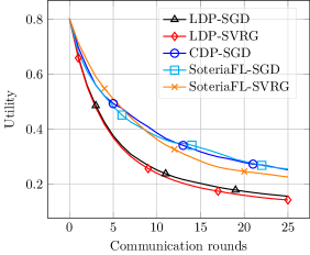
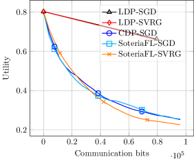
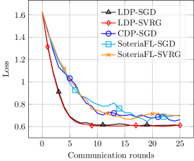
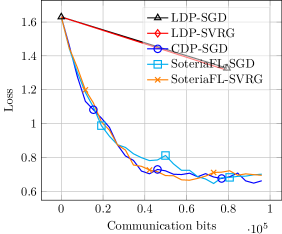
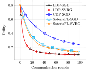
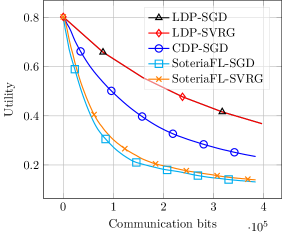
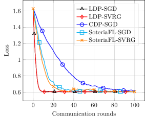
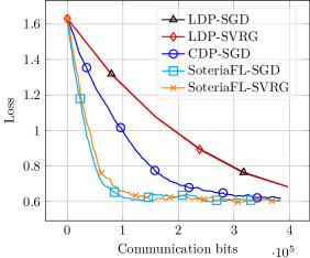
Figure 1: Logistic regression with nonconvex regularization on the a9a dataset under ($\epsilon,\delta$)-LDP with $\epsilon=1$ and $\delta=10^{-3}$. The top (resp. bottom) row is for utility (resp. training loss) vs. communication rounds and communication bits.

Figure 2: Logistic regression with nonconvex regularization on the a9a dataset under ($\epsilon,\delta$)-LDP with $\epsilon=5$ and $\delta=10^{-3}$. The top (resp. bottom) row is for utility (resp. training loss) vs. communication rounds and communication bits.

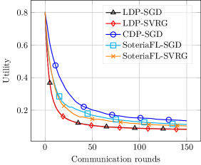
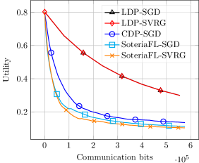
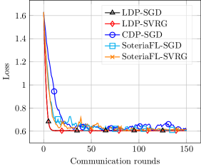
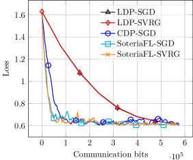
Figure 3: Logistic regression with nonconvex regularization on the a9a dataset under ($\epsilon,\delta$)-LDP with $\epsilon=10$ and $\delta=10^{-3}$. The top (resp. bottom) row is for utility (resp. training loss) vs. communication rounds and communication bits.

Remark.

From the experimental results, it can be seen that the two uncompressed algorithms (LDP-SGD and LDP-SVRG) converge faster than the three compressed algorithms (CDP-SGD, SoteriaFL-SGD, SoteriaFL-SVRG) in terms of communication rounds (see left columns in each figure). However, in terms of communication bits (see right columns in each figure), compressed algorithms perform better than the uncompressed algorithms. This validates that communication compression indeed provide significant savings in terms of communication cost. The figures also confirm that shifted compression based SoteriaFL typically performs better than direct compression based CDP-SGD in both utility and training loss. For SoteriaFL-style algorithms, it turns out that SoteriaFL-SVRG performs slightly better than SoteriaFL-SGD in the utility (see top rows in each figure). This is quite consistent with our theoretical results.

6.2 Shallow neural network training

We consider a simple 1-hidden layer neural network training task, with $64$ hidden neurons, sigmoid activation functions, and the cross-entropy loss. The objective function over a data sample $({\bm{a}},b)$ is defined as

$$f({\bm{x}};({\bm{a}},b))=\ell(\mathsf{softmax}(\bm{W}_{2}~{}\mathsf{sigmoid}(\bm{W}_{1}{\bm{a}}+\bm{c}_{1})+\bm{c}_{2}),b),$$

where $\ell(\cdot,\cdot)$ denotes the cross-entropy loss, the optimization variable is collectively denoted by ${\bm{x}}=\text{vec}(\bm{W}_{1},\bm{c}_{1},\bm{W}_{2},\bm{c}_{2})$, with the dimensions of the network parameters $\bm{W}_{1}$, $\bm{c}_{1}$, $\bm{W}_{2}$, $\bm{c}_{2}$ being $64\times 784$, $64\times 1$, $10\times 64$, and $10\times 1$, respectively. Here, we run the experiments on the standard MNIST dataset [44]. To demonstrate the privacy-utility-communication trade-offs, we consider five levels of $(\epsilon,\delta)$-LDP with $\epsilon=1,2,4,8,16$ and a common $\delta=10^{-3}$, where the experimental results are reported in Figures 5–8, respectively.

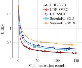
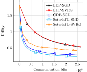
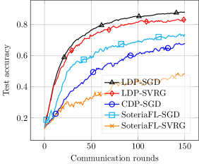
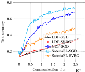
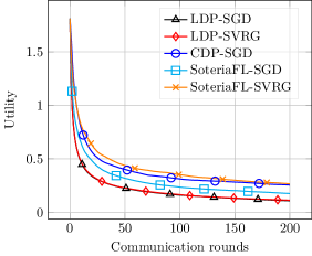
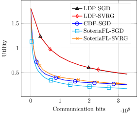
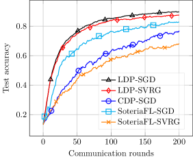
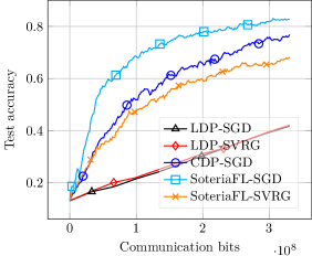
Figure 4: Shallow neural network training on the MNIST dataset under ($\epsilon,\delta$)-LDP with $\epsilon=1$ and $\delta=10^{-3}$. The top (resp. bottom) row is for utility (resp. test accuracy) vs. communication rounds and communication bits.

Figure 5: Shallow neural network training on the MNIST dataset under ($\epsilon,\delta$)-LDP with $\epsilon=2$ and $\delta=10^{-3}$. The top (resp. bottom) row is for utility (resp. test accuracy) vs. communication rounds and communication bits.

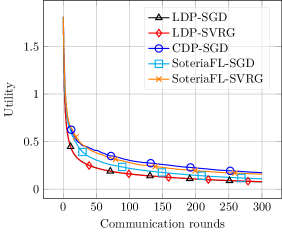
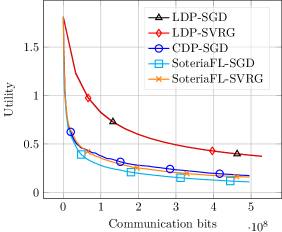
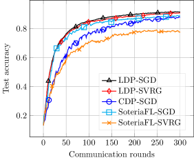
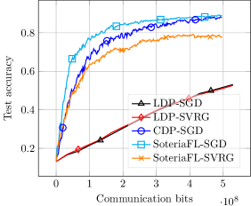
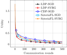
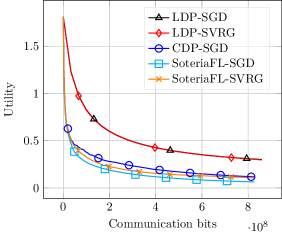
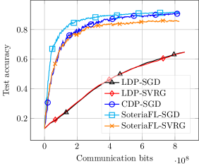
Figure 6: Shallow neural network training on the MNIST dataset under ($\epsilon,\delta$)-LDP with $\epsilon=4$ and $\delta=10^{-3}$. The top (resp. bottom) row is for utility (resp. test accuracy) vs. communication rounds and communication bits.

Figure 7: Shallow neural network training on the MNIST dataset under ($\epsilon,\delta$)-LDP with $\epsilon=8$ and $\delta=10^{-3}$. The top (resp. bottom) row is for utility (resp. test accuracy) vs. communication rounds and communication bits.

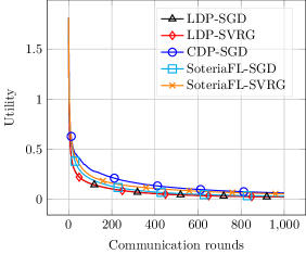
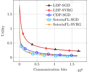
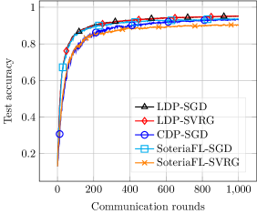
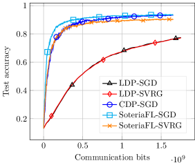
Figure 8: Shallow neural network training on the MNIST dataset under ($\epsilon,\delta$)-LDP with $\epsilon=16$ and $\delta=10^{-3}$. The top (resp. bottom) row is for utility (resp. test accuracy) vs. communication rounds and communication bits.

Remark.

Note that here we report the test accuracy for training the neural network instead of the training loss as earlier (see bottom rows in Figures 5–8 vs. in Figures 2–3). The takeaways from the experimental results are similar to previous experiments on logistic regression with nonconvex regularization (Figures 2–3). Again, the two uncompressed algorithms (LDP-SGD and LDP-SVRG) converge faster than the three compressed algorithms (CDP-SGD, SoteriaFL-SGD, SoteriaFL-SVRG) in terms of communication rounds (see left columns in each figure), but the gap becomes smaller when the privacy level $\epsilon$ gets larger (i.e. less privacy guarantee). However, in terms of communication bits (see right columns in each figure), compressed algorithms again perform much better than the uncompressed algorithms, validating the advantage of communication compression schemes. Last but not least, shifted compression based SoteriaFL-SGD performs better than direct compression based CDP-SGD in both utility and test accuracy. However, it turns out that SoteriaFL-SVRG may perform worse than CDP-SGD for training this shallow neural network.

7 Conclusion

We propose SoteriaFL, a unified framework for private FL, which accommodates a general family of local gradient estimators including popular stochastic variance-reduced gradient methods and the state-of-the-art shifted compression scheme. A unified characterization of its performance trade-offs in terms of privacy, utility (convergence accuracy), and communication complexity is presented, which is then instantiated to arrive at several new private FL algorithms. All of these algorithms are shown to perform better than the plain CDP-SGD algorithm especially when the local dataset size is large, and have lower communication complexity compared with other private FL algorithms without compression.

Appendix

We now provide all missing proofs. Concretely, Appendix A and B provide the detailed proofs for our unified privacy guarantee in Theorem 2 and unified utility and communication complexity analysis in Theorem 3, respectively. Appendix C provides the proof for CDP-SGD (Theorem 1). Finally, Appendix D provides the proofs for Section 5, including Lemma 1 (showing that several local gradient estimators satisfy the generic Assumption 3) and Corollaries 1–3 (instantiating Lemma 1 in the unified Theorem 3) for the proposed SoteriaFL-style algorithms.

Appendix A Proof of Theorem 2

In the proof of Theorem 2, we apply a moment argument (similar to [1]) to prove the local differential privacy guarantees. Before going into the detailed proof, we first define some concepts.

Moment generating function.

Assume that there is a mechanism ${\mathcal{M}}:{\mathcal{D}}\to{\mathcal{R}}$. For neighboring datasets $D,D^{\prime}\in{\mathcal{D}}$, a mechanism ${\mathcal{M}}$, auxiliary inputs aux, and an outcome $o\in{\mathcal{R}}$, we define the private loss at $o$ as

$$c(o;{\mathcal{M}},\text{aux},D,D^{\prime}):=\log\frac{\Pr\{{\mathcal{M}}(\text{aux},D)=o\}}{\Pr\{{\mathcal{M}}(\text{aux},D^{\prime})=o\}}.$$

We also define

$$\alpha^{{\mathcal{M}}}(\lambda;\text{aux},D,D^{\prime}):=\log\mathbb{E}_{o\sim{\mathcal{M}}(\text{aux},D)}\left[\exp\left(\lambda\cdot c(o;{\mathcal{M}},\text{aux},D,D^{\prime})\right)\right]$$

and

$$\alpha_{i}^{{\mathcal{M}}}(\lambda):=\max_{\text{aux},D,D^{\prime}}\alpha^{{\mathcal{M}}}(\lambda;\text{aux},D,D^{\prime}),$$

where $D=(D_{-i},D_{i}),D^{\prime}=(D_{-i},D^{\prime}_{i})$ are neighboring datasets that differ only at client $i$, $D_{-i}$ denoting all the data at clients other than client $i$. We call $\alpha^{{\mathcal{M}}}(\lambda;\text{aux},D,D^{\prime})$ and $\alpha_{i}^{{\mathcal{M}}}(\lambda)$ the log moment generating functions.

Sub-mechanisms.

We assume that there are $n\times T$ sub-mechanisms $\{{\mathcal{M}}_{i}^{t}\}_{i\in[n],t\leq T}$ in ${\mathcal{M}}$, where ${\mathcal{M}}_{i}^{t}$ corresponds to the mechanism for client $i$ in round $t$. We further let ${\mathcal{M}}_{i}^{t}:={\mathcal{A}}\circ\overline{{\mathcal{M}}}_{i}^{t}$ be the composition of mechanism $\overline{{\mathcal{M}}}_{i}^{t}$ and the mechanism ${\mathcal{A}}$. Here, ${\mathcal{A}}:{\mathcal{R}}\to{\mathcal{R}}$ is a random mechanism that maps an outcome to another outcome, and $\overline{{\mathcal{M}}}_{i}^{t}$ is possibly an adaptive mechanism that takes the input of all the outputs before time $t$, i.e. $o_{i}^{s}$ for all $s<t$ and $i\in[n]$. We assume that given all the previous outcomes $o_{i}^{s}$ for $s<t$, the random mechanisms $\overline{{\mathcal{M}}}_{i}^{t}$ for all $i\in[n]$ are independent w.r.t. each other (this is satisfied in SoteriaFL). In SoteriaFL (Algorithm 2), ${\mathcal{A}}$ corresponds to the compression step, and $\overline{{\mathcal{M}}}_{i}^{t}$ corresponds the Gaussian perturbation.

Before proving Theorem 2, we first state the following result from [1].

Proposition 1 (Theorem 2 in [1]).

For any $\epsilon>0$, the mechanism ${\mathcal{M}}$ is $(\epsilon,\delta)$-LDP for client $i$ with $\delta=\min_{\lambda}\exp\left(\alpha_{i}^{{\mathcal{M}}}(\lambda)-\lambda\epsilon\right)$.

According to Proposition 1, we know that if the log moment generating function $\alpha_{i}^{{\mathcal{M}}}(\lambda)$ is bounded, then we can show that the mechanism ${\mathcal{M}}$ satisfies $(\epsilon,\delta)$-LDP with some parameters $\epsilon$ and $\delta$. To prove that the log moment generating function $\alpha_{i}^{{\mathcal{M}}}(\lambda)$ is bounded, we divide it into two parts: 1) the log moment generating function $\alpha_{i}^{{\mathcal{M}}}(\lambda)$ for the whole mechanism can be bounded by the summation of the log moment generating function of all sub mechanisms $\alpha_{i}^{\overline{{\mathcal{M}}}_{i}^{t}}(\lambda)$ from $t=1$ to $T$; and 2) the log moment generating function for each sub mechanism is bounded, i.e. $\alpha_{i}^{\overline{{\mathcal{M}}}_{i}^{t}}(\lambda)$ is bounded. To this end, we provide the following two lemmas to formalize these two parts respectively.

Lemma 2 (Privacy for composition).

For any client $i$ and any $\lambda$, the following holds

$$\alpha_{i}^{{\mathcal{M}}}(\lambda)\leq\sum_{t=1}^{T}\alpha^{\overline{{\mathcal{M}}}_{i}^{t}}(\lambda).$$

Lemma 3 (Privacy for sub mechanism).

Suppose that Assumption 2 and 3 are satisfied. For any client $i$, let $\sigma_{p}\geq 1$ and let ${\mathcal{I}}_{b}$ be a random minibatch from local dataset $D_{i}=\{d_{i,j}\}_{j=1}^{m}$ where each data sample $d_{i,j}$ is chosen independently with probability $q=\frac{b}{m}<\frac{G_{A}}{16b\sigma_{p}}$. Then for any positive integer $\lambda\leq\frac{2b^{2}\sigma_{p}^{2}}{3G_{A}^{2}}\log\frac{G_{A}}{qb\sigma_{p}}$, the sub mechanism $\overline{{\mathcal{M}}}_{i}^{t}$ satisfies

$$\alpha^{\overline{{\mathcal{M}}}_{i}^{t}}(\lambda)\leq\frac{6\lambda(\lambda+1)(G_{A}^{2}/4+G_{B}^{2})}{(1-q)m^{2}\sigma_{p}^{2}}+O\left(\frac{q^{3}\lambda^{3}}{\sigma_{p}^{3}}\right).$$

The detailed proofs for Lemmas 2 and 3 are provided in Appendix A.1 and A.2, respectively.

Proof of Theorem 2.

Now, we are ready to prove our privacy guarantee in Theorem 2 using Proposition 1, and Lemmas 2 and 3.

Proof of Theorem 2.

Assume for now that $\sigma_{p},\lambda$ satisfy the conditions in Lemma 3, namely

$$\lambda\leq\frac{2b^{2}\sigma_{p}^{2}}{3G_{A}^{2}}\log\frac{G_{A}}{q\sigma_{p}b}.$$ (7)

By Lemmas 3 and 2, there exists some constant $\hat{c}$ such that for small enough $q$, the log moment generating function of Algorithm 2 can be bounded as follows

$$\alpha_{i}^{{\mathcal{M}}}(\lambda)\leq\hat{c}\frac{T\lambda^{2}(G_{A}^{2}/4+G_{B}^{2})}{m^{2}\sigma_{p}^{2}},\qquad\forall i\in[n].$$

Combining the above bound and Proposition 1, to guarantee Algorithm 2 to be $(\epsilon,\delta)$-LDP, it suffices to establish that there exists some $\lambda$ that satisfies (7) and the following two conditions:

$$\hat{c}\frac{T\lambda^{2}(G_{A}^{2}/4+G_{B}^{2})}{m^{2}\sigma_{p}^{2}} \leq\frac{\lambda\epsilon}{2}\qquad\mbox{or equivalently}\quad\lambda\leq\frac{\epsilon m^{2}\sigma_{p}^{2}}{2\hat{c}T(G_{A}^{2}/4+G_{B}^{2})},$$ (8)

$$\exp\left(-\frac{\lambda\epsilon}{2}\right) \leq\delta\qquad\mbox{or equivalently}\quad\lambda\geq\frac{2}{\epsilon}\log\frac{1}{\delta}.$$ (9)

It is now easy to verify that when $\epsilon=c^{\prime}q^{2}T$ for some constant $c^{\prime}$, we can satisfy all these conditions by setting

$$\sigma_{p}^{2}=c\frac{(G_{A}^{2}/4+G_{B}^{2})T\log(1/\delta)}{m^{2}\epsilon^{2}}$$

for some constant $c$. ∎

A.1 Proof of Lemma 2

Before embarking on the proof of Lemma 2, we begin with an observation that connects the log moment generation function with the Rényi divergence of distributions $\Pr\{{\mathcal{M}}(\text{aux},D)=o\}$ and $\Pr\{{\mathcal{M}}(\text{aux},D^{\prime})=o\}$.

Lemma 4.

Denote the Rényi divergence between any two distributions ${\mathcal{P}}$ and ${\mathcal{Q}}$ with parameter $\lambda+1$ as

$$D_{\lambda+1}^{\text{R\'{e}nyi}}({\mathcal{P}}\|{\mathcal{Q}})=\frac{1}{\lambda}\log\mathbb{E}_{{\mathcal{P}}}\left(\frac{\textup{{d}}{\mathcal{P}}}{\textup{{d}}{\mathcal{Q}}}\right)^{\lambda}.$$

Then, the log moment generating function has the following form

$$\alpha^{{\mathcal{M}}}(\lambda;\text{aux},D,D^{\prime})=\lambda D^{\text{R\'{e}nyi}}_{\lambda+1}\left({\mathcal{M}}(\text{aux},D)\|{\mathcal{M}}(\text{aux},D^{\prime})\right).$$ (10)

Proof of Lemma 4.

By direct computation, we have

$$\alpha^{{\mathcal{M}}}(\lambda;\text{aux},D,D^{\prime}) =\log\mathbb{E}_{o\sim{\mathcal{M}}(\text{aux},D)}\left[\exp\left(\lambda\cdot c(o;{\mathcal{M}},\text{aux},D,D^{\prime})\right)\right]$$

$$=\log\mathbb{E}_{o\sim{\mathcal{M}}(\text{aux},D)}\left[\exp\left(\lambda\cdot\log\frac{\Pr\{{\mathcal{M}}(\text{aux},D)=o\}}{\Pr\{{\mathcal{M}}(\text{aux},D^{\prime})=o\}}\right)\right]$$

$$=\log\mathbb{E}_{o\sim{\mathcal{M}}(\text{aux},D)}\left[\left(\frac{\Pr\{{\mathcal{M}}(\text{aux},D)=o\}}{\Pr\{{\mathcal{M}}(\text{aux},D^{\prime})=o\}}\right)^{\lambda}\right]$$

$$=\lambda D^{\text{R\'{e}nyi}}_{\lambda+1}\left({\mathcal{M}}(\text{aux},D)\|{\mathcal{M}}(\text{aux},D^{\prime})\right).$$

∎

We will also need the following data processing inequality for Rényi divergence.

Lemma 5 (Data processing inequality for Rényi divergence [68]).

Let ${\mathcal{P}},{\mathcal{Q}}$ be two distributions over ${\mathcal{R}}$, ${\mathcal{S}}:{\mathcal{R}}\to{\mathcal{R}}$ be a random mapping, and $D^{\text{R\'{e}nyi}}_{\lambda}$ denote the Rényi Divergence, then we have

$$D^{\text{R\'{e}nyi}}_{\lambda+1}({\mathcal{S}}({\mathcal{P}})\|{\mathcal{S}}({\mathcal{Q}}))\leq D^{\text{R\'{e}nyi}}_{\lambda+1}({\mathcal{P}}\|{\mathcal{Q}}),$$

where ${\mathcal{S}}({\mathcal{P}})$ stands for the resulting distribution of applying random mapping ${\mathcal{S}}$ on distribution ${\mathcal{P}}$.

Proof of Lemma 2.

We divide the proof of Lemma 2 into two steps: 1) $\alpha_{i}^{{\mathcal{M}}}(\lambda)\leq\sum_{t=1}^{T}\alpha^{{\mathcal{M}}_{i}^{t}}(\lambda)$; and 2) $\alpha^{{\mathcal{M}}_{i}^{t}}(\lambda)\leq\alpha^{\overline{{\mathcal{M}}}_{i}^{t}}(\lambda)$. Combining these two steps directly leads to the declared bound, namely

$$\alpha_{i}^{{\mathcal{M}}}(\lambda) \leq\sum_{t=1}^{T}\alpha^{{\mathcal{M}}_{i}^{t}}(\lambda)\leq\sum_{t=1}^{T}\alpha^{\overline{{\mathcal{M}}}_{i}^{t}}(\lambda).$$

The rest of this proof is thus dedicated to establishing the two steps. For simplicity, we use $o_{1:n}^{1:T}$ to denote the outcomes $\{o_{i}^{t}\}_{i\in[n],t\in[T]}$, and ${\mathcal{M}}_{1:n}^{1:T}$ to denote the mechanisms $\{{\mathcal{M}}^{t}_{i}\}_{i\in[n],t\in[T]}$.

Step 1: establishing $\alpha_{i}^{{\mathcal{M}}}(\lambda)\leq\sum_{t=1}^{T}\alpha^{{\mathcal{M}}_{i}^{t}}(\lambda)$.

For neighboring datasets $D=(D_{-i},D_{i}),D^{\prime}=(D_{-i},D^{\prime}_{i})$ that differ only on client $i$, we have

$$c(o_{1:n}^{1:T};{\mathcal{M}}_{1:n}^{1:T},o_{1:n}^{1:T-1},D,D^{\prime}) =\log\frac{\Pr\{{\mathcal{M}}_{1:n}^{1:T}(o_{1:n}^{1:T-1},D)=o_{1:n}^{1:T}\}}{\Pr\{{\mathcal{M}}_{1:n}^{1:T}(o_{1:n}^{1:T-1},D^{\prime})=o_{1:n}^{1:T}\}}$$

$$=\log\prod_{t=1}^{T}\prod_{j=1}^{n}\frac{\Pr\{{\mathcal{M}}_{j}^{t}(o_{1:n}^{1:T-1},D)=o_{j}^{t}\}}{\Pr\{{\mathcal{M}}_{j}^{t}(o_{1:n}^{1:T-1},D^{\prime})=o_{j}^{t}\}}$$

$$=\log\prod_{t=1}^{T}\frac{\Pr\{{\mathcal{M}}_{i}^{t}(o_{1:n}^{1:T-1},D)=o_{i}^{t}\}}{\Pr\{{\mathcal{M}}_{i}^{t}(o_{1:n}^{1:T-1},D^{\prime})=o_{i}^{t}\}}$$

$$=\sum_{t=1}^{T}\log\frac{\Pr\{{\mathcal{M}}_{i}^{t}(o_{1:n}^{1:T-1},D)=o_{i}^{t}\}}{\Pr\{{\mathcal{M}}_{i}^{t}(o_{1:n}^{1:T-1},D^{\prime})=o_{i}^{t}\}}$$

$$=\sum_{t=1}^{T}c(o_{i}^{t};{\mathcal{M}}_{i}^{t},o_{1:n}^{1:T-1},D,D^{\prime}).$$

Here, the second line comes from the fact that the mechanisms of different clients at the same round are independent, and the third line comes from the fact that for any client $j\neq i$, $D_{j}=D^{\prime}_{j}$, and thus $\frac{\Pr\{{\mathcal{M}}_{j}^{t}(o_{1:n}^{1:T-1},D)=o_{j}^{t}\}}{\Pr\{{\mathcal{M}}_{j}^{t}(o_{1:n}^{1:T-1},D^{\prime})=o_{j}^{t}\}}=1$. Then we have

$$\mathbb{E}_{o_{1:n}^{1:T}\sim{\mathcal{M}}_{1:n}^{1:T}}\left[\exp\left(\lambda c(o_{1:n}^{1:T};{\mathcal{M}}_{1:n}^{1:T},o_{1:n}^{1:T-1},D,D^{\prime})\right)\right] =\mathbb{E}_{o_{1:n}^{1:T}\sim{\mathcal{M}}_{1:n}^{1:T}}\left[\exp\left(\lambda\sum_{t=1}^{T}c(o_{i}^{t};{\mathcal{M}}_{i}^{t},o_{1:n}^{1:T-1},D,D^{\prime})\right)\right]$$

$$=\mathbb{E}_{o_{1:n}^{1:T}\sim{\mathcal{M}}_{1:n}^{1:T}}\left[\prod_{t=1}^{T}\exp\left(\lambda c(o_{i}^{t};{\mathcal{M}}_{i}^{t},o_{1:n}^{1:T-1},D,D^{\prime})\right)\right]$$

$$=\prod_{t=1}^{T}\mathbb{E}_{o_{1:n}^{1:T}\sim{\mathcal{M}}_{1:n}^{1:T}}\left[\exp\left(\lambda c(o_{i}^{t};{\mathcal{M}}_{i}^{t},o_{1:n}^{1:T-1},D,D^{\prime})\right)\right]$$

$$=\prod_{t=1}^{T}\exp\left(\alpha^{{\mathcal{M}}_{i}^{t}}(\lambda;o_{1:n}^{1:T-1},D,D^{\prime})\right)$$

$$=\exp\left(\sum_{t=1}^{T}\alpha^{{\mathcal{M}}_{i}^{t}}(\lambda;o_{1:n}^{1:T-1},D,D^{\prime})\right).$$

Taking logarithm on both sides and maximizing over $o_{1:n}^{1:T-1},D,D^{\prime}$, we can show that

$$\alpha_{i}^{{\mathcal{M}}}(\lambda)\leq\sum_{t=1}^{T}\alpha^{{\mathcal{M}}_{i}^{t}}(\lambda).$$

Step 2: establishing $\alpha^{{\mathcal{M}}_{i}^{t}}(\lambda)\leq\alpha^{\overline{{\mathcal{M}}}_{i}^{t}}(\lambda)$.

This step follows directly from Lemma 5. Namely, for fixed $i$ and $t$, we can compute

$$\alpha^{{\mathcal{M}}_{i}^{t}}(\lambda;o_{1:n}^{1:T-1},D,D^{\prime}) =\lambda D^{\text{R\'{e}nyi}}_{\lambda+1}\left({\mathcal{M}}_{i}^{t}(o_{1:n}^{1:T-1},D)\|{\mathcal{M}}_{i}^{t}(o_{1:n}^{1:T-1},D^{\prime})\right)$$

$$=\lambda D^{\text{R\'{e}nyi}}_{\lambda+1}\left(({\mathcal{A}}\circ\overline{{\mathcal{M}}}_{i}^{t})(o_{1:n}^{1:T-1},D)\|({\mathcal{A}}\circ\overline{{\mathcal{M}}}_{i}^{t})(o_{1:n}^{1:T-1},D^{\prime})\right)$$

$$\leq\lambda D^{\text{R\'{e}nyi}}_{\lambda+1}\left(\overline{{\mathcal{M}}}_{i}^{t}(o_{1:n}^{1:T-1},D)\|\overline{{\mathcal{M}}}_{i}^{t}(o_{1:n}^{1:T-1},D^{\prime})\right)$$

$$=\alpha^{\overline{{\mathcal{M}}}_{i}^{t}}(\lambda;o_{1:n}^{1:T-1},D,D^{\prime}).$$

Then, taking the maximum over $o_{1:n}^{1:T-1},D,D^{\prime}$, we have

$$\alpha^{{\mathcal{M}}_{i}^{t}}(\lambda)\leq\alpha^{\overline{{\mathcal{M}}}_{i}^{t}}(\lambda).$$

∎

A.2 Proof of Lemma 3

It is worth noting that the proof does not requires $f({\bm{x}};d_{i,j})$ to be a function with respect to the data sample $d_{i,j}$ at point ${\bm{x}}$, it can be any function related to $d_{i,j}$, for example, $\phi_{i,j}$ in Assumption 3. Inspired by [69], we decompose the gradient estimator into two parts and bound the privacy respectively. Now we provide the detailed proofs below.

Proof of Lemma 3.

From Assumption 3, we first write out and decouple the sub-mechanism $\overline{{\mathcal{M}}}_{i}^{t}$ (corresponding to the Gaussian perturbation) as

$$\frac{1}{b}\sum_{j\in{\mathcal{I}}_{b}}\varphi_{i,j}^{t}+\frac{1}{m}\sum_{j=1}^{m}\psi_{i,j}^{t}+{\bm{\xi}}_{i}^{t}=\left(\frac{1}{b}\sum_{j\in{\mathcal{I}}_{b}}\varphi_{i,j}^{t}+{\bm{\xi}}_{i,1}^{t}\right)+\left(\frac{1}{m}\sum_{j=1}^{m}\psi_{i,j}^{t}+{\bm{\xi}}_{i,2}^{t}\right),$$ (11)

where ${\bm{\xi}}_{i}^{t}$ is generated from ${\mathcal{N}}(0,\sigma_{p}^{2}{\bm{I}})$ and ${\bm{\xi}}_{i,1}^{t},{\bm{\xi}}_{2,1}^{t}$ are generated from ${\mathcal{N}}(0,\frac{2\sigma_{p}^{2}}{3}{\bm{I}})$, ${\mathcal{N}}(0,\frac{\sigma_{p}^{2}}{3}{\bm{I}})$ independently. Now, $\overline{{\mathcal{M}}}_{i}^{t}$ can be viewed as a composition of two mechanisms $\overline{{\mathcal{M}}}_{i,1}^{t}$ and $\overline{{\mathcal{M}}}_{i,2}^{t}$, where $\overline{{\mathcal{M}}}_{i,1}^{t}$ denote the first term and $\overline{{\mathcal{M}}}_{i,2}^{t}$ denote the second term in the right-hand-side (RHS) of (11). From [1, Theorem 2.1], we have

$$\alpha^{\overline{{\mathcal{M}}}_{i}^{t}}(\lambda)\leq\alpha^{\overline{{\mathcal{M}}}_{i,1}^{t}}(\lambda)+\alpha^{\overline{{\mathcal{M}}}_{i,2}^{t}}(\lambda).$$ (12)

For the first term of (12), according to [1, Lemma 3], we have

$$\alpha^{\overline{{\mathcal{M}}}_{i,1}^{t}}(\lambda)\leq\frac{3\lambda(\lambda+1)G_{A}^{2}}{2(1-q)m^{2}\sigma_{p}^{2}}+O\left(\frac{q^{3}\lambda^{3}}{\sigma_{p}^{3}}\right),$$ (13)

for $q=\frac{b}{m}<\frac{G_{A}}{16\sigma_{p}b}$ and any positive integer $\lambda\leq\frac{2b^{2}\sigma_{p}^{2}}{3G_{A}^{2}}\log\frac{G_{A}}{q\sigma_{p}b}$, where we set $\sigma^{2}$ in [1, Lemma 3] to be $\frac{2b^{2}\sigma_{p}^{2}}{3G_{A}^{2}}$.

For the second term of (12), according to Lemma 4 (the relationship between Rényi divergence and the moment generating function), we have

$$\alpha^{\overline{{\mathcal{M}}}_{i,2}^{t}}(\lambda)=\lambda D_{\lambda+1}^{\text{R\'{e}nyi}}({\mathcal{P}}\|{\mathcal{Q}}),$$ (14)

where ${\mathcal{P}}=\frac{1}{m}\sum_{j=1}^{m}\psi_{i,j}^{t}+{\mathcal{N}}(0,\frac{2\sigma_{p}^{2}}{3}{\bm{I}})$ and ${\mathcal{Q}}=\frac{1}{m}\sum_{j=1}^{m}(\psi_{i,j}^{t})^{\prime}+{\mathcal{N}}(0,\frac{\sigma_{p}^{2}}{3}{\bm{I}})$. Here, $\{\psi_{i,j}^{t},\;j\in[m]\}$ contains the functions corresponding to the data in dataset $D$, and $\{(\psi_{i,j}^{t})^{\prime},\;j\in[m]\}$ contains the functions corresponding to the data in dataset $D^{\prime}$. We note that all functions except one in $\{\psi_{i,j}^{t},\;j\in[m]\}$ and $\{(\psi_{i,j}^{t})^{\prime},\;j\in[m]\}$ are the same, since the datasets $D$ and $D^{\prime}$ only differ by one element. According to [8, Lemma 17], we have

$$\lambda D_{\lambda+1}^{\text{R\'{e}nyi}}({\mathcal{P}}\|{\mathcal{Q}})=\frac{3\lambda(\lambda+1)\left\|\frac{1}{m}\sum_{j=1}^{m}\psi_{i,j}^{t}-\frac{1}{m}\sum_{j=1}^{m}(\psi_{i,j}^{t})^{\prime}\right\|^{2}}{2\sigma_{p}^{2}}\leq\frac{6\lambda(\lambda+1)G_{B}^{2}}{m^{2}\sigma_{p}^{2}}.$$ (15)

The proof is finished by combining (12)–(15). ∎

Appendix B Proof of Theorem 3

We now provide the detailed proofs for our unified Theorem 3. First, according to the update rule ${\bm{x}}^{t+1}={\bm{x}}^{t}-\eta_{t}{{\bm{v}}^{t}}$ (Line 9 in Algorithm 2) and the smoothness assumption (Assumption 1), we have

$$\mathbb{E}_{t}[f({\bm{x}}^{t+1})]\leq\mathbb{E}_{t}\left[f({\bm{x}}^{t})-\eta_{t}\langle\nabla f({\bm{x}}^{t}),{{\bm{v}}^{t}}\rangle+\frac{L\eta_{t}^{2}}{2}\|{{\bm{v}}^{t}}\|^{2}\right],$$ (16)

where $\mathbb{E}_{t}$ takes the expectation conditioned on all history before round $t$. To begin, we show that ${{\bm{v}}^{t}}$ is unbiased as follows:

$$\mathbb{E}_{t}[{{\bm{v}}^{t}}]=\mathbb{E}_{t}\left[{\bm{s}}^{t}+\frac{1}{n}\sum_{i=1}^{n}{{\bm{v}}_{i}^{t}}\right] =\mathbb{E}_{t}\left[\frac{1}{n}\sum_{i=1}^{n}{{\bm{s}}_{i}^{t}}+\frac{1}{n}\sum_{i=1}^{n}{\cal C}_{i}^{t}({\bm{g}}_{i}^{t}-{{\bm{s}}_{i}^{t}})\right]$$

$$=\mathbb{E}_{t}\left[\frac{1}{n}\sum_{i=1}^{n}{\bm{g}}_{i}^{t}\right]=\mathbb{E}_{t}\left[\frac{1}{n}\sum_{i=1}^{n}(\tilde{{\bm{g}}}_{i}^{t}+{\bm{\xi}}_{i}^{t})\right]$$ (17)

$$=\mathbb{E}_{t}\left[\frac{1}{n}\sum_{i=1}^{n}\tilde{{\bm{g}}}_{i}^{t}\right]$$ (18)

$$=\mathbb{E}_{t}\left[\frac{1}{n}\sum_{i=1}^{n}\nabla f_{i}({\bm{x}}^{t})\right]=\nabla f({\bm{x}}^{t}),$$ (19)

where (17) follows from (2), (18) holds due to ${\bm{\xi}}_{i}^{t}\sim{\mathcal{N}}(\bm{0},\sigma_{p}^{2}{\bm{I}})$, and (19) is due to $\mathbb{E}_{t}[\tilde{{\bm{g}}}_{i}^{t}]=\nabla f_{i}({\bm{x}}^{t})$ from Assumption 3.

Plugging (18) into (16), we get

$$\mathbb{E}_{t}[f({\bm{x}}^{t+1})]\leq\mathbb{E}_{t}\left[f({\bm{x}}^{t})-\eta_{t}\|\nabla f({\bm{x}}^{t})\|^{2}+\frac{L\eta_{t}^{2}}{2}\|{{\bm{v}}^{t}}\|^{2}\right].$$ (20)

We then bound the last term $\mathbb{E}_{t}[\|{{\bm{v}}^{t}}\|^{2}]$ in the follow lemma, whose proof is provided in Appendix B.1.

Lemma 6.

Suppose that ${{\bm{v}}^{t}}$ is defined and computed in Algorithm 2, we have

$$\mathbb{E}_{t}[\|{{\bm{v}}^{t}}\|^{2}] \leq\mathbb{E}_{t}\left[\frac{(1+\omega)}{n^{2}}\sum_{i=1}^{n}\|\tilde{{\bm{g}}}_{i}^{t}-\nabla f_{i}({\bm{x}}^{t})\|^{2}\right]+\frac{\omega}{n^{2}}\sum_{i=1}^{n}\|\nabla f_{i}({\bm{x}}^{t})-{{\bm{s}}_{i}^{t}}\|^{2}+\|\nabla f({\bm{x}}^{t})\|^{2}+\frac{(1+\omega)d{\sigma_{p}^{2}}}{n}.$$ (21)

To continue, we need to bound the first two terms in (21). The first term can be controlled via (3b) of Assumption 3. Now we show that the second term will shrink in the following lemma, whose proof is provided in Appendix B.2.

Lemma 7.

Suppose that Assumption 1 holds and the shift ${\bm{s}}_{i}^{t+1}$ is defined and computed in Algorithm 2. Then letting $\gamma_{t}=\sqrt{\frac{1+2\omega}{2(1+\omega)^{3}}}$, we have

$$\mathbb{E}_{t}\left[\frac{1}{n}\sum_{i=1}^{n}\|\nabla f_{i}({\bm{x}}^{t+1})-{\bm{s}}_{i}^{t+1}\|^{2}\right] \leq\mathbb{E}_{t}\bigg{[}\Big{(}1-\frac{1}{2(1+\omega)}\Big{)}\frac{1}{n}\sum_{i=1}^{n}\left\|\nabla f_{i}({\bm{x}}^{t})-{{\bm{s}}_{i}^{t}}\right\|^{2}$$

$$\qquad\quad+\frac{1}{(1+\omega)n}\sum_{i=1}^{n}\|\tilde{{\bm{g}}}_{i}^{t}-\nabla f_{i}({\bm{x}}^{t})\|^{2}$$

$$\qquad\quad+2(1+\omega)L^{2}\left\|{\bm{x}}^{t+1}-{\bm{x}}^{t}\right\|^{2}+\frac{d{\sigma_{p}^{2}}}{1+\omega}\Big{)}\bigg{]}.$$ (22)

To facilitate presentation, let us introduce the short-hand notation ${\mathcal{S}}^{t}:=\frac{1}{n}\sum_{i=1}^{n}\|\nabla f_{i}({\bm{x}}^{t})-{{\bm{s}}_{i}^{t}}\|^{2}$. Then we define the following potential function

$$\Phi_{t}:=f({\bm{x}}^{t})-f^{*}+\alpha L\Delta^{t}+\frac{\beta}{L}{\mathcal{S}}^{t},$$ (23)

for some $\alpha\geq 0,\beta\geq 0$. With the help of Lemmas 6 and 7, we show that this potential function decreases in each round in the following lemma, whose proof is provided in Appendix B.3.

Lemma 8.

Under Assumptions 1 and 3, if we choose the stepsize as

$$\eta_{t}\equiv\eta\leq\min\left\{\frac{1}{(1+2\alpha C_{4}+4\beta(1+\omega)+2\alpha C_{3}/\eta^{2})L},\frac{\sqrt{\beta n}}{\sqrt{1+2\alpha C_{4}+4\beta(1+\omega)}(1+\omega)L}\right\},$$

where $\alpha=\frac{3\beta C_{1}}{2(1+\omega)\theta L^{2}}$, $\forall\beta>0$, and the shift stepsize as $\gamma_{t}\equiv\sqrt{\frac{1+2\omega}{2(1+\omega)^{3}}}$, then we have for any round $t\geq 0$,

$$\mathbb{E}_{t}[\Phi_{t+1}]\leq\Phi_{t}-\frac{\eta_{t}}{2}\|\nabla f({\bm{x}}^{t})\|^{2}+\frac{3\beta}{2(1+\omega)L}(C_{2}+d{\sigma_{p}^{2}}).$$ (24)

Given Lemma 8 and Theorem 2, now we are ready to prove Theorem 3 regarding the utility and communication complexity for SoteriaFL.

Proof of Theorem 3.

First, we sum up (24) (Lemma 8) from round $t=0$ to $T-1$,

$$\sum_{t=0}^{T-1}\frac{\eta_{t}}{2}\mathbb{E}\|\nabla f({\bm{x}}^{t})\|^{2} \leq\Phi_{0}+\frac{3\beta}{2(1+\omega)L}\left(C_{2}+d{\sigma_{p}^{2}}\right)T.$$ (25)

Then by choosing the stepsize $\eta_{t}$ as in Lemma 8 and the privacy variance ${\sigma_{p}^{2}}=\frac{c(G_{A}^{2}/4+G_{B}^{2})T\log(1/\delta))}{m^{2}\epsilon^{2}}$ according to Theorem 2, we obtain

$$\frac{1}{T}\sum_{t=0}^{T-1}\mathbb{E}\|\nabla f({\bm{x}}^{t})\|^{2} \leq\frac{2\Phi_{0}}{\eta T}+\frac{3\beta}{(1+\omega)L\eta}\left(C_{2}+\frac{c(G_{A}^{2}/4+G_{B}^{2})dT\log({1}/{\delta})}{m^{2}\epsilon^{2}}\right),$$ (26)

and SoteriaFL (Algorithm 2) satisfies $(\epsilon,\delta)$-LDP.

Finally, the total number of communication rounds $T$ in (5) comes from the following relations in RHS of (26)

$$\frac{2\Phi_{0}}{\eta T} \leq\frac{3\beta}{(1+\omega)L\eta}\frac{c(G_{A}^{2}/4+G_{B}^{2})dT\log({1}/{\delta})}{m^{2}\epsilon^{2}},$$

$$C_{2} \leq\frac{c(G_{A}^{2}/4+G_{B}^{2})dT\log({1}/{\delta})}{m^{2}\epsilon^{2}}.$$

The utility guarantee (6) directly follows from (26) by choosing $T$ as in (5). ∎

B.1 Proof of Lemma 6

According to the definition of ${{\bm{v}}^{t}}$, we have

$$\mathbb{E}_{t}[\|{{\bm{v}}^{t}}\|^{2}] =\mathbb{E}_{t}\left[\left\|\frac{1}{n}\sum_{i=1}^{n}{{\bm{s}}_{i}^{t}}+\frac{1}{n}\sum_{i=1}^{n}{\cal C}_{i}^{t}({\bm{g}}_{i}^{t}-{{\bm{s}}_{i}^{t}})\right\|^{2}\right]$$

$$=\mathbb{E}_{t}\left[\left\|\frac{1}{n}\sum_{i=1}^{n}{\cal C}_{i}^{t}({\bm{g}}_{i}^{t}-{{\bm{s}}_{i}^{t}})-\frac{1}{n}\sum_{i=1}^{n}({\bm{g}}_{i}^{t}-{{\bm{s}}_{i}^{t}})+\frac{1}{n}\sum_{i=1}^{n}{\bm{g}}_{i}^{t}\right\|^{2}\right]$$

$$\leq\mathbb{E}_{t}\left[\frac{\omega}{n^{2}}\sum_{i=1}^{n}\|{\bm{g}}_{i}^{t}-{{\bm{s}}_{i}^{t}}\|^{2}\right]+\mathbb{E}_{t}\left[\left\|\frac{1}{n}\sum_{i=1}^{n}{\bm{g}}_{i}^{t}\right\|^{2}\right],$$ (27)

where the last line is due to the definition of the compression operator (2). To continue, we bound each term in (27) respectively.

• For the first term, we have

  $$\mathbb{E}_{t}\left[\frac{\omega}{n^{2}}\sum_{i=1}^{n}\|{\bm{g}}_{i}^{t}-{{\bm{s}}_{i}^{t}}\|^{2}\right] =\mathbb{E}_{t}\left[\frac{\omega}{n^{2}}\sum_{i=1}^{n}\|\tilde{{\bm{g}}}_{i}^{t}-{{\bm{s}}_{i}^{t}}+{\bm{\xi}}_{i}^{t}\|^{2}\right]$$

  $$=\mathbb{E}_{t}\left[\frac{\omega}{n^{2}}\sum_{i=1}^{n}(\|\tilde{{\bm{g}}}_{i}^{t}-{{\bm{s}}_{i}^{t}}\|^{2}+d{\sigma_{p}^{2}})\right]$$

  $$=\mathbb{E}_{t}\left[\frac{\omega}{n^{2}}\sum_{i=1}^{n}\|\tilde{{\bm{g}}}_{i}^{t}-{{\bm{s}}_{i}^{t}}\|^{2}\right]+\frac{\omega d{\sigma_{p}^{2}}}{n}$$

  $$=\mathbb{E}_{t}\left[\frac{\omega}{n^{2}}\sum_{i=1}^{n}\|\tilde{{\bm{g}}}_{i}^{t}-\nabla f_{i}({\bm{x}}^{t})+\nabla f_{i}({\bm{x}}^{t})-{{\bm{s}}_{i}^{t}}\|^{2}\right]+\frac{\omega d{\sigma_{p}^{2}}}{n}$$

  $$=\mathbb{E}_{t}\left[\frac{\omega}{n^{2}}\sum_{i=1}^{n}\|\tilde{{\bm{g}}}_{i}^{t}-\nabla f_{i}({\bm{x}}^{t})\|^{2}\right]+\frac{\omega}{n^{2}}\sum_{i=1}^{n}\|\nabla f_{i}({\bm{x}}^{t})-{{\bm{s}}_{i}^{t}}\|^{2}+\frac{\omega d{\sigma_{p}^{2}}}{n},$$ (28)

  where the last line is due to $\mathbb{E}_{t}[\tilde{{\bm{g}}}_{i}^{t}]=\nabla f_{i}({\bm{x}}^{t})$ from Assumption 3.

• Similarly, for the second term, we have

  $$\mathbb{E}_{t}\left[\left\|\frac{1}{n}\sum_{i=1}^{n}{\bm{g}}_{i}^{t}\right\|^{2}\right] =\mathbb{E}_{t}\left[\left\|\frac{1}{n}\sum_{i=1}^{n}(\tilde{{\bm{g}}}_{i}^{t}+{\bm{\xi}}_{i}^{t})\right\|^{2}\right]$$

  $$=\mathbb{E}_{t}\left[\left\|\frac{1}{n}\sum_{i=1}^{n}\tilde{{\bm{g}}}_{i}^{t}\right\|^{2}+\frac{d{\sigma_{p}^{2}}}{n}\right]$$

  $$=\mathbb{E}_{t}\left[\left\|\frac{1}{n}\sum_{i=1}^{n}(\tilde{{\bm{g}}}_{i}^{t}-\nabla f_{i}({\bm{x}}^{t})+\nabla f_{i}({\bm{x}}^{t}))\right\|^{2}\right]+\frac{d{\sigma_{p}^{2}}}{n}$$

  $$=\mathbb{E}_{t}\left[\frac{1}{n^{2}}\sum_{i=1}^{n}\|\tilde{{\bm{g}}}_{i}^{t}-\nabla f_{i}({\bm{x}}^{t})\|^{2}\right]+\|\nabla f({\bm{x}}^{t})\|^{2}+\frac{d{\sigma_{p}^{2}}}{n}.$$ (29)

The proof is completed by plugging (28) and (29) into (27).

B.2 Proof of Lemma 7

According to the shift update (Line 6 in Algorithm 2), we have

$$\mathbb{E}_{t}\left[\frac{1}{n}\sum_{i=1}^{n}\|\nabla f_{i}({\bm{x}}^{t+1})-{\bm{s}}_{i}^{t+1}\|^{2}\right]$$

$$=\mathbb{E}_{t}\left[\frac{1}{n}\sum_{i=1}^{n}\left\|\nabla f_{i}({\bm{x}}^{t+1})-{{\bm{s}}_{i}^{t}}-\gamma_{t}{\cal C}_{i}^{t}({\bm{g}}_{i}^{t}-{{\bm{s}}_{i}^{t}})\right\|^{2}\right]$$

$$=\mathbb{E}_{t}\left[\frac{1}{n}\sum_{i=1}^{n}\left\|\nabla f_{i}({\bm{x}}^{t+1})-\nabla f_{i}({\bm{x}}^{t})+\nabla f_{i}({\bm{x}}^{t})-{{\bm{s}}_{i}^{t}}-\gamma_{t}{\cal C}_{i}^{t}({\bm{g}}_{i}^{t}-{{\bm{s}}_{i}^{t}})\right\|^{2}\right]$$

$$\leq\mathbb{E}_{t}\bigg{[}\frac{1}{n}\sum_{i=1}^{n}\Big{(}(1+\frac{1}{\beta_{t}})\left\|\nabla f_{i}({\bm{x}}^{t+1})-\nabla f_{i}({\bm{x}}^{t})\right\|^{2}+(1+\beta_{t})\left\|\nabla f_{i}({\bm{x}}^{t})-{{\bm{s}}_{i}^{t}}-\gamma_{t}{\cal C}_{i}^{t}({\bm{g}}_{i}^{t}-{{\bm{s}}_{i}^{t}})\right\|^{2}\Big{)}\bigg{]}$$ (30)

$$\leq\mathbb{E}_{t}\bigg{[}(1+\frac{1}{\beta_{t}})L^{2}\left\|{\bm{x}}^{t+1}-{\bm{x}}^{t}\right\|^{2}+(1+\beta_{t})\frac{1}{n}\sum_{i=1}^{n}\left\|\nabla f_{i}({\bm{x}}^{t})-{{\bm{s}}_{i}^{t}}-\gamma_{t}{\cal C}_{i}^{t}({\bm{g}}_{i}^{t}-{{\bm{s}}_{i}^{t}})\right\|^{2}\bigg{]},$$ (31)

where (30) uses Young’s inequality with any $\beta_{t}>0$ (its choice will be specified momentarily), and (31) uses Assumption 1. The second term of (31) can be further bounded as follows:

$$\mathbb{E}_{t}\left[\frac{1}{n}\sum_{i=1}^{n}\left\|\nabla f_{i}({\bm{x}}^{t})-{{\bm{s}}_{i}^{t}}-\gamma_{t}{\cal C}_{i}^{t}({\bm{g}}_{i}^{t}-{{\bm{s}}_{i}^{t}})\right\|^{2}\right]$$

$$=\mathbb{E}_{t}\bigg{[}\frac{1}{n}\sum_{i=1}^{n}\Big{(}(1-2\gamma_{t})\left\|\nabla f_{i}({\bm{x}}^{t})-{{\bm{s}}_{i}^{t}}\right\|^{2}+\gamma_{t}^{2}\|{\cal C}_{i}^{t}({\bm{g}}_{i}^{t}-{{\bm{s}}_{i}^{t}})\|^{2}\Big{)}\bigg{]}$$

$$\overset{(\ref{eq:comp})}{\leq}\mathbb{E}_{t}\bigg{[}\frac{1}{n}\sum_{i=1}^{n}\Big{(}(1-2\gamma_{t})\left\|\nabla f_{i}({\bm{x}}^{t})-{{\bm{s}}_{i}^{t}}\right\|^{2}+\gamma_{t}^{2}(1+\omega)\|{\bm{g}}_{i}^{t}-{{\bm{s}}_{i}^{t}}\|^{2}\Big{)}\bigg{]}$$

$$=\mathbb{E}_{t}\bigg{[}\frac{1}{n}\sum_{i=1}^{n}\Big{(}\big{(}1-2\gamma_{t}+\gamma_{t}^{2}(1+\omega)\big{)}\left\|\nabla f_{i}({\bm{x}}^{t})-{{\bm{s}}_{i}^{t}}\right\|^{2}+\gamma_{t}^{2}(1+\omega)\|\tilde{{\bm{g}}}_{i}^{t}-\nabla f_{i}({\bm{x}}^{t})\|^{2}+\gamma_{t}^{2}(1+\omega)d{\sigma_{p}^{2}}\Big{)}\bigg{]},$$ (32)

where the first equality follows from

$$\mathbb{E}_{t}\left[\left\langle\nabla f_{i}({\bm{x}}^{t})-{{\bm{s}}_{i}^{t}},\,{\cal C}_{i}^{t}({\bm{g}}_{i}^{t}-{{\bm{s}}_{i}^{t}})\right\rangle\right]=\mathbb{E}_{t}\left[\left\|\nabla f_{i}({\bm{x}}^{t})-{{\bm{s}}_{i}^{t}}\right\|^{2}\right],$$

and the last line follows from (28). The proof is completed by plugging (32) into (31) and choosing $\beta_{t}=\frac{1}{1+2\omega}$ and $\gamma_{t}=\sqrt{\frac{1+2\omega}{2(1+\omega)^{3}}}$.

B.3 Proof of Lemma 8

Recalling ${\mathcal{S}}^{t}:=\frac{1}{n}\sum_{i=1}^{n}\|\nabla f_{i}({\bm{x}}^{t})-{{\bm{s}}_{i}^{t}}\|^{2}$, ${\mathcal{S}}^{t}$ can be recursively bounded by Lemma 7 as

$$\mathbb{E}_{t}[{\mathcal{S}}^{t+1}] \leq\mathbb{E}_{t}\bigg{[}\big{(}1-\frac{1}{2(1+\omega)}\big{)}{\mathcal{S}}^{t}+\frac{1}{(1+\omega)n}\sum_{i=1}^{n}\|\tilde{{\bm{g}}}_{i}^{t}-\nabla f_{i}({\bm{x}}^{t})\|^{2}$$

$$\qquad\qquad+2(1+\omega)L^{2}\left\|{\bm{x}}^{t+1}-{\bm{x}}^{t}\right\|^{2}+\frac{d{\sigma_{p}^{2}}}{1+\omega}\bigg{]}.$$ (33)

Note that the second term can be bounded by (3b) of Assumption 3, namely

$$\mathbb{E}_{t}\Big{[}\frac{1}{n}\sum_{i=1}^{n}\|\tilde{{\bm{g}}}_{i}^{t}-\nabla f_{i}({\bm{x}}^{t})\|^{2}\Big{]}\leq C_{1}\Delta^{t}+C_{2},$$

leading to

$$\mathbb{E}_{t}[{\mathcal{S}}^{t+1}] \leq\mathbb{E}_{t}\bigg{[}\big{(}1-\frac{1}{2(1+\omega)}\big{)}{\mathcal{S}}^{t}+\frac{C_{1}\Delta^{t}+C_{2}}{(1+\omega)n}+2(1+\omega)L^{2}\left\|{\bm{x}}^{t+1}-{\bm{x}}^{t}\right\|^{2}+\frac{d{\sigma_{p}^{2}}}{1+\omega}\bigg{]}.$$

Combined with (20), we can bound the potential function (23) as

$$\mathbb{E}_{t}[\Phi_{t+1}] :=\mathbb{E}_{t}\left[f({\bm{x}}^{t+1})-f^{*}+\alpha L\Delta^{t+1}+\frac{\beta}{L}{\mathcal{S}}^{t+1}\right]$$

$$\leq\mathbb{E}_{t}\bigg{[}f({\bm{x}}^{t})-f^{*}-\eta_{t}\|\nabla f({\bm{x}}^{t})\|^{2}+\frac{L\eta_{t}^{2}}{2}\|{{\bm{v}}^{t}}\|^{2}+\alpha L\Delta^{t+1}$$

$$\qquad\qquad+\frac{\beta}{L}\Big{(}\big{(}1-\frac{1}{2(1+\omega)}\big{)}{\mathcal{S}}^{t}+\frac{C_{1}\Delta^{t}+C_{2}}{1+\omega}+2(1+\omega)L^{2}\left\|{\bm{x}}^{t+1}-{\bm{x}}^{t}\right\|^{2}+\frac{d{\sigma_{p}^{2}}}{1+\omega}\Big{)}\bigg{]}$$

$$\overset{(\ref{ass:var-Delta})}{\leq}\mathbb{E}_{t}\bigg{[}f({\bm{x}}^{t})-f^{*}-\eta_{t}\|\nabla f({\bm{x}}^{t})\|^{2}+\frac{L\eta_{t}^{2}}{2}\|{{\bm{v}}^{t}}\|^{2}$$

$$\qquad\qquad+\alpha L\Big{(}(1-\theta)\Delta^{t}+C_{3}\|\nabla f({\bm{x}}^{t})\|^{2}+C_{4}\|{\bm{x}}^{t+1}-{\bm{x}}^{t}\|^{2}\Big{)}$$

$$\qquad\qquad+\frac{\beta}{L}\Big{(}\big{(}1-\frac{1}{2(1+\omega)}\big{)}{\mathcal{S}}^{t}+\frac{C_{1}\Delta^{t}+C_{2}}{1+\omega}+2(1+\omega)L^{2}\left\|{\bm{x}}^{t+1}-{\bm{x}}^{t}\right\|^{2}+\frac{d{\sigma_{p}^{2}}}{1+\omega}\Big{)}\bigg{]}$$

$$=\mathbb{E}_{t}\bigg{[}f({\bm{x}}^{t})-f^{*}-\eta_{t}\|\nabla f({\bm{x}}^{t})\|^{2}+\Big{(}\frac{1}{2}+\alpha C_{4}+2\beta(1+\omega)\Big{)}L\eta_{t}^{2}\|{{\bm{v}}^{t}}\|^{2}$$

$$\qquad\qquad+\alpha L\Big{(}(1-\theta)\Delta^{t}+C_{3}\|\nabla f({\bm{x}}^{t})\|^{2}\Big{)}$$

$$\qquad\qquad+\frac{\beta}{L}\Big{(}\big{(}1-\frac{1}{2(1+\omega)}\big{)}{\mathcal{S}}^{t}+\frac{C_{1}\Delta^{t}+C_{2}}{1+\omega}+\frac{d{\sigma_{p}^{2}}}{1+\omega}\Big{)}\bigg{]},$$ (34)

where the last line follows from the update rule ${\bm{x}}^{t+1}={\bm{x}}^{t}-\eta_{t}{{\bm{v}}^{t}}$ (Line 9 of Algorithm 2). To continue, we invoke Lemma 6, which gives

$$\mathbb{E}_{t}[\|{{\bm{v}}^{t}}\|^{2}] \leq\mathbb{E}_{t}\left[\frac{(1+\omega)}{n^{2}}\sum_{i=1}^{n}\|\tilde{{\bm{g}}}_{i}^{t}-\nabla f_{i}({\bm{x}}^{t})\|^{2}+\frac{\omega}{n}{\mathcal{S}}^{t}+\|\nabla f({\bm{x}}^{t})\|^{2}+\frac{(1+\omega)d{\sigma_{p}^{2}}}{n}\right]$$

$$\leq\mathbb{E}_{t}\left[\frac{(1+\omega)}{n}C_{1}\Delta^{t}+\frac{\omega}{n}{\mathcal{S}}^{t}+\|\nabla f({\bm{x}}^{t})\|^{2}+\frac{(1+\omega)(C_{2}+d{\sigma_{p}^{2}})}{n}\right],$$

where the second line uses again (3b) of Assumption 3. Plugging this back into (34), we arrive at

$$\mathbb{E}_{t}[\Phi_{t+1}] \leq f({\bm{x}}^{t})-f^{*}+\bigg{[}\alpha(1-\theta)+\frac{\beta C_{1}}{(1+\omega)L^{2}}+\Big{(}\frac{1}{2}+\alpha C_{4}+2\beta(1+\omega)\Big{)}\frac{(1+\omega)C_{1}\eta_{t}^{2}}{n}\bigg{]}L\Delta^{t}$$

$$\qquad\qquad+\bigg{[}\beta\big{(}1-\frac{1}{2(1+\omega)}\big{)}+\Big{(}\frac{1}{2}+\alpha C_{4}+2\beta(1+\omega)\Big{)}\frac{\omega L^{2}\eta_{t}^{2}}{n}\bigg{]}\frac{{\mathcal{S}}^{t}}{L}$$

$$\qquad\qquad-\bigg{[}\eta_{t}-\alpha LC_{3}-\Big{(}\frac{1}{2}+\alpha C_{4}+2\beta(1+\omega)\Big{)}L\eta_{t}^{2}\bigg{]}\|\nabla f({\bm{x}}^{t})\|^{2}$$

$$\qquad\qquad+\bigg{[}\frac{\beta}{(1+\omega)L}+\Big{(}\frac{1}{2}+\alpha C_{4}+2\beta(1+\omega)\Big{)}\frac{(1+\omega)L\eta_{t}^{2}}{n}\bigg{]}(C_{2}+d{\sigma_{p}^{2}}).$$ (35)

Now we choose the appropriate parameters satisfying

$$\alpha(1-\theta)+\frac{\beta C_{1}}{(1+\omega)L^{2}}+\Big{(}\frac{1}{2}+\alpha C_{4}+2\beta(1+\omega)\Big{)}\frac{(1+\omega)C_{1}\eta_{t}^{2}}{n} \leq\alpha,$$ (36)

$$\beta\big{(}1-\frac{1}{2(1+\omega)}\big{)}+\Big{(}\frac{1}{2}+\alpha C_{4}+2\beta(1+\omega)\Big{)}\frac{\omega L^{2}\eta_{t}^{2}}{n} \leq\beta,$$ (37)

so that the RHS of (35) can lead to the potential function $\Phi_{t}:=f({\bm{x}}^{t})-f^{*}+\alpha L\Delta^{t}+\frac{\beta}{L}{\mathcal{S}}^{t}$. It is not hard to verify that the following choice of $\alpha,\beta,\eta_{t}$ satisfy (36) and (37):

$$\alpha\geq\frac{3\beta C_{1}}{2(1+\omega)L^{2}\theta},\qquad\forall\beta>0,$$ (38)

$$\eta_{t}\equiv\eta\leq\frac{\sqrt{\beta n}}{\sqrt{1+2\alpha C_{4}+4\beta(1+\omega)}(1+\omega)L}.$$ (39)

Note that (39) implies

$$\Big{(}\frac{1}{2}+\alpha C_{4}+2\beta(1+\omega)\Big{)}\frac{(1+\omega)\eta_{t}^{2}}{n}\leq\frac{\beta}{2(1+\omega)L^{2}}.$$ (40)

If we further choose the stepsize

$$\eta_{t}\equiv\eta\leq\frac{1}{(1+2\alpha C_{4}+4\beta(1+\omega)+2\alpha C_{3}/\eta^{2})L},$$ (41)

then the proof is finished by combining (35)–(41) since (35) simplifies to

$$\mathbb{E}_{t}[\Phi_{t+1}]\leq\Phi_{t}-\frac{\eta_{t}}{2}\|\nabla f({\bm{x}}^{t})\|^{2}+\frac{3\beta}{2(1+\omega)L}(C_{2}+d{\sigma_{p}^{2}}).$$

Appendix C Proof of Theorem 1

We now give the detailed proof for Theorem 1. We first show the privacy guarantee of CDP-SGD and then derive the utility guarantee.

C.1 Privacy guarantee of CDP-SGD

Theorem 4 (Privacy guarantee for CDP-SGD).

Suppose Assumption 2 holds. There exist constants $c^{\prime}$ and $c$ so that given the sampling probability $q=b/m$ and the number of steps $T$, for any $\epsilon<c^{\prime}q^{2}T$ and $\delta\in(0,1)$, CDP-SGD (Algorithm 1) is $(\epsilon,\delta)$-LDP if we choose

$$\sigma_{p}^{2}=c\frac{G^{2}T\log(1/\delta)}{m^{2}\epsilon^{2}}.$$

The proof of Theorem 4 is very similar to the proof of Theorem 2. Thus here we just point out some differences between the proof of Theorem 4 and 2.

Sub-mechanisms.

Similar to Theorem 2, we define the sub-mechanisms in the following way. We assume that there are $n\times T$ sub-mechanisms $\{{\mathcal{M}}_{i}^{t}\}_{i\in[n],t\leq T}$ in ${\mathcal{M}}$, where ${\mathcal{M}}_{i}^{t}$ corresponds to the mechanism for client $i$ in round $t$. We further let ${\mathcal{M}}_{i}^{t}:={\mathcal{A}}\circ\overline{{\mathcal{M}}}_{i}^{t}$ be the composition of mechanism $\overline{{\mathcal{M}}}_{i}^{t}$ and the mechanism ${\mathcal{A}}$. Here, ${\mathcal{A}}:{\mathcal{R}}\to{\mathcal{R}}$ is a random mechanism that maps an outcome to another outcome, and $\overline{{\mathcal{M}}}_{i}^{t}$ is possibly an adaptive mechanism that takes the input of all the outputs before time $t$, i.e. $o_{i}^{s}$ for all $s<t$ and $i\in[n]$. We assume that given all the previous outcomes $o_{i}^{s}$ for $s<t$, the random mechanisms $\overline{{\mathcal{M}}}_{i}^{t}$ for all $i\in[n]$ are independent w.r.t. each other (this is satisfied in CDP-SGD). In CDP-SGD (Algorithm 1), ${\mathcal{A}}$ corresponds to the compression operator, and $\overline{{\mathcal{M}}}_{i}^{t}$ corresponds the Gaussian perturbation. The difference between the sub-mechanisms for SoteriaFL and CDP-SGD is the presence of the shift. However as the shift is known to the central server, we can omit that during the analysis of privacy.

Privacy for composition (Lemma 2).

Here CDP-SGD can use exactly the same previous Lemma 2 since the relationship between the final mechanism and the sub-mechanism does not change.

Privacy for sub-mechanisms (Lemma 3).

The privacy guarantee for sub-mechanisms of Theorem 4 is simpler than that for Theorem 2, since we can simply apply Lemma 3 of [1] to obtain the following bound

$$\alpha^{\overline{{\mathcal{M}}}_{i}^{t}}(\lambda)\leq\frac{\lambda(\lambda+1)G^{2}}{(1-q)m^{2}\sigma_{p}^{2}}+O\left(\frac{q^{3}\lambda^{3}}{\sigma_{p}^{3}}\right).$$

C.2 Utility guarantee of CDP-SGD

To prove the convergence result, we first give the following lemma providing the mean and variance of the stochastic gradient $\tilde{{\bm{g}}}_{i}^{t}=\frac{1}{b}\sum_{j\in{\mathcal{I}}_{b}}\nabla f_{i,j}({\bm{x}}^{t})$ (Line 4 in Algorithm 1).

Lemma 9 (Variance).

Under Assumption 2, for any client $i$, the stochastic gradient estimator $\tilde{{\bm{g}}}_{i}^{t}=\frac{1}{b}\sum_{j\in{\mathcal{I}}_{b}}\nabla f_{i,j}({\bm{x}}^{t})$ is unbiased, i.e.

$$\mathbb{E}_{t}\Bigg{[}\frac{1}{b}\sum_{j\in{\mathcal{I}}_{b}}\nabla f_{i,j}({\bm{x}}^{t})\Bigg{]}=\nabla f_{i}({\bm{x}}^{t}),$$

where $\mathbb{E}_{t}$ takes the expectation conditioned on all history before round $t$. Also, we have

$$\mathbb{E}_{t}\left[\left\|\frac{1}{b}\sum_{j\in{\mathcal{I}}_{b}}\nabla f_{i,j}({\bm{x}}^{t})-\nabla f_{i}({\bm{x}}^{t})\right\|^{2}\right]\leq\frac{(1-q)G^{2}}{b},$$ (42)

where $q=b/m$.

Proof.

We first show that the estimator is unbiased. Define $m$ independent Bernoulli random variables $X_{i,j}$, where $\Pr\{X_{i,j}=1\}=q=\frac{b}{m}$. Then,

$$\mathbb{E}_{t}\Bigg{[}\frac{1}{b}\sum_{j\in{\mathcal{I}}_{b}}\nabla f_{i,j}({\bm{x}}^{t})\Bigg{]}=\mathbb{E}_{t}\Bigg{[}\frac{1}{b}\sum_{j=1}^{m}X_{i,j}\nabla f_{i,j}({\bm{x}}^{t})\Bigg{]}=\frac{1}{m}\sum_{j=1}^{m}\nabla f_{i,j}({\bm{x}}^{t})=\nabla f_{i}({\bm{x}}^{t}).$$

Moving onto the variance bound, we have

$$\mathbb{E}_{t}\left[\left\|\frac{1}{b}\sum_{j\in{\mathcal{I}}_{b}}\nabla f_{i,j}({\bm{x}}^{t})-\nabla f_{i}({\bm{x}}^{t})\right\|^{2}\right] =\mathbb{E}_{t}\left[\left\|\frac{1}{b}\sum_{j=1}^{m}X_{i,j}\nabla f_{i,j}({\bm{x}}^{t})-\nabla f_{i}({\bm{x}}^{t})\right\|^{2}\right]$$

$$=\mathbb{E}_{t}\left[\left\|\sum_{j=1}^{m}\left(\frac{1}{b}X_{i,j}\nabla f_{i,j}({\bm{x}}^{t})-\frac{1}{m}\nabla f_{i,j}({\bm{x}}^{t})\right)\right\|^{2}\right]$$

$$=\mathbb{E}_{t}\left[\sum_{j=1}^{m}\left\|\frac{1}{b}(X_{i,j}-q)\nabla f_{i,j}({\bm{x}}^{t})\right\|^{2}\right]$$ (43)

$$=\sum_{j=1}^{m}\frac{(1-q)q}{b^{2}}\left\|\nabla f_{i,j}({\bm{x}}^{t})\right\|^{2}\leq\frac{(1-q)G^{2}}{b},$$

where (43) comes from the fact that random variables $X_{i,j}$ are independent, and the last line follows from the variance of Bernoulli random variables as well as Assumption 2. ∎

With the help of the above lemma, we now prove Theorem 1.

Proof of Theorem 1.

First, from the smoothness Assumption 1, we have

$$f({\bm{x}}^{t+1})\leq f({\bm{x}}^{t})-\eta_{t}\left<\nabla f({\bm{x}}^{t}),{\bm{v}}^{t}\right>+\frac{L\eta_{t}^{2}}{2}\left\|{\bm{v}}^{t}\right\|^{2}.$$

Taking the expectation on both sides of the above inequality, we have (note that we choose constant stepsize $\eta_{t}\equiv\eta$ for simplicity)

$$\mathbb{E}_{t}[f({\bm{x}}^{t+1})]\leq f({\bm{x}}^{t})-\eta\mathbb{E}_{t}\left<\nabla f({\bm{x}}^{t}),{\bm{v}}^{t}\right>+\frac{L\eta^{2}}{2}\mathbb{E}_{t}\left\|{\bm{v}}^{t}\right\|^{2}.$$ (44)

To control $\mathbb{E}_{t}\left<\nabla f({\bm{x}}^{t}),{\bm{v}}^{t}\right>$, notice that

$$\mathbb{E}_{t}\left<\nabla f({\bm{x}}^{t}),{\bm{v}}^{t}\right>=\mathbb{E}_{t}\left<\nabla f({\bm{x}}^{t}),\frac{1}{n}\sum_{i=1}^{n}{\bm{v}}_{i}^{t}\right> =\mathbb{E}_{t}\left<\nabla f({\bm{x}}^{t}),\frac{1}{n}\sum_{i=1}^{n}{\mathcal{C}}_{i}^{t}({\bm{g}}_{i}^{t})\right>$$

$$\overset{(\ref{eq:comp})}{=}\mathbb{E}_{t}\left<\nabla f({\bm{x}}^{t}),\frac{1}{n}\sum_{i=1}^{n}{\bm{g}}_{i}^{t}\right>$$

$$=\mathbb{E}_{t}\left<\nabla f({\bm{x}}^{t}),\frac{1}{n}\sum_{i=1}^{n}(\tilde{{\bm{g}}}_{i}^{t}+{\bm{\xi}}_{i}^{t})\right>$$

$$=\left\|\nabla f({\bm{x}}^{t})\right\|^{2},$$

where the last line follows from Lemma 9 as well as the independence of the added Gaussian perturbation. Next, using the definition ${\bm{v}}_{i}^{t}={\mathcal{C}}_{i}^{t}({\bm{g}}_{i}^{t})$ and the properties of the compression operator, we compute $\mathbb{E}_{t}\left\|{\bm{v}}^{t}\right\|^{2}$ as follows,

$$\mathbb{E}_{t}\left\|{\bm{v}}^{t}\right\|^{2} =\mathbb{E}_{t}\left\|\frac{1}{n}\sum_{i=1}^{n}{\bm{v}}_{i}^{t}\right\|^{2}$$

$$=\mathbb{E}_{t}\left[\left\|\frac{1}{n}\sum_{i=1}^{n}({\bm{v}}_{i}^{t}-{\bm{g}}_{i}^{t})\right\|^{2}+\left\|\frac{1}{n}\sum_{i=1}^{n}{\bm{g}}_{i}^{t}\right\|^{2}\right]$$

$$\overset{(\ref{eq:comp})}{\leq}\mathbb{E}_{t}\left[\frac{1}{n^{2}}\sum_{i=1}^{n}\omega\left\|{\bm{g}}_{i}^{t}\right\|^{2}+\left\|\frac{1}{n}\sum_{i=1}^{n}{\bm{g}}_{i}^{t}\right\|^{2}\right]$$

$$\leq\frac{1}{n^{2}}\sum_{i=1}^{n}\omega\left(\left\|\nabla f_{i}({\bm{x}}^{t})\right\|^{2}+\frac{(1-q)\mathbb{E}_{t}\left\|\tilde{{\bm{g}}}_{i}^{t}-\nabla f_{i}({\bm{x}}^{t})\right\|^{2}}{b}+d\sigma_{p}^{2}\right)$$

$$\quad\quad+\left\|\nabla f({\bm{x}}^{t})\right\|^{2}+\frac{(1-q)\mathbb{E}_{t}\left\|\tilde{{\bm{g}}}_{i}^{t}-\nabla f_{i}({\bm{x}}^{t})\right\|^{2}}{bn}+\frac{d\sigma_{p}^{2}}{n}$$

$$\overset{(\ref{eq:variance})}{\leq}\frac{1}{n^{2}}\sum_{i=1}^{n}\omega\left(\left\|\nabla f_{i}({\bm{x}}^{t})\right\|^{2}+\frac{(1-q)G^{2}}{b}+d\sigma_{p}^{2}\right)+\left\|\nabla f({\bm{x}}^{t})\right\|^{2}+\frac{(1-q)G^{2}}{bn}+\frac{d\sigma_{p}^{2}}{n}$$

$$~{}\leq\left\|\nabla f({\bm{x}}^{t})\right\|^{2}+\frac{1}{n}\left(\omega G^{2}+(1+\omega)\frac{(1-q)G^{2}}{b}+(1+\omega)d\sigma_{p}^{2}\right),$$ (45)

where the last inequality (45) follows from Assumption 2.

Plugging the above two relations back to (44), we obtain

$$\mathbb{E}_{t}[f({\bm{x}}^{t+1})]\leq f({\bm{x}}^{t})-\left(\eta-\frac{L\eta^{2}}{2}\right)\left\|\nabla f({\bm{x}}^{t})\right\|^{2}+\frac{L\eta^{2}}{2n}\left(\omega G^{2}+(1+\omega)\frac{(1-q)G^{2}}{b}+(1+\omega)d\sigma_{p}^{2}\right).$$

By choosing $\eta\leq\frac{1}{L}$, we have

$$\mathbb{E}_{t}[f({\bm{x}}^{t+1})]\leq f({\bm{x}}^{t})-\frac{\eta}{2}\left\|\nabla f({\bm{x}}^{t})\right\|^{2}+\frac{L\eta^{2}}{2n}\left(\omega G^{2}+(1+\omega)\frac{(1-q)G^{2}}{b}+(1+\omega)d\sigma_{p}^{2}\right).$$

Plugging in $\sigma_{p}$ (Theorem 4), telescoping over the iterations $t=1,\ldots,T$, and rearranging terms, we can prove

$$\frac{1}{T}\sum_{t=1}^{T}\mathbb{E}\left\|\nabla f({\bm{x}}^{t})\right\|^{2} \leq\frac{2(f({\bm{x}}^{0})-f^{*})}{\eta T}+\frac{L\eta}{n}\left[\omega G^{2}+(1+\omega)\frac{(1-q)G^{2}}{b}+\frac{(1+\omega)cdG^{2}T\log(1/\delta)}{m^{2}\epsilon^{2}}\right]$$

$$\leq\frac{2D_{f}}{\eta T}+\frac{L\eta}{n}\left[\frac{(1+\omega+\omega b)}{b}G^{2}+\frac{(1+\omega)cdG^{2}T\log(1/\delta)}{m^{2}\epsilon^{2}}\right],$$ (46)

where we use the notation $D_{f}:=f({\bm{x}}^{0})-f^{*}$. We choose $T$ and $\eta$ to satisfy

$$\eta T=\frac{m\epsilon\sqrt{nD_{f}}}{G\sqrt{L(1+\omega)cd\log(1/\delta)}},\quad T\geq\frac{m^{2}\epsilon^{2}}{cd\log\left(1/\delta\right)}.$$ (47)

According to the relation (47) and stepsize $\eta\leq\frac{1}{L}$, we set $T=\max\Big{\{}\frac{m\epsilon\sqrt{nLD_{f}}}{G\sqrt{(1+\omega)cd\log(1/\delta)}},\frac{m^{2}\epsilon^{2}}{cd\log(1/\delta)}\Big{\}}$ and $\eta=\min\Big{\{}\frac{1}{L},\frac{\sqrt{nD_{f}cd\log(1/\delta)}}{Gm\epsilon\sqrt{(1+\omega)L}}\Big{\}}$. Then (46) turns out as

$$\frac{1}{T}\sum_{t=1}^{T}\mathbb{E}\left\|\nabla f({\bm{x}}^{t})\right\|^{2} \leq\frac{2D_{f}}{\eta T}+\frac{L\eta}{n}\left[2(1+\omega)G^{2}+\frac{(1+\omega)cdG^{2}T\log(1/\delta)}{m^{2}\epsilon^{2}}\right]$$

$$\overset{(\ref{eq:T-cdpsgd})}{\leq}\frac{2D_{f}}{\eta T}+\frac{L\eta}{n}\cdot\frac{3(1+\omega)cdG^{2}T\log(1/\delta)}{m^{2}\epsilon^{2}}$$

$$\overset{(\ref{eq:T-cdpsgd})}{\leq}\frac{2G\sqrt{D_{f}L(1+\omega)cd\log(1/\delta)}}{m\epsilon\sqrt{n}}+\frac{3G\sqrt{D_{f}L(1+\omega)cd\log(1/\delta)}}{m\epsilon\sqrt{n}}$$

$$=O\left(\frac{G\sqrt{L(1+\omega)d\log(1/\delta)}}{m\epsilon\sqrt{n}}\right).$$

∎

Appendix D Proofs for Section 5

Now we provide the proofs for the proposed SoteriaFL-style algorithms. Appendix D.1 gives the proofs for Lemma 1 which shows that some classical local gradient estimators (SGD/SVRG/SAGA) satisfy our generic Assumption 3. Appendix D.2 provides the proofs for Corollaries 1–3 which instantiate Lemma 1 in the unified Theorem 3 for obtaining detailed results for the proposed SoteriaFL-style algorithms.

D.1 Proof of Lemma 1

We shall prove each case one by one.

The SGD estimator.

For the local SGD estimator $\tilde{{\bm{g}}}_{i}^{t}=\frac{1}{b}\sum_{j\in{\mathcal{I}}_{b}}\nabla f_{i,j}({\bm{x}}^{t})$ (Option I in Algorithm 3), we first show that it is unbiased. To facilitate analysis, for client $i$, we introduce $m$ independent Bernoulli random variables $X_{i,j}$, where $\Pr\{X_{i,j}=1\}=\frac{b}{m}$. We have

$$\mathbb{E}_{t}\left[\frac{1}{b}\sum_{j\in{\mathcal{I}}_{b}}\nabla f_{i,j}({\bm{x}}^{t})\right]=\mathbb{E}_{t}\left[\frac{1}{b}\sum_{j=1}^{m}X_{i,j}\nabla f_{i,j}({\bm{x}}^{t})\right]=\frac{1}{m}\sum_{j=1}^{m}\nabla f_{i,j}({\bm{x}}^{t})=\nabla f_{i}({\bm{x}}^{t}).$$

Then we show that (3a)–(3c) are satisfied for some concrete parameters. For (3a), let

$${\mathcal{A}}_{i}^{t}=\frac{1}{b}\sum_{j\in{\mathcal{I}}_{b}}\nabla f_{i,j}({\bm{x}}^{t}),\quad\mbox{and}\quad{\mathcal{B}}_{i}^{t}=0,$$

i.e., $\varphi_{i,j}^{t}=\nabla f_{i,j}({\bm{x}}^{t})$ and $\psi_{i,j}^{t}=0$. Then, $G_{A}=G$ (Assumption 2) and $G_{b}=0$. For (3b), we have

$$\mathbb{E}_{t}\left[\frac{1}{n}\sum_{i=1}^{n}\|\tilde{{\bm{g}}}_{i}^{t}-\nabla f_{i}({\bm{x}}^{t})\|^{2}\right] =\mathbb{E}_{t}\left[\frac{1}{n}\sum_{i=1}^{n}\Big{\|}\frac{1}{b}\sum_{j\in{\mathcal{I}}_{b}}\nabla f_{i,j}({\bm{x}}^{t})-\nabla f_{i}({\bm{x}}^{t})\Big{\|}^{2}\right]$$

$$=\mathbb{E}_{t}\left[\frac{1}{n}\sum_{i=1}^{n}\Big{\|}\frac{1}{b}\sum_{j=1}^{m}X_{i,j}\nabla f_{i,j}({\bm{x}}^{t})-\nabla f_{i}({\bm{x}}^{t})\Big{\|}^{2}\right]$$

$$=\mathbb{E}_{t}\left[\frac{1}{n}\sum_{i=1}^{n}\Big{\|}\frac{1}{m}\sum_{j=1}^{m}\left(\frac{m}{b}X_{i,j}-1\right)\nabla f_{i,j}({\bm{x}}^{t})\Big{\|}^{2}\right]$$

$$=\frac{1}{n}\sum_{i=1}^{n}\frac{m-b}{m^{2}b}\sum_{j=1}^{m}\Big{\|}\nabla f_{i,j}({\bm{x}}^{t})\Big{\|}^{2}$$

$$\leq\frac{(m-b)G^{2}}{mb},$$ (48)

where (48) uses Assumption 2. According to (48), we know that the SGD estimator $\tilde{{\bm{g}}}_{i}^{t}$ satisfies (3b) and (3c) with

$$C_{1}=C_{3}=C_{4}=0,~{}C_{2}=\frac{(m-b)G^{2}}{mb},~{}\theta=1,~{}\Delta^{t}\equiv 0.$$

The SVRG estimator.

For the local SVRG estimator $\tilde{{\bm{g}}}_{i}^{t}=\frac{1}{b}\sum_{j\in{\mathcal{I}}_{b}}(\nabla f_{i,j}({\bm{x}}^{t})-\nabla f_{i,j}({\bm{w}}^{t}))+\nabla f_{i}({\bm{w}}^{t})$ (Option II in Algorithm 3), similarly we first show that it is unbiased as follows,

$$\mathbb{E}_{t}\left[\frac{1}{b}\sum_{j\in{\mathcal{I}}_{b}}(\nabla f_{i,j}({\bm{x}}^{t})-\nabla f_{i,j}({\bm{w}}^{t}))+\nabla f_{i}({\bm{w}}^{t})\right] =\mathbb{E}_{t}\left[\frac{1}{b}\sum_{j=1}^{m}X_{i,j}(\nabla f_{i,j}({\bm{x}}^{t})-\nabla f_{i,j}({\bm{w}}^{t}))+\nabla f_{i}({\bm{w}}^{t})\right]$$

$$=\frac{1}{m}\sum_{j=1}^{m}(\nabla f_{i,j}({\bm{x}}^{t})-\nabla f_{i,j}({\bm{w}}^{t}))+\nabla f_{i}({\bm{w}}^{t})$$

$$=\nabla f_{i}({\bm{x}}^{t})-\nabla f_{i}({\bm{w}}^{t})+\nabla f_{i}({\bm{w}}^{t})$$

$$=\nabla f_{i}({\bm{x}}^{t}).$$

Then we show that (3a)–(3c) are satisfied for some concrete parameters. For (3a), let

$${\mathcal{A}}_{i}^{t}=\frac{1}{b}\sum_{j\in{\mathcal{I}}_{b}}(\nabla f_{i,j}({\bm{x}}^{t})-\nabla f_{i,j}({\bm{w}}^{t})),\quad\mbox{and}\quad{\mathcal{B}}_{i}^{t}=\frac{1}{m}\sum_{j=1}^{m}\nabla f_{i,j}({\bm{w}}^{t}),$$

i.e., $\varphi_{i,j}^{t}=\nabla f_{i,j}({\bm{x}}^{t})-\nabla f_{i,j}({\bm{w}}^{t})$ and $\psi_{i,j}^{t}=\nabla f_{i,j}({\bm{w}}^{t})$. Then, $G_{A}=2G$ and $G_{b}=G$ due to Assumption 2. For (3b), we have

$$\mathbb{E}_{t}\left[\frac{1}{n}\sum_{i=1}^{n}\|\tilde{{\bm{g}}}_{i}^{t}-\nabla f_{i}({\bm{x}}^{t})\|^{2}\right]$$

$$=\mathbb{E}_{t}\left[\frac{1}{n}\sum_{i=1}^{n}\Big{\|}\frac{1}{b}\sum_{j\in{\mathcal{I}}_{b}}\big{(}\nabla f_{i,j}({\bm{x}}^{t})-\nabla f_{i,j}({\bm{w}}^{t})\big{)}+\nabla f_{i}({\bm{w}}^{t})-\nabla f_{i}({\bm{x}}^{t})\Big{\|}^{2}\right]$$

$$=\mathbb{E}_{t}\left[\frac{1}{n}\sum_{i=1}^{n}\Big{\|}\frac{1}{b}\sum_{j=1}^{m}X_{i,j}\big{(}\nabla f_{i,j}({\bm{x}}^{t})-\nabla f_{i,j}({\bm{w}}^{t})\big{)}-\big{(}\nabla f_{i}({\bm{x}}^{t})-\nabla f_{i}({\bm{w}}^{t})\big{)}\Big{\|}^{2}\right]$$

$$=\mathbb{E}_{t}\left[\frac{1}{n}\sum_{i=1}^{n}\Big{\|}\frac{1}{m}\sum_{j=1}^{m}\left(\frac{m}{b}X_{i,j}-1\right)\big{(}\nabla f_{i,j}({\bm{x}}^{t})-\nabla f_{i,j}({\bm{w}}^{t})\big{)}\Big{\|}^{2}\right]$$

$$=\frac{1}{n}\sum_{i=1}^{n}\frac{m-b}{m^{2}b}\sum_{j=1}^{m}\Big{\|}\nabla f_{i,j}({\bm{x}}^{t})-\nabla f_{i,j}({\bm{w}}^{t})\Big{\|}^{2}$$

$$\leq\frac{L^{2}}{b}\|{\bm{x}}^{t}-{\bm{w}}^{t}\|^{2},$$ (49)

where (49) uses Assumption 1. According to (49), we know that the SVRG estimator $\tilde{{\bm{g}}}_{i}^{t}$ satisfies (3b) with

$$C_{1}=\frac{L^{2}}{b},~{}C_{2}=0,~{}\Delta^{t}=\|{\bm{x}}^{t}-{\bm{w}}^{t}\|^{2}.$$

Finally, for (3c), we have

$$\mathbb{E}_{t}\left[\Delta^{t+1}\right] =\mathbb{E}_{t}\left[\|{\bm{x}}^{t+1}-{\bm{w}}^{t+1}\|^{2}\right]$$

$$=\mathbb{E}_{t}\left[p\|{\bm{x}}^{t+1}-{\bm{x}}^{t}\|^{2}+(1-p)\|{\bm{x}}^{t+1}-{\bm{w}}^{t}\|^{2}\right]$$ (50)

$$=\mathbb{E}_{t}\left[p\|{\bm{x}}^{t+1}-{\bm{x}}^{t}\|^{2}+(1-p)\|{\bm{x}}^{t+1}-{\bm{x}}^{t}+{\bm{x}}^{t}-{\bm{w}}^{t}\|^{2}\right]$$

$$=\mathbb{E}_{t}\left[\|{\bm{x}}^{t+1}-{\bm{x}}^{t}\|^{2}\right]+\mathbb{E}_{t}\left[(1-p)\|{\bm{x}}^{t}-{\bm{w}}^{t}\|^{2}+2(1-p)\left\langle{\bm{x}}^{t+1}-{\bm{x}}^{t},{\bm{x}}^{t}-{\bm{w}}^{t}\right\rangle\right]$$

$$=\mathbb{E}_{t}\left[\|{\bm{x}}^{t+1}-{\bm{x}}^{t}\|^{2}\right]+\mathbb{E}_{t}\left[(1-p)\|{\bm{x}}^{t}-{\bm{w}}^{t}\|^{2}+2(1-p)\left\langle-\eta_{t}{{\bm{v}}^{t}},{\bm{x}}^{t}-{\bm{w}}^{t}\right\rangle\right]$$

$$\overset{(\ref{eq:useunbiase})}{=}\mathbb{E}_{t}\left[\|{\bm{x}}^{t+1}-{\bm{x}}^{t}\|^{2}\right]+\mathbb{E}_{t}\left[(1-p)\|{\bm{x}}^{t}-{\bm{w}}^{t}\|^{2}+2(1-p)\left\langle-\eta_{t}\nabla f({\bm{x}}^{t}),{\bm{x}}^{t}-{\bm{w}}^{t}\right\rangle\right]$$

$$~{}\leq\mathbb{E}_{t}\left[\|{\bm{x}}^{t+1}-{\bm{x}}^{t}\|^{2}\right]$$

$$\qquad+\mathbb{E}_{t}\left[(1-p)\|{\bm{x}}^{t}-{\bm{w}}^{t}\|^{2}+\frac{(1-p)p}{2}\|{\bm{x}}^{t}-{\bm{w}}^{t}\|^{2}+\frac{2(1-p)\eta_{t}^{2}}{p}\|\nabla f({\bm{x}}^{t})\|^{2}\right]$$ (51)

$$~{}\leq\big{(}1-\frac{p}{2}\big{)}\|{\bm{x}}^{t}-{\bm{w}}^{t}\|^{2}+\frac{2(1-p)\eta^{2}}{p}\|\nabla f({\bm{x}}^{t})\|^{2}+\mathbb{E}_{t}\left[\|{\bm{x}}^{t+1}-{\bm{x}}^{t}\|^{2}\right]$$ (52)

where (50) uses the update rule of ${\bm{w}}^{t+1}$ (Line 7 of Algorithm 3), (51) uses Young’s inequality, and the last inequality holds by choosing $\eta\geq\eta_{t}$. According to (52), we know that the SVRG estimator $\tilde{{\bm{g}}}_{i}^{t}$ satisfies (3c) with

$$\theta=\frac{p}{2},~{}C_{3}=\frac{2(1-p)\eta^{2}}{p},~{}C_{4}=1.$$

The SAGA estimator.

For the local SAGA estimator $\tilde{{\bm{g}}}_{i}^{t}=\frac{1}{b}\sum_{j\in{\mathcal{I}}_{b}}(\nabla f_{i,j}({\bm{x}}^{t})-\nabla f_{i,j}({\bm{w}}_{i,j}^{t}))+\frac{1}{m}\sum_{j=1}^{m}\nabla f_{i,j}({\bm{w}}_{i,j}^{t})$ (Option III in Algorithm 3), similarly we first show that it is unbiased as follows,

$$\mathbb{E}_{t}\left[\frac{1}{b}\sum_{j\in{\mathcal{I}}_{b}}(\nabla f_{i,j}({\bm{x}}^{t})-\nabla f_{i,j}({\bm{w}}_{i,j}^{t}))+\frac{1}{m}\sum_{j=1}^{m}\nabla f_{i,j}({\bm{w}}_{i,j}^{t})\right]$$

$$=\mathbb{E}_{t}\left[\frac{1}{b}\sum_{j=1}^{m}X_{i,j}(\nabla f_{i,j}({\bm{x}}^{t})-\nabla f_{i,j}({\bm{w}}_{i,j}^{t}))+\frac{1}{m}\sum_{j=1}^{m}\nabla f_{i,j}({\bm{w}}_{i,j}^{t})\right]$$

$$=\frac{1}{m}\sum_{j=1}^{m}(\nabla f_{i,j}({\bm{x}}^{t})-\nabla f_{i,j}({\bm{w}}_{i,j}^{t}))+\frac{1}{m}\sum_{j=1}^{m}\nabla f_{i,j}({\bm{w}}_{i,j}^{t})$$

$$=\frac{1}{m}\sum_{j=1}^{m}\nabla f_{i,j}({\bm{x}}^{t})=\nabla f_{i}({\bm{x}}^{t}).$$

Then we show that (3a)–(3c) are satisfied for some concrete parameters. For (3a), let

$${\mathcal{A}}_{i}^{t}=\frac{1}{b}\sum_{j\in{\mathcal{I}}_{b}}(\nabla f_{i,j}({\bm{x}}^{t})-\nabla f_{i,j}({\bm{w}}_{i,j}^{t}))\quad\mbox{and}\quad{\mathcal{B}}_{i}^{t}=\frac{1}{m}\sum_{j=1}^{m}\nabla f_{i,j}({\bm{w}}_{i,j}^{t}),$$

i.e., $\varphi_{i,j}^{t}=\nabla f_{i,j}({\bm{x}}^{t})-\nabla f_{i,j}({\bm{w}}_{i,j}^{t})$ and $\psi_{i,j}^{t}=\nabla f_{i,j}({\bm{w}}_{i,j}^{t})$. Then, $G_{A}=2G$ and $G_{b}=G$ due to Assumption 2. For (3b), we have

$$\mathbb{E}_{t}\left[\frac{1}{n}\sum_{i=1}^{n}\|\tilde{{\bm{g}}}_{i}^{t}-\nabla f_{i}({\bm{x}}^{t})\|^{2}\right]$$

$$=\mathbb{E}_{t}\left[\frac{1}{n}\sum_{i=1}^{n}\Big{\|}\frac{1}{b}\sum_{j\in{\mathcal{I}}_{b}}\big{(}\nabla f_{i,j}({\bm{x}}^{t})-\nabla f_{i,j}({\bm{w}}_{i,j}^{t})\big{)}+\frac{1}{m}\sum_{j=1}^{m}\big{(}\nabla f_{i,j}({\bm{w}}_{i,j}^{t})-\nabla f_{i,j}({\bm{x}}^{t})\big{)}\Big{\|}^{2}\right]$$

$$=\mathbb{E}_{t}\left[\frac{1}{n}\sum_{i=1}^{n}\Big{\|}\frac{1}{b}\sum_{j=1}^{m}X_{i,j}\big{(}\nabla f_{i,j}({\bm{x}}^{t})-\nabla f_{i,j}({\bm{w}}^{t})\big{)}-\frac{1}{m}\sum_{j=1}^{m}\big{(}\nabla f_{i,j}({\bm{x}}^{t})-\nabla f_{i,j}({\bm{w}}_{i,j}^{t})\big{)}\Big{\|}^{2}\right]$$

$$=\mathbb{E}_{t}\left[\frac{1}{n}\sum_{i=1}^{n}\Big{\|}\frac{1}{m}\sum_{j=1}^{m}\left(\frac{m}{b}X_{i,j}-1\right)\big{(}\nabla f_{i,j}({\bm{x}}^{t})-\nabla f_{i,j}({\bm{w}}_{i,j}^{t})\big{)}\Big{\|}^{2}\right]$$

$$=\frac{1}{n}\sum_{i=1}^{n}\frac{m-b}{m^{2}b}\sum_{j=1}^{m}\Big{\|}\nabla f_{i,j}({\bm{x}}^{t})-\nabla f_{i,j}({\bm{w}}_{i,j}^{t})\Big{\|}^{2}$$

$$\leq\frac{L^{2}}{b}\frac{1}{nm}\sum_{i=1}^{n}\sum_{j=1}^{m}\|{\bm{x}}^{t}-{\bm{w}}_{i,j}^{t}\|^{2},$$ (53)

where (53) uses Assumption 1. According to (53), we know that the SAGA estimator $\tilde{{\bm{g}}}_{i}^{t}$ satisfies (3b) with

$$C_{1}=\frac{L^{2}}{b},~{}C_{2}=0,~{}\Delta^{t}=\frac{1}{nm}\sum_{i=1}^{n}\sum_{j=1}^{m}\|{\bm{x}}^{t}-{\bm{w}}_{i,j}^{t}\|^{2}.$$

Finally, for (3c), we have

$$\mathbb{E}_{t}\left[\Delta^{t+1}\right]$$

$$=\mathbb{E}_{t}\left[\frac{1}{nm}\sum_{i=1}^{n}\sum_{j=1}^{m}\|{\bm{x}}^{t+1}-{\bm{w}}_{i,j}^{t+1}\|^{2}\right]$$

$$=\mathbb{E}_{t}\left[\frac{1}{nm}\sum_{i=1}^{n}\sum_{j=1}^{m}\Big{(}\frac{b}{m}\|{\bm{x}}^{t+1}-{\bm{x}}^{t}\|^{2}+\Big{(}1-\frac{b}{m}\Big{)}\|{\bm{x}}^{t+1}-{\bm{w}}_{i,j}^{t}\|^{2}\Big{)}\right]$$ (54)

$$=\mathbb{E}_{t}\left[\frac{1}{nm}\sum_{i=1}^{n}\sum_{j=1}^{m}\Big{(}\frac{b}{m}\|{\bm{x}}^{t+1}-{\bm{x}}^{t}\|^{2}+\Big{(}1-\frac{b}{m}\Big{)}\|{\bm{x}}^{t+1}-{\bm{x}}^{t}+{\bm{x}}^{t}-{\bm{w}}_{i,j}^{t}\|^{2}\Big{)}\right]$$

$$=\mathbb{E}_{t}\left[\|{\bm{x}}^{t+1}-{\bm{x}}^{t}\|^{2}\right]+\mathbb{E}_{t}\left[\Big{(}1-\frac{b}{m}\Big{)}\frac{1}{nm}\sum_{i=1}^{n}\sum_{j=1}^{m}\Big{(}\|{\bm{x}}^{t}-{\bm{w}}_{i,j}^{t}\|^{2}+2\left\langle{\bm{x}}^{t+1}-{\bm{x}}^{t},{\bm{x}}^{t}-{\bm{w}}_{i,j}^{t}\right\rangle\Big{)}\right]$$

$$=\mathbb{E}_{t}\left[\|{\bm{x}}^{t+1}-{\bm{x}}^{t}\|^{2}\right]+\mathbb{E}_{t}\left[\Big{(}1-\frac{b}{m}\Big{)}\frac{1}{nm}\sum_{i=1}^{n}\sum_{j=1}^{m}\Big{(}\|{\bm{x}}^{t}-{\bm{w}}_{i,j}^{t}\|^{2}+2\left\langle-\eta_{t}{{\bm{v}}^{t}},{\bm{x}}^{t}-{\bm{w}}_{i,j}^{t}\right\rangle\Big{)}\right]$$

$$\overset{(\ref{eq:useunbiase})}{=}\mathbb{E}_{t}\left[\|{\bm{x}}^{t+1}-{\bm{x}}^{t}\|^{2}\right]+\mathbb{E}_{t}\left[\Big{(}1-\frac{b}{m}\Big{)}\frac{1}{nm}\sum_{i=1}^{n}\sum_{j=1}^{m}\Big{(}\|{\bm{x}}^{t}-{\bm{w}}_{i,j}^{t}\|^{2}+2\left\langle-\eta_{t}\nabla f({\bm{x}}^{t}),{\bm{x}}^{t}-{\bm{w}}_{i,j}^{t}\right\rangle\Big{)}\right]$$

$$~{}\leq\mathbb{E}_{t}\left[\|{\bm{x}}^{t+1}-{\bm{x}}^{t}\|^{2}\right]+\mathbb{E}_{t}\left[\Big{(}1-\frac{b}{m}\Big{)}\frac{1}{nm}\sum_{i=1}^{n}\sum_{j=1}^{m}\Big{(}\big{(}1+\frac{b}{2m}\big{)}\|{\bm{x}}^{t}-{\bm{w}}_{i,j}^{t}\|^{2}+\frac{2m\eta_{t}^{2}}{b}\|\nabla f({\bm{x}}^{t})\|^{2}\Big{)}\right]$$ (55)

$$~{}\leq\Big{(}1-\frac{b}{2m}\Big{)}\frac{1}{nm}\sum_{i=1}^{n}\sum_{j=1}^{m}\|{\bm{x}}^{t}-{\bm{w}}_{i,j}^{t}\|^{2}+\frac{2(m-b)\eta^{2}}{b}\|\nabla f({\bm{x}}^{t})\|^{2}+\mathbb{E}_{t}\left[\|{\bm{x}}^{t+1}-{\bm{x}}^{t}\|^{2}\right],$$ (56)

where (54) uses the update rule of ${\bm{w}}_{i,j}^{t+1}$ (Line 10 of Algorithm 3), (55) uses Young’s inequality, and the last inequality holds by choosing $\eta\geq\eta_{t}$. According to (56), we know that the SAGA estimator $\tilde{{\bm{g}}}_{i}^{t}$ satisfies (3c) with

$$\theta=\frac{b}{2m},~{}C_{3}=\frac{2(m-b)\eta^{2}}{b},~{}C_{4}=1.$$

D.2 Proofs for SoteriaFL-style Algorithms

We provide detailed corollaries and their proofs for the proposed SoteriaFL-style algorithms (SoteriaFL-GD, SoteriaFL-SGD, SoteriaFL-SVRG, and SoteriaFL-SAGA). These corollaries are obtained by plugging their corresponding parameters given in Lemma 1 into our unified Theorem 3.

Analysis of SoteriaFL-SGD / SoteriaFL-GD (Proof of Corollary 1).

We first show that the stepsize $\eta_{t}$ chosen in this corollary satisfies the conditions in Theorem 3. According to the corresponding parameters for the SGD estimator in Lemma 1

$$G_{A}=G,~{}G_{B}=C_{1}=C_{3}=C_{4}=0,~{}C_{2}=\frac{(m-b)G^{2}}{mb},~{}\theta=1,~{}\Delta^{t}\equiv 0,$$ (57)

we have $\alpha=\frac{3\beta C_{1}}{2(1+\omega)\theta L^{2}}=0$. Then the stepsize $\eta_{t}\equiv\eta$ required in Theorem 3 reads

$$\eta_{t}\equiv\eta \leq\min\left\{\frac{1}{(1+2\alpha C_{4}+4\beta(1+\omega)+2\alpha C_{3}/\eta^{2})L},\frac{\sqrt{\beta n}}{\sqrt{1+2\alpha C_{4}+4\beta(1+\omega)}(1+\omega)L}\right\}$$

$$=\min\left\{\frac{1}{(1+4\beta(1+\omega))L},\frac{\sqrt{\beta n}}{\sqrt{1+4\beta(1+\omega)}(1+\omega)L}\right\}.$$ (58)

Let $\tau:=\frac{(1+\omega)^{3/2}}{n^{1/2}}$. If we set $\beta=\frac{\tau}{2(1+\omega)}$, then $\eta_{t}\equiv\eta\leq\frac{1}{(1+2\tau)L}$ satisfies (58). Then according to Theorem 3 and the parameters in (57), if we choose the shift stepsize $\gamma_{t}\equiv\sqrt{\frac{1+2\omega}{2(1+\omega)^{3}}}$, and the privacy variance $\sigma_{p}^{2}=O\big{(}\frac{G^{2}T\log({1}/{\delta})}{m^{2}\epsilon^{2}}\big{)}$, SoteriaFL-SGD satisfies $(\epsilon,\delta)$-LDP and the following

$$\frac{1}{T}\sum_{t=0}^{T-1}\mathbb{E}\|\nabla f({\bm{x}}^{t})\|^{2} \leq\frac{2\Phi_{0}}{\eta T}+\frac{3\beta}{(1+\omega)L\eta}\left(\frac{(m-b)G^{2}}{mb}+\frac{cG^{2}dT\log({1}/{\delta})}{4m^{2}\epsilon^{2}}\right).$$

By further choosing $T$ as

$$T =\max\left\{\frac{m\epsilon\sqrt{8(1+\omega)L\Phi_{0}}}{\sqrt{3\beta cdG^{2}\log({1}/{\delta})}},\frac{4(m-b)m^{2}\epsilon^{2}}{cmbd\log({1}/{\delta})}\right\},$$ (59)

SoteriaFL has the following utility (accuracy) guarantee:

$$\frac{1}{T}\sum_{t=0}^{T-1}\mathbb{E}\|\nabla f({\bm{x}}^{t})\|^{2} \leq O\left(\max\left\{\frac{\sqrt{\beta dG^{2}\log({1}/{\delta})}}{\eta m\epsilon\sqrt{(1+\omega)L}},\frac{(m-b)\beta G^{2}}{(1+\omega)mbL\eta}\right\}\right).$$

If we further set the minibatch size $b=\min\Big{\{}\frac{m\epsilon G\sqrt{\beta}}{\sqrt{(1+\omega)Ld\log(1/\delta)}},m\Big{\}}$, we have $\frac{(m-b)\beta G^{2}}{(1+\omega)mbL\eta}\leq\frac{\sqrt{\beta dG^{2}\log({1}/{\delta})}}{\eta m\epsilon\sqrt{(1+\omega)L}}$ and thus

$$\frac{1}{T}\sum_{t=0}^{T-1}\mathbb{E}\|\nabla f({\bm{x}}^{t})\|^{2} \leq O\left(\frac{\sqrt{\beta dG^{2}\log({1}/{\delta})}}{\eta m\epsilon\sqrt{(1+\omega)L}}\right).$$ (60)

Then by plugging the parameters $\beta$, $\eta$, and $b$ into (59) and (60), we obtain $T=O\Big{(}\frac{\sqrt{nL}m\epsilon}{G\sqrt{(1+\omega)d\log(1/\delta)}}(1+\sqrt{\tau})\Big{)},$ and $\frac{1}{T}\sum_{t=0}^{T-1}\mathbb{E}\|\nabla f({\bm{x}}_{t})\|^{2}\leq O\Big{(}\frac{G\sqrt{(1+\omega)Ld\log(1/\delta)}}{\sqrt{n}m\epsilon}(1+\sqrt{\tau})\Big{)}.$

For SoteriaFL-GD in which the minibatch size $b=m$, we have $\frac{(m-b)\beta G^{2}}{(1+\omega)mbL\eta}=0\leq\frac{\sqrt{\beta dG^{2}\log({1}/{\delta})}}{\eta m\epsilon\sqrt{(1+\omega)L}}$, thus the same results hold for SoteriaFL-GD as well.

Analysis of SoteriaFL-SVRG (Proof of Corollary 2).

We first show that the stepsize $\eta_{t}$ chosen in this corollary satisfies the conditions in Theorem 3. According to the corresponding parameters for the SVRG estimator in Lemma 1

$$G_{A}=2G,~{}G_{B}=G,~{}C_{1}=\frac{L^{2}}{b},~{}C_{2}=0,~{}C_{3}=\frac{2(1-p)\eta^{2}}{p},~{}C_{4}=1,~{}\theta=\frac{p}{2},~{}\Delta^{t}=\|{\bm{x}}^{t}-{\bm{w}}^{t}\|^{2},$$ (61)

we have $\alpha=\frac{3\beta C_{1}}{2(1+\omega)\theta L^{2}}=\frac{3\beta}{(1+\omega)pb}$. Then the stepsize $\eta_{t}\equiv\eta$ required in Theorem 3 reads

$$\eta \leq\min\left\{\frac{1}{(1+2\alpha C_{4}+4\beta(1+\omega)+2\alpha C_{3}/\eta^{2})L},\frac{\sqrt{\beta n}}{\sqrt{1+2\alpha C_{4}+4\beta(1+\omega)}(1+\omega)L}\right\}$$

$$=\min\left\{\frac{1}{\big{(}1+\frac{6\beta}{(1+\omega)pb}+4\beta(1+\omega)+\frac{12(1-p)\beta}{(1+\omega)p^{2}b}\big{)}L},\frac{\sqrt{\beta n}}{\sqrt{1+\frac{6\beta}{(1+\omega)pb}+4\beta(1+\omega)}(1+\omega)L}\right\}.$$ (62)

Let $\tau:=\frac{(1+\omega)^{3/2}}{n^{1/2}}$. If we set $\beta=\frac{p^{4/3}b^{2/3}(1+\omega)^{2}\min\{1,1/\tau^{2}\}}{n}$, $p^{2/3}b^{1/3}\leq 1/4$ and $p\leq 1/4$, then $\eta_{t}\equiv\eta\leq\frac{p^{2/3}b^{1/3}{\min\{1,1/\tau\}}}{2L}$ satisfies (62). Then according to Theorem 3 and the parameters in (61), if we choose the shift stepsize $\gamma_{t}\equiv\sqrt{\frac{1+2\omega}{2(1+\omega)^{3}}}$, and privacy variance $\sigma_{p}^{2}=O\big{(}\frac{G^{2}T\log({1}/{\delta})}{m^{2}\epsilon^{2}}\big{)}$, SoteriaFL-SVRG satisfies $(\epsilon,\delta)$-LDP and the following

$$\frac{1}{T}\sum_{t=0}^{T-1}\mathbb{E}\|\nabla f({\bm{x}}^{t})\|^{2} \leq\frac{2\Phi_{0}}{\eta T}+\frac{6\beta cG^{2}dT\log({1}/{\delta})}{(1+\omega)L\eta m^{2}\epsilon^{2}}.$$

If we further choose the minibatch size $b=\frac{m^{2/3}}{4}$, the probability $p=b/m$, and the number of communication round

$$T =\frac{m\epsilon\sqrt{(1+\omega)L\Phi_{0}}}{\sqrt{3\beta cdG^{2}\log({1}/{\delta})}}=O\left(\frac{\sqrt{nL}m\epsilon}{G\sqrt{(1+\omega)d\log(1/\delta)}}\max\big{\{}1,\tau\big{\}}\right),$$

we obtain

$$\frac{1}{T}\sum_{t=0}^{T-1}\mathbb{E}\|\nabla f({\bm{x}}^{t})\|^{2}\leq O\Big{(}\frac{G\sqrt{{(1+\omega)}Ld\log(1/\delta)}}{\sqrt{{n}}m\epsilon}\Big{)}.$$

Analysis of SoteriaFL-SAGA (Proof of Corollary 3).

We first show that the stepsize $\eta_{t}$ chosen in this corollary satisfies the conditions in Theorem 3. According to the corresponding parameters for the SAGA estimator in Lemma 1

$$\begin{split}&G_{A}=2G,~{}G_{B}=G,~{}C_{1}=\frac{L^{2}}{b},~{}C_{2}=0,~{}C_{3}=\frac{2(m-b)\eta^{2}}{b},~{}C_{4}=1,~{}\\ &\theta=\frac{b}{2m},~{}\Delta^{t}=\frac{1}{nm}\sum_{i=1}^{n}\sum_{j=1}^{m}\|{\bm{x}}^{t}-{\bm{w}}_{i,j}^{t}\|^{2},\end{split}$$ (63)

we have $\alpha=\frac{3\beta C_{1}}{2(1+\omega)\theta L^{2}}=\frac{3\beta m}{(1+\omega)b^{2}}$. Then the stepsize $\eta_{t}\equiv\eta$ required in Theorem 3 becomes

$$\eta \leq\min\left\{\frac{1}{(1+2\alpha C_{4}+4\beta(1+\omega)+2\alpha C_{3}/\eta^{2})L},\frac{\sqrt{\beta n}}{\sqrt{1+2\alpha C_{4}+4\beta(1+\omega)}(1+\omega)L}\right\}$$

$$=\min\left\{\frac{1}{\big{(}1+\frac{6\beta m}{(1+\omega)b^{2}}+4\beta(1+\omega)+\frac{12\beta m(m-b)}{(1+\omega)b^{3}}\big{)}L},\frac{\sqrt{\beta n}}{\sqrt{1+\frac{6\beta m}{(1+\omega)b^{2}}+4\beta(1+\omega)}(1+\omega)L}\right\}.$$ (64)

Let $\tau:=\frac{(1+\omega)^{3/2}}{n^{1/2}}$. If we set $\beta=\frac{(1+\omega)^{2}\min\{1,1/\tau^{2}\}}{3n}$ and $b=3m^{2/3}$, then $\eta_{t}\equiv\eta\leq\frac{\min\{1,1/\tau\}}{3L}$ satisfies (64). Then according to Theorem 3 and the parameters in (63), if we choose the shift stepsize $\gamma_{t}\equiv\sqrt{\frac{1+2\omega}{2(1+\omega)^{3}}}$, and the privacy variance $\sigma_{p}^{2}=O\big{(}\frac{G^{2}T\log({1}/{\delta})}{m^{2}\epsilon^{2}}\big{)}$, SoteriaFL-SAGA satisfies $(\epsilon,\delta)$-LDP and the following

$$\frac{1}{T}\sum_{t=0}^{T-1}\mathbb{E}\|\nabla f({\bm{x}}^{t})\|^{2} \leq\frac{2\Phi_{0}}{\eta T}+\frac{2(1+\omega)cG^{2}dT\log({1}/{\delta})\min\{1,1/\tau^{2}\}}{nL\eta m^{2}\epsilon^{2}}.$$

If we further choose the number of communication round

$$T =\frac{m\epsilon\sqrt{nL\Phi_{0}}}{\sqrt{(1+\omega)cdG^{2}\log({1}/{\delta})\min\{1,1/\tau^{2}\}}}=O\left(\frac{\sqrt{nL}m\epsilon}{G\sqrt{(1+\omega)d\log(1/\delta)}}\max\big{\{}1,\tau\big{\}}\right),$$

we obtain

$$\frac{1}{T}\sum_{t=0}^{T-1}\mathbb{E}\|\nabla f({\bm{x}}^{t})\|^{2}\leq O\Big{(}\frac{G\sqrt{{(1+\omega)}Ld\log(1/\delta)}}{\sqrt{{n}}m\epsilon}\Big{)}.$$

References

- Abadi et al. [2016] M. Abadi, A. Chu, I. Goodfellow, H. B. McMahan, I. Mironov, K. Talwar, and L. Zhang. Deep learning with differential privacy. In Proceedings of the 2016 ACM SIGSAC conference on computer and communications security, pages 308–318, 2016.
- Acar et al. [2021] D. A. E. Acar, Y. Zhao, R. M. Navarro, M. Mattina, P. N. Whatmough, and V. Saligrama. Federated learning based on dynamic regularization. arXiv preprint arXiv:2111.04263, 2021.
- Agarwal et al. [2018] N. Agarwal, A. T. Suresh, F. X. X. Yu, S. Kumar, and B. McMahan. cpSGD: Communication-efficient and differentially-private distributed SGD. Advances in Neural Information Processing Systems, 31, 2018.
- Alistarh et al. [2017] D. Alistarh, D. Grubic, J. Li, R. Tomioka, and M. Vojnovic. QSGD: Communication-efficient SGD via gradient quantization and encoding. In Advances in Neural Information Processing Systems, pages 1709–1720, 2017.
- Andrés et al. [2013] M. E. Andrés, N. E. Bordenabe, K. Chatzikokolakis, and C. Palamidessi. Geo-indistinguishability: Differential privacy for location-based systems. In Proceedings of the 2013 ACM SIGSAC conference on Computer & communications security, pages 901–914, 2013.
- Bassily et al. [2014] R. Bassily, A. Smith, and A. Thakurta. Private empirical risk minimization: Efficient algorithms and tight error bounds. In 2014 IEEE 55th Annual Symposium on Foundations of Computer Science, pages 464–473. IEEE, 2014.
- Brown et al. [2020] T. B. Brown, B. Mann, N. Ryder, M. Subbiah, J. Kaplan, P. Dhariwal, A. Neelakantan, P. Shyam, G. Sastry, A. Askell, et al. Language models are few-shot learners. arXiv preprint arXiv:2005.14165, 2020.
- Bun and Steinke [2016] M. Bun and T. Steinke. Concentrated differential privacy: Simplifications, extensions, and lower bounds. In Theory of Cryptography Conference, pages 635–658. Springer, 2016.
- Cen et al. [2020] S. Cen, H. Zhang, Y. Chi, W. Chen, and T.-Y. Liu. Convergence of distributed stochastic variance reduced methods without sampling extra data. IEEE Transactions on Signal Processing, 68:3976–3989, 2020.
- Chang and Lin [2011] C.-C. Chang and C.-J. Lin. LIBSVM: a library for support vector machines. ACM transactions on intelligent systems and technology (TIST), 2(3):1–27, 2011.
- Chatzikokolakis et al. [2013] K. Chatzikokolakis, M. E. Andrés, N. E. Bordenabe, and C. Palamidessi. Broadening the scope of differential privacy using metrics. In International Symposium on Privacy Enhancing Technologies Symposium, pages 82–102. Springer, 2013.
- Chaudhuri et al. [2011] K. Chaudhuri, C. Monteleoni, and A. D. Sarwate. Differentially private empirical risk minimization. Journal of Machine Learning Research, 12(3), 2011.
- Chen et al. [2020] W.-N. Chen, P. Kairouz, and A. Ozgur. Breaking the communication-privacy-accuracy trilemma. Advances in Neural Information Processing Systems, 33:3312–3324, 2020.
- Chen et al. [2021] W.-N. Chen, C. A. Choquette-Choo, and P. Kairouz. Communication efficient federated learning with secure aggregation and differential privacy. In NeurIPS 2021 Workshop Privacy in Machine Learning, 2021.
- Cheu et al. [2019] A. Cheu, A. Smith, J. Ullman, D. Zeber, and M. Zhilyaev. Distributed differential privacy via shuffling. In Annual International Conference on the Theory and Applications of Cryptographic Techniques, pages 375–403. Springer, 2019.
- Defazio et al. [2014] A. Defazio, F. Bach, and S. Lacoste-Julien. SAGA: A fast incremental gradient method with support for non-strongly convex composite objectives. Advances in neural information processing systems, 27, 2014.
- Ding et al. [2021] J. Ding, G. Liang, J. Bi, and M. Pan. Differentially private and communication efficient collaborative learning. In Proceedings of the AAAI Conference on Artificial Intelligence, Virtual Conference, 2021.
- Dwork [2008] C. Dwork. Differential privacy: A survey of results. In International conference on theory and applications of models of computation, pages 1–19. Springer, 2008.
- Dwork and Roth [2014] C. Dwork and A. Roth. The algorithmic foundations of differential privacy. Foundations and Trends® in Theoretical Computer Science, 9(3–4):211–407, 2014.
- Dwork et al. [2006] C. Dwork, F. McSherry, K. Nissim, and A. Smith. Calibrating noise to sensitivity in private data analysis. In Theory of cryptography conference, pages 265–284. Springer, 2006.
- Fatkhullin et al. [2021] I. Fatkhullin, I. Sokolov, E. Gorbunov, Z. Li, and P. Richtárik. EF21 with bells & whistles: Practical algorithmic extensions of modern error feedback. arXiv preprint arXiv:2110.03294, 2021.
- Feldman and Talwar [2021] V. Feldman and K. Talwar. Lossless compression of efficient private local randomizers. In International Conference on Machine Learning, pages 3208–3219. PMLR, 2021.
- Feldman et al. [2020] V. Feldman, T. Koren, and K. Talwar. Private stochastic convex optimization: optimal rates in linear time. In Proceedings of the 52nd Annual ACM SIGACT Symposium on Theory of Computing, pages 439–449, 2020.
- Geyer et al. [2017] R. C. Geyer, T. Klein, and M. Nabi. Differentially private federated learning: A client level perspective. arXiv preprint arXiv:1712.07557, 2017.
- Ghadimi and Lan [2013] S. Ghadimi and G. Lan. Stochastic first-and zeroth-order methods for nonconvex stochastic programming. SIAM Journal on Optimization, 23(4):2341–2368, 2013.
- Girgis et al. [2021] A. Girgis, D. Data, S. Diggavi, P. Kairouz, and A. T. Suresh. Shuffled model of differential privacy in federated learning. In International Conference on Artificial Intelligence and Statistics, pages 2521–2529. PMLR, 2021.
- Gorbunov et al. [2020] E. Gorbunov, F. Hanzely, and P. Richtárik. Local SGD: Unified theory and new efficient methods. arXiv preprint arXiv:2011.02828, 2020.
- Gorbunov et al. [2021] E. Gorbunov, K. P. Burlachenko, Z. Li, and P. Richtárik. MARINA: Faster non-convex distributed learning with compression. In International Conference on Machine Learning, pages 3788–3798. PMLR, 2021.
- Hard et al. [2018] A. Hard, K. Rao, R. Mathews, S. Ramaswamy, F. Beaufays, S. Augenstein, H. Eichner, C. Kiddon, and D. Ramage. Federated learning for mobile keyboard prediction. arXiv preprint arXiv:1811.03604, 2018.
- Horváth et al. [2019] S. Horváth, D. Kovalev, K. Mishchenko, S. Stich, and P. Richtárik. Stochastic distributed learning with gradient quantization and variance reduction. arXiv preprint arXiv:1904.05115, 2019.
- Ivkin et al. [2019] N. Ivkin, D. Rothchild, E. Ullah, V. Braverman, I. Stoica, and R. Arora. Communication-efficient distributed SGD with sketching. Advances in Neural Information Processing Systems, 32, 2019.
- Iyengar et al. [2019] R. Iyengar, J. P. Near, D. Song, O. Thakkar, A. Thakurta, and L. Wang. Towards practical differentially private convex optimization. In 2019 IEEE Symposium on Security and Privacy, pages 299–316. IEEE, 2019.
- Jayaraman et al. [2018] B. Jayaraman, L. Wang, D. Evans, and Q. Gu. Distributed learning without distress: Privacy-preserving empirical risk minimization. Advances in Neural Information Processing Systems, 31, 2018.
- Johnson and Zhang [2013] R. Johnson and T. Zhang. Accelerating stochastic gradient descent using predictive variance reduction. Advances in neural information processing systems, 26, 2013.
- Kairouz et al. [2019] P. Kairouz, H. B. McMahan, B. Avent, A. Bellet, M. Bennis, A. N. Bhagoji, K. Bonawitz, Z. Charles, G. Cormode, R. Cummings, et al. Advances and open problems in federated learning. arXiv preprint arXiv:1912.04977, 2019.
- Kairouz et al. [2021] P. Kairouz, Z. Liu, and T. Steinke. The distributed discrete Gaussian mechanism for federated learning with secure aggregation. In International Conference on Machine Learning, pages 5201–5212. PMLR, 2021.
- Karimireddy et al. [2019] S. P. Karimireddy, Q. Rebjock, S. Stich, and M. Jaggi. Error feedback fixes signSGD and other gradient compression schemes. In International Conference on Machine Learning, pages 3252–3261. PMLR, 2019.
- Karimireddy et al. [2020] S. P. Karimireddy, S. Kale, M. Mohri, S. Reddi, S. Stich, and A. T. Suresh. SCAFFOLD: Stochastic controlled averaging for federated learning. In International Conference on Machine Learning, pages 5132–5143. PMLR, 2020.
- Khaled et al. [2020] A. Khaled, K. Mishchenko, and P. Richtárik. Tighter theory for local sgd on identical and heterogeneous data. In International Conference on Artificial Intelligence and Statistics, pages 4519–4529. PMLR, 2020.
- Khirirat et al. [2018] S. Khirirat, H. R. Feyzmahdavian, and M. Johansson. Distributed learning with compressed gradients. arXiv preprint arXiv:1806.06573, 2018.
- Konečnỳ et al. [2016a] J. Konečnỳ, H. B. McMahan, D. Ramage, and P. Richtárik. Federated optimization: Distributed machine learning for on-device intelligence. arXiv preprint arXiv:1610.02527, 2016a.
- Konečnỳ et al. [2016b] J. Konečnỳ, H. B. McMahan, F. X. Yu, P. Richtárik, A. T. Suresh, and D. Bacon. Federated learning: Strategies for improving communication efficiency. arXiv preprint arXiv:1610.05492, 2016b.
- Kovalev et al. [2020] D. Kovalev, S. Horváth, and P. Richtárik. Don’t jump through hoops and remove those loops: Svrg and katyusha are better without the outer loop. In Algorithmic Learning Theory, pages 451–467. PMLR, 2020.
- LeCun et al. [1998] Y. LeCun, L. Bottou, Y. Bengio, and P. Haffner. Gradient-based learning applied to document recognition. Proceedings of the IEEE, 86(11):2278–2324, 1998.
- Lee et al. [2021] C.-S. Lee, N. Michelusi, and G. Scutari. Finite-bit quantization for distributed algorithms with linear convergence. arXiv preprint arXiv:2107.11304, 2021.
- Li et al. [2020a] B. Li, S. Cen, Y. Chen, and Y. Chi. Communication-efficient distributed optimization in networks with gradient tracking and variance reduction. Journal of Machine Learning Research, 21:1–51, 2020a.
- Li et al. [2022] B. Li, Z. Li, and Y. Chi. DESTRESS: Computation-optimal and communication-efficient decentralized nonconvex finite-sum optimization. SIAM Journal on Mathematics of Data Science, 4(3):1031–1051, 2022.
- Li et al. [2020b] T. Li, A. K. Sahu, M. Zaheer, M. Sanjabi, A. Talwalkar, and V. Smith. Federated optimization in heterogeneous networks. Proceedings of Machine Learning and Systems, 2:429–450, 2020b.
- Li and Li [2022] Z. Li and J. Li. Simple and optimal stochastic gradient methods for nonsmooth nonconvex optimization. Journal of Machine Learning Research, 23(239):1–61, 2022.
- Li and Richtárik [2020] Z. Li and P. Richtárik. A unified analysis of stochastic gradient methods for nonconvex federated optimization. arXiv preprint arXiv:2006.07013, 2020.
- Li and Richtárik [2021] Z. Li and P. Richtárik. CANITA: Faster rates for distributed convex optimization with communication compression. In Advances in Neural Information Processing Systems, pages 13770–13781, 2021.
- Li et al. [2020c] Z. Li, D. Kovalev, X. Qian, and P. Richtárik. Acceleration for compressed gradient descent in distributed and federated optimization. In International Conference on Machine Learning, pages 5895–5904. PMLR, 2020c.
- Li et al. [2021] Z. Li, H. Bao, X. Zhang, and P. Richtárik. PAGE: A simple and optimal probabilistic gradient estimator for nonconvex optimization. In International Conference on Machine Learning, pages 6286–6295. PMLR, 2021.
- Lowy et al. [2022] A. Lowy, A. Ghafelebashi, and M. Razaviyayn. Private non-convex federated learning without a trusted server. arXiv preprint arXiv:2203.06735, 2022.
- McMahan et al. [2017] B. McMahan, E. Moore, D. Ramage, S. Hampson, and B. A. y Arcas. Communication-efficient learning of deep networks from decentralized data. In Artificial intelligence and statistics, pages 1273–1282. PMLR, 2017.
- Mishchenko et al. [2019] K. Mishchenko, E. Gorbunov, M. Takáč, and P. Richtárik. Distributed learning with compressed gradient differences. arXiv preprint arXiv:1901.09269, 2019.
- Mishchenko et al. [2022] K. Mishchenko, G. Malinovsky, S. Stich, and P. Richtárik. ProxSkip: Yes! local gradient steps provably lead to communication acceleration! finally! arXiv preprint arXiv:2202.09357, 2022.
- Mitra et al. [2021] A. Mitra, R. Jaafar, G. J. Pappas, and H. Hassani. Linear convergence in federated learning: Tackling client heterogeneity and sparse gradients. Advances in Neural Information Processing Systems, 34:14606–14619, 2021.
- Nesterov [2004] Y. Nesterov. Introductory Lectures on Convex Optimization: A Basic Course. Kluwer, 2004.
- Pathak and Wainwright [2020] R. Pathak and M. J. Wainwright. Fedsplit: An algorithmic framework for fast federated optimization. Advances in Neural Information Processing Systems, 33:7057–7066, 2020.
- Reisizadeh et al. [2020] A. Reisizadeh, A. Mokhtari, H. Hassani, A. Jadbabaie, and R. Pedarsani. FedPAQ: A communication-efficient federated learning method with periodic averaging and quantization. In International Conference on Artificial Intelligence and Statistics, pages 2021–2031. PMLR, 2020.
- Richtárik et al. [2021] P. Richtárik, I. Sokolov, and I. Fatkhullin. EF21: A new, simpler, theoretically better, and practically faster error feedback. Advances in Neural Information Processing Systems, 34, 2021.
- Richtárik et al. [2022] P. Richtárik, I. Sokolov, E. Gasanov, I. Fatkhullin, Z. Li, and E. Gorbunov. 3PC: Three point compressors for communication-efficient distributed training and a better theory for lazy aggregation. In International Conference on Machine Learning, pages 18596–18648. PMLR, 2022.
- Sabater et al. [2020] C. Sabater, A. Bellet, and J. Ramon. Distributed differentially private averaging with improved utility and robustness to malicious parties. arXiv preprint arXiv:2006.07218, 2020.
- Shang et al. [2021] F. Shang, T. Xu, Y. Liu, H. Liu, L. Shen, and M. Gong. Differentially private ADMM algorithms for machine learning. IEEE Transactions on Information Forensics and Security, 16:4733–4745, 2021.
- Suresh et al. [2017] A. T. Suresh, F. X. Yu, S. Kumar, and H. B. McMahan. Distributed mean estimation with limited communication. In International Conference on Machine Learning, pages 3329–3337. PMLR, 2017.
- Triastcyn et al. [2021] A. Triastcyn, M. Reisser, and C. Louizos. DP-REC: Private & communication-efficient federated learning. arXiv preprint arXiv:2111.05454, 2021.
- Van Erven and Harremos [2014] T. Van Erven and P. Harremos. Rényi divergence and kullback-leibler divergence. IEEE Transactions on Information Theory, 60(7):3797–3820, 2014.
- Wang et al. [2017] D. Wang, M. Ye, and J. Xu. Differentially private empirical risk minimization revisited: Faster and more general. Advances in Neural Information Processing Systems, 30, 2017.
- Wang et al. [2018] H. Wang, S. Sievert, S. Liu, Z. Charles, D. Papailiopoulos, and S. Wright. ATOMO: Communication-efficient learning via atomic sparsification. Advances in Neural Information Processing Systems, 31, 2018.
- Wang et al. [2020a] J. Wang, Q. Liu, H. Liang, G. Joshi, and H. V. Poor. Tackling the objective inconsistency problem in heterogeneous federated optimization. Advances in neural information processing systems, 33:7611–7623, 2020a.
- Wang et al. [2021] J. Wang, Z. Charles, Z. Xu, G. Joshi, H. B. McMahan, M. Al-Shedivat, G. Andrew, S. Avestimehr, K. Daly, D. Data, et al. A field guide to federated optimization. arXiv preprint arXiv:2107.06917, 2021.
- Wang et al. [2019] L. Wang, B. Jayaraman, D. Evans, and Q. Gu. Efficient privacy-preserving stochastic nonconvex optimization. arXiv preprint arXiv:1910.13659, 2019.
- Wang et al. [2020b] L. Wang, R. Jia, and D. Song. D2P-Fed: Differentially private federated learning with efficient communication. arXiv preprint arXiv:2006.13039, 2020b.
- Zhang et al. [2017] J. Zhang, K. Zheng, W. Mou, and L. Wang. Efficient private ERM for smooth objectives. arXiv preprint arXiv:1703.09947, 2017.
- Zhang et al. [2020] X. Zhang, M. Fang, J. Liu, and Z. Zhu. Private and communication-efficient edge learning: a sparse differential Gaussian-masking distributed SGD approach. In Proceedings of the Twenty-First International Symposium on Theory, Algorithmic Foundations, and Protocol Design for Mobile Networks and Mobile Computing, pages 261–270, 2020.
- Zhao et al. [2021a] H. Zhao, K. Burlachenko, Z. Li, and P. Richtárik. Faster rates for compressed federated learning with client-variance reduction. arXiv preprint arXiv:2112.13097, 2021a.
- Zhao et al. [2021b] H. Zhao, Z. Li, and P. Richtárik. FedPAGE: A fast local stochastic gradient method for communication-efficient federated learning. arXiv preprint arXiv:2108.04755, 2021b.
- Zhao et al. [2022] H. Zhao, B. Li, Z. Li, P. Richtárik, and Y. Chi. BEER: Fast rate for decentralized nonconvex optimization with communication compression. arXiv preprint arXiv:2201.13320, 2022.
- Zhao et al. [2020] Y. Zhao, J. Zhao, M. Yang, T. Wang, N. Wang, L. Lyu, D. Niyato, and K.-Y. Lam. Local differential privacy-based federated learning for internet of things. IEEE Internet of Things Journal, 8(11):8836–8853, 2020.
- Zhu et al. [2019] L. Zhu, Z. Liu, and S. Han. Deep leakage from gradients. Advances in Neural Information Processing Systems, 32, 2019.
- Zong et al. [2021] H. Zong, Q. Wang, X. Liu, Y. Li, and Y. Shao. Communication reducing quantization for federated learning with local differential privacy mechanism. In 2021 IEEE/CIC International Conference on Communications in China, pages 75–80. IEEE, 2021.