Policy Learning under Endogeneity Using Instrumental Variables

Abstract

This paper studies the statistical decision problem of learning an individualized intervention policy when data are obtained from observational studies or randomized experiments with imperfect compliance. Leveraging a continuous instrumental variable, we provide a social welfare criterion that accounts for endogenous treatment selection. To this end, we incorporate the marginal treatment effects (MTE) when identifying treatment effect parameters and consider encouragement rules that affect social welfare through treatment take-up when designing policies. We apply the representation of the social welfare criterion of encouragement rules via the MTE to the Empirical Welfare Maximization (EWM) method and derive convergence rates of the worst-case regret (welfare loss). Using data from the Indonesian Family Life Survey, we apply the EWM encouragement rule to advise on how to encourage upper secondary schooling. Our framework offers interpretability of the optimal policy by explaining why a certain subpopulation is targeted.

Keywords: Endogeneity, instrumental variables, encouragement rules, marginal treatment effects (MTE), empirical welfare maximization (EWM), statistical decision rules

1 Introduction

An important goal of program evaluation is to inform policy on the assignment of individuals to treatment based on observable characteristics in the presence of treatment effect heterogeneity. This paper considers the statistical decision problem of learning an individualized intervention policy that maximizes social welfare. By leveraging a continuous instrumental variable (IV), we address two issues with policy learning using data from observational studies or randomized experiments with noncompliance, which can be viewed as two sides of the same coin. First, when identifying and estimating causal effects to form the social welfare criterion, we allow for endogeneity (i.e., unobserved confoundedness). Second, when designing and implementing policies, we allow for imperfect enforcement. The remedy is a broader definition of policy interventions that encompasses not only directly altering treatment status but also inducing flows into (and possibly out of) treatment by manipulating the instrument. We refer to the latter as the encouragement rule, a term borrowed from the epidemiology literature.

The first of the above issues concerns the identification of the social welfare criterion in order to evaluate a policy. For example, the policymaker may wish to select a binary treatment rule that assigns college enrollment to maximize average log wages. Each individual is assigned to a treatment based on observable characteristics that affect wages (e.g., parental education, rural/urban residence). The social welfare criterion, in this case, is the average outcome and can be written in terms of the conditional average treatment effect (CATE). The crucial assumption to point identify the CATE from the observed data is unconfoundedness, which is that the treatment is independent of potential outcomes conditional on observable characteristics. However, this assumption breaks down when selection is based on the unobserved components, e.g., ability or motivation, of heterogeneous responses to treatment. To deal with self-selection, we exploit a continuous instrumental variable informative of marginal treatment selection behavior. This enables us to incorporate the concept of marginal treatment effects (MTE) (Björklund and Moffitt, 1987) as a building block of the social welfare criterion. In this sense, we bridge the literatures on the MTE and on statistical decision rules of policy interventions.

The second issue concerns the definition of policies. We note a fundamental asymmetry in the existing literature: the policymaker acknowledges endogenous treatment selection but designs treatment assignment rules as if they could be fully enforced. We address this asymmetry by expanding the universe of possible policies to include changes in the instrument that affect social welfare through the treatment, which we call encouragement rules. For instance, it is highly costly or impossible to force people to attend college (or not to). In terms of implementation, a more realistic scenario is to provide a scholarship or a tuition subsidy, whereas the tuition fee is commonly used as a continuous instrument for college attendance.

We apply the social welfare criterion of an encouragement rule, identified via the MTE function, to one popular class of statistical decision rules: Empirical Welfare Maximization (EWM) rules (see Hirano and Porter, 2020, Section 2.3). We analyze the properties of the EWM method in terms of regret (loss in expected welfare relative to an oracle optimal rule). To keep the analysis tractable, we restrict our attention to settings in which the policymaker makes binary decisions between two a priori chosen manipulation levels of the instrument and constrains the class of feasible allocations. Such settings are also of practical interest when the policymaker wants to avoid complicated rules or satisfy legal, ethical, or political considerations. We take advantage of the techniques developed by Kitagawa and Tetenov (2018b) to derive convergence rates of the worst-case regret across all unknown states of nature. In addition, we propose an alternative social welfare representation allowing for heterogeneity in treatment choice behavior when there are multiple instruments. As another practically relevant extension, we demonstrate how to incorporate budget constraints, which inherently involve an unknown cost because of imperfect take-up.

We apply the EWM encouragement rule to an empirical dataset from the third wave of the Indonesian Family Life Survey (IFLS) to provide advice on how upper secondary schooling can be encouraged to maximize average adult wages. We find that the optimal policy without budget constraints provides tuition subsidy eligibility to individuals who face relatively high tuition fees and live relatively close to the nearest secondary school. The MTE structure underlying the social welfare criterion allows us to understand how the optimal policy is driven by heterogeneity in treatment take-up and treatment effects.

Related Literature: This paper is related to four strands of literature, of which we provide a non-exhaustive overview below.

First, the research question is closely related to the literature on statistical treatment rules in econometrics, including Manski (2004), Hirano and Porter (2009), Bhattacharya and Dupas (2012), Kitagawa and Tetenov (2018b), Athey and Wager (2021), Mbakop and Tabord-Meehan (2021), Sun (2021). See also Hirano and Porter (2020) for a recent review. Despite the breadth of the literature, only a few econometric works look into policy choice with observational data when the unconfoundedness assumption does not hold. Kasy (2016) and Byambadalai (2022) focus on cases of partial identification and welfare ranking of policies rather than optimal policy choices. Athey and Wager (2021) assume homogeneous treatment effects so that the CATE on compliers can be extrapolated to those on the entire population. Sasaki and Ura (2020) identify the social welfare criterion via the MTE and demonstrate an application to the EWM framework. Nonetheless, these works implicitly assume the complete enforcement of treatment rules, whereas we consider more realistic policy tools. The only exception we are aware of is Chen and Xie (2022), who use the MTE framework to study the personalized subsidy rule. Their work is complementary to ours in emphasizing different aspects of policy learning. They focus on the oracle optimal policy and its welfare properties without restricting the policy class. In contrast, we restrict the complexity of the policy class and analyze the convergence rate of the regret bound of the estimated policy.

Second, in epidemiology and biostatistics, the problem of treatment choice is termed “individualized treatment rules” (ITR). Cui and Tchetgen (2021) and Qiu et al. (2021) allow for treatment endogeneity. They achieve point identification by leveraging the “no common effect modifier” assumption outlined in Wang and Tchetgen Tchetgen (2018), which is that there is no unmeasured confounder that is simultaneously an effect modifier of the additive effect of treatment on the outcome and also of the additive effect of the instrument on the treatment. Such identification assumptions largely restrict the heterogeneity of compliance behavior. As an alternative criterion, Pu and Zhang (2021) introduce the notion of “IV-optimality” to estimate the optimal treatment regime based on partial identification of the CATE. Our approach crucially differs from these works on ITR under endogeneity in that we account for imperfect enforcement as a consequence of endogeneity. One exception is individualized encouragement rules that manipulate a binary instrument, considered in Qiu et al. (2021). Our framework nests theirs.

Third, if one takes an intention-to-treat perspective, then optimization of the manipulation of a continuous instrument can also be studied under a framework of policy learning with continuous treatments, assuming unconfoundedness. Kallus and Zhou (2018) generalize the inverse propensity weighting method to the continuous treatment setting and propose a kernelized off-policy evaluator. Bertsimas and McCord (2018) focus on regression-based methods and propose predicted cost minimization penalized by variance and bias. Athey and Wager (2021) study binary decisions on whether or not to offer each individual an infinitesimal nudge to the preexisting treatment level. In contrast, our approach treats the variable intervened upon as an instrument and imposes the exclusion restriction that the instrument only affects the outcome through a binary treatment. The MTE structure, justified under the exclusion restriction, allows the policymaker to understand why the optimal policy targets a certain subpopulation and to rigorously extrapolate beyond the observed support of the instrument.

Lastly, our representation of the social welfare criterion can be viewed as a variation of policy relevant treatment effects (PRTE), which adds to the class of policy parameters that can be written as weighted averages of the MTE. Hence, our research also complements the literature on identification, estimation, and inference of PRTE based on the MTE, including Carneiro et al. (2010, 2011), Mogstad et al. (2018), Mogstad and Torgovitsky (2018), and Sasaki and Ura (2021) among many others.

Organization: The rest of the paper is organized as follows. Section 2 sets up the model, introduces the encouragement rule with a continuous instrument, and derives a representation of the social welfare criterion via the MTE. Section 3 applies the social welfare representation to the EWM method and analyzes the associated theoretical properties. Section 4 discusses extensions incorporating multiple instruments and budget constraints. Section 5 presents an empirical application. Section 6 concludes and discusses some open questions. Mathematical proofs and additional discussions are collected in the Appendix.

2 Encouragement Rules with A Continuous Instrument

2.1 Setup

We consider the canonical program evaluation problem with a binary treatment $D\in\{0,1\}$ and a scalar, real-valued outcome $Y\in\mathcal{Y}\subset\mathbb{R}$. Outcome production is modeled through the potential outcomes framework (Rubin, 1974):

$$Y=Y(1)D+Y(0)(1-D),$$ (1)

where $(Y(0),Y(1))$ are the potential outcomes under no treatment and under treatment. Let $X\in\mathcal{X}\subset\mathbb{R}^{d_{x}}$ denote a vector of pretreatment covariates. For instance, in the analysis of returns to college, $D$ is an indicator for college enrollment, $Y$ is the log wage, and $X$ includes observable characteristics that affect wages (e.g., parental education, rural/urban residence). By adopting the potential outcomes model, we implicitly follow the conventional practice of imposing the Stable Unit Treatment Value Assumption (SUTVA), namely that there are no spillover or general equilibrium effects.

A treatment assignment rule is defined as a mapping from $\mathcal{X}$ to $\{0,1\}$ and can be indexed by its decision set $G\subset\mathcal{X}$. The policymaker’s objective function is the utilitarian (additive) welfare criterion defined by the average outcome in the population:

$$W(G) =E[Y(1)\cdot 1\{X\in G\}+Y(0)\cdot 1\{X\notin G\}]$$

$$=E[Y(0)]+E[1\{X\in G\}\cdot\underbrace{E[Y(1)-Y(0)|X]}_{\text{CATE}}].$$

Under the unconfoundedness assumption that $D$ is independent of $(Y(0),Y(1))$ conditional on $X$, the CATE is identified by $E[Y|D=1,X=x]-E[Y|D=0,X=x]$. However, the unconfoundedness assumption is violated if, for example, people self-select into college based on unmeasured benefits and costs driven by ability and motivation, both of which also affect wages. As a result, $E[Y(d)|X=x]\neq E[Y|D=d,X=x]$ for $d=0,1$ in general, and thus the social welfare criterion is not identified the moments of observables. In this case, it is helpful to assume that there exists an instrument (i.e., an excluded variable) $Z\in\mathcal{Z}\subset\mathbb{R}$ that affects the treatment but not the outcome, e.g., a tuition subsidy. We explicitly model the selection into treatment via an additively separable latent index model:

$$D=1\{\tilde{\nu}(X,Z)-\tilde{U}\geq 0\},$$ (2)

where $\tilde{\nu}$ is an unknown function, and $\tilde{U}$ represents unobservable factors that affect treatment choice. Let $P$ denote the joint distribution of $(Y(0),Y(1),D,X,Z)$ and “$\perp$” denote (conditional) statistical independence. We adopt the following standard assumptions from the MTE literature (Heckman and Vytlacil, 1999, 2005; Mogstad et al., 2018):

1. (IV restrictions and continuous distribution)

   1. $\tilde{U}\perp Z|X$.

   2. $E_{P}[Y(d)|X,Z,\tilde{U}]=E_{P}[Y(d)|X,\tilde{U}]$ and $E_{P}[Y(d)^{2}]<\infty$ for $d\in\{0,1\}$.

   3. $\tilde{U}$ is continuously distributed conditional on $X$.

Assumptions 11.1 and 11.2 impose exogeneity and an exclusion restriction on $Z$ but allow for arbitrary dependence between $(Y(0),Y(1))$ and $\tilde{U}$, even conditional on $X$. Vytlacil (2002) shows that, under Assumption 1(i), the existence of an additively separable selection equation as in (2) is equivalent to the monotonicity assumption used for the local average treatment effects (LATE) model of Imbens and Angrist (1994). The LATE monotonicity assumption restricts choice behavior in the sense that, conditional on $X$, an exogenous shift in $Z$ either weakly encourages or weakly discourages every individual to choose $D=1$. Nonetheless, we maintain the selection equation (2) because it allows us to express the welfare contrast under counterfactual policies as a function of identifiable and interpretable objects. Assumption 11.3 allows us to reparameterize the model so that

$$D=1\{\nu(X,Z)-U\geq 0\}\quad\text{with}\quad U|X,Z\sim\operatorname{Unif}[0,1],$$ (3)

where $U\equiv F_{\tilde{U}|X}(\tilde{U})$ and $\nu(X,Z)\equiv F_{\tilde{U}|X}(\tilde{\nu}(X,Z))$. As a consequence,

$$\nu(x,z)=F_{U|X,Z}(\nu(x,z))=\Pr\!\textsubscript{$P$}(D=1|X=x,Z=z)\equiv p(x,z),$$

where $p(x,z)$ is the propensity score.

Endogenous treatment selection also challenges the plausibility of fully mandating the treatment. We expand the universe of possible policies to include changes in the instrument that affect social welfare through the treatment. Let $M_{\alpha}:\mathcal{Z}\to\mathbb{R}$ be a user-chosen manipulation function. The manipulation function $M_{\alpha}(\cdot)$ is indexed by a scalar $\alpha$ representing the manipulation level and satisfies $M_{0}(Z)=Z$. For example, $M_{\alpha}(Z)$ describes a subsidy or discount in $Z$ so that $M_{\alpha}(Z)=Z+\alpha$. An encouragement rule is a mapping $\boldsymbol{\alpha}:\mathcal{X}\times\mathcal{Z}\to\mathbb{R}$ that determines the manipulation level of the instrument for an individual with observable characteristics $X$ and instrument $Z$. Our representation of the social welfare criterion in Section 2.2 covers the most general setting without restrictions on $\boldsymbol{\alpha}$. When we study the finite-sample regret bounds for statistical decision rules in Section 3, we take a stand on the complexity of feasible encouragement rules. In particular, we focus on a case in which the policymaker makes a binary decision between two a priori chosen manipulation levels. This binary formulation of encouragement rules nests treatment assignment rules (Kitagawa and Tetenov, 2018b; Sasaki and Ura, 2020) as a special case.

2.2 Representation of the Social Welfare Criterion via the MTE

Encouragement rule $\boldsymbol{\alpha}$ induces the treatment choice

$$D^{\boldsymbol{\alpha}}=1\{p(X,M_{\boldsymbol{\alpha}(X,Z)}(Z))\geq U\},$$

and the outcome that would be observed under encouragement rule $\boldsymbol{\alpha}$ is

$$Y^{\boldsymbol{\alpha}}=Y(1)\cdot D^{\boldsymbol{\alpha}}+Y(0)\cdot(1-D^{\boldsymbol{\alpha}}).$$

We define the utilitarian (additive) welfare criterion as the average outcome in the population: $W(\boldsymbol{\alpha})=E_{P}[Y^{\boldsymbol{\alpha}}]$. It turns out that $W(\boldsymbol{\alpha})$ involves the average treatment effect conditional on selection unobservables $U$ and observable characteristics $X$, which is the definition of the MTE:

$$\mathit{MTE}(u,x)\equiv E_{P}[Y(1)-Y(0)|U=u,X=x].$$

The concept of MTE was introduced by Björklund and Moffitt (1987) and extended by Heckman and Vytlacil (1999, 2001, 2005).The MTE is identifiable under suitable assumptions on $Z$ that do not contradict Assumption 1. Theorem 1 expresses $W(\boldsymbol{\alpha})$ as a function of the MTE; a proof is provided in Appendix A.1. In light of Theorem 1, we can identify and estimate the social welfare criterion using existing methods to identify and estimate the MTE (e.g., Carneiro and Lee, 2009; Cornelissen et al., 2016; Brinch et al., 2017).

Theorem 1.

Under Assumption 1, the social welfare criterion is given by

$$W(\boldsymbol{\alpha})=E_{P}[Y]+E_{P}\bigg{[}\int_{0}^{1}\operatorname{MTE}(u,X)\cdot(1\{p(X,M_{\boldsymbol{\alpha}(X,Z)}(Z))\geq u\}-1\{p(X,Z)\geq u\})\,du\bigg{]}.$$

In contrast to the intention-to-treat approach, the representation in Theorem 1 unfolds the two forces driving the optimal policy based on the social welfare criterion: the change in treatment take-up when receiving the encouragement and the MTE among those induced to switch treatment status. Note that the welfare contrast $W(G)-E_{P}[Y]=E_{P}[Y^{\boldsymbol{\alpha}}]-E_{P}[Y]$ measures the total causal effect on $Y$ when changing from the status quo to encouragement rule $\boldsymbol{\alpha}$ and can be viewed as an unnormalized version of PRTE (Heckman and Vytlacil, 2001; Carneiro et al., 2010). Corollary 1 gives an alternative representation of $W(\boldsymbol{\alpha})$ based on this observation.

Corollary 1.

Under Assumption 1, when $E_{P}[p(X,M_{\boldsymbol{\alpha}(X,Z)}(Z))]-E_{P}[p(X,Z)]\neq 0$, the social welfare criterion is given by

$$W(\boldsymbol{\alpha})=E_{P}[Y]+(E_{P}[p(X,M_{\boldsymbol{\alpha}(X,Z)}(Z))]-E_{P}[p(X,Z)])\cdot\operatorname{PRTE}(\boldsymbol{\alpha}),$$

where

$$\operatorname{PRTE}(\boldsymbol{\alpha})=E_{P}\bigg{[}\int_{0}^{1}\operatorname{MTE}(u,X)\cdot\omega(u,X,Z;\boldsymbol{\alpha})\,du\bigg{]}$$

with the weight defined as

$$\omega(u,x,z;\boldsymbol{\alpha})\equiv\frac{1\{p(x,M_{\boldsymbol{\alpha}(x,z)}(z))\geq u\}-1\{p(x,z)\geq u\}}{E_{P}[p(X,M_{\boldsymbol{\alpha}(X,Z)}(Z))]-E_{P}[p(X,Z)]}.$$

Corollary 1 clarifies the connection between the social welfare criterion and the PRTE. It decomposes the welfare contrast $W(\boldsymbol{\alpha})-E_{P}[Y]$ into the average change in treatment take-up and the PRTE when going from the status quo to encouragement rule $\boldsymbol{\alpha}$. The PRTE is a weighted average of MTE with weights determined by the change in treatment take-up for individuals with different values of $(U,X,Z)$.

2.3 Binary Encouragement Rules

When we study the finite-sample regret bounds for statistical decision rules in Section 3, we focus on the setting in which the policymaker a priori chooses two manipulation levels $(\alpha_{0},\alpha_{1})$ and makes a binary decision between manipulating the instrument by $\alpha_{0}$ or $\alpha_{1}$. A binary encouragement rule, indexed by a decision set $G\subset\mathcal{X}\times\mathcal{Z}$, is

$$\boldsymbol{\alpha}^{G}(X,Z)=\alpha_{1}\cdot 1\{(X,Z)\in G\}+\alpha_{0}\cdot 1\{(X,Z)\notin G\}.$$

When $\alpha_{0}=0$, $\boldsymbol{\alpha}^{G}$ can be interpreted as an eligibility criterion for a welfare program, such that eligible individuals receive the same manipulation level of the instrument, and ineligible individuals are left in the status quo. A small number of possible manipulation levels may be preferred also because the policymaker wants to avoid overly unfair redistribution of the instrument, especially when the instrument is a monetary variable.

Corollary 4 specializes Theorem 1 to the binary setting by noting that the level of the instrument induced by $\boldsymbol{\alpha}^{G}$ is $M_{\boldsymbol{\alpha}^{G}(X,Z)}(Z)=M_{\alpha_{1}}(Z)\cdot 1\{(X,Z)\in G\}+M_{\alpha_{0}}(Z)\cdot 1\{(X,Z)\notin G\}$.

Corollary 2.

Under Assumption 1, we have

$$W(\boldsymbol{\alpha}^{G})=W_{0}+E_{P}\bigg{[}1\{(X,Z)\in G\}\int_{0}^{1}\operatorname{MTE}(u,X)\cdot(1\{p(X,M_{\alpha_{1}}(Z))\geq u\}-1\{p(X,M_{\alpha_{0}}(Z))\geq u\})\,du\bigg{]},$$

where $W_{0}=E_{P}[Y(1)\cdot 1\{p(X,M_{\alpha_{0}}(Z))\geq U\}+Y(0)\cdot 1\{p(X,M_{\alpha_{0}}(Z))<U\}]$ does not depend on $G$.

Finally, we demonstrate that our binary formulation of encouragement rules nests treatment assignment rules that directly assign individuals to a certain treatment status as a special case. Suppose that there exist $(\alpha_{0},\alpha_{1})$ satisfying

$$p(X,M_{\alpha_{1}}(Z))=1\text{ and }p(X,M_{\alpha_{0}}(Z))=0,\text{ for all }X\in\mathcal{X}$$

so that $M_{\alpha_{1}}(Z)$ and $M_{\alpha_{0}}(Z)$ create perfectly strong incentives and disincentives to be in the treated state ($D=1$), respectively, across heterogeneous covariate values. In this case, encouragement rules are effectively treatment assignment rules: $D^{\boldsymbol{\alpha}^{G}}=1\{(X,Z)\in G\}$. Therefore, Corollary 4 provides a representation of the social welfare criterion for treatment assignment rules via the MTE function:

$$W(\boldsymbol{\alpha}^{G}) =E_{P}[Y(1)\cdot 1\{(X,Z)\in G\}+Y(0)\cdot 1\{(X,Z)\notin G\}]$$

$$=E_{P}[Y(0)]+E_{P}\bigg{[}1\{(X,Z)\in G\}\int_{0}^{1}\operatorname{MTE}(u,X)\,du\bigg{]}.$$

This representation coincides with Theorem 1 of Sasaki and Ura (2020). However, such powerful manipulations are hard to justify in practice. For example, consider a selection of the form $D=1\{Z\geq\tilde{U}\}$ with $\tilde{U}$ having full support on $\mathbb{R}$ and a manipulation of the form $M_{\alpha}(Z)=Z+\alpha$. Then, we need to set $\alpha_{1}=\infty$ and $\alpha_{0}=-\infty$ to induce full compliance.

3 Applications to EWM and Theoretical Properties

In this section, we focus on binary encouragement rules described in Section 2.3. For notational simplicity, we denote an encouragement rule and its social welfare by $G$ and $W(G)$ in place of $\boldsymbol{\alpha}^{G}$ and $W(D^{\boldsymbol{\alpha}^{G}})$, respectively. Let $\mathcal{G}\subset\{G\subset\mathcal{X}\times\mathcal{Z}\}$ be a class of feasible encouragement rules. In view of Corollary 4, the optimal encouragement rule, if $P$ is known, is

$$G^{*}_{P}\in\operatorname*{arg\,max}_{G\in\mathcal{G}}E_{P}\Big{[}1\{(X,Z)\in G\}\int_{p(X,M_{\alpha_{0}}(Z))}^{p(X,M_{\alpha_{1}}(Z))}\operatorname{MTE}(u,X)\,du\Big{]}.$$

We apply this representation to the EWM framework and investigate the theoretical properties of the resulting statistical decision rules. In Section 3.1, we consider the ideal case in which the mappings $(u,x)\mapsto\operatorname{MTE}(u,x)$ and $(x,z)\mapsto p(x,z)$ are known. In Section 3.2, we consider a more realistic case in which the mappings $(u,x)\mapsto\operatorname{MTE}(u,x)$ and $(x,z)\mapsto p(x,z)$ are unknown and thus need to be estimated. In Section 3.3, we present a concrete estimator for the MTE.

Some extra notations are needed to facilitate the discussion. Suppose the policymaker observes a random sample $A_{i}=(Y_{i},D_{i},X_{i},Z_{i})$ of size $n$. Let $E_{n}$ denote the sample average operator, i.e., $E_{n}f=\frac{1}{n}\sum_{i=1}^{n}f(A_{i})$ for any measurable function $f$. Let $E_{P^{n}}$ denote the expectation taken over different realizations of the random sample. Let $a\vee b=\max\{a,b\}$.

3.1 EWM with Known MTE and Propensity Score

Assume that the researcher knows the mappings $(u,x)\mapsto\operatorname{MTE}(u,x)$ and $(x,z)\mapsto p(x,z)$. We define the EWM encouragement rule as a maximizer of the empirical welfare:

$$\hat{G}_{\mathrm{EWM}}\in\operatorname*{arg\,max}_{G\in\mathcal{G}}E_{n}\bigg{[}1\{(X,Z)\in G\}\int_{p(X,M_{\alpha_{0}}(Z))}^{p(X,M_{\alpha_{1}}(Z))}\operatorname{MTE}(u,X)\,du\bigg{]}.$$

In line with the literature on statistical treatment rules (Manski, 2004; Kitagawa and Tetenov, 2018b), we evaluate the performance of $\hat{G}_{\mathrm{EWM}}$ by its regret (welfare loss):

$$W_{\mathcal{G}}^{*}-E_{P^{n}}[W(\hat{G}_{\mathrm{EWM}})]=E_{P^{n}}[W_{\mathcal{G}}^{*}-W(\hat{G}_{\mathrm{EWM}})],$$

where $W_{\mathcal{G}}^{*}$ denotes the highest attainable welfare within class $\mathcal{G}$:

$$W_{\mathcal{G}}^{*}\equiv\sup_{G\in\mathcal{G}}W(G).$$

To analyze the theoretical properties of EWM encouragement rules, we impose the following regularity assumption, adapted from Kitagawa and Tetenov (2018b).

1. (Boundedness and VC-class)

   1. $|\int_{0}^{1}\operatorname{MTE}(u,X)\,du|\leq\bar{M}<\infty$ almost surely.

   2. $\mathcal{G}$ has a finite VC-dimension $V<\infty$ and is countable.

Assumption 2 is adapted from Assumption 2.1 (BO)–(VC) of Kitagawa and Tetenov (2018b). Assumption 22.1 requires a bounded integral of the MTE over $[0,1]$. A sufficient condition is that the outcome variable is bounded by some constant: $Y\in[\underline{y},\overline{y}]$ where $-\infty<\underline{y}\leq\overline{y}<\infty$. We let $\mathcal{P}(\bar{M})$ denote the class of data generating processes (DGPs) that satisfy Assumptions 1 and 22.1. Assumption 22.2 restricts the complexity of the class $\mathcal{G}$ of candidate encouragement rules in terms of VC-dimension. Interested readers can refer to van der Vaart and Wellner (1996) for the definition and textbook treatment of VC-dimension. We now give two examples of $\mathcal{G}$ that satisfy Assumption 22.2.

Example 1. Linear Eligibility Score: Assume that the eligibility score is linear in a subvector of $(x,z)$, $v\in\mathcal{V}\subset\mathbb{R}^{d_{v}}$ with $d_{v}\leq d_{x}+d_{z}$ and consider the class of decision sets defined as half-spaces generated by the eligibility score:

$$\mathcal{G}_{\mathrm{LES}}=\big{\{}G:G=\big{\{}(x,z)\in\mathcal{X}\times\mathcal{Z}:\lambda_{0}+\lambda^{\prime}v\geq 0\big{\}},(\lambda_{0},\lambda^{\prime})\in\mathbb{R}^{d_{v}+1}\big{\}}.$$

For example, individuals are assigned scholarship eligibility if a linear function of their GPA and parental income exceeds some threshold. $\mathcal{G}_{\mathrm{LES}}$ has VC-dimension $d_{v}+1$. The EWM method searches over all possible linear coefficients.

Example 2. Threshold Allocations: Consider the following class of decision sets:

$$\mathcal{G}_{\mathrm{TA}}=\big{\{}G:G=\big{\{}(x,z)\in\mathcal{X}\times\mathcal{Z}:s_{k}v_{k}\leq\bar{v}_{k}\text{ for }k\in\{1,\dots,d_{v}\}\big{\}},\bar{v}\in\mathbb{R}^{d_{v}},s\in\{-1,1\}^{d_{v}}\big{\}}.$$

For example, individuals are assigned scholarship eligibility if their GPA and parental income are respectively above and below some specific thresholds. $\mathcal{G}_{\mathrm{TA}}$ has VC-dimension $d_{v}$. The EWM method searches over all possible thresholds and directions.

Corollary 3 shows that the convergence rate of the worst-case regret for the EWM encouragement rule is no slower than $n^{-1/2}$. It is a counterpart of Theorem 2.1 of Kitagawa and Tetenov (2018b); a proof is provided in Appendix A.2.

Corollary 3.

Under Assumptions 1 and 2, we have

$$\sup_{P\in\mathcal{P}(\bar{M})}E_{P^{n}}\big{[}W_{\mathcal{G}}^{*}-W(\hat{G}_{\mathrm{EWM}})\big{]}\leq 2C_{1}\bar{M}\sqrt{\frac{V}{n}},$$

where $C_{1}$ is a universal constant defined in Lemma A.4 of Kitagawa and Tetenov (2018a).

3.2 EWM with Unknown MTE and Propensity Score

We consider situations where the mappings $(u,x)\mapsto\operatorname{MTE}(u,x)$ and $(x,z)\mapsto p(x,z)$ are unknown and need to be estimated from the empirical data. Given an estimator $\hat{p}(x,z)$ for $p(x,z)$ and an estimator $\widehat{\operatorname{MTE}}(u,x)$ for $\operatorname{MTE}(u,x)$, we define the feasible EWM encouragement rule as a maximizer of empirical welfare obtained by plugging in these estimators:

$$\hat{G}_{\mathrm{FEWM}}\in\operatorname*{arg\,max}_{G\in\mathcal{G}}E_{n}\bigg{[}1\{(X,Z)\in G\}\int_{\hat{p}(X,M_{\alpha_{0}}(Z))}^{\hat{p}(X,M_{\alpha_{1}}(Z))}\widehat{\operatorname{MTE}}(u,X)\,du\bigg{]}.$$ (4)

To analyze the theoretical properties of feasible EWM encouragement rules, we impose the following assumptions.

1. (Propensity score estimation)

   1. For each $(x,z)\in\mathcal{X}\times\mathcal{Z}$, $\hat{p}(x,z)\in[0,1]$.

   2. For a class $\mathcal{P}_{p}$ of DGPs, there exists a sequence $\psi_{n}\to\infty$ such that

      $$\limsup_{n\to\infty}\sup_{P\in\mathcal{P}_{p}}\psi_{n}E_{P^{n}}\Big{[}\sup_{(x,z)\in\mathcal{X}\times\bar{\mathcal{Z}}}|\hat{p}(x,z)-p(x,z)|\Big{]}<\infty,$$ (5)

      where $\bar{\mathcal{Z}}\equiv\mathcal{Z}\cup\big{(}\cup_{z\in\mathcal{Z}}M_{\alpha_{0}}(z)\big{)}\cup\big{(}\cup_{z\in\mathcal{Z}}M_{\alpha_{1}}(z)\big{)}$.

2. (MTE function and estimation) For a class $\mathcal{P}_{\mathrm{MTE}}$ of DGPs,

   1. $u\mapsto\operatorname{MTE}(u,x)$ is continuous for each $x\in\mathcal{X}$;

   2. $E_{P}[C(X)^{2}]<\infty$, where $C(x)\equiv\sup_{u\in[0,1]}|\operatorname{MTE}(u,x)|$;

   3. there exists a sequence $\phi_{n}\to\infty$ such that

      $$\limsup_{n\to\infty}\sup_{P\in\mathcal{P}_{\mathrm{MTE}}}\phi_{n}E_{P^{n}}\bigg{[}E_{n}\bigg{[}\bigg{|}\int_{0}^{1}(\widehat{\operatorname{MTE}}(u,X)\,du-\operatorname{MTE}(u,X))\,du\bigg{|}\bigg{]}\bigg{]}<\infty.$$ (6)

Assumption 33.1 restricts the propensity score estimator to the unit interval. Assumption 33.2 concerns a sup-norm convergence rate $\psi_{n}^{-1}$ in expectation for the propensity score estimator uniformly over $\mathcal{P}_{p}$. Assumptions 44.1 and 44.2 are mild conditions on the MTE function. Assumption 44.3 concerns a convergence rate $\phi_{n}^{-1}$ in expectation for the average absolute estimation error of $\int_{0}^{1}\widehat{\operatorname{MTE}}(u,X)\,du$ uniformly over $\mathcal{P}_{\mathrm{MTE}}$.

Theorem 2 derives the uniform convergence rate upper bound for the feasible EWM encouragement rule. It is a counterpart of Theorem 2.5 of Kitagawa and Tetenov (2018b); a proof is provided in Appendix A.3. Typically, $\widehat{\operatorname{MTE}}(u,x)$ involves $\hat{p}(x,z)$ as a generated regressor, rendering $\phi_{n}^{-1}$ slower than $\psi_{n}^{-1}$ in general. Hence, with a nonparametric propensity score estimator, $\phi_{n}^{-1}$ will generally determine the convergence rate.

Theorem 2.

Under Assumptions 1–4, we have

$$\sup_{P\in\mathcal{P}_{p}\cap\mathcal{P}_{\mathrm{MTE}}\cap\mathcal{P}(\bar{M})}E_{P^{n}}\big{[}W_{\mathcal{G}}^{*}-W(\hat{G}_{\mathrm{FEWM}})\big{]}\leq O(\phi_{n}^{-1}\vee\psi_{n}^{-1}\vee n^{-1/2}).$$

3.3 Estimation of the MTE and the Propensity Score

To implement the feasible EWM encouragement rule, we need to specify estimators for the MTE function and the propensity score. The support of $p(X,M_{\alpha_{0}}(Z))$ and $p(X,M_{\alpha_{1}}(Z))$ may not be contained in the support of $p(X,Z)$. Hence, we choose estimation methods that allow for extrapolation away from the variation in treatment induced by the available instrument.

For the propensity score estimator $\hat{p}(X,Z)$, we consider global specifications such as logit and series regressions. In Appendix C, we derive a sup-norm convergence rate in expectation for series estimators using regression splines or polynomials. In order for a series estimator $\hat{p}(X,Z)$ to satisfy Assumption 33.1, one can use a trimmed version of $\hat{p}(X,Z)$ as in Carneiro and Lee (2009, Eq. (4.2)).

To estimate the MTE function, we follow Cornelissen et al. (2016) and Brinch et al. (2017) by considering a parametric regression function

$$E_{P}[Y|p(X,Z)=u,X=x]=x^{\prime}\beta_{0}+x^{\prime}(\beta_{1}-\beta_{0})u+\sum_{k=2}^{K}\gamma_{k}u^{k}.$$ (7)

Define the regressor as

$$\hat{\mathcal{W}}\equiv((1-\hat{p}(X,Z))X^{\prime},\hat{p}(X,Z)X^{\prime},\hat{p}(X,Z)^{2},\dots,\hat{p}(X,Z)^{K})^{\prime}.$$

The OLS estimator for $\theta=(\beta_{0}^{\prime},\beta_{1}^{\prime},\gamma_{2},\dots,\gamma_{K})^{\prime}$ is obtained by regressing $Y$ on $\hat{\mathcal{W}}$:

$$\hat{\theta}=(\hat{\beta}_{0}^{\prime},\hat{\beta}_{1}^{\prime},\hat{\gamma}_{2},\dots,\hat{\gamma}_{K})^{\prime}=E_{n}[\hat{\mathcal{W}}\hat{\mathcal{W}}^{\prime}]^{-1}E_{n}[\hat{\mathcal{W}}Y].$$

Then, the MTE can be estimated by

$$\widehat{\operatorname{MTE}}(u,x)=x^{\prime}(\hat{\beta}_{1}-\hat{\beta}_{0})+\sum_{k=2}^{K}k\hat{\gamma}_{k}u^{k-1}.$$

As a result, the integral in the objective function in (4) is given by

$$\int_{\hat{p}(X,M_{\alpha_{0}}(Z))}^{\hat{p}(X,M_{\alpha_{1}}(Z))}\widehat{\operatorname{MTE}}(u,X)\,du =X^{\prime}(\hat{\beta}_{1}-\hat{\beta}_{0})(\hat{p}(X,M_{\alpha_{1}}(Z))-\hat{p}(X,M_{\alpha_{0}}(Z)))$$

$$\quad\ +\sum_{k=2}^{K}\hat{\gamma}_{k}(\hat{p}(X,M_{\alpha_{1}}(Z))^{k}-\hat{p}(X,M_{\alpha_{0}}(Z))^{k}),$$

which is easy to compute. For this concrete estimator, Proposition 1 of Sasaki and Ura (2020) shows that, if $\mathcal{P}_{p}$ is a class of DGPs such that (5) holds, then (6) holds with $\phi_{n}=\psi_{n}$ and $\mathcal{P}_{\mathrm{MTE}}=\mathcal{P}_{p}$.

4 Extensions

We consider two empirically relevant extensions to the baseline setup in Section 2.1. In Section 4.1, we allow for the presence of other instruments in addition to the one that can be manipulated. In Section 4.2, we incorporate budget constraints. As a further extension, we consider encouragement rules with a binary instrument in Appendix B.

4.1 Multiple Instruments

In practice, the policymaker can observe multiple instruments, but suppose only one of them can be used as the tool for policy intervention. For example, tuition subsidies and proximity to a college are two prominent instruments for college enrollment, but only the former can serve as an encouragement. More generally, we allow $Z$ to be $L$-dimensional. Let $Z_{1}$ be the instrument that can be intervened upon, $Z_{-1}\equiv(Z_{2},\dots,Z_{L})^{\prime}\in\mathcal{Z}_{-1}\subset\mathbb{R}^{L-1}$ be a vector of additional instruments, and $Z=(Z_{1},Z_{-1}^{\prime})^{\prime}$. We can write $M_{\alpha}(Z)=(M_{\alpha,1}(Z_{1}),Z_{-1}^{\prime})^{\prime}$. For instance, $M_{\alpha}(Z)=Z+\alpha e_{1}$ and $M_{\alpha,1}(Z_{1})=Z_{1}+\alpha$, where $e_{j}$ is the $j$th unit vector.

We propose the representation of the social welfare criterion

$$W(\boldsymbol{\alpha})=E_{P}[Y]+E_{P}\bigg{[}\int_{0}^{1}\operatorname{MTE}_{1}(u_{1},X,Z_{-1})\cdot(1\{p(X,M_{\boldsymbol{\alpha}(X,Z)}(Z))\geq u_{1}\}-1\{p(X,Z)\geq u_{1}\})\,du_{1}\bigg{]},$$ (8)

where $\operatorname{MTE}_{\ell}$ is equivalent to the MTE function using the $\ell$th instrument and conditioning on the other instruments as covariates. The analysis in Section 3 then applies.

To formally define the instrument-specific MTE in (8), we construct a selection equation for each marginal potential treatment defined as

$$D_{\ell}(z_{\ell})\equiv D(z_{\ell},Z_{-\ell})=1\{p(X,z_{\ell},Z_{-\ell})\geq U_{\ell}\},$$ (9)

where $U_{\ell}$ can be interpreted as a latent proneness to take the treatment, which is measured against the incentive (or disincentive) created by the $\ell$th instrument. We replace Assumption 1 with the following set of assumptions:

1. (Instrument-specific IV restrictions and continuous distribution) For each $\ell=1,\dots,L$,

   1. $U_{\ell}\perp Z_{\ell}|X,Z_{-\ell}$.

   2. $E_{P}[Y(d)|X,Z,U_{\ell}]=E_{P}[Y(d)|X,Z_{-\ell},U_{\ell}]$ and $E_{P}[Y(d)^{2}]<\infty$ for $d\in\{0,1\}$.

   3. $U_{\ell}|X,Z_{-\ell}\sim\operatorname{Unif}[0,1]$.

Equation (9) and Assumption 1’ only impose restrictions along each margin of selection and thus are agnostic about unobserved heterogeneity in the marginal rate of substitution across instruments. We can now define the instrument-specific MTE in (8) as

$$\operatorname{MTE}_{\ell}(u_{\ell},x,z_{-\ell})\equiv E_{P}[Y(1)-Y(0)|U_{\ell}=u_{\ell},X=x,Z_{-\ell}=z_{-\ell}].$$

4.2 Budget Constraints

Manipulating the instrument can be costly, especially when the instrument is a monetary variable such as price. In practice, the policymaker often faces budget constraints and wants to prioritize encouragement for the individuals who will benefit the most. Incorporating budget constraints is of particular interest when the treatment effect is intrinsically positive. For example, Dupas (2014) documents an experiment in Kenya that randomly assigned subsidized prices for a new health product. The treatment and outcome were indicators for the product’s purchase and usage, respectively. The product was not available outside the experiment, so the potential outcome if not treated is identically equal to zero. Hence, the first-best decision rule was to assign the treatment, or an encouragement that induced one-way flows into treatment, to everyone. However, to preserve financial resources, in this scenario, the policymaker may wish to exclude individuals who are not likely to increase product usage, for example, because of low disease risks in their neighborhood.

Let $C_{\alpha}:\mathcal{X}\times\mathcal{Z}\to\mathbb{R}_{+}$ be a user-chosen cost function indexed by $\alpha$. For example, $C_{\alpha}(X,Z)=|M_{\alpha}(Z)-Z|$ is a direct measure of manipulation costs. For encouragement rule $\boldsymbol{\alpha}$, we define its budget by aggregating the costs for individuals who actually take up the treatment: $B(\boldsymbol{\alpha})=E_{P}[C_{\boldsymbol{\alpha}(X,Z)}(X,Z)\cdot p(X,M_{\boldsymbol{\alpha}(X,Z)}(Z))]$. Consider settings in which the cost of implementing any encouragement rule cannot exceed $\kappa$. The policymaker now solves a constrained optimization problem:

$$\max_{\boldsymbol{\alpha}:\mathcal{X}\times\mathcal{Z}\to\mathbb{R}}W(\boldsymbol{\alpha})\text{ s.t. }B(\boldsymbol{\alpha})\leq\kappa.$$

As in Section 3, we specialize to binary encouragement rules when discussing the performance of statistical decision rules and denote the cost function by $B(G)$ in place of $B(\boldsymbol{\alpha}^{G})$. Given a class $\mathcal{G}$ of feasible encouragement rules, the constrained optimal encouragement rule, if $P$ is known, is

$$G^{*}_{P}\in\operatorname*{arg\,max}_{G\in\mathcal{G}}W(G)\text{ s.t. }B(G)\leq\kappa,$$

where

$$B(G)=E_{P}[ 1\{(X,Z)\in G\}\cdot C_{\alpha_{1}}(X,Z)\cdot p(X,M_{\alpha_{1}}(Z))$$

$$+1\{(X,Z)\notin G\}\cdot C_{\alpha_{0}}(X,Z)\cdot p(X,M_{\alpha_{0}}(Z))].$$

In the presence of endogenous treatment selection, the policymaker has only imperfect information about whether an eligibility criterion satisfies the budget constraint. Hence, despite the context-specific forms of $W(G)$ and $B(G)$, the analysis falls into the framework of Sun (2021) in that the policymaker faces a harsh budget constraint, and both the benefit and cost of implementing an eligibility criterion are unknown and need to be estimated. It is helpful to introduce two desirable properties for statistical decision rules in the current setting: asymptotic optimality and asymptotic feasibility.

Definition 1.

A statistical decision rule $\hat{G}$ is uniformly asymptotically optimal over the class $\mathcal{P}$ of DGPs if, for any $\epsilon>0$,

$$\lim_{n\to\infty}\sup_{P\in\mathcal{P}}\Pr\textsubscript{$\!P^{n}$}\{W(\hat{G})-W(G^{*}_{P})<-\epsilon\}=0.$$

A statistical decision rule $\hat{G}$ is uniformly asymptotically feasible over the class $\mathcal{P}$ of DGPs if, for any $\epsilon>0$,

$$\lim_{n\to\infty}\sup_{P\in\mathcal{P}}\Pr\textsubscript{$\!P^{n}$}\{B(\hat{G})-\kappa>\epsilon\}=0.$$

Intuitively, with a large enough sample size, asymptotic optimality imposes that $\hat{G}$ is unlikely to achieve strictly lower welfare than $G^{*}_{P}$, while asymptotic feasibility imposes that $\hat{G}$ is unlikely to strictly violate the budget constraint. It is possible to construct a statistical decision rule that allows both undesirable events to occur, but with diminishing probability, and thus simultaneously achieves both asymptotic optimality and asymptotic feasibility. A natural candidate is the budget-constrained EWM encouragement rule defined as a solution to the sample version of the population constrained optimization problem:

$$\hat{G}_{\mathrm{BEWM}}\in\operatorname*{arg\,max}_{G\in\mathcal{G}}\hat{\bar{W}}_{n}(G)\text{ s.t. }\hat{B}_{n}(G)\leq\kappa,$$ (10)

where

$$\hat{\bar{W}}_{n}(G)=E_{n}\bigg{[} 1\{(X,Z)\in G\}\int_{\hat{p}(X,M_{\alpha_{0}}(Z))}^{\hat{p}(X,M_{\alpha_{1}}(Z))}\widehat{\operatorname{MTE}}(u,X)\,du\bigg{]},$$ (11)

$$\hat{B}_{n}(G)=E_{n}[ 1\{(X,Z)\in G\}\cdot C_{\alpha_{1}}(X,Z)\cdot\hat{p}(X,M_{\alpha_{1}}(Z))$$

$$+1\{(X,Z)\notin G\}\cdot C_{\alpha_{0}}(X,Z)\cdot\hat{p}(X,M_{\alpha_{0}}(Z))].$$

We set $\hat{G}_{\mathrm{BEWM}}=\emptyset$ if no $G\in\mathcal{G}$ satisfies $\hat{B}_{n}(G)\leq\kappa$. To analyze the theoretical properties of the budget-constrained EWM encouragement rule, we impose the following assumptions.

1. (Boundedness and VC-class)

   1. $|\int_{0}^{1}\operatorname{MTE}(u,X)\,du|\leq\bar{M}<\infty$, $C_{\alpha_{1}}(X,Z)\leq\bar{M}<\infty$, and $C_{\alpha_{0}}(X,Z)\leq\bar{M}<\infty$ almost surely.

   2. $\mathcal{G}$ has a finite VC-dimension $V<\infty$ and is countable.

We let $\mathcal{P}^{\prime}(\bar{M})$ denote the class of DGPs that satisfy Assumptions 1 and 55.1. Theorem 3 asserts that the budget-constrained EWM encouragement rule satisfies both properties in Definition 1 over a reasonable class of DGPs; a proof is provided in Appendix A.4.

Theorem 3.

Suppose Assumptions 1, 3, 4, and 5 hold. Then the budget-constrained EWM encouragement rule $\hat{G}_{\mathrm{BEWM}}$ is uniformly asymptotically optimal and uniformly asymptotically feasible over $\mathcal{P}^{\prime}(\bar{M})\cap\mathcal{P}_{p}\cap\mathcal{P}_{\mathrm{MTE}}$.

5 Empirical Application

In this section, we apply the feasible EWM encouragement rule and the budget-constrained EWM encouragement rule to provide guidance on how to encourage upper secondary schooling, using data from the third wave of the Indonesian Family Life Survey (IFLS) fielded from June through November 2000. Carneiro et al. (2017) used this dataset to study the returns to upper secondary schooling in Indonesia. We follow Carneiro et al. (2017) in restricting our sample to males aged 25–60 who are employed and who have non-missing reported wage and schooling information. This subsample consists of 2,104 individuals.

We specify the relevant variables in our framework. The outcome $Y$ is the log of hourly wages constructed from self-reported monthly wages and hours worked per week. The treatment $D$ is an indicator of attendance of upper secondary school or higher, corresponding to 10 or more years of completed education. The first instrument $Z_{1}$ that can be manipulated is the lowest fee per continuing student, in thousands of rupiah, among secondary schools in the community of current residence. The second instrument $Z_{2}$ is the distance, in kilometers, from the office of the community head of current residence to the nearest secondary school, which we define as the secondary school closest to the office of the community head. We collect $Z=(Z_{1},Z_{2})^{\prime}$. The covariates $X$ include age, age squared, an indicator of rural residence, distance from the office of the community head of residence to the nearest health post, and indicators for religion, parental education, and the province of residence. Table D.1 in Appendix D presents sample averages for these variables.

We focus on binary encouragement rules that assign eligibility for receiving a manipulation of $Z_{1}$ based on $(Z_{1},Z_{2})$. We consider the class of linear encouragement rules:

$$\mathcal{G}_{\mathrm{LES}}=\big{\{}G:G=\big{\{}(x,z)\in\mathcal{X}\times\mathcal{Z}:\lambda_{0}+\lambda_{1}\cdot Z_{1}+\lambda_{2}\cdot Z_{2}>0\big{\}},\lambda_{0},\lambda_{1},\lambda_{2}\in\mathbb{R}\big{\}}.$$

We specify the manipulation function as $M_{\alpha}(Z)=(M_{\alpha,1}(Z_{1}),Z_{2})^{\prime}$, where $M_{\alpha,1}(Z_{1})=(Z_{1}-\alpha)\cdot 1\{Z_{1}\geq\alpha\}$. Here, $M_{\alpha}(Z)$ describes a tuition subsidy of up to $\alpha$. The policymaker a priori sets $\alpha_{0}=0$ and chooses from $\alpha_{1}\in\{2.5,22.25\}$, which correspond to the median and maximum of $Z_{1}$, respectively. We specify the cost function as $C_{\alpha}(X,Z)=|M_{\alpha}(Z)-Z|$ and the budget constraint as $\kappa=0.28$, which is about one-tenth of the average hourly wage.

We estimate the propensity score $p(X,Z)$ from a logit regression of $D$ on $X$, $Z$, $Z_{1}\cdot Z_{2}$, and interactions between $Z$ and $X$. We trim observations for which $\hat{p}(X,Z)$ is below 0.0408 or above 0.9863 to restrict our estimates to the common support of $\hat{p}(X,Z)$. As demonstrated in Section 4.1, we estimate the instrument-specific MTE using the parametric regression function (7) with $Z_{2}$ controlled for as covariates. Using leave-one-out cross-validation with the mean-squared error criterion, we select a second-order polynomial in $\hat{p}$ (i.e., $K=2$) and thus a linear MTE curve. Figure D.1 in Appendix D shows that the MTE estimates based on a second-order polynomial are more consistent with a local quadratic regression than polynomials of higher orders.

We compute the feasible EWM encouragement rule $\hat{G}_{\mathrm{FEWM}}$ in (4) and the budget-constrained EWM encouragement rule $\hat{G}_{\mathrm{BEWM}}$ in (10) using the CPLEX mixed integer optimizer. Based on the decomposition result in Corollary 1, we report in Table 1 the estimated welfare gains, the average change in treatment take-up, and the PRTE of alternative encouragement rules, as well as the estimated proportion of eligible individuals. The seemingly favorable tuition subsidy has little effect on overall upper secondary school attendance when applied to everyone, resulting in a welfare gain of only a small magnitude. The feasible EWM encouragement rule and the budget-constrained EWM encouragement rule achieve higher welfare gains by targeting a subpopulation with both a greater increase in treatment take-up and higher PRTE.

Table 1: Estimated Welfare Gain of Alternative Encouragement Rules

	Share of Eligible		Avg. Change in
Policy	Population	Est. Welfare Gain	Treatment Take-up	PRTE
Panel A: $\alpha_{1}=2.5$
$\hat{G}_{\mathrm{FEWM}}$	0.394	0.0140	0.0177	0.791
$\hat{G}_{\mathrm{BEWM}}$ ($\kappa=0.28$)	0.283	0.0101	0.0140	0.722
$G=\mathcal{X}\times\mathcal{Z}$	1	-0.0003	0.0021	-0.119
Panel B: $\alpha_{1}=22.25$
$\hat{G}_{\mathrm{FEWM}}$	0.392	0.0234	0.0324	0.721
$\hat{G}_{\mathrm{BEWM}}$ ($\kappa=0.28$)	0.288	0.0091	0.0144	0.635
$G=\mathcal{X}\times\mathcal{Z}$	1	0.0056	0.0140	0.400

We plot the feasible EWM encouragement rule and the budget-constrained EWM encouragement rule in Panels A and B of Figure 1, respectively. The shaded areas indicate the subpopulations to whom the tuition subsidy should be assigned. For both subsidy levels, the feasible EWM encouragement rule gives eligibility to individuals facing relatively high tuition fees and living relatively close to the nearest secondary school. The subpopulations targeted by the budget-constrained EWM encouragement rule shrink to the left. When the subsidy level $\alpha_{1}$ is increased from 2.5 to 22.25, the budget-constrained EWM encouragement rule tends to prioritize individuals facing relatively low tuition fees.

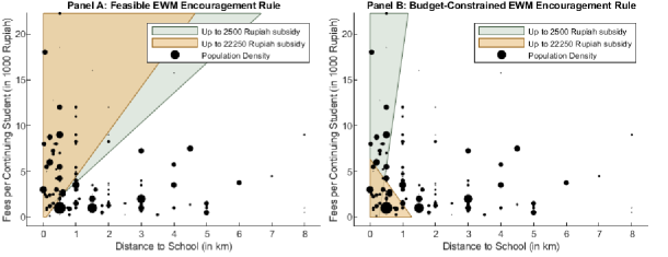
Figure 1: Targeted Subpopulation under Alternative Encouragement Rules

Figure 2 gives a sense of why the subpopulations indicated by the shaded areas in Figure 1 are targeted. It visualizes how the impact of going from the status quo to a full tuition waiver (i.e., $\alpha_{1}=22.25$) differs across individuals with different values of $(Z_{1},Z_{2})$ in terms of treatment take-up and treatment effects. Panel A of Figure 2 displays the level sets of changes in average treatment take-up conditional on $(Z_{1},Z_{2})$, namely the level sets of $(z_{1},z_{2})\mapsto E_{n}[\hat{p}(X,M_{\alpha_{1}}(z))-\hat{p}(X,z)]$. We can see that basically only individuals with low $Z_{2}$ are induced into treatment. Panel B of Figure 2 displays the level sets of average treatment effects for those induced to switch treatment status conditional on $(Z_{1},Z_{2})$, namely the level sets of

$$(z_{1},z_{2})\mapsto\frac{E_{n}\Big{[}\int_{\hat{p}(X,z)}^{\hat{p}(X,M_{\alpha_{1}}(z))}\widehat{\operatorname{MTE}}_{1}(u_{1},X,z_{2})\,du_{1}\Big{]}}{E_{n}[\hat{p}(X,M_{\alpha_{1}}(z))-\hat{p}(X,z)]}.$$

We can see that individuals with low $Z_{1}$ have negative treatment effects for $Z_{2}$ on the left of the zero contour line for changes in treatment take-up. Put together, absent budget constraints, individuals in the upper-left corner are prioritized for the full tuition fee waiver. On the other hand, contour lines where $Z_{1}$ is high are rather steep in both panels, implying that individuals with higher $Z_{1}$ induce higher manipulation costs for the same level of welfare gains. Consequently, the optimal policy under budget constraints trades off welfare gains against costs and gives up individuals with high $Z_{1}$.

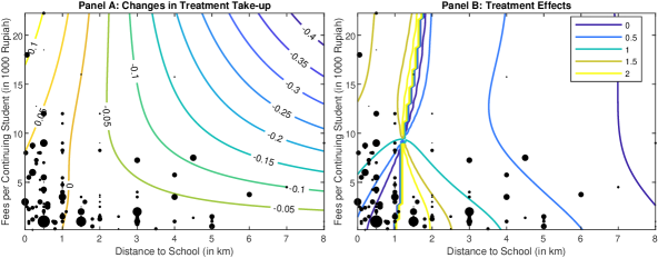
Figure 2: Impact of Going from the Status Quo to a Full Tuition Waiver

Notes: Panel A displays the level sets of changes in treatment take-up. Panel B displays the level sets of treatment effects for those induced to switch treatment status. The size of the black dots indicates the number of individuals with different values of $(Z_{1},Z_{2})$.

6 Conclusion

In this paper, we propose a framework for policy learning that allows for endogenous treatment selection by leveraging a continuous instrumental variable. To deal with failure of unconfoundedness when identifying the social welfare criterion, we incorporate the MTE function. To deal with imperfect compliance when designing policies, we consider encouragement rules in addition to treatment assignment rules. We apply the representation of the social welfare criterion of encouragement rules to the EWM method and derive convergence rates of the worst-case regret. We also consider extensions allowing for multiple instruments and budget constraints. We illustrate the EWM encouragement rule using data from the Indonesian Family Life Survey.

There are several potential extensions and directions for future research. First, our point identification of the social welfare criterion imposes several restrictive parametric assumptions for extrapolations. To relax these assumptions, one might consider incorporating the approach to partial-identifying policy parameters proposed by Mogstad et al. (2018). Second, to improve the convergence rate of the regret, the technique of a doubly robust estimator of the social welfare criterion proposed by Athey and Wager (2021) could be adapted from inverse-propensity weighting to partially linear models.

Appendix Appendix A Proofs

For a binary encouragement rule $G$ described in Section 2.3, define the welfare contrast relative to the baseline policy that allocates everyone to $\alpha_{0}$ and its empirical analogue as

$$\bar{W}(G) =E_{P}\bigg{[}1\{(X,Z)\in G\}\int_{p(X,M_{\alpha_{0}}(Z))}^{p(X,M_{\alpha_{1}}(Z))}\operatorname{MTE}(u,X)\,du\bigg{]}=W(G)-W_{0},$$

$$\bar{W}_{n}(G) =E_{n}\bigg{[}1\{(X,Z)\in G\}\int_{p(X,M_{\alpha_{0}}(Z))}^{p(X,M_{\alpha_{1}}(Z))}\operatorname{MTE}(u,X)\,du\bigg{]}.$$

Appendix A.1 Proof of Theorem 1

Proof.

We have

$$W(\boldsymbol{\alpha}) =E_{P}[Y(1)\cdot D^{\boldsymbol{\alpha}}+Y(0)\cdot(1-D^{\boldsymbol{\alpha}})]$$

$$=E_{P}[Y(1)\cdot 1\{p(X,M_{\boldsymbol{\alpha}(X,Z)}(Z))\geq U\}+Y(0)\cdot 1\{p(X,M_{\boldsymbol{\alpha}(X,Z)}(Z))<U\}]$$

$$=E_{P}[Y(1)\cdot 1\{p(X,Z)\geq U\}+Y(0)\cdot 1\{p(X,Z)<U\}]$$

$$\quad\ +E_{P}[(Y(1)-Y(0))\cdot(1\{p(X,M_{\boldsymbol{\alpha}(X,Z)}(Z))\geq U\}-1\{p(X,Z)\geq U\})]$$

$$=E_{P}[Y]+E_{P}[(Y(1)-Y(0))\cdot(1\{p(X,M_{\boldsymbol{\alpha}(X,Z)}(Z))\geq U\}-1\{p(X,Z)\geq U\})].$$ (A.1)

By the law of iterated expectations, the second term in (A.1) can be written as

$$\quad\ E_{P}[(Y(1)-Y(0))\cdot(1\{p(X,M_{\boldsymbol{\alpha}(X,Z)}(Z))\geq U\}-1\{p(X,Z)\geq U\})]$$

$$=E_{P}[E_{P}[Y(1)-Y(0)|X,Z,U]\cdot(1\{p(X,M_{\boldsymbol{\alpha}(X,Z)}(Z))\geq U\}-1\{p(X,Z)\geq U\})]$$

$$=E_{P}[\operatorname{MTE}(U,X)\cdot(1\{p(X,M_{\boldsymbol{\alpha}(X,Z)}(Z))\geq U\}-1\{p(X,Z)\geq U\})]$$

$$=E_{P}[E_{P}[\operatorname{MTE}(U,X)\cdot(1\{p(X,M_{\boldsymbol{\alpha}(X,Z)}(Z))\geq U\}-1\{p(X,Z)\geq U\})|X,Z]]$$

$$=E_{P}\bigg{[}\int_{0}^{1}\operatorname{MTE}(u,X)\cdot(1\{p(X,M_{\boldsymbol{\alpha}(X,Z)}(Z))\geq u\}-1\{p(X,Z)\geq u\})\,du\bigg{]},$$

where the second equality follows from Assumption 11.2 and the definition of the MTE, and the fourth equality follows from (3). ∎

Appendix A.2 Proof of Corollary 3

Proof.

Define

$$f(X,Z;G)=1\{(X,Z)\in G\}\int_{p(X,M_{\alpha_{0}}(Z))}^{p(X,M_{\alpha_{1}}(Z))}\operatorname{MTE}(u,X)\,du$$

and

$$\mathcal{F}=\{f(\cdot;G):G\in\mathcal{G}\}.$$

By Assumption 22.1, $\mathcal{F}$ is a class of uniformly bounded functions with $\|f\|_{\infty}\leq\bar{M}$ for all $f\in\mathcal{F}$. By Assumption 22.2 and Lemma A.1 of Kitagawa and Tetenov (2018a), $\mathcal{F}$ is a VC-subgraph class of functions with VC-dimension less than or equal to $V$. Then, we can apply Lemma A.4 of Kitagawa and Tetenov (2018a) to obtain

$$E_{P^{n}}\Big{[}\sup_{f\in\mathcal{F}}|E_{n}(f)-E_{P}(f)|\Big{]}\leq C_{1}\bar{M}\sqrt{\frac{V}{n}},$$ (A.2)

where $C_{1}$ is a universal constant. Then, we have

$$\sup_{G\in\mathcal{G}}|\bar{W}_{n}(G)-\bar{W}(G)|=\sup_{f\in\mathcal{F}}|E_{n}(f)-E_{P}(f)|.$$ (A.3)

Following the derivations in Kitagawa and Tetenov (2018b, Eq. (2.2)), we have for any $\tilde{G}\in\mathcal{G}$,

$$W(\tilde{G})-W(\hat{G}_{\mathrm{EWM}}) =\bar{W}(\tilde{G})-\bar{W}_{n}(\hat{G}_{\mathrm{EWM}})+\bar{W}_{n}(\hat{G}_{\mathrm{EWM}})-\bar{W}(\hat{G}_{\mathrm{EWM}})$$

$$\leq\bar{W}(\tilde{G})-\bar{W}_{n}(\tilde{G})+\sup_{G\in\mathcal{G}}|\bar{W}_{n}(G)-\bar{W}(G)|$$

$$\quad\ (\because\bar{W}_{n}(\hat{G}_{\mathrm{EWM}})\geq\bar{W}_{n}(\tilde{G}))$$

$$\leq 2\sup_{G\in\mathcal{G}}|\bar{W}_{n}(G)-\bar{W}(G)|.$$

It follows from (A.2) and (A.3) that

$$\sup_{P\in\mathcal{P}(\bar{M})}E_{P^{n}}\big{[}W_{\mathcal{G}}^{*}-W(\hat{G}_{\mathrm{EWM}})\big{]}\leq 2C_{1}\bar{M}\sqrt{\frac{V}{n}}.$$

∎

Appendix A.3 Proof of Theorem 2

Proof.

We have for any $\tilde{G}\in\mathcal{G}$,

$$\quad\ W(\tilde{G})-W(\hat{G}_{\mathrm{FEWM}})$$

$$\leq\bar{W}(\tilde{G})-\bar{W}_{n}(\tilde{G})+\bar{W}_{n}(\hat{G}_{\mathrm{FEWM}})-\bar{W}(\hat{G}_{\mathrm{FEWM}})$$

$$\quad\ +\bar{W}_{n}(\tilde{G})-\hat{\bar{W}}_{n}(\tilde{G})-\bar{W}_{n}(\hat{G}_{\mathrm{FEWM}})+\hat{\bar{W}}_{n}(\hat{G}_{\mathrm{FEWM}})\quad(\because\hat{\bar{W}}_{n}(\hat{G}_{\mathrm{FEWM}})\geq\hat{\bar{W}}_{n}(\tilde{G}))$$

$$\leq 2\sup_{G\in\mathcal{G}}|\bar{W}_{n}(G)-\bar{W}(G)|+2\sup_{G\in\mathcal{G}}|\bar{W}_{n}(G)-\hat{\bar{W}}_{n}(G)|,$$

where $\hat{\bar{W}}_{n}(G)$ is defined as in (11). In view of (A.2) and (A.3), it suffices to show that

$$\limsup_{n\to\infty}\sup_{P\in\mathcal{P}_{p}\cap\mathcal{P}_{\mathrm{MTE}}}(\phi_{n}\wedge\psi_{n})E_{P^{n}}\Big{[}\sup_{G\in\mathcal{G}}|\bar{W}_{n}(G)-\hat{\bar{W}}_{n}(G)|\Big{]}<\infty.$$ (A.4)

By the triangle inequality and Assumption 33.1,

$$\sup_{G\in\mathcal{G}}|\bar{W}_{n}(G)-\hat{\bar{W}}_{n}(G)| \leq E_{n}\bigg{[}\bigg{|}\int_{\hat{p}(X,M_{\alpha_{0}}(Z))}^{\hat{p}(X,M_{\alpha_{1}}(Z))}\widehat{\operatorname{MTE}}(u,X)\,du-\int_{p(X,M_{\alpha_{0}}(Z))}^{p(X,M_{\alpha_{1}}(Z))}\operatorname{MTE}(u,X)\,du\bigg{|}\bigg{]}$$

$$\leq E_{n}\bigg{[}\bigg{|}\int_{\hat{p}(X,M_{\alpha_{0}}(Z))}^{\hat{p}(X,M_{\alpha_{1}}(Z))}(\widehat{\operatorname{MTE}}(u,X)-\operatorname{MTE}(u,X))\,du\bigg{|}\bigg{]}$$

$$\quad\ +E_{n}\bigg{[}\bigg{|}\int_{p(X,M_{\alpha_{1}}(Z))}^{\hat{p}(X,M_{\alpha_{1}}(Z))}\operatorname{MTE}(u,X)\,du\bigg{|}\bigg{]}+E_{n}\bigg{[}\bigg{|}\int_{p(X,M_{\alpha_{0}}(Z))}^{\hat{p}(X,M_{\alpha_{0}}(Z))}\operatorname{MTE}(u,X)\,du\bigg{|}\bigg{]}$$

$$\leq E_{n}\bigg{[}\bigg{|}\int_{0}^{1}(\widehat{\operatorname{MTE}}(u,X)-\operatorname{MTE}(u,X))\,du\bigg{|}\bigg{]}$$

$$\quad\ +E_{n}\bigg{[}\bigg{|}\int_{p(X,M_{\alpha_{1}}(Z))}^{\hat{p}(X,M_{\alpha_{1}}(Z))}\operatorname{MTE}(u,X)\,du\bigg{|}\bigg{]}+E_{n}\bigg{[}\bigg{|}\int_{p(X,M_{\alpha_{0}}(Z))}^{\hat{p}(X,M_{\alpha_{0}}(Z))}\operatorname{MTE}(u,X)\,du\bigg{|}\bigg{]}.$$

For $\tilde{Z}\in\{M_{\alpha_{0}}(Z),M_{\alpha_{1}}(Z)\}$,

$$E_{n}\bigg{[}\bigg{|}\int_{p(X,\tilde{Z})}^{\hat{p}(X,\tilde{Z})}\operatorname{MTE}(u,X)\,du\bigg{|}\bigg{]} \leq E_{n}\bigg{[}\int_{p(X,\tilde{Z})}^{\hat{p}(X,\tilde{Z})}|\operatorname{MTE}(u,X)|\,du\bigg{]}$$

$$\leq E_{n}\bigg{[}C(X)|\hat{p}(X,\tilde{Z})-p(X,\tilde{Z})|\bigg{]}$$

$$\leq E_{n}[C(X)]\sup_{(x,z)\in\mathcal{X}\times\bar{\mathcal{Z}}}|\hat{p}(x,z)-p(x,z)|$$

$$\leq(E_{n}-E_{P})[C(X)]\sup_{(x,z)\in\mathcal{X}\times\bar{\mathcal{Z}}}|\hat{p}(x,z)-p(x,z)|$$

$$\quad\ +E_{P}[C(X)]\sup_{(x,z)\in\mathcal{X}\times\bar{\mathcal{Z}}}|\hat{p}(x,z)-p(x,z)|,$$

where the second inequality follows from Assumption 44.1. By Assumption 44.2,

$$\limsup_{n\to\infty}\sup_{P\in\mathcal{P}_{\mathrm{MTE}}}n^{1/2}E_{P^{n}}[(E_{n}-E_{P})[C(X)]]<\infty.$$

Combining the above, by Assumptions 33.2, 44.2 and 44.3, (A.4) holds. ∎

Appendix A.4 Proof of Theorem 3

Proof.

For any $\epsilon>0$,

$$\Pr\textsubscript{$\!P^{n}$}\{W(G^{*}_{P})-W(\hat{G}_{\mathrm{BEWM}})>\epsilon\} =\Pr\textsubscript{$\!P^{n}$}\{\bar{W}(G^{*}_{P})-\bar{W}(\hat{G}_{\mathrm{BEWM}})>\epsilon,\hat{B}_{n}(G^{*}_{P})\leq\kappa\}$$

$$\quad\ +\Pr\textsubscript{$\!P^{n}$}\{\bar{W}(G^{*}_{P})-\bar{W}(\hat{G}_{\mathrm{BEWM}})>\epsilon,\hat{B}_{n}(G^{*}_{P})>\kappa\}$$

$$=P_{1}+P_{2}.$$

Noting that $\hat{B}_{n}(G^{*}_{P})\leq\kappa$ implies $\hat{\bar{W}}_{n}(\hat{G}_{\mathrm{BEWM}})\geq\hat{\bar{W}}_{n}(G^{*}_{P})$,

$$P_{1} \leq\Pr\textsubscript{$\!P^{n}$}\{\bar{W}(G^{*}_{P})-\hat{\bar{W}}_{n}(G^{*}_{P})+\hat{\bar{W}}_{n}(\hat{G}_{\mathrm{BEWM}})-\bar{W}(\hat{G}_{\mathrm{BEWM}})>\epsilon,\hat{B}_{n}(G^{*}_{P})\leq\kappa\}$$

$$\leq\Pr\textsubscript{$\!P^{n}$}\Big{\{}2\sup_{G\in\mathcal{G}}|\bar{W}(G)-\hat{\bar{W}}_{n}(G)|>\epsilon\Big{\}}.$$

On the other hand, $B(G^{*}_{P})\leq\kappa$, and thus

$$P_{2}\leq\Pr\textsubscript{$\!P^{n}$}\{\hat{B}_{n}(G^{*}_{P})>\kappa\}\leq\Pr\textsubscript{$\!P^{n}$}\{\hat{B}_{n}(G^{*}_{P})>B(G^{*}_{P})\}.$$

Combining the above, we have

$$\quad\ \Pr\textsubscript{$\!P^{n}$}\{W(G^{*}_{P})-W(\hat{G}_{\mathrm{BEWM}})>\epsilon\}$$

$$\leq\Pr\textsubscript{$\!P^{n}$}\Big{\{}\sup_{G\in\mathcal{G}}|\bar{W}(G)-\hat{\bar{W}}_{n}(G)|>\epsilon\Big{\}}+\Pr\textsubscript{$\!P^{n}$}\{\hat{B}_{n}(G^{*}_{P})>B(G^{*}_{P})\}$$

$$\leq\Pr\textsubscript{$\!P^{n}$}\Big{\{}\sup_{G\in\mathcal{G}}|\bar{W}(G)-\hat{\bar{W}}_{n}(G)|>\epsilon\Big{\}}+\sup_{\epsilon^{\prime}>0}\Pr\textsubscript{$\!P^{n}$}\{\hat{B}_{n}(G^{*}_{P})-B(G^{*}_{P})>\epsilon^{\prime}\}$$

$$\leq\Pr\textsubscript{$\!P^{n}$}\Big{\{}\sup_{G\in\mathcal{G}}|\bar{W}(G)-\hat{\bar{W}}_{n}(G)|>\epsilon\Big{\}}+\sup_{\epsilon^{\prime}>0}\Pr\textsubscript{$\!P^{n}$}\Big{\{}\sup_{G\in\mathcal{G}}|B(G)-\hat{B}_{n}(G)|>\epsilon^{\prime}\Big{\}}.$$ (A.5)

Also, for any $\epsilon>0$,

$$\Pr\textsubscript{$\!P^{n}$}\{B(\hat{G}_{\mathrm{BEWM}})-\kappa>\epsilon\} \leq\Pr\textsubscript{$\!P^{n}$}\{B(\hat{G}_{\mathrm{BEWM}})-\hat{B}_{n}(\hat{G}_{\mathrm{BEWM}})>\epsilon\}\quad(\because\hat{B}_{n}(\hat{G}_{\mathrm{BEWM}})\leq\kappa)$$

$$\leq\Pr\textsubscript{$\!P^{n}$}\Big{\{}\sup_{G\in\mathcal{G}}|B(G)-\hat{B}_{n}(G)|>\epsilon\Big{\}}.$$ (A.6)

Define

$$B_{n}(G)=E_{n}[ 1\{(X,Z)\in G\}\cdot|M_{\alpha_{1}}(Z)-Z|\cdot p(X,M_{\alpha_{1}}(Z))$$

$$+1\{(X,Z)\notin G\}\cdot|M_{\alpha_{0}}(Z)-Z|\cdot p(X,M_{\alpha_{0}}(Z))].$$

By the triangle inequality, for any $G\in\mathcal{G}$,

$$|\bar{W}(G)-\hat{\bar{W}}_{n}(G)| \leq|\bar{W}(G)-\bar{W}_{n}(G)|+|\bar{W}_{n}(G)-\hat{\bar{W}}_{n}(G)|,$$ (A.7)

$$|B(G)-\hat{B}_{n}(G)| \leq|B(G)-B_{n}(G)|+|B_{n}(G)-\hat{B}_{n}(G)|.$$ (A.8)

From the same argument as the proof of (A.3), we can apply Lemma A.4 of Kitagawa and Tetenov (2018a) to obtain

$$\sup_{P\in\mathcal{P}^{\prime}(\bar{M})}E_{P^{n}}\Big{[}\sup_{G\in\mathcal{G}}|\bar{W}_{n}(G)-\bar{W}(G)|\Big{]} \leq O(n^{-1/2}),$$ (A.9)

$$\sup_{P\in\mathcal{P}^{\prime}(\bar{M})}E_{P^{n}}\Big{[}\sup_{G\in\mathcal{G}}|B_{n}(G)-B(G)|\Big{]} \leq O(n^{-1/2}).$$ (A.10)

On the other hand, note that

$$\sup_{G\in\mathcal{G}}|B_{n}(G)-\hat{B}_{n}(G)|\leq E_{n}[ C_{\alpha_{1}}(X,Z)\cdot|\hat{p}(X,M_{\alpha_{1}}(Z))-p(X,M_{\alpha_{1}}(Z))|$$

$$+C_{\alpha_{0}}(X,Z)\cdot|\hat{p}(X,M_{\alpha_{0}}(Z))-p(X,M_{\alpha_{0}}(Z))|]$$

$$\leq 2\bar{M} \sup_{(x,z)\in\mathcal{X}\times\bar{\mathcal{Z}}}|\hat{p}(x,z)-p(x,z)|,$$

where the second inequality follows from Assumption 55.1. Hence, by (5),

$$\limsup_{n\to\infty}\sup_{P\in\mathcal{P}_{p}}\psi_{n}E_{P^{n}}\Big{[}\sup_{G\in\mathcal{G}}|B_{n}(G)-\hat{B}_{n}(G)|\Big{]}<\infty.$$ (A.11)

By Markov’s inequality and (A.4)–(A.11), we have that, for any $\epsilon>0$,

$$\lim_{n\to\infty}\sup_{P\in\mathcal{P}^{\prime}(\bar{M})\cap\mathcal{P}_{p}\cap\mathcal{P}_{\mathrm{MTE}}}\Pr\textsubscript{$\!P^{n}$}\{W(\hat{G}_{\mathrm{BEWM}})-W(G^{*}_{P})<-\epsilon\}=0,$$

$$\lim_{n\to\infty}\sup_{P\in\mathcal{P}^{\prime}(\bar{M})\cap\mathcal{P}_{p}\cap\mathcal{P}_{\mathrm{MTE}}}\Pr\textsubscript{$\!P^{n}$}\{B(\hat{G}_{\mathrm{BEWM}})-\kappa>\epsilon\}=0.$$

∎

Appendix Appendix B Encouragement Rules with a Binary Instrument

In many applications, the instrument is binary by construction. For completeness, we present a discussion of cases in which a binary instrument is intervened upon. An encouragement rule is a mapping from $\mathcal{X}$ to $\{0,1\}$ and can be indexed by its decision set $G\subset\mathcal{X}$ such that the policymaker assigns individuals with $X\in G$ to encouragement $Z=1$. For example, the encouragement could be eligibility for welfare programs such as the National Job Training Partnership Act (JTPA) or the 401(k) retirement program.

Under (1), (3), and Assumption 1, the treatment choice under encouragement rule $G$ is given by

$$D^{G}=1\{p(X,1)\geq U\}\cdot 1\{X\in G\}+1\{p(X,0)\geq U\}\cdot 1\{X\notin G\}.$$

We can represent the social welfare criterion as a function of the MTE:

$$W(G) =E_{P}[Y(1)\cdot D^{G}+Y(0)\cdot(1-D^{G})]$$

$$=W_{0}+E_{P}\bigg{[}1\{X\in G\}\int_{p(X,0)}^{p(X,1)}\operatorname{MTE}(u,X)\,du\bigg{]},$$

where $W_{0}=E_{P}[Y(1)\cdot 1\{p(X,0)\geq U\}+Y(0)\cdot 1\{p(X,0)<U\}]$ does not depend on $G$. If we further impose

1. (IV positivity) $0<\Pr_{P}(Z=1|X)<1$ almost surely,

we can then derive a more convenient representation of the social welfare criterion:

$$W(G)=E_{P}[ (Y(1)\cdot 1\{p(X,1)\geq U\}+Y(0)\cdot 1\{p(X,1)<U\})\cdot 1\{X\in G\}$$

$$+(Y(1)\cdot 1\{p(X,0)\geq U\}+Y(0)\cdot 1\{p(X,0)<U\})\cdot 1\{X\notin G\}]$$

$$=E_{P}[ E_{P}[Y|X,Z=1]\cdot 1\{X\in G\}+E_{P}[Y|X,Z=0]\cdot 1\{X\notin G\}]$$

$$=E_{P}\bigg{[} \frac{YZ}{q(X)}\cdot 1\{X\in G\}+\frac{Y(1-Z)}{1-q(X)}\cdot 1\{X\notin G\}\bigg{]},$$

where $q(X)=E_{P}[Z|X]$. Given a feasible class $\mathcal{G}\subset\{G\subset\mathcal{X}\}$ of encouragement rules, the optimal encouragement rule, if $P$ is known, is $G^{*}_{P}\in\operatorname*{arg\,max}_{G\in\mathcal{G}}W(G)$. The optimal encouragement rule is identified without observing the treatment variable $D$. Intuitively, the optimization problem amounts to finding the optimal treatment rule that assigns $Z$ rather than $D$, from an intention-to-treat perspective. In this case, Assumption 1(i) warrants unconfoundedness, and the analysis essentially follows the original EWM framework. It is worth noting that $W(G)$ only measures the indirect effect of treatment via the impact of encouragement upon eventual treatment receipt. For always-takers and never-takers, no encouragement rule can possibly alter their outcomes.

We proceed to present two extensions analogous to those in Section 4. In Appendix B.1, we allow for multiple instruments. In Appendix B.2, we incorporate a budget constraint.

Appendix B.1 Multiple Instruments

Consider a setting in which there are $L$ instruments available. Let $Z_{1}$ be the binary instrument that can be manipulated, $Z_{-1}\equiv(Z_{2},\dots,Z_{L})^{\prime}\in\mathcal{Z}_{-1}\subset\mathbb{R}^{L-1}$ be a vector of additional instruments, and $Z=(Z_{1},Z_{-1}^{\prime})^{\prime}$. The policymaker can choose an encouragement rule based on $(X,Z_{-1})$, and the set of encouragement rules is indexed by $G\subset\mathcal{X}\times\mathcal{Z}_{-1}$. Under (1), (9), Assumption 1’, and $0<\Pr_{P}(Z=1|X,Z_{-1})<1$ almost surely, the social welfare criterion is given by

$$W(G)=E_{P}\bigg{[}\frac{YZ_{1}}{q(X,Z_{-1})}\cdot 1\{(X,Z_{-1})\in G\}+\frac{Y(1-Z_{1})}{1-q(X,Z_{-1})}\cdot 1\{(X,Z_{-1})\notin G\}\bigg{]},$$

where $q(X,Z_{-1})=E_{P}[Z_{1}|X,Z_{-1}]$. The additional instruments $Z_{-1}$ are treated equivalently to covariates $X$. With further assumptions imposed on the selection behavior, we can produce an interpretation of which subpopulation benefits from the encouragement rule. In particular, we assume

1. (Component-wise monotonic propensity score) For each $x\in\mathcal{X}$, $z\mapsto p(x,z)$ is component-wise monotonic in $z$.

In the case of two binary instruments, under (9) and Assumptions 1’ and B.2 with the direction of component-wise monotonicity normalized to be increasing, we can partition the population into the six well-defined compliance groups presented in Table B.1.

Table B.1: Compliance Groups (Mogstad et al., 2021, Proposition 4)

Name	$D(0,0)$	$D(0,1)$	$D(1,0)$	$D(1,1)$
Never-takers (nt)	N	N	N	N
Always-takers (at)	T	T	T	T
$Z_{1}$ compliers (1c)	N	N	T	T
$Z_{2}$ compliers (2c)	N	T	N	T
Eager compliers (ec)	N	T	T	T
Reluctant compliers (rc)	N	N	N	T

• Notes: “T” indicates treatment, and “N” indicates non-treatment.

The social welfare criterion can be written as

$$W(G) =E_{P}[Y(D(0,Z_{2})]+E_{P}[(Y(1)-Y(0))(D(1,Z_{2})-D(0,Z_{2}))\cdot 1\{(X,Z_{2})\in G\}]$$

$$=E_{P}[Y(D(0,Z_{2})]+E_{P}[E_{P}[(Y(1)-Y(0))(D(1,1)-D(0,1))|X]\Pr\!\textsubscript{$P$}(Z_{2}=1|X)\cdot 1\{(X,1)\in G\}]$$

$$\quad\ +E_{P}[E_{P}[(Y(1)-Y(0))(D(1,0)-D(0,0))|X]\Pr\!\textsubscript{$P$}(Z_{2}=0|X)\cdot 1\{(X,0)\in G\}].$$

Denote by $H\in\mathcal{H}=\{\text{nt},\text{at},\text{1c},\text{2c},\text{ec},\text{rc}\}$ the compliance group identity. For each $h\in\mathcal{H}$, let $\pi_{h}(X)=\Pr_{P}(H=h|X)$ be the conditional population share of compliance group $h$ and $\Delta_{h}(X)=E_{P}[Y(1)-Y(0)|X,H=h]$ be the compliance-group-specific CATE. Then,

$$E_{P}[(Y(1)-Y(0))(D(1,1)-D(0,1))|X]=\pi_{\mathrm{1c}}(X)\Delta_{\mathrm{1c}}(X)+\pi_{\mathrm{rc}}(X)\Delta_{\mathrm{rc}}(X),$$

$$E_{P}[(Y(1)-Y(0))(D(1,0)-D(0,0))|X]=\pi_{\mathrm{1c}}(X)\Delta_{\mathrm{1c}}(X)+\pi_{\mathrm{ec}}(X)\Delta_{\mathrm{ec}}(X).$$

Therefore, besides $Z_{1}$ compliers, the encouragement rule would affect the outcomes of reluctant compliers with $Z_{2}=1$ and the outcomes of eager compliers with $Z_{2}=0$.

Appendix B.2 Budget Constraints

The causal mechanism that $Z$ affects $Y$ through $D$ will play a role if we impose a resource constraint. Suppose that the proportion of the population that could receive treatment cannot exceed $\kappa\in(0,1)$. Then we face a constrained optimization problem:

$$\max_{G\in\mathcal{G}}W(G)\text{ s.t. }E_{P}[1\{p(X,1)\geq U\}\cdot 1\{X\in G\}]\leq\kappa.$$ (B.1)

One simple idea is to enforce random rationing, as considered by Kitagawa and Tetenov (2018b). Assume that, if $G$ violates the resource constraint, then the encouragement is randomly allocated to a fraction $\frac{\kappa}{E_{P}[1\{p(X,1)\geq U\}\cdot 1\{X\in G\}]}$ of the assigned recipients with $X\in G$ independently of $(X,Y(1),Y(0))$. Under (1), (3), and Assumptions 1 and B.1, we can define the resource-constrained welfare criterion as

$$W^{\kappa}(G)=W_{0}+E_{P}\bigg{[}\bigg{(}\frac{YZ}{q(X)}-\frac{Y(1-Z)}{1-q(X)}\bigg{)}\cdot 1\{X\in G\}\bigg{]}\min\bigg{\{}1,\frac{\kappa}{E_{P}\big{[}\frac{DZ}{q(X)}\cdot 1\{X\in G\}\big{]}}\bigg{\}}.$$

The optimal encouragement rule under random rationing is then $G^{*,\kappa}_{P}\in\operatorname*{arg\,max}_{G\in\mathcal{G}}W^{\kappa}(G)$.

When $\mathcal{G}$ is unrestricted, (B.1) coincides with the constrained optimization problem studied by Qiu et al. (2021). They note that this corresponds to a fractional knapsack problem and has a closed-form solution, which assigns encouragement to recipients with $X\in G$ in decreasing order of benefit-cost ratio $[\frac{YZ}{q(X)}-\frac{Y(1-Z)}{1-q(X)}]/\frac{DZ}{q(X)}$ until the resources are exhausted. The resulting encouragement rule uses the limited resources more efficiently than $G^{*,\kappa}_{P}$. If restrictions are placed on $\mathcal{G}$, there may be no closed-form solution to (B.1).

Appendix Appendix C Sup-norm Convergence Rate in Expectation for Series Estimators

Let us introduce some notations. Let $\lambda_{\mathrm{min}}(\cdot)$ and $\lambda_{\mathrm{max}}(\cdot)$ denote the smallest and largest eigenvalues, respectively, of a matrix. The exponent ^- denotes the Moore–Penrose generalized inverse. $\|\cdot\|$ denotes the Euclidean norm when applied to vectors and the matrix spectral norm (i.e., the largest singular value) when applied to matrices. If $\{a_{n}:n\geq 1\}$ and $\{b_{n}:n\geq 1\}$ are two sequences of nonnegative numbers, $a_{n}\lesssim b_{n}$ means that there exists a finite positive $C$ such that $a_{n}\leq Cb_{n}$ for all sufficiently large $n$. Let $L^{\infty}(X)$ denote the space of bounded functions under the sup norm, i.e., if $f:\mathcal{X}\to\mathbb{R}$ then $\|f\|_{\infty}=\sup_{x\in\mathcal{X}}|f(x)|$.

We consider the nonparametric regression model

$$Y=h_{0}(X)+\epsilon,\quad E_{P}[\epsilon|X]=0,$$

where $Y\in\mathbb{R}$ and $X\in\mathcal{X}\subset\mathbb{R}^{d_{x}}$. Let $\{(Y_{i},X_{i})\}_{i=1}^{n}$ be a random sample. We consider the standard series least-squares estimator of $h_{0}$:

$$\hat{h}(x)=b^{K}(x)^{\prime}(B^{\prime}B)^{-}B^{\prime}\mathbf{Y},$$

where $b_{K1},\dots,b_{KK}$ are a collection of $K$ sieve basis functions, and

$$b^{K}(x)=(b_{K1}(x),\dots,b_{KK}(x))^{\prime},\quad B=(b^{K}(X_{1}),\dots,b^{K}(X_{n}))^{\prime},\quad\mathbf{Y}=(Y_{1},\dots,Y_{n})^{\prime}.$$

We may further impose certain types of restrictions to avoid the curse of dimensionality. For example, we could use a series estimator based on a partially linear additive regression model defined in Carneiro and Lee (2009, Eq. (4.1)).

Define $\zeta_{K}=\sup_{x}\|b^{K}(x)\|$ and $\lambda_{K}=[\lambda_{\mathrm{min}}(E_{P}[b^{K}(X_{i})b^{K}(X_{i})^{\prime}])]^{-1/2}$. We introduce some regularity conditions that are standard in the literature on series estimation.

1. $\mathcal{X}$ is a Cartesian product of compact connected intervals on which $X$ has a probability density function that is bounded away from zero.

2. $\lambda_{\mathrm{min}}(E_{P}[b^{K}(X_{i})b^{K}(X_{i})^{\prime}])>0$ for each $K$.

3. There exist $\sigma,\tilde{c}>0$ such that $\sup_{x}E_{P}[|\epsilon_{i}|^{q}|X_{i}=x]\leq\frac{q!}{2}\sigma^{2}\tilde{c}^{q-2}$ for all $q\geq 2$.

4. $\inf_{h\in B_{K}}\|h_{0}-h\|_{\infty}\lesssim K^{-\alpha}$ as $K\to\infty$.

Let $\tilde{b}^{K}(x)$ denote the orthonormalized vector of basis functions, namely

$$\tilde{b}^{K}(x)=E_{P}[b^{K}(X_{i})b^{K}(X_{i})^{\prime}]^{-1/2}b^{K}(x)$$

and let $\tilde{B}=(\tilde{b}^{K}(X_{1}),\dots,\tilde{b}^{K}(X_{n}))^{\prime}$. The following lemma gives an exponential tail bound for $\|\tilde{B}^{\prime}\tilde{B}/n-I_{k}\|$.

Lemma C.1.

Under Assumption C.2,

$$\Pr\textsubscript{\!$P^{n}$}\Big{(}\|\tilde{B}^{\prime}\tilde{B}/n-I_{k}\|\geq\frac{1}{2}\Big{)}\leq 2K\exp\Big{(}\frac{-C_{1}n}{\zeta_{K}^{2}\lambda_{K}^{2}+1}\Big{)}$$

for some finite positive constant $C_{1}$.

Proof.

Follows from Theorem 4.1 of Chen and Christensen (2015) by setting $\Xi_{i}=n^{-1}(\tilde{b}^{K}(X_{i})\tilde{b}^{K}(X_{i})^{\prime}-I_{K})$ and noting that $\max_{1\leq i\leq n}\|\Xi_{i}\|\leq n^{-1}(\zeta_{K}^{2}\lambda_{K}^{2}+1)$ and $\max\{\|\sum_{i=1}^{n}E_{P}[\Xi_{i}\Xi_{i}^{\prime}]\|,\|\sum_{i=1}^{n}E_{P}[\Xi_{i}^{\prime}\Xi_{i}]\|\}\leq n^{-1}(\zeta_{K}^{2}\lambda_{K}^{2}+1)$. ∎

Let $B_{K}=\operatorname{clsp}\{b_{K1},\dots,b_{KK}\}$ be a general linear sieve space. Let $\tilde{h}$ denote the projection of $h_{0}$ onto $B_{K}$ under the empirical measure, that is,

$$\tilde{h}(x)=b^{K}(x)^{\prime}(B^{\prime}B)^{-}B^{\prime}H_{0}=\tilde{b}^{K}(x)^{\prime}(\tilde{B}^{\prime}\tilde{B})^{-}\tilde{B}^{\prime}H_{0},$$

where $H_{0}=(h_{0}(X_{1}),\dots,h_{0}(X_{n}))^{\prime}$. We can bound the sup-norm distance $\|\hat{h}-h_{0}\|_{\infty}$ using

$$\|\hat{h}-h_{0}\|_{\infty} \leq\|h_{0}-\tilde{h}\|_{\infty}+\|\hat{h}-\tilde{h}\|_{\infty}$$

$$=\text{bias term}+\text{variance term}.$$

The following lemma provides an exponential tail bound on the sup-norm variance term.

Lemma C.2.

Let $\mathcal{A}_{n}$ denote the event on which $\|\tilde{B}^{\prime}\tilde{B}/n-I_{k}\|\leq\frac{1}{2}$. Under Assumptions C.1–C.3, for any $\delta>0$,

$$\Pr\textsubscript{\!$P^{n}$}\big{(}\big{\{}\|\hat{h}-\tilde{h}\|_{\infty}\geq\delta\big{\}}\cap\mathcal{A}_{n}\big{)}\lesssim\exp\Big{\{}-\frac{C_{2}n\delta^{2}}{\zeta_{K}^{2}\lambda_{K}^{2}}\Big{\}}$$

for some finite positive constant $C_{2}$.

Proof.

By rotational invariance, we have

$$\hat{h}(x)-\tilde{h}(x)=\tilde{b}^{K}(x)^{\prime}(\tilde{B}^{\prime}\tilde{B}/n)^{-}\tilde{B}^{\prime}e/n,$$

where $e=(\epsilon_{1},\dots,\epsilon_{n})^{\prime}$. Define $G_{i,n}(x)=\tilde{b}^{K}(x)^{\prime}(\tilde{B}^{\prime}\tilde{B}/n)^{-}\tilde{b}^{K}(X_{i})1_{\mathcal{A}_{n}}$ where $1_{\mathcal{A}_{n}}$ denotes the indicator function of $\mathcal{A}_{n}$. Then $(\hat{h}(x)-\tilde{h}(x))1_{\mathcal{A}_{n}}=\frac{1}{n}\sum_{i=1}^{n}G_{i,n}(x)\epsilon_{i}$. Note that $\|(\tilde{B}^{\prime}\tilde{B}/n)^{-1}\|\leq 2$ on $\mathcal{A}_{n}$. Then, for $q\geq 2$,

$$\quad\sum_{i=1}^{n}E_{P^{n}}[(n^{-1}G_{i,n}(x))^{2}|\epsilon_{i}|^{q}|X_{1}^{n}]$$

$$=\frac{1}{n^{2}}\sum_{i=1}^{n}E_{P}[|\epsilon_{i}|^{q}|X_{i}]\tilde{b}^{K}(x)^{\prime}(\tilde{B}^{\prime}\tilde{B}/n)^{-}\tilde{b}^{K}(X_{i})\tilde{b}^{K}(X_{i})^{\prime}1_{\mathcal{A}_{n}}(\tilde{B}^{\prime}\tilde{B}/n)^{-}\tilde{b}^{K}(x)$$

$$\leq\sup_{x}E_{P}[|\epsilon_{i}|^{q}|X_{i}=x]\frac{1}{n^{2}}\sum_{i=1}^{n}\tilde{b}^{K}(x)^{\prime}(\tilde{B}^{\prime}\tilde{B}/n)^{-}\tilde{b}^{K}(X_{i})\tilde{b}^{K}(X_{i})^{\prime}1_{\mathcal{A}_{n}}(\tilde{B}^{\prime}\tilde{B}/n)^{-}\tilde{b}^{K}(x)$$

$$\leq\frac{q!}{2}\sigma^{2}\tilde{c}^{q-2}\frac{1}{n}\tilde{b}^{K}(x)^{\prime}(\tilde{B}^{\prime}\tilde{B}/n)^{-}(\tilde{B}^{\prime}\tilde{B}/n)1_{\mathcal{A}_{n}}(\tilde{B}^{\prime}\tilde{B}/n)^{-}\tilde{b}^{K}(x)$$

$$\leq\frac{q!}{2}\sigma^{2}\tilde{c}^{q-2}\frac{2\zeta_{K}^{2}\lambda_{K}^{2}}{n}.$$

Moreover, for $q\geq 3$,

$$\quad\sum_{i=1}^{n}E_{P^{n}}[|n^{-1}G_{i,n}(x)\epsilon_{i}|^{q}|X_{1}^{n}]$$

$$\leq n^{-(q-2)}\sup_{x}|\tilde{b}^{K}(x)^{\prime}(\tilde{B}^{\prime}\tilde{B}/n)^{-}1_{\mathcal{A}_{n}}\tilde{b}^{K}(x)|^{q-2}\sum_{i=1}^{n}E_{P^{n}}[(n^{-1}G_{i,n}(x))^{2}|\epsilon_{i}|^{q}|X_{1}^{n}]$$

$$\leq\Big{(}\frac{2\zeta_{K}^{2}\lambda_{K}^{2}}{n}\Big{)}^{q-2}\frac{q!}{2}\sigma^{2}\tilde{c}^{q-2}\frac{2\zeta_{K}^{2}\lambda_{K}^{2}}{n}$$

$$=\frac{q!}{2}\sigma^{2}\frac{2\zeta_{K}^{2}\lambda_{K}^{2}}{n}\Big{(}\tilde{c}\frac{2\zeta_{K}^{2}\lambda_{K}^{2}}{n}\Big{)}^{q-2}.$$

Hence, the conditions of Theorem 2.10 of Boucheron et al. (2013) hold with $v=\sigma^{2}\frac{2\zeta_{K}^{2}\lambda_{K}^{2}}{n}$ and $c=\tilde{c}\frac{2\zeta_{K}^{2}\lambda_{K}^{2}}{n}$. By their Corollary 2.11, we have

$$\quad\Pr\textsubscript{\!$P^{n}$}\big{(}\big{\{}\|\hat{h}-\tilde{h}\|_{\infty}\geq\delta\big{\}}\cap\mathcal{A}_{n}\big{)}$$

$$=\Pr\textsubscript{\!$P^{n}$}\Big{(}\Big{\{}\sup_{x}\Big{|}\frac{1}{n}\sum_{i=1}^{n}G_{i,n}(x)\epsilon_{i}\Big{|}\geq\delta\Big{\}}\cap\mathcal{A}_{n}\Big{)}$$

$$\lesssim\exp\Big{\{}-\frac{C_{2}n\delta^{2}}{\zeta_{K}^{2}\lambda_{K}^{2}}\Big{\}}$$

for some finite positive constant $C_{2}$. ∎

Let $P_{K,n}$ be the empirical projection operator onto $B_{K}$, namely

$$P_{K,n}h(x)=b^{K}(x)^{\prime}(B^{\prime}B)^{-}B^{\prime}H=\tilde{b}^{K}(x)^{\prime}(\tilde{B}^{\prime}\tilde{B})^{-}\tilde{B}^{\prime}H=\tilde{h}(x)$$

where $H=(h(X_{1}),\dots,h(X_{n}))^{\prime}$. Let

$$\|P_{K,n}\|_{\infty}=\sup_{h\in L^{\infty}(X):\|h\|_{\infty}\neq 0}\frac{\|P_{K,n}h\|_{\infty}}{\|h\|_{\infty}}$$

denote the sup operator norm of $P_{K,n}$. The following lemma provides a bound on the sup-norm bias term.

Lemma C.3.

Under Assumptions C.1 and C.2,

$$\|\tilde{h}-h_{0}\|_{\infty}\leq(1+\|P_{K,n}\|_{\infty})\inf_{h\in B_{K}}\|h_{0}-h\|_{\infty}.$$

and $\|1_{\mathcal{A}_{n}}P_{K,n}\|_{\infty}\leq\sqrt{2}\zeta_{K}\lambda_{K}$.

Proof.

First, for any $h\in B_{K}$,

$$\|\tilde{h}-h_{0}\|_{\infty} =\|\tilde{h}-h+h-h_{0}\|_{\infty}$$

$$=\|P_{K,n}(h_{0}-h)+h-h_{0}\|_{\infty}$$

$$\leq\|P_{K,n}(h_{0}-h)\|_{\infty}+\|h-h_{0}\|_{\infty}$$

$$\leq(1+\|P_{K,n}\|_{\infty})\|h-h_{0}\|_{\infty}.$$

Taking the infimum over $h\in B_{K}$ yields the first result. Second, take any $h\in L^{\infty}(X)$ with $\|h\|_{\infty}\neq 0$. By the Cauchy–Schwarz inequality, we have

$$|1_{\mathcal{A}_{n}}P_{K,n}h(x)| \leq\|\tilde{b}^{K}(x)\|\|1_{\mathcal{A}_{n}}(\tilde{B}^{\prime}\tilde{B}/n)^{-}\tilde{B}^{\prime}H/n\|$$

$$\leq\zeta_{K}\lambda_{K}\|1_{\mathcal{A}_{n}}(\tilde{B}^{\prime}\tilde{B}/n)^{-}\tilde{B}^{\prime}H/n\|$$

uniformly over $x$. On $\mathcal{A}_{n}$, $\|\tilde{B}^{\prime}\tilde{B}/n-I_{k}\|\leq\frac{1}{2}$ and thus $\lambda_{\mathrm{min}}(\tilde{B}^{\prime}\tilde{B}/n)\geq\frac{1}{2}$. Then,

$$\|1_{\mathcal{A}_{n}}(\tilde{B}^{\prime}\tilde{B}/n)^{-}\tilde{B}^{\prime}H/n\|^{2} =1_{\mathcal{A}_{n}}(H^{\prime}\tilde{B}/n(\tilde{B}^{\prime}\tilde{B}/n)^{-1}(\tilde{B}^{\prime}\tilde{B}/n)^{-1}\tilde{B}^{\prime}H/n$$

$$\leq 2(H^{\prime}\tilde{B}/n(\tilde{B}^{\prime}\tilde{B}/n)^{-1}\tilde{B}^{\prime}H/n$$

$$\leq 2\|h\|^{2}\leq 2\|h\|_{\infty}^{2},$$

where the second-last inequality follows from $1_{\mathcal{A}_{n}}\tilde{B}(\tilde{B}^{\prime}\tilde{B})^{-1}\tilde{B}^{\prime}$ being idempotent. It follows that $\|1_{\mathcal{A}_{n}}P_{K,n}h\|_{\infty}/\|h\|_{\infty}\leq\sqrt{2}\zeta_{K}\lambda_{K}$ uniformly in $h$. Taking the sup over $h$ yields the second result. ∎

Finally, we conclude the sup-norm convergence rate in expectation for $\hat{h}$ in the following theorem.

Theorem C.1.

Under Assumptions C.1–C.4, if $\lambda_{K}\lesssim 1$ and $\zeta_{K}\sqrt{\log(K)/n}\to 0$, then

$$E_{P^{n}}\big{[}\|\hat{h}-h_{0}\|_{\infty}\big{]}=O(K^{-\alpha})+O\Big{(}\frac{\zeta_{K}}{\sqrt{n}}\Big{)}.$$

Proof.

Combining Lemmas C.1–C.3, we obtain

$$\Pr\textsubscript{\!$P^{n}$}(\|\hat{h}-h_{0}\|_{\infty}\geq\delta)\lesssim\exp\Big{\{}-\frac{C_{3}n\delta^{2}}{\zeta_{K}^{2}}\Big{\}}$$

for $K^{-\alpha}\lesssim\delta$. It follows that

$$E_{P^{n}}\big{[}\|\hat{h}-h_{0}\|_{\infty}\big{]} =\int_{0}^{\infty}\Pr\textsubscript{\!$P^{n}$}(\|\hat{h}-h_{0}\|_{\infty}\geq\delta)d\delta$$

$$\leq C_{4}K^{-\alpha}+C_{5}\int_{0}^{\infty}\exp\Big{\{}-\frac{C_{3}n\delta^{2}}{\zeta_{K}^{2}}\Big{\}}d\delta$$

$$=C_{4}K^{-\alpha}+C_{6}\frac{\zeta_{K}}{\sqrt{n}}.$$

∎

When $\mathcal{X}$ is compact and rectangular, $\lambda_{K}\lesssim 1$, and $\zeta_{K}\lesssim\sqrt{K}$ for regression splines and $\zeta_{K}\lesssim K$ for polynomials. If we further assume $h_{0}(x)$ is continuously differentiable of order $s$ on $\mathcal{X}$, then the approximation rate in Assumption C.4 is $\alpha=s/d_{x}$. It is straightforward to calculate the convergence rate in Assumption 33.2 as $\psi_{n}=n^{\frac{1}{2}-\frac{1}{2+4s/d_{x}}}$ for regression splines and $\psi_{n}=n^{\frac{1}{2}-\frac{1}{2+2s/d_{x}}}$ for polynomials.

Appendix Appendix D Additional Tables and Figures

Table D.1: Sample Averages for the Treatment and Control Groups

	Upper secondary or higher	Less than upper secondary
	(treatment group)	(control group)
	$N=841$	$N=1263$
Log hourly wages	8.018	7.209
Years of education	13.128	5.585
Distance to school (km)	1.529	1.565
Distance to health post (km)	0.331	0.361
Fees per continuing student	3.464	3.992
(1000 Rupiah)
Age	35.668	36.766
Religion Protestant	0.037	0.008
Catholic	0.023	0.007
Other	0.075	0.039
Muslim	0.866	0.946
Father uneducated	0.189	0.254
elementary	0.325	0.251
secondary and higher	0.275	0.026
missing	0.212	0.468
Mother uneducated	0.182	0.203
elementary	0.301	0.173
secondary and higher	0.138	0.011
missing	0.379	0.612
Rural household	0.483	0.644
North Sumatra	0.034	0.045
West Sumatra	0.023	0.023
South Sumatra	0.069	0.033
Lampung	0.013	0.028
Jakarta	0	0
Central Java	0.102	0.216
Yogyakarta	0.121	0.077
East Java	0.152	0.201
Bali	0.081	0.035
West Nussa Tengara	0.084	0.053
South Kalimanthan	0.040	0.033
South Sulawesi	0.040	0.019

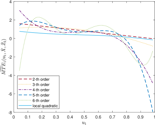
Figure D.1: Specification Checks for the MTE Estimates

Notes: The (instrument-specific) MTE estimates are evaluated at the mean values of $X$ and $Z_{2}$. The MTE estimates in the solid line are based on a local quadratic regression with a Gaussian kernel and a bandwidth of 0.27, using a double residual regression procedure described in Appendix B of Heckman et al. (2006). The bandwidth is picked by Carneiro et al. (2017) using leave-one-out cross-validation. The five other MTE estimates are based on global polynomials in $\hat{p}$ of different orders, with a second-order polynomial (red dashed curve), a third-order polynomial (yellow dotted curve), a fourth-order polynomial (dashes and dots), a fifth-order polynomial (blue dashed curve), and a sixth-order polynomial (green dotted curve).

References

- Athey and Wager (2021) Athey, S. and Wager, S. (2021), “Policy Learning With Observational Data,” Econometrica, 89, 133–161.
- Bertsimas and McCord (2018) Bertsimas, D. and McCord, C. (2018), “Optimization over Continuous and Multi-dimensional Decisions with Observational Data,” in Advances in Neural Information Processing Systems, eds. Bengio, S., Wallach, H., Larochelle, H., Grauman, K., Cesa-Bianchi, N., and Garnett, R., Curran Associates, Inc., vol. 31.
- Bhattacharya and Dupas (2012) Bhattacharya, D. and Dupas, P. (2012), “Inferring Welfare Maximizing Treatment Assignment under Budget Constraints,” Journal of Econometrics, 167, 168–196.
- Björklund and Moffitt (1987) Björklund, A. and Moffitt, R. (1987), “The Estimation of Wage Gains and Welfare Gains in Self-Selection Models,” The Review of Economics and Statistics, 69, 42–49.
- Boucheron et al. (2013) Boucheron, S., Lugosi, G., and Massart, P. (2013), Concentration Inequalities: A Nonasymptotic Theory of Independence, Oxford University Press.
- Brinch et al. (2017) Brinch, C. N., Mogstad, M., and Wiswall, M. (2017), “Beyond LATE with a Discrete Instrument,” Journal of Political Economy, 125, 985–1039.
- Byambadalai (2022) Byambadalai, U. (2022), “Identification and Inference for Welfare Gains without Unconfoundedness,” ArXiv: 2207.04314.
- Carneiro et al. (2010) Carneiro, P., Heckman, J. J., and Vytlacil, E. (2010), “Evaluating Marginal Policy Changes and the Average Effect of Treatment for Individuals at the Margin,” Econometrica, 78, 377–394.
- Carneiro et al. (2011) Carneiro, P., Heckman, J. J., and Vytlacil, E. J. (2011), “Estimating Marginal Returns to Education,” American Economic Review, 101, 2754–81.
- Carneiro and Lee (2009) Carneiro, P. and Lee, S. (2009), “Estimating Distributions of Potential Outcomes Using Local Instrumental Variables with an Application to Changes in College Enrollment and Wage Inequality,” Journal of Econometrics, 149, 191–208.
- Carneiro et al. (2017) Carneiro, P., Lokshin, M., and Umapathi, N. (2017), “Average and Marginal Returns to Upper Secondary Schooling in Indonesia,” Journal of Applied Econometrics, 32, 16–36.
- Chen and Christensen (2015) Chen, X. and Christensen, T. M. (2015), “Optimal Uniform Convergence Rates and Asymptotic Normality for Series Estimators under Weak Dependence and Weak Conditions,” Journal of Econometrics, 188, 447–465, heterogeneity in Panel Data and in Nonparametric Analysis in honor of Professor Cheng Hsiao.
- Chen and Xie (2022) Chen, Y.-C. and Xie, H. (2022), “Personalized Subsidy Rules,” ArXiv: 2202.13545.
- Cornelissen et al. (2016) Cornelissen, T., Dustmann, C., Raute, A., and Schönberg, U. (2016), “From LATE to MTE: Alternative Methods for the Evaluation of Policy Interventions,” Labour Economics, 41, 47–60, sOLE/EALE conference issue 2015.
- Cui and Tchetgen (2021) Cui, Y. and Tchetgen, E. T. (2021), “A Semiparametric Instrumental Variable Approach to Optimal Treatment Regimes Under Endogeneity,” Journal of the American Statistical Association, 116, 162–173, pMID: 33994604.
- Dupas (2014) Dupas, P. (2014), “Short-Run Subsidies and Long-Run Adoption of New Health Products: Evidence From a Field Experiment,” Econometrica, 82, 197–228.
- Heckman et al. (2001) Heckman, J., Tobias, J. L., and Vytlacil, E. (2001), “Four Parameters of Interest in the Evaluation of Social Programs,” Southern Economic Journal, 68, 211–223.
- Heckman et al. (2006) Heckman, J. J., Urzua, S., and Vytlacil, E. (2006), “Understanding Instrumental Variables in Models with Essential Heterogeneity,” The Review of Economics and Statistics, 88, 389–432.
- Heckman and Vytlacil (2001) Heckman, J. J. and Vytlacil, E. (2001), “Policy-Relevant Treatment Effects,” The American Economic Review, 91, 107–111.
- Heckman and Vytlacil (2005) — (2005), “Structural Equations, Treatment Effects, and Econometric Policy Evaluation,” Econometrica, 73, 669–738.
- Heckman and Vytlacil (1999) Heckman, J. J. and Vytlacil, E. J. (1999), “Local Instrumental Variables and Latent Variable Models for Identifying and Bounding Treatment Effects,” Proceedings of the National Academy of Sciences of the United States of America, 96, 4730–4734.
- Hirano and Porter (2009) Hirano, K. and Porter, J. R. (2009), “Asymptotics for Statistical Treatment Rules,” Econometrica, 77, 1683–1701.
- Hirano and Porter (2020) — (2020), “Chapter 4 - Asymptotic Analysis of Statistical Decision Rules in Econometrics,” in Handbook of Econometrics, Volume 7A, eds. Durlauf, S. N., Hansen, L. P., Heckman, J. J., and Matzkin, R. L., Elsevier, pp. 283–354.
- Imbens and Angrist (1994) Imbens, G. W. and Angrist, J. D. (1994), “Identification and Estimation of Local Average Treatment Effects,” Econometrica, 62, 467–475.
- Kallus and Zhou (2018) Kallus, N. and Zhou, A. (2018), “Policy Evaluation and Optimization with Continuous Treatments,” in Proceedings of the Twenty-First International Conference on Artificial Intelligence and Statistics, eds. Storkey, A. and Perez-Cruz, F., PMLR, vol. 84 of Proceedings of Machine Learning Research, pp. 1243–1251.
- Kasy (2016) Kasy, M. (2016), “Partial Identification, Distributional Preferences, and the Welfare Ranking of Policies,” The Review of Economics and Statistics, 98, 111–131.
- Kitagawa and Tetenov (2018a) Kitagawa, T. and Tetenov, A. (2018a), “Supplement to ‘Who Should Be Treated? Empirical Welfare Maximization Methods for Treatment Choice’,” Econometrica Supplemental Material, 86.
- Kitagawa and Tetenov (2018b) — (2018b), “Who Should Be Treated? Empirical Welfare Maximization Methods for Treatment Choice,” Econometrica, 86, 591–616.
- Kédagni and Mourifié (2020) Kédagni, D. and Mourifié, I. (2020), “Generalized Instrumental Inequalities: Testing the Instrumental Variable Independence Assumption,” Biometrika, 107, 661–675.
- Manski (2004) Manski, C. F. (2004), “Statistical Treatment Rules for Heterogeneous Populations,” Econometrica, 72, 1221–1246.
- Mbakop and Tabord-Meehan (2021) Mbakop, E. and Tabord-Meehan, M. (2021), “Model Selection for Treatment Choice: Penalized Welfare Maximization,” Econometrica, 89, 825–848.
- Mogstad et al. (2018) Mogstad, M., Santos, A., and Torgovitsky, A. (2018), “Using Instrumental Variables for Inference About Policy Relevant Treatment Parameters,” Econometrica, 86, 1589–1619.
- Mogstad and Torgovitsky (2018) Mogstad, M. and Torgovitsky, A. (2018), “Identification and Extrapolation of Causal Effects with Instrumental Variables,” Annual Review of Economics, 10, 577–613.
- Mogstad et al. (2021) Mogstad, M., Torgovitsky, A., and Walters, C. R. (2021), “The Causal Interpretation of Two-Stage Least Squares with Multiple Instrumental Variables,” American Economic Review, 111, 3663–98.
- Pu and Zhang (2021) Pu, H. and Zhang, B. (2021), “Estimating Optimal Treatment Rules with an Instrumental Variable: A Partial Identification Learning Approach,” Journal of the Royal Statistical Society: Series B (Statistical Methodology), 83, 318–345.
- Qiu et al. (2021) Qiu, H., Carone, M., Sadikova, E., Petukhova, M., Kessler, R. C., and Luedtke, A. (2021), “Optimal Individualized Decision Rules Using Instrumental Variable Methods,” Journal of the American Statistical Association, 116, 174–191, pMID: 33731969.
- Rubin (1974) Rubin, D. B. (1974), “Estimating Causal Effects of Treatments in Randomized and Nonrandomized Studies,” Journal of Educational Psychology, 66, 688–701.
- Sasaki and Ura (2020) Sasaki, Y. and Ura, T. (2020), “Welfare Analysis via Marginal Treatment Effects,” ArXiv: 2012.07624.
- Sasaki and Ura (2021) — (2021), “Estimation and Inference for Policy Relevant Treatment Effects,” Journal of Econometrics.
- Sun (2021) Sun, L. (2021), “Empirical Welfare Maximization with Constraints,” ArXiv: 2103.15298.
- Thornton (2008) Thornton, R. L. (2008), “The Demand for, and Impact of, Learning HIV Status,” American Economic Review, 98, 1829–63.
- van der Vaart and Wellner (1996) van der Vaart, A. and Wellner, J. (1996), Weak Convergence and Empirical Processes: With Applications to Statistics, Springer Series in Statistics, Springer.
- Vytlacil (2002) Vytlacil, E. (2002), “Independence, Monotonicity, and Latent Index Models: An Equivalence Result,” Econometrica, 70, 331–341.
- Wang and Tchetgen Tchetgen (2018) Wang, L. and Tchetgen Tchetgen, E. (2018), “Bounded, Efficient and Multiply Robust Estimation of Average Treatment Effects Using Instrumental Variables,” Journal of the Royal Statistical Society: Series B (Statistical Methodology), 80, 531–550.