Spectra of generators of Markovian evolution in the thermodynamic limit: From non-Hermitian to full evolution via tridiagonal Laurent matrices

Abstract

We determine spectra of single-particle translation-invariant Lindblad operators on the infinite line. In the case where the Hamiltonian is given by the discrete Laplacian and the Lindblad operators are rank $r$, finite range and translates of each other, we obtain a representation of the Lindbladian as a direct integral of finite range bi-infinite Laurent matrices with rank-$r$-perturbations. By analyzing the direct integral we rigorously determine the spectra in the general case and calculate it explicitly for several types of dissipation e.g. dephasing, and coherent hopping. We further use the detailed information about the spectrum to prove gaplessness, absence of residual spectrum and a condition for convergence of finite volume spectra to their infinite volume counterparts. We finally extend the discussion to the case of the Anderson Hamiltonian, which enables us to study a Lindbladian recently associated with localization in open quantum systems.

1 Introduction

Schrödinger operators and their spectra are one of the central objects studied in mathematical physics. Indeed, spectral properties encode many important physical properties such as the speed of propagation as described by the RAGE theorem [2, 3, 4].

Going beyond the closed system paradigm described by Schrödinger operators and unitary dynamics, a natural setting is that of Markovian time-evolution, described by a completely positive dynamical semi-group. These systems have been extensively studied from a quantum information perspective in particular by considering the generator of such evolutions, i.e. the Lindblad generator [5]. Here, gaps in the spectrum around the origin in the complex plane provide information about relaxation times towards the non-equilibrium steady state of the system (as we will discuss in Section 2.2). Understanding the interplay between disorder (e.g. in the form of a random potential) and dissipation (e.g. thermal noise) is emerging as an important problem [6, 7, 8, 9]

In addition, over the past decades, the theory of non-Hermitian Hamiltonians (i.e Non-self-adjoint Schrödinger operators) has developed rapidly [10, 11, 12, 13]. One motivation for these investigations has been that non-Hermitian Hamiltonians model open quantum systems if quantum jumps are neglected [14]. The theory of non-Hermitian Hamiltonians is also closely connected to the study of tridiagonal Laurent matrices (see [15, 16, 17] and references therein). In particular, the stability of the spectra under perturbations has been investigated [18].

In this paper, we extend this connection to the case of Markovian evolution in the single particle regime (illustrated in Figure 1). For Lindbladians with translation-invariant Hamiltonians and Lindblad operators $L_{k}$ that are rank-one, finite range and translates of each other we prove in Theorem 3.8 that the entire Lindbladian can be rewritten as a direct integral of tridiagonal Laurent matrices $T(q)$ corresponding to the non-Hermitian evolution subject to a rank-one perturbation $F(q)$ which corresponds to the quantum jump terms. The construction of $T(q)$ and $F(q)$ is explicit. This decomposition allows us to explore the spectral effects of the quantum jumps rigorously.

The Lindbladian $\mathcal{L}$ is non-normal and so the notion pseudo-spectrum provides information about the operator in not encoded in the spectrum as discussed in great detail in [19, 10]. To determine the spectrum of the Lindbladian from the direct integral decomposition we extend the use of pseudo-spectra by providing a result of independent interest concerning the spectrum of a direct integral in terms of the pseudo-spectra of its fibers and thereby generalizing the corresponding result for the direct sum [20]. This is the content of Theorem 3.12.

The combination of the direct integral decomposition and Theorem 3.12 enables us to obtain information about the spectrum of the Lindbladian $\mathcal{L}$.

In Section 4 we discuss some abstract consequences of the direct integral decomposition. First, we use the decomposition to prove that Lindbladians in the class we consider only have approximate point spectrum. Second, we discuss convergence of finite volume spectra to their infinite volume counterparts and finally we prove that the Lindbladians in question are always gapless or have an infinite dimensional kernel.

In Section 5, we then use the direct integral decomposition more concretely to completely determine the spectrum of some Lindbladians which have received attention in the physics literature as the one-particle sector of open spin chains [21, 22, 23] thereby complementing the exact results on the spectrum from [24]. We are particularly interested in an example where the dissipators are non-normal and where the system shows signs of localization in an open quantum system [25]. Our rigorous analytic results also complement the large body of very recent work on random Lindblad operators studied from a random matrix theory point of view [26, 27, 28, 29].

Finally, to connect to examples to the open quantum system with disorder, in Theorem 6.1 we prove a Lindbladian analogue of the Kunz-Soulliard theorem from the theory of random operators.

In contrast to many previous investigations, we work directly on the entire lattice $\mathbb{Z}$. That allows us to utilise translation-invariance, Laurent matrices and some tools from random operator theory that do not work for finite systems. Furthermore, working in infinite volume directly allows us to determine closed formulas for the spectra explicitly. From one point of view, one can look at these formulas as approximations to (some) large finite-volume systems. In Theorem 4.5 we give conditions that ensure this convergence.

With some exceptions, [30, 31, 32, 7, 9], the study of Lindbladian evolutions has, in recent decades, focused on finite spin systems. We therefore first present some results with conditions for the Lindbladian $\mathcal{L}$ to be bounded as an operator on respectively the space of bounded, Hilbert-Schmidt and trace-class operators.

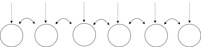
Figure 1: An example of the systems that we discuss in the following. We have a single particle on a lattice with hopping between lattice sites and local dissipation. In this example, the hopping and dissipation have the shortest possible range, but the methods presented apply as long as these properties stay local.    

2 Lindblad systems on the infinite lattice 

We consider the Markovian, open-system dynamics of a single quantum particle on the one-dimensional lattice described by the Hilbert space $\mathcal{H}=\ell^{2}(\mathbb{Z})$ and a distinguished (position) basis $\{{|{k}\rangle}\}_{k\in\mathbb{Z}}$.

The underlying completely positive dynamical semi-group is generated by a Lindbladian $\mathcal{L}:\mathcal{B}(\mathcal{H})\to\mathcal{B}(\mathcal{H})$ of the form [33, 5]

$$\mathcal{L}(\rho)=-i[H,\rho]+G\sum_{k}L_{k}\rho L_{k}^{*}-\frac{1}{2}(L_{k}^{*}L_{k}\rho+\rho L_{k}^{*}L_{k}),$$ (1)

where $H$ is the Hamiltonian of the system (a self-adjoint bounded operator) and $G>0$ is the coupling constant of the dissipation and we have used $A^{*}$ to denote the adjoint of an operator $A$. We will refer to the second term as the dissipative part. The operators $L_{k}\in\mathcal{B}(\mathcal{H})$ implementing the dissipative part are referred to as Lindblad operators. The semi-group determines the time-evolution of a state $\rho(t)$ at time $t\geq 0$, which is given by

$$\rho(t)=e^{t\mathcal{L}}(\rho_{0}),$$

where $\rho(0)=\rho_{0}$ is the state at time $t=0$.

Later, we will often choose our $L_{k}$ to act locally as for example $L_{k}={|{k}\rangle}{\langle{k}|}$. In the following, we will refer to (1) as the Lindblad form. We will similarly say that an operator $\tilde{\mathcal{L}}$ is in the adjoint Lindblad form if

$$\tilde{\mathcal{L}}(X)=i[H,X]+G\sum_{k}L_{k}^{*}XL_{k}-\frac{1}{2}(L_{k}^{*}L_{k}X+XL_{k}^{*}L_{k}),$$ (2)

which describes the evolution of observables in the Heisenberg picture, whereas the evolution generated on states according to (1) is refered to as the Schrödinger picture. The case of a Markovian evolution on the infinite line is slightly under-represented in the literature as many works, in particular from the quantum information side, where open-system dynamics has been studied extensively, restrict themselves to finite dimensions. The infinite case adds some additional complications that we clarify without using the lattice structure of $\ell^{2}(\mathbb{Z})$.

Oftentimes, we will use a decomposition of $\mathcal{L}$ in terms of a non-Hermitian evolution part $\mathcal{L}_{\operatorname*{NHE}}$ and a quantum jump term $\mathcal{L}_{J}$ according to

$$\mathcal{L}(\rho)=-i(H_{\operatorname*{eff}} \rho-\rho H_{\operatorname*{eff}}^{*})+G\sum_{k}L_{k}^{*}\rho L_{k}=\mathcal{L}_{\operatorname*{NHE}}(\rho)+\mathcal{L}_{J}(\rho).$$

where $\mathcal{L}_{J}(\rho)=G\sum_{k}L_{k}^{*}\rho L_{k}$ and the effective non-Hermitian Hamiltonian is defined by

$$H_{\operatorname*{eff}} =H- \frac{iG}{2} \sum_{k}L_{k}^{*}L_{k}.$$ (3)

The Lindblad form ensures that the spectrum is always contained within the half-plane of the complex plane with non-positive real part (see also [34, 35]).

Furthermore, for finite-dimensional systems $\mathcal{L}(X^{*})=\mathcal{L}(X)^{*}$ which implies that the spectrum is invariant under complex conjugation $\sigma(\mathcal{L})=\overline{\sigma(\mathcal{L})}$. This we prove also in the infinite-dimensional case in Lemma A.4.

In finite dimensions, it is always the case that there is a steady state $\rho_{\infty}$ of the dynamics that satisfies $\mathcal{L}(\rho_{\infty})=0$ (see for example [35, Proposition 5]). It was discussed in [36, 37, 38, 39] how the symmetries of $L_{k}$ are inherited by $\mathcal{L}$ and the steady state. However, translation invariant infinite volume Lindbladians have not been studied extensively although some results exist [40, 7].

2.1 Boundedness of $\mathcal{L}$ as an operator on Schatten spaces

In finite dimensions, the set of density matrices is defined to be the set of positive matrices with unit trace. In infinite dimensions, this notion is generalised to positive trace-class operators with unit trace. In the following, we will denote the space of trace-class operators by $\operatorname*{TC}(\mathcal{H})$, the Hilbert-Schmidt operators by $\operatorname*{HS}(\mathcal{H})$ and the space of bounded operators by $\mathcal{B}(\mathcal{H})$. See for example [10, 41] for more details on these spaces. All three spaces are Banach spaces with regards to their respective norms and $\operatorname*{HS}(\mathcal{H})$ is also a Hilbert space with the inner product

$$\langle X,Y\rangle=\Tr(X^{*}Y).$$

In order to relate the spectra of $\mathcal{L}$ on these different Banach spaces, we will use interpolation methods. These methods rely on the Schatten classes that interpolate between $\operatorname*{TC}(\mathcal{H}),\operatorname*{HS}(\mathcal{H})$ and $\mathcal{B}(\mathcal{H})$. To define them we consider operators $A\in\mathcal{B}(\mathcal{H})$ with and define for $p\in(1,\infty)$ the Schatten-$p$-norm of $A$ via

$$\norm{A}_{p}=\Tr(\absolutevalue{A}^{p})^{\frac{1}{p}},$$

where $\absolutevalue{A}=(AA^{*})^{\frac{1}{2}}$. The Schatten-$p$-class $\mathcal{S}_{p}$ then consists of all bounded operators with finite $p$-norm. For $p=\infty$ we set $\mathcal{S}_{\infty}=\mathcal{K}(\mathcal{H})$, the compact operators on $\mathcal{H}$. Furthermore, the Schatten classes interpolate between these spaces in the sense that $\mathcal{S}_{1}=\operatorname*{TC}(\mathcal{H}),\mathcal{S}_{2}=\operatorname*{HS}(\mathcal{H})$. For more information see [42] where the Schatten classes are treated extensively.

We first show that under a boundedness assumption on the $L_{k}$ any Lindblad generator of the form (1) will be a bounded operator on $\operatorname*{TC}(\mathcal{H}),\operatorname*{HS}(\mathcal{H})$ as well as $\mathcal{B}(\mathcal{H})$. To this end, assume that $H\in\mathcal{B}(\mathcal{H})$ and that

$$(\mathcal{A}_{1}):\text{ Both  }\left\{\sum_{k\in\mathbb{Z}:\absolutevalue{k}\leq n} L_{k}L_{k}^{*}\right\}_{n\in\mathbb{N}}\text{ and }\left\{\sum_{k\in\mathbb{Z}:\absolutevalue{k}\leq n} L_{k}^{*}L_{k}\right\}_{n\in\mathbb{N}}\text{ converge weakly }\text{in }\mathcal{B}(\mathcal{H}),$$

where we recall a sequence of operators $\{A_{n}\}_{n\in\mathbb{N}}\subset\mathcal{B}(\mathcal{H})$ converges weakly to an operator $A\in\mathcal{B}(\mathcal{H})$ if for all $v\in\mathcal{H}$ it holds that $\norm{A_{n}v-Av}\to 0$.

A similar level of generality was used in [43] and [44]. We will use the Riesz-Thorin interpolation theorem in a non-commutative version, where the operators are defined on the Schatten classes $\mathcal{S}_{p}$. We state it here for convenience.

We say that a pair of operators $A_{p}\in\mathcal{B}(\mathcal{S}_{p})$ and $A_{q}\in\mathcal{B}(\mathcal{S}_{q})$ are defined consistently if for any $\rho\in\mathcal{S}_{p}\cap\mathcal{S}_{q}$ it holds that $A_{p}\rho=A_{q}\rho$. If this is the case, we abuse notation by writing $A\in\mathcal{B}(\mathcal{S}_{p}),\mathcal{B}(\mathcal{S}_{q})$. Notice that since the Lindbladian is defined through the Lindblad form (1) for some fixed operators $H,L_{k}$. Then $\mathcal{L}$ is consistently defined and we abuse notation by writing both $\mathcal{L}\in\mathcal{B}(\mathcal{S}_{p})$ and $\mathcal{L}\in\mathcal{B}(\mathcal{S}_{q})$, whenever it is the case.

Theorem 2.1 ([45, Section IX.4]).

Let $p,q\geq 1$ and $A\in\mathcal{B}(\mathcal{S}_{p}),\mathcal{B}(\mathcal{S}_{q})$ consistently, then $A\in\mathcal{B}(\mathcal{S}_{r_{t}})$ where $\frac{1}{r_{t}} =\frac{t}{p} +\frac{1-t}{q}$ for each $t\in[0,1]$ with

$$\norm{A}_{r_{t}\to r_{t}} \leq\norm{A}_{p\to p}^{t}\norm{A}_{q\to q}^{1-t}.$$

The theorem enables us to prove that Assumption $(\mathcal{A}_{1})$ is enough to ensure boundedness on all Schatten spaces, but we state the more relevant ones here for clarity.

Lemma 2.2.

Suppose that $\mathcal{L}$ is of the Lindblad form (1) and that $(\mathcal{A}_{1})$ holds. Then

$$\mathcal{L}\in\mathcal{B}(\mathcal{B}{(\mathcal{H})}),\mathcal{B}(\operatorname*{HS}(\mathcal{H})),\mathcal{B}(\operatorname*{TC}(\mathcal{H})).$$

This is also true if $\mathcal{L}$ is of the adjoint Lindblad form (2).

Proof.

The case $\mathcal{L}\in\mathcal{B}(\operatorname*{TC}(\mathcal{H}))$ follows from [44, prop 6.4]. In Appendix A.2 we prove that $\mathcal{L}\in\mathcal{B}(\mathcal{B}{(\mathcal{H})})$. Then, to see that $\mathcal{L}\in\mathcal{B}(\operatorname*{HS}(\mathcal{H}))$ we use the non-commutative Riesz-Thorin theorem. Note that since the operator $\mathcal{L}$ is bounded on $\mathcal{B}{(\mathcal{H})}$ it is also bounded as an operator on the compact operators $\mathcal{K}{(\mathcal{H})}=\mathcal{S}_{\infty}$. Thus, we obtain that

$$\norm{\mathcal{L}}_{2\to 2} \leq\norm{\mathcal{L}}_{1\to 1}^{\frac{1}{2}}\norm{\mathcal{L}}_{\infty\to\infty}^{\frac{1}{2}}.$$

This shows that $\mathcal{L}\in\mathcal{B}(\operatorname*{HS}(\mathcal{H}))$. For further discussions and similar results see also [46, 47]. The result for the adjoint Lindblad form follows in the same way because of the assumption $(\mathcal{A}_{1})$. ∎

We have now proven that the Lindbladian $\mathcal{L}$ is an element of the Banach algebras $\mathcal{B}(\operatorname*{TC}(\mathcal{H})),$ $\mathcal{B}(\operatorname*{HS}(\mathcal{H}))$ and $\mathcal{B}(\mathcal{B}(\mathcal{H}))$, where $\mathcal{B}(\operatorname*{HS}(\mathcal{H}))$ is also a $C^{*}$-algebra.

In the main text we will only consider the case $\mathcal{B}(\operatorname*{HS}(\mathcal{H}))$. In particular, we only determine the spectrum exactly there. But in Appendix A.1 we make some remarks on spectral independence of Lindblad operators.

In the following, we will be concerned with the spectrum of $A$ in each of these algebras. For any Banach algebra $\mathcal{A}$ the spectrum of an operator $A$ with respect to the algebra $\mathcal{A}$ is defined as follows

$$\sigma_{\mathcal{A}}(A)=\{\lambda\in\mathbb{C}\mid A-\lambda\text{ is not invertible in }\mathcal{A}\}.$$

Furthermore, we define the approximate point spectrum of an operator in a Banach algebra $\mathcal{A}=\mathcal{B}(X)$ for some Banach space $(X,\norm{\cdot}_{X})$, is given by

$$\sigma_{\mathcal{A},\operatorname*{appt}}(A)=\{\lambda\in\mathbb{C}\mid\exists(\psi_{n})_{n\in\mathbb{N}}\subset X,\norm{\psi_{n}}_{X}=1,\lim_{n\to\infty} \norm{ (A-\lambda)\psi_{n}}_{X}=0\}.$$

A sequence $(\psi_{n})_{n\in\mathbb{N}}$ corresponding to a point $\lambda\in\mathbb{C}$ as above we will call a Weyl sequence corresponding to $\lambda$. It is always the case that $\sigma_{\mathcal{A},\operatorname*{appt}}(A)\subset\sigma_{\mathcal{A}}(A)$ and for normal operators equality holds [41, 12.11]. We will prove in Theorem 4.1 that the equality also holds in many of our cases of interest. The set

$$\sigma_{\mathcal{A},\operatorname*{res}}(A)=\sigma_{\mathcal{A}}(A)\backslash\sigma_{\mathcal{A},\operatorname*{appt}}(A)$$

is called the residual spectrum of $A$.

In the following, we will be particularly interested in the case where the Banach algebra $\mathcal{A}=\mathcal{B}(\mathcal{S}_{p})$. It is a classical result that $\mathcal{S}_{p}$ (and in turn $\mathcal{A}$) is Banach algebra in itself, and that $\mathcal{S}_{p}$ is an ideal in $\mathcal{B}(\mathcal{H})$ for all $p\in[1,\infty]$. The Calkin algebra $\mathcal{Q}(\mathcal{H})$ is defined by $\mathcal{Q}(\mathcal{H})=\mathcal{B}(\mathcal{H})\backslash\mathcal{K}(\mathcal{H})$ and the spectrum of an operator $A$ in the Calkin algebra we call the essential spectrum $\sigma_{\operatorname*{ess}}(A)=\sigma_{\mathcal{Q}(\mathcal{H})}(A)$.

In the following, we are mainly concerned with translation-invariant operators with finite range. We formalize this by the following two assumptions.

$$\text{ $(\mathcal{A}_{2}a):\text{  }$ \emph{Finite range $r<\infty$ }: ${\langle{y}|},L_{k}{|{x}\rangle}=0$ whenever $\max\{\absolutevalue{x-k},\absolutevalue{y-k}\} >r$}$$

$$(\mathcal{A}_{2}b):\text{  } S_{1}L_{k}S_{-1}=L_{k+1} k\in\mathbb{Z}$$ Translation-invariance: for each

where the operator $S_{n}$ on $\mathcal{H}$ is defined by $(S_{n}\psi)(x)=\psi(x-n)$ with the convention that $S=S_{1}$. Notice that since $\mathcal{H}=\ell^{2}(\mathbb{Z})$ the operator $S_{n}$ is unitary and $S_{n}^{-1} =S_{n}^{*}=S_{-n}$.

If we further assume that the Hamiltonian $H$ is translation-invariant meaning that $H=S_{1}HS_{1}^{*}$, then Assumption $(\mathcal{A}_{2}b)$ implies that $\mathcal{L}$ is translation-covariant, i.e. it satisfies that

$$\mathcal{L}(S_{1}\rho S_{1}^{*})=S_{1} \mathcal{L}(\rho)S_{1}^{*}.$$ (4)

It is easy to see that (4) implies that $\mathcal{L}(S_{n}\rho S_{n}^{*})=S_{n} \mathcal{L}(\rho)S_{n}^{*}$ for all $n\in\mathbb{Z}$. Furthermore, it is also true that $(\mathcal{A}_{2}a)$ and $(\mathcal{A}_{2}b)$ imply $(\mathcal{A}_{1})$. To see this, notice that $(\mathcal{A}_{2}b)$ implies that $\sum_{k}L_{k}L_{k}^{*}$ is translation-invariant and therefore constant on diagonals. Now, $(\mathcal{A}_{2}a)$ implies that there are only finitely many non-zero diagonals and the diagonal entries are finite. Thus, $\sum_{k}L_{k}L_{k}^{*}=\sum_{n=-r}^{r}\alpha_{n}S_{n}$ for $\alpha_{n}\in\mathbb{C}$ for $-r\leq n\leq r$, which is a bounded operator.

2.2 Relation between spectra and dynamics for Lindblad systems

In the rest of the paper, our focus will be on determining the spectra of certain infinite-volume open quantum systems. In the Hamiltonian case, there is a clear dynamical interpretation of the spectra and the different types of spectra. However, due to non-normality of Lindblad operators, the dynamical implications of the spectra are more subtle and the details of the topic are still under discussion in the physics literature [49]. We discuss our knowledge in both finite and infinite dimensional cases.

Finite dimensions: In the finite-dimensional, case the relationship between eigenvalues of $\mathcal{L}$ and the time evolution is given through the Jordan normal form. I.e. $\mathcal{L}=S\Lambda S^{-1}$ where $S$ is invertible and $\Lambda$ is of a certain almost-diagonal form. However, even in the cases where $\Lambda$ is diagonal, $\mathcal{L}$ is not necessarily normal. The analysis is counter-intuitive to the person trained in Hamiltonian formalism due to the peculiarities of non-normality. In particular, the mathematical guarantees for convergence of the semigroup are much much weaker in the normal case and they scale much worse with the dimension of the system (see e.g. [50]).

Another peculiarity is the fact that all eigenvectors of $\mathcal{L}$ are traceless, which we describe in the following remark.

Remark 2.3.

All eigenvectors of $\mathcal{L}$ with eigenvalues not equal to 0 are traceless. To see that, note that $e^{t\mathcal{L}}$ is trace-preserving for all $t\in[0,\infty)$, so it holds that

$$\Tr(\rho)=\Tr\left(e^{t\mathcal{L}}(\rho)\right)=e^{\lambda t}\Tr(\rho).$$

Thus, if $\Tr(\rho)\neq 0$ then for all $t\in[0,\infty)$ we get $1=e^{\lambda t}$ which implies that $\lambda=0$.

We can give guarantees about the dynamics in terms of the spectral gap $g$ of $\mathcal{L}$ which we define as follows

$$g=\sup\left\{\text{Re}(\lambda)\mid\lambda\in\sigma(\mathcal{L})\backslash\{0\}\right\}.$$

In the case where we have a unique steady state $\rho_{\infty}$, we can get a dynamical guarantee for the speed of decay towards the steady state in terms of the gap $g$. Namely that $\norm{e^{t\mathcal{L}}(\rho)-\rho_{\infty}}\leq Ce^{tg}$ where $C>0$ is a constant that depends heavily on the size of the Jordan blocks of the systems.

In the literature, the cases where $\mathcal{L}$ is not diagonalizable are called exceptional points, there is evidence that these points can also lead to faster decay towards the steady state [51], although the mathematical guarantee gets worse. 

Infinite dimensions:  In infinite dimensions the relationship between spectra and dynamics can break down due to Jordan blocks of unbounded size (and more generally the breakdown of the Jordan normal form), due to the lack of a trace class steady state (a phenomenon that we will encounter in most examples in Section 5) and due to the lack of a spectral gap (which we prove for our models in Theorem 4.10).

However, we will encounter situations where $\sigma(\mathcal{L})$ has two or more disconnected parts. Suppose for simplicity that we just have two parts $\sigma(\mathcal{L})=\Sigma_{A}\dot{\cup}\Sigma_{B}$, with $\sup\{\real(z)\mid z\in\Sigma_{A}\} \leq g$ for some gap $g\in(-\infty,0)$ and such that there exists is a closed continuous curve encircling only $\Sigma_{A}$. Then we can define the Riesz projections by contour integration to get a decomposition of $\mathcal{H}=\mathcal{H}_{A}\oplus\mathcal{H}_{B}$ for two orthogonal subspaces $\mathcal{H}_{A},\mathcal{H}_{B}$ such that $\mathcal{L}$ leave each of the two subspaces invariant. Thus, we can decompose $\mathcal{L}=\mathcal{L}_{A}\oplus\mathcal{L}_{B}$. Suppose that $\rho\in\mathcal{H}_{A}$ then, since $\mathcal{L}_{A}$ is the generator of a semigroup by [52], it holds that

$$\norm{e^{t\mathcal{L}}(\rho)}= \norm{e^{t\mathcal{L}_{A}}(\rho)}\leq Ce^{tg} \norm{\rho}$$

for some constant $C>0$. Thus, if $\rho=\rho_{A}+\rho_{B}$ with $\rho_{A}\in\mathcal{H}_{A}$ and $\rho_{B}\in\mathcal{H}_{B}$ we see that the part $\rho_{A}$ decays quickly.

We leave it to future work to establish a stronger relationship between spectra and dynamics in the infinite-dimensional case. In particular, one cannot use our work to gain many rigorous guarantees about the evolution of infinite open quantum systems, but we consider the results presented as steps towards such rigorous guarantees. Furthermore, due to the apparent convergence of the spectra of some finite-dimensional Lindbladians (see Theorem 4.5 and the discussion in Section 7) one can also view the method presented here as a way to compute large volume approximations to finite systems (which have discrete spectra and where the relation between spectra and dynamics is clearer).

In fact, given the question on spectral independence raised in the previous section one might even ask which Banach algebra (potentially $\mathcal{B}(\mathcal{S}_{p})$ for some $p\in[1,\infty]$) enables us to transfer knowledge from spectra to dynamics of states $\rho\in\mathcal{S}_{1},\rho\geq 0$ and $\Tr(\rho)=1$.

3 Direct integral decompositions and their spectra  

In this section, we specialize to the case where the Hamiltonian $H\in\mathcal{B}\left(l^{2}(\mathbb{Z})\right)$ is the discrete Laplacian $-\Delta$ defined in (38). From now on, we will use Dirac notation, to do that we define for a $k\in\mathbb{Z}$ the vector ${|{k}\rangle}=e_{k}$, and we let ${\langle{k}|}$ be the corresponding dual vector. On caveat here is that since we will be working with non-selfadjoint operators, then ${\langle{k}|},A{|{k^{\prime}}\rangle}\neq{\langle{k}|}A,{|{k^{\prime}}\rangle}$ and therefore the comma in the inner product is important and we write it consistently.

Since $H$ only enters through into the Lindbladian given by (1) the commutator $[H,\cdot]$ does not change when disregarding the term $-2{|{k}\rangle}{\langle{k}|}$. Thus, we will often work with

$$H=-\tilde{\Delta}=-\sum_{k\in\mathbb{Z}}\outerproduct{k}{k+1} + \outerproduct{k+1}{k}=-(S+S^{*}),$$ (5)

where the operator $S_{n}$ on $\mathcal{H}$ was defined by $(S_{n}\psi)(x)=\psi(x-n)$ and we used the convention that $S=S_{1}$ for the shift operator. For the Lindblad operators $L_{k}$, we made the following assumptions in the previous section.

$$\text{ $(\mathcal{A}_{2}a):\text{  }$ \emph{Finite range $r<\infty$ }: ${\langle{y}|},L_{k}{|{x}\rangle}=0$ whenever $\max\{\absolutevalue{x-k},\absolutevalue{y-k}\} >r$.}$$

$$(\mathcal{A}_{2}b):\text{  } S_{n}L_{k}S_{-n}=L_{k+n}$$ Translation-invariance: .

Sometimes, we will also need the assumption

$$(\mathcal{A}_{2}c):\text{  } \text{Rank}(L_{k})=1$$ rank-one: .

Notice that in particular, we do not assume that each of the $L_{k}$ is normal or self-adjoint and in fact, one of our motivating examples has non-normal $L_{k}$. Notice that $H$ is translation-invariant in the sense that $H=S_{n}HS_{n}^{*}$. The assumption $(\mathcal{A}_{2}b)$ implies that $\mathcal{L}$ is translation-covariant in the sense of (4).

We will use a sequence of isometric isomorphisms of Hilbert spaces to obtain our main result. Therefore we briefly recall some facts about them. We call a map between separable Hilbert spaces $U:\mathcal{H}_{1}\to\mathcal{H}_{2}$ an isometric isomorphism if it is linear, bijective and preserves the inner product $\langle U(x),U(y)\rangle_{\mathcal{H}_{2}} =\langle x,y\rangle_{\mathcal{H}_{1}}.$ We recall that every isometric isomorphism of separable Hilbert spaces is a unitary operator [53, Theorem 5.21] . Now, $U$ gives rise to an isomorphism $C^{*}$-algebras $U^{\uparrow}:\mathcal{B}(\mathcal{H}_{1})\to\mathcal{B}(\mathcal{H}_{2})$ given by conjugation

$$U^{\uparrow}(A)=UAU^{*}.$$ (6)

Where we have introduced the notation $U^{\uparrow}$ since we will compose many isomorphisms the reader should notice that

$$(UV)^{\uparrow}=U^{\uparrow}V^{\uparrow}.$$ (7)

3.1 Review of Fourier transformations and symbol curves for Laurent operators

We will use the Fourier transformation extensively and therefore we review it before continuing. Following the normalization convention in [1, (A.9)] we let $\mathcal{F}:\ell^{2}(\mathbb{Z})\to L^{2}([0,2\pi])$ be defined by

$$(\mathcal{F}\psi)(q)=\frac{1}{\sqrt{2\pi}}\sum_{x\in\mathbb{Z}} e^{-iqx}\psi(x),$$

for any $\psi\in\ell^{2}(\mathbb{Z})$. Then $\mathcal{F}$ is unitary and its adjoint, the inverse Fourier transform, $\mathcal{F}^{-1}:L^{2}([0,2\pi])\to\ell^{2}(\mathbb{Z})$ is given by

$$(\mathcal{F}^{-1}\varphi)(x)=\frac{1}{\sqrt{2\pi}}\int_{0}^{2\pi} e^{iqx}\varphi(q)dq,$$ (8)

for every $\varphi\in L^{2}([0,2\pi])$. We summarise these observations as follows.

Theorem 3.1.

The operator $\mathcal{F}:\ell^{2}(\mathbb{Z})\to L^{2}([0,2\pi])$ is a well defined bounded operator and it is an isometric isomorphism. For the operator $\mathcal{F}^{-1}:L^{2}([0,2\pi])\to\ell^{2}(\mathbb{Z})$ defined by (8) satisfies $\mathcal{F}^{-1}=\mathcal{F}^{*}$ as well as

$$\mathcal{F}\mathcal{F}^{-1}=1\!\!1_{L^{2}([0,2\pi])} \text{ and } \mathcal{F}^{-1}\mathcal{F}=1\!\!1_{\ell^{2}(\mathbb{Z})}.$$

Furthermore, $\mathcal{F}$ maps the standard basis $\{{|{j}\rangle}\}_{j\in\mathbb{Z}}$ to the Fourier basis consisting of functions $\{\frac{1}{\sqrt{2\pi}}e^{-ikj}\}_{j\in\mathbb{Z}}$. It is standard that if $T$ is a translation invariant operator on $\ell^{2}(\mathbb{Z})$ (defined as $STS^{*}=T$). Then the corresponding operator $\mathcal{F}T\mathcal{F}^{-1}\in\mathcal{B}(L^{2}([0,2\pi]))$ will be a multiplication operator.

The Fourier transform transforms Laurent operators into multiplication operators, so we briefly recall the definition of a Laurent operator. A Laurent operator $T\in\mathcal{B}(\ell^{2}(\mathbb{Z}))$ is an operator if for all $i,j,n\in\mathbb{Z}$ it holds ${\langle{i}|},T{|{j}\rangle}={\langle{i+n}|},L{|{j+n}\rangle}$, thus, in position basis, we can write $T$ as a bi-infinite matrix that is constant on the diagonals.

$$T=\begin{pmatrix}\dots&\dots&\dots&\dots&\dots\\ \dots&a_{0}&a_{1}&a_{2}&\dots\\ \dots&a_{-1}&a_{0}&a_{1}&\dots\\ \dots&a_{-2}&a_{-1}&a_{0}&\dots\\ \dots&\dots&\dots&\dots&\dots\end{pmatrix}.$$

In other words, $T$ is a banded matrix. If $a_{n} =0$, whenever $\absolutevalue{n}>r$ we say that $T$ is r-diagonal. In that case,

$$T=\sum_{i=-r}^{r}a_{i}S_{i}.$$

Lemma 3.2.

Suppose that $T\in\mathcal{B}(\ell^{2}(\mathbb{Z}))$ is translation invariant with constant entries $a_{i}$ on the $i$-th diagonal and $a_{i}=0$ for $\absolutevalue{i} \geq r$. Then the Fourier transform of $T$ is defined by

$$\mathcal{F}T\mathcal{F}^{*}\in\mathcal{B}(L^{2}([0,2\pi]))$$

is a multiplication operator multiplying with $a_{T}(q)=\sum_{j=-r}^{r}a_{j}e^{iqj}$. In particular, if $S$ is the shift operator then

$$\mathcal{F}^{\uparrow}(S)=\mathcal{F}S\mathcal{F}^{*}=e^{-iq}$$

as an operator on $L^{2}([0,2\pi])$.

Proof.

Consider for any $j\in\mathbb{Z}$ the operator $T=\sum_{n\in\mathbb{Z}}{|{n}\rangle}{\langle{n+j}|}=S_{-j}$. Then for $q\in[0,2\pi]$ it holds for any $\phi\in L^{2}([0,2\pi])$ that

$$(\mathcal{F}T\mathcal{F}^{*}\phi)(q)=\frac{1}{\sqrt{2\pi}}\sum_{x\in\mathbb{Z}} e^{-iqx}(T\mathcal{F}^{*}\phi)(x) =\frac{1}{\sqrt{2\pi}}\sum_{x\in\mathbb{Z}} e^{-iqx}(\mathcal{F}^{*}\phi)(x+j)$$ (9)

$$=\frac{1}{\sqrt{2\pi}}\sum_{x\in\mathbb{Z}} e^{-iqx}\frac{1}{\sqrt{2\pi}}\int_{[0,2\pi]} e^{iq^{\prime}(x+j)}\phi(q^{\prime})dq^{\prime}$$ (10)

$$=e^{iqj}\phi(q),$$ (11)

where we used Plancherel’s Theorem in the last step. Now, by linearity if

$$T=\sum_{j=-r}^{r}a_{j}\sum_{n\in\mathbb{Z}}{|{n}\rangle}{\langle{n+j}|},$$

it holds that

$$(\mathcal{F}T\mathcal{F}^{*}\phi)(q)=\left(\sum_{j=-r}^{r}a_{j}e^{iqj}\right)\phi(q).$$

∎

The curve $a_{T}(k)=\sum_{j=-r}^{r}a_{j}e^{iqj}$ can also be viewed as a function from the unit circle defining $z=e^{iq}$, then $a_{T}(z)=\sum_{j=-r}^{r}a_{j}z^{j}$ we denote this curve the symbol curve. Since the Fourier transformation is unitary and using that the essential spectrum is the part of the spectrum that is not isolated eigenvalues with finite multiplicity [54, IV.5.33] we obtain the following corollary.

Corollary 3.3.

For any Laurent operator $T\in\mathcal{B}(\ell^{2}(\mathbb{Z}))$ it holds that

$$\sigma(T)=\{a_{T}(z)\mid z\in\mathbb{T}\}=\sigma_{\operatorname*{ess}}(T).$$

Furthermore, as explained in [55, Theorem 1.2] if $0\not\in\sigma(T)$ then the inverse of $T$ is unitarily equivalent to a multiplication with the inverse symbol

$$a_{T^{-1}}(z)=a_{T}^{-1}(z)=\frac{1}{a_{T}(z)}.$$

In concrete applications, we consider tridiagonal matrices $T(q)$ and therefore, we review some results about tridiagonal Laurent operators and their invertibility in Appendix A.7. If $T(q)$ is tridiagonal we let $\alpha,\beta,\gamma:[0,2\pi]\to\mathbb{C}$ be the entries of $T(q)$. Thus, the symbol curve is given by the image of $\mathbb{T}$ under the map $a$ defined by

$$a(z)=\alpha z^{-1}+\beta+\gamma z.$$

In the tridiagonal case, the symbol curve is a (possibly degenerate) ellipse.

3.2 From translation-invariance to a direct integral decomposition

We now show how we can use translation-invariance to get a direct integral decomposition in the case where we consider $\mathcal{L}\in\mathcal{B}(\operatorname*{HS}(\ell^{2}(\mathbb{Z})))$.

To vectorize we will need the tensor product of Hilbert spaces. Thus, we define $\ell^{2}(\mathbb{Z})\otimes\ell^{2}(\mathbb{Z})$ to be the set of all formal symbols $v\otimes w$ where $v,w\in\ell^{2}(\mathbb{Z})$ with inner product $\langle v_{1}\otimes w_{1},v_{2}\otimes w_{2}\rangle=\langle v_{1},v_{2}\rangle\langle w_{1},w_{2}\rangle$ and taking closure with respect to that inner product. In that way there is an isomorphism $\ell^{2}(\mathbb{Z})\otimes\ell^{2}(\mathbb{Z})\to\ell^{2}(\mathbb{Z}^{2})$ given by ${|{i}\rangle}\otimes{|{j}\rangle} \to{|{i,j}\rangle}$ and extending by linearity.  While we attempt at making many of the other isomorphisms explicit we will regard $\ell^{2}(\mathbb{Z})\otimes\ell^{2}(\mathbb{Z})$ as the same space as $\ell^{2}(\mathbb{Z}^{2})$ with this isomorphism in mind.

3.2.1 Vectorization of the space of Hilbert Schmidt operators

Vectorization is a formalization of the idea of thinking of matrices as vectors. The space of Hilbert Schmidt operators is particularly amenable to vectorization. To formalize this we follow ([56, 57, (4.88)]) and define $\operatorname*{vec}:\operatorname*{HS}(\ell^{2}(\mathbb{Z}))\to\ell^{2}(\mathbb{Z})\otimes\ell^{2}(\mathbb{Z})$ by extending linearly

$$\operatorname*{vec}({|{i}\rangle}{\langle{j}|})={|{i}\rangle}\otimes{|{j}\rangle}.$$

Lemma 3.4.

The map $\operatorname*{vec}:\operatorname*{HS}(\ell^{2}(\mathbb{Z}))\to\ell^{2}(\mathbb{Z}^{2})$ is a isometric isomorphism.

Proof.

If $A\in\operatorname*{HS}(\ell^{2}(\mathbb{Z}))=\mathcal{S}_{2}(\ell^{2}(\mathbb{Z}))$ is an operator then the $2$-norm of $A$ is given by $\norm{A}_{\mathcal{S}_{2}}^{2}=\sum_{i,j\in\mathbb{Z}} \absolutevalue{A_{i,j}}^{2}$ where $A_{i,j}={\langle{i}|},A{|{j}\rangle}$ is the matrix elements of $A$. Thus, $\norm{A}_{\mathcal{S}_{2}}=\norm{\{A_{i,j}\}_{i,j\in\mathbb{Z}}}_{2}$ where $\norm{\cdot}_{2}$ is the norm on $\ell^{2}(\mathbb{Z}^{2})$. ∎

The vectorized form of a Hilbert Schmidt operator $A=\sum_{i,j\in\mathbb{Z}} A_{i,j}{|{i}\rangle}{\langle{j}|}$ is given by

$$\operatorname*{vec}(A)=\sum_{i,j\in\mathbb{Z}} A_{i,j}{|{i}\rangle}\otimes{|{j}\rangle}.$$

3.2.2 Explicit vectorization of the Lindbladian

Now, the important lemma of vectorization is how to vectorize a product analogous to [57, (4.84)] we obtain

$$\operatorname*{vec}(ABC)=A\otimes C^{T}\operatorname*{vec}(B),$$ (12)

where $C^{T}$ is the transpose of $C$. It follows that (with some more details, with a slightly different convention, given in [57])

$$\operatorname*{vec}(\mathcal{L}(\rho))=\left(-i(H\otimes 1\!\!1)+i(1\!\!1\otimes H^{T})+G\sum_{k}L_{k}\otimes(L_{k}^{*})^{T}-\frac{1}{2}L_{k}^{*}L_{k}\otimes 1\!\!1-\frac{1}{2}1\!\!1\otimes(L_{k}^{*}L_{k})^{T}\right)\operatorname*{vec}(\rho)$$ (13)

Recall the definition of the lifted isomorphism $\operatorname*{\operatorname*{vec}^{\uparrow}}:\mathcal{B}(\operatorname*{HS}(\mathcal{H}))\to\mathcal{B}(l^{2}(\mathbb{Z})\otimes\ell^{2}(\mathbb{Z}))$ from (6) and the definition of $H_{\operatorname*{eff}}$ from (3). The next lemma follows from (13).

Lemma 3.5.

The vectorization of the Lindblad form is given by

$$\text{\emph{vec}}^{\uparrow}(\mathcal{L}) =\left(-i(H\otimes 1\!\!1)+i(1\!\!1\otimes H^{T})+G\sum_{k}L_{k}\otimes(L_{k}^{*})^{T}-\frac{1}{2}L_{k}^{*}L_{k}\otimes 1\!\!1-\frac{1}{2}1\!\!1\otimes(L_{k}^{*}L_{k})^{T}\right)$$ (14)

$$=-iH_{\operatorname*{eff}} \otimes 1\!\!1+i1\!\!1\otimes\overline{H_{\operatorname*{eff}}}+G\sum_{k}L_{k}\otimes\overline{L_{k}}.$$ (15)

Notice that the shift $S_{1}\rho S_{1}^{*}$ from (4) corresponds to the shift $(x,y)\mapsto(x+1,y+1)$ on $l^{2}(\mathbb{Z}^{2})$. That $\mathcal{L}$ is translation-covariant means that it is covariant under these joint translations. Thus, since we only have translation invariance in one coordinate direction we can only hope to utilize it with a Fourier transform in one of the two variables. One may also think of this as relative and absolute position with respect to the diagonal. This change of coordinates was suggested in [58] and it was also used in [9].

Thereby we should be able to decompose the superoperator $\mathcal{L}$ (which if we consider $\mathcal{L}$ as an operator on Hilbert–Schmidt operators can be viewed as an operator on $l^{2}(\mathbb{Z}^{2})$) into $q$-dependent operators on $l^{2}(\mathbb{Z})$, where $q$ is the Fourier variable. This is formalized using the direct integral, that we introduce since it is important to us both for the main theorem and its applications. More information, for example on the details of measurability, can be obtained in [59, XII.16].

3.2.3 The direct integral of Hilbert spaces

In the following, suppose that $\{\mathcal{H}_{q}\}_{q\in I}$ is a family of Hilbert spaces indexed by some index set $I$ (in the following $I=[0,2\pi]$). The direct integral of Hilbert spaces over an index set $I$ is the set of families of vectors in each of the Hilbert spaces, it is written by $\int_{I}^{\oplus}\mathcal{H}_{q}dq$ and it consists of equivalence classes up to sets of measure 0 of vectors $v$ such that $v_{q}\in\mathcal{H}_{q}$ for each $q\in I$.

The space $\int_{I}^{\oplus}\mathcal{H}_{q}dq$ is again a Hilbert space with inner product given by

$$\langle v,w\rangle_{\int_{I}^{\oplus}\mathcal{H}_{q}dq}=\int_{I}\langle v_{q},w_{q}\rangle_{\mathcal{H}_{q}} dq.$$

Now, if $A(q)$ is a bounded operator on $\mathcal{H}_{q}$ for each $q$ and the family $q\mapsto A(q)$ is measurable then we can define the integral operator $A=\int_{I}^{\oplus} A(q)dq$. Naturally, it acts as $\int_{I}^{\oplus} A(q)dqv=\int_{I}^{\oplus} A(q)v(q)dq$. If for an operator $A$ on $\int_{I}^{\oplus}\mathcal{H}_{q}dq$ the converse is true, i.e.  there exists a measurable family of operators $\{A(q)\}_{q\in I}$ such that $A=\int_{I}^{\oplus} A(q)dq$ then we say that $A$ is decomposable. The norm of a decomposable operator is given as

$$\norm{A}=\operatorname*{esssup}_{q\in I} \norm{A(q)}.$$ (16)

With these definitions at hand, we see that an equivalent way of interpreting $\int_{I}^{\oplus}\mathcal{H}_{q}dq$ is as the space of $l^{2}(\mathbb{Z})$ valued $L^{2}$-functions from $[0,2\pi]$, which we write as $L^{2}\left([0,2\pi],\ell^{2}(\mathbb{Z})\right)$.

More formally, we introduce $L^{2}\left([0,2\pi],\ell^{2}(\mathbb{Z})\right)$ as the space of (equivalence classes of) functions $f:[0,2\pi]\to\ell^{2}(\mathbb{Z})$ such that $\int_{[0,2\pi]} \norm{f(q)}_{2}^{2}dq<\infty$. The inner product on $L^{2}\left([0,2\pi],\ell^{2}(\mathbb{Z})\right)$ given by

$$\langle f,g\rangle_{L^{2}\left([0,2\pi],\ell^{2}(\mathbb{Z})\right)}=\int_{[0,2\pi]}\langle f(q),g(q)\rangle_{\ell^{2}(\mathbb{Z})}dq$$

and using this inner product the space becomes a Hilbert space. This space is relevant to us because the map $I:L^{2}([0,2\pi])\otimes\ell^{2}(\mathbb{Z})\to L^{2}\left([0,2\pi],\ell^{2}(\mathbb{Z})\right)$ defined by $I(g\otimes\psi)=\psi_{g}$ where $\psi_{g}(q)=g(q)\psi$ for any $q\in[0,2\pi],g\in L^{2}\left([0,2\pi]\right),\psi\in\ell^{2}(\mathbb{Z})$ is an isometric isomorphism.

3.2.4 From Hilbert Schmidt operators to direct integrals

Before continuing we introduce the unitary operator $C:\ell^{2}(\mathbb{Z})\otimes\ell^{2}(\mathbb{Z})$ by

$$C{|{j,k}\rangle} ={|{j,k-j}\rangle}.$$

Since $f:\mathbb{Z}^{2}\to\mathbb{Z}^{2}$ given by $f(j,k)=(j,k-j)$ is a bijection, $C$ maps an orthonormal basis to an orthonormal basis so it is unitary (and hence an isometric isomorphism) and its inverse is given by

$$C^{*}{|{j,k}\rangle} =C^{-1}{|{j,k}\rangle} ={|{j,k+j}\rangle}.$$

The following lemma shows that conjugation by the operator $C$ transforms an operator with joint translation invariance to an operator with translation invariance in the first tensor factor and it will be useful for us. We were made aware of this trick in [58].

Lemma 3.6.

The unitary operator $C$ satisfies the following relations

1. $C(1\!\!1\otimes S)C^{*}=1\!\!1\otimes S$

2. $C(S\otimes 1\!\!1)C^{*}=S\otimes S^{*}$

3. $C(S\otimes S)C^{*}=S\otimes 1\!\!1.$

Proof.

We prove this by straightforward computation. For any $k,j\in\mathbb{Z}$ it holds that

$$C(1\!\!1\otimes S)C^{*}{|{j,k}\rangle}=C(1\!\!1\otimes S){|{j,k+j}\rangle}=C{|{j,k+j+1}\rangle}={|{j,k+1}\rangle}=(1\!\!1\otimes S){|{j,k}\rangle}$$

and so (i) follows. Similarly,

$$C(S\otimes 1\!\!1)C^{*}{|{j,k}\rangle}=C(S\otimes 1\!\!1){|{j,k+j}\rangle}=C{|{j+1,k+j}\rangle}={|{j+1,k-1}\rangle}=S\otimes S^{*}{|{j,k}\rangle}.$$

The third relation follows from multiplying the previous two. ∎

For ease of notation we define $\mathcal{F}_{1}=\mathcal{F}\otimes 1\!\!1$ the Fourier transform in the first coordinate. Notice that by Lemma 3.2

$$\mathcal{F}_{1}\left(\sum_{k\in\mathbb{Z}}S_{k}{|{a}\rangle}{\langle{b}|}S_{k}^{*}\otimes{|{a^{\prime}}\rangle}{\langle{b^{\prime}}|}\right)\mathcal{F}_{1}^{*}=\mathcal{F}S_{a-b} \mathcal{F}^{*}\otimes{|{a^{\prime}}\rangle}{\langle{b^{\prime}}|}=e^{-iq(a-b)}{|{a^{\prime}}\rangle}{\langle{b^{\prime}}|}.$$ (17)

The following central lemma sums up the isomorphisms discussed in this subsection and it is the particular decomposition of a Hilbert space as a direct integral that we are going to use.

Lemma 3.7.

The maps $\operatorname*{vec},\mathcal{F}_{1},I$ implement the following isometric isomorphisms of Hilbert spaces

$$\operatorname*{HS}(\ell^{2}(\mathbb{Z}))\overset{\operatorname*{vec}}{\cong}\ell^{2}(\mathbb{Z})\otimes\ell^{2}(\mathbb{Z})\overset{\mathcal{F}_{1}}{\cong}L^{2}([0,2\pi])\otimes\ell^{2}(\mathbb{Z})\overset{I}{\cong}L^{2}\left([0,2\pi],\ell^{2}(\mathbb{Z})\right)=\int_{[0,2\pi]}^{\oplus}\ell^{2}(\mathbb{Z})_{q}dq.$$ (18)

As the operator $C:\ell^{2}(\mathbb{Z})\otimes\ell^{2}(\mathbb{Z})\to\ell^{2}(\mathbb{Z})\otimes\ell^{2}(\mathbb{Z})$ was an isometric isomorphism that means that also the map $\mathcal{J}:\operatorname*{HS}(\ell^{2}(\mathbb{Z}))\to\int_{[0,2\pi]}^{\oplus}\ell^{2}(\mathbb{Z})_{q}dq$ defined by

$$\mathcal{J} =I\circ\mathcal{F}_{1}\circ C\circ\operatorname*{vec}$$ (19)

is an isometric isomorphism. As we will see, the lifted $\mathcal{J}^{\uparrow}$, corresponding to conjugation by $\mathcal{J}$ will help us obtain the representation of $\mathcal{L}$ on which the remaining results of this paper are based.

3.3 The direct integral decomposition

Let us state and prove our main result.

Theorem 3.8.

Suppose that $\mathcal{L}$ is of the form (1) with Lindblad operators $L_{k}$ satisfying assumption $\mathcal{A}_{2}a),\mathcal{A}_{2}b)$. Then if we let $\mathcal{J}:\operatorname*{HS}(\ell^{2}(\mathbb{Z}))\to\int_{[0,2\pi]}^{\oplus}\ell^{2}(\mathbb{Z})_{q}dq$ be the isometric isomorphism defined in (19) it holds that

$$\mathcal{J}^{\uparrow}(\mathcal{L})=\int_{[0,2\pi]}^{\oplus} T(q)+F(q)dq,$$

with $T(q)$ a bi-infinite $r$-diagonal Laurent operator and $F(q)$ a finite rank operator with finite range for each $q\in[0,2\pi]$. If $H_{\operatorname*{eff}}=H- \frac{iG}{2} \sum_{k}L_{k}^{*}L_{k}=\sum_{l=-r}^{r}h_{l}S_{l}$ then

$$T(q)=-i\sum_{l=-r}^{r}h_{l}e^{iql}S_{l}^{*}+i\sum_{l=-r}^{r}\overline{h_{l}}S_{l}.$$

Moreover, in the case $L_{0}={|{\phi}\rangle}{\langle{\psi}|}$ is rank-one with coefficients ${|{\phi}\rangle} =\sum_{r} \alpha_{r}{|{r}\rangle}$ and ${|{\psi}\rangle} =\sum_{r}\beta_{r}{|{r}\rangle}$ then

$$F(q)=G\left(\sum_{r_{1},r_{2}} \alpha_{r_{1}}e^{iqr_{1}}  \overline{\alpha_{r_{2}}} {|{r_{2}-r_{1}}\rangle}\right)\left(\sum_{r_{1}^{\prime},r_{2}^{\prime}} \beta_{r_{1}^{\prime}}e^{-iqr_{1}^{\prime}} \overline{\beta_{r_{2}^{\prime}}}{\langle{r_{2}^{\prime}-r_{1}^{\prime}}|}\right).$$

so in particular $F(q)$ is rank-one.

Proof.

We have to consider

$$\mathcal{J}^{\uparrow}(\mathcal{L})=(I\circ\mathcal{F}_{1}\circ C\circ\operatorname*{vec})^{\uparrow}(\mathcal{L})=I^{\uparrow}\mathcal{F}_{1}^{\uparrow}C^{\uparrow}\text{vec}^{\uparrow}(\mathcal{L}),$$

where the notation was introduced in (6) and we use (7). Thus, we start by considering the vectorization of the Lindbladian, using Lemma 3.5 we see that

$$\text{vec}^{\uparrow}(\mathcal{L})=-iH_{\operatorname*{eff}} \otimes 1\!\!1+i1\!\!1\otimes\overline{H_{\operatorname*{eff}}}+G\sum_{k\in\mathbb{Z}}L_{k}\otimes\overline{L_{k}}.$$

We now deal with the three terms separately. For the first term we use Lemma 3.6 ii) and Lemma 3.2 to obtain

$$\mathcal{F}_{1}^{\uparrow}\left(C^{\uparrow}(H_{\operatorname*{eff}}\otimes 1\!\!1)\right)=\sum_{l=-r}^{r}h_{l}\mathcal{F}_{1}^{\uparrow}\left(C^{\uparrow}(S_{l}\otimes 1\!\!1)\right)=\sum_{l=-r}^{r}h_{l}(\mathcal{F} \otimes 1\!\!1)^{\uparrow}(S_{l}\otimes S_{l}^{*})=\sum_{l=-r}^{r}h_{l}e^{-iql}\otimes S_{l}^{*}$$

where we abused notation slightly in denoting the function $q\mapsto e^{-iql}$ by $e^{-iql}$. Thereby,

$$(I\circ(\mathcal{F}\otimes 1\!\!1)\circ C)^{\uparrow}(H_{\operatorname*{eff}}\otimes 1\!\!1)=\sum_{l=-r}^{r}h_{l}e^{-iql}S_{l}^{*}.$$

Similarly, for the second term we use Lemma 3.6 i) and Lemma 3.2 to obtain

$$\mathcal{F}_{1}^{\uparrow}\left(C^{\uparrow}(1\!\!1\otimes\overline{H_{\operatorname*{eff}}})\right)=\sum_{l=-r}^{r}\overline{h_{l}}\mathcal{F}_{1}^{\uparrow}\left(C^{\uparrow}(1\!\!1\otimes S_{l})\right)=\sum_{l=-r}^{r}\overline{h_{l}}\mathcal{F}_{1}^{\uparrow}\left(1\!\!1\otimes S_{l}\right)=\sum_{l=-r}^{r}\overline{h_{l}}1\otimes S_{l},$$

where $1\in L^{2}([0,2\pi])$ is the constant function $1$. We conclude that

$$I^{\uparrow}\left(\mathcal{F}_{1}^{\uparrow}\left(C^{\uparrow}(H_{\operatorname*{eff}}\otimes 1\!\!1)\right) \right)=\sum_{l=-r}^{r}\overline{h_{l}}S_{l}.$$

Finally, for the quantum jump terms we do something slightly different. Notice first that

$$C^{\uparrow}\left(\sum_{k\in\mathbb{Z}}L_{k}\otimes\overline{L_{k}}\right) =C^{\uparrow}\left(\sum_{k\in\mathbb{Z}}S_{k}L_{0}S_{k}^{*}\otimes S_{k}\overline{L_{0}}S_{k}^{*}\right)$$

$$=C\sum_{k\in\mathbb{Z}}(S_{k}\otimes S_{k})(L_{0}\otimes\overline{L_{0}})(S_{k}^{*}\otimes S_{k}^{*})C^{*}$$

$$=\sum_{k\in\mathbb{Z}}C(S_{k}\otimes S_{k})C^{*}C(L_{0}\otimes\overline{L_{0}})C^{*}C(S_{k}^{*}\otimes S_{k}^{*})C^{*}$$

$$= \sum_{k\in\mathbb{Z}}(S_{k}\otimes 1\!\!1)C(L_{0}\otimes\overline{L_{0}})C^{*}(S_{k}^{*}\otimes 1\!\!1),$$

where we used Lemma 3.6 iii).

Since the operator $C(L_{0}\otimes\overline{L_{0}})C^{*}$ is local around ${|{0}\rangle}\otimes{|{0}\rangle}{\langle{0}|}\otimes{\langle{0}|}$ then the Fourier transform in the first coordinate is a local operator ($q$-dependent matrix) by the computation in (17).

To see the explicit form in the rank-one case, we first write

$$L_{0}\otimes\overline{L_{0}}=\left(\sum_{r_{1},r_{2}} \alpha_{r_{1}} \overline{\alpha_{r_{2}}}{|{r_{1},r_{2}}\rangle}\right)\left(\sum_{r_{1}^{\prime},r_{2}^{\prime}} \beta_{r_{1}^{\prime}} \overline{\beta_{r_{2}}^{\prime}}{\langle{r_{1}^{\prime},r_{2}^{\prime}}|}\right).$$

Thus,

$$C\sum_{r_{1},r_{2}} \alpha_{r_{1}} \overline{\alpha_{r_{2}}}{|{r_{1},r_{2}}\rangle}\sum_{r_{1}^{\prime},r_{2}^{\prime}} \beta_{r_{1}^{\prime}} \overline{\beta_{r_{2}}^{\prime}}{\langle{r_{1}^{\prime},r_{2}^{\prime}}|}C^{*}=\sum_{r_{1},r_{2}} \alpha_{r_{1}} \overline{\alpha_{r_{2}}}{|{r_{1},r_{2}-r_{1}}\rangle}\sum_{r_{1}^{\prime},r_{2}^{\prime}} \beta_{r_{1}^{\prime}} \overline{\beta_{r_{2}}^{\prime}}{\langle{r_{1}^{\prime},r_{2}^{\prime}-r_{1}^{\prime}}|}.$$

Now, using the relation (17) yields that

$$F(q)=\left(\sum_{r_{1},r_{2}} \alpha_{r_{1}}e^{iqr_{1}}  \overline{\alpha_{r_{2}}} {|{r_{2}-r_{1}}\rangle}\right)\left(\sum_{r_{1}^{\prime},r_{2}^{\prime}} \beta_{r_{1}^{\prime}}e^{-iqr_{1}^{\prime}} \overline{\beta_{r_{2}^{\prime}}}{\langle{r_{2}^{\prime}-r_{1}^{\prime}}|}\right).$$

∎

By reading off coefficients we obtain the following Corollary.

Corollary 3.9.

Suppose that $\mathcal{L}_{\Delta}(\rho)=-i[\tilde{\Delta},\rho]$ corresponding to Hamiltonian evolution with the discrete Laplacian. Then

$$\mathcal{J}^{\uparrow}(\mathcal{L}_{\Delta})=(1-e^{-iq})S+(1-e^{iq})S^{*}.$$

3.4 Spectrum of direct integral of operators

In the case of a self-adjoint, translation-invariant operator $A$ the spectrum of $A$ coincides with the union of the spectra of the operators contained in the direct integral representation of $A$ after the Fourier-transform [59, XIII.85]. However, in our case, due to the non-normality of $\mathcal{L}$, the information about the pointwise spectrum of $T(q)+F(q)$ may not be sufficient to determine the spectrum of $\mathcal{L}$. In fact, already for the case of the direct sum (direct integral with respect to the counting measure), the spectrum is not the union of the spectra of the fibers as may be seen from the following example.

Example 3.10 ([60, Problem 98]).

Let $\mathcal{H}=\bigoplus_{n\geq 2} \mathbb{C}^{n}$ and $A=\bigoplus_{n\geq 2}A_{n}$ with

$$A_{2}=\begin{pmatrix} 0&1\\  0&0\end{pmatrix},A_{3}=\begin{pmatrix} 0&1&0\\  0&0&1\\  0&0&0\end{pmatrix},\dots.$$

then $1\in\sigma(A)$, but $\sigma(A_{n})=0$ for all $n\geq 2$.

Instead, the correct concept to recover such a connection between the operator $N$ and the operators forming its direct integral decomposition turns out to be the pseudospectrum, which where the resolvent has large norm. More precisely, for a bounded operator $B\in\mathcal{B}(X)$ for a Banach space $X$, we define the $\varepsilon$-pseudospectrum of $B$ as the set $\sigma_{\varepsilon}(B)\subset\mathbb{C}$ for which $\norm{(B-\lambda)^{-1}}\geq\frac{1}{\varepsilon}$, where we set $\norm{B^{-1}}=\infty$ whenever $B$ is not invertible. It is easy to see that $\sigma(B)\subset\sigma_{\varepsilon}(B)$ as well as

$$\sigma(B)=\bigcap_{\varepsilon>0} \sigma_{\varepsilon}(B).$$ (20)

It is instructive to see the desired connection in the case of a direct-sum operator before turning to the direct integral. The following is a slight reformulation of [20, Theorem 5].

Lemma 3.11 ([20, Theorem 5]).

Suppose that $\mathcal{H}=\oplus_{n\in\mathbb{N}}\mathcal{H}_{n}$ where each $\mathcal{H}_{n}$ is a separable Hilbert space. Let $A_{n}\in\mathcal{B}(\mathcal{H}_{n})$ for each $n\in\mathbb{N}$ and $A=\oplus_{n\in\mathbb{N}}A_{n}$ be a bounded operator on $\mathcal{H}$. Then for all $\varepsilon>0$ it holds that

$$\sigma_{\varepsilon}(A)=\bigcup_{n\in\mathbb{N}}\sigma_{\varepsilon}(A_{n})\text{ and  }\sigma(A)=\bigcap_{\varepsilon>0} \bigcup_{n\in\mathbb{N}}\sigma_{\varepsilon}(A_{n}).$$

Proof.

Let first $\lambda\in\cup_{n\in\mathbb{N}}\sigma_{\varepsilon}(A_{n})$, then there exists an $n_{0} \in\mathbb{N}$ such that $\norm{(A_{n_{0}}-\lambda)^{-1}} \geq\frac{1}{\varepsilon}$. Thus, $\sup_{n\in\mathbb{N}} \norm{(A_{n}-\lambda)^{-1}} \geq\frac{1}{\varepsilon}$ and hence $\lambda\in\sigma_{\varepsilon}(A)$.

For the converse inclusion, we use contraposition. So suppose that $\lambda\not\in\cup_{n\in\mathbb{N}}\sigma_{\varepsilon}(A_{n})$. Then for all $n\in\mathbb{N}$ it holds that $\norm{(A_{n}-\lambda)^{-1}}\leq\frac{1}{\varepsilon}$. Thus, $\sup_{n\in\mathbb{N}}\norm{(A_{n}-\lambda)^{-1}}\leq\frac{1}{\varepsilon}$. It follows that $\oplus_{n\in\mathbb{N}}(A_{n}-\lambda)^{-1}$ is a well-defined bounded operator. Since

$$\left(\bigoplus_{n\in\mathbb{N}}(A_{n}-\lambda)^{-1}\right)(A-\lambda)=\bigoplus_{n\in\mathbb{N}}(A_{n}-\lambda)^{-1}(A_{n}-\lambda)=1\!\!1,$$

we see that $(A-\lambda)$ is invertible. As $\norm{ (A-\lambda)^{-1}}\leq\frac{1}{\varepsilon}$ then $\lambda\not\in\sigma_{\varepsilon}(A)$. The second relation follows by (20). ∎

To state the analogue of Lemma 3.11 for the direct integral, we first need to the define the essential union with respect to the Lebesgue measure on some interval (the following also holds for other measures, but we consider the Lebesgue measure for clarity). If $M_{q}$ is a family of measurable sets we say that $x\in\bigcup^{\operatorname*{ess}}_{q\in I}M_{q}$ if and only if there exists a set $M$ of positive measure such that $M\subset\{q\mid x\in M_{q}\}$. The following proof is an extension of the proof techniques just employed and reduces to the case of Lemma 3.11 in the case of the counting measure. For more information on direct integrals and their spectral theory see [61, 62]. A related theorem is proven in the self-adjoint case in [59,  XIII.85] and spectra and direct integrals were also studied in [63].

Theorem 3.12.

Let $I\subset\mathbb{R}$ be an interval and $\mathcal{H}=\int_{I}^{\oplus} \mathcal{H}_{q}dq$ for some family of separable Hilbert spaces $\{\mathcal{H}_{q}\}_{q\in I}$. Suppose that $\{A(q)\}_{q\in I}$ is a measurable family of bounded operators $A(q)$ on $\mathcal{H}_{q}$ and that $A=\int^{\oplus}_{I}A(q)dq\in\mathcal{B}(\mathcal{H})$. Then for all $\varepsilon>0$ it holds that

$$\sigma(A)\subset\bigcup^{\operatorname*{ess}}_{q\in I}\sigma_{\varepsilon}(A(q)).$$

Moreover,

$$\sigma(A)=\bigcap_{\varepsilon>0} \left(\bigcup^{\operatorname*{ess}}_{q\in I}\sigma_{\varepsilon}(A(q))\right).$$

Proof.

We do the proof again by contraposition. So suppose that $\lambda\not\in\bigcup^{\operatorname*{ess}}_{q\in I}\sigma_{\varepsilon}(A(q))$. Then

$$\norm{(A(q)-\lambda)^{-1}}_{\mathcal{H}_{q}}\leq\frac{1}{\varepsilon}$$

for almost all $q\in I$. Thus, $\operatorname*{esssup}_{q\in I}\norm{(A(q)-\lambda)^{-1}}_{\mathcal{H}_{q}}\leq\frac{1}{\varepsilon}$. It follows that $\int_{I}^{\oplus} (A(q)-\lambda)^{-1}dq$ is a well defined bounded operator. Accordingly, considering

$$\left(\int_{I}^{\oplus} (A(q)-\lambda)^{-1}\right)dq(A-\lambda)=\int_{I}^{\oplus} (A(q)-\lambda)^{-1}(A(q)-\lambda)dq=1\!\!1\,,$$

we see that $(A-\lambda)$ is invertible. Thus $\lambda\not\in\sigma(A)$.

To see the converse inclusion, suppose that $\lambda\in\bigcap_{\varepsilon>0}\bigcup^{\operatorname*{ess}}_{q\in I}\sigma_{\varepsilon}(A(q))$. Thus, for each $n\in\mathbb{N}$ there exists a set $I_{n}$ such that $\absolutevalue{I_{n}}>0$ with $\norm{(A(q)-\lambda)^{-1}}_{\mathcal{H}_{q}} \geq n$ for all $q\in I_{n}$. Now, our goal is to construct a vector in the direct integral of the Hilbert spaces out of this family of vectors which has large norm after application of the resolvent. For each $q\in I_{n}$ and $n\in\mathbb{N}$ there exists a $v_{q,n} \in\mathcal{H}_{q}$ with $\norm{v_{q,n}}_{\mathcal{H}_{q}}=1$ and such that $\norm{(A(q)-\lambda)^{-1} v_{q,n}}_{\mathcal{H}_{q}}\geq\frac{n}{2}$. Now, defining $w_{n}=\int_{ [0,2\pi]}^{\oplus} v_{q,n} 1\!\!1_{q\in I_{n}}dq$  then

$$\norm{w_{n}}^{2}=\int_{[0,2\pi]} \norm{v_{q,n} 1\!\!1_{q\in I_{n}}}_{\mathcal{H}_{q}}^{2}dq=\int_{I_{n}}1dq=\absolutevalue{I_{n}}.$$

Furthermore, it holds that

$$\norm{\int_{[0,2\pi]}^{\oplus} (A(q)-\lambda)^{-1} dq\,w_{n}}^{2} =\norm{\int_{[0,2\pi]}^{\oplus} (A(q)-\lambda)^{-1}v_{q,n}  1\!\!1_{q\in I_{n}}dq}^{2}$$

$$=\int_{I_{n}} \norm{ (A(q)-\lambda)^{-1}v_{q,n}}_{\mathcal{H}_{q}}^{2}dq\geq\int_{I_{n}}\left(\frac{n}{2}\right)^{2}dq=\absolutevalue{I_{n}} \left(\frac{n}{2}\right)^{2}.$$

So we conclude that $\norm{\int_{[0,2\pi]}^{\oplus} (A(q)-\lambda)^{-1}dq}\geq\frac{n}{2}$. This means that $\int_{[0,2\pi]}^{\oplus} (A(q)-\lambda)^{-1} dq$ is not bounded. By [62, Lemma 1.3] we have that if $A-\lambda=\left(\int_{I}^{\oplus} (A(q)-\lambda)\right)dq$ is invertible then the inverse is given by $(A-\lambda)^{-1}=\left(\int_{I}^{\oplus}E(q)\right)dq$ where $E(q)=(A(q)-\lambda)^{-1}$ for almost all $q$. Thus, we can conclude that then this inverse would also not be bounded and hence $A-\lambda$ is not invertible and it holds that $\lambda\in\sigma(A)$.

∎

3.5 Spectrum of non-Hermitian Evolution and of the full Lindbladian

We now gradually move from the abstract operator-theoretic picture to the concrete cases of non-Hermitian and Markovian Evolution. With Theorem 3.12 in mind, we need to determine the essential union of the pseudo-spectra. One way to do that is using some continuity in $q$ in the pseudospectra of $T(q)$. The continuity is reminiscent of a theorem for self-adjoint operators which also finds the spectrum of the direct integral in terms of its fibers [64].  We prove it using resolvent estimates in the Appendix A.4. A very recent related result that, in some sense, is in between the generality of Theorem 3.12 and Theorem 3.13 appeared in [65].

In the following, we say that a family of operators $\{B(q)\}_{q\in I}$ is norm continuous if the function $q\mapsto\norm{B(q)}$ is continuous. From Theorem 3.8 it is clear that our assumptions imply this continuity since the operators $T(q)$ and $F(q)$ are respectively $2r$-diagonal and finite range with coefficients that polynomials in $\{e^{iq},e^{-iq}\}$ and hence continuous functions in $q$ (for completeness we write this out in Lemma A.10).

Theorem 3.13.

Let $I\subset\mathbb{R}$ be a compact and suppose that $\{A(q)\}_{q\in I}$ is norm continuous. Then

$$\bigcup_{q\in I}\sigma(A(q))=\sigma\left(\int^{\oplus}_{I}A(q)dq\right).$$

We give the proof in Appendix A.4. We emphasize that the statement of Theorem 3.13 may look innocent, but it in some sense a statement of continuity of the pseudospectrum. Indeed, the spectrum $q\mapsto\sigma(A(q))$ may be very discontinuous even when $q\mapsto\norm{A(q)}$ is continuous (see e.g. [66, Example 4.1]), but $q\mapsto\sigma_{\varepsilon}(A(q))$ will be continuous for every $\varepsilon>0$. So when the norm of the $(A(q)-\lambda)^{-1}$ blows up for one $q$ the pseudospectrum of $q$s in the neighbourhood can feel it and $\lambda$ ends up in the essential union. The compactness of $I$ ensures that if $\norm{(A(q_{n})-\lambda)^{-1}}\to\infty$ for some $\{q_{n}\}_{n\in\mathbb{N}}\subset I$ then the sequence has a subsequentially limit $q_{0}$, and we can then prove that $\lambda$ is part the spectrum of $A_{q_{0}}$.

As mentioned, we can use the Theorem 3.13 directly on our direct integral decomposition from Theorem 3.8 to obtain the following corollary.

Corollary 3.14.

Let $\mathcal{L}\in\mathcal{B}(\operatorname*{HS}(\mathcal{H}))$ be a Lindbladian of the form (1) satisfying assumption $\mathcal{A}_{2}a)$ and $\mathcal{A}_{2}b)$ and let $T(q)$ and $F(q)$ be as in Theorem 3.8. Then

$$\sigma(\mathcal{L})=\bigcup_{q\in[0,2\pi]}\sigma(T(q)+F(q)).$$ (21)

Furthermore, for the non-Hermitian evolution $\mathcal{T}=\int_{[0,2\pi]}^{\oplus} T(q)dq$ it holds that

$$\sigma(\mathcal{T})=\bigcup_{q\in[0,2\pi]}\sigma(T(q)),\text{ and } \sigma(\mathcal{T})\subset\sigma(\mathcal{L}).$$

Proof.

The first two identities follow directly from Theorem 3.8,  Theorem 3.13. So we only prove the last inclusion. Now, since by Theorem 3.8 we know that $F(q)$ is finite rank for each $q$ and as the essential spectrum of an operator is invariant under finite rank perturbations [54, IV.5.35]

$$\sigma(T(q))=\sigma_{\operatorname*{ess}}(T(q))=\sigma_{\operatorname*{ess}}(T(q)+F(q))\subset\sigma(T(q)+F(q))\subset\sigma(\mathcal{L}),$$

where we also used that $T(q)$ is translation-invariant, which implies that it only has essential spectrum, see Corollary 3.3. Since these inclusions are true for each $q\in[0,2\pi]$ we obtain the inclusion. ∎

Now, for our applications in the next section, we assume that each $L_{k}$ is rank-one, so it follows from Theorem 3.8 that $F(q)={|{\Gamma_{L}(q)}\rangle}{\langle{\Gamma_{R}(q)}|}$ is also rank one. In that case, we can strengthen Theorem 3.13 even further.

Corollary 3.15.

Let $\mathcal{L}\in\mathcal{B}(\operatorname*{HS}(\mathcal{H}))$ be a Lindbladian of the form (1) satisfying assumption $\mathcal{A}_{2}a)$ and $\mathcal{A}_{2}b)$ and let $T(q)$ and $F(q)$ be as in Theorem 3.8. Assume further that $F(q)={|{\Gamma_{L}(q)}\rangle}{\langle{\Gamma_{R}(q)}|}$ is rank-one. Then

$$\sigma(\mathcal{L})=\bigcup_{q\in[0,2\pi]}\sigma(T(q))\cup\left\{\lambda\in\mathbb{C}\mid{\langle{\Gamma_{R}(q)}|}(T(q)-\lambda)^{-1}{|{\Gamma_{L}(q)}\rangle} =-1\right\}.$$ (22)

Proof.

By the decomposition in Theorem 3.13 it suffices to prove that

$$\sigma(T(q)+F(q))=\sigma(T(q))\cup\left\{\lambda\in\mathbb{C}\mid{\langle{\Gamma_{R}(q)}|}(T(q)-\lambda)^{-1}{|{\Gamma_{L}(q)}\rangle} =-1\right\}$$

for each $q\in[0,2\pi]$. This is known as rank-one update. For completeness, we give a proof in Appendix A.5. ∎

3.6 Direct sum decomposition for finite systems with periodic boundary conditions

Before we continue, let us remark that the decomposition also works in finite volume with periodic boundary conditions. For simplicity we let $\{1,\dots,n\}=[n]$ and $\mathbb{T}_{n}=\left\{\frac{2\pi k}{n}\mid k=1,\dots n\right\}$.

We consider the Hilbert space $\mathcal{H}_{n}=\ell^{2}([n])=\text{span}\{ {|{j}\rangle},j=0\dots n-1\}$. We consider the shift

$$S^{(n)} {|{j}\rangle}={|{j+1\pmod{n}}\rangle},$$ (23)

which is a unitary on $\mathcal{H}_{n}$ and satisfies

$$(S^{(n)})^{n}=1\!\!1.$$ (24)

We say that an $n\times n$ matrix $C_{n}^{\operatorname*{per}}$ is circulant if it is of the form

$$C_{n}^{\operatorname*{per}}=\begin{pmatrix}a_{0}&a_{n-1}&\cdots&a_{2}&a_{1}\\ a_{1}&a_{0}&a_{n-1}&&a_{2}\\ \vdots&a_{1}&a_{0}&\ddots&\vdots\\ a_{n-2}&&\ddots&\ddots&a_{n-1}\\ a_{n-1}&a_{n-2}&\cdots&a_{1}&a_{0}\\ \end{pmatrix}.$$

some times we will denote the matrix $C_{n}^{\operatorname*{per}}[a_{0},a_{1},\dots,a_{n}]$. Similarly, to the infinite-dimensional case, we define the symbol curve by

$$a_{C_{n}^{\operatorname*{per}}}(z) =\sum_{i=0}^{n}a_{i}z^{i}$$ (25)

for $z\in\mathbb{T}$ (the unit circle).

Vectorization is still true in the sense that the map $\operatorname*{vec}^{(n)}:\operatorname*{HS}(\ell^{2}([n]))\to\ell^{2}([n])\otimes\ell^{2}([n])$ and it has similar properties as in Lemma 3.5.

3.6.1 Discrete Fourier transform

We let $\omega_{n}=e^{\frac{2\pi i}{n}}$ be the $n$’th root of unity. Following [66] the discrete Fourier transform on $\mathcal{H}_{n}$ is the matrix

$$\mathcal{F}^{(n)} =\frac{1}{\sqrt{n}}\begin{pmatrix}1&1&\cdots&1&1\\ 1&\omega_{n}&\omega_{n}^{2}&&\omega_{n}^{n-1}\\ \vdots&\omega_{n}^{2}&\omega_{n}^{4}&\ddots&\vdots\\ 1&&\ddots&\ddots&\omega_{n}^{(n-2)(n-1)}\\ 1&\omega_{n}^{n-1}&\cdots&\omega_{n}^{(n-1)(n-2)}&\omega_{n}^{(n-1)(n-1)}\\ \end{pmatrix},$$ (26)

which is unitary. It simultaneously diagonalises all circulant matrices.

Proposition 3.16.

Let $C_{n}^{\operatorname*{per}}[a_{0},a_{1},\dots,a_{n}]$ be a circulant matrix. Then the operator

$$D=\mathcal{F}^{(n)}C_{n}^{\operatorname*{per}}\mathcal{F}^{(n)*}$$

is diagonal with $\{ a_{C_{n}^{\operatorname*{per}}}(z),z\in\mathbb{T}_{n}\}$ on the diagonals.

3.6.2 The map $C^{(n)}$

Again similarly as before we define $C^{(n)}:\ell^{2}\left([n]\right) \otimes\ell^{2}\left([n]\right) \to\ell^{2}\left([n]\right) \otimes\ell^{2}\left([n]\right)$ by

$$C^{(n)}{|{j}\rangle} {|{k}\rangle}={|{j}\rangle}{|{k-j\pmod{n}}\rangle}.$$

Again, since $f:[n]\to[n]$ given by $f(j,k)=(j,k-j\pmod{n})$ is a bijection, $C^{(n)}$ maps an orthonormal basis to an orthonormal basis so it is unitary (and hence an isometric isomorphism) and its inverse is given by

$$(C^{(n)})^{*}{|{j,k}\rangle} =(C^{(n)})^{-1}{|{j,k}\rangle} ={|{j,k+j\pmod{n}}\rangle}.$$

The finite-dimensional analogue of Lemma 3.6 follows directly with the same proof.

Lemma 3.17.

The operator $(C^{(n)})^{\uparrow}$ satisfies the following relations

1. $(C^{(n)})^{\uparrow} (1\!\!1\otimes S^{(n)})=1\!\!1\otimes S^{(n)}$

2. $(C^{(n)})^{\uparrow} (S^{(n)}\otimes 1\!\!1)=S^{(n)}\otimes(S^{(n)})^{*}$

3. $(C^{(n)})^{\uparrow} (S^{(n)}\otimes S^{(n)})=S^{(n)}\otimes 1\!\!1.$

3.6.3 Periodic boundary conditions

Suppose that $H$ is an infinite (self-adjoint) banded matrix with range $r$, in other words, an $r$-diagonal Laurent operator with $h_{-r},h_{-r+1},\dots,h_{r-1},h_{r}$ on the diagonals. Let $n\geq 2r$ then we can define the $n$ dimensional version of $H$ with periodic boundary conditions as

$$H_{n}^{\operatorname*{per}}=C_{n}^{\operatorname*{per}}[h_{-r},h_{-r+1},\dots,h_{r-1},h_{r}].$$

For the Lindblad terms suppose that we start with one Lindblad operator $L_{0}$ with range at most $r$. This operator, even though it strictly speaking is infinite-dimensional, we can view as a $n\times n$ matrix (where we pad with zeros appropriately). Then define for every $k\in\mathbb{Z}$ the operator

$$L_{k}=(S^{(n)})^{k} L_{0}(S^{(n)*})^{k}$$

and notice that $L_{k}=L_{k\pmod{n}}$ by (24). Now, given the values $[h_{-r},h_{-r+1},\dots,h_{r-1},h_{r}]$ and $L_{0}$ we define

$$\mathcal{L}_{n}^{\operatorname*{per}}:\operatorname*{HS}\left(l^{2}\left([n]\right) \right)\to\operatorname*{HS}\left(l^{2}\left([n]\right) \right)$$

by

$$\mathcal{L}_{n}^{\operatorname*{per}}(\rho)=-i[H_{n}^{\operatorname*{per}},\rho]+G\sum_{k\in[n]} L_{k}\rho L_{k}^{*}-\frac{1}{2}\{L_{k}^{*}L_{k},\rho\}.$$ (27)

3.6.4 The full isometric isomorphism

Define $\mathcal{F}^{(n)}_{1}=\mathcal{F}^{(n)}\otimes 1\!\!1$ to be the discrete Fourier transform in the first coordinate and we also need to define a map $I^{(n)}:\mathbb{C}^{n}\otimes V\to\oplus_{i=0}^{n-1} V^{i}$ where each $V^{i}$ is a copy of $V$ and $I^{(n)}$ is defined by

$$I^{(n)}({|{i}\rangle}\otimes{|{v}\rangle})= \underbrace{0\oplus\dots\oplus 0}_{i-1}\oplus v\oplus 0\oplus\dots\oplus 0.$$

In other words, $I^{(n)}$ maps ${|{i}\rangle} \otimes{|{v}\rangle}$ to a $v$ in the $i$’th direct summand. If $V$ is a Hilbert space then $I^{(n)}$ is an isometric isomorphism. Then, similarly to the decomposition above we get that

$$\operatorname*{HS}\left(l^{2}\left([n]\right) \right)\overset{\operatorname*{vec}^{(n)}}{\cong} l^{2}\left([n]\right) \otimes\ell^{2}\left([n]\right) \overset{\mathcal{F}_{1}^{(n)}}{\cong}L^{2}\left(\mathbb{T}_{n}\right)\otimes\ell^{2}([n])\overset{I^{(n)}}{\cong} \bigoplus_{q\in\mathbb{T}_{n}}l^{2}_{q}([n]).$$

We now use the map $\mathcal{J}^{(n)}:\operatorname*{HS}\left(l^{2}\left([n]\right) \right)\to\bigoplus_{q\in\mathbb{T}_{n}}l^{2}_{q}([n])$ defined by

$$\mathcal{J}^{(n)}=I^{(n)}\circ\mathcal{F}^{(n)}_{1}\circ C^{(n)}\circ\text{vec}^{(n)}$$

Mimicking the proof of Theorem 3.8 we obtain.

Theorem 3.18.

Suppose that $\mathcal{L}_{n}^{\operatorname*{per}}$ is of the form (27). Then with $\mathcal{J}^{(n)}$ defined in (3.6.4)

$$\mathcal{J}^{(n)\uparrow}(\mathcal{L})=\bigoplus_{q\in\mathbb{T}_{n}}\left(T^{\operatorname*{per}}_{n}(q)+F_{n}(q)\right),$$

with $T_{n}^{\operatorname*{per}}(q)$ an $r$-diagonal circulant $n\times n$ matrix and $F_{n}(q)$ a finite rank operator with finite range (uniformly in $n$).

If $H_{\operatorname*{eff}}=H_{n}^{\operatorname*{per}}- \frac{iG}{2} \sum_{k\in[n]}L_{k}^{*}L_{k}=\sum_{l=-r}^{r}h_{l}(S^{(n)})^{l}$ then

$$T_{n}^{\operatorname*{per}}(q)=-i\sum_{l=-r}^{r}h_{l}e^{iql}(S^{(n)*})^{l}+i\sum_{l=-r}^{r}\overline{h_{l}}(S^{(n)})^{l}.$$

Moreover, in the case $L_{0}={|{\phi}\rangle}{\langle{\psi}|}$ is rank-one with coefficients ${|{\phi}\rangle} =\sum_{r} \alpha_{r}{|{r}\rangle}$ and ${|{\psi}\rangle} =\sum_{r}\beta_{r}{|{r}\rangle}$ then

$$F_{n}(q)=G\left(\sum_{r_{1},r_{2}} \alpha_{r_{1}}e^{iqr_{1}}  \overline{\alpha_{r_{2}}} {|{r_{2}-r_{1}}\rangle}\right)\left(\sum_{r_{1}^{\prime},r_{2}^{\prime}} \beta_{r_{1}^{\prime}}e^{-iqr_{1}^{\prime}} \overline{\beta_{r_{2}^{\prime}}}{\langle{r_{2}^{\prime}-r_{1}^{\prime}}|}\right).$$

so in particular $F_{n}(q)$ is rank-one.

3.7 Spectral consequences for finite dimensional systems

It follows directly from Theorem 3.18 that

$$\sigma\left(\mathcal{L}_{n}^{\operatorname*{per}}\right)=\sigma\left(\bigoplus_{q\in\mathbb{T}_{n}}\left(T^{\operatorname*{per}}_{n}(q)+F_{n}(q)\right)\right)=\bigcup_{q\in\mathbb{T}_{n}}\sigma\left(T^{\operatorname*{per}}_{n}(q)+F_{n}(q)\right)$$ (28)

This formula motivates our interest in the set $\sigma\left(T^{\operatorname*{per}}_{n}(q)+F_{n}(q)\right),$ which was the object of study in [66]. We will specialise on the case where $F_{n}(q)={|{\Gamma_{L}(q)}\rangle}{\langle{\Gamma_{R}(q)}|}$. In that case, we get the following weaker form of the corresponding infinite-dimensional lemma  (Cor. 3.15, see the corresponding statement, which is given in the proof in Appendix A.5). The interpretation of the Lemma that curve in the additional spectrum (see Figure) gets well approximated by the finite-dimensional periodic system, but it is more difficult to obtain precise information about the spectrum of the non-Hermitian evolution, but as we will see later, this interpretation also comes with some difficulties.

Lemma 3.19.

Suppose that $F_{n}(q)={|{\Gamma_{L}}\rangle}{\langle{\Gamma_{R}}|}$ has rank one. Let

$$\mathcal{S}_{n}=\left\{\lambda\in\mathbb{C}\mid{\langle{\Gamma_{R}}|}(T^{\operatorname*{per}}_{n}-\lambda)^{-1}{|{\Gamma_{L}}\rangle} =-1\right\}.$$

Then

$$\mathcal{S}_{n}\backslash\sigma(T^{\operatorname*{per}}_{n})\subset\sigma\left(T^{\operatorname*{per}}_{n}+F_{n}\right)\subset\sigma(T^{\operatorname*{per}}_{n})\cup\mathcal{S}_{n}.$$

Proof.

Similar what we do not Appendix A.5, but without using essentiality we do not get equality. ∎

Lemma 3.19 motivates that we try to find the matrix elements of tridiagonal circulant matrices that are relevant to our motivating examples. To do that it is nice to notice that the inverse of an invertible circulant is given by

$$C_{n}^{-1} =\mathcal{F}_{n}D^{-1}\mathcal{F}_{n}^{*}.$$

So using (26) its matrix elements are given by (cf. [66])

$${\langle{j}|},C_{n}^{-1} {|{k}\rangle}=\frac{1}{n} \sum_{l=0}^{n-1}\frac{\bar{\omega}_{n}^{l(j-1)} \omega_{n}^{l(k-1)} }{a_{C_{n}}^{\operatorname*{per}}(\omega_{n}^{l})}.$$

With a tedious calculation, we obtain the following, which may be a calculation of some independent interest. To state it more concisely, let $[a]_{n}$ be the representative between $0$ and $n-1$ of $a$.

Lemma 3.20.

Let $n$ be prime and suppose that $C_{n}$ is an $n\times n$ circulant with $\alpha,\beta,\gamma$ on the three main diagonals such that $\gamma\neq 0$. Suppose that $\lambda_{1}$ and $\lambda_{2}$ are solutions to (44) such that $\absolutevalue{\lambda_{2}}<1<\absolutevalue{\lambda_{1}}$. Then

$${\langle{j}|},C_{n}^{-1} {|{k}\rangle}=\frac{1}{\gamma(\lambda_{1}-\lambda_{2})}\left(\frac{1}{1-\lambda_{1}^{-n}}\left(1\!\!1[j\neq k]\left(\frac{1}{\lambda_{1}}\right)^{[j-k]_{n}}+1\!\!1[j=k]\frac{1}{\lambda_{1}^{n}}\right)+\frac{1}{1-\lambda_{2}^{n}}\lambda_{2}^{[k-j]_{n}}\right).$$

In particular, our matrix element of particular interest can be found by the following formula

$${\langle{0}|},C_{n}^{-1} {|{0}\rangle}=\frac{1}{\gamma(\lambda_{1}-\lambda_{2})}\left(\frac{1}{\lambda_{1}^{n}-1}+\frac{1}{1-\lambda_{2}^{n}}\right).$$

Proof.

Consider first the symbol curve with its corresponding polynomial that has roots $\lambda_{1}$ and $\lambda_{2}$

$$a_{C_{n}}(z)=z^{-1}\alpha+\beta+\gamma z=\gamma z^{-1} (\lambda_{1}-z)(\lambda_{2}-z).$$

Then

$$\frac{1}{a_{C_{n}}^{\operatorname*{per}}(z)}=\frac{z}{\gamma} \frac{1}{\lambda_{1}-\lambda_{2}}\left(\frac{1}{z-\lambda_{1}} -\frac{1}{z-\lambda_{2}} \right)=\frac{1}{\gamma(\lambda_{1}-\lambda_{2})}\left(\sum_{n=1}^{\infty}\left(\frac{z}{\lambda_{1}}\right)^{n}+\sum_{n=0}^{\infty} \left(\frac{\lambda_{2}}{z}\right)^{n} \right).$$

This means that we have to consider $\sum_{r=1}^{\infty}\left(\frac{\omega_{n}^{l}}{\lambda_{1}}\right)^{r}$ if $n$ is prime then the set $\{\omega_{n}^{lr}\mid r\in[n]\}$ has $n$ elements, it is a full cycle, and thus

$$\sum_{r=1}^{\infty}\left(\frac{\omega_{n}^{l}}{\lambda_{1}}\right)^{r}=\sum_{r=1}^{n}\frac{\omega_{n}^{lr}}{\lambda_{1}^{r}} \sum_{j=0}^{\infty} \left(\frac{1}{\lambda_{1}^{n}}\right)^{j}=\sum_{r=1}^{n}\frac{\omega_{n}^{lr}}{\lambda_{1}^{r}} \frac{1}{1-\lambda_{1}^{-n}} =\frac{1}{1-\lambda_{1}^{-n}} \frac{\omega_{n}^{l}}{\lambda_{1}}\sum_{r=0}^{n-1}\left(\frac{\omega_{n}^{l}}{\lambda_{1}}\right)^{r}.$$

Similarly,

$$\sum_{r=0}^{\infty}\left(\omega_{n}^{-l}\lambda_{2}\right)^{r}=\sum_{r=0}^{n-1}\omega_{n}^{-lr}\lambda_{2}^{r}\sum_{j=0}^{\infty} \left(\lambda_{2}^{n}\right)^{j}=\sum_{r=0}^{n}\omega_{n}^{-lr}\lambda_{2}^{r} \frac{1}{1-\lambda_{2}^{n}} =\frac{1}{1-\lambda_{2}^{n}} \sum_{r=0}^{n-1}\left(\omega_{n}^{-l}\lambda_{2}\right)^{r}.$$

So,

$$\frac{1}{a_{C_{n}}^{\operatorname*{per}}(\omega_{n}^{l})}=\frac{1}{\gamma(\lambda_{1}-\lambda_{2})}\sum_{r=0}^{n-1}\frac{1}{1-\lambda_{1}^{-n}} \frac{\omega_{n}^{l}}{\lambda_{1}}\left(\frac{\omega_{n}^{l}}{\lambda_{1}}\right)^{r}+\frac{1}{1-\lambda_{2}^{n}}\left(\omega_{n}^{-l}\lambda_{2}\right)^{r}.$$

Now,

$${\langle{j}|},C_{n}^{-1} {|{k}\rangle}=\frac{1}{n} \sum_{l=0}^{n-1}\frac{\omega_{n}^{l(k-j)} }{a(\omega_{n}^{l})}=\frac{1}{n} \frac{1}{\gamma(\lambda_{1}-\lambda_{2})}\sum_{r=0}^{n-1}\sum_{l=0}^{n-1}\left(\frac{1}{1-\lambda_{1}^{-n}} \frac{\omega_{n}^{l}}{\lambda_{1}}\left(\frac{\omega_{n}^{l}}{\lambda_{1}}\right)^{r}+\frac{1}{1-\lambda_{2}^{n}}\left(\omega_{n}^{-l}\lambda_{2}\right)^{r}\right)\omega_{n}^{l(k-j)}.$$

The first term can be written as

$$\sum_{r=0}^{n-1}\frac{1}{1-\lambda_{1}^{-n}}\left(\frac{1}{\lambda_{1}}\right)^{r} \frac{1}{\lambda_{1}}\sum_{l=0}^{n-1}\omega_{n}^{l}\omega_{n}^{lr}\omega_{n}^{l(k-j)} =n\frac{1}{1-\lambda_{1}^{-n}}\left(\frac{1}{\lambda_{1}}\right)^{[j-k-1]_{n}}\frac{1}{\lambda_{1}}$$

$$=n\frac{1}{1-\lambda_{1}^{-n}}\left(1\!\!1 [j\neq k]\left(\frac{1}{\lambda_{1}}\right)^{[j-k]_{n}}+1\!\!1[j=k]\frac{1}{\lambda_{1}^{n}}\right),$$

where we used that

$$\sum_{l=0}^{n-1}\omega_{n}^{l}\omega_{n}^{lr}\omega_{n}^{l(k-j)}=\sum_{l=0}^{n-1}\omega_{n}^{l(1+r+k-j)}=n1\!\!1[r\equiv j-k-1\pmod{n}].$$

Similarly, for the second term:

$$\sum_{r=0}^{n-1}\frac{1}{1-\lambda_{2}^{n}}\lambda_{2}^{r}\sum_{l=0}^{n-1}\omega_{n}^{-lr}\omega_{n}^{l(k-j)}=n\frac{1}{1-\lambda_{2}^{n}}\lambda_{2}^{[k-j]_{n}}$$

In total, this means that

$${\langle{j}|},C_{n}^{-1} {|{k}\rangle}=\frac{1}{\gamma(\lambda_{1}-\lambda_{2})}\left(\frac{1}{1-\lambda_{1}^{-n}}\left(1\!\!1[j\neq k]\left(\frac{1}{\lambda_{1}}\right)^{[j-k]_{n}}+1\!\!1[j=k]\frac{1}{\lambda_{1}^{n}}\right)+\frac{1}{1-\lambda_{2}^{n}}\lambda_{2}^{[k-j]_{n}}\right).$$

As for the last formula notice that

$${\langle{0}|},C_{n}^{-1} {|{0}\rangle}=\frac{1}{\gamma(\lambda_{1}-\lambda_{2})}\left(\frac{1}{1-\lambda_{1}^{-n}}\left(\frac{1}{\lambda_{1}^{n}}\right)+\frac{1}{1-\lambda_{2}^{n}}\right)=\frac{1}{\gamma(\lambda_{1}-\lambda_{2})}\left(\frac{1}{\lambda_{1}^{n}-1}+\frac{1}{1-\lambda_{2}^{n}}\right).$$

∎

3.7.1 Cathching $n-1$ eigenvalues of $C_{n}^{\operatorname*{per}}$ close to $\sigma(T)$.

We can apply Lemma 3.20 to get the following observation. Consider the function $R_{T}:\mathbb{C}\backslash\sigma(T)\to\mathbb{C}$ defined by $R_{T}(z)={\langle{0}|},(T-z_{0})^{-1}{|{0}\rangle}+1$. It follows from [54, Theorem III-6.7] that $R_{T}$ is holomorphic (cf. Lemma 4.7).

Proposition 3.21.

Let $T$ be a tridiagonal Laurent operator and let $C_{n}^{\operatorname*{per}}$ be the corresponding circulant. Suppose that there exists exactly one $z_{0}\in\mathbb{C}\backslash\sigma(T)$ such that ${\langle{0}|},(T-z_{0})^{-1}{|{0}\rangle}=-1$, and where $z_{0}$ is a simple pole of $R_{T}$. Suppose that $K$ is any compact subset of $\mathbb{C}\backslash\sigma(T)$. Then for sufficiently large prime $n$, it holds that exactly $n-1$ eigenvalues of $C_{n}^{\operatorname*{per}}+{|{0}\rangle}{\langle{0}|}$ are outside $K$ and exactly one eigenvalue is inside $K$ and it converges to $z_{0}$ when $n\to\infty$ along the primes.

Proof.

Let $\lambda_{1}$ and $\lambda_{2}$ are solutions to (44) such that $\absolutevalue{\lambda_{2}}<1<\absolutevalue{\lambda_{1}}$, this is possibly since $K\subset\sigma(T)\to\mathbb{C}$. Then the extreme value theorem implies that $\absolutevalue{\lambda_{1}}\geq c_{1}>1$ and $\lambda_{2}\leq c_{2}<1$ for some constants $c_{1},c_{2}>0$ uniformly on $K$.

Let $\mathbb{P}$ be the set of primes. For each $n \in\mathbb{P}$ define the function $f_{n}:K\to\mathbb{C}$ by

$$f_{n}(z)={\langle{0}|},(C_{n}-z)^{-1}{|{0}\rangle}+1$$

and define also $f:K\to\mathbb{C}$ by

$$f(z)={\langle{0}|},(T-z)^{-1}{|{0}\rangle}+1.$$

It follows from [54, Theorem III-6.7] that $f_{n}$ and $f$ are all holomorphic functions. From Lemma 3.20 and Lemma A.13 we get the explicit form of the functions and it follows that $f_{n}\overset{\operatorname*{lcu}}{\to}f$.

Suppose that $\{z_{n}\}_{n\in\mathbb{P}} \subset K$ such that $f_{n}(z_{n})=0$. Since $K$ is compact take a convergent subsequence $z_{n}\to\tilde{z}$. By a continuity argument, it follows from $\absolutevalue{\lambda_{1}}\geq c_{1}>1$ and $\lambda_{2}\leq c_{2}<1$ and the formula for the inverse, it holds that $\tilde{z}=z_{0}$.

Furthermore, if (on a subsequence) there exists $z_{n}^{1} \neq z_{n}^{2}$ satisfy $f_{n}(z_{n}^{1})=0=f_{n}(z_{n}^{2})$ for all $n\in\mathbb{P}$ then it contradicts Hurwitz’ theorem (see Theorem 4.6), since $z_{0}$ was a simple pole of $R_{T}$. So we conclude that for sufficiently large $n$ then there is only one $z_{n} \in K$ that satisfies $f_{n}(z_{n})=0$ and (since any convergent subsequence converges to $z_{0}$) it holds that $z_{n}\to z_{0}$. Now, as $C_{n}^{\operatorname*{per}}+F_{n}$ has $n$ eigenvalues counted with multiplicity. Then at least $n-1$ of them must be inside $k$. ∎

The previous was for fixed $q$. To be able to say something about the gap one would need some uniformity of the estimate in $q_{n}\to 0$. Probably the exponential decay of the differences in the matrix elements in Lemma 3.20 compared to Lemma A.13 could be key here. In that case, the calculation could probably be made rigorous.

We also notice that these arguments with exponential decay may potentially shed light on whether the numerical observation that many eigenvalues lie on the real axis comes from a symmetry constraint (as argued in [26, Appendix B.9]) or that the eigenvalues in the periodic system tend to the eigenvalues of the full Lindbladian exponentially fast (cf. Lemma 3.20).

4 General applications of the direct integral decomposition

Before continuing with the concrete applications in the next section, we discuss some more abstract consequences of the results presented in the previous section.

4.1 Approximate point spectrum of Lindblad operators

For normal operators, the residual spectrum is always empty [41, Lemma 12.11], whereas it might not be the case for non-normal operators. In this section, we use the results of the previous sections to prove, under our standing assumptions, that the spectrum of $\mathcal{L}$ is purely approximate point, i.e.  the residual spectrum is empty. A result that we believe is of independent interest due to the normality aspect of $\mathcal{L}$ that it indicates. Furthermore, one could hope that the theorem could take part in resolving Question A.2 and Question A.6 concerning spectral independence. For completeness, we note that covariance in the sense of (4) also implies that the entire spectrum is essential.

Theorem 4.1.

Let $\mathcal{H}=\ell^{2}(\mathbb{Z})$ and consider $\mathcal{L}\in\mathcal{B}(\operatorname*{HS}(\mathcal{H}))$. Under Assumptions $(\mathcal{A}_{2}a)$- $(\mathcal{A}_{2}c)$ it holds that

$$\sigma_{\operatorname*{appt}}(\mathcal{L})=\sigma(\mathcal{L}).$$

Proof.

We do the split up as in Theorem 3.8 as $\mathcal{L}=\mathcal{T}+\mathcal{F}$, with $\mathcal{T}=\int_{[0,2\pi]}^{\oplus} T(q)dq$ and $\mathcal{F}=\int_{[0,2\pi]}^{\oplus} F(q)dq$. Then we show approximate point spectrum in several steps starting with Laurent operators.

 Step 1: Laurent operators only have approximate point spectrum.  Consider a Laurent operator $T(q)$. The spectrum of $T(q)$ is given by the symbol curve, which we define in Section 3.1, (cf. Theorem 3.3). The symbol curve is a curve given by a polynomial of finite degree (see Appendix A.7) and the trace of the symbol curve must therefore equal its boundary. Hence, since the boundary of the spectrum is approximate point spectrum by [10, Problem 1.18] it holds that

$$\sigma(T(q))=\partial\sigma(T(q))\subset\sigma_{\operatorname*{appt}}(T(q)).$$

Thus, for fixed $q\in[0,2\pi]$ and $\lambda\in\sigma(T(q))$ there exists a Weyl sequence $\{v_{q,n}\}_{n\in\mathbb{N}}$ with $\norm{v_{q,n}}=1$ such that $\norm{(T(q)-\lambda)v_{q,n}} \to 0$ as $n\to\infty$ (cf. Lemma A.10) .

 Step 2: Direct integrals of Laurent operators only have approximate point spectrum.  Let us prove that $\lambda\in\sigma(\mathcal{T})$ is part of the approximate point spectrum, i.e. we construct a Weyl sequence for $\mathcal{T}$. From Corollary 3.14 it holds that $\sigma(\mathcal{T})=\bigcup_{q\in[0,2\pi]} \sigma(T(q))$, so let $\lambda\in\sigma(T(q_{0}))$. From Step 1 we have a Weyl sequence $v_{n}$ corresponding to $\lambda$ for the operator $T(q_{0})$. Now, define $w_{n}= \int_{ [0,2\pi]}^{\oplus}v_{n}\sqrt{n}1\!\!1_{[q_{0}-\frac{1}{2n},q_{0}+\frac{1}{2n}]} dq$. Then

$$\norm{w_{n}}^{2}=\int_{[0,2\pi]}\norm{v_{n}}^{2}n1\!\!1_{[q_{0}-\frac{1}{2n},q_{0}+\frac{1}{2n}]} dq=1.$$

Furthermore,

$$\norm{ \int_{ [0,2\pi]}^{\oplus} (T(q)-\lambda)dqw_{n}}^{2} =\int_{q_{0}-\frac{1}{2n}}^{q_{0}+\frac{1}{2n}}n\norm{(T(q)-\lambda)v_{n}}^{2}dq$$

$$\leq\int_{q_{0}-\frac{1}{2n}}^{q_{0}+\frac{1}{2n}}n\left(\norm{(T(q)-T(q_{0}))v_{n}}+\norm{(T(q_{0})-\lambda)v_{n}}\right)^{2}dq\to 0,$$

where we used the continuity bound that $\norm{(T(q)-T(q_{0}))}\to 0$ as $q\to q_{0}$ (cf. Lemma A.10) as well as $\norm{(T(q_{0})-\lambda)v_{n}}\to 0$ as $n\to\infty$.

 Step 3: Direct integrals of Laurent operators with finite range perturbations only have approximate point spectrum.  Assume that $\lambda\in\sigma(\mathcal{L})$. Then we split up into cases according to whether $\lambda\in\sigma(\mathcal{T})$

3a) Spectrum of the non-Hermitian evolution is approximate point: Suppose first that $\lambda\in\sigma(\mathcal{T})$. Then translation-invariance of $T(q)$ means that $S_{1}T(q)S_{-1}=T(q)$. Consider a Weyl sequence $v_{n}$ for $T(q)$. Then $\{S_{a}v_{n}\}_{n\in\mathbb{N}}$ is also a Weyl sequence for $T(q)$ corresponding to $\lambda$ for any $a\in\mathbb{Z}$ since

$$\norm{T(q)S_{a}v_{n}} =\norm{S_{a}T(q)S_{-a}S_{a}v_{n}} =\norm{S_{a}T(q)v_{n}} =\norm{T(q)v_{n}}\to 0.$$

Since $F(q)$ is finite range and $v_{n}$ is finite norm for every $\varepsilon>0$ there exist an $a\in\mathbb{Z}$ such that $\norm{F(q)S_{a}v_{n}}\leq\varepsilon$. Thus, there exists a sequence $a_{n}$ such that $\norm{F(q)S_{a_{n}} v_{n}}\leq\frac{1}{n}$. Now, $w_{n}=S_{a_{n}}v_{n}$ is a Weyl sequence for $T(q)+F$ since

$$\norm{(T(q)+F)S_{n}v_{n}} \leq\norm{T(q)v_{n}}+\norm{FS_{n}v_{n}}\to 0.$$

By an argument as in Step 2, we can use continuity to conclude that this eigenvector in the fiber gives rise to an approximate eigenvector in the direct integral.

3b) Additional spectrum from quantum jump terms is approximate point : Suppose that $\lambda\not\in\sigma(\mathcal{T})$ then by Corollary 3.15 there is a $q$ such that ${\langle{\Gamma_{R}}|}(T(q)-\lambda)^{-1}{|{\Gamma_{L}}\rangle} =-1$. Now, consider the matrix acting on the vector $v=(T(q)-\lambda)^{-1} {|{\Gamma_{L}}\rangle}$

$$\left(T(q)-\lambda+{|{\Gamma_{L}}\rangle}{\langle{\Gamma_{R}}|}\right)(T(q)-\lambda)^{-1} {|{\Gamma_{L}}\rangle}= {|{\Gamma_{L}}\rangle} +\underset{=-1}{ \underbrace{{\langle{\Gamma_{R}}|}(T(q)-\lambda)^{-1} {|{\Gamma_{L}}\rangle}}}{|{\Gamma_{L}}\rangle} =0.$$

So we conclude that $(T(q)+{|{\Gamma_{L}}\rangle}{\langle{\Gamma_{R}}|})v=\lambda v$ which means that $(T(q)-\lambda)^{-1} {|{\Gamma_{L}}\rangle}$ is an eigenvector of $(T(q)+{|{\Gamma_{L}}\rangle}{\langle{\Gamma_{R}}|})$ with eigenvalue $\lambda$. Again, by an argument as in Step 2, we can use continuity to conclude that this eigenvector in the fiber gives rise to an approximate eigenvector in the direct integral. ∎

Theorem 4.1 shows that every point in the spectrum has a corresponding Weyl sequence. Although Weyl sequences are not eigenfunctions they hint towards what an eigenfunction looks like. Now, we prove that the spectrum with origin in the quantum jumps terms are approximately classical, which is a notion we define as follows. We caution the reader that we only consider $\mathcal{L}\in\mathcal{B}(\operatorname*{HS}(\mathcal{H}))$ and so the Weyl sequences are also only in the Hilbert Schmidt sense.

We say that such a Weyl sequence $\{\rho_{n}\}_{n\in\mathbb{N}}\subset\operatorname*{HS}(\mathcal{H})$ is approximately classical if (in the position basis $\{{|{k}\rangle}\}_{k\in\mathbb{Z}}$) it holds that there exist $C,\mu>0$ such that for all $n$ sufficiently large and $x,y\in\mathbb{Z}$ it holds that

$$\absolutevalue{{\langle{x}|}\rho_{n}{|{y}\rangle}}\leq Ce^{-\mu\absolutevalue{x-y}}.$$

Proposition 4.2.

Let $\mathcal{L}$ satisfy the conditions of Corollary 3.15 and let $\mathcal{T}=\int_{[0,2\pi]}^{\oplus} T(q)dq$ where $T(q)$ is tridiagonal for each $q\in[0,2\pi]$. Suppose that $\lambda\in\sigma(\mathcal{L}) /\sigma(\mathcal{T})$ then there exists a Weyl sequence for $\lambda$ which is approximately classical.

Proof.

By Corollary 3.15 there is a $q_{0}$ such that  $(T(q_{0})-\lambda)$ is invertible and it holds that

$$\matrixelement{\Gamma_{R}}{(T(q_{0})-\lambda)^{-1}}{\Gamma_{L}} =-1.$$

This implies

$$((T(q_{0})-\lambda) +{|{\Gamma_{L}}\rangle} {\langle{\Gamma_{R}}|})((T(q_{0})-\lambda)^{-1} {|{\Gamma_{L}}\rangle} )={|{\Gamma_{L}}\rangle}+{\langle{\Gamma_{R}}|}(T(q_{0})-\lambda)^{-1} {|{\Gamma_{L}}\rangle} {|{\Gamma_{L}}\rangle} =0.$$

So $(T(q_{0})-\lambda)^{-1}{|{\Gamma_{L}}\rangle}$ is in the kernel of $((T(q_{0})-\lambda) +\outerproduct{\Gamma_{L}}{\Gamma_{R}})$ for fixed $q_{0}$. Let $N=\norm{(T(q_{0})-\lambda)^{-1}{|{\Gamma_{L}}\rangle} }$.   Then, as before, define for each $n\in\mathbb{N}$ the vector $v_{n}$ by

$$v_{n}=\frac{\sqrt{n} }{N}\int_{[q_{0}-\frac{1}{2n},q_{0}+\frac{1}{2n}]}^{\oplus} (T(q_{0})-\lambda)^{-1}{|{\Gamma_{L}}\rangle} dq.$$

Then $\norm{v_{n}} =1$ and $v_{n}$ is a Weyl sequence for $\int_{[0,2\pi]}^{\oplus}(T(q)+{|{\Gamma_{L}}\rangle}{\langle{\Gamma_{R}}|})dq$ since by continuity

$$\norm{\int_{[0,2\pi]}^{\oplus}(T(q)+{|{\Gamma_{L}}\rangle}{\langle{\Gamma_{R}}|})dq\int_{[q_{0}-\frac{1}{2n},q_{0}+\frac{1}{2n}]}^{\oplus}\frac{\sqrt{n}}{N} (T(q_{0})-\lambda)^{-1}{|{\Gamma_{L}}\rangle} dq}^{2}$$

$$=\frac{n}{N^{2}}\int_{q_{0}-\frac{1}{2n}}^{q_{0}+\frac{1}{2n}} \norm{(T(q)+{|{\Gamma_{L}}\rangle}{\langle{\Gamma_{R}}|})(T(q_{0})-\lambda)^{-1}{|{\Gamma_{L}}\rangle}}^{2}dq\to 0.$$

In the case where $(T(q_{0})-\lambda)$ is tridiagonal, we can explicitly determine the inverse. We now want to unwind the Fourier transform. Back in $l^{2}(\mathbb{Z})\otimes\ell^{2}(\mathbb{Z})$ we get that

$$v_{n}=\frac{ \sqrt{n}}{N}\sum_{x,y\in\mathbb{Z}}\int_{q_{0}-\frac{1}{2n}}^{q_{0}+\frac{1}{2n}} e^{iqx} {\langle{y}|} (T(q_{0})-\lambda)^{-1}{|{\Gamma_{L}}\rangle} dq{|{x}\rangle} {|{y}\rangle}.$$

Now, as ${|{\Gamma_{L}}\rangle}$ is local around 0, we can consider the matrix elements ${\langle{y}|} (T(q_{0})-\lambda)^{-1}{|{j}\rangle}$, which by Lemma A.13 are exponentially decaying in $\absolutevalue{y}$. Thus,

$$\absolutevalue{v_{n}(x,y)} \leq\frac{ \sqrt{n}}{N}\int_{q_{0}-\frac{1}{2n}}^{q_{0}+\frac{1}{2n}}\absolutevalue{{\langle{y}|} (T(q_{0})-\lambda)^{-1}{|{\Gamma_{L}}\rangle}}  dq\leq e^{-c\absolutevalue{y}}.$$

for some $c>0$ and thus $v_{n}$ is an approximately classical Weyl sequence corresponding to $\lambda$. ∎

For example, in case ${|{\Gamma_{L}}\rangle} ={|{0}\rangle}$ we get that ${\langle{y}|} (T(q_{0})-\lambda)^{-1}{|{0}\rangle} =\frac{\lambda_{2}(q_{0})^{y}}{\sqrt{ (\beta- z)^{2}-4\alpha\gamma}}$ where $\absolutevalue{\lambda_{2}(q_{0})} <1$. Thus, we see that all coefficients are exponentially decaying away from the diagonal. From $\absolutevalue{\lambda_{2}(q_{0})}$ we can even calculate the coherence length. In Section 6.2 we prove a weak extension, i.e.  there cannot be additional spectrum with Weyl sequences which are not concentrated along the diagonal. In that sense, we can say that the states are classical.

Notice that there is no eigenvector in the direct integral picture and this is intimately related to the absence of steady states and which space the operator is defined on. In particular, notice that for the case of dephasing noise if we instead defined $\mathcal{L}$ on $\mathcal{B}(\mathcal{B}(\mathcal{H}))$ then $\mathcal{L}(1\!\!1)=0$ and in that case, the identity would be a steady state which normalizable. Since $1\!\!1$ is neither Hilbert-Schmidt nor trace-class $\mathcal{L}$ does not have a steady state although $0\in\sigma(\mathcal{L})$.

4.2 Sufficient conditions for convergence of finite volume spectra to infinite volume spectra

In this section, we achieve a first result for convergence of the spectra finite volume Lindbladians with periodic boundary conditions to their infinite volume spectra counterparts.

To do that, we study the convergence behaviour of spectra of finite size approximations of Laurent and Toeplitz matrices to their infinite counterpart, a topic of central interest in numerical analysis [55]. For Lindbladians this subject is, to our knowledge, still untouched, but in view of Corollary 3.14 under our assumptions, we can in some sense reduce the question of whether $\sigma(\mathcal{L}_{N}^{\operatorname*{per}})\to\sigma(\mathcal{L})$ to the better studied questions of convergence in the case of Laurent and Toeplitz matrices. Since the spectrum of an operator in finite volume is the set of eigenvalues, the spectrum is independent of which Schatten class we think of the operator as acting on. This provides further motivation for studying the spectrum of $\mathcal{L}$ as an operator on $\operatorname*{HS}(\mathcal{H})$.

To study convergence of subsets of $\mathbb{C}$ we use the Hausdorff metric which is a measure of distance between subsets $X,Y\subset\mathbb{C}$ defined by

$$d_{H}(X,Y)=\max\left\{\sup_{x\in X}d(x,Y),\sup_{y\in Y}d(X,y)\right\}.$$

where $d$ is the distance in $\mathbb{C}$. However, we will not use the definition, but only its characterization in Theorem 4.3 below.

Following [66] for a sequence of subsets of the complex plane $\{S_{n}\}_{n\in\mathbb{N}}$ which are all non-empty define $\liminf_{n\to\infty}S_{n}$ as the set of all $\lambda\in\mathbb{C}$ that are limits of a sequence $\{\lambda_{n}\}_{n\in\mathbb{N}}$ which satisfies $\lambda_{n}\in S_{n}$. Conversely, $\limsup_{n\to\infty}S_{n}$ is defined as all subsequential limits of such sequences $\{\lambda_{n}\}_{n\in\mathbb{N}}$ with $\lambda_{n}\in S_{n}$. A central characterization of the Hausdorff metric is then the following.

Theorem 4.3.

Let $S$ and the members of the sequence $\{S_{n}\}_{n\in\mathbb{N}}$ be nonempty compact subsets of $\mathbb{C}$ then $S_{n}\to S$ in the Hausdorff metric if and only if

$$\limsup_{n\to\infty}S_{n}=S=\liminf_{n\to\infty}S_{n}.$$

See [67, Sections 3.1.1 and 3.1.2] or  [68, Section 2.8] for a proof. In [66] convergence is proven for periodic boundary conditions for tridiagonal matrices and diagonal perturbations except that it has not been proven that the symbol curve is fully captured by the finite size approximations. We will not use the result, but we state it for comparison since it is of a similar flavour as the condition that we have in Theorem 4.5. Recall the definition of $T_{n}^{\operatorname*{per}}$ from Theorem 3.18.

Theorem 4.4 ([66, Corollary 1.3]).

Suppose that $T$ is tridiagonal with $\alpha,\beta,\gamma\in\mathbb{C}$ on the diagonal and that $K=\operatorname*{diag}\left(K_{11},\dots,K_{mm}\right)$ for some $m\in\mathbb{N}$. Then

$$\lim_{n\to\infty} \left(\sigma(T_{n}^{\operatorname*{per}}+P_{n}KP_{n})\cup\sigma(T)\right)=\sigma(T+K)$$

where $P_{n}$ is the projection onto the sites $\left\{0,\dots,n\right\}$.

It is further conjectured that $\lim_{n\to\infty} \sigma(T_{n}^{\operatorname*{per}}+K)=\sigma(T+K)$ under the same assumptions (see [66, Conjecture 7.3]).

Now, these results are not quite strong enough for our purposes, but we believe that one can show the assumption in the following theorem are satisfied at least for the model of local dephasing that we consider in Section 5.1. As we will see in Figures 5 and 6 in the next section it is important that we use periodic boundary conditions for $\mathcal{L}$.

Recall that $\mathbb{T}_{n}=\left\{\frac{2\pi k}{n}\mid k=1,\dots n\right\}$. Let us call a pair ($\{q_{n}\}_{n\in\mathbb{N}},\{a_{n}\}_{\mathbb{N}}$) of a sequence $\{q_{n}\}_{n\in\mathbb{N}}\subset[0,2\pi]$ and a sequence $\{a_{n}\}_{n\in\mathbb{N}}\subset\mathbb{N}$ consistent if $a_{n}\to\infty$ and $q\in\mathbb{T}_{a_{n}}$ for every $n\in\mathbb{N}$.

Theorem 4.5.

Suppose that $\mathcal{L}$ satisfies the conditions of Theorem 3.8 and let $T(q)$ be the corresponding bi-infinite $r$-diagonal Laurent operator and $F(q)$ the finite rank operator with finite range for each $q\in[0,2\pi]$. Suppose further that $q\mapsto\sigma(T(q)+F(q))$ is continuous with respect to the Hausdorff metric. Assume for any consistent pair $(\{q_{n}\}_{n\in\mathbb{N}},\{a_{n}\}_{n\in\mathbb{N}})$ where $q_{n}\to q_{0}$ that

$$\sigma\left(T_{a_{n}}^{\operatorname*{per}}(q_{n})+F_{a_{n}}(q_{n})\right)\to\sigma\left(T(q_{0})+F(q_{0})\right).$$

Then it holds that as $n\to\infty$

$$\sigma(\mathcal{L}_{n}^{\operatorname*{per}})\to\sigma(\mathcal{L}).$$

Proof.

We use the characterization of Haussdorff convergence from Theorem 4.3 repeatedly. Let us first prove that $\sigma(\mathcal{L})\subset\liminf_{N\to\infty} \sigma(\mathcal{L}_{N}^{\operatorname*{per}})$. So let $\lambda\in\sigma(\mathcal{L})$, then by Corollary 3.14 it holds that $\lambda\in\sigma(T(q_{0})+F(q_{0}))$ for some $q_{0}\in[0,2\pi]$. Now find a sequence $q_{n}\in\bigcup_{N\in\mathbb{N}} \mathbb{T}_{N}$ such that $q_{n}\to q_{0}$. By continuity of $q\mapsto\sigma(T(q)+F(q))$, we can find a sequence $\lambda_{n}\in\sigma(T(q_{n})+F(q_{n}))$ such that $\lambda_{n}\to\lambda$.

For each $q_{n}$ there is a sequence $\{a_{m}\}_{m\in\mathbb{N}} \subset \mathbb{T}_{a_{m}}$ such that $a_{m}\to\infty$ and $q_{n}\in\mathbb{T}_{a_{m}}$ for each $m\in\mathbb{N}$. Now, since $\sigma\left(T_{a_{m}}^{\operatorname*{per}}(q_{n})+F_{a_{m}}(q_{n})\right)\to\sigma\left(T(q_{n})+F(q_{n})\right)$ as $m\to\infty$. That is, there exists a sequence $\lambda_{n}^{m}\in\sigma\left(T_{a_{m}}^{\operatorname*{per}}(q_{n})-F_{a_{m}}(q_{n})\right)$ such that $\lambda_{n}^{m}\to\lambda_{n}$ as $m\to\infty$. Then we can finish with a diagonal argument. I.e. for each $n$ find $k(n)\in\mathbb{N}$ such that $\absolutevalue{\lambda_{n}^{k(n)} -\lambda_{n}}\leq\frac{1}{n}$ and then sequence $\lambda_{n}^{k(n)}\in\sigma\left(T_{a_{k(n)}}^{\operatorname*{per}}(q_{n})+F_{a_{k(n)}}(q_{n})\right)$ satisfies that

$$\absolutevalue{\lambda_{n}^{k(n)}-\lambda} \leq\absolutevalue{\lambda_{n}^{k(n)}-\lambda_{n}}+\absolutevalue{\lambda_{n}-\lambda}\to 0$$

as $n\to\infty$. Thus, we conclude that $\sigma(\mathcal{L})\subset\liminf_{N\to\infty} \sigma(\mathcal{L}_{N}^{\operatorname*{per}})$.

Let us then prove that $\limsup_{N\to\infty} \sigma(\mathcal{L}_{N}^{\operatorname*{per}})\subset\sigma(\mathcal{L})$. So let $\lambda_{n}\in\sigma(\mathcal{L}_{a_{n}}^{\operatorname*{per}})$ and suppose that $\lambda_{n}\to\lambda$. By Theorem 3.18 it holds that

$$\sigma(\mathcal{L}_{N}^{\operatorname*{per}})=\bigcup_{q\in\mathbb{T}_{a_{n}}}\sigma\left(T_{a_{n}}^{\operatorname*{per}}(q)+F_{a_{n}}(q)\right).$$

I.e. there is a sequence $q_{n}\in\mathbb{T}_{a_{n}}$ such that $\lambda_{n}\in\sigma\left(T_{a_{n}}^{\operatorname*{per}}(q_{n})+F_{a_{n}}(q_{n})\right)$. Now, going to a subsequence $q_{n}\to q_{0}$ by compactness of $\mathbb{T}$ and so on that subsequence

$$\sigma\left(T_{a_{n}}^{\operatorname*{per}}(q_{n})+F_{a_{n}}(q_{n})\right)\to\sigma\left(T(q_{0})+F(q_{0})\right).$$

by assumption. The $\sigma\left(T(q_{0})+F(q_{0})\right)\subset\sigma(\mathcal{L})$ by Corollary 3.14 the theorem follows.

∎

4.3 Gaplessness of translation-covariant Lindblad generators

As a last application of the theory developed we prove gaplessness of translation-covariant Lindblad generators. We see in Theorem 4.10 how the Lindbladians that we study are gapless as long as we know that $0$ is in the spectrum of $\mathcal{L}$. One might notice that the paper [7], which has a setup which is fairly similar to ours, assumes that there is a spectral gap. In a similar, but different way, this is also the case in [9]. Here, we say that $\mathcal{L}$ has a gap if $0$ is an isolated point in the spectrum, where we with isolated point mean that there exist a ball $B_{r}(0)$ of radius $r>0$ such that $\sigma(\mathcal{L})\cap B_{r}(0)=\{0\}$.

To prove gaplessness we first go through some preliminaries. First, we recall Hurwitz’s theorem from complex analysis (here in the formulation of [66], see references therein for a proof).

Theorem 4.6 (Hurwitz).

Let $G\subset\mathbb{C}$ be an open set, let f be a function that is analytic in $G$ and does not vanish identically, and let $\{f_{n}\}_{n\in\mathbb{N}}$ be a sequence of analytic functions in $G$ that converges to $f$ uniformly on compact subsets of $G$. If $f(\lambda)=0$ for some $\lambda\in G$, then there is a sequence $\{\lambda_{n}\}$ of points $\lambda_{n}\in G$ such that $\lambda_{n}\to\lambda$ and $f_{n}(\lambda_{n})=0$ for all sufficiently large $n$.

For some $r\in\mathbb{N}$ we let $T(q)$ be an $r$-diagonal Laurent operator with diagonals $a_{i}:S^{1}\to\mathbb{C}$ smooth functions for $i=-r,\dots,r$. The following lemma follows from [54, Theorem III-6.7]. Here and in the following $\varrho(A)$ denotes the resolvent set of $A$, that is the complement of the spectrum of $A$

Lemma 4.7.

Let $U$ be an open subset of $\varrho(T(q))$ and $k\in\mathbb{Z}$ then the function $R_{q}:U\to\mathbb{C}$ defined by

$$R_{q}(z)={\langle{0}|} (T(q)-z)^{-1}{|{k}\rangle}$$

is holomorphic.

The next lemma follows from the resolvent equation, continuity and $r$-diagonality.

Lemma 4.8.

Let $q_{n}\to q_{0}$ be a convergent sequence in $S^{1}$ and suppose that $V$ is an open set such that $V\subset\varrho(T_{q_{n}})\cap\varrho(T_{q_{0}})$ for all $n\in\mathbb{N}$. Assume that $\sup_{z\in V,n\in\mathbb{N}} \norm{(T(q_{n})-z)^{-1} }\leq C<\infty$ and  $\sup_{z\in V} \norm{(T(q_{0})-z)^{-1}}\leq C<\infty$ for some $C>0$. Then

$$R_{q_{n}}(\cdot)\to R_{q_{0}}(\cdot)$$

locally uniformly on $V$.

Proof.

Take any compact set $K\subset V$. Then by the resolvent equation, it follows that

$$\absolutevalue{R_{q_{n}}(z)-R_{q_{0}}(z)} =\absolutevalue{{\langle{0}|},(T(q_{n})-z)^{-1} -(T(q_{0})-z)^{-1} {|{k}\rangle}}$$

$$\leq\norm{(T(q_{n})-z)^{-1} -(T(q_{0})-z)^{-1}}$$

$$\leq\norm{(T(q_{n})-z)^{-1}} \norm{T(q_{n})-T(q_{0})} \norm{(T(q_{0})-z)^{-1}}$$

$$\leq C^{2}\norm{T(q_{n})-T(q_{0})}$$

Since $a_{i}$ are all smooth functions $\norm{T(q_{n})-T(q_{0})}\to 0$ whenever $q_{n}\to q_{0}$ (cf. Lemma A.10). Thus, $\absolutevalue{R_{q_{n}}(z)-R_{q_{0}}(z)}\to 0$ uniformly for $z\in K$. ∎

The following lemma follows from the definition of local uniform convergence.

Lemma 4.9.

Suppose that $f_{n}^{i}:V\to\mathbb{C}$ is holomorphic for each $n\in\mathbb{N}$ $-r\leq i\leq r$ such that $\{f_{n}^{i}\}_{n\geq 0}\to f^{i}$ (lcu). Let further $a_{i}:S^{1}\to\mathbb{C}$ be smooth functions and $q_{n}\to q$. Then

$$\left\{\sum_{i=-r}^{r}a_{i}(q_{n})f_{n}^{i}\right\}_{n\in\mathbb{N}} \overset{(\operatorname*{lcu})}{\longrightarrow}\left\{\sum_{i=-r}^{r}a_{i}(q)f^{i}\right\}_{n\in\mathbb{N}}.$$

We are now ready to prove the gaplessness of infinite-volume Lindbladians.

Theorem 4.10.

Suppose that $\mathcal{L}$ has $H=-\Delta$ and $\{L_{k}\}_{k\in\mathbb{Z}}$ satisfies $\mathcal{A}_{2}a)-\mathcal{A}_{2}c)$. Suppose $0\in\sigma(\mathcal{L})$. Then $\mathcal{L}$ is gapless or has an infinite dimensional kernel.

Notice, that if we add a random potential to $H$ and $\mathcal{L}$ is gapless then it stays gapless by Theorem 6.1.

Proof.

If (as is the case in Section 5.2) the non-Hermitian evolution is gapless we are done by Corollary 3.14. So suppose that the non-Hermitian evolution is gapped around 0. By Lemma 4.7 the function $R_{q}(\cdot)$ is holomorphic on $\varrho(T(q))$ and so on the complement of $\bigcup_{q\in[0,2\pi]} \sigma(T(q))=\sigma(\mathcal{T}),$ $R_{q}$ are holomorphic for each $q\in[0,2\pi]$. Thus, $0\not\in\sigma(\mathcal{T})$ then $\varrho(\mathcal{T})$ is an open set containing $0$ and thus $B_{2r}(0)\subset\varrho(\mathcal{T})$ for some $r>0$. Now, let $V=B_{r}(0)$ be the (open) ball around $0$ with radius $r$.

Now, since $0\in\sigma(\mathcal{L})$ it holds by Corollary 3.15 that there exists a $q_{0}\in[0,2\pi]$ such that

$${\langle{\Gamma_{R}(q_{0})}|}(T(q_{0})-z)^{-1}{|{\Gamma_{L}(q_{0})}\rangle} +1=0.$$

We prove that the assumptions of Lemma 4.8 are satisfied in Appendix A.6.

Lemma 4.11.

For the functions $R_{q}$ and $R_{q_{0}}$ and the set $V$ constructed above, the assumptions of Lemma 4.8 are satisfied.

We conclude that for any sequence $q_{n}\to q_{0}$ if we define $f_{n}:V\to\mathbb{C}$ given by

$$f_{n}(z)={\langle{\Gamma_{R}(q_{n})}|}(T(q_{n})-z)^{-1}{|{\Gamma_{L}(q_{n})}\rangle} +1$$

as well as

$$f(z)={\langle{\Gamma_{R}(q_{0})}|}(T(q_{0})-z)^{-1}{|{\Gamma_{L}(q_{0})}\rangle} +1,$$

then by Lemma 4.9 we conclude that $\{f_{n}\}_{n\in\mathbb{N}}\overset{(\operatorname*{lcu})}{\to}f$ on $V$. Furthermore, it holds that $f(0)=0$. Now, since $f$ is analytic and $f$ is not identically zero, then every zero of the function is isolated and there is a ball of some radius $r>0$ such that $z=0$ is the only zero of $f$ on $B_{r}(0)$. Then since $\{f_{n}\}_{n\in\mathbb{N}}\overset{(\operatorname*{lcu})}{\to}f$ by Hurwitz’s theorem (cf. Theorem 4.6) for every $a>0$ then for sufficiently large $n$ such that $f_{n}$ has a zero $z_{n}$ with $\absolutevalue{z_{n}}<a$.

Now, define $I\subset[0,2\pi]$ to be the set

$$I=\left\{q\in[0,2\pi]\mid{\langle{\Gamma_{R}(q)}|},T(q)^{-1}{|{\Gamma_{L}(q)}\rangle} +1\neq 0\right\},$$

that is all $q\in[0,2\pi]$ such that $0\not\in\sigma(T(q)+F(q))$.

Now, either there is a sequence $\{q_{n}\}_{n\in\mathbb{N}}\subset I$ such that $q_{n}\downarrow q_{0}$ or there exists an $\varepsilon>0$ such that $(q_{0}-\varepsilon,q_{0}+\varepsilon)\cap[0,2\pi]\subset I^{c}$.

In the first case, that $f_{n}$ has a zero at $z_{n}$ means that ${\langle{\Gamma_{R}(q_{n})}|}(T(q_{n})-z_{n})^{-1}{|{\Gamma_{L}(q_{n})}\rangle} =-1$, which again means that $z_{n}\in\sigma(\mathcal{L})$. As $\{q_{n}\}_{n\in\mathbb{N}}\subset I$ then $z_{n}$ converges to $0$ without being equal to zero. In this case, $\mathcal{L}$ is gapless.

Now, in the second case, for every $q\in(q_{0}-\varepsilon,q_{0}+\varepsilon)\cap[0,2\pi]\subset I$ there exists a normalized vector ${|{v(q)}\rangle}\in\ell^{2}(\mathbb{Z})$ such that

$$(T(q)+F(q)){|{v(q)}\rangle}=0.$$

Now, split $(q_{0}-\varepsilon,q_{0}+\varepsilon)\cap[0,2\pi]\subset I$ up into $N$ disjoint intervals $I_{1},\dots I_{N}$. And define

$$w_{i}=\frac{1}{\sqrt{\absolutevalue{I_{i}}}}\int_{[0,2\pi]}^{\oplus} v(q)1\!\!1_{q\in I_{i}} dq$$

Then

$$\langle w_{i},w_{j}\rangle=\delta_{i,j}$$

and it holds that

$$\mathcal{L}w_{i}=\frac{1}{\sqrt{\absolutevalue{I_{i}}}}\int_{[0,2\pi]}^{\oplus} (T(q)+F(q))v(q)1\!\!1_{q\in I_{i}} dq=0.$$

Thus, we conclude that the kernel of $\mathcal{L}$ is at least $N$ dimensional. Since this holds for any $N\in\mathbb{N}$ the kernel of $\mathcal{L}$ must be infinite-dimensional. ∎

5 Examples of spectra of translation-covariant Lindbladians

In this section, we apply the techniques developed so far to several open quantum systems studied in the literature such as local dephasing and decoherent hopping. In all cases, we determine an expression for the spectrum of the Lindblad generator.

In the following, we study Lindbladians $\mathcal{L}$ defined on $\operatorname*{HS}(\ell^{2}(\mathbb{Z}))$ which as in (1) are of the form

$$\mathcal{L}(\rho)=-i[H,\rho]+G\sum_{k}L_{k}\rho L_{k}^{*}-\frac{1}{2}(L_{k}^{*}L_{k}\rho+\rho L_{k}^{*}L_{k}),$$

where $G>0$ is the strength of the dissipation and $L_{k}$ are the Lindblad operators.

We will use Theorem 3.8  to rewrite $\mathcal{L}$ as a direct integral of the operators $T(q)+F(q)$ where $T(q)$ is a banded Laurent operator (recall the definition from Section 3.3) and $F(q)$ is finite range and finite rank. Further by Corollary 3.14 the spectrum of $\mathcal{L}$ is the union of the spectra of $T(q)+F(q)$.

From now on we only consider the case where all of the $L_{k}$ are rank one. We saw how that implies that $F(q)={|{\Gamma_{L}(q)}\rangle}{\langle{\Gamma_{R}(q)}|}$ is rank one for each $q\in[0,2\pi]$ and by Corollary 3.15 can find as the union of $\bigcup_{q\in[0,2\pi]}\sigma(T(q))$ with all solutions $z\in\mathbb{C}$ to the equation

$${\langle{\Gamma_{R}(q)}|}(T(q)-z)^{-1}{|{\Gamma_{L}(q)}\rangle} =-1.$$

Recall also the symbol curve introduced in Lemma 3.2. In concrete applications, we consider tridiagonal matrices $T(q)$ and therefore, we review some results about tridiagonal Laurent operators and their invertibility in Appendix A.7. If $T(q)$ is tridiagonal we let $\alpha,\beta,\gamma:[0,2\pi]\to\mathbb{C}$ be the entries of $T(q)$. Thus, the symbol curve is, by Lemma 3.2, given by

$$a(z)=\alpha z^{-1}+\beta+\gamma z,z\in\mathbb{T}$$

which is a (possibly degenerate) ellipse. In particular, for the dephasing example considered in the next section, we see from (31) that $\alpha(q)=i(1-e^{-iq}),\beta(q)=-G,\gamma(q)=i(1-e^{iq})$.

5.1 Local dephasing

One prominent example, which has been discussed in the physics literature is local dephasing. The spectrum was investigated numerically with free boundary conditions in [22] and analytically many of the same considerations were made in finite volume with periodic boundary conditions [21, 69]. We plot some numerical results in finite volume in Figure 2.

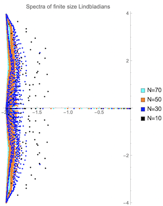
Figure 2: Spectrum of the Lindbladian corresponding to local dephasing (see (30)) restricted to $N=10,30,50,70$ lattice sites for $G=2$ where we have larger $N$ plotted first and they therefore appear behind smaller values of $N$. Notice how it seems that most of the spectrum converges to $-2+i[-4,4]$ as $N$ gets larger, but that we also see some spectrum in the interval $[-2,0]$.    

The model is given by choosing the Hamiltonian as nearest neighbour hopping

$$H=-\tilde{\Delta}=-\sum_{k\in\mathbb{Z}} {|{k}\rangle}{\langle{k+1}|} +{|{k+1}\rangle}{\langle{k}|}$$ (29)

and the local Lindblad operators as local dephasing, i.e. projectors onto single lattice sites $k\in\mathbb{Z}$

$$L_{k}=\outerproduct{k}{k}.$$ (30)

We notice that each Lindblad generator satisfies $L_{k}=L_{k}^{*}=L_{k}^{*}L_{k}=\outerproduct{k}{k}$. Now, define $Q$ by $Q=\sum_{k} L_{k}^{*}L_{k}=1\!\!1$ and therefore the model satisfies the assumptions of Theorem 3.8. Using Theorem 3.8, we can first determine the spectrum of the non-Hermitian part of the evolution $\mathcal{T}=\int_{ [0,2\pi]}^{\oplus} T(q)dq$ in Theorem 3.8 without the quantum jumps $\mathcal{F}=\int_{ [0,2\pi]}^{\oplus}F(q)dq$.

Proposition 5.1 (Spectrum of NHE local dephasing).

Let $H=-\Delta$ as in (29) and let the Lindblad operators $L_{k}$ be given as $\outerproduct{k}{k}$, then the generator of the non-Hermitian evolution $\mathcal{T}\in\mathcal{B}(\operatorname*{HS}(\ell^{2}(\mathbb{Z})))$ satisfies

$$\sigma(\mathcal{T})=-G+i[-4,4].$$

Proof.

Using Theorem 3.8 and $Q=\sum_{k} L_{k}^{*}L_{k}=1\!\!1$, we see that $T(q)$ is given by

$$T(q)=i(1-e^{-iq})S+i(1-e^{iq})S^{*}-G\;.$$ (31)

For fixed $q$ this corresponds to a tridiagonal Laurent operator with symbol curve $T(q,\theta)=i(1-e^{-iq})e^{i\theta}+i(1-e^{iq})e^{-i\theta}-G$. By Theorem 3.13 and Theorem 3.3, it follows that

$$\sigma(\mathcal{T})=\bigcup_{q\in[0,2\pi]}\sigma(T(q))=\bigcup_{q\in[0,2\pi]}\left\{T(q,\theta)\mid\theta\in[0,2\pi]\right\}.$$

Putting in the explicit form of the parameters from (31), we find

$$T(q,\theta)=-G+2i(\cos(\theta)-\cos(\theta-q))\,.$$

Since $\theta$ and $q$ can be varied independently over the interval $[-\pi,\pi]$ we can realize any value in $-G+i[-4,4]$ as claimed. ∎

From (31) we see that $\alpha(q)=i(1-e^{-iq}),\beta(q)=-G,\gamma(q)=i(1-e^{iq})$ are the entries of the tridiagonal matrix $T(q)$.

Remark 5.2 (Transfer matrix picture).

Notice that the proof of Proposition 5.1 is in some sense equivalent to finding out that the polynomial $\alpha x^{-1}+\beta+\gamma x$ has a root of absolute value 1 if and only if $z\in-G+[-4i,4i]$, where $\alpha,\beta,\gamma:[0,2\pi]\to\mathbb{C}$ are the diagonals of the tridiagonal matrix $T(q)$. This has an interpretation in terms of transfer matrices: If one considers the Laurent operator with $\alpha,\beta$ and $\gamma$ on the diagonal and solves it iteratively then a root of $\alpha x^{-1}+\beta+\gamma x$ of absolute value less than 1 corresponds to an exponentially decaying and therefore normalizable solution. Conversely, a root of absolute value strictly larger than 1 corresponds to an exponentially increasing and therefore not normalizable solution. In this picture, one can interpret the rank-one perturbation ${|{\Gamma_{R}}\rangle}{\langle{\Gamma_{L}}|}$ as boundary condition at $0$ for an iterative solution for positive and negative entries.

Thus, we have computed the spectrum of the non-Hermitian Hamiltonian. Turning now to the full Lindblad generator $\mathcal{L}$, we can characterize its spectrum depending on the dissipation strength by including the quantum jump part as a perturbation to the non-Hermitian part.

Proposition 5.3 (Full spectrum for local dephasing).

Let $H=-\tilde{\Delta}$ be the (modified) Laplacian defined in (29) and let the Lindblad operators $L_{k}$ be given as $\outerproduct{k}{k}$, then the Lindblad generator $\mathcal{L}$ satisfies

$$\sigma(\mathcal{L})=\left(-G+i[-4,4]\right)\cup\begin{cases}[-G,0],&\mbox{if }G\leq 4\\ [-G+\sqrt{G^{2}-16},0],&\mbox{otherwise}.\end{cases}\;.$$

Proof.

Since $T(q)$ is translation invariant its spectrum is essential. Thus, when $T(q)$ is compactly perturbed the spectrum can only be extended. So, as in the proof of Corollary 3.14, we get from Proposition 5.1 that

$$-G+[-4i,4i]=\sigma(\mathcal{T})\subset\sigma(\mathcal{L}).$$

The coefficients of the perturbation also follow from our consideration in Section 3. Based on Theorem 3.8, we find that $F(q)=G\outerproduct{0}{0}$, independent of $q$, which means that we may choose ${|{\Gamma_{L}}\rangle} ={|{\Gamma_{R}}\rangle}=\sqrt{G} {|{0}\rangle}$. Hence, both ${|{\Gamma_{L}}\rangle}$ and ${|{\Gamma_{R}}\rangle}$ are bounded vectors and $q\mapsto{\langle{0}|}(T(q)-z)^{-1}{|{0}\rangle}$ is continuous for $z\notin-G+[-4i,4i]$. Therefore, we may determine $\sigma(\mathcal{L})$ from Corollary  3.15 which leads to the condition

$$G{\langle{0}|}(T(q)- z)^{-1}{|{0}\rangle} =-1.$$ (32)

Thus, we now have to compute ${\langle{0}|}(T(q)-z)^{-1}{|{0}\rangle}$ which we elaborate on in Appendix A.7. Define $\lambda_{+}$ and $\lambda_{-}$ by (with a convention on taking square roots of complex numbers elaborated on in Appendix A.7 )

$$\lambda_{\pm} =-\frac{\beta}{2\gamma} \pm\sqrt{\left(\frac{\beta}{2\gamma}\right)^{2}-\frac{\alpha}{\gamma}}.$$ (33)

Let further, $\absolutevalue{\lambda_{2}}\leq\absolutevalue{\lambda_{1}}$ such that $\{\lambda_{1},\lambda_{2}\} =\{\lambda_{+},\lambda_{-}\}$. Then notice that the conditions of Lemma A.12 are satisfied and we may therefore $\absolutevalue{\lambda_{2}} <1< \absolutevalue{\lambda_{1}}$. Thus, we can use Lemma A.13 to find the inverse of the Laurent operator to obtain

$$-1=(-1)^{1\!\!1[\absolutevalue{\lambda_{-}} <1<\absolutevalue{\lambda_{+}} ]} \frac{G}{\sqrt{(\beta-z)^{2}-4\alpha\gamma }}.$$ (34)

Our strategy is to square the equation, solve to find a set of possible $z$ and then reinsert into (34) to see which sign is correct. The potential solutions satisfy

$$z=\beta\pm\sqrt{G^{2}+4\alpha\gamma}.$$

In the specific example with dephasing noise, we saw that $\beta=-G$, $\alpha=-ie^{-iq} +i$ and $\gamma=-ie^{iq}+i$. Thus, strictly speaking, the considerations above only apply when $q\neq 0$, in the case $q=0$ we see that $z=0$ is the only solution to (32).

As $\alpha\gamma=2(\cos(q)-1)$, we consider

$$z=-G\pm\sqrt{G^{2}+8(\cos(q)-1)}.$$

As $G^{2}+8(\cos(q)-1)\in[-16+G^{2},G^{2}]$ it is natural to consider the cases $G<4$ and $G\geq 4$.

In the case $G<4$ we have $-16+G^{2}<0$. Thus,

$$\bigcup_{q\in[0,2\pi]}\{\sqrt{G^{2}+8(\cos(q)-1)}\}=i[0,\sqrt{16-G^{2}}] \cup[0,G].$$

Therefore, the potential values of $z$ are

$$z\in[-G,0]\cup[-2G,-G]\cup\left(-G+i\left[-\sqrt{16-G^{2}},\sqrt{16-G^{2}}\right]\right).$$

Notice that since $\left[-\sqrt{16-G^{2}},\sqrt{16-G^{2}}\right]\subset[-4i,4i]$ this does not give additional spectrum.

It now remains to check the sign of the remaining possible solutions. From (34) we see that the square root must yield a (positive) real number and we at the same time need that $\absolutevalue{\lambda_{+}} <1<\absolutevalue{\lambda_{-}}$, so we only need to deal with the case where $0\leq G^{2}+8(\cos(q)-1)\leq G^{2}$. Then

$$\beta-z=\mp_{z}\sqrt{G^{2}+8(\cos(q)-1)}.$$

Using $\mp_{z}$ and $\mp_{\lambda}$ to denote two, on the outset, independent signs we obtain from (33) that

$$2\gamma\lambda_{\pm}=-(\beta-z)\pm_{\lambda}\sqrt{ \left(\beta-z\right)^{2}-4\alpha\gamma }=\pm_{z}\sqrt{G^{2}+8(\cos(q)-1)}\pm_{\lambda}\sqrt{ G^{2} }.$$

If $\pm_{z}=+$ then $\absolutevalue{\lambda_{-}} <\absolutevalue{\lambda_{+}}$ and $\pm_{z}=-$ then $\absolutevalue{\lambda_{+}} <\absolutevalue{\lambda_{-}}$. Thus, from (34) we see that $\pm_{z}=+$ is the only valid solution. Thus, only $z\in[-G,0]$ are valid solutions.

In the case $G\geq 4$: It holds that $-16+G^{2}\geq 0$ and therefore there is only one segment $[\sqrt{G^{2}-16},G]$. This observation translates into

$$z\in[-G+\sqrt{G^{2}-16},0]\cup[-2G,-G-\sqrt{G^{2}-16}].$$

Using a similar argument as above one finds that only the part $[-G+\sqrt{G^{2}-16},0]$ has the correct sign.

∎

We finish this subsection with the following remarks.

Emergence of two timescales: From Proposition 5.3 we see that if we change $G$ from a value below 4 to a value above 4 the spectrum transitions from being connected to consist of two connected components. Furthermore, increasing the dissipation strength $G$, the connected component of the spectrum containing $\{0\}$ shrinks. This indicates the emergence of two timescales in the dynamics. The first one corresponding to the fast decay at rate $e^{-tG}$ and a second one with a much slower decay. On the infinite lattice it is difficult to discuss the density of states, but it is noticed numerically in [22], that there are of the order of $L$ eigenvalues on the real axis close to $0$ and $L^{2}-L$ eigenvalues with real part close to $-G$. In general, such a phenomenon can be explained from symmetry as in [26, Appendix B.9].

Heuristic calculation of the finite-volume spectral gap:   In the dephasing case, that we study in section 5.1, it holds the solutions on the curve are given by

$$z=-G+\sqrt{G^{2}+8(\cos(q)-1)}.$$

Thus, naively we can let $q=\frac{2\pi}{N}$ and so $\cos(\frac{2\pi}{N})-1\approx\frac{1}{2}(\frac{2\pi}{N})^{2}=\frac{2\pi^{2}}{N^{2}}$ and thus as $\sqrt{1+x}\approx 1+\frac{x}{2}$ for small $x$ we obtain that

$$z\approx-G+\sqrt{G^{2}+8\frac{2\pi^{2}}{N^{2}}}\approx-G+G\left(1+\frac{16\pi^{2}}{G^{2}N^{2}} \right)=\frac{16\pi^{2}}{GN^{2}}.$$

This formula was also obtained in finite volume with periodic boundary conditions by Znidanic in [22, (8)].

5.2 Non-normal dissipators

Next, we turn to a model with non-normal Lindblad operators. The following family of dissipative models was studied in [70, 25, 71, 8]. For the Hamiltonian $H$ we still take the discrete Laplacian given in (29). The Lindblad operators are of the form

$$L_{k}=\left({|{k}\rangle} +e^{i\delta}{|{k+l}\rangle}\right)\left({\langle{k}|} -e^{-i\delta}{\langle{k+l}|}\right)$$ (35)

for some $\delta\in[0,2\pi]$ and $l\in\mathbb{N}$. Notice that $L_{k}$ is not normal. We have that

$$L_{k}^{*}L_{k}=2\outerproduct{k}{k} +2\outerproduct{k+l}{k+l} -2e^{i\delta} \outerproduct{k}{k+l}-2e^{-i\delta}\outerproduct{k+l}{k}.$$

Define $Q$ by

$$Q=\sum_{k\in\mathbb{Z}}L_{k}^{*}L_{k}=41\!\!1-2D_{l},$$

where $D_{l}$ is the operator which has $e^{i\delta}$ and $e^{-i\delta}$ on the $l$’th sub- and superdiagonal. To compute the form of the rank-one perturbation notice that all $\alpha_{r}$ from Theorem 3.8 are $0$ except for $\alpha_{0}=1,\alpha_{l}=e^{i\delta}$. Similarly, $\beta_{0}=1,\beta_{l}=-e^{-i\delta}$ and all other entries are 0.

Thus, from Theorem 3.8 we obtain

$$\frac{{|{\Gamma_{L}}\rangle}}{\sqrt{G}} =\sum_{r_{1},r_{2}} \alpha_{r_{1}} \overline{\alpha_{r_{2}}}e^{ir_{1}q}{|{r_{2}-r_{1}}\rangle}=(1+e^{ilq}){|{0}\rangle}+e^{i\delta}e^{ilq}{|{-l}\rangle} +e^{-i\delta}{|{l}\rangle}$$

as well as

$$\frac{{\langle{\Gamma_{R}}|}}{\sqrt{G}}=\sum_{r_{1}^{\prime},r_{2}^{\prime}} \beta_{r_{1}^{\prime}}e^{-ir_{1}^{\prime}q}\overline{\beta_{r_{2}^{\prime}}}{\langle{r_{2}^{\prime}-r_{1}^{\prime}}|}=(1+e^{-ilq}){\langle{0}|}-e^{-i\delta}e^{-ilq}{\langle{-l}|} -e^{i\delta}{\langle{l}|}.$$

We see that also the operator non-Hermitian evolution $T$ is given by

$$\left(-i\tilde{\Delta}-\frac{G}{2}Q\right)\otimes 1\!\!1+1\!\!1\otimes\left(i\tilde{\Delta}-\frac{G}{2}\overline{Q}\right)=\left(-i\tilde{\Delta}+GD_{l}\right)\otimes 1\!\!1+1\!\!1\otimes\left(i\tilde{\Delta}+G\overline{D_{l}}\right)-4G1\!\!1\otimes 1\!\!1$$

which is tridiagonal. Let us examine how this $Q$ transforms under the shift and Fourier transformation in the first variable that we do in Theorem 3.8. The term $-4G1\!\!1\otimes 1\!\!1$ is left invariant. The term $\left(iGD_{l}\right)\otimes 1\!\!1$ becomes:

$$Ge^{i\delta} e^{-ilq} \sum_{j} \outerproduct{j}{j-l}+Ge^{-i\delta}e^{iql} \sum_{j}\outerproduct{j}{j+l}.$$

For the term $1\!\!1\otimes\left(G\overline{D_{l}}\right)$ we get

$$Ge^{-i\delta} \sum_{j}\outerproduct{j}{j+l}+Ge^{i\delta} \sum_{j}\outerproduct{j}{j-l}.$$

In total,

$$T(q)=G\sum_{j}e^{-i\delta}\left( 1+e^{iql} \right)\outerproduct{j}{j+l}+e^{i\delta} \left(1+ e^{-ilq}\right)\outerproduct{j}{j-l}-4G1\!\!1\otimes 1\!\!1+i(1-e^{-iq})S+i(1-e^{iq})S^{*}.$$

We can see that the full operator has non-zero entries in 5 diagonals if $l>1$ so from now on we will assume that $l=1$ which is also the case mainly studied in [25] and [70]. In that case, we find the infinite band matrix with diagonals:

$$\alpha=i(1-e^{iq})+Ge^{-i\delta}\left(1+e^{iq}\right) \beta=-4G \gamma=i(1-e^{-iq})+Ge^{i\delta}\left(1+ e^{-iq}\right).$$

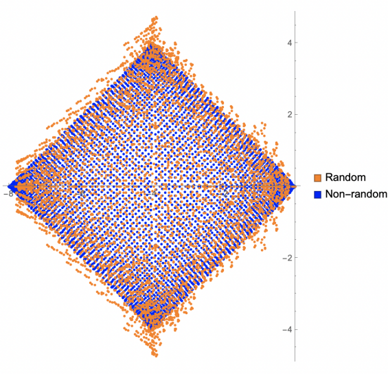
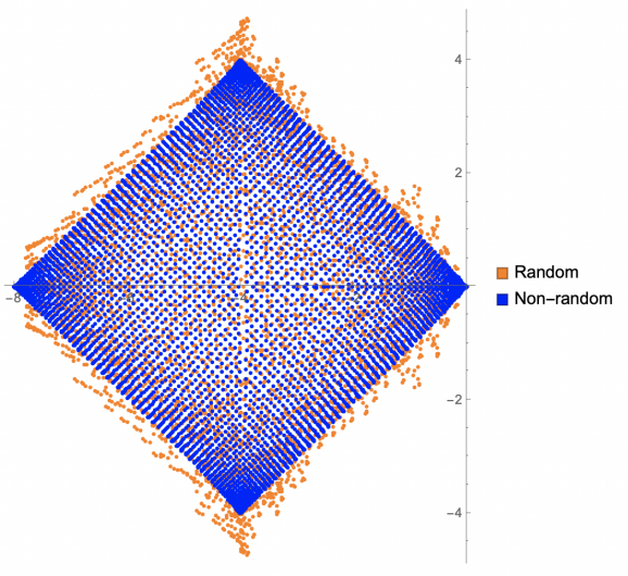
Figure 3: Spectrum $\mathcal{L}$ with non-normal Lindblad operators given by (35) with a random potential in orange and without in blue in the complex plane. In the right picture blue points are plotted on the top and on the left it is the orange points. In this case $G=1$, the lattice size $n=70$ and the support of the distribution of the strength of the external potential $V=2$. Notice how the blue points are ordered very regularly except that there is a vertical hole in the middle and those eigenvalues tend to collapse to the real axis. It seems that the main effect of the external field is to push the eigenvalues vertically.

Let us first determine the union of the $q$-wise spectra without the perturbation $F(q)$. See also Figure 4 for an illustration.

Proposition 5.4.

The spectrum of the non-Hermitian evolution for the Lindbladian from (35) in the case $l=1$ is given by

$$\sigma(\mathcal{T})=\bigcup_{q,\theta\in[0,2\pi]}\{-4G+2i\cos(\theta)-2i\cos(q-\theta)+2G\cos(\delta+\theta)+2G\cos(q-\delta-\theta)\}.$$

For $\delta=0$ and $\delta=\pi$ this set is the convex envelope of the points $-8G,-4i,0,4i$.

Proof.

As before, it holds by Corollary 3.14 and the fact that the spectrum of a Laurent operator is the image of the symbol curve that

$$\sigma(\mathcal{T})=\bigcup_{q\in[0,2\pi]}\sigma(T(q))=\bigcup_{q\in[0,2\pi]}\left\{ \delta(q)e^{-i\theta} +\beta+\gamma(q)e^{i\theta}\mid\theta\in[0,2\pi]\right\}.$$ (36)

The result now follows from a direct computation. For $\delta=0$ and $\delta=\pi$ it reduces to

$$\sigma(\mathcal{T}) =\bigcup_{q,\theta\in[0,2\pi]}\{-4G+\cos(\theta)\left(2i\pm 2G\right)+\cos(q-\theta)\left(-2i\pm 2G\right)\}$$

$$=\bigcup_{x,y\in[-2,2]}\{-4G+x\left(i\pm G\right)+y\left(-i\pm G\right)\}=\text{conv}(-8G,-4i,0,4i).$$

∎

Thus, we have proven that $\mathcal{T}$ is gapless even before adding the quantum jump term and therefore also afterwards when considering the full $\mathcal{L}$. We now turn to study the spectral effects of the perturbation.

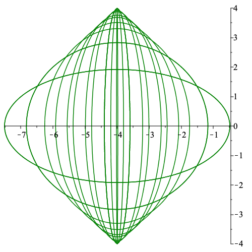
Figure 4: The ellipses corresponding to the spectrum of the Laurent matrices $T(q)$ in the model with non-normal Lindblad operators see for example (36). For the plot, we chose $\delta=0$ corresponding to Proposition 5.4. Notice how the union of the ellipses make up the quadrilateral described in Proposition 36, compare also to the shape in Figure 3.

Notice that for $\delta=0$ then $\alpha\gamma=2G^{2}\cos(q)+2G^{2}+2\cos(q)-2\in\mathbb{R}$. We now ask whether the set

$$\bigcup_{q\in[0,2\pi]}\left\{z\in\mathbb{C}\mid{\langle{\Gamma_{R}}|}(T(q)-z)^{-1}{|{\Gamma_{L}}\rangle} =-1\right\}$$

increases the spectrum. Absorbing $z$ into $\beta$ yields that $\beta=-4G-z$ and from Theorem 3.8 we find that ${|{\Gamma_{L}}\rangle}$ and ${\langle{\Gamma_{R}}|}$ have all entries zero except for the $-1,0,1$st entries, and that part of each of the vectors are

$${|{\Gamma_{L}}\rangle} =\sqrt{G} \begin{pmatrix}e^{iq}\\  1+e^{iq} \\ 1  \end{pmatrix}\text{ as well as } {\langle{\Gamma_{R}}|} =\sqrt{G}\begin{pmatrix}-1&1+e^{-iq} &-e^{-iq} \end{pmatrix},$$

in the basis $\{ {|{-1}\rangle},{|{0}\rangle},{|{1}\rangle}\}$ highlighting that we do allow for $q$-dependent ${|{\Gamma_{L}}\rangle}$ and ${\langle{\Gamma_{R}}|}$.

Now, let $\omega=\sqrt{ \beta^{2}-16\alpha\gamma}$ and then from Lemma A.13 the equation reduces to

$$-\frac{\omega}{G}=\frac{{\langle{\Gamma_{R}}|} T^{-1} {|{ \Gamma_{L}}\rangle}}{G} =\begin{pmatrix}-1&1+e^{-iq} &-e^{-iq} \end{pmatrix} \begin{pmatrix} 1&\frac{1}{\lambda_{1}}&\frac{1}{\lambda_{1}^{2}}\\  \lambda_{2}&1&\frac{1}{\lambda_{1}}\\  \lambda_{2}^{2}&\lambda_{2}&1\end{pmatrix}\begin{pmatrix}e^{iq}\\  1+e^{iq} \\ 1  \end{pmatrix}$$

$$=-e^{-iq}+2+2\cos(q)-e^{iq}+\lambda_{1}^{-1} (-1-e^{-iq}+e^{iq}+1)$$

$$-\lambda_{1}^{-2}+\lambda_{2}(1+e^{-iq}-1-e^{iq})-\lambda_{2}^{2}$$

$$=2+2\left(\frac{1}{\lambda_{1}}- \lambda_{2}\right)\sin(q)-\left(\frac{1}{\lambda_{1}^{2}}+\lambda_{2}^{2}\right),$$

where $\lambda_{1},\lambda_{2}$ are defined right after (33). This equation in $z$ can be numerically solved for fixed $q$ (and $G$). Numerical evidence suggests that the curve stays inside the quadrilateral $\operatorname*{conv}(-8G,-4i,0,4i)$ and therefore leads us to the following conjecture.

Conjecture 5.5.

For the Lindbladian $\mathcal{L}$ with Lindblad operators given by (35) and non-Hermitian evolution $A$ it holds that

$$\sigma(\mathcal{L})=\sigma(\mathcal{T})=\operatorname*{conv}(-8G,-4i,0,4i).$$

The reader can further compare with the plot of the spectrum in finite volume in Figure 3. Notice further, how Corollary 3.14 gives us the inclusion $\sigma(\mathcal{L})\supset\sigma(\mathcal{T})$. In particular, we obtain that $\mathcal{L}$ is gapless (independently of the conjecture). Interestingly, this gaplessness could be related to the dynamical behaviour in a random potential observed in [25]. A topic that we return to in Section 6.

5.3 Incoherent hopping

We now turn to an incoherent hopping studied numerically in [22]. Here, the Lindblad dissipators are hopping terms, they are given by $L_{k}={|{k}\rangle}{\langle{k+l}|}$. The numerical finding for finite sections with free boundary conditions of the lattice [22] is that the gap is uniformly positive as the length of the lattice increases. We find the spectrum for periodic boundary conditions.

Theorem 5.6.

Let $l\in\mathbb{Z}$. For the Lindbladian with $H=-\Delta$ and $L_{k}=\outerproduct{k}{k+l}$ it holds that

$$\sigma(\mathcal{L})=-G+i[-4,4]\cup\bigcup_{q\in[0,2\pi]}\left\{ -G\pm_{q}\sqrt{ e^{-2iql}G^{2}+8(\cos(q)-1)}\right\}$$

where $\pm_{q}$ is either $+$ or $-$ for each $q\in[0,2\pi]$.

Proof.

Notice that $L_{k}^{*}L_{k}=\outerproduct{k+l}{k+l}$ so still $Q=\sum_{k}L_{k}^{*}L_{k}=1\!\!1$. so $\left(-i\tilde{\Delta}-\frac{G}{2}Q\right)\otimes 1\!\!1+1\!\!1\otimes\left(i\tilde{\Delta}-\frac{G}{2}\overline{Q}\right)$ is tridiagonal with

$$\alpha=i(1-e^{iq}),\text{  }\beta=-G,\text{  }\gamma=i(1-e^{-iq})$$

on the diagonals. Furthermore,

$$F(q)=G\left(\sum_{r_{1},r_{2}} \alpha_{r_{1}} \overline{\alpha_{r_{2}}}e^{ir_{1}q}{|{r_{2}-r_{1}}\rangle} \right)\left(\sum_{r_{1}^{\prime},r_{2}^{\prime}} \beta_{r_{1}^{\prime}}e^{-ir_{1}^{\prime}q}\overline{\beta_{r_{2}^{\prime}}}{\langle{r_{2}^{\prime}-r_{1}^{\prime}}|}\right)$$

with $\alpha_{r}=\delta_{r,0}$ and $\beta_{r}=\delta_{r,1}$. Thus,

$${|{\Gamma_{L}}\rangle} =\sqrt{G}\sum_{r_{1},r_{2}} \alpha_{r_{1}} \overline{\alpha_{r_{2}}}e^{ir_{1}q}{|{r_{2}-r_{1}}\rangle} =\sqrt{G}{|{0}\rangle} \text{ and}$$

$${\langle{\Gamma_{R}}|} =\sqrt{G}\left(\sum_{r_{1}^{\prime},r_{2}^{\prime}} \beta_{r_{1}^{\prime}}e^{-ir_{1}^{\prime}q}\overline{\beta_{r_{2}^{\prime}}}{\langle{r_{2}^{\prime}-r_{1}^{\prime}}|}\right)=\sqrt{G}e^{-iql}{\langle{0}|}.$$

That means,

$${\langle{\Gamma_{R}}|}\frac{1}{T-z}{|{\Gamma_{L}}\rangle}=e^{-iql}G{\langle{0}|}\frac{1}{T-z}{|{0}\rangle}=\frac{(-1)^{1\!\!1[\absolutevalue{\lambda_{-}} <1<\absolutevalue{\lambda_{+}} ]}e^{-iql}G}{\sqrt{(\beta-z)^{2}-4\alpha\gamma}}.$$

So by Corollary 3.15 we need to solve

$$-1=(-1)^{1\!\!1[\absolutevalue{\lambda_{-}} <1<\absolutevalue{\lambda_{+}} ]}\frac{e^{-iql}G}{\sqrt{(\beta-z)^{2}-4\alpha\gamma}}.$$ (37)

Squaring yields

$$1=\frac{e^{-2iql}G^{2}}{(\beta-z)^{2}-4\alpha\gamma},$$

so solving for $z$ gives

$$z=\beta\pm\sqrt{ e^{-2iql}G^{2}+4\alpha\gamma} =-G\pm\sqrt{ e^{-2iql}G^{2}+8(\cos(q)-1)},$$

where we again, as in the proof of Proposition 5.3, have to throw some of the solutions away according to get the correct sign in (37). ∎

In Figure 5 and 6 we explicitly plot the solutions as a function of $q$ as well as the spectra obtained by exact diagonalization of $\mathcal{L}$ in finite volume. Notice how the predicted spectrum fits well with the numerical spectra for finite size systems only for the system with periodic boundary conditions, as is consistent with Theorem 4.5. This dramatic dependence on boundary conditions is sometimes called the non-Hermitian Skin effect [72, 73, 74]. It states that the spectra of non-Hermitian operators may exhibit dramatic dependence on boundary conditions. One could also view the difference between Toeplitz and Laurent operators this way. Furthermore, it is a feature of the non-Hermitian skin effect that the spectrum is pushed inwards and real eigenvalues start to appear [75]. This effect we also seen in Figure 5 and 6.

Figure 5: Exact diagonalization of the Lindbladian $\mathcal{L}$ in Section 5.3 for $l=1$, $G=1,2,5$ and $N=70$ comparison of the predicted curve with numerics with free boundary conditions. The red circle is the unit circle. Notice how the two curves do not match due to the non-Hermitian Skin effect.

Figure 6: Exact diagonalization of the Lindbladian in Section 5.3 for $l=1$, $G=1,2,5$ and $N=50$ comparison of the predicted curve with numerics with periodic boundary conditions. The red circle is the unit circle. Notice how the numerics and the analytical spectrum in the infinite volume fit.

5.4 Single particle sector of a quantum exclusion process

In a many-body setting a model with $L_{k}={|{k}\rangle}{\langle{k+1}|}$ and $L_{k}^{\prime}={|{k+1}\rangle}{\langle{k}|}$ was studied analytically in [76]. We briefly discuss how to adapt our methods to the single particle sector of that case and rederive the spectrum of the Lindbladian. Going through the proof of Theorem 3.8,  we see that we just get two independent contributions that diagonalize in the same way. Since we still use discrete Laplacian as the Hamiltonian, it holds that $\alpha=i(1-e^{iq})$ and $\gamma=i(1-e^{-iq})$ are unchanged. On the other hand, we get the sum $\sum_{k}L_{k}^{*}L_{k}=1\!\!1$ twice, which means that $\beta=-2G$. Therefore we have from Proposition 5.1 the spectrum of the non-Hermitian evolution $\sigma(\mathcal{T})=-2G+[-4i,4i]$.

We now turn to the spectrum of the full Lindbladian.

Theorem 5.7 (Hopping both ways).

If the system has Lindblad operators $L_{k}={|{k}\rangle}{\langle{k+1}|}$ and $L_{k}^{\prime}={|{k+1}\rangle}{\langle{k}|}$ then the spectrum is given by

$$\sigma(\mathcal{L})=[-2G,0]\cup\{-2G+i[-4,4]\}.$$

Proof.

We saw that the spectrum of the non-Hermitian evolution was given by $\sigma(\mathcal{T})=-2G+i[-4,4]$. Now, we calculate the spectrum of the quantum jump terms as follows:

$$F_{1}(q)=G\outerproduct{0}{0}e^{-iq}$$

$$F_{2}(q)=G\outerproduct{0}{0}e^{iq}.$$

Thus, in total the quantum jump contribution is

$$F(q)=F_{1}(q)+F_{2}(q)=2G\cos(q)\outerproduct{0}{0},$$

which is still rank-one and in contrast to the incoherent hopping discussed in Theorem 5.6 this expression is real. We use the same method to compute the spectrum as before

$$-1={\langle{\Gamma_{R}}|}\frac{1}{T-z}{|{\Gamma_{L}}\rangle}=\pm\frac{ 2\cos(q)G}{\sqrt{(\beta-z)^{2}-4\alpha\gamma}},$$

squaring and solving for $z$ and inserting $\alpha,\beta,\gamma$ yields that

$$z=-2G\pm\sqrt{ 4\cos^{2}(q)G^{2}+8(\cos(q)-1)}.$$

Let us analyze the function $f(q)=4\cos^{2}(q)G^{2}+8(\cos(q)-1)$. It has extremal points $q$ satisfying

$$0=8\cos(q)\sin(q)G^{2}+8\sin(q).$$

If $q\not\in\{0,\pi\}$ then

$$\cos(q)=-\frac{1}{G^{2}}$$

which has a solution if and only if $G\geq 1$.

This means that if $G<1$ then the only extremal points are at $q\in\{0,\pi\}$. The values are $f(0)=4G^{2}$ and $f(\pi)=4G^{2}-16$. Thus, by continuity and the intermediate value theorem, it holds that the range of $f$ is $[4G^{2}-16,4G^{2}]=[4G^{2}-16,0]\cup[0,4G^{2}]$. The first interval corresponds to the segments $\pm i[0,2\sqrt{4-G^{2}}]\subset i[-4,4]$. The second one to $[0,2G]$ analogously to the dephasing case from Section 5.1.

For $G\geq 1$ there is in addition the solution $\cos(q)=-\frac{1}{G^{2}}$ which has values $-\frac{4}{G^{2}}-8$. Since $G\geq 1$, the potential values of $f$ are extended to the interval $[-\frac{4}{G^{2}}-8,0]\cup[0,4G^{2}]$ which corresponds to solutions $i\left[-\sqrt{8+\frac{4}{G^{2}}},+\sqrt{8+\frac{4}{G^{2}}}\right]$ and $[0,2G]$ respectively. Still, since $G\geq 1$, it holds that $\sqrt{8+\frac{4}{G^{2}}} \leq 4$ and thus $i\left[-\sqrt{8+\frac{4}{G^{2}}},+\sqrt{8+\frac{4}{G^{2}}}\right]\subset i[-4,4]$. Thus, the spectrum is not extended in that case. ∎

6 Lindbladians with random potentials

In this section, we study models as in the previous section where we have added a random potential $V$ to the Hamiltonian $H$. The potential $V=\sum_{n\in\mathbb{Z}} V(n)\outerproduct{n}{n}$ is a random such that $(V(n))_{n\in\mathbb{Z}}$ is i.i.d. uniformly distributed potential in some range $[-\lambda,\lambda]$ for some $\lambda>0$. In the closed system case, the study of operators of that type was initiated in the celebrated work by Anderson [77] and has led to the field of random operator theory and the topic of Anderson localization.

Although, some results exist (e.g. [25, 9]), it is not clear what the effects of a random potential in an open quantum system are. In addition, there has recently been interest in random Lindblad systems from the point of view of random matrix theory [78, 27]. Our methods are however more along the lines of random operator theory [1]. Different methods that were also more random operator theoretic were pioneered in [9].

To study the spectrum of our random Lindbladians we use the following Lindbladian version of the Kunz–Soulliard Theorem from [79] generalised in [80]. We first need a bit of notation. Recall from Section 2 that we say that a (super)-operator $\mathcal{L}\in\mathcal{B}(\operatorname*{HS}(\mathcal{H}))$ is translationally covariant if for all $\rho\in\operatorname*{HS}(\mathcal{H})$

$$\mathcal{L}(S\rho S^{-1})=S^{-1} \mathcal{L}(\rho)S,$$

where $S$ is the translation with respect to the computational basis in $\operatorname*{HS}(\mathcal{H})$. In the examples without a random field, the Lindbladian is translation-invariant. We can separate the action of the potential by $\mathcal{E}_{V}$, where $\mathcal{E}_{V}(\rho)=-i[V,\rho]$.

We also need the numerical range of an operator $A$ which we define as follows:

$$W(A)=\{\langle v,Av\rangle\mid\norm{v}=1\}.$$

For example $W(\mathcal{E}_{V})=-i[\lambda,\lambda]$. The numerical range will be useful because its closure is an upper bound to the spectrum by the Toeplitz–Hausdorff Theorem [81, 82].

Theorem 6.1.

Let $\mathcal{L}_{0}$ be a translation-covariant operator on $\operatorname*{HS}(\mathcal{H})$, which satisfied that $\sigma_{\operatorname*{appt}}(\mathcal{L}_{0})=\sigma(\mathcal{L}_{0})$, (as ensured for our models of interest in Theorem 4.1). Let further $\{V(n)\}_{n\in\mathbb{Z}}$ be the i.i.d. random potential from above. Define $\mathcal{L}=\mathcal{L}_{0}+\mathcal{E}_{V}$ which is also an operator on $\operatorname*{HS}(\mathcal{H})$. Then almost surely it holds that

$$\sigma(\mathcal{L}_{0})\subset\sigma(\mathcal{L})\subset\overline{W(\mathcal{L}_{0})+W(\mathcal{E}_{V})},$$

where the second inclusion holds surely.

Proof.

Notice first that by the Toeplitz–Hausdorff Theorem [81, 82] it holds that

$$\sigma(\mathcal{L})\subset\overline{W(\mathcal{L})}\subset\overline{W(\mathcal{L}_{0})+W(\mathcal{E}_{V})}.$$

For the first inclusion, consider $\lambda\in\sigma_{\operatorname*{appt}}(\mathcal{L}_{0})$ and let $\{\rho_{n}\}_{n\in\mathbb{N}}$ be a Weyl sequence corresponding to $\lambda$ for $\mathcal{L}_{0}$. Without loss of generality assume that each $\rho_{n}$ is compactly supported in the sense that in the computational basis, we have that $\rho_{n}(x,y)=0$ for $(x,y)\not\in\Lambda_{R_{n}}\subset\mathbb{Z}^{2}$ for some large but finite box $\Lambda_{R_{n}}\subset\mathbb{Z}^{2}$. Then define

$$\Omega_{n}=\left\{\text{ for some }j_{n}\in\mathbb{Z}:\sup_{(x,y)\in\text{supp}(\rho_{n})}\absolutevalue{(-i)(V(x+j_{n})-V(y+j_{n}))}\leq\frac{1}{n}\right\},$$

and notice that each $\Omega_{n}$ is a set of full measure (one way to see this is that for any $k \in\mathbb{N}$ there is almost surely an $a\in\mathbb{Z}$ such that $\absolutevalue{V(a+j)}\leq\frac{1}{2n}$ for any $j\in\{1,\dots,k \}$). Hence $\Omega_{0}=\cap_{n\in\mathbb{N}}\Omega_{n}$ must have probability 1 as well. Thus, we can almost surely for each $n\in\mathbb{N}$ find integers $j_{n}\in\mathbb{Z}$ such that $\absolutevalue{(-i)(V(x+j_{n})-V(y+j_{n}))}\leq\frac{1}{n}.$

Now, define the sequence $\{\gamma_{n}\}_{n\in\mathbb{N}}\subset\operatorname*{HS}(\mathcal{H})$ by $\gamma_{n}=\rho_{n}(\cdot-j_{n})$, where $\rho_{n}(\cdot-j_{n})\in\operatorname*{HS}(\mathcal{H})$ is defined by ${\langle{x}|},\rho_{n}(\cdot-j_{n}){|{y}\rangle}=\rho_{n}(x-j_{n},y-j_{n})$, e.g. $\rho_{n}(\cdot-j_{n})$ is the operator $\rho_{n}$ shifted by $j_{n}$ in both coordinates.

Then $\{\gamma_{n}\}$ is a Weyl sequence for the eigenvalue $\lambda$ since by translation covariance of $\mathcal{L}_{0}$ it holds that

$$\left|\left|\left(\mathcal{L}-\lambda\right)(\gamma_{n})\right|\right|\leq\left|\left|\left(\mathcal{L}_{0}-\lambda\right)(\rho_{n})\right|\right|+\left|\left|\mathcal{E}_{V}(\gamma_{n})\right|\right|.$$

The first term is small since $\rho_{n}$ is a Weyl sequence for $\mathcal{L}_{0}$. For the second term, we estimate:

$$\left|\left|\mathcal{E}_{V}\left(\rho_{n}(\cdot-j_{n})\right)\right|\right| =\left|\left|\mathcal{E}_{V}\left(\sum_{x,y\in\operatorname*{supp}\rho_{n}+j_{n}}\rho_{n}(x-j_{n},y-j_{n}){|{x}\rangle}{\langle{y}|}\right)\right|\right|$$

$$=\left|\left|\sum_{x,y\in\operatorname*{supp}\rho_{n}+j_{n}}((-i)(V(x)-V(y))))\rho_{n}(x-j_{n},y-j_{n}){|{x}\rangle}{\langle{y}|}\right|\right|$$

$$=\left|\left|\sum_{x,y\in\operatorname*{supp}\rho_{n}}((-i)(V(x+j_{n})-V(y+j_{n}))))\rho_{n}(x,y){|{x+j_{n}}\rangle}{\langle{y+j_{n}}|}\right|\right|.$$

Now, if $\absolutevalue{(-i)(V(x+j_{n})-V(y+j_{n}))}\leq\frac{1}{n}$ for each $(x,y)\in\text{supp}(\rho_{n})$ then by definition of the Hilbert Schmidt inner product it holds that

$$\left|\left|\sum_{x,y\in\operatorname*{supp}\rho_{n}}((-i)(V(x+j_{n})-V(y+j_{n})))\rho_{n}(x,y){|{x+j_{n}}\rangle}{\langle{y+j_{n}}|}\right|\right|^{2}$$

$$=\sum_{x,y\in\operatorname*{supp}\rho_{n}}\absolutevalue{((-i)(V(x+j_{n})-V(y+j_{n}))))\rho_{n}(x,y)}^{2}$$

$$\leq\frac{1}{n^{2}}\sum_{x,y\in\operatorname*{supp}\rho_{n}}\absolutevalue{\rho_{n}(x,y)}^{2} \leq\frac{1}{n^{2}}.$$

It follows that $\left|\left|\mathcal{E}_{V}\left(\rho_{n}(\cdot-j_{n})\right)\right|\right|\leq\frac{1}{n}$ upon such a choice of $j_{n}$, which finished the proof.

∎

In the following sections, we will see how both of the two inclusions in Theorem 6.1 are in general strict.

Furthermore, one can see in Figure 3 how it seems as if the random field generally pushes eigenvalues vertically as would be the straightforward generalization of the theorem by Kunz and Soulliard [79]. However, the effect is much stronger in the bulk of the spectrum, whereas close to $\{0\}$ it does not seem as if the spectrum changes. A model that describes this phenomenon which is exactly solvable (even without the theory we have developed) is the following.

6.1 Exactly solvable model with random potential

Define on the Hilbert space $\ell^{2}(\mathbb{Z})$ the Lindbladian by $H=0$ and Lindblad operators $L_{k}={|{k}\rangle}{\langle{k}|}$. Then for any $i,j\in\mathbb{Z}$ we have that

$$\mathcal{L}_{0}({|{i}\rangle}{\langle{j}|})=G\sum_{k}{|{k}\rangle}{\langle{k}|}{|{i}\rangle}{\langle{j}|}{|{k}\rangle}{\langle{k}|}-\frac{1}{2} \{{|{k}\rangle}{\langle{k}|},{|{i}\rangle}{\langle{j}|}\}=G\left({|{i}\rangle}{\langle{i}|} \delta_{i,j}-{|{i}\rangle}{\langle{j}|}\right).$$

This means that all states of the form ${|{i}\rangle}{\langle{j}|}$ are eigenvalues with eigenvalue $-G$ if $i\neq j$ and $0$ if $i=j$. In particular, all states of the form ${|{i}\rangle}{\langle{i}|}$ for $i\in\mathbb{Z}$ are steady states. We conclude that $\sigma\left(\mathcal{L}_{0}\right)=\{0,-G\}$. Notice that in this case, we do have trace-class steady states in infinite volume.

To use the Lindblad analogue of Kunz–Soulliard we first need to consider the numerical range of $\mathcal{L}_{0}$. However, $\mathcal{L}_{0}$ is normal (indeed self-adjoint). That means that the numerical range is the convex hull of the spectrum i.e. $[-G,0]$.

We can find the exact spectrum of the model in a random potential by noticing that

$$\mathcal{L}(\outerproduct{i}{i})=0+\mathcal{E}_{V}(\outerproduct{i}{i})=(V(i)-V(i))\outerproduct{i}{i}=0$$

as well as

$$\mathcal{L}({|{i}\rangle}{\langle{j}|})=-G\outerproduct{i}{j} +\mathcal{E}_{V}(\outerproduct{i}{j})=-G\outerproduct{i}{j}+i(V(i)-V(j))\outerproduct{i}{j}.$$

Hence the spectrum $\sigma\left(\mathcal{L}\right)=\{-G+\lambda i[-1,1]\}\cup\{0\}$. Notice, how this is an example where both inclusions in Theorem 6.1 are strict. In the case at hand we can see that this happens because $\mathcal{L}$ leaves both the diagonal and off-diagonal subspaces of $\operatorname*{HS}(\ell^{2}(\mathbb{Z}))\cong\ell^{2}(\mathbb{Z}^{2})$ invariant. The potential $\mathcal{E}_{V}$ is zero on the diagonal part and therefore only the spectrum of the off-diagonal can be extended by $V$.

In the case of $H=-\Delta$ the two subspaces get mixed, the effects are more complicated and rigorous guarantees are harder to obtain. This is the aim of the next section.

6.2 Improving the upper bound on the spectrum

In the following, we prove an upper bound for the Anderson model with local dephasing. The model recently attracted attention in [83, 84]. In the following, we use the model to exemplify how we can use a new method to prove a non-trivial upper bound to the spectrum using the numerical range.

Theorem 6.2.

Consider the Anderson model $H=-\tilde{\Delta}+V$ with local dephasing defined in (30). Then for any $\rho\in\operatorname*{HS}(\mathcal{H})$ with $\norm{\rho}_{2}=1$ such that

$$\sum_{x\in\mathbb{Z}}\absolutevalue{\rho(x,x)}^{2}=a\in[0,1]$$

it holds that

$$\langle\rho,\mathcal{L}\rho\rangle\in Ga+\langle\rho,\mathcal{E}_{V}\rho\rangle+\langle\rho,\mathcal{T}\rho\rangle\in G(a-1)+i[f(a,\lambda),f(a,\lambda)]$$

with $f$ defined by $f(a,L)=4\left(1-a+ 2\sqrt{a} \sqrt{1-a}\right)+(1-a)\lambda$. It follows that

$$\sigma(\mathcal{L})\subset\bigcup_{a\in[0,1]}\left(G(a-1)+i[f(a,\lambda),f(a,\lambda)]\right).$$

We have plotted the upper bound to the spectrum in Figure 7.

Proof.

We first rewrite $\mathcal{L}$ using Theorem 3.8.

$$\mathcal{L}=\mathcal{L}_{0}+\mathcal{E}_{V}=\int_{[0,2\pi]}^{\oplus} T(q)dq+\int_{[0,2\pi]}^{\oplus} F(q)dq+\mathcal{E}_{V}=\mathcal{T} +\mathcal{F}+\mathcal{E}_{V}.$$

Again, we want to use the upper bound to the spectrum given the numerical range $\sigma(\mathcal{L})\subset\overline{W(\mathcal{L})}$, so we try to bound the numerical range of each term. So let $\rho\in\operatorname*{HS}(\mathcal{H})$ with $\norm{\rho}_{2}=1$. Notice first how that identity looks in our two pictures: Define ${|{\rho(q)}\rangle}=(\mathcal{F}_{1}\circ C\circ\operatorname*{vec}(\rho))(q)\in\ell^{2}(\mathbb{Z})$ Since $(\mathcal{F}_{1}\circ C\circ\operatorname*{vec}(\rho))$ is an isometric isomorphism it follows that

$$1=\norm{\rho}_{2}^{2}=\sum_{x,y\in\mathbb{Z}}\absolutevalue{\rho(x,y)}^{2}=\sum_{n\in\mathbb{Z}} \int_{0}^{2\pi}\absolutevalue{\langle\rho(q){|{n}\rangle}}^{2}dq.$$

Explicit calculation yields that

$${|{\rho(q)}\rangle}=\frac{1}{\sqrt{2\pi}}\sum_{x,y\in\mathbb{Z}}\rho(x,y)e^{-iqx} {|{y-x}\rangle},$$

which again means that

$$\langle 0{|{\rho(q)}\rangle}=\sum_{x \in\mathbb{Z}}\rho(x,x)e^{-iqx}.$$

So it follows that

$$\int_{0}^{2\pi}\absolutevalue{\langle\rho(q){|{0}\rangle}}^{2}dq=\sum_{x\in\mathbb{Z}}\absolutevalue{\rho(x,x)}^{2}=a,$$

where $a\in[0,1]$ is a real number that indicates how classical $\rho$ is. Notice that then $\sum_{x,y\mid x\neq y} \absolutevalue{\rho(x,y)}^{2}=1-a$. Now, we go term by term. For the first term, we estimate

$$\langle\rho,\mathcal{E}_{V}\rho\rangle =\Tr\left(\sum_{x,x^{\prime},y,y^{\prime}\in\mathbb{Z}} \overline{\rho(x^{\prime},y^{\prime})}{|{x^{\prime}}\rangle}{\langle{y^{\prime}}|} i(V(x)-V(y))\rho(x,y){|{x}\rangle}{\langle{y}|}\right)$$

$$=i\sum_{x,y\mid x\neq y} \absolutevalue{\rho(x,y)}^{2}(V(x)-V(y))\in i[-(1-a)\lambda,(1-a)\lambda]$$

since $V$ is supported in $[0,\lambda]$. Notice that the more classical a state is the less it is affected by an external field.

For the $T(q)$ term we know from (31) in the proof of Proposition 5.1 that $T(q)$ is tridiagonal with $\alpha,\beta,\gamma$ on the diagonals such that $\overline{\alpha(q)}=-\gamma(q)$ and that $\beta(q)=\beta$ is constant. Then

$$\langle\rho,\mathcal{T}dq\rho\rangle=\langle\rho,\int_{[0,2\pi]}^{\oplus} T(q)dq\rho\rangle =\int_{0}^{2\pi} \langle\rho(q),T(q)\rho(q)\rangle dq$$

$$=\sum_{n\in\mathbb{Z}} \int_{0}^{2\pi} \langle\rho(q){|{n}\rangle}(\alpha(q)\langle n+1{|{\rho(q)}\rangle}$$

$$+ \beta(q)\langle n{|{\rho(q)}\rangle}+\gamma(q){\langle{n-1}|}\rho(q)\rangle)dq$$

$$=\beta(q)\sum_{n\in\mathbb{Z}} \int_{0}^{2\pi} \absolutevalue{\langle n{|{\rho(q)}\rangle}}^{2}dq$$

$$+\sum_{n\in\mathbb{Z}} 2i\int_{0}^{2\pi}\text{Im}\left(\gamma(q)\langle\rho(q){|{n}\rangle}{\langle{n-1}|}\rho(q)\rangle\right)dq$$

$$=\beta(q)+\sum_{n\in\mathbb{Z}} 2i\int_{0}^{2\pi}\text{Im}\left(\gamma(q)\langle\rho(q){|{n}\rangle}{\langle{n-1}|}\rho(q)\right)dq.$$

We want to bound the second term. Define the sequence $l_{q,n}=\langle\rho(q){|{n}\rangle}$. And let $l_{q,n}^{\geq j}=l_{q,n}1\!\!1_{n\geq j}$ and similarly with $l_{q,n}^{\leq j}$. Using Cauchy–Schwarz in a few different spaces we obtain

$$\absolutevalue{\sum_{n\in\mathbb{Z}} \int_{0}^{2\pi}\text{Im}\left(\gamma(q)l_{q,n}\overline{l_{q,n-1}} \right)dq} \leq\norm{\gamma}_{\infty}\int_{0}^{2\pi}\absolutevalue{\sum_{n\in\mathbb{Z}} l_{q,n}\overline{l_{q,n-1}}} dq$$

$$\leq\norm{\gamma}_{\infty}\int_{0}^{2\pi}\absolutevalue{\sum_{n\leq-1}l_{q,n}\overline{l_{q,n-1}}}+\absolutevalue{\sum_{n\geq 2} l_{q,n}\overline{l_{q,n-1}}}$$

$$+ \absolutevalue{l_{q,0}\overline{l_{q,-1}}}+\absolutevalue{l_{q,1}\overline{l_{q,0}}} dq$$

$$\leq\norm{\gamma}_{\infty}\int_{0}^{2\pi}\norm{l_{q}^{\leq-1}}_{2}\norm{l_{q}^{\leq-2}}_{2}+\norm{l_{q}^{\geq 1}}_{2}\norm{l_{q}^{\geq 2}}_{2}+ \absolutevalue{l_{q,0}\overline{l_{q,-1}}}+\absolutevalue{l_{q,1}\overline{l_{q,0}}} dq$$

$$\leq\norm{\gamma}_{\infty}\left(1-a+ \sqrt{\int_{0}^{2\pi}\absolutevalue{ \langle\rho(q){|{0}\rangle}}^{2}dq} (\norm{l_{q,-1}}_{2}+\norm{ l_{q,1}}_{2})\right)$$

$$\leq\norm{\gamma}_{\infty}\left(1-a+ 2\sqrt{a} \sqrt{1-a}\right).$$

Notice that in particular, this vanishes as $a\to 1$, i.e. for classical $\rho$. Notice also that in our case of interest $\beta(q)=-G$ and $\norm{\gamma}_{\infty}=2$ yielding the second part of the bound.

For the $F(q)={|{\Gamma_{L}}\rangle}{\langle{\Gamma_{R}}|}$ we obtain

$$\langle\rho,\int_{[0,2\pi]}^{\oplus} {|{\Gamma_{L}}\rangle}{\langle{\Gamma_{R}}|}dq\rho\rangle=\int_{0}^{2\pi} \langle\rho(q){|{\Gamma_{L}}\rangle}\langle\Gamma_{R}{|{\rho(q)}\rangle}dq.$$

Thus, in the case where ${|{\Gamma_{L}}\rangle}{\langle{\Gamma_{R}}|}=G{|{0}\rangle}{\langle{0}|}$ in which case the term becomes

$$G\int_{0}^{2\pi}\absolutevalue{\langle\rho(q){|{0}\rangle}}^{2}dq=G\sum_{x\in\mathbb{Z}}\absolutevalue{\rho(x,x)}^{2}=Ga.$$

∎

Notice that $\real(\langle\rho,\mathcal{L}\rho\rangle)=G(a-1)=\real(\langle\rho,\mathcal{L}_{0}\rho\rangle)$. This means that the states as seen from the numerical range get more classical closer to $0$. This also implies the absence of a non-classical eigenvalue since one would then be able to find it in the numerical range. Thus, for the dephasing model, we see that the long-lived states are the classical even in the presence of an external (random) potential. In other words, the states that survive longest are very diagonal so we see very explicitly how the dephasing noise suppresses coherences something which was also noted for a simpler model in Chapter 8 of [85].

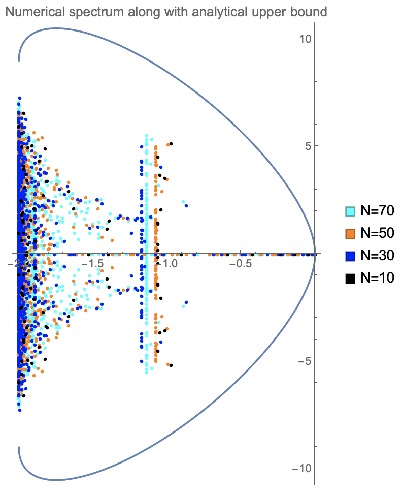
Figure 7: The numerical spectrum of the dephasing Lindbladian $\mathcal{L}$ in a random potential studied in Section 6.2  for $N\in\{10,30,50,70\},G=2,V=5$ along with the analytically calculated upper bound for the numerical range (and therefore the spectrum) sketched. Notice the line with real part close to $-1$ which is consistent with, but not predicted by our analysis. Notice further how it seems that the spectrum does not extend much when the real part is less than 1.

6.3 Further discussion of spectral effects of random potentials

Spectra of random Lindbladians have been studied in random matrix theory approaches in for example [78]. There a lemon-like shape of the spectrum was found. This shape is reminiscent of the spectrum in both Figure 3 and Figure 7 where there seems to be a tendency that the spectrum close to 0 extends less in the direction of the imaginary axis. This is also mimicked in the exactly solvable example in Section 6.1 and the discussion in the previous section. Furthermore, inspecting the non-random spectrum with and without the perturbation one can see how there is a similar phenomenon with eigenvalues jumping from the bulk of the non-Hermitian spectrum and down to the real line [22]. An analytical explanation stemming from the symmetries of the Lindbladian is given in [26]. The one also sees in a corresponding RMT model [28] and the previous example indicates a mechanism for this behaviour.

7 Discussion and further questions

We believe that the methods developed here can be applied to many one-particle open quantum systems of Lindblad form. In particular, we believe that many of our results generalize to $\mathbb{Z}^{d}$ for $d\geq 1$. Further, directions for the study could be many-body systems – in fact the model with non-normal Lindblad operators we studied in Section 5.2  is already a candidate for many-body localization in the many-body setting [86]. A simple example where the number of particles is not fixed could be to have a Lindbladian where the particle number can only decrease. If the system starts with one excitation, such models are used to describe the transport of an excitation during photosynthesis [6]. This would be one way to study the dynamics of similar systems which are not as intimately related to the spectra of $\mathcal{L}$ as discussed in Section 2.2. Another approach could be through the transport in the steady state as is for example done for a non-random system in [87]. A system that is almost within our framework, where transport in the steady state is studied is discussed in [88].

We have also seen how the quantum-jump terms increase the number of real eigenvalues, this effect was also observed in [22]. We can now explain the phenomenon corresponding to our first example in that case. For finite-dimensional systems an explanation was given using symmetries of the Lindbladian in [26, Appendix B.9]. The proof there relies on some rather old results, so it would be of value to obtain a self-contained proof. Along this line of investigation, one could try to obtain results on the density of states. Since relatively many eigenvalues are confined to the real line the density of states will potentially be challenging to define.

Furthermore, we have seen how the spectrum for the finite size numerics in some cases matches the analytic results for all of $\mathbb{Z}$ fairly well. This we have given an explanation of in Theorem 4.5, but it still remains to give a proof of ([66, Conjecture 7.3]), both in general and in our cases of interest. As shown by the examples in Figures 5 and 6  it will be important in that regard to use periodic boundary conditions, as it is the case in the corresponding question for Laurent operators compared to Toeplitz operators in [89].

Another direction of investigation is to expand on the spectral theory of Lindblad operators in a random potential and possibly prove a stronger lower bound to Theorem 6.1. In the self-adjoint case the spectrum and dynamics of the Hamiltonian in infinite volume are related through the RAGE theorem [2, 3, 4] much closer related than what we can prove for $\mathcal{L}$. Such a relation is probably difficult to recover since the notion of continuous spectrum breaks down in the non-normal case. However, we can still define the point spectrum of $\mathcal{L}$ to be spectrum that corresponds to normalizable eigenvectors. In that case, we can ask, in analogy with the case of the Anderson model, whether for large enough strength of the random potential $\lambda$ it is the case that $\sigma(\mathcal{L})$ has only point spectrum, in the sense of exponentially decaying (normalizable) eigenfunctions.

Appendix A Appendix

In the appendix, we provide some of the technicalities that we have postponed from the main part for clarity.

A.1 Remarks on spectral independence of Lindblad operators

Let us make some further remarks on the spectrum of Lindblad operators as an operator on the different Schatten spaces $\mathcal{S}_{p}$. If an operator $A$ is bounded on all Schatten spaces consistently, i.e. $A\in\mathcal{B}(\mathcal{S}_{p})$ for all $1\leq p\leq\infty$. Then we say that $A$ satisfies spectral independence if for all $1\leq p,q\leq\infty$ it holds that

$$\sigma_{\mathcal{B}(\mathcal{S}_{p})}(A)=\sigma_{\mathcal{B}(\mathcal{S}_{q})}(A).$$

In words this means that the spectrum of $A$ is independent of which Banach algebra $\mathcal{B}(\mathcal{S}_{p})$. To show how involved the situation is we start with the following remark.

Remark A.1.

Consider the Lindbladian with $H=V$ for some onsite operator $V=\sum_{i}V(i){|{i}\rangle}{\langle{i}|}$ and the dissipative part is $0$. In that case $\mathcal{L}(\rho)=-i[V,\rho]$. It holds that $\mathcal{L}({|{i}\rangle}{\langle{j}|})=-i(V(i)-V(j))({|{i}\rangle}{\langle{j}|})$ for each $i,j\in\mathbb{N}$. Thus, from one point of view, $\mathcal{L}$ is a Schur multiplier with the matrix with $(i,j)$’th index $-i(V(i)-V(j))$. If $\sup_{i}\absolutevalue{V(i)} <\infty$ then the Schur multiplier with bounded coefficients. In [48] an example of a Schur multiplier with bounded coefficients, although not of this form, that does not map trace class operators to trace class operators is given.

However, the operator discussed in [48] is very far from having Lindblad form which is a much stronger condition. Therefore, we can ask under which assumptions, for example, locality of the Lindblad operators, that spectral independence holds.

Question A.2.

Suppose that $H=\sum_{i}h_{i}$ and such that $h_{i},L_{k}$ have range bounded uniformly by some constant. Is $\sigma_{S_{p}}(\mathcal{L})$ independent of $p$?

In particular, in the case $\mathcal{L}(\rho)=-i[V,\rho]$ where $V{|{x}\rangle}=V(x){|{x}\rangle}$ such that $\absolutevalue{V(x)}\leq 1$ is it the case that $\sigma_{S_{p}}(\mathcal{L})$ is independent of $p$?

In particular, we are concerned with the case $\mathcal{L}(\rho)=-i[H,\rho]$ where $H=-\Delta+V$ for some diagonal non-translation-invariant potential $V$ as an operator from $\mathcal{S}_{p}$ to $\mathcal{S}_{p}$ (i.e. $V$ could be a random potential, that we will study later). Here $\Delta$ is the discrete Laplacian (in Dirac notation elaborated on at the beginning of Section 3) defined by

$$H=-\Delta=-\sum_{k\in\mathbb{Z}}\outerproduct{k}{k+1} + \outerproduct{k+1}{k}-2\outerproduct{k}{k},$$ (38)

where ${|{k}\rangle}$ is the position eigenstate at site $k\in\mathbb{Z}$.

It is natural to conjecture that $\sigma_{\mathcal{S}_{p}}\left(\mathcal{L}\right)$ is independent of $p\in[1,\infty]$, but this is beyond our current methods. However, we do present some partial results.

Proposition A.3.

Suppose that $1\leq p\leq p^{\prime}\leq\infty$ are Hölder conjugates, $\frac{1}{p}+\frac{1}{p^{\prime}} =1$ and that $\mathcal{L}\in\mathcal{B}(\mathcal{S}_{p})$ and $\mathcal{L}\in\mathcal{B}(\mathcal{S}_{p^{\prime}})$. Then $\mathcal{L}\in\mathcal{B}(\mathcal{S}_{q})$ for all $p\leq q\leq p^{\prime}$ and it holds that

$$\sigma_{\mathcal{S}_{q}}(\mathcal{L})\subset\sigma_{\mathcal{S}_{p}}(\mathcal{L})\cup\sigma_{\mathcal{S}_{p^{\prime}}}(\mathcal{L}).$$

Proof.

The first claim follows directly from the non-commutative Riesz-Thorin theorem (Theorem 2.1). For the second claim notice that if $z\not\in\sigma_{\mathcal{S}_{p}}(\mathcal{L})\cap\sigma_{\mathcal{S}_{p^{\prime}}}(\mathcal{L})$ then $(\mathcal{L}-z)^{-1}$ is bounded both from $\mathcal{S}_{p}$ to $\mathcal{S}_{p}$ and from $\mathcal{S}_{p^{\prime}}$ to $\mathcal{S}_{p^{\prime}}$. Again, by the non-commutative Riesz-Thorin theorem this means that $(\mathcal{L}-z)^{-1}$ is bounded from $\mathcal{S}_{q}$ to $\mathcal{S}_{q}$ for all $q\in[p,p^{\prime}]$ and so $z\not\in\sigma_{\mathcal{S}_{q}}(\mathcal{L})$ and we are done by contraposition. ∎

In fact, we can say a bit more using the Lindblad form. Let us start with the following lemma proving that the spectrum is invariant under complex conjugation in our infinite volume setting.

Lemma A.4.

Suppose that $\mathcal{L}$ is of the Lindblad form (1) and that $(\mathcal{A}_{1})$ holds. Then for all $p\in[1,\infty]$ it holds that $\sigma_{\mathcal{S}_{p}}(\mathcal{L})$ is closed under complex conjugation

$$\sigma_{\mathcal{S}_{p}}(\mathcal{L})=\overline{\sigma_{\mathcal{S}_{p}}(\mathcal{L})}.$$

Proof.

Suppose first that $\lambda\in\sigma_{\operatorname*{appt},\mathcal{S}_{p}}(\mathcal{L})$ there exists a sequence $\{\rho_{n}\}_{n\in\mathbb{N}}\subset\mathcal{S}_{p}(\mathcal{H})$ where

$$\norm{(\mathcal{L}-\lambda)(\rho_{n})}_{p}\to 0.$$

Then consider the modified Weyl sequence $\{\rho_{n}^{*}\}_{n\in\mathbb{N}}$ which satisfies that $\norm{\rho_{n}^{*}}_{p}=\norm{\rho_{n}}_{p}=1.$ This is a Weyl sequence for $\bar{\lambda}$ since

$$\norm{(\mathcal{L}-\bar{\lambda})(\rho_{n}^{*})}_{p}=\norm{((\mathcal{L}-\lambda)(\rho_{n}))^{*}}_{p}=\norm{(\mathcal{L}-\lambda)(\rho_{n})}_{p}\to 0.$$

We conclude that $\bar{\lambda}\in\sigma_{\operatorname*{appt},\mathcal{S}_{p}}(\mathcal{L})\subset\sigma_{\mathcal{S}_{p}}(\mathcal{L})$.

Now, assume that $\lambda\not\in\sigma_{\operatorname*{appt},\mathcal{S}_{p}}(\mathcal{L})$. Let $p^{\prime}$ be the Hölder conjugate of $p$ and consider $\mathcal{L}^{\dagger}:\mathcal{S}_{p^{\prime}} \to\mathcal{S}_{p^{\prime}}$ be the Banach space adjoint of $\mathcal{L}:\mathcal{S}_{p} \to\mathcal{S}_{p}$. It holds that $\lambda\in\sigma_{\operatorname*{res},\mathcal{S}_{p}}(\mathcal{L})=\sigma_{p,\mathcal{S}_{p^{\prime}}}(\mathcal{L}^{\dagger})=\sigma_{p,\mathcal{S}_{p^{\prime}}}(\tilde{\mathcal{L}})$,where $\sigma_{p,\mathcal{S}_{p^{\prime}}}$ here denotes the point spectrum in the algebra $\mathcal{S}_{p^{\prime}}$. Thus, there exists an operator $X\in\mathcal{S}_{p^{\prime}}$ such that $\tilde{\mathcal{L}}(X)=\lambda X$ which implies that $\tilde{\mathcal{L}}(X^{*})=\tilde{\mathcal{L}}(X)^{*}=\bar{\lambda}X^{*}$ and thus $\bar{\lambda}\in\sigma_{p,\mathcal{S}_{p^{\prime}}}(\tilde{\mathcal{L}})=\sigma_{\operatorname*{res},\mathcal{S}_{p}}(\mathcal{L})\subset\sigma_{\mathcal{S}_{p}}(\mathcal{L})$ which means that $\bar{\lambda}\in\sigma_{\mathcal{S}_{p}}(\mathcal{L})$. ∎

Now, we collect the results in the following theorem using that $\mathcal{L}$ and $\tilde{\mathcal{L}}$ on $\mathcal{S}_{p}$ and $\mathcal{S}_{p^{\prime}}$ are (Banach)-adjoints.

Theorem A.5.

Suppose that $1\leq p\leq p^{\prime}\leq\infty$ are Hölder conjugates, $\frac{1}{p}+\frac{1}{p^{\prime}} =1$ and that $\mathcal{L}\in\mathcal{B}(\mathcal{S}_{p})$ and $\mathcal{L}\in\mathcal{B}(\mathcal{S}_{p^{\prime}})$. Then $\mathcal{L}\in\mathcal{B}(\mathcal{S}_{q})$ for all $p\leq q\leq p^{\prime}$ and it holds that

$$\sigma_{\mathcal{S}_{q}}(\mathcal{L})\subset\sigma_{\mathcal{S}_{p}}(\mathcal{L})\cup\sigma_{\mathcal{S}_{p^{\prime}}}(\mathcal{L})=\sigma_{\mathcal{S}_{p}}(\mathcal{L})\cup\sigma_{\mathcal{S}_{p}}(\tilde{\mathcal{L}}).$$

In obtaining Theorem A.5 we did not use Lemma A.4 and therefore we did not use the property $\mathcal{L}(\rho^{*})=\mathcal{L}(\rho)^{*}$. A way to improve the Theorem A.5 would be to settle the following question positively.

Question A.6.

Suppose that $\mathcal{L}$ is of the Lindblad form (1) and that $(\mathcal{A}_{1})$ holds. Is it then the case that

$$\overline{ \sigma_{\mathcal{S}_{p}}(\mathcal{L})}=\sigma_{\mathcal{S}_{p}}(\tilde{\mathcal{L}})\text{?}$$

In that case, (which we consider fairly natural since it is true in finite dimensions) we would then obtain that for any $1\leq p\leq q\leq 2$ $\sigma_{\mathcal{S}_{q}}(\mathcal{L})\subset\sigma_{\mathcal{S}_{p}}(\mathcal{L})$ as well as the reverse inclusion in the case $2\leq q\leq p\leq\infty$. In particular, it would hold that $\sigma_{\mathcal{S}_{2}}(\mathcal{L})\subset\sigma_{\mathcal{S}_{1}}(\mathcal{L})$ meaning that our lower bounds to $\sigma_{\mathcal{S}_{2}}(\mathcal{L})$ would be lower bounds to $\sigma_{\mathcal{S}_{1}}(\mathcal{L})$.

A.2 Proof of Lemma 2.2 

We prove that $\mathcal{L}\in\mathcal{B}(\mathcal{B}{(\mathcal{H})})$. It is easy to see that by $(\mathcal{A}_{1})$ the commutator and anti-commutator terms in the Lindbladian are bounded. Thus, we are left with the operator $\mathcal{J}$ defined by $\mathcal{J}(X)=\sum_{k}L_{k}XL_{k}^{*}$.

Let $N$ be the weak limit of $\sum_{k}L_{k}L_{k}^{*}$. By assumption $\norm{N}_{\infty}<\infty$. Since $\sum_{k}L_{k}L_{k}^{*}$ is also self-adjoint it follows by the spectral radius theorem for every ${|{x}\rangle}\in H$ that

$$\sum_{k}\norm{ L_{k}^{*}{|{x}\rangle} }^{2}=\sum_{k}{\langle{x}|} ,L_{k}L_{k}^{*}{|{x}\rangle} ={\langle{x}|} ,\sum_{k}L_{k}L_{k}^{*}{|{x}\rangle} \leq\norm{N}_{\infty}\norm{x}^{2}.$$

Then consider $X\in\mathcal{B}{(\mathcal{H})}$ with $X\geq 0$. Then $X=AA^{*}$ for some $A\in\mathcal{B}{(\mathcal{H})}$ and it holds that

$$\sum_{k}L_{k}XL_{k}^{*}=\sum_{k}L_{k}AA^{*}L_{k}^{*}$$

is a sum of positive operators and therefore positive. We bound the norm

$${\langle{x}|},\sum_{k}L_{k}AA^{*}L_{k}^{*}{|{x}\rangle} =\sum_{k}{\langle{x}|},L_{k}AA^{*}L_{k}^{*}{|{x}\rangle}=\sum_{k}\norm{A^{*}L_{k}^{*}{|{x}\rangle}}^{2} \leq\sum_{k}\norm{A^{*} }^{2} \norm{L_{k}^{*}{|{x}\rangle}}^{2}$$

$$\leq\norm{A^{*} }^{2}\norm{N}_{\infty}\norm{x}^{2}.$$

Again, by self-adjointness of $\sum_{k}L_{k}AA^{*}L_{k}^{*}$ the spectral radius theorem holds and therefore if the numerical range is bounded then so is the norm. We conclude that

$$\norm{ \sum_{k}L_{k}AA^{*}L_{k}^{*}} \leq\norm{A}^{2}\norm{N}_{\infty}.$$

Now, for any element $X\in\mathcal{B}{(\mathcal{H})}$ we write $X=P_{1}-P_{2}+iP_{3}-iP_{4}$ where $P_{1},P_{2},P_{3},P_{4}$ are all positive and satisfy $\norm{P_{i}}\leq\norm{X}$ for each $i=1,\dots,4$ (see [90, Theorem 11.2 and 9.4]). Then

$$\norm{\mathcal{J}(X)}\leq 4\norm{X}\norm{N}_{\infty},$$

where we also used the $C^{*}$-identity since we could write $P_{i}=A_{i}A_{i}^{*}$ and that it holds that

$$\norm{A_{i}}^{2}=\norm{A_{i}{A_{i}}^{*}}=\norm{P_{i}} \leq\norm{X}.$$

We conclude that $\mathcal{J}$ as an operator on $\mathcal{B}{(\mathcal{H})}$ has a norm bounded by $4\norm{N}_{\infty}$.

A.3 Measurability in the proof of Theorem 3.12 

In this appendix, we prove that for each fixed $n\in\mathbb{N}$ there exists a measurable choice of the vectors $q\mapsto v_{q,n}$ in the proof of Theorem 3.12. We do that with inspiration from [91] and let $\{a_{m}\}_{m\in \mathbb{N}}$ be a countable dense subset of $\mathcal{H}$ which does not contain $0$. Then define $b_{m}=\frac{a_{m}}{\norm{a_{m}}}$. Recall that $I_{n}$ is a set such that $\absolutevalue{I_{n}}>0$ with $\norm{(A(q)-\lambda)^{-1} } \geq n$. Now, consider the function $N:I_{n}\to\mathbb{N}$ defined by

$$N(q)=\min\left\{m\in\mathbb{N}\mid\norm{(A(q)-\lambda)^{-1}b_{m}}\geq\frac{n}{2}\right\}.$$

Notice that $N$ is well-defined since $(A(q)-\lambda)^{-1}$ is bounded and hence continuous and by density of $\{a_{m}\}_{m\in \mathbb{N}}$. We claim that $N$ is also $\mathcal{B}\left(I_{n}\right)\--\mathcal{P}(\mathbb{N})$ measurable, where $\mathcal{B}\left(I_{n}\right)$ is the Borel sigma-algebra on $I_{n}$. To see that, notice first that since $q\mapsto(A(q)-\lambda)^{-1}$ is measurable then also $q\mapsto\norm{(A(q)-\lambda)^{-1}b_{m}}$ will be measurable for each $m$. Thus, the set

$$\left\{ q\in I_{n}\mid\norm{(A(q)-\lambda)^{-1}b_{m}}\geq\frac{n}{2}\right\}$$

is measurable. Now, it holds that

$$N^{-1}(\{1,\dots,k\})=\bigcup_{m =1}^{k}\left\{q\in I\mid\norm{(A(q)-\lambda)^{-1}b_{m}}\geq\frac{n}{2}\right\}$$

and this is sufficient to prove measurability of $N$. Now, since any function from $(\mathbb{N},\mathcal{P}(\mathbb{N}))$ to any measure space is measurable and compositions of measurable functions are measurable it holds that $q\mapsto b_{N(q)}$ is measurable. We then pick $v_{q,n}=b_{N(q)}$.

A.4 Proof of Theorem 3.13 

Proof.

We use the characterisation from Theorem 3.12. Whenever $\lambda\not\in\sigma(A(q))$ define the resolvent $R(q)=(A(q)-\lambda)^{-1}$. Then if both $R(p),R(q)$ exist it follows from the resolvent equation that

$$\absolutevalue{ \norm{R(p)}-\norm{R(q)}}\leq\norm{R(p)} \norm{A(p)-A(q)} \norm{R(q)}.$$ (39)

”$\subset$”: We prove the following stronger assertion.

Claim A.7.

For any $p_{0}\in[0,2\pi]$ and $\varepsilon>0$ it holds that

$$\sigma_{\varepsilon}(A(p_{0}))\subset\bigcup_{p\in[0,2\pi]}^{\operatorname*{ess}}\sigma_{2\varepsilon}(A(p)).$$ (40)

Let us first prove the claim.

Proof of Claim.

To prove the claim, let $\lambda\in\sigma_{\varepsilon}(A(p_{0}))$.

Case 1: Suppose first that $\lambda\not\in\sigma(A(p_{0}))$. This means that $\frac{1}{\varepsilon}\leq\norm{ R(p_{0})}<\infty$. Suppose that $\norm{R(p_{0})} \leq K<\infty$. Assume for contradiction that there is a sequence $p_{n}\to p_{0}$ such that $\norm{R(p_{n})}\to\infty$. By continuity (cf. Lemma A.10) there exists a $\delta>0$ such that $\norm{A(p)-A(q)} \leq\frac{1}{2K}$ as long as $\absolutevalue{p-q} <\delta$. If we pick $N$ such that $\absolutevalue{p_{n}-p_{0}}<\delta$ for $n\geq N$ this means that

$$\absolutevalue{ \norm{R(p_{0})}-\norm{R(p_{n})}}\leq\norm{R(p_{0})} \norm{A(p_{0})-A(p_{n})} \norm{R(p_{n})}\leq\frac{\norm{R(p_{n})}}{2K}.$$

Thus, $\frac{\norm{R(p_{n})}}{2} \leq \norm{R(p_{0})}$ and hence $\norm{R(p_{0})}=\infty$ which is a contradiction. We conclude that there exists a $\gamma>0$ such that $\sup_{p:\absolutevalue{p-p_{0}}\leq\gamma} \norm{R(p)}\leq K_{2}<\infty$. Thus, the resolvent bound (39) ensures that there is an $\theta>0$ such that if $\absolutevalue{p-p_{0}}\leq\theta$ then $\norm{R(p)}\geq\frac{1}{2\varepsilon}$. This means that $\lambda\in\sigma_{2\varepsilon}(A(p))$ for all $p$ with $\absolutevalue{p-p_{0}}\leq\theta$. Again this implies that $\lambda\in\bigcup_{p\in[0,2\pi]}^{\operatorname*{ess}}\sigma_{2\varepsilon}(A(p))$, proving the claim in the case $\lambda\not\in\sigma(A(p_{0}))$.

Case 2:  Now, let $\lambda\in\sigma(A(p_{0}))\subset\sigma_{\varepsilon}(A(p_{0}))$. Absorb $\lambda$ into $A$ for ease of notation. Now, suppose that $(p_{n})_{n\in\mathbb{N}}$ is a sequence converging to $p_{0}$ and assume that $\norm{R(p_{n})}\leq C$ uniformly in $n$. Then

$$\absolutevalue{ \norm{R(p_{n})}-\norm{R(p_{m})}}\leq\norm{R(p_{n})} \norm{A(p_{n})-A(p_{m})} \norm{R(p_{m})}\leq C^{2}\norm{ A(p_{n})-A(p_{m})},$$

so the sequence $(R(p_{n}))_{n\in\mathbb{N}}$ is Cauchy and hence convergent to some $R_{0}$. It holds by norm continuity that

$$\norm{R(p_{n})A(p_{0})-1\!\!1} =\norm{R(p_{n})(A(p_{0})-A(p_{n}))} \leq\norm{R(p_{n})} \norm{A(p_{0})-A(p_{n})} \leq C \norm{A(p_{0})-A(p_{n})}\to 0.$$

Similarly,$\norm{A(p_{0})R(p_{n})-1\!\!1} \to 0$. Since further

$$\norm{R_{0}A(p_{0})-1\!\!1} \leq\norm{R(p_{n})A(p_{0})-1\!\!1} +\norm{R_{0}-R(p_{n})} \norm{A(p_{0})} \to 0,$$

we conclude that $R_{0}A(p_{0})=1\!\!1$ and similarly $A(p_{0})R_{0}=1\!\!1$. This contradicts that $A(p_{0})$ is invertible. So we conclude that no such sequence $p_{n}$ exists. Hence for our given $\varepsilon>0$ there is a $\delta>0$ such that $\norm{R(p)}\geq\frac{1}{\varepsilon}$ for every $p\in[p_{0}- \delta,p_{0}+\delta]$. This means that $\lambda\in\bigcup_{p\in[0,2\pi]}^{\operatorname*{ess}}\sigma_{2\varepsilon}(A(p))$. ∎

So we conclude that for all $\varepsilon>0$ it holds that

$$\sigma_{\varepsilon}(A(p_{0}))\subset\bigcup_{p\in[0,2\pi]}^{\operatorname*{ess}}\sigma_{2\varepsilon}(A(p))$$ (41)

and therefore by Theorem 3.12

$$\sigma(A(p_{0}))\subset\bigcap_{\varepsilon>0} \sigma_{\varepsilon}(A(p_{0}))\subset\bigcap_{\varepsilon>0}\bigcup_{p\in[0,2\pi]}^{\operatorname*{ess}}\sigma_{2\varepsilon}(A(p))=\sigma\left(\int^{\oplus}_{[0,2\pi]}A(p)dp\right)$$

Since this holds for any $p_{0}\in[0,2\pi]$ we have proven one inclusion.

”$\supset$”: For the converse let $\lambda\in\bigcap_{\varepsilon>0} \left(\bigcup^{\operatorname*{ess}}_{q\in I}\sigma_{\varepsilon}(A(q))\right)$. Suppose for contradiction that $\lambda\not\in\sigma(A(q))$ for any $q\in I$. It then follows from the resolvent bound (39) that the function $N:I\to\mathbb{R}$ defined by $N(q)=\norm{(A(q)-\lambda)^{-1}}$ is continuous. Now,

$$S_{n}=\left\{q\in I\mid\lambda\in\sigma_{\frac{1}{n}}(A(q)) \right\} =\left\{q\in I\mid\norm{ A(q)-\lambda)^{-1}}\geq n\right\} =N^{-1}\left([n,\infty)\right).$$

Since $N$ is continuous and $[n,\infty)$ is closed we must have that $S_{n}$ is closed. Further, we must have that $S_{n}\subset S_{n-1}$ and that $S_{n}$ is non-empty for each $n\in\mathbb{N}$. Thus, by the finite intersection property (since $I$ is compact) it holds that $\bigcap_{n\in\mathbb{N}}S_{n}$ is non-empty. So let $q_{0}\in S_{n}$ for each $n\in\mathbb{N}$. Then $\norm{(A(q_{0})-\lambda)^{-1}}\geq n$ for all $n\in\mathbb{N}$ and thus $\lambda\in\sigma(A(q_{0}))$ which is a contradiction. So we conclude that $\lambda\in\sigma(A(q))$ for at least one $q\in I$ and then $\lambda\in\bigcup_{q\in I}\sigma(A(q))$.

∎

A.5 Spectrum of rank-one perturbation of Laurent operators

In this appendix, we prove the following relation that was used in the proof of Corollary 3.15.

$$\sigma(T(q)+F(q))=\sigma(T(q))\cup\left\{\lambda\in\mathbb{C}\mid{\langle{\Gamma_{R}}|}(T(q)-\lambda)^{-1}{|{\Gamma_{L}}\rangle} =-1\right\}.$$

$"\supset:"$ From the proof of Corollary 3.14 we saw that $\sigma(T(q))\subset \sigma(T(q)+F(q))$. So let $\lambda\not\in\sigma(T(q))$ and ${\langle{\Gamma_{R}}|}(T(q)-\lambda)^{-1}{|{\Gamma_{L}}\rangle} =-1$. Assume for contradiction that $T(q)+F(q)-\lambda$ is invertible. Let for ease of notation $T=T(q)-\lambda$. Then the resolvent equation states that

$$\frac{1}{T+{|{\Gamma_{L}}\rangle}{\langle{\Gamma_{R}}|}} =\frac{1}{T}-\frac{1}{T+{|{\Gamma_{L}}\rangle}{\langle{\Gamma_{R}}|}}{|{\Gamma_{L}}\rangle}{\langle{\Gamma_{R}}|}\frac{1}{T}.$$ (42)

Suppose that ${\langle{\Gamma_{R}}|}\frac{1}{T}{|{\Gamma_{L}}\rangle}=-1$ then multiplying with ${|{\Gamma_{L}}\rangle}$ from the right yields that $T^{-1}{|{\Gamma_{L}}\rangle}=0$, which is a contradiction.

$"\subset:"$ Assume that $T$ is invertible and that ${\langle{\Gamma_{R}}|}\frac{1}{T}{|{\Gamma_{L}}\rangle} \neq-1$. It is then straightforward to check that the following operator is well defined and an inverse to $T+{|{\Gamma_{L}}\rangle}{\langle{\Gamma_{R}}|}$

$$\frac{1}{T} -\frac{1}{{\langle{\Gamma_{R}}|}\frac{1}{T}{|{\Gamma_{L}}\rangle} +1} \frac{1}{T}{|{\Gamma_{L}}\rangle}{\langle{\Gamma_{R}}|}\frac{1}{T},$$

so we conclude that $T+{|{\Gamma_{L}}\rangle}{\langle{\Gamma_{R}}|}$ is invertible.

A.6 Resolvent norm estimates

Proof of Lemma 4.11.

First,  $\sup_{z\in V} \norm{(T(q)-z)^{-1}}\leq C<\infty$ for some $C>0$ To see that let $z_{n}\in V$ be a sequence such that $\norm{(T(q)-z_{n})^{-1}}\to\infty$. Since $\bar{V}$ is compact then $z_{n}$ has a convergent subsequence and it holds that $z_{n}\to z_{0}$ with $\norm{(T(q)-z_{0})^{-1}}=\infty$, hence $z_{0}\in\sigma(T(q))$ which is a contradiction to the construction of $V$.

Second, we show $\sup_{z\in V,n\in\mathbb{N}} \norm{(T(q_{n})-z)^{-1} }\leq C<\infty$. We first need the following claim.

Claim A.8.

For any $z\in V$ then

$$\sup_{n\in\mathbb{N}} \norm{(T(q_{n})-z)^{-1} } <\infty$$

Proof.

Suppose for contradiction that

$$\sup_{n\in\mathbb{N}} \norm{(T(q_{n})-z)^{-1} } =\infty$$

Then for every $\varepsilon>0$, there is a $n$ large enough such that for a subsequence

$$z\in\sigma_{\varepsilon}(T(q_{n}))\subset\bigcup_{q\in[0,2\pi]}^{\operatorname*{ess}}\sigma_{2\varepsilon}(T(q)),$$

where the inclusion follows from (41). Thus,

$$z\in\bigcap_{\varepsilon>0}\bigcup_{q\in[0,2\pi]}^{\operatorname*{ess}}\sigma_{2\varepsilon}(T(q))=\bigcup_{q\in[0,2\pi]}\sigma(T(q)),$$

which is a contradiction. ∎

Claim A.9.

$\sup_{z\in V,n\in\mathbb{N}} \norm{(T(q_{n})-z)^{-1} }\leq C<\infty$

Proof.

Assume first for contradiction that $\sup_{z\in V,n\in\mathbb{N}} \norm{(T(q_{n})-z)^{-1} }=\infty$. Then find a subsequence $(q_{n},z_{n})$ such that $\norm{(T(q_{n})-z_{n})^{-1} }\to\infty$, by compactness of $\bar{V}$ and $[0,2\pi]$ a suitable subsubsequence converges to some point $(q_{0},z_{0})\in[0,2\pi]\times V$.

Assume now for contradiction that $\norm{(T(q_{0})-z_{0})^{-1}} <\infty$ For any $(q,z)\in[0,2\pi]\times V$ it follows by the resolvent equations that

$$\absolutevalue{\norm{(T(q_{0})-z_{0})^{-1}} -\norm{ (T(q)-z)^{-1}}} \leq\norm{(T(q_{0})-z_{0})^{-1} -(T(q)-z)^{-1}}$$

$$\leq\norm{(T(q_{0})-z_{0})^{-1} -(T(q)-z_{0})^{-1}} +\norm{(T(q)-z_{0})^{-1} -(T(q)-z)^{-1}}$$

$$\leq\norm{(T(q_{0})-z_{0})^{-1}}\norm{T(q_{0})-T(q)} \norm{ (T(q)-z_{0})^{-1}}$$

$$+\norm{(T(q)-z_{0})^{-1}}\absolutevalue{z-z_{0}} \norm{ (T(q)-z)^{-1}}$$

$$\leq C\norm{T(q_{0})-T(q)}+C\absolutevalue{z-z_{0}}  \norm{ (T(q)-z)^{-1}}.$$

Thus, for any $z$ such that $\absolutevalue{z-z_{0}}\leq\frac{1}{2C}$ then we conclude for any $q\in[0,2\pi]$ that

$$\norm{(T(q_{0})-z_{0})^{-1}} \geq\norm{(T(q)-z)^{-1}}-\absolutevalue{\norm{(T(q_{0})-z_{0})^{-1}} -\norm{(T(q)-z)^{-1}}}$$

$$\geq\norm{(T(q)-z)^{-1}}-C\norm{T(q_{0})-T(q)}-\frac{1}{2} \norm{ (T(q)-z)^{-1}}$$

$$=\frac{1}{2} \norm{(T(q)-z)^{-1}}-C\norm{T(q_{0})-T(q)}.$$

Thus, if $(q,z)\to(q_{0},z_{0})$ and $\norm{(T(q)-z)^{-1}}\to\infty$ then $\norm{(T(q_{0})-z_{0})^{-1}} = \infty$ which is a contradiction to $\norm{(T(q_{0})-z_{0})^{-1}} <\infty$ and so we conclude that $\norm{ (T(q_{0})-z_{0})^{-1}} = \infty$. That means that $z_{0}\in\sigma(T(q_{0}))$ since $z_{0}\in\bar{V}$ this contradicts the construction of $V$ and therefore $\sup_{z\in V,n\in\mathbb{N}} \norm{(T(q_{n})-z)^{-1} }=\infty$ and so the claim is proven. ∎

∎

For completeness, we write out the norm continuity of $q\mapsto T(q)$ in the case that is relevant to us.

Lemma A.10.

Let $r\in\mathbb{N}$ and $T(q)$ be an $r$-diagonal Laurent operator with smooth functions $a_{i}:[0,2\pi]\to\mathbb{C}$ on the $i$’th diagonal for $-r\leq i\leq r$. Then if $q \to q_{n}$ it holds that

$$\norm{T(q)-T(q_{n}}\to 0.$$

Proof.

The proof is a simple computation.

$$\norm{T(q_{n})-T(q)} =\norm{ \sum_{i=-r}^{r}(a_{i}(q)-a_{i}(q_{n}))S^{i}} \leq\sum_{i=-r}^{r}\absolutevalue{a_{i}(q)-a_{i}(q_{n})} \to 0$$

as $q\to q_{n}$ by continuity the functions $a_{i}$. ∎

A.7 Invertibility of bi-infinite tridiagonal Laurent matrices

In this appendix, we discuss the inversion of bi-infinite tridiagonal Laurent matrices.

In Corollary 3.15 we saw that we could find the spectrum of $\mathcal{L}$ which was not just the spectrum of the non-Hermitian evolution by finding solutions to the equation

$${\langle{\Gamma_{R}}|}(T(q)-\lambda)^{-1}{|{\Gamma_{L}}\rangle} =-1.$$

In our applications, $T(q)-\lambda$ is a tridiagonal Laurent operator and thus to find explicit expressions we need to evaluate matrix elements of the inverse of such a matrix. For a tridiagonal operator with $\alpha,\beta$ and $\gamma$ on the diagonal the symbol curve is given by

$$a(z)=\alpha z^{-1}+\beta+\gamma z,z\in\mathbb{T},$$

which is a (possibly degenerate) ellipse. Thus, the spectrum always forms a (possibly degenerate) ellipse in that case. In the cases where our Lindblad operators are supported on at most two lattice sites, by Theorem 3.8 the corresponding Laurent operator will be tridiagonal.

If the matrix has $\alpha(q),\beta(q),\gamma(q)$ on the diagonals it will be useful to study the following equation

$$\alpha+\beta x+\gamma x^{2}=0.$$ (43)

In particular, we would like to know whether the two solutions $\lambda_{1},\lambda_{2}$ to the equation satisfy that

$$\absolutevalue{\lambda_{1}} <1<\absolutevalue{\lambda_{2}}.$$

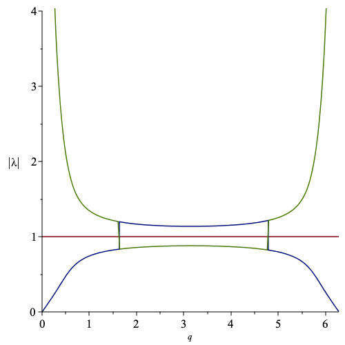
Figure 8: Plot of the absolute value of the two solutions to (43), for relevant parameters in the dephasing model for $G=1$ and $\lambda=-0.5+i$.

To define square roots we will use the following convention.

Convention A.11.

For a $z\in\mathbb{C}$ the two branches $\pm\sqrt{z}$ are defined such that $\real(+\sqrt{z})\geq 0$ and $\real(-\sqrt{z})\geq 0$. If $\real( +\sqrt{z})=0$ then we use the convention that $\imaginary(+\sqrt{z})\geq 0$.

The following lemma will be useful. We also sketch the situation in Figure 8.

Lemma A.12.

Let $\alpha,\beta,\gamma:S^{1}\to\mathbb{C}$ be continuous functions. Suppose that $T(q)$ is a family of tridiagonal Laurent matrices with $\alpha(q),\beta(q),\gamma(q)$ on the diagonals, which is invertible for all $q$. Assume further that $\gamma(q)=0$ for at most one $q$ and that there exists $q_{0},q_{1}$ such that

$$\absolutevalue{\alpha(q_{0})} \geq\absolutevalue{\gamma(q_{0})} \text{ and } \absolutevalue{\alpha(q_{1})} \leq\absolutevalue{\gamma(q_{1})}.$$

Let $\lambda_{1}(q),\lambda_{2}(q)$ be the two solutions of $\alpha(q)+\beta(q)x+\gamma(q)x^{2}=0$ such that $\absolutevalue{\lambda_{1}} \leq\absolutevalue{\lambda_{2}}$. Then for all $q$

$$\absolutevalue{\lambda_{2}(q)} <1<\absolutevalue{\lambda_{1}(q)}.$$

Proof.

For all $q$ such that $\gamma(q)\neq 0$ we can find the roots as

$$\lambda_{\pm} =-\frac{\beta}{2\gamma} \pm\sqrt{\left(\frac{\beta}{2\gamma}\right)^{2}-\frac{\alpha}{\gamma}},$$ (44)

where we used the convention. From Vieta’s formula, we also know that $\lambda_{+}\lambda_{-}=\frac{\alpha}{\gamma}$. Notice that since we have assumed that $T(q)$ is invertible we know that $\absolutevalue{\lambda_{+}}$ and $\absolutevalue{\lambda_{-}}$ are never equal to 1.

Thus, for at least one $q_{0}$ it holds that $\absolutevalue{\lambda_{+}\lambda_{-}}\geq 1$. That means either $\absolutevalue{\lambda_{1}(q_{0})} \geq\absolutevalue{\lambda_{2}(q_{0})}\geq 1$ or $\absolutevalue{\lambda_{1}(q_{0})} <1<\absolutevalue{\lambda_{2}(q_{0})}$. Similarly since for at least one $q_{1}$ it holds that $\absolutevalue{\lambda_{+}\lambda_{-}}\leq 1$ this means that either $\absolutevalue{\lambda_{1}(q_{1})} <1<\absolutevalue{\lambda_{2}(q_{1})}$ or $\absolutevalue{\lambda_{1}(q_{1})} \leq\absolutevalue{\lambda_{2}(q_{1})}<1$.

Now, since the solutions are given by equation (44) it means that $\lambda_{-}(q),\lambda_{+}(q)$ are continuous functions of $p$ as long as $\gamma(q)\neq 0$ which happens in at most one point $q_{2}$. Since $S^{1}\backslash\{q_{2}\}$ is connected the image of the set under the map $p\mapsto(\lambda_{-}(q),\lambda_{+}(q))$ is still connected. Since we have the properties for the points $q_{0}$ and $q_{1}$ and we at the same time never have eigenvalues with absolute value $0$ it must mean that we are in the case

$$\absolutevalue{\lambda_{1}(q)} <1<\absolutevalue{\lambda_{2}(q)}$$

for all $q\neq q_{2}$. For $q=q_{2}$ we have the equation $\alpha(q_{2})+\beta(q_{2})x=0$.

∎

Knowledge about the modulus of the solutions can be transferred into explicitly knowing the inverse of the operator. The two solutions $\lambda_{\pm}$ are defined through (44) using Convention A.11. However, to be able to deal with the solutions with largest and smallest absolute values define $\lambda_{1},\lambda_{2}$ such that $\{\lambda_{1},\lambda_{2}\}=\{\lambda_{+},\lambda_{-}\}$ and $\absolutevalue{\lambda_{2}} \leq\absolutevalue{\lambda_{1}}$. Whether $\lambda_{+}$ is equal to $\lambda_{1}$ or $\lambda_{2}$ will introduce a sign in the following lemma. This we write as $(-1)^{1\!\!1[\absolutevalue{\lambda_{-}} <1<\absolutevalue{\lambda_{+}} ]}$ where $1\!\!1$ is the indicator function. Finally, we note that for finite size matrices, the problem of inverting Laurent operators is a lot more intricate and has been studied in [92]. For related results see [93, Chap 3].

Lemma A.13.

Suppose that $T$ is an invertible tridiagonal Laurent operator with $\alpha,\beta,\gamma$ on the diagonals and such that $\gamma\neq 0$. Let $\lambda_{\pm}$ be given by (44) and $\lambda_{1},\lambda_{2}$ as above. Assume that $\absolutevalue{\lambda_{2}}<1<\absolutevalue{\lambda_{1}}$ as is for example ensured by Lemma A.12. Then for $k\geq 0$ it holds that

$${\langle{n}|} T^{-1} {|{n+k}\rangle} =\frac{(-1)^{1\!\!1[\absolutevalue{\lambda_{-}} <1<\absolutevalue{\lambda_{+}} ]} }{\lambda_{1}^{k}\sqrt{\beta^{2}-4\alpha\gamma }}\text{ as well as  }{\langle{n}|} T^{-1} {|{n-k}\rangle} =\frac{\lambda_{2}^{k}(-1)^{1\!\!1[\absolutevalue{\lambda_{-}} <1<\absolutevalue{\lambda_{+}} ]} }{\sqrt{\beta^{2}-4\alpha\gamma }}.$$

In particular, for $k=0$ we have

$${\langle{n}|} T^{-1} {|{n}\rangle} =\frac{(-1)^{1\!\!1[\absolutevalue{\lambda_{-}} <1<\absolutevalue{\lambda_{+}} ]} }{\sqrt{\beta^{2}-4\alpha\gamma }}.$$

The proof is a rather standard computation that we repeat for completeness.

Proof.

First, $\sigma(T)$ is the image of the symbol curve $a(z)= \alpha z^{-1}+\beta+\gamma z$ for $z\in\mathbb{T}$. Since $T$ is invertible it holds that $a(z)\neq 0$ for all $z\in\mathbb{T}$ and therefore, using Theorem 3.3, the symbol curve of the inverse is given by

$$\frac{1}{a(z)}=\frac{1}{ \frac{\alpha}{z} +\beta+\gamma z}=\frac{z}{ \alpha +\beta z+\gamma z^{2}}=\frac{z}{\gamma( \frac{\alpha}{\gamma} +\frac{\beta}{\gamma}z+z^{2})}.$$

We can rewrite the denominator $\gamma(z-\lambda_{+})(z-\lambda_{-})$ with

$$\lambda_{\pm}=\frac{-\beta}{2\gamma} \pm\sqrt{ \left(\frac{\beta}{2\gamma}\right)^{2}- \frac{\alpha}{\gamma} }.$$

Notice that

$$\lambda_{+}\lambda_{-}=\frac{\alpha}{\gamma}\text{ , }\lambda_{+}+\lambda_{-}=-\frac{\beta}{\gamma},\text{ and }\lambda_{+}-\lambda_{-}=2\sqrt{ \left(\frac{\beta}{2\gamma}\right)^{2}- \frac{\alpha}{\gamma} }.$$

Now, the assumption $\absolutevalue{\lambda_{2}}<1<\absolutevalue{\lambda_{1}}$ has implications on how we write this up as a geometric series:

$$\frac{1}{a(z)} =\frac{z}{\gamma(z-\lambda_{+})(z-\lambda_{-})}=\frac{z}{ \gamma(\lambda_{1}-\lambda_{2})} \left(\frac{1}{z-\lambda_{1}} -\frac{1}{z-\lambda_{2}} \right)$$

$$=\frac{z}{ \gamma(\lambda_{1}-\lambda_{2})} \left(-\frac{1}{\lambda_{1}}\frac{1}{1-\frac{z}{\lambda}} -\frac{1}{z}\frac{1}{1-\frac{\lambda_{2}}{z} } \right)$$

$$=\frac{z}{ \gamma(\lambda_{1}-\lambda_{2})} \left(-\frac{1}{\lambda_{1}}\sum_{n=0}^{\infty}(\frac{z}{\lambda_{1}})^{n} -\frac{1}{z}\sum_{n=0}^{\infty}(\frac{\lambda_{2}}{z})^{n}\right)$$

$$=\frac{1}{ \gamma(\lambda_{2}-\lambda_{1})} \left(\sum_{n=1}^{\infty}(\frac{z}{\lambda_{1}})^{n} +\sum_{n=0}^{\infty}(\frac{\lambda_{2}}{z})^{n}\right).$$

From this formula, we can read off the coefficients. The computation

$$\gamma(\lambda_{2}-\lambda_{1})=(-1)^{1\!\!1[\absolutevalue{\lambda_{-}} <1<\absolutevalue{\lambda_{+}} ]} \gamma(\lambda_{+}-\lambda_{-})=(-1)^{1\!\!1[\absolutevalue{\lambda_{-}} <1<\absolutevalue{\lambda_{+}} ]} \sqrt{\beta^{2}-4\alpha\gamma }$$

proves the last formula. The formulas for $k\geq 1$ then follow from reading off the coefficients.

∎

References

• [1] M. Aizenman and S. Warzel. Random operators, volume 168. American Mathematical Soc., 2015.
• [2] D. Ruelle. A remark on bound states in potential-scattering theory. Il Nuovo Cimento A (1965-1970), 61(4):655–662, 1969.
• [3] W. Amrein and V. Georgescu. Characterization of bound states and scattering states in quantum mechanics. Technical report, Univ., Geneva, 1973.
• [4] V. Enss. Asymptotic completeness for quantum mechanical potential scattering: I. short range potentials. Communications in Mathematical Physics, 61(3):285–291, 1978.
• [5] G. Lindblad. On the generators of quantum dynamical semigroups. Communications in Mathematical Physics, 48(2):119–130, 1976.
• [6] M. B. Plenio and S. F. Huelga. Dephasing-assisted transport: quantum networks and biomolecules. New Journal of Physics, 10(11):113019, 2008.
• [7] J. Clark, W. De Roeck, and C. Maes. Diffusive behavior from a quantum master equation. Journal of mathematical physics, 52(8):083303, 2011.
• [8] X. Xu, C. Guo, and D. Poletti. Interplay of interaction and disorder in the steady state of an open quantum system. Physical Review B, 97(14):140201, 2018.
• [9] J. Fröhlich and J. Schenker. Quantum brownian motion induced by thermal noise in the presence of disorder. Journal of Mathematical Physics, 57(2):023305, 2016.
• [10] E. B. Davies. Linear operators and their spectra, volume 106. Cambridge University Press, 2007.
• [11] F. Bagarello, R. Passante, and C. Trapani. Non-Hermitian Hamiltonians in quantum physics. Springer Proceedings in Physics, 184, 2016.
• [12] A. Amir, N. Hatano, and D. R. Nelson. Non-Hermitian localization in biological networks. Physical Review E, 93(4):042310, 2016.
• [13] R. Chonchaiya. Computing the Spectra and Pseudospectra of Non-Self-Adjoint Random Operators Arising in Mathematical Physics. PhD thesis, University of Reading, Department of Mathematics and Statistics, 2011.
• [14] K. Mølmer, Y. Castin, and J. Dalibard. Monte Carlo wave-function method in quantum optics. Journal of The Optical Society of America B-optical Physics, 10:524–538, 1993.
• [15] J. Feinberg and A. Zee. Non-Hermitian localization and delocalization. Phys. Rev. E, 59:6433–6443, Jun 1999.
• [16] S. Chandler-Wilde, R. Chonchaiya, and M. Lindner. On the Spectra and Pseudospectra of a Class of Non-Self-Adjoint Random Matrices and Operators. Operators and matrices, 7:739–775, 12 2013.
• [17] R. Hagger. On the spectrum and numerical range of tridiagonal random operators. Journal of Spectral Theory, 6, 07 2014.
• [18] A. Böttcher, M. Embree, and V. Sokolov. Infinite Toeplitz and Laurent matrices with localized impurities. Linear Algebra and its Applications, 343-344:101–118, 2002. Special Issue on Structured and Infinite Systems of Linear equations.
• [19] L. Trefethen and M. Embree. Spectra and Pseudospectra: The Behavior of Nonnormal Matrices and Operators. 01 2005.
• [20] Z. I. Ismailov and I. A. Pembe. Spectra and pseudospectra of the direct sum operators. Sigma Journal of Engineering and Natural Sciences, 38(3):1251–1259, 2020.
• [21] M. Esposito and P. Gaspard. Emergence of diffusion in finite quantum systems. Physical Review B, 71:1–12, 2005.
• [22] M. Znidaric. Relaxation times of dissipative many-body quantum systems. Physical review. E, Statistical, nonlinear, and soft matter physics, 92 4:042143, 2015.
• [23] V. P. Flynn, E. Cobanera, and L. Viola. Topology by dissipation: Majorana bosons in metastable quadratic markovian dynamics. Physical Review Letters, 127(24):245701, 2021.
• [24] T. Prosen. Third quantization: A general method to solve master equations for quadratic open fermi systems. New Journal of Physics, 10, 01 2008.
• [25] I. Yusipov, T. Laptyeva, S. Denisov, and M. Ivanchenko. Localization in Open Quantum Systems. Phys. Rev. Lett., 118:070402, Feb 2017.
• [26] T. Can, V. Oganesyan, D. Orgad, and S. Gopalakrishnan. Spectral gaps and midgap states in random quantum master equations. Phys. Rev. Lett., 123:234103, Dec 2019.
• [27] T. Can. Random Lindblad Dynamics. Journal of Physics A: Mathematical and Theoretical, 52, 10 2019.
• [28] W. Tarnowski, I. Yusipov, T. Laptyeva, S. Denisov, D. Chruściński, and K. Życzkowski. Random generators of Markovian evolution: A quantum-classical transition by superdecoherence, 2021.
• [29] S. Lange and C. Timm. Random-matrix theory for the Lindblad master equation. Chaos: An Interdisciplinary Journal of Nonlinear Science, 31(2):023101, 2021.
• [30] J. Avron, M. Fraas, and G. Graf. Adiabatic response for Lindblad dynamics. Journal of Statistical Physics, 148(5):800–823, 2012.
• [31] A. Holevo. Statistical Structure of Quantum Theory, volume 67. 01 2001.
• [32] H. Tamura and V. A. Zagrebnov. Dynamical semigroup for unbounded repeated perturbation of an open system. Journal of Mathematical Physics, 57(2):023519, 2016.
• [33] V. Gorini, A. Kossakowski, and E. C. G. Sudarshan. Completely Positive Dynamical Semigroups of N Level Systems. J. Math. Phys., 17:821, 1976.
• [34] J. P. P. (https://physics.stackexchange.com/users/183551/jean-pierre polnareff). Negativity of the real part of eigenvalues of lindblad operators. Physics Stack Exchange. URL:https://physics.stackexchange.com/q/473322 (version: 2019-04-18).
• [35] B. Baumgartner and H. Narnhofer. Analysis of quantum semigroups with GKS–Lindblad generators: II. General. Journal of Physics A: Mathematical and Theoretical, 41(39):395303, 2008.
• [36] B. Buča and T. Prosen. A note on symmetry reductions of the lindblad equation: transport in constrained open spin chains. New Journal of Physics, 14(7):073007, 2012.
• [37] D. Nigro. On the uniqueness of the steady-state solution of the Lindblad-Gorini-Kossakowski-Sudarshan equation. Journal of Statistical Mechanics: Theory and Experiment, 2019, 03 2018.
• [38] V. Albert and L. Jiang. Symmetries and conserved quantities in Lindblad master equations. Physical Review A, 89, 10 2013.
• [39] G. Styliaris and P. Zanardi. Symmetries and monotones in Markovian quantum dynamics. Quantum, 4:261, 04 2020.
• [40] A. Holevo. A note on covariant dynamical semigroups. Reports on Mathematical Physics, 32:211–216, 1993.
• [41] M. Einsiedler, T. Ward, et al. Functional analysis, spectral theory, and applications, volume 276. Springer, 2017.
• [42] B. Simon. Trace ideals and their applications. Number 120. American Mathematical Soc., 2005.
• [43] M. Falconi, J. Faupin, J. Fröhlich, and B. Schubnel. Scattering Theory for Lindblad Master Equations. Communications in Mathematical Physics, 350:1185–1218, 2016.
• [44] S. Attal. Quantum Channels. Online course, 2014.
• [45] M. Reed and B. Simon. II: Fourier Analysis, Self-Adjointness, volume 2. Elsevier, 1975.
• [46] R. Olkiewicz. Environment-induced superselection rules in Markovian regime . Communications in mathematical physics, 208(1):245–265, 1999.
• [47] D. Pérez-García, M. M. Wolf, D. Petz, and M. B. Ruskai. Contractivity of positive and trace-preserving maps under $L^{p}$ norms. Journal of Mathematical Physics, 47(8):083506, 2006.
• [48] N. W. (https://mathoverflow.net/users/23141/nik weaver). If i multiply the coefficients of a trace-class operator with bounded complex numbers is it still trace class? MathOverflow. URL:https://mathoverflow.net/q/406706 (version: 2021-10-22).
• [49] T. Mori and T. Shirai. Resolving a Discrepancy between Liouvillian Gap and Relaxation Time in Boundary-Dissipated Quantum Many-Body Systems. Physical Review Letters, 125(23):230604, 2020.
• [50] O. Szehr, D. Reeb, and M. M. Wolf. Spectral convergence bounds for classical and quantum markov processes. Communications in Mathematical Physics, 333:565–595, 2015.
• [51] S. Khandelwal, N. Brunner, and G. Haack. Signatures of Liouvillian Exceptional Points in a Quantum Thermal Machine. PRX Quantum, 2(4):040346, 2021.
• [52] K.-J. Engel, R. Nagel, and S. Brendle. One-parameter semigroups for linear evolution equations, volume 194. Springer, 2000.
• [53] B. Durhuus and J. P. Solovej. Mathematical Physics [Lecture Notes]. Department of Mathematical Sciences, University of Copenhagen, 2014.
• [54] T. Kato. Perturbation theory for linear operators, volume 132. Springer Science & Business Media, 2013.
• [55] A. Böttcher and B. Silbermann. Introduction to large truncated Toeplitz matrices. Springer Science & Business Media, 2012.
• [56] T. Havel. Procedures for Converting among Lindblad, Kraus and Matrix Representations of Quantum Dynamical Semigroups. Journal of Mathematical Physics, 44, 02 2002.
• [57] G. T. Landi. Lecture notes on Lindblad master equations. Available at http://www.fmt.if.usp.br/~gtlandi/11---lindblad-equation-2.pdf.
• [58] N. W. (https://mathoverflow.net/users/23141/nik weaver). Fourier transform of a translation invariant operator on $l^{2}(\mathbb{Z})\otimes l^{2}(\mathbb{Z})$. MathOverflow. URL:https://mathoverflow.net/q/355246 (version: 2020-03-19).
• [59] M. Reed and B. Simon. IV: Analysis of Operators, volume 4. Elsevier, 1978.
• [60] P. R. Halmos. A Hilbert space problem book, volume 19. Springer Science & Business Media, 2012.
• [61] E. A. Azoff. Spectrum and direct integral. Transactions of the American Mathematical Society, 197:211–223, 1974.
• [62] T. R. Chow. A spectral theory for direct integrals of operators. Mathematische Annalen, 188, 1970.
• [63] Z. I. Ismailov and E. O. Cevik. Some spectral properties of direct integral of operators.
• [64] M. Fialová. Two-dimensional Dirac operator with translationally invariant electromagnetic eld.
• [65] A. C. S. Ng. Direct integrals of strongly continuous operator semigroups. Journal of Mathematical Analysis and Applications, 489(2):124176, 2020.
• [66] A. Böttcher, M. Embree, and M. Lindner. Spectral approximation of banded Laurent matrices with localized random perturbations. Integral Equations and Operator Theory, 42(2):142–165, 2002.
• [67] R. Hagen, S. Roch, and B. Silbermann. C*-algebras and numerical analysis. CRC Press, 2000.
• [68] F. Hausdorff. Set theory, Chelsea, New York, 1957. 1937.
• [69] M. Esposito and P. Gaspard. Exactly Solvable Model of Quantum Diffusion. Journal of Statistical Physics, 121:463–496, 2005.
• [70] S. Diehl, E. Rico Ortega, M. Baranov, and P. Zoller. Topology by dissipation in atomic quantum wires. Nature Physics, 7, 05 2011.
• [71] O. Vershinina, I. Yusipov, S. Denisov, M. V. Ivanchenko, and T. Laptyeva. Control of a single-particle localization in open quantum systems. EPL (Europhysics Letters), 119(5):56001, 2017.
• [72] T. E. Lee. Anomalous edge state in a non-Hermitian lattice. Physical review letters, 116(13):133903, 2016.
• [73] E. J. Bergholtz, J. C. Budich, and F. K. Kunst. Exceptional topology of non-Hermitian systems. Reviews of Modern Physics, 93(1):015005, 2021.
• [74] F. Song, S. Yao, and Z. Wang. Non-Hermitian skin effect and chiral damping in open quantum systems. Physical review letters, 123(17):170401, 2019.
• [75] N. Okuma, K. Kawabata, K. Shiozaki, and M. Sato. Topological origin of non-Hermitian skin effects. Physical review letters, 124(8):086801, 2020.
• [76] V. Eisler. Crossover between ballistic and diffusive transport: the quantum exclusion process. Journal of Statistical Mechanics: Theory and Experiment, 2011(06):P06007, jun 2011.
• [77] P. W. Anderson. Absence of Diffusion in Certain Random Lattices. Phys. Rev., 109:1492–1505, Mar 1958.
• [78] S. Denisov, T. Laptyeva, W. Tarnowski, D. Chruściński, and K. Życzkowski. Universal Spectra of Random Lindblad Operators. Phys. Rev. Lett., 123:140403, Oct 2019.
• [79] H. Kunz and B. Souillard. Sur le spectre des opérateurs aux différences finies aléatoires. Communications in Mathematical Physics, 78(2):201–246, 1980.
• [80] W. Kirsch and F. Martinelli. On the spectrum of Schrödinger operators with a random potential. Communications in Mathematical Physics, 85(3):329–350, 1982.
• [81] O. Toeplitz. Das algebraische Analogon zu einem Satze von Fejér. Mathematische Zeitschrift, 2(1):187–197, 1918.
• [82] F. Hausdorff. Der wertvorrat einer bilinearform. Mathematische Zeitschrift, 3(1):314–316, 1919.
• [83] M. Hunter-Gordon, Z. Szabó, R. A. Nyman, and F. Mintert. Quantum simulation of the dephasing anderson model. Physical Review A, 102(2):022407, 2020.
• [84] Y. Rath and F. Mintert. Prominent interference peaks in the dephasing anderson model. Physical Review Research, 2(2):023161, 2020.
• [85] C. Gerry and P. Knight. Introductory quantum optics. Cambridge University Press, 2005.
• [86] I. Vakulchyk, I. Yusipov, M. Ivanchenko, S. Flach, and S. Denisov. Signatures of many-body localization in steady states of open quantum systems. Physical Review B, 98(2):020202, 2018.
• [87] T. Prosen. Exact Nonequilibrium Steady State of a Strongly Driven Open XXZ Chain. Physical review letters, 107(13):137201, 2011.
• [88] M. J. Kastoryano and M. S. Rudner. Topological transport in the steady state of a quantum particle with dissipation. Phys. Rev. B, 99:125118, Mar 2019.
• [89] M. Colbrook. Pseudoergodic operators and periodic boundary conditions. Mathematics of Computation, 89(322):737–766, 2020.
• [90] K. Zhu. An introduction to operator algebras. CRC press, 2018.
• [91] B. (https://mathoverflow.net/users/142961/bremen000). Measurable selection involving measure valued random variable. MathOverflow. URL:https://mathoverflow.net/q/389578 (version: 2021-04-07).
• [92] A. Encinas and M. Jiménez. Explicit inverse of a tridiagonal (p,r)-Toeplitz matrix. Linear Algebra and its Applications, 542:402–421, 2016.
• [93] I. Gohberg, S. Goldberg, and M. A. Kaashoek. Laurent and Toeplitz Operators. Basic Classes of Linear Operators, pages 135–170, 2003.