Exceedance Probability Forecasting via Regression for Significant Wave Height Prediction

Abstract

Significant wave height forecasting is a key problem in ocean data analytics. Predicting the significant wave height is crucial for estimating the energy production from waves. Moreover, the timely prediction of large waves is important to ensure the safety of maritime operations, e.g. passage of vessels. We frame the task of predicting extreme values of significant wave height as an exceedance probability forecasting problem. Accordingly, we aim at estimating the probability that the significant wave height will exceed a predefined threshold. This task is usually solved using a probabilistic binary classification model. Instead, we propose a novel approach based on a forecasting model. The method leverages the forecasts for the upcoming observations to estimate the exceedance probability according to the cumulative distribution function. We carried out experiments using data from a buoy placed in the coast of Halifax, Canada. The results suggest that the proposed methodology is better than state-of-the-art approaches for exceedance probability forecasting.

1 Introduction

Significant wave height (SWH) forecasting is a key problem in ocean data analytics, and several methods have been developed for tackling it [21, 13, 2]. Forecasting the ocean wave conditions is valuable for multiple operations. The main motivation is related to renewable energy, where forecasts are used to estimate energy production. Moreover, these forecasts are also useful for managing the safety of maritime operations. Predicting impending large waves (extreme values of SWH) is important for coastal disaster prevention and protection of wave energy converters, which should be shut down to prevent their damage [30]. Moreover, the passage of vessels requires a minimum depth of water for their movement. The occurrence of large waves reduces the depth of water and this minimum may not be met. In summary, accurately predicting the SWH conditions is not only important to estimate energy production but also enables a more efficient movement of vessels, which reduces costs and improves the reliability of ports.

We frame the prediction of impending large values of a time series as an exceedance probability forecasting problem. Exceedance probability forecasting denotes the process of estimating the probability that a time series will exceed a predefined threshold in a predefined future period. This task is usually relevant in domains where extreme values (i.e., the tail of the distribution) are highly relevant, such as floods, earthquakes, and hurricanes [28, 25, 16].

A common example of an exceedance forecasting problem is in economics. If the inflation rate is predicted to exceed a given threshold with sufficient probability, then central banks may be pushed to increase interest rates [18]. In our work, we hypothesize that forecasting the probability of impending large SWH values may be valuable for better decision-making in maritime operations.

Figure 1 shows an SWH time series with hourly granularity. The red horizontal dashed line represents an example exceeding the threshold above which a specified event occurs. The objective is to predict these events early in time.

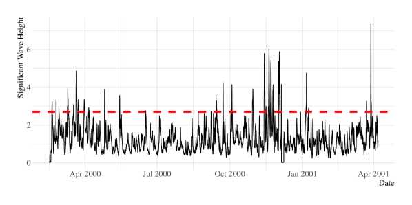
Figure 1: Significant wave height time series with hourly granularity. The red horizontal dashed line represents the exceeding threshold.

Exceedance forecasting is typically formalized as a binary classification problem, where the target variable denotes whether or not the threshold will be exceeded. Ensemble-based regression approaches can also be applied, in which the exceedance probability is estimated according to the ratio of individual predictions that exceed the threshold.

In this paper, we propose a novel approach to exceedance probabilistic forecasting. The method is based on the numeric predictions for the value of future observations produced by a forecasting model. However, the proposed method does not rely on an ensemble-based forecasting model, though it could be one. Essentially, we leverage the cumulative distribution function of the Normal distribution to estimate the exceedance probability. The location parameter of the distribution is derived from the output of the forecasting model, while the dispersion is computed on the training data. In the experiments, we also test heavy-tailed distributions which may be more suitable to model extreme values.

We resort to a case study related to SWH forecasting to validate the proposed approach. The results suggest that coupling a forecasting model with the proposed mechanism based on the cumulative distribution function is better for exceedance probability forecasting relative to a classification method or an ensemble-based forecasting model.

In summary, the contributions of this work are the following:

• A novel approach for estimating exceedance probability, which is based on the cumulative distribution function;

• The application of the method to estimate the exceedance probability of the height of waves (SWH), which is important for managing maritime operations.

The code for the methods used in the paper is publicly available. The rest of the paper is organized as follows. In Section 2, we overview the related work. In Section 3, we define the predictive problem, followed by Section 4, where we formalize the proposed method. The case study used in this work is described in Section 5. Afterward, we described the experiments carried out to validate the proposed method in Section 6. We discuss the results and conclude the paper in Section 7.

2 Related Work

In this section, we overview previous works related to ours. We start by reviewing the literature on significant wave height forecasting (Section 2.1). After, we describe approaches for probabilistic forecasting focusing on exceedance probability estimation (Section 2.2).

2.1 Significant Wave Height Forecasting

Ocean waves represent an important source of renewable energy. Information regarding the significant wave height is a key input to estimate the production of energy from waves. This is the main motivation behind several works that forecast SWH time series.

[2] use buoy data from eastern Australia. They test several regression approaches, including a model tree and multivariate adaptive regression splines, to forecast short-term (30 minutes in advance) values of SWH. They conclude that a hybrid model, optimized using a method based on least squares, provided the best performance.

[13] attempt to forecast SWH time series several hours in advance. Unlike a short-term forecast, a horizon of a few hours is important to ensure the safety of maritime operations, e.g. passage of vessels. They use the empirical mode decomposition [21] to decompose the time series into several simpler components, which are then modeled using an auto-regressive approach. This decomposition leads to better forecasting performance relative to an auto-regressive approach without this process.

[37] compared different regression algorithms for significant wave height forecasting, including artificial neural networks, support vector regression, and extreme learning machines [20]. They concluded that all methods perform comparably, though the extreme learning machine model showed a slight advantage.

Several authors attempt to apply different neural network architectures for SWH predictions, including vanilla recurrent neural networks [36], feedforward neural networks [22], gated recurrent units [44], LSTMs [44, 1, 5], or graph neural networks [12]. A comparison of these architectures is not available. But there is a tendency for recurrent architectures, which is expected due to the sequential nature of the data. In our work, we use a deep feedforward neural network, among other regression methods. We found that, in our case study, this architecture performed better than a recurrent one.

[14] and [26] also deal with smart buoy data, but their goal is to interpolate data across different buoys located in different places. When a buoy is shut down for maintenance, the data from other near buoys can be used to interpolate the missing values of that buoy.

The works mentioned so far are similar to each other in the sense that all attempt to forecast the future values or interpolate from near buoys, of SWH time series using machine learning regression models. It is difficult to compare the performance of models across different works due to the usage of different data and performance estimation methods. However, it is clear that larger forecasting horizons lead to poorer forecasting performance, as expected.

[31] also investigate the extreme values of SWH data. However, their objective is to study the statistical properties of the observations which exceed the threshold rather than try to predict them. In this work, we are interested in the future dynamics of SWH data. However, rather than predicting each instance as accurately as possible, our goal is to estimate exceedance probability. Thus, we aim at predicting if extreme values will occur at a given time period.

2.2 Exceedance Probability Forecasting

Uncertainty in the forecasts of predictive models is unavoidable. Conveying this uncertainty is critical for better decision-making. For forecasting a numeric quantity uncertainty quantification can be accomplished with prediction intervals [24], probabilistic forecasting [17], or 2D-interval predictions [42].

For binary events, we can simply output the probability of that event occurring. An instance of a binary event is exceedance, which, as mentioned before, refers to when a time series exceeds a predefined threshold.

[38] apply logistic regression to model the exceedance probability of rainfall. In their model, the lagged observations of the time series are used as predictor variables in an auto-regressive fashion.

[41] use an exceedance probability approach for financial risk management. They predict whether the returns of financial assets will exceed a threshold. This is accomplished by using a method called CARL (conditional auto-regressive logit), which is based on logistic regression. Later, CARL was extended to handle problems involving multiple thresholds by [40]. The extended model was used to predict wind ramp events, where the tails in both sides of the distribution are important to predict.

The alternative to using a classification approach to estimate the exceedance probability is to use an ensemble of forecasts. Accordingly, the probability is computed as the ratio of forecasts above the threshold. This type of approach is commonly used in fields such as meteorology [29], where different forecasts are obtained by considering different initial conditions [15]. [43] provide a comprehensive description of ensemble-based approaches listing their main properties.

Estimating the exceedance probability for different thresholds enables the construction of exceedance probability curves [25], which may be helpful for better decision-making.

Exceedance probability forecasting is related to extreme value prediction. The goal of forecasting extreme values is to accurately predict the numeric value of extreme observations in time series. For example, [34] attempt to forecast energy load spikes using a deep learning approach. On the other hand, in exceedance probability, the goal is simplified to predict whether or not a given threshold is exceeded, i.e., the magnitude of exceedance is not a major concern.

Our goal in this paper is to estimate the exceedance probability with SWH time series data. Since large waves are important to anticipate, we design an approach to estimate the probability of their occurrence. To our knowledge, this is the first attempt at framing SWH forecasting as an exceedance probability problem.

3 Problem Definition

In this section, we define the predictive task we address in this work. We start by formalizing the significant wave height forecasting task (Section 3.1), followed by the definition of exceedance probability (Section 3.2).

3.1 Time Series Forecasting

A univariate time series represents a temporal sequence of values $Y=\{y_{1},y_{2},\dots,$ $y_{n}\}$, where $y_{i}\in\mathcal{Y}\subset\mathbb{R}$ is the value of $Y$ at time $i$ and $n$ is the length of $Y$. The general goal behind forecasting is to predict the value of the upcoming observations of the time series, $y_{n+1},\ldots,y_{n+h}$, given the past observations, where $h$ denotes the forecasting horizon.

We formalize the problem of time series forecasting based on an auto-regressive strategy. Accordingly, observations of a time series are modeled based on their past recent lags. We construct a set of observations of the form ($X$, $y$) using time delay embedding according to the Takens theorem [39]. In each observation, the value of $y_{i}$ is modelled based on the most recent $q$ known values: $X_{i}=\{y_{i-1},y_{i-2},\dots,y_{i-q}\}$, where $y_{i}\in\mathcal{Y}\subset\mathbb{R}$, which represents the observation we want to predict, $X_{i}\in\mathcal{X}\subset\mathbb{R}^{q}$ represents the $i$-th embedding vector. For each horizon, the goal is to build a regression model $f$ that can be written as $y_{i}=f(X_{i},Z_{i})$, where $Z_{i}$ represents additional covariates known at the $i$-th instance. These covariates can be, for example, explanatory time series related to the phenomenon. In such a case, each of the explanatory time series is also represented at each time step $i$ with an embedding vector based on the past recent values.

3.2 Exceedance Probability Forecasting

The probability of exceedance $p_{i}$ denotes the probability that the value of a time series will exceed a predefined threshold $\tau$ in a given instant $i$. Typically, $p_{i}$ is modelled by resorting to a binary target variable $b_{i}$, which can be formalized as follows:

$$b_{i}=\begin{cases}1&\text{if }y_{i}\geq\tau,\\ 0&\text{otherwise}.\end{cases}$$ (1)

Essentially $b_{i}$ takes the value of 1 if the threshold $\tau$ is exceeded is a future period $i$, or 0 otherwise. This naturally leads to a classification problem where the goal is to build a model $g$ of the form $b_{i}=g(X_{i},Z_{i})$. Accordingly, $p_{i}$ represents the conditional expectation of $b_{i}$ which we estimate based on Bernoulli density. Logistic regression is commonly used to this effect [41].

Since the exceedance events are rare, the number of cases for the positive class (i.e. when $b_{i}=1$) is significantly smaller than the number of cases for the negative class ($b_{i}=0$). This leads to an imbalanced classification problem, which hinders the learning process of algorithms [6].

The alternative to using a classification model is to use a forecasting ensemble $F$ composed by a set of $M$ models: $F=\{f_{1},f_{2},\dots,f_{M}\}$. These models can be combined for forecasting using the uniformly weighted average as follows:

$$\hat{y}_{i}=\frac{1}{M}\sum_{k=1}^{M}f_{k}(X_{i},Z_{i})$$

We can also use the ensemble $F$ to estimate the exceedance probability according to the ratio of ensemble members that forecast a value that exceeds the threshold $\tau$:

$$p_{i}=\frac{1}{M}\sum_{k=1}^{M}I(f_{k}(X_{i},Z_{i})\geq\tau)$$

where $I$ denotes the indicator function. Hereafter, we will refer to this approach as an ensemble-based direct method for exceedance probability. Ensemble-based approaches are commonly used in some fields related to environmental science, for example, meteorology or hydrology [43].

4 Methodology

In this section, we describe the proposed approach for estimating the exceedance probability (Section 4.1). We also list the main advantages of the method relative to state-of-the-art approaches (Section 4.2).

4.1 Exceedance Probability via Cumulative Distribution Function

The goal of this work is to predict $p$, the probability that the SWH will exceed a specified threshold $\tau$. As mentioned in the introduction, large waves pose safety concerns regarding maritime operations, and it is important to anticipate them.

According to the overview of the literature we put forth in Section 2, there are two main approaches for estimating the exceedance probability: (i) using a binary classification method, or (ii) using a forecasting (regression) ensemble. In this work, we introduce a novel strategy for exceedance probability forecasting based on a time series forecasting model.

The proposed method leverages the numeric predictions produced by a forecasting model regarding the value of a future observation. Note that, while we use a forecasting (i.e. regression) approach, our method does not require an ensemble, although it could be one. Essentially, the method we describe is agnostic to the forecasting model making the predictions.

Let $\hat{y}_{i}$ denote the forecast for a future $i$-th instance. We assume that $\hat{y}_{i}$ can be modelled according to a Normal distribution with mean $\hat{y}_{i}$ and standard deviation $\sigma_{y}$: $\mathcal{N}(\hat{y}_{i},\,\sigma_{y}^{2})$. Here, $\sigma_{y}$ is computed according to the standard deviation of the training data.

In these conditions, we can estimate $p_{i}$, the exceedance probability at the $i$-th time step, using the cumulative distribution function (CDF) of $\mathcal{N}(\hat{y}_{i},\,\sigma_{y}^{2})$:

$$p_{i}=1-CDF_{\mathcal{N}(\hat{y}_{i},\,\sigma_{y}^{2})}(\tau)$$ (2)

When evaluated at the threshold $\tau$, the CDF represents the probability that the respective random variable will take a value less than or equal to $\tau$. In effect, we take the complementary value to obtain the probability that the random variable will exceed $\tau$.

We formalized this method using a Normal distribution because it works well in the case study we will present afterward. Notwithstanding, the most appropriate distribution depends on the input data.

4.2 Methodological Advantages

Aside from performance considerations, which we will delve into in Section 6, the proposed method may be preferable relative to a classifier for two main reasons. The first reason is integration because the same forecasting model can be used to predict both the upcoming values of SWH (for estimating energy production) and to estimate exceedance probability (for risk management). The second reason is threshold flexibility: a classification approach fixes the threshold during training, and it cannot be changed during inference. On the other hand, a regression model follows a lazy approach regarding the threshold. Therefore, in a given instant we can use the same model to estimate the exceedance probability for a different threshold – this enables the plotting of an exceedance probability curve.

These advantages are applicable to an ensemble-based forecasting approach. However, the high computational costs and lack of transparency often preclude the application of these strategies [27, 10].

5 Case Study

In this section, we present the case study we use in the experiments. First, we describe the data sets and their source (Section 5.1). Then, we explain the preprocessing steps carried out before applying the predictive models to the time series (Section 5.2).

5.1 Data Set

We conducted our study using data collected from the Environment and Climate Change Canada Buoy (ECCC Buoy). This buoy is located 13 kilometers away in the open sea close to Halifax, Canada. The data from this buoy was previously used for an interpolation task by [14], as we described in Section 2.1.

The time series is regularly sampled at an hourly frequency and spans from 11-02-2000 15:00:00 to 01-04-2020 11:00:00. The time series is multivariate and includes the following variables:

• SWH: Significant wave height (in meters) which represents the variable we want to predict;

• PWP: Peak wave period (in seconds), which is the wave period carrying the maximum amount of energy;

• CWH: Maximum zero crossing wave height (in meters);

• WDIR: Wind direction (in degrees);

• WSPD: Horizontal wind speed (in meters per second);

• GSPD: Gust wind speed (in meters per second);

• DRYT: Buoy dry bulb temperature (in degrees Celsius);

• SSTP: Approximated sea surface temperature (in degree Celsius).

Figure 2 shows the SWH time series. For visualization purposes, we only plot the response variable (SWH). The total number of observations is 125.890. However, there is a considerable number of missing observations, especially in the period spanning February 2016 to October 2019.

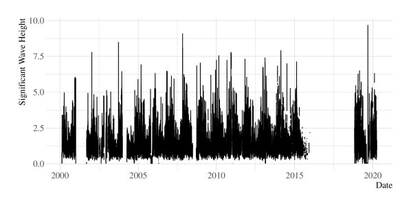
Figure 2: SWH time series captured from the ECCC buoy.

In Figure 3, we show a histogram that illustrates the distribution of the SWH time series. The distribution is right-skewed where the heavy tail represents the large waves we attempt to predict.

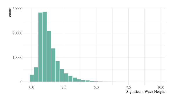
Figure 3: Histogram of the SWH time series distribution, which shows a positive skewness

5.2 Data Preparation

As exploratory data analysis, in Figure 4 we show the Pearson correlation of each pair of variables in the data set. Overall, the main variable SWH is highly correlated with CHW (0.91), and moderately correlated with the wind and gust speed variables (WSPD and GSPD) with values 0.41 and 0.42, respectively.

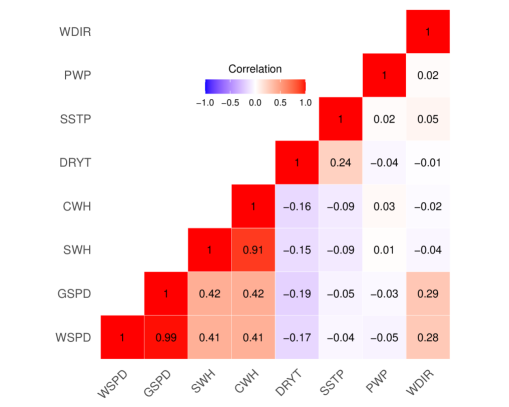
Figure 4: Heatmap showing the pairwise correlation across all variables in the data set.

We constructed a set of observations for training the predictive models according to the formalization in Section 3.1. The target variable $y$ represents the value of SWH observed $h$ steps (hours) ahead in the future. The respective binary target variable $b$ is computed according to whether $y$ takes a value above $\tau$ in $h$ hours. In order to measure the predictability of exceeding events in different time frames, we analysed multiple forecasting horizons. Specifically, we experiment with a horizon from 1 to 24 hours in advance. For example, with $h=6$ we attempt to predict whether the threshold will be exceeded in 6 hours.

In terms of the threshold $\tau$, we adopt a data-driven approach to set this value. Specifically, we set the threshold to be the 95th percentile of the available SWH time series. We follow this approach, as opposed to a judgemental one (e.g. based on some domain expert advice), because it can be generalized to different data sets or domains. In effect, at each iteration of the cross-validation procedure (which is detailed in the next section), we compute $\tau$ using the training data. The average threshold across all iterations was $3.17$ meters.

Regarding the predictor variables, we apply time delay embedding to all variables in the time series with an embedding size (number of lags) of five. This means that, at a given instant, $y$ (or $b$) is modeled according to the past five values of each of the eight variables described above. This leads to a total of 40 explanatory variables.

We also performed a data validation step. The objective is to predict exceedance events. Therefore, if exceedance is occurring in the explanatory variables ($X$) it means that the event is already happening and prediction is not necessary at that moment. In this context, we remove the instances where exceedance is occurring in the explanatory variables because the model will not be used in this case.

6 Experiments

This section describes the experiments which were designed to address the following research questions:

1. RQ1: Which approach is better for forecasting the future numeric values of the significant wave height time series?;

2. RQ2: How does the proposed CDF-based method perform for estimating the exceedance probability relative to state-of-the-art approaches?;

3. RQ3: What is the impact of the forecasting horizon on the results obtained?;

4. RQ4: Is the proposed method sensitive to different distributions?

6.1 Experimental Design

We carry out a Monte Carlo cross-validation procedure to evaluate the performance of models [33]. This estimation method, which is also referred to as repeated holdout, has been shown to provide competitive forecasting performance estimates with univariate time series [8]. Monte Carlo cross-validation is applied with 10 folds. The training and test sizes in each fold are 50% and 20% of the size of the available data, respectively. In each fold, a point is randomly selected from the available data (constrained by the size of training and testing data). This point then represents the end of the training set, and the start of the testing set [8].

We evaluate the exceedance probability performance of each approach using the area under the ROC curve (AUC) as the evaluation metric. Besides, we also use typical regression metrics to measure forecasting performance, i.e., the performance for predicting the numeric value of future observations. Specifically, we use the mean absolute error (MAE), mean absolute percentage error (MAPE), coefficient of determination ($R^{2}$), and root mean squared error (RMSE).

6.2 Methods

In this subsection, we overview the approaches used to estimate the exceedance probability. These can be broadly split into classification methods (Section 6.2.1) and forecasting (regression) methods (Section 6.2.2).

6.2.1 Classification Methods

We apply the following three classification methods for estimating exceedance probability:

• Random Forest Classifier (RFC): A standard binary classifier built using a Random Forest [7];

• Logistic Regression (LR): Another standard classifier but created using the Logistic Regression algorithm. We specifically test this method because it is a popular one for exceedance probability tasks (c.f. Section 2.2);

• RFC+SMOTE: Exceedance typically involves imbalanced problems because the exceeding events are rare. We created a variant of RFC, which attempts to cope with this issue using a resampling method. Resampling methods are popular approaches for dealing with the class imbalance problem. In effect, we test a classifier that is fit after the training data is pre-processed with the SMOTE resampling method by [11];

6.2.2 Forecasting Methods

We test four different regression approaches. Namely, a Random Forest regression method (RFR), a LASSO linear model, and a deep feed-forward neural network (NN). These are three widely used regression algorithms for forecasting. The fourth approach is a heterogeneous regression ensemble (HRE). An ensemble is referred to as heterogeneous, as opposed to homogeneous, if it is comprised of base models trained with different learning algorithms. The following learning algorithms were used to train the base models of HRE: a rule-based model based on the Cubist algorithm, a bagging ensemble of decision trees (Bagging), ridge regression (Ridge), elastic-net (ElasticNet), LASSO, multivariate adaptive regression splines (MARS), light gradient boosting optimized using random search (LGBM); extra trees (ExtraTree), Adaboost (AdaBoost), Random Forests (RFR), partial least squares regression (PLS), principal components regression (PCR), nearest neighbors (KNN), and a deep feedforward neural network (NN).

We applied different parameter settings and the total number of initial models is 50. The complete list of parameters is shown in Table 1. Using a validation set we trimmed the ensemble by removing half of the models with worse performance. The trimming process has been shown to improve the forecasting performance of ensembles [23, 9]. Usually, a dynamic combination rule improves the performance of forecasting ensembles relative to a static one. Notwithstanding, the simple average is a solid benchmark according to [9].

The neural network architecture contained 2 hidden layers with 32 and 16 units, respectively. Dropout was also included after each hidden layer with a drop rate of 0.2. All units followed a rectified linear unit activation function. Training occurred during 30 epochs. We optimized mean squared error using validation data and the Adam optimizer. The neural network experiments were carried out using the keras Python library [19]. The other algorithms listed above were training using scikit-learn [32].

Table 1: Summary of the learning algorithms

ID	Algorithm	Parameter	Value
MARS	Multivar. A. R. Splines	Degree	{1, 3}
		No. terms	{10, 20}
		Threshold	{0.01, 0.001}
LASSO	LASSO Regression	L1 alpha	{0.25, 0.5,
			0.75, 1}
Ridge	Ridge Regression	L2 alpha	{0.25, 0.5,
			0.75, 1}
ElasticNet	ElasticNet Regression	Default	-
KNN	k-Nearest Neighbors	No. of Neighbors	{1, 5, 10}
		Weights	{Uniform,
			Distance}
RFR	Random Forest Regression	No. trees	{50, 100}
		Max depth	{default, 3}
ExtraTree	Extra Trees Regression	No. trees	{50, 100}
		Max depth	{default, 3}
Bagging	Bagging Regression	Base estimator	{Decision Stump,
			Decision Tree}
		No. estimators	{50, 100}
RBR	Rule-based Regression	No. iterations	{1, 5}
NN	Deep Feedforward Neural Network	No. hidden layers	{2}
LGBM	LightGBM	Booster	{DART,
			GOSS, GBDT}
AdaBoost	AdaBoost Regression	Base estimator	{Decision Stump,
			Decision Tree}
		Learning rate	{0.3, 0.7}
PCR	Principal Comp. Regr.	No. of components	{2, 5}
PLS	Partial Least Regr.	No. of components	{2, 5}
OMP	Orthogonal Matching Pursuit	Default	-

We apply the regression approaches in two different ways in order to obtain the estimates for exceedance probability. The first is a Direct (abbreviated as D) approach: the exceedance probability $p$ is computed according to the ratio of ensemble members which predicts a value above the threshold $\tau$. The Direct approach is only valid for ensembles, in this case, HRE (a heterogeneous ensemble) and RFR (a homogeneous ensemble). The second approach is using the cumulative distribution function (CDF) according to our proposed method described in Section 4. We denote which approach is used by appending the name to the regression model. For example, HRE+CDF represents the heterogeneous ensemble applied with the cumulative distribution function for estimating exceedance probability.

6.3 Results

In this subsection, we analyse the results of the experiments. First, we analyse the performance of each regression method (RFR, LASSO, HRE, and NN) for forecasting the future values of the time series (RQ1). The results are shown in Figure 5, which illustrates the distribution of performance of each method across the forecasting horizon with four metrics: MAE, MAPE, $R^{2}$, and RMSE. For all metrics, NN and HRE show the best performance, which is comparable with each other. These methods are followed by RFR. The linear model LASSO underperforms relative to the others.

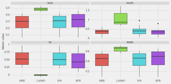
Figure 5: Distribution of forecasting performance across the forecasting horizon for each regression approach by different metrics.

We then evaluated all methods according to their ability to estimate exceedance probability. Figure 6 shows the distribution of AUC for each method across the forecasting horizons (up to 24 hours). The best performing models are NN+CDF, RFR+CDF and HRE+CDF, respectively. This rank is consistent with how these models performed for forecasting based on the regression-based scores. The results indicate that coupling a forecasting model with the mechanism based on the CDF for estimating exceedance probability provides a better performance relative to binary classification strategies (RFC, RFC+SMOTE, and LR) and ensemble-based approaches (RFR+D and HRE+D).

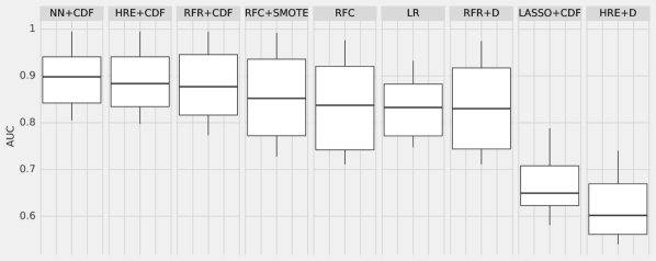
Figure 6: Distribution of the AUC for each method across the forecasting horizons.

Another interesting result to note is that HRE+D provides poor estimates regarding exceedance probability, while RFR+D is competitive with classification methods. This outcome suggests that building an ensemble with weak models (RFR is an ensemble of decision trees) is better than an ensemble of strong models, such as HRE.

Pre-processing the training data with a resampling method (SMOTE) improved the average AUC of the RFC, though the difference is small. The linear model LR is comparable with the Random Forests classifiers. On the other hand, LASSO+CDF underperforms relative to the other methods, except for HRE+D. Overall, these results answer the research question RQ2, regarding the competitiveness of the performance of a CDF-based method for estimating exceedance probability.

Figure 7: AUC for each method across the forecasting horizon. Classification methods (RFC+SMOTE, RFC, and LR) are represented with long dashed, ensemble direct methods (RFR+D, and HRE+D) are represented as dashed lines, and CDF-based methods are denoted with solid lines.

Figure 7 shows the AUC score for each method across the forecasting horizons. There is a generalized tendency for decreasing scores as the forecasting horizon increases (RQ3). This is expected as predicting further into the future represents a more difficult task.

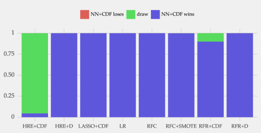
Figure 8: Results from the Bayesian correlated t-test. Probability of NN+CDF losing, drawing, or winning significantly against the respective method when considering a ROPE of 1%.

We carried out a Bayesian analysis to assess the significance of the results using the Bayesian correlated t-test [4]. This test is used to compare pairs of predictive models across the forecasting horizon. In this case, we compare NN+CDF with all remaining methods. We define the region of practical equivalence (ROPE) for the Bayes correlated t-test to be the interval [-1%, 1%]. This means that the performance of the two methods under comparison is considered equivalent if their percentage difference is within this interval. The results are presented in Figure 8, which shows the probability of NN+CDF winning in blue, drawing in green (results within the ROPE), or losing in red against each remaining method. NN+CDF outperforms other approaches, except for HRE+CDF. Notwithstanding, the ensemble HRE+CDF also follows the proposed approach for exceedance probability forecasting.

Figure 9: Average scores for each distribution and classification metric across the forecasting horizon.

In the previous experiments, we used the CDF of the Normal distribution $\mathcal{N}(\hat{y}_{i},\,\sigma_{y}^{2})$ at each $i$-th instance.

We studied the sensitivity of the proposed method to different distributions. We focused on continuous distributions with location and scale parameters, which we set to $\hat{y}_{i}$ and $\sigma_{y}$, respectively. Besides the Normal, we tested the following distributions: Gumbel, Cauchy, Laplace, Logistic, Lognormal, and Rayleigh. These have heavier tails relative to the Normal, which may be important because the tails are usually relevant in exceedance probability forecasting tasks. We present the results in Figure 9. Besides the average AUC across the horizon, we also include the average of standard classification metrics, namely precision, recall, and F1-score. These were obtained by using 0.5 as a decision threshold, which is the typical default value. Varying the distribution does not have an impact in terms of AUC scores. This means that, from a probabilistic perspective, all distribution lead to similar results. All distributions behave similarly for ranking the observations according to their probability of representing an exceedance event. However, the class predictions lead to different results in terms of classification. This outcome can be justified by different calibration profiles of the distinct distributions, which are caused by the different CDF curves. Overall, the Gumbel and Normal distributions lead to the best F1-scores (RQ4).

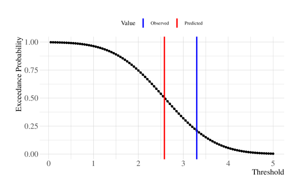
Figure 10: Exceedance probability curve for a given example instance where exceedance occurs. The red vertical bar is the predicted value and the blue vertical bar is the observed value.

Finally, we draw the exceedance probability curve in Figure 10 for a given test instance to exemplify the dynamics of the probabilities across different thresholds. The predicted and observed value for that instance are represented as the red and blue vertical bars, respectively. In this example, we compute the exceedance probability using the proposed CDF-based approach. The point forecast is about 2.55. According to our normality assumption, the exceedance probability at that point is 50%. We then compute this probability for different points, which leads to a curve with the form of the Normal CDF. Given the predicted value, it is almost certain that threshold 1 will be exceeded. The threshold 2 will be exceeded with a 75% probability. The actual value (around 3.3) had a probability of about 24% of occurring according to the model.

7 Final Remarks

We proposed a new method to estimate exceedance probability using the numeric predictions obtained from a forecasting model. This approach is an alternative to using a binary classification model or an ensemble-based approach.

The main conclusion is that the proposed method provides better exceedance probability estimates relative to the alternatives listed above for a case study in the ocean data domain (SWH forecasting). This outcome has an important practical impact because users (e.g. decision-makers or analysts responsible for maritime operations) can rely on a forecasting model to predict not only the value of future observations but also quantify the probability of an exceedance event (in this case, a large wave).

A second important conclusion is that a deep learning neural network provided the best results when coupled with the proposed approach. Besides, a heterogeneous regression ensemble (HRE), whose members are trained with several different learning algorithms, did not provide better exceedance probability estimations than a Random Forest (RFR).

While exceedance probability forecasting usually refers to binary events (whether or not the exceedance occurs), multiple thresholds can also be defined. An example of this is the triple barrier method used in quantitative trading, e.g. [3, 35]. Stock market traders may be interested in predicting buy, sell, or hold signals according to price movements. Exceeding a positive threshold in terms of predicted price returns can be used as a buy signal; the opposite (predicted price returns below a negative threshold) can represent a sell trigger. If none of the thresholds is met, then the trader should hold the current position.

Using Monte Carlo simulation is a common procedure to estimate the probability of events. In this work, we follow an analytical approach based on the CDF. As we assume a particular distribution to predict or estimate its parameters, our solution is computationally cheap. Using the same distribution with equivalent parameters, a Monte Carlo approximation leads to equivalent results.

We transformed the time series into a trainable format using time delay embedding on each variable, as we formalized in Section 3. During our experiments, we also tested two preprocessing steps: a differencing operation to remove the trend and stabilize the mean, and a Box-Cox power transformation to stabilize the variance. Since neither of these processes improved performance we excluded them in the final experiments.

Finally, the proposed approach settled on the cumulative Normal distribution function. However, the data showed a clear positive skewness. This leads us to try different distributions designed for extreme values. We did not find significant differences between different distributions. Notwithstanding, we believe that the most appropriate distribution strongly depends on the input data.

References

- Abdullah et al. [2022] Abdullah, F., Ningsih, N., & Al-Khan, T. (2022). Significant wave height forecasting using long short-term memory neural network in indonesian waters. Journal of Ocean Engineering and Marine Energy, 8, 183–192.
- Ali et al. [2020] Ali, M., Prasad, R., Xiang, Y., & Deo, R. C. (2020). Near real-time significant wave height forecasting with hybridized multiple linear regression algorithms. Renewable and Sustainable Energy Reviews, 132, 110003.
- Baía & Torgo [2017] Baía, L., & Torgo, L. (2017). A comparative study of approaches to forecast the correct trading actions. Expert Systems, 34, e12169.
- Benavoli et al. [2017] Benavoli, A., Corani, G., Demšar, J., & Zaffalon, M. (2017). Time for a change: a tutorial for comparing multiple classifiers through bayesian analysis. The Journal of Machine Learning Research, 18, 2653–2688.
- [5] Bethel, B. J., Dong, C., Zhou, S., Sun, W., & Bao, Y. (). Assessing long short-term memory network significant wave height forecast efficacy in the caribbean sea and atlantic ocean. Available at SSRN 4153300, .
- Branco et al. [2016] Branco, P., Torgo, L., & Ribeiro, R. P. (2016). A survey of predictive modeling on imbalanced domains. ACM Computing Surveys (CSUR), 49, 1–50.
- Breiman [2001] Breiman, L. (2001). Random forests. Machine learning, 45, 5–32.
- Cerqueira et al. [2020] Cerqueira, V., Torgo, L., & Mozetič, I. (2020). Evaluating time series forecasting models: An empirical study on performance estimation methods. Machine Learning, 109, 1997–2028.
- Cerqueira et al. [2019] Cerqueira, V., Torgo, L., Pinto, F., & Soares, C. (2019). Arbitrage of forecasting experts. Machine Learning, 108, 913–944.
- Cerqueira et al. [2021] Cerqueira, V., Torgo, L., Soares, C., & Bifet, A. (2021). Model compression for dynamic forecast combination. arXiv preprint arXiv:2104.01830, .
- Chawla et al. [2002] Chawla, N. V., Bowyer, K. W., Hall, L. O., & Kegelmeyer, W. P. (2002). Smote: synthetic minority over-sampling technique. Journal of artificial intelligence research, 16, 321–357.
- Chen et al. [2021] Chen, D., Liu, F., Zhang, Z., Lu, X., & Li, Z. (2021). Significant wave height prediction based on wavelet graph neural network. In 2021 IEEE 4th International Conference on Big Data and Artificial Intelligence (BDAI) (pp. 80–85). IEEE.
- Duan et al. [2016] Duan, W.-y., Huang, L.-m., Han, Y., & Huang, D.-t. (2016). A hybrid emd-ar model for nonlinear and non-stationary wave forecasting. Journal of Zhejiang University-SCIENCE A, 17, 115–129.
- Fasuyi et al. [2020] Fasuyi, J. W., Newport, J., & Whidden, C. (2020). A machine learning redundancy model for the herring cove smart buoy. Journal of Ocean Technology, 15.
- Ferro [2007] Ferro, C. A. (2007). Comparing probabilistic forecasting systems with the brier score. Weather and Forecasting, 22, 1076–1088.
- Frangopol & Kim [2014] Frangopol, D., & Kim, S. (2014). Prognosis and life-cycle assessment based on shm information. In Sensor technologies for civil infrastructures (pp. 145–171). Elsevier.
- Gneiting & Katzfuss [2014] Gneiting, T., & Katzfuss, M. (2014). Probabilistic forecasting. Annual Review of Statistics and Its Application, 1, 125–151.
- Granger & Pesaran [2000] Granger, C. W., & Pesaran, M. H. (2000). Economic and statistical measures of forecast accuracy. Journal of Forecasting, 19, 537–560.
- Gulli & Pal [2017] Gulli, A., & Pal, S. (2017). Deep learning with Keras. Packt Publishing Ltd.
- Huang et al. [2006] Huang, G.-B., Zhu, Q.-Y., & Siew, C.-K. (2006). Extreme learning machine: theory and applications. Neurocomputing, 70, 489–501.
- Huang et al. [1998] Huang, N. E., Shen, Z., Long, S. R., Wu, M. C., Shih, H. H., Zheng, Q., Yen, N.-C., Tung, C. C., & Liu, H. H. (1998). The empirical mode decomposition and the hilbert spectrum for nonlinear and non-stationary time series analysis. Proceedings of the Royal Society of London. Series A: mathematical, physical and engineering sciences, 454, 903–995.
- Jain & Deo [2007] Jain, P., & Deo, M. (2007). Real-time wave forecasts off the western indian coast. Applied ocean research, 29, 72–79.
- Jose & Winkler [2008] Jose, V. R. R., & Winkler, R. L. (2008). Simple robust averages of forecasts: Some empirical results. International journal of forecasting, 24, 163–169.
- Khosravi et al. [2011] Khosravi, A., Nahavandi, S., Creighton, D., & Atiya, A. F. (2011). Comprehensive review of neural network-based prediction intervals and new advances. IEEE Transactions on neural networks, 22, 1341–1356.
- Kunreuther [2002] Kunreuther, H. (2002). Risk analysis and risk management in an uncertain world 1. Risk Analysis: An International Journal, 22, 655–664.
- Kuppili [2021] Kuppili, A. S. (2021). Forecasting meteorological variables and anticipating climatic aberrations of an oceanic buoy using a neighbour buoy, .
- Lakkaraju et al. [2016] Lakkaraju, H., Bach, S. H., & Leskovec, J. (2016). Interpretable decision sets: A joint framework for description and prediction. In Proceedings of the 22nd ACM SIGKDD international conference on knowledge discovery and data mining (pp. 1675–1684).
- Lambert et al. [1994] Lambert, J. H., Matalas, N. C., Ling, C. W., Haimes, Y. Y., & Li, D. (1994). Selection of probability distributions in characterizing risk of extreme events. Risk Analysis, 14, 731–742.
- Lewis [2005] Lewis, J. M. (2005). Roots of ensemble forecasting. Monthly weather review, 133, 1865–1885.
- Li et al. [2012] Li, G., Weiss, G., Mueller, M., Townley, S., & Belmont, M. R. (2012). Wave energy converter control by wave prediction and dynamic programming. Renewable Energy, 48, 392–403.
- Méndez et al. [2006] Méndez, F. J., Menéndez, M., Luceño, A., & Losada, I. J. (2006). Estimation of the long-term variability of extreme significant wave height using a time-dependent peak over threshold (pot) model. Journal of Geophysical Research: Oceans, 111.
- Pedregosa et al. [2011] Pedregosa, F., Varoquaux, G., Gramfort, A., Michel, V., Thirion, B., Grisel, O., Blondel, M., Prettenhofer, P., Weiss, R., Dubourg, V. et al. (2011). Scikit-learn: Machine learning in python. the Journal of machine Learning research, 12, 2825–2830.
- Picard & Cook [1984] Picard, R. R., & Cook, R. D. (1984). Cross-validation of regression models. Journal of the American Statistical Association, 79, 575–583.
- Polson & Sokolov [2020] Polson, M., & Sokolov, V. (2020). Deep learning for energy markets. Applied Stochastic Models in Business and Industry, 36, 195–209.
- de Prado [2020] de Prado, M. M. L. (2020). Machine learning for asset managers. Cambridge University Press.
- Sadeghifar et al. [2017] Sadeghifar, T., Nouri Motlagh, M., Torabi Azad, M., & Mohammad Mahdizadeh, M. (2017). Coastal wave height prediction using recurrent neural networks (rnns) in the south caspian sea. Marine Geodesy, 40, 454–465.
- Shamshirband et al. [2020] Shamshirband, S., Mosavi, A., Rabczuk, T., Nabipour, N., & Chau, K.-w. (2020). Prediction of significant wave height; comparison between nested grid numerical model, and machine learning models of artificial neural networks, extreme learning and support vector machines. Engineering Applications of Computational Fluid Mechanics, 14, 805–817.
- Slud & Kedem [1994] Slud, E., & Kedem, B. (1994). Partial likelihood analysis of logistic regression and autoregression. Statistica Sinica, (pp. 89–106).
- Takens [1981] Takens, F. (1981). Dynamical systems and turbulence, warwick 1980: Proceedings of a symposium held at the university of warwick 1979/80. chapter Detecting strange attractors in turbulence. (pp. 366–381). Berlin, Heidelberg: Springer Berlin Heidelberg.
- Taylor [2017] Taylor, J. W. (2017). Probabilistic forecasting of wind power ramp events using autoregressive logit models. European Journal of Operational Research, 259, 703–712.
- Taylor & Yu [2016] Taylor, J. W., & Yu, K. (2016). Using auto-regressive logit models to forecast the exceedance probability for financial risk management. Journal of the Royal Statistical Society: Series A (Statistics in Society), 179, 1069–1092.
- Torgo & Ohashi [2011] Torgo, L., & Ohashi, O. (2011). 2d-interval predictions for time series. In Proceedings of the 17th ACM SIGKDD international conference on Knowledge discovery and data mining (pp. 787–794).
- Toth et al. [2003] Toth, Z., Talagrand, O., Candille, G., & Zhu, Y. (2003). Probability and ensemble forecasts. Forecast verification: A practitioner’s guide in atmospheric science, 137, 163.
- Wang et al. [2021] Wang, J., Wang, Y., & Yang, J. (2021). Forecasting of significant wave height based on gated recurrent unit network in the taiwan strait and its adjacent waters. Water, 13, 86.