latexReferences

Double soft-thresholded model for multi-group scalar on vector-valued image regression

Abstract: In this paper, we develop a novel spatial variable selection method for scalar on vector-valued image regression in a multi-group setting. Here, ‘vector-valued image’ refers to the imaging datasets that contain vector-valued information at each pixel/voxel location, such as in RGB color images, multimodal medical images, DTI imaging, etc. The focus of this work is to identify the spatial locations in the image having an important effect on the scalar outcome measure. Specifically, the overall effect of each voxel is of interest. We thus develop a novel shrinkage prior by soft-thresholding the $\ell_{2}$ norm of a latent multivariate Gaussian process. It allows us to estimate sparse and piecewise-smooth spatially varying vector-valued regression coefficient function. Motivated by the real data, we further develop a double soft-thresholding based framework when there are multiple pre-specified subgroups. For posterior inference, an efficient MCMC algorithm is developed. We compute the posterior contraction rate for parameter estimation and also establish consistency for variable selection of the proposed Bayesian model, assuming that the true regression coefficients are Hölder smooth. Finally, we demonstrate the advantages of the proposed method in simulation studies and further illustrate in an ADNI dataset for modeling MMSE scores based on DTI-based vector-valued imaging markers.

Keywords: Image regression, Multi-group, Neuroimaging, Posterior consistency, scalar on image regression, Soft-thresholding, Variable selection.

1 Introduction

Many modern imaging applications collect vector-valued image data, where each spatial location contains more than one scalar information. The vector-valued images are more appealing in recent biomedical applications. For example, in biomedical imaging, vector-valued imaging markers are routinely collected by multimodal imaging methods. As an example, modern medical scanning devices such as SPECT/CT compute single-photon emission computed tomography (SPECT) and computed tomography (CT) together at each spatial location (Ehrhardt and Arridge, 2013). Apart from the multimodal imaging, there are now several medical imaging methods that collect RGB based color images (Bajaj et al., 2001; Lange, 2005; Qi et al., 2011; Jones et al., 2017). Hence, the contrast at each imaging location is represented by a vector instead of a scalar. For some immunohistochemistry (IHC) assay (Feldman and Wolfe, 2014), the RGB information can be further converted into the underlying staining (e.g, hematoxylin and eosin staining) revealing more biomedically informative information.

Our paper is particularly motivated by a medical imaging application called the diffusion tensor imaging (DTI) (Soares et al., 2013). In this imaging technique, various types of vector-valued imaging markers are assessed to describe white matter tissue properties in the brain. The main purpose of DTI is to identify the white matter anatomical structure of the whole brain derived from diffusion tensor signals. A quantity to describe the spatial specific anatomical structure is ${\mathbf{M}}({\mathbf{v}})$, a $3\times 3$ positive definite (pd) matrix, called the diffusion tensor at location ${\mathbf{v}}$. The eigenvectors of these matrices represent the diffusion directions, $[{\mathbf{e}}_{1}\ {\mathbf{e}}_{2}\ {\mathbf{e}}_{3}]$ and the squared roots of the eigenvalues $[l_{1}\ l_{2}\ l_{3}]$ are the corresponding semi-axis lengths (Zhou, 2010, Section 1.2.3). In many recent works, the principal eigenvector ${\mathbf{M}}({\mathbf{v}})$ is used to describe the structural information, known as diffusion direction (Wong et al., 2016). Several works have established the clinical significance of summary measurements derived from diffusion tensors. In the usual route of inference using DTI data, white matter structural connectivity profiles are first derived by reconstructing the fiber tracts using tractography algorithms on the DTI-derived estimates (Wong et al., 2016). Subsequently, a low-resolution summary of the network, called connectome (Sporns, 2011) is usually constructed using these profiles assuming some parcellation of the brain. In clinical applications, their associations with the subject’s covariates are studied. However, such summarization may contain biases, which could lead to inefficient statistical inference. Thus, in this work, we focus on analyzing the effects of the DTI-derived principal diffusion direction markers directly on the performance based mini mental state examination (MMSE) score. Due to a large number of predictors in an imaging dataset, it is prudent to employ regularized regression techniques for reasonable inference. On the other hand, the spatial dependence among the image predictors further prompts us to assume that the regression effects of the neighboring voxels should be close.

Hence, the primary challenges require to be addressed are: 1) handling imaging predictors having vector-valued information at each voxel location, 2 tackling complex spatial dependence of the data, and 3) identifying regression effects that are simultaneously sparse and continuous, where sparsity is defined in terms of the number of non-zero smooth pieces in it. We let ${\mathbf{D}}_{i}({\mathbf{v}})$ be a $q$-dimensional vector-valued predictor for $i$-$th$ subject at location ${\mathbf{v}}$, and it can be applied to any avector-valued image data. In our DTI application, ${\mathbf{D}}_{i}({\mathbf{v}})$ are principal diffusion direction i.e. first eigenvector of ${\mathbf{M}}({\mathbf{v}})$. Since the components within ${\mathbf{D}}_{i}({\mathbf{v}})$ can only be put together to illustrate the diffusion direction within a voxel, each component of the multidimensional vector-valued predictor ${\mathbf{D}}_{i}({\mathbf{v}})$ can not be of direct interest. Therefore, identifying the spatial locations ${\mathbf{v}}$ having important overall effects on the scalar outcomes is our primary goal.

To characterize a possible relation between a scalar outcome and an imaging predictor, scalar on image regression models are widely popular (Goldsmith et al., 2014; Li et al., 2015; Wang and Zhu, 2017; Kang et al., 2018). Following the traditional scalar on image regression setting, the effect of a voxel ${\mathbf{v}}$ can be quantified by ${\mathbf{D}}_{i}({\mathbf{v}})^{T}\mbox{\boldmath$\beta$}({\mathbf{v}})$, where $\mbox{\boldmath$\beta$}({\mathbf{v}})$ stands for the regression effect of the ${\mathbf{v}}$-$th$ voxel and $<{\mathbf{x}},{\mathbf{y}}>$ stand for the inner product between ${\mathbf{x}}$ and ${\mathbf{y}}$. This can be rewritten as ${\mathbf{D}}_{i}({\mathbf{v}})^{T}\mbox{\boldmath$\beta$}({\mathbf{v}})=\|{\mathbf{D}}_{i}({\mathbf{v}})\|_{2}\|\mbox{\boldmath$\beta$}({\mathbf{v}})\|_{2}\cos(\theta_{{\mathbf{D}}_{i}({\mathbf{v}}),\mbox{\boldmath$\beta$}({\mathbf{v}})}),$ where $\theta_{{\mathbf{D}}_{i}({\mathbf{v}}),\mbox{\boldmath$\beta$}({\mathbf{v}})}$ is the geometric angle between the two vectors ${\mathbf{D}}_{i}({\mathbf{v}})$ and $\mbox{\boldmath$\beta$}({\mathbf{v}})$. Here $\|\mbox{\boldmath$\beta$}({\mathbf{v}})\|_{2}\cos(\theta_{{\mathbf{D}}_{i}({\mathbf{v}}),\mbox{\boldmath$\beta$}({\mathbf{v}})})$ can be interpreted as the rate of change of ${\mathbf{D}}_{i}({\mathbf{v}})^{T}\mbox{\boldmath$\beta$}({\mathbf{v}})$ for unit change in $\|{\mathbf{D}}_{i}({\mathbf{v}})\|_{2}$. Thus, $\|\mbox{\boldmath$\beta$}({\mathbf{v}})\|_{2}$ can be considered as the universal “magnitude” that the voxel ${\mathbf{v}}$ contributes to the unit change in the scalar outcome. However, given each individual’s ${\mathbf{D}}_{i}({\mathbf{v}})$, the total contribution varies from one subject to the other depending on $\cos(\theta_{{\mathbf{D}}_{i}({\mathbf{v}}),\mbox{\boldmath$\beta$}({\mathbf{v}})})$. Apart from the vector-valued image regression application, the proposed model can be feasibly applied in several other avenues of image regression. In Section 7, we illustrate an interesting application of our proposed model for estimating sparse nonparametric additive scalar on image regression model, which will be one of our future directions.

Since the voxel-wise overall effect is of our main interest, we consider that the norm $\|\mbox{\boldmath$\beta$}({\mathbf{v}})\|_{2}$ here is the overall effect that tells us whether the voxel ${\mathbf{v}}$ is a good predictor in general or not. If it is 0, then none of the components in ${\mathbf{D}}_{i}({\mathbf{v}})$ have any predictive importance, and thus we should not consider that voxel (region) in our predictive model. Furthermore, variable selection for each of the individual coefficient functions may not be possible due to the dependence among the components in ${\mathbf{D}}_{i}({\mathbf{v}})$. However, it is evident that the set of predictors at each voxel naturally forms a group. Hence, a reasonable model for our regression problem can be formulated using group-LASSO (Yuan and Lin, 2006). However, the spatial dependence among the predictors will prevent the usage of traditional group-LASSO. Hence, we propose a novel spatial variable selection prior for $\mbox{\boldmath$\beta$}(\cdot)$ through a soft-thresholding transformation on the $\ell_{2}$ norm of a latent $q$-dimensional spatially varying function $\widetilde{\mbox{\boldmath$\beta$}}(\cdot)$ and the latent spatially varying function is assumed to follow a Gaussian process with a scaled squared exponential kernel (van der Vaart and van Zanten, 2009).

In general, sparse estimation is an important statistical problem, and there are considerable numbers of competing methods. In a frequentist setting, different types of regularization or penalty functions are used for sparse estimation (Tibshirani, 1996; Tibshirani et al., 2005). On the other hand, in a Bayesian framework, several types of sparsity-inducing priors have been introduced such as the traditional spike and slab prior (Mitchell and Beauchamp, 1988), the horseshoe prior (Carvalho et al., 2010), normal-gamma prior (Griffin and Brown, 2010), double-Pareto prior (Armagan et al., 2013) or Dirichlet-Laplace prior (Bhattacharya et al., 2015). However, these priors are not suitable for an imaging predictor and the regression effect is expected to be spatially smooth.

Goldsmith et al. (2014) and Li et al. (2015) proposed priors that account for spatial dependence and sparsity for scalar on image regression models separately. To a related problem, Wang and Zhu (2017) proposed a penalty based on the total variation. Spatial dependence, however, is still not fully incorporated in this approach. Recently, Roy et al. (2021) developed a prior that is suitable to estimate piece-wise sparse signals. In Kang et al. (2018), a soft-thresholded Gaussian process prior was proposed for a related problem. Soft-thresholding induced sparse estimation is widely popular in various application areas (Fan and Li, 2001; Han et al., 2006; Rothman et al., 2009; Kusupati et al., 2020). Thresholding based Bayesian modeling approaches are getting increasing popularity (ni2019bayesian; cai2020bayesian; wu2022bayesian). Our modeling approach also relies on a novel soft-thresholding transformation. Furthermore, we extend the model for a multi-group setting to efficiently characterize the group structure of the data. Kang et al. (2018) further proposed to use low-rank approximations for handling large neuroimaging datasets and developed a Metropolis-Hastings-based Markov chain Monte Carlo (MCMC) sampling algorithm. We, too, consider using low-rank approximations for faster computation and in addition, implement a gradient-based Hamiltonian Monte Carlo (HMC) sampling algorithm (Neal, 2011) for efficient posterior computation.

Furthermore, we establish posterior contraction rates, which provide us with new insights for soft-thresholded estimates. Our results are different from those of Kang et al. (2018). They are built on a very different set of assumptions on the predictor process and also consider the thresholding parameter to be an unknown parameter, unlike Kang et al. (2018). For image regression, the predictor process plays an important role. Our assumptions on the predictor process are motivated by the developments in the sparse covariance matrix estimation theory (Bickel and Levina, 2008a, b). Under those assumptions, we are able to establish strong consistency results with respect to the following distance $d(\mbox{\boldmath$\beta$},\mbox{\boldmath$\beta$}_{0})=\int_{{\mathbf{v}}}\|\mbox{\boldmath$\beta$}({\mathbf{v}})-\mbox{\boldmath$\beta$}_{0}({\mathbf{v}})\|_{2}{\mathrm{d}}{\mathbf{v}}$. We also establish the spatial variable selection consistency results. For adaptive estimation, we consider the scaled square exponential kernel based Gaussian process prior for our latent coefficient function $\widetilde{\mbox{\boldmath$\beta$}}(\cdot)$ and borrow a few results from van der Vaart and van Zanten (2009).

The rest of the article is organized as follows. In the next section, we present our proposed modeling framework and describe some of its properties. In Section 3, we study the large sample properties of our proposed method. Detail descriptions of the priors and the posterior computation steps are in Section 4 In Section 5, we compare the performance of our proposed method with other competing methods. We present our ADNI data application in Section 6. Finally, in Section 7, we discuss possible extensions, and other future directions.

2 Modeling framework

In many real data applications for scientific and clinical investigation (e.g., ADNI), the data are collected from several heterogeneous groups. We thus introduce our scalar on vector-valued image regression model for a multi-group dataset, described as follows. Let, $y_{i}$ be the scalar response for $i$-$th$ subject and ${\mathbf{D}}_{i}({\mathbf{v}}_{j})$ be the $q$-dimensional spatially distributed imaging predictor which is collected at the $d$-dimensional spatial location ${\mathbf{v}}_{j}$ where $j=1,\ldots,p$. Our goal is to identify important predictors ${\mathbf{D}}_{i}({\mathbf{v}}_{j})$ driving the scalar response $y_{i}$. We assume that the set of spatial locations $\{{\mathbf{v}}_{j}\}_{j=1}^{p}$ are from a compact closed region ${\cal B}\in\mathbb{R}^{d}$ to allow us to define a spatial process with indices of $\{{\mathbf{v}}_{j}\}_{j=1}^{p}$. Let us further assume that there are $G$ many groups. Let us further define the sets $\{{\cal G}_{1},\ldots,{\cal G}_{G}\}$, where ${\cal G}_{g}$ stand for the set of subject indices that belong to the $g$-$th$ group. To this end, we introduce our proposed scalar on vector-valued image regression model as,

$$y_{i}= b_{0,g}+p^{-1/2}\sum_{j=1}^{p}{\mathbf{D}}_{i}({\mathbf{v}}_{j})^{T}\mbox{\boldmath$\beta$}_{g}({\mathbf{v}}_{j})+e_{i},\textrm{ for }i\in g$$ (1)

$$e_{i}\sim \hbox{Normal}(0,\sigma^{2})$$

where $b_{0,g}$’s stand for group-specific intercepts, and $\mbox{\boldmath$\beta$}_{g}({\mathbf{v}}_{j})$’s are the group specific spatially varying vector valued regression coefficient to characterize effects of ${\mathbf{D}}_{i}({\mathbf{v}}_{j})$ on $y_{i}$ when $i$-$th$ belongs to $g$-$th$ group. Here, ${\mathbf{D}}_{i}({\mathbf{v}}_{j})^{T}\mbox{\boldmath$\beta$}_{g}({\mathbf{v}}_{j})$ stands for the effect ${\mathbf{v}}_{j}$-$th$ voxel for $g$-$th$ group. The normalizing constant $p^{-1/2}$ is to scale down the total effects of massive imaging predictors following Kang et al. (2018). We maintain group-specific separate intercepts $b_{0,g}$’s in the model. This specification allows flexible interpretation of the coefficients without setting the reference group. Returning to the decomposition, ${\mathbf{D}}_{i}({\mathbf{v}})^{T}\mbox{\boldmath$\beta$}_{g}({\mathbf{v}})=\|{\mathbf{D}}_{i}({\mathbf{v}})\|_{2}\|\mbox{\boldmath$\beta$}_{g}({\mathbf{v}})\|_{2}\cos(\theta_{{\mathbf{D}}_{i}({\mathbf{v}}),\mbox{\boldmath$\beta$}_{g}({\mathbf{v}})}),$ we can see that the part $\|\mbox{\boldmath$\beta$}_{g}({\mathbf{v}})\|_{2}\cos(\theta_{{\mathbf{D}}_{i}({\mathbf{v}}),\mbox{\boldmath$\beta$}_{g}({\mathbf{v}})})$ is the effect of ${\mathbf{v}}$-$th$ spatial location for $i$-$th$ subject, and it varies with the data vector’s direction. Specifically, the part $\cos(\theta_{{\mathbf{D}}_{i}({\mathbf{v}}),\mbox{\boldmath$\beta$}_{g}({\mathbf{v}})})$ controls the variation across the subjects, as well as the sign. For some individuals, the overall contribution may be positive and for some, it may be negative. This may also be of clinical importance to know, for which individuals the effect of ${\mathbf{v}}$-$th$ location is positive and for whom it is negative based on the estimated effect $\hat{\mbox{\boldmath$\beta$}}_{g}({\mathbf{v}})$. We discuss these directions in the following subsections. The error variance $\sigma$ is kept fixed for all the groups, which may be relaxed. However, in this paper, we do not consider that.

Different from traditional scalar on image regression where the predictor at each location is a scalar, our imaging predictor has vector-valued entries at each spatial location. In the next subsection, we first introduce our proposed soft-thresholding transformation-based characterization to model sparse vector-valued spatially varying regression coefficients. Building on that, we subsequently propose our prior model for $\mbox{\boldmath$\beta$}_{g}(\cdot)$ in the multi-group case, suitable for estimating sparse and piece-wise smooth coefficients.

2.1 Soft-Thresholded $\ell_{2}$ Norm transformation

The regression coefficients $\mbox{\boldmath$\beta$}_{g}$’s are vector-valued, and they are assumed to be piecewise smooth and sparse to accommodate the desired properties in high dimensional scalar on image regression. We propose a soft-thresholding transformation based prior model for $\mbox{\boldmath$\beta$}_{g}$. Due to the vector-valued characteristic, we first define our soft-thresholding function for a $q$-dimensional vector ${\mathbf{x}}$ as $h_{\lambda}({\mathbf{x}})=\left(1-\frac{\lambda}{\|{\mathbf{x}}\|_{2}}\right)_{+}{\mathbf{x}}$ . Since it puts the thresholding on the $\ell_{2}$ norm, we call this transformation Soft-Thresholded $\ell_{2}$ Norm (ST2N) transformation. Figure 1 depicts how ST2N thresholds the original vector in a 2D case. Finally, we model $\mbox{\boldmath$\beta$}({\mathbf{v}})$ as the ST2N transformation of a multivariate Gaussian process (GP) $\widetilde{\mbox{\boldmath$\beta$}}({\mathbf{v}})$ such that $\mbox{\boldmath$\beta$}({\mathbf{v}})=h_{\lambda}(\widetilde{\mbox{\boldmath$\beta$}}({\mathbf{v}}))$. Hence, our final prior for $\mbox{\boldmath$\beta$}({\mathbf{v}})$ is termed as ST2N-GP.

Here $Q_{\lambda}(s)=\Pi(\|\widetilde{\mbox{\boldmath$\beta$}}(v)\|<\lambda)$ is the prior probability associated with the event $\mbox{\boldmath$\beta$}({\mathbf{v}})=0$. We thus have $Q_{\lambda_{1}}(s)<Q_{\lambda_{2}}(s)$ for $\lambda_{1}<\lambda_{2}$. Thus, greater thresholding induces greater prior mass at zero. Our motivating dataset further has a multi-group structure. Hence, in the following subsection, we propose a novel double soft-thresholding transformation to accommodate multi-group data. In the following Lemma, we show continuity of the proposed soft-thresholding transformation that ensures continuity of the transformed coefficient $\mbox{\boldmath$\beta$}(\cdot)$ when the underlying latent function $\widetilde{\mbox{\boldmath$\beta$}}(\cdot)$ is smooth. Continuity is a desired property for $\mbox{\boldmath$\beta$}(\cdot)$ as discussed before.

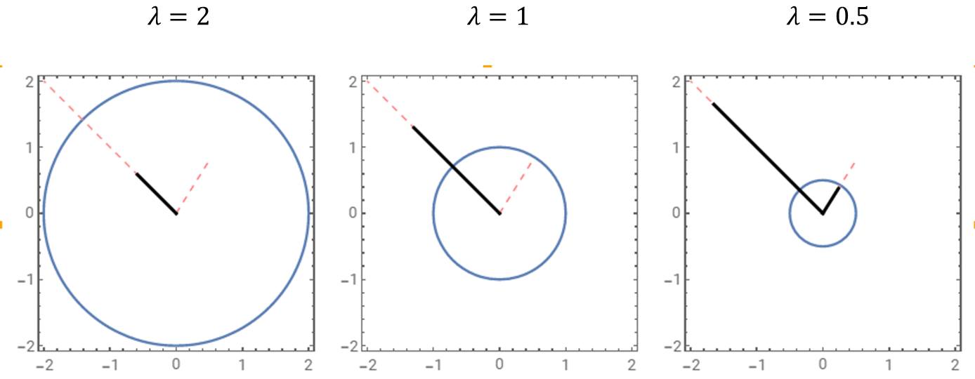
Figure 1: ST2N in action: Here the effect of the thresholding parameter $\lambda$ is illustrated for its three possible values, and the vectors are in 2-D ($q=2$). The dashed red line is the original vector ${\mathbf{x}}$ and solid black line stands for its ST2N transformation, $h_{\lambda}({\mathbf{x}})$. We can see that the vector with shorted magnitude is transformed to the origin when $\lambda=2$ and 1.

Lemma 1 (Lipchitz Continuity).

The ST2N transformation is Lipchitz continuous.

The proof is in the appendix. We show Lipchitz continuity both under $\ell_{2}$ and $\ell_{\infty}$ norms. By construction, ST2N transformation only shrinks the magnitude, but does not alter the direction. We thus have $\|h_{\lambda}({\mathbf{x}})\|_{2}=(\|{\mathbf{x}}\|_{2}-\lambda)_{+}$, but $\frac{h_{\lambda}({\mathbf{x}})}{\|h_{\lambda}({\mathbf{x}})\|_{2}}=\frac{{\mathbf{x}}}{\|{\mathbf{x}}\|_{2}}$ whenever $\|{\mathbf{x}}\|_{2}>\lambda$.

2.2 Double soft-thresholding for multi-group

Building on our proposed ST2N transformation, we now propose our prior model for $\mbox{\boldmath$\beta$}_{g}(\cdot)$. Our inferential objective here is to identify the spatial locations having an important effect on the scalar response. For different groups, the set of important spatial locations can be different. While modeling multi-group data, one of the groups is set as a reference in typical clinical studies. However, the choice of a reference group may not be easy in certain cases. For example, if the groups are representing different stages of a disease, it is then ambiguous to select which one should be the reference group. Our real data application also represents such a scenario, where we consider three different stages of cognitive impairment as different clinical groups of Alzheimer’s disease. The proposed multi-group model is thus motivated to address these above-mentioned issues. A straightforward model for $\mbox{\boldmath$\beta$}_{g}(\cdot)$ using ST2N characterization is by letting, $\mbox{\boldmath$\beta$}_{g}(\cdot)=h_{\lambda}(\widetilde{\mbox{\boldmath$\beta$}}_{g}(\cdot))$ where we maintain separate group specific latent processes. Here, maintaining the same thresholding parameter does not dispose of any flexibility, as the thresholding parameter, $\lambda$ and the latent smooth coefficient function $\widetilde{\mbox{\boldmath$\beta$}}_{g}({\mathbf{v}})$ are not separately identifiable, as discussed in Lemma 2 of Kang et al. (2018). Furthermore, a subset of those locations may turn out to be equally important for all the groups. Hence, we decompose the latent process $\widetilde{\mbox{\boldmath$\beta$}}_{g}(\cdot)$ into shared and group-specific parts as $\widetilde{\mbox{\boldmath$\beta$}}_{g}(\cdot)=\widetilde{\mbox{\boldmath$\beta$}}(\cdot)+\mbox{\boldmath$\alpha$}_{g}(\cdot)$, $\widetilde{\mbox{\boldmath$\beta$}}(\cdot)$ is the shared part and $\mbox{\boldmath$\alpha$}_{g}(\cdot)$ is the group-specific part which is again assumed to be sparse.

The shared part facilitates centering the latent processes $\widetilde{\mbox{\boldmath$\beta$}}_{g}({\mathbf{v}})$’s and thus, improve computational performance. Then the sparse, piece-wise smooth spatially varying coefficient $\mbox{\boldmath$\alpha$}_{g}(\cdot)$ captures the deviation of the group $g$ from the centered effect. We thus further apply ST2N characterization to model $\mbox{\boldmath$\alpha$}_{g}({\mathbf{v}})$’s. Although the latent process and the thresholding parameter are not separately identifiable as discussed above, different thresholding parameters induce different levels of shrinkage. Hence, we set group-specific separate thresholding parameters to allow different levels of sparsity in $\mbox{\boldmath$\alpha$}_{g}({\mathbf{v}})$’s. To summarize, we propose the following model for our multi-group setting,

$$\mbox{\boldmath$\beta$}_{g}({\mathbf{v}})= h_{\lambda}(\widetilde{\mbox{\boldmath$\beta$}}_{g}({\mathbf{v}}))=h_{\lambda}(\widetilde{\mbox{\boldmath$\beta$}}({\mathbf{v}})+\mbox{\boldmath$\alpha$}_{g}({\mathbf{v}}))$$

$$\mbox{\boldmath$\alpha$}_{g}({\mathbf{v}})= h_{\lambda_{g}}(\widetilde{\mbox{\boldmath$\alpha$}}_{g}({\mathbf{v}})),$$ (2)

where $\widetilde{\mbox{\boldmath$\alpha$}}_{g}(\cdot)$ stands for the latent process which is thresholded using $\lambda_{g}$ to obtain $\mbox{\boldmath$\alpha$}_{g}(\cdot)$. For notational clarity, we represent the latent non-regularized processes with a tilde. It is evident that the shared and group-specific components of $\widetilde{\mbox{\boldmath$\beta$}}_{g}(\cdot)$ may not directly be associated with similarities and differences in $\mbox{\boldmath$\beta$}_{g}(\cdot)$’s. We thus explore the connections between them. In addition, we define appropriate characterization of ‘similar’ effect in the context of scalar on vector-valued image regression. For vector-valued predictors, the regression coefficient $\mbox{\boldmath$\beta$}_{g}({\mathbf{v}})$ can be interpreted both in terms of its magnitude $\|\mbox{\boldmath$\beta$}_{g}({\mathbf{v}})\|_{2}$ and direction $\frac{\mbox{\boldmath$\beta$}_{g}({\mathbf{v}})}{\|\mbox{\boldmath$\beta$}_{g}({\mathbf{v}})\|_{2}}$. For two groups $g\neq g^{\prime}$, the scalar projection of $\mbox{\boldmath$\beta$}_{g}({\mathbf{v}})$ onto $\mbox{\boldmath$\beta$}_{g}^{\prime}({\mathbf{v}})$ is given by $\mbox{\boldmath$\beta$}_{g}({\mathbf{v}})^{T}\mbox{\boldmath$\beta$}_{g}^{\prime}({\mathbf{v}})/\|\mbox{\boldmath$\beta$}_{g}^{\prime}({\mathbf{v}})\|_{2}$. If $\mbox{\boldmath$\beta$}_{g}({\mathbf{v}})^{T}\mbox{\boldmath$\beta$}_{g}^{\prime}({\mathbf{v}})>0$, the direction of this projection is along $\mbox{\boldmath$\beta$}_{g}^{\prime}({\mathbf{v}})$. However, it becomes opposite to $\mbox{\boldmath$\beta$}_{g}^{\prime}({\mathbf{v}})$, when $\mbox{\boldmath$\beta$}_{g}({\mathbf{v}})^{T}\mbox{\boldmath$\beta$}_{g}^{\prime}({\mathbf{v}})<0$. Thus, we present the following definition of similar effect.

Definition 1 (Similar effect).

The effect at ${\mathbf{v}}$-$th$ spatial location is considered similar across the groups if and only if $\mbox{\boldmath$\beta$}_{g}({\mathbf{v}})^{T}\mbox{\boldmath$\beta$}_{g}^{\prime}({\mathbf{v}})>0$ for all $g\neq g^{\prime}$.

In the above definition of similar effect, only the directions of effects play a role. We only require that the maximum possible angle between $\mbox{\boldmath$\beta$}_{g}({\mathbf{v}})$ and $\mbox{\boldmath$\beta$}_{g}^{\prime}({\mathbf{v}})$ at a similar-effect location is within $[0,\pi/2)$ for all $g\neq g^{\prime}$.

We may further quantify the similarity by $\psi({\mathbf{v}})=\min_{g,g^{\prime}:g\neq g^{\prime}}\left(\frac{\mbox{\boldmath$\beta$}_{g}({\mathbf{v}})}{\|\mbox{\boldmath$\beta$}_{g}({\mathbf{v}})\|_{2}}\right)^{T}\frac{\mbox{\boldmath$\beta$}_{g^{\prime}}({\mathbf{v}})}{\|\mbox{\boldmath$\beta$}_{g^{\prime}}({\mathbf{v}})\|_{2}}$ at a similar-effect location ${\mathbf{v}}$. Thus $\cos^{-1}\psi({\mathbf{v}})$ is the maximum angle between $\mbox{\boldmath$\beta$}_{g}({\mathbf{v}})$ and $\mbox{\boldmath$\beta$}_{g}^{\prime}({\mathbf{v}})$ at ${\mathbf{v}}$. Hence, having smaller $\cos^{-1}\psi({\mathbf{v}})$ implies that the directions of $\mbox{\boldmath$\beta$}_{g}({\mathbf{v}})$’s are getting closer to each other. The composite effect of ${\mathbf{v}}$-$th$ location on the response for $g$-$th$ group with predictor ${\mathbf{D}}({\mathbf{v}})$ is $\mbox{\boldmath$\beta$}_{g}^{T}({\mathbf{v}}){\mathbf{D}}({\mathbf{v}})$. Hence, the sign of $\mbox{\boldmath$\beta$}_{g}^{T}({\mathbf{v}}){\mathbf{D}}({\mathbf{v}})$ implies whether ${\mathbf{v}}$-$th$ location affects the response positively or negatively. We thus present our following Lemma 2 which implies that for a predictor vector ${\mathbf{D}}({\mathbf{v}})$, the sign of $\mbox{\boldmath$\beta$}_{g}^{T}({\mathbf{v}}){\mathbf{D}}({\mathbf{v}})$ is more likely to be the same for all $g$ for larger values of $\psi({\mathbf{v}})$.

Lemma 2.

For $G=2$, we have $P\left(\frac{\mbox{\boldmath$\beta$}_{1}({\mathbf{v}})}{\|\mbox{\boldmath$\beta$}_{1}({\mathbf{v}})\|_{2}}^{T}{\mathbf{D}}({\mathbf{v}})>0\bigm{|}\frac{\mbox{\boldmath$\beta$}_{2}({\mathbf{v}})}{\|\mbox{\boldmath$\beta$}_{2}({\mathbf{v}})\|_{2}}^{T}{\mathbf{D}}({\mathbf{v}})<0,\psi({\mathbf{v}})=c\right)$ decreases as $c$ increases.

Hence, for simplicity, we use $\psi({\mathbf{v}})$ to quantitatively summarize the across-group regression effect. The proof is straightforward and provided in the Appendix. The result is presented for $G=2$ to maintain simplicity in the calculation. However, it can be generalized easily by defining $\psi_{g,g^{\prime}}({\mathbf{v}})=\left(\frac{\mbox{\boldmath$\beta$}_{g}({\mathbf{v}})}{\|\mbox{\boldmath$\beta$}_{g}({\mathbf{v}})\|_{2}}\right)^{T}\frac{\mbox{\boldmath$\beta$}_{g^{\prime}}({\mathbf{v}})}{\|\mbox{\boldmath$\beta$}_{g^{\prime}}({\mathbf{v}})\|_{2}}$ which is always more or equal to $\psi({\mathbf{v}})$. Hence, for a general $G$, we can show the above result for each pair of $(g,g^{\prime})$ taking $\psi_{g,g^{\prime}}({\mathbf{v}})=c$.

Our decomposition of $\widetilde{\mbox{\boldmath$\beta$}}_{g}(\cdot)$ is motivated to center the group-specific latent processes and to improve computational performances. However, this decomposition has some additional advantages. Specifically, we expect that the regression effects at most of the spatial locations will be similar across the groups, except for some sparsely distributed regions. Nevertheless, we study some additional properties of this model for better understanding. Although $\mbox{\boldmath$\beta$}_{g}(\cdot)$’s are identifiable, the components of $\widetilde{\mbox{\boldmath$\beta$}}_{g}(\cdot)$ namely $\widetilde{\mbox{\boldmath$\beta$}}(\cdot)$ and $\mbox{\boldmath$\alpha$}_{g}(\cdot)$’s are not separately identifiable, as they produce equivalent likelihood as long as $h_{\lambda}(\widetilde{\mbox{\boldmath$\beta$}}(\cdot)+\mbox{\boldmath$\alpha$}_{g}(\cdot))$ does not change. In the Bayesian paradigm, however, the posterior mode of $\widetilde{\mbox{\boldmath$\beta$}}(\cdot)$ is controlled by the prior probabilities only. We study the prior probabilities and other related properties in connection to our definition of similar-effect locations (Definition 1). We put Gaussian process priors on the spatially varying latent functions as discussed in the next section, and thus we have the following result.

Lemma 3.

The angular separation between the prior mode of $\widetilde{\mbox{\boldmath$\beta$}}({\mathbf{v}})$ and $\mbox{\boldmath$\beta$}_{g}({\mathbf{v}})$’s is within $[0,\pi/2)$ at a similar effect location ${\mathbf{v}}$.

Recall that from Definition 1, a similar-effect location ${\mathbf{v}}$ satisfies $\mbox{\boldmath$\beta$}_{g}^{T}({\mathbf{v}})\mbox{\boldmath$\beta$}_{g^{\prime}}({\mathbf{v}})>0$ for all $g\neq g^{\prime}$. The proof can be found in the Appendix. The above result is applicable only for the similar-effect spatial locations. In order to appropriately identify the similar-effect locations using $\widetilde{\mbox{\boldmath$\beta$}}({\mathbf{v}})$ alone, we need to study its properties at the ‘non-similar-effect’ locations as well. Specifically, we propose a spatially adaptive thresholding transformation for $\widetilde{\mbox{\boldmath$\beta$}}({\mathbf{v}})$ that works remarkably well in identifying similar-effect spatial locations. It is based on the following result.

Lemma 4.

At a given spatial location ${\mathbf{v}}$, if $\|\widetilde{\mbox{\boldmath$\beta$}}({\mathbf{v}})\|_{2}>\lambda$ with $\|\mbox{\boldmath$\beta$}_{g}\|_{2}=0$, then $\mbox{\boldmath$\alpha$}_{g}({\mathbf{v}})^{T}\{\mbox{\boldmath$\alpha$}_{g}({\mathbf{v}})+2\widetilde{\mbox{\boldmath$\beta$}}({\mathbf{v}})\}<0$ and $\|h_{\lambda}(\widetilde{\mbox{\boldmath$\beta$}}({\mathbf{v}}))\|_{2}^{2}<-\mbox{\boldmath$\alpha$}_{g}({\mathbf{v}})^{T}\{\mbox{\boldmath$\alpha$}_{g}({\mathbf{v}})+2\widetilde{\mbox{\boldmath$\beta$}}({\mathbf{v}})\}$.

The proof follows by noting that $\|\mbox{\boldmath$\beta$}_{g}({\mathbf{v}})\|_{2}=0$ implies that, $\|\widetilde{\mbox{\boldmath$\beta$}}({\mathbf{v}})+\mbox{\boldmath$\alpha$}_{g}({\mathbf{v}})\|_{2}<\lambda$. Using the above lemma, we propose a spatially varying thresholding function for $\|h_{\lambda}(\widetilde{\mbox{\boldmath$\beta$}}({\mathbf{v}}))\|_{2}$ as $\lambda_{S}({\mathbf{v}})=\sqrt{-\max_{g:\mbox{\boldmath$\alpha$}_{g}({\mathbf{v}})^{T}\{\mbox{\boldmath$\alpha$}_{g}({\mathbf{v}})+2\widetilde{\mbox{\boldmath$\beta$}}({\mathbf{v}})\}<0}\mbox{\boldmath$\alpha$}_{g}({\mathbf{v}})^{T}\{\mbox{\boldmath$\alpha$}_{g}({\mathbf{v}})+2\widetilde{\mbox{\boldmath$\beta$}}({\mathbf{v}})\}}$. The similar-effect is thus can be identified using $F(h_{\lambda}(\widetilde{\mbox{\boldmath$\beta$}}({\mathbf{v}})))=\left(1-\frac{\lambda_{S}({\mathbf{v}})}{\|h_{\lambda}(\widetilde{\mbox{\boldmath$\beta$}}({\mathbf{v}}))\|_{2}}\right)_{+}h_{\lambda}(\widetilde{\mbox{\boldmath$\beta$}}({\mathbf{v}}))$. We show its excellent performance in identifying similar-effect locations in Section 5.

Additionally, due to the double soft-thresholding construction, we have the Lemma 5 concerning the group-specific differences. When $\|\mbox{\boldmath$\beta$}_{g}({\mathbf{v}})\|>0$, it is easy to see that $\frac{\mbox{\boldmath$\beta$}_{g}({\mathbf{v}})}{\|\mbox{\boldmath$\beta$}_{g}({\mathbf{v}})\|_{2}}=\frac{\widetilde{\mbox{\boldmath$\beta$}}_{g}({\mathbf{v}})}{\|\widetilde{\mbox{\boldmath$\beta$}}_{g}({\mathbf{v}})\|_{2}}$.

Lemma 5.

For the spatial locations where $\|\mbox{\boldmath$\beta$}_{g}({\mathbf{v}})\|_{2},\|\mbox{\boldmath$\beta$}_{g^{\prime}}({\mathbf{v}})\|_{2}>0$, we have

$$\mbox{\boldmath$\beta$}_{g}({\mathbf{v}})-\mbox{\boldmath$\beta$}_{g^{\prime}}({\mathbf{v}})=\widetilde{\mbox{\boldmath$\beta$}}_{g}({\mathbf{v}})-\widetilde{\mbox{\boldmath$\beta$}}_{g^{\prime}}({\mathbf{v}})-\lambda\left(\frac{\mbox{\boldmath$\beta$}_{g}({\mathbf{v}})}{\|\mbox{\boldmath$\beta$}_{g}({\mathbf{v}})\|_{2}}-\frac{\mbox{\boldmath$\beta$}_{g^{\prime}}({\mathbf{v}})}{\|\mbox{\boldmath$\beta$}_{g^{\prime}}({\mathbf{v}})\|_{2}}\right),$$

and $\left(\frac{\mbox{\boldmath$\beta$}_{g}({\mathbf{v}})}{\|\mbox{\boldmath$\beta$}_{g}({\mathbf{v}})\|_{2}}\right)^{T}\frac{\mbox{\boldmath$\beta$}_{g^{\prime}}({\mathbf{v}})}{\|\mbox{\boldmath$\beta$}_{g^{\prime}}({\mathbf{v}})\|_{2}}=\left(\frac{\widetilde{\mbox{\boldmath$\beta$}}_{g}({\mathbf{v}})}{\|\widetilde{\mbox{\boldmath$\beta$}}_{g}({\mathbf{v}})\|_{2}}\right)^{T}\frac{\widetilde{\mbox{\boldmath$\beta$}}_{g^{\prime}}({\mathbf{v}})}{\|\widetilde{\mbox{\boldmath$\beta$}}_{g^{\prime}}({\mathbf{v}})\|_{2}}$.

Applying above Lemma, we further have,

$$\left|\|\mbox{\boldmath$\beta$}_{g}({\mathbf{v}})-\mbox{\boldmath$\beta$}_{g^{\prime}}({\mathbf{v}})\|_{2}-\|\widetilde{\mbox{\boldmath$\beta$}}_{g}({\mathbf{v}})-\widetilde{\mbox{\boldmath$\beta$}}_{g^{\prime}}({\mathbf{v}})\|_{2}\right|\leq\lambda\left\|\frac{\widetilde{\mbox{\boldmath$\beta$}}_{g}({\mathbf{v}})}{\|\widetilde{\mbox{\boldmath$\beta$}}_{g}({\mathbf{v}})\|_{2}}-\frac{\widetilde{\mbox{\boldmath$\beta$}}_{g^{\prime}}({\mathbf{v}})}{\|\widetilde{\mbox{\boldmath$\beta$}}_{g^{\prime}}({\mathbf{v}})\|_{2}}\right\|_{2}\leq 2\lambda,$$

and for the spatial locations where $\|\mbox{\boldmath$\beta$}_{1}({\mathbf{v}})\|_{2},\|\mbox{\boldmath$\beta$}_{2}({\mathbf{v}})\|_{2}>0$, we have

$$\left|\|\mbox{\boldmath$\beta$}_{g}({\mathbf{v}})-\mbox{\boldmath$\beta$}_{g^{\prime}}({\mathbf{v}})\|_{2}-\|\widetilde{\mbox{\boldmath$\beta$}}_{g}({\mathbf{v}})-\widetilde{\mbox{\boldmath$\beta$}}_{g^{\prime}}({\mathbf{v}})\|_{2}\right|\leq\lambda\left\|\frac{\mbox{\boldmath$\beta$}_{g}({\mathbf{v}})}{\|\mbox{\boldmath$\beta$}_{g}({\mathbf{v}})\|_{2}}-\frac{\mbox{\boldmath$\beta$}_{g^{\prime}}({\mathbf{v}})}{\|\mbox{\boldmath$\beta$}_{g^{\prime}}({\mathbf{v}})\|_{2}}\right\|_{2}\leq 2\lambda.$$

At a similar-effect location (Definition 1), we have $\left|\|\mbox{\boldmath$\beta$}_{g}({\mathbf{v}})-\mbox{\boldmath$\beta$}_{g^{\prime}}({\mathbf{v}})\|_{2}-\|\widetilde{\mbox{\boldmath$\beta$}}_{g}({\mathbf{v}})-\widetilde{\mbox{\boldmath$\beta$}}_{g^{\prime}}({\mathbf{v}})\|_{2}\right|\leq\lambda\sqrt{2-2\psi({\mathbf{v}})}\leq\lambda\sqrt{2}$. Hence, when the angle between $\mbox{\boldmath$\beta$}_{g}({\mathbf{v}})$ and $\mbox{\boldmath$\beta$}_{g^{\prime}}({\mathbf{v}})$ is small, we have $\|\mbox{\boldmath$\beta$}_{g}({\mathbf{v}})-\mbox{\boldmath$\beta$}_{g^{\prime}}({\mathbf{v}})\|_{2}\approx\|\mbox{\boldmath$\alpha$}_{g}({\mathbf{v}})-\mbox{\boldmath$\alpha$}_{g^{\prime}}({\mathbf{v}})\|_{2}$. Furthermore, if $\|\mbox{\boldmath$\beta$}_{g}({\mathbf{v}})\|_{2}\approx\|\mbox{\boldmath$\beta$}_{g^{\prime}}({\mathbf{v}})\|_{2}$, we have $\mbox{\boldmath$\beta$}_{g}({\mathbf{v}})-\mbox{\boldmath$\beta$}_{g^{\prime}}({\mathbf{v}})\approx(\widetilde{\mbox{\boldmath$\beta$}}_{g}({\mathbf{v}})-\widetilde{\mbox{\boldmath$\beta$}}_{g^{\prime}}({\mathbf{v}}))\left(1-\frac{\lambda}{\|\widetilde{\mbox{\boldmath$\beta$}}_{g}({\mathbf{v}})\|_{2}}\right)$. Since $\frac{\mbox{\boldmath$\beta$}_{g}({\mathbf{v}})}{\|\mbox{\boldmath$\beta$}_{g}({\mathbf{v}})\|_{2}}=\frac{\widetilde{\mbox{\boldmath$\beta$}}_{g}({\mathbf{v}})}{\|\widetilde{\mbox{\boldmath$\beta$}}_{g}({\mathbf{v}})\|_{2}}$, $\mbox{\boldmath$\beta$}_{g}({\mathbf{v}})^{T}\mbox{\boldmath$\beta$}_{g^{\prime}}({\mathbf{v}})>0$ or $<0$ if and only if $\widetilde{\mbox{\boldmath$\beta$}}_{g}({\mathbf{v}})^{T}\widetilde{\mbox{\boldmath$\beta$}}_{g^{\prime}}({\mathbf{v}})>0$ or $<0$ respectively. We also have $\bigm{\|}\frac{\mbox{\boldmath$\beta$}_{g}({\mathbf{v}})}{\|\mbox{\boldmath$\beta$}_{g}({\mathbf{v}})\|_{2}}-\frac{\mbox{\boldmath$\beta$}_{g^{\prime}}({\mathbf{v}})}{\|\mbox{\boldmath$\beta$}_{g^{\prime}}({\mathbf{v}})\|_{2}}\bigm{\|}_{2}=\bigm{\|}\frac{\widetilde{\mbox{\boldmath$\beta$}}_{g}({\mathbf{v}})}{\|\widetilde{\mbox{\boldmath$\beta$}}_{g}({\mathbf{v}})\|_{2}}-\frac{\widetilde{\mbox{\boldmath$\beta$}}_{g^{\prime}}({\mathbf{v}})}{\|\widetilde{\mbox{\boldmath$\beta$}}_{g^{\prime}}({\mathbf{v}})\|_{2}}\bigm{\|}_{2}$ when $\|\mbox{\boldmath$\beta$}_{1}({\mathbf{v}})\|_{2},\|\mbox{\boldmath$\beta$}_{2}({\mathbf{v}})\|_{2}>0$.

3 Theoretical support

We establish posterior consistency results in the asymptotic regime of increasing sample size $n$ and the increasing number of spatial locations $p$. We keep data dimension $q$ fixed. Let $\sigma_{0}$, $b_{00}$ and $\mbox{\boldmath$\beta$}_{0}({\mathbf{v}})$ are the null values of $\sigma$, $b_{0}$ and $\mbox{\boldmath$\beta$}({\mathbf{v}})$, respectively. We assume that $\sigma_{0}$ and $b_{00}$ are known to maintain simplicity in our calculations. Let us define the following distance metric between $\beta$ and $\mbox{\boldmath$\beta$}_{0}$ as $d(\mbox{\boldmath$\beta$},\mbox{\boldmath$\beta$}_{0})=\int_{{\mathbf{v}}}\|\mbox{\boldmath$\beta$}({\mathbf{v}})-\mbox{\boldmath$\beta$}_{0}({\mathbf{v}})\|_{2}{\mathrm{d}}{\mathbf{v}}$. This is an appropriate distance metric to study posterior consistency for our inference problem. It is similar to the one used in Kang et al. (2018). In the next subsection, we discuss our assumptions on the design locations and predictor process in order to establish posterior convergence results with respect to $d(\mbox{\boldmath$\beta$},\mbox{\boldmath$\beta$}_{0})$. Our results are first presented for a single group setting with $G=1$. Subsequently, we discuss the possible implications that will hold for the multi-group.

Notations: The notations “$\lesssim$” and “$\gtrsim$” stand for inequality up to constant multiple. Let, for a spatially varying function $a(\cdot)$, we define $\|a\|_{2}=\sum_{{\mathbf{v}}\in{\cal V}}a^{2}({\mathbf{v}})$ and $\|a\|_{\infty}=\sup_{{\mathbf{v}}}|a({\mathbf{v}})|$. The sign $\otimes$ stands for Kronecker’s product.

3.1 Design locations

In order to show posterior consistency with respect to the $\ell_{1}$ distance, we need to approximate an empirical $\ell_{2}$ distance to an integral. Thus, we put the following assumption for quantifying the error.

Assumption 1 (Design points).

Here, the spatial locations are $d$-dimensional, and we make the following assumptions.

• Let ${\cal B}$ be a hyper cuboid as ${\cal B}=[0,1]^{d}$, where $d$ is the dimension of ${\mathbf{v}}$, then we can obtain a disjoint partition ${\cal B}=\cup_{j=1}^{p_{n}}{\cal V}_{j}$ such that ${\mathbf{v}}_{j}$ is the midpoint or the center of ${\cal V}_{j}$ and volume of ${\cal V}_{j}=1/p_{n}$ for all $j$.

• $\sup_{{\mathbf{v}},{\mathbf{v}}^{\prime}\in{\cal V}_{j}}|v_{k}-v^{\prime}_{k}|^{d}\asymp p_{n}$ for all $k=1,\ldots,d$ and $j=1,\ldots,p_{n}$ where ${\mathbf{v}}=\{v_{i}\}_{i=1}^{d}$ and ${\mathbf{v}}^{\prime}=\{v^{\prime}_{i}\}_{i=1}^{d}$.

• $p_{n}\asymp n^{d}$.

The condition on $p_{n}$ is similar of Kang et al. (2018). The upper bound on $p_{n}$ is utilized in the next subsection while discussing the appropriate assumption on the predictor process. It may be relaxed to $Q_{3}e^{q_{n}}\geq p_{n}\geq Q_{4}n^{d}$ for some constant $Q_{3},Q_{4}>0$ such that $q_{n}=o(n)$. However, with this upper bound, the validity of Assumption 2 might be problematic. To avoid such issues, we consider the simpler condition as described in (3) of Assumption 1. The lower bound is required while establishing the contraction rate with respect to $d(\mbox{\boldmath$\beta$},\mbox{\boldmath$\beta$}_{0})$ through the following result. For any bounded function $\|f\|_{\infty}<F$, we have $|\int_{{\mathbf{v}}\in{\cal B}}f({\mathbf{v}}){\mathrm{d}}{\mathbf{v}}-\frac{1}{p_{n}}\sum_{j=1}^{p_{n}}f({\mathbf{v}}_{j})|\leq C\frac{F}{p_{n}^{1/d}}$ for some constant $C>0$. Now we discuss our assumption on the predictor process. For our imaging data, above conditions are easily satisfied.

3.2 Predictor process

Let ${\cal D}_{i,k}=\{{\mathbf{D}}_{i,k}({\mathbf{v}}_{j})\}_{j=1}^{p}$ be the vector of data for $i$-$th$ individual for $k$-$th$ direction where $k=1,\ldots,q$. Define $n\times(qp)$ dimensional design matrix such that its $i$-$th$ row will be ${\mathbf{D}}_{i}^{\prime T}=\{{\cal D}_{i,1},\ldots,{\cal D}_{i,q}\}$. Spatial dependence of the data is the key to ensuring consistency of our Bayesian method. Although we can easily vectorize an image data and write our image regression model as a linear regression model with ${\mathbf{D}}_{i}^{\prime}$ being the predictor vector of the $i$-$th$ individual, then it is easy to show posterior convergence in terms of empirical $\ell_{2}$ distance. However, such distance is not strong enough to help us for establishing spatial variable selection. Instead of a compatibility condition as in Castillo et al. (2015), our proposed setup utilizes the spatial dependence of the imaging predictor. This helps to establish better convergence results for the posterior of $\beta$.

Let expectation $\mathbb{E}({\mathbf{D}}_{i}^{\prime})=0$ and variance $V({\mathbf{D}}_{i}^{\prime})={\mathbf{K}}$ with $0<c_{\min}\leq\hbox{eigen}({\mathbf{K}})\leq c_{\max}<\infty$ and $K_{\ell,\ell}<\infty$. This variance assumption can be satisfied easily for ${\cal D}_{i,k}$’s being stationary ergodic processes with spectral densities bounded between $c_{\min}$ and $c_{\max}$ or a “spike-model” as argued in Bickel and Levina (2008b, a). We assume that our covariance kernel follows the assumptions of Theorem 1 in Bickel and Levina (2008a).

Let $\|{\mathbf{A}}\|_{op}$ stands for operator norm of a matrix ${\mathbf{A}}=(\!(a_{i,j})\!)$. When $\hbox{log}(p_{n})=o(n)$, Bickel and Levina (2008b) and Bickel and Levina (2008a) showed consistency of thresholded sample covariance for a wide class of population covariance matrices. A stationary covariance kernel easily satisfy those conditions. Specifically, they showed $\big{\|}T_{t_{n}}\left(\frac{1}{n}\sum_{i}{\mathbf{D}}_{i}^{\prime}{\mathbf{D}}_{i}^{\prime T}\right)-{\mathbf{K}}\big{\|}_{op}\rightarrow 0$ with probability tending to 1, where $T_{s}()$ is a thresholding function with parameter $s$. Hence, for large enough $n$, we have $\big{\|}T_{t_{n}}\left(\frac{1}{n}\sum_{i}{\mathbf{D}}_{i}^{\prime}{\mathbf{D}}_{i}^{\prime T}\right)-{\mathbf{K}}\big{\|}_{op}<c_{\min}/4$ with probability 1. To make our assumptions transparent, we consider the thresholding scheme from Bickel and Levina (2008a) where $T_{s}({\mathbf{A}})=(\!(a_{i,j}{\mathbf{1}}\{|a_{ij}|\geq s\})\!)$ and let $J_{n}=\frac{1}{n}\sum_{i}{\mathbf{D}}_{i}^{\prime}{\mathbf{D}}_{i}^{\prime T}$. Following Bickel and Levina (2008a), for some constant $T>0$, we set $t_{n}=T\sqrt{\frac{\hbox{log}(p_{n})}{n}}\rightarrow 0$ as $\hbox{log}(p_{n})=o(n)$. To control the separation between the thresholded estimate and sample covariance, we make the following assumption,

Assumption 2 (Predictor process).

There exists $N$ such that for $n>N$ we have $\big{\|}J_{n}-T_{t_{n}}\left(J_{n}\right)\big{\|}_{op}\leq c_{\min}/4$ where $0<c_{\min}\leq\hbox{eigen}({\mathbf{K}})\leq c_{\max}<\infty$.

Thus, we finally have, $\big{\|}J_{n}-{\mathbf{K}}\big{\|}_{op}<\frac{c_{\min}}{2}\textrm{ for }n>N$. We know that $\|{\mathbf{A}}\|_{op}\leq\max_{i}\sum_{j=1}^{p_{n}}|a_{i,j}|$. Thus, a sufficient condition for the above assumption to hold is that the number of non-zero entries with absolute value less than $t_{n}$ at each row of $J_{n}$ is upper bounded by $\frac{c_{\min}}{4t_{n}}(\rightarrow\infty$ as $t_{n}\rightarrow 0)$. However, the assumption would still hold as long as the total absolute contributions of the cross-correlation values of the thresholded coordinates at each row of $J_{n}$ are bounded by $c_{\min}/2$. Implicitly, the above assumption requires spatially uncorrelated voxels to have significantly small sample correlation values.

3.3 Large support and posterior consistency

The large support result of Kang et al. (2018) relies on constructing a $\widetilde{\mbox{\boldmath$\beta$}_{0}}({\mathbf{v}})$ such that $\mbox{\boldmath$\beta$}_{0}({\mathbf{v}})=h_{\lambda}(\widetilde{\mbox{\boldmath$\beta$}_{0}}({\mathbf{v}}))$. However, such construction can be difficult in our setting due to the complexity of our thresholding function. Our results thus take a feasible approach to override the complexity. For all of our results, we do not keep $\lambda$ fixed as in Kang et al. (2018). Instead, we consider this as a parameter with a prior on it, as done in the computation section as well. For consistency, we also set $\lambda=\lambda_{n}$ to vary it with $n$ and proportion of locations having nonzero $\|\mbox{\boldmath$\beta$}_{0}\|$. We now list all the required conditions to facilitate the theoretical results.

Assumption 3 (Coefficient function).

For each $j$, the coefficient functions $\beta_{0,j}\in{\cal C}^{\alpha}[0,1]^{d}$, which stands for the space of Hölder smooth functions with regularity $\alpha$. Note that there is no discontinuous jump while moving from the zero region to the non-zero. Further $\|\mbox{\boldmath$\beta$}_{0}\|_{\infty}\leq M<\infty$ and let us define the set $R_{0}=\{{\mathbf{v}}:\|\mbox{\boldmath$\beta$}_{0}({\mathbf{v}})\|_{2}=0\}$.

Assumption 4 (Prior on coefficient).

We set $\widetilde{\mbox{\boldmath$\beta$}}(\cdot)\sim$GP$(0,\kappa_{a}\otimes\mbox{\boldmath$\Sigma$})$ where GP$(0,\kappa_{a}\otimes\mbox{\boldmath$\Sigma$})$ is a multivariate Gaussian process with marginal covariance kernel for each component being $\kappa_{a}$ and cross-component covariance matrix $\Sigma$. The covariance kernel $\kappa_{a}({\mathbf{v}},{\mathbf{v}}^{\prime})=\exp(-a^{2}\|{\mathbf{v}}-{\mathbf{v}}^{\prime}\|_{2}^{2})$ with $a^{d}$ follows a gamma distribution with density $g(t)\propto t^{s/d}\exp(-D_{2}t^{d})$.

Due to the above assumption, the covariance of the latent Gaussian process is assumed to be separable and marginal covariance $\widetilde{\mbox{\boldmath$\beta$}}({\mathbf{v}})$ at each voxel is $\Sigma$. The space of Hölder smooth functions considered above consists of those functions on $[0,1]^{d}$ having continuous mixed partial derivatives up to order $\underline{\alpha}$ and such that the $\underline{\alpha}$-$th$ partial derivatives are Hölder continuous with exponent $\alpha-\underline{\alpha}$. The gamma density on $a^{d}$ is a simplified version of the prior class considered in van der Vaart and van Zanten (2009) and similar to Yang and Dunson (2016). For simplicity, we set $\mbox{\boldmath$\Sigma$}={\mathbf{I}}_{q}$ in our calculations.

Theorem 1 (Large sup-norm support).

For any Hölder smooth function $\mbox{\boldmath$\beta$}_{0}(\cdot)$ and a positive constant $\epsilon>0$, the ST2N induced prior $\mbox{\boldmath$\beta$}\sim$ST2N-GP$(\lambda,\mbox{\boldmath$\Sigma$},\kappa)$ with $\lambda\sim\hbox{Unif}(0,R)$ satisfies $\Pi(\big{\|}\|\mbox{\boldmath$\beta$}-\mbox{\boldmath$\beta$}_{0}\|_{2}\big{\|}_{\infty}<\epsilon)>0$ and $\Pi(\big{\|}\|\mbox{\boldmath$\beta$}\|-\|\mbox{\boldmath$\beta$}_{0}\|_{2}\big{\|}_{\infty}<\epsilon)>0$. Furthermore, $\Pi(\|\mbox{\boldmath$\beta$}_{0}-\mbox{\boldmath$\beta$}\|_{\infty}<\epsilon)>0$

The uniform prior in the above theorem is well-motivated both theoretically and computationally. In the next Theorem, we show that optimal $\lambda_{n}$ decreases with $n$ and thus, for a large enough $n$, the optimal $\lambda$’s are all bounded by some constant. Also computationally, it helps to design a simpler posterior sampling method for $\lambda$. For the remainder of the theoretical results, let us denote the data as $S_{n}=\{y_{i},{\mathbf{D}}_{i}\}_{i=1}^{n}$.

Definition (Ghosal and Van der Vaart, 2017): The posterior contraction rate at the true parameter $\mbox{\boldmath$\beta$}_{0}\in\mathcal{A}$ with respect to the semi-metric $d$ on $\mathcal{A}$ is a sequence $\epsilon_{n}\to 0$ such that $\Pi(\mbox{\boldmath$\beta$}:d(\mbox{\boldmath$\beta$},\mbox{\boldmath$\beta$}_{0})>C\epsilon_{n}|S_{n})\to 0$ in $P_{\mbox{\boldmath$\beta$}_{0}}^{(n)}$-probability for some large constant $C$, where $\mathcal{A}$ denotes the parameter space of $\mbox{\boldmath$\beta$}_{0}$.

Theorem 2 (Consistency for the single group).

Under the Assumptions 1 to 4, the posterior contraction rate with respect to the distance $d(\mbox{\boldmath$\beta$},\mbox{\boldmath$\beta$}_{0})$ is $\epsilon_{n}=n^{-\alpha/(2\alpha+d)}(\hbox{log}n)^{\nu^{\prime}}$, where $\nu^{\prime}=(4\alpha+d)/(4\alpha+2d)$ with $\lambda_{n}=O(\epsilon_{n})$.

Remark 1.

In our proof of Theorem 2, we also establish that for all $\epsilon>0$ that $\Pi(\frac{1}{p_{n}}\sum_{j=1}^{p_{n}}\|\mbox{\boldmath$\beta$}_{0}({\mathbf{v}}_{j})-\mbox{\boldmath$\beta$}({\mathbf{v}}_{j})\|^{2}_{2}>\epsilon\mid S_{n})\rightarrow 0$ and $\Pi(\frac{1}{p_{n}}\sum_{j=1}^{p_{n}}\bigm{|}\|\mbox{\boldmath$\beta$}_{0}({\mathbf{v}}_{j})\|_{2}-\|\mbox{\boldmath$\beta$}({\mathbf{v}}_{j})\|_{2}\bigm{|}>\epsilon\mid S_{n})\rightarrow 0$ as $n\rightarrow\infty$.

Remark 2.

Although scalar on image regression models share commonalities with the linear regression models, the recovery of the regression coefficient in the linear regression setting is quantified in terms of the $\ell_{2}$ distance without the fraction $\frac{1}{p_{n}}$. Our results are thus not directly comparable with the ones from the linear regression literature. In the context of function estimation, $d(\mbox{\boldmath$\beta$},\mbox{\boldmath$\beta$}_{0})$ is an appropriate metric to quantify the recovery. Due to this difference in the notion of recovery, we require conditions that are different from the linear regression situation as well.

To show selection consistency, we define $U_{n}(\mbox{\boldmath$\beta$})=\{j:\|\mbox{\boldmath$\beta$}({\mathbf{v}}_{j})\|_{2}>0,\|\mbox{\boldmath$\beta$}_{0}({\mathbf{v}}_{j})\|_{2}=0\}$, $V_{n}(\mbox{\boldmath$\beta$})=\{j:\|\mbox{\boldmath$\beta$}({\mathbf{v}}_{j})\|_{2}=0,\|\mbox{\boldmath$\beta$}_{0}({\mathbf{v}}_{j})\|_{2}>0\}$, $W_{n}(\mbox{\boldmath$\beta$})=\{j:\|\mbox{\boldmath$\beta$}({\mathbf{v}}_{j})\|_{2}>0,\|\mbox{\boldmath$\beta$}_{0}({\mathbf{v}}_{j})\|_{2}>0\}$, $W_{n}^{\prime}(\mbox{\boldmath$\beta$})=\{j:\mbox{\boldmath$\beta$}({\mathbf{v}}_{j})^{T}\mbox{\boldmath$\beta$}_{0}({\mathbf{v}}_{j})>0,\|\mbox{\boldmath$\beta$}_{0}({\mathbf{v}}_{j})\|_{2}>0\}$, and further let $U(\mbox{\boldmath$\beta$})=\{{\mathbf{v}}:\|\mbox{\boldmath$\beta$}({\mathbf{v}})\|_{2}>0,\|\mbox{\boldmath$\beta$}_{0}({\mathbf{v}})\|_{2}=0\}$, $V=\{{\mathbf{v}}:\|\mbox{\boldmath$\beta$}({\mathbf{v}})\|_{2}=0,\|\mbox{\boldmath$\beta$}_{0}({\mathbf{v}})\|_{2}>0\}$, $W(\mbox{\boldmath$\beta$})=\{{\mathbf{v}}:\|\mbox{\boldmath$\beta$}({\mathbf{v}})\|_{2}>0,\|\mbox{\boldmath$\beta$}_{0}({\mathbf{v}})\|_{2}>0\}$, and $W^{\prime}(\mbox{\boldmath$\beta$})=\{{\mathbf{v}}:\mbox{\boldmath$\beta$}({\mathbf{v}})^{T}\mbox{\boldmath$\beta$}_{0}({\mathbf{v}})>0,\|\mbox{\boldmath$\beta$}_{0}({\mathbf{v}})\|_{2}>0\}$. The two sets $W_{n}^{\prime}(\mbox{\boldmath$\beta$})$ and $W^{\prime}(\mbox{\boldmath$\beta$})$ are especially important for vector-valued coefficients. They ensure consistency of the direction of effects. Additionally, let $R_{0,n}=\{j:\|\mbox{\boldmath$\beta$}_{0}({\mathbf{v}}_{j})\|_{2}=0\}$.

Theorem 3 (Empirical sparsity).

Under the conditions of the previous theorem, for any, $\epsilon>0$ we have $\Pi(|U_{n}(\mbox{\boldmath$\beta$})|/|R_{0,n}|<\epsilon|S_{n})\rightarrow 1$ and $\Pi(|V_{n}(\mbox{\boldmath$\beta$})|/(p_{n}-|R_{0,n}|)<\epsilon|S_{n})\rightarrow 1$ as $n\rightarrow\infty$ if $\frac{|R_{0,n}|}{|p_{n}|}\rightarrow p_{0}$ such that and $1>p_{0}>0$. Furthermore, $\Pi(|W_{n}^{\prime}(\mbox{\boldmath$\beta$})|/(p_{n}-|R_{0,n}|)>1-\epsilon|S_{n})\rightarrow 1$

The assumption $\frac{|R_{0,n}|}{|p_{n}|}\rightarrow p_{0}<1$ and $>0$ is not unrealistic, since we are in an infill asymptotic regime. As we have more spatial observations, we should approach to the true proportion of zero locations. The above result readily implies that $\Pi(|W_{n}(\mbox{\boldmath$\beta$})|/(p_{n}-|R_{0,n}|)>1-\epsilon\mid S_{n})\rightarrow 1$. We further establish the following result. Let ${\cal A}(U)=\int_{{\mathbf{v}}\in U}{\mathrm{d}}{\mathbf{v}}$, the area of the set $U$.

Theorem 4 (Sparsity).

Under the conditions of the previous theorem, for any, $\epsilon>0$ we have $\Pi({\cal A}(U(\mbox{\boldmath$\beta$}))>\epsilon\mid S_{n})\rightarrow 0$, $\Pi({\cal A}(V(\mbox{\boldmath$\beta$}))>\epsilon\mid S_{n})\rightarrow 0$, $\Pi({\cal A}(W(\mbox{\boldmath$\beta$}))>1-\epsilon\mid S_{n})\rightarrow 1$ and $\Pi({\cal A}(W^{\prime}(\mbox{\boldmath$\beta$}))>1-\epsilon\mid S_{n})\rightarrow 1$ as $n\rightarrow\infty$.

3.4 Result for multi-group

As the size of each group increases, all the large sample properties established under a single group setting will continue to hold for each individual group. We thus focus on some additional results to aid our multi-group inference. Apart from estimating the $\mbox{\boldmath$\beta$}_{g}$’s, we are also interested to identify the similar-effect spatial locations, defined in Definition 1. We thus focus to establish on some additional results concerning this definition. Along with Assumptions 1 to 4, we require the following additional assumption.

Assumption 5 (Norm integrablity).

$\int\|\mbox{\boldmath$\beta$}_{0,g}({\mathbf{v}})\|_{2}{\mathrm{d}}{\mathbf{v}}<M^{\prime}$ for some $M^{\prime}>0$ and for all $g$.

Theorem 5 (Cross-group consistency).

Under Assumptions 1 to 5, we have $\Pi(\int|\mbox{\boldmath$\beta$}_{g}({\mathbf{v}})^{T}\mbox{\boldmath$\beta$}_{g}^{\prime}({\mathbf{v}})-\mbox{\boldmath$\beta$}_{0,g}({\mathbf{v}})^{T}\mbox{\boldmath$\beta$}_{0,g^{\prime}}({\mathbf{v}})|{\mathrm{d}}{\mathbf{v}}<\epsilon\mid S_{n})\rightarrow 1$ as $n_{g}\rightarrow\infty$ for all $g,g^{\prime}=1,\ldots,G$.

The proof is in the Appendix. Let $Q_{1}(\mbox{\boldmath$\beta$}_{g},\mbox{\boldmath$\beta$}_{g^{\prime}})=\{{\mathbf{v}}:\mbox{\boldmath$\beta$}_{g}({\mathbf{v}})^{T}\mbox{\boldmath$\beta$}_{g^{\prime}}({\mathbf{v}})>0,\mbox{\boldmath$\beta$}_{0,g}({\mathbf{v}})^{T}\mbox{\boldmath$\beta$}_{0,g^{\prime}}({\mathbf{v}})>0\}$, $Q_{2}(\mbox{\boldmath$\beta$}_{g},\mbox{\boldmath$\beta$}_{g^{\prime}})=\{{\mathbf{v}}:\mbox{\boldmath$\beta$}_{g}({\mathbf{v}})^{T}\mbox{\boldmath$\beta$}_{g^{\prime}}({\mathbf{v}})>0,\mbox{\boldmath$\beta$}_{0,g}({\mathbf{v}})^{T}\mbox{\boldmath$\beta$}_{0,g^{\prime}}({\mathbf{v}})\leq 0\}$.

Theorem 6 (Identification).

Under Assumptions 1 to 5, we have $\Pi({\cal A}(Q_{1}(\mbox{\boldmath$\beta$}_{g},\mbox{\boldmath$\beta$}_{g^{\prime}}))>1-\epsilon\mid S_{n})\rightarrow 1$, $\Pi({\cal A}(Q_{2}(\mbox{\boldmath$\beta$}_{g},\mbox{\boldmath$\beta$}_{g^{\prime}}))<\epsilon\mid S_{n})\rightarrow 0$ as $n_{g}\rightarrow\infty$ for all $g,g^{\prime}=1,\ldots,G$.

The proof is provided in the Appendix. The approaches are similar to the single group case.

4 Prior specification and posterior computation

We assume the error variance and the intercepts to be known in our theoretical analysis (Section 3). In practical applications, however, this cannot be ascertained. Thus, we put priors on these parameters as well. We set $\sigma^{-2}\sim\hbox{Ga}(c_{1},c_{2})$, where Ga stands for the Gamma distribution. For the intercepts, we set $b_{0,g}\sim\hbox{Normal}(0,\sigma_{b}^{2})$. We let $\lambda,\lambda_{g}\sim\hbox{Unif}(0,R)$ for some large enough $R>0$ and Unif stands for the Uniform distribution. As discussed in Section 3, we let $\widetilde{\mbox{\boldmath$\beta$}}(\cdot)\sim$ GP$(0,\kappa_{a}\otimes\mbox{\boldmath$\Sigma$})$. However, the above prior imposes very high computational demand, especially for large-scale imaging datasets such as ours. Thus, we further consider reducing this computational cost by employing a low rank approximation of the spatially varying coefficients as $\widetilde{\beta}_{j}({\mathbf{v}})=\sum_{\ell=1}^{L}F({\mathbf{v}}-{\mathbf{v}}_{\ell})\widetilde{\beta}^{\prime}_{j}({\mathbf{v}}_{\ell})$ for all $j=1,\ldots,q$ and then let the coefficients $\widetilde{\mbox{\boldmath$\beta$}}^{\prime}(\cdot)=(\widetilde{\beta}_{1}^{\prime}(\cdot),\ldots,\widetilde{\beta}_{q}^{\prime}(\cdot))\sim$GP$(0,\kappa\otimes\mbox{\boldmath$\Sigma$})$, where $\kappa({\mathbf{v}},{\mathbf{v}}^{\prime})=\exp(-a^{2}\|{\mathbf{v}}-{\mathbf{v}}^{\prime}\|_{2}^{2})$ and $a^{d}\sim\hbox{Ga}(d_{1},d_{2})$. Here ${\mathbf{v}}_{1},\ldots,{\mathbf{v}}_{L}\in\mathbb{R}^{d}$ are a grid of spatial knots covering ${\cal B}$ and $F$ is a local kernel. Following Kang et al. (2018), we consider tapered Gaussian kernels with bandwidth $b$ such that $F(x)=\exp\left(-\frac{x^{2}}{2b^{2}}\right)I\{x<3b\}$. Hence, $F(\|{\mathbf{v}}-{\mathbf{v}}_{\ell}\|)=0$ for all ${\mathbf{v}}$ that are separated by more than $3b$ from ${\mathbf{v}}_{\ell}$. The approximation helps to reduce the computational burden without sacrificing any significant loss in estimation accuracy. Similar approximations are also applied to the group-specific $\widetilde{\mbox{\boldmath$\alpha$}}_{g}$’s. We further put a conjugate inverse Wishart prior on $\Sigma$ as with parameters $\nu$ and ${\mathbf{S}}$.

The inference is based on samples drawn from the posterior using an MCMC algorithm. The variance $\sigma^{-2}$ is updated from its full conditional Gamma posterior distribution. The intercepts, $b_{0,g}$’s are also updated from their full conditional Gaussian posterior distributions. The posterior sampling for $\Sigma$ is done from its full conditional inverse Wishart posterior. For all the other parameters, there is no conjugacy. The latent coefficients $\widetilde{\mbox{\boldmath$\beta$}}_{g}$’s are updated using a gradient based Hamiltonian Monte Carlo (HMC) algorithm (Neal, 2011; Betancourt and Girolami, 2015; Betancourt, 2017). HMC has been shown to draw posterior samples much more efficiently than traditional random walk Metropolis-Hastings in complex Bayesian hierarchical models (Betancourt and Girolami, 2015) by more efficiently exploring the target distribution under local correlations among the parameters. We set the leapfrog step in HMC to 30, but periodically tune the step-length parameter to ensure a pre-specified level of acceptance. Rest of the parameters, $a,a_{g},\lambda$ and $\lambda_{g}$ are updated using Metropolis-Hastings steps. We collect 5000 MCMC samples after 5000 burn-in samples for posterior inference.

5 Simulation study

We carry out two simulations to evaluate the performance of the proposed method against other competing scalar on image regression models. They are illustrated as two cases. The main difference is in the associated predictor process. The common data generation scheme of the two cases is described as follows. In general, we generate 3-dimensional image predictors ${\mathbf{D}}_{i}({\mathbf{v}})=\{D_{i,1}({\mathbf{v}}),D_{i,2}({\mathbf{v}}),D_{i,3}({\mathbf{v}})\}$ such that ${\mathbf{v}}\in{\cal B}$ and ${\cal B}$ is $20\times 20$ equi-spaced grid on $[0,1]^{2}$ with $q=3$. Hence, we have a total of $p=20\times 20=400$ spatial locations. All of our results are based on 50 replications. Thus, the image dimensions are kept small. However, they are designed to study all the properties essential for our DTI application. The simulation of case 1 mimics the diffusion tensor imaging where each voxel is associated with a vector of diffusion direction (a unit vector), characterizing a tissue’s anatomical structure. The simulation of case 2 mimics a more generic case. Furthermore, we assume that there are $G=3$ many groups. We set the group sizes to 50 or 100 to evaluate the effect of varying sample sizes. We also vary the error variance $\sigma^{2}$ from 1, 5 to 10 for each simulation setting. The true regression coefficients $\mbox{\boldmath$\beta$}_{g}$’s are kept the same for both of the two simulation cases. We first write $\mbox{\boldmath$\beta$}_{g}({\mathbf{v}})=r_{g}({\mathbf{v}})\mbox{\boldmath$\eta$}({\mathbf{v}})$, where $r_{g}({\mathbf{v}})=\|\mbox{\boldmath$\beta$}_{g}({\mathbf{v}})\|_{2}$ and $\mbox{\boldmath$\eta$}({\mathbf{v}})$ is the unit vector for voxel ${\mathbf{v}}$. Hence, Definition 1 holds automatically. The unit vectors are not varied with the group, but the magnitudes are. Figure 2 illustrates the magnitudes for different groups.

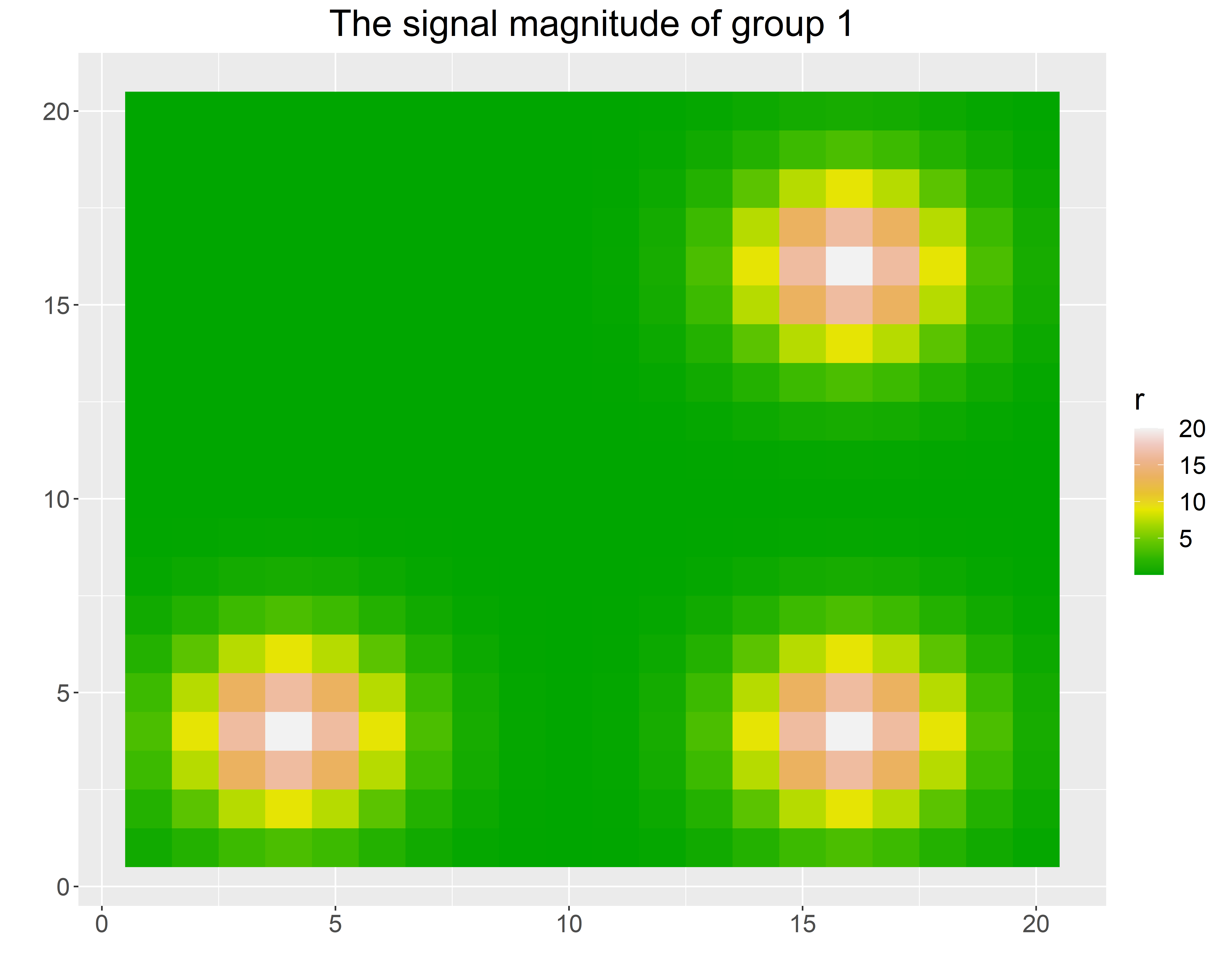
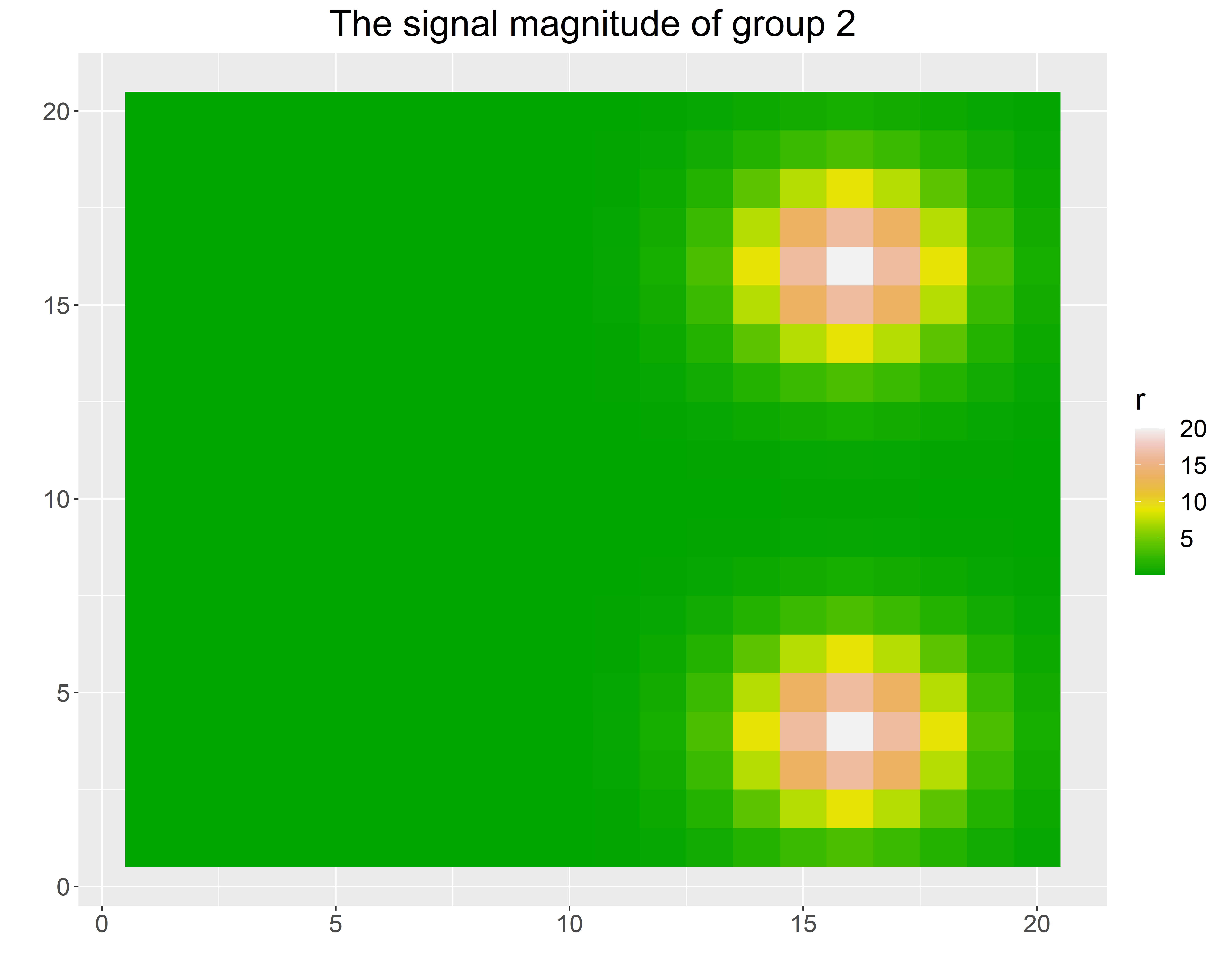
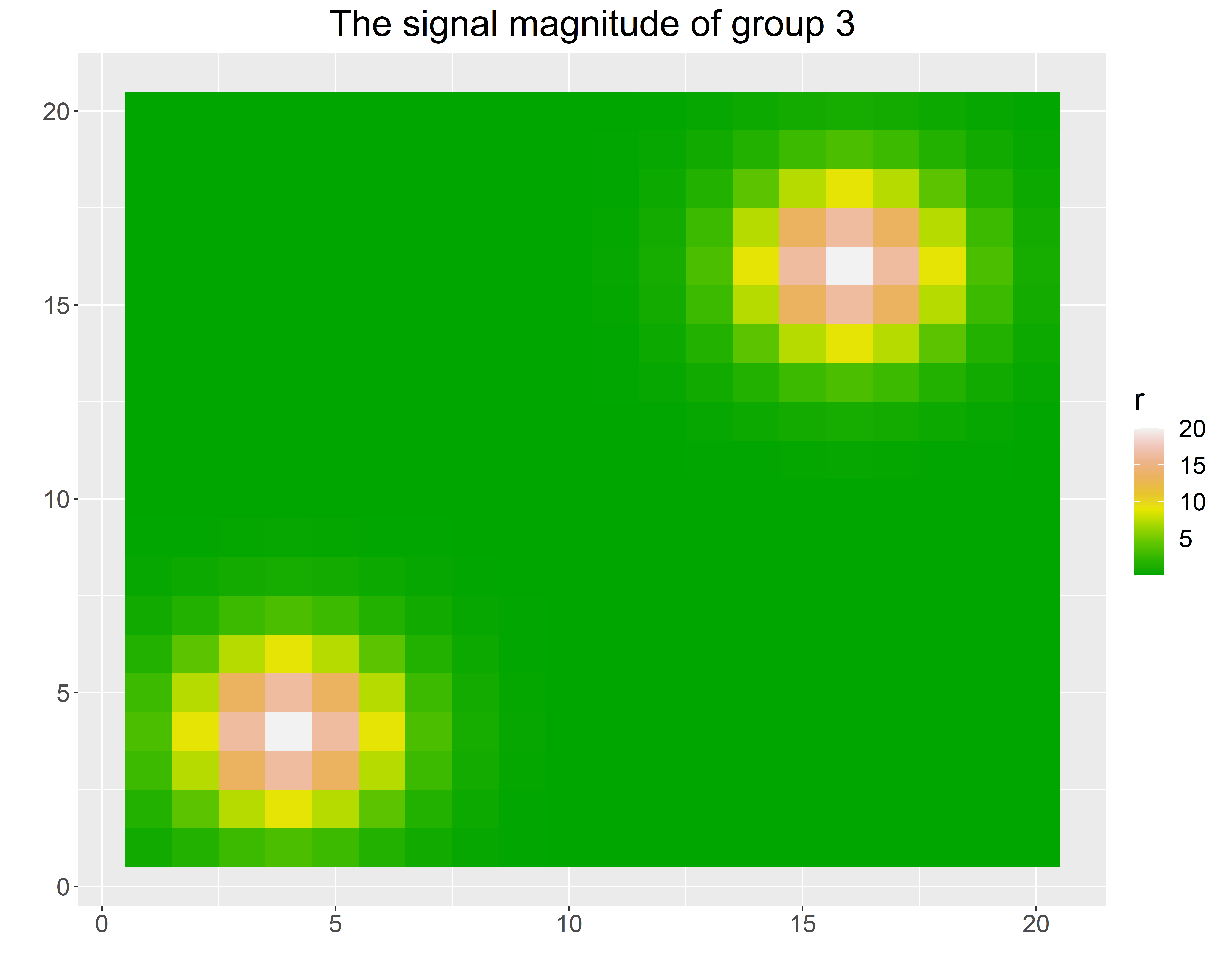
Figure 2: The magnitude $r_{g}$’s for different groups.

For our proposed Bayesian method, the choices of hyperparameters are $c_{1}=c_{2}=d_{1}=d_{2}=0.1$, $\sigma_{b}^{2}=10^{2},\nu=4,{\mathbf{S}}={\mathbf{I}}_{3}$ and $R=5$. Except for $R$, all the other choices of hyperparameters lead to weakly informative priors. The above choice of $R$ seems to work well both in simulations and real data applications. We collect 10000 MCMC samples and consider the last 5000 as post-burn-in samples for inferences. The other competing methods are not designed for vector-valued image predictors, nor in a multi-group setting. Hence, we consider $D_{i,1}({\mathbf{v}})$, $D_{i,2}({\mathbf{v}})$ and $D_{i,3}({\mathbf{v}})$ as three separate image predictors and fit the models for each group separately. We also compare our method with STGP, LASSO and functional principal component analysis (fPCA) (Jones and Rice, 1992) based on mean squared error $\frac{1}{3p}\sum_{j=1}^{p}\sum_{g=1}^{3}\|\hat{\mbox{\boldmath$\beta$}}_{g}({\mathbf{v}}_{j})-\mbox{\boldmath$\beta$}_{0,g}({\mathbf{v}}_{j})\|_{2}^{2}$. The fPCA estimates are obtained as follows. After smoothing the images using fbps function of refund package (refund), eigendecomposition of the sample covariance is computed. After that lasso regularized principal components regression is performed. The leading eigenvectors that explain 95% of the variation in the sample images are used to get the final estimate. glmnet is considered to fit the LASSO penalized regression model (friedman2017package). We also compare with group-LASSO and PING, which are not presented as their performances are similar to LASSO and STGP respectively.

5.1 Simulation case 1

In simulation case 1, the datasets are generated such that they closely mimic our real dataset on the principal diffusion direction of diffusion tensor imaging. The principal diffusion directions are unit vectors, and thus we rely on von Mises-Fisher distribution. We first generate mean fiber directions $\mbox{\boldmath$\eta$}_{{\mathbf{D}}}({\mathbf{v}})$’s. They are illustrated in panel (a) of Figure 3. Specifically, these mean directions maintain a spatial dependency pattern. Then we generate ${\mathbf{D}}_{i}({\mathbf{v}})$ as ${\mathbf{D}}_{i}({\mathbf{v}})\sim\textrm{vMF}(30,\mbox{\boldmath$\eta$}_{{\mathbf{D}}}({\mathbf{v}}))$ using R package Rfast (Papadakis et al., 2021) for each subject $i$ and each spatial location ${\mathbf{v}}$ on the above-mentioned grid. Here, vMF stands for the von Mises-Fisher distribution. Table 1 compares the estimated mean square error as defined earlier across different methods and Figure 4 illustrates the norms of estimated regression coefficients as well as the similar-effect locations using the F-values, defined below Lemma 4. All the methods perform better when the sample size increases or the error variance decreases. Our proposed ST2N-GP performs the best, indicating superiority of the proposed shrinkage prior in scalar on vector-valued image regression setting. The poorest performance of LASSO is probably because it fails to incorporate spatial dependence.

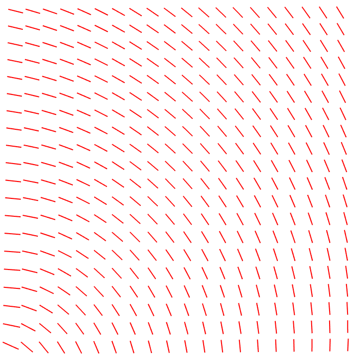
(a) The mean direction $(\mbox{\boldmath$\eta$}_{D}({\mathbf{v}}))$ to generate ${\mathbf{D}}_{i}({\mathbf{v}})$

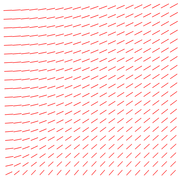
(b) Direction $\mbox{\boldmath$\eta$}({\mathbf{v}})$’s while constructing $\mbox{\boldmath$\beta$}_{0,g}$’s

Figure 3: The above shown directional unit are generated while sampling the predictors ${\mathbf{D}}_{i}({\mathbf{v}})$’s and constructing the coefficients $\mbox{\boldmath$\beta$}_{0,g}$’s.

Table 1: MSE of the vector-valued slope $\mbox{\boldmath$\beta$}({\mathbf{v}})$ when the predictors are generated as described in simulation case 1 with varying sample size and true error variance. There are total three groups with sample size as mentioned in the first column.

		Fitted Model
Group-specific	Error	ST2N-GP	STGP	LASSO	FPCA
sample size	variance
	1	0.62	0.89	6.85	1.64
50	5	0.88	1.19	6.20	1.54
	10	1.35	1.42	7.13	1.63
	1	0.28	0.44	4.27	1.26
100	5	0.37	0.98	4.36	1.43
	10	0.81	1.03	6.96	1.43

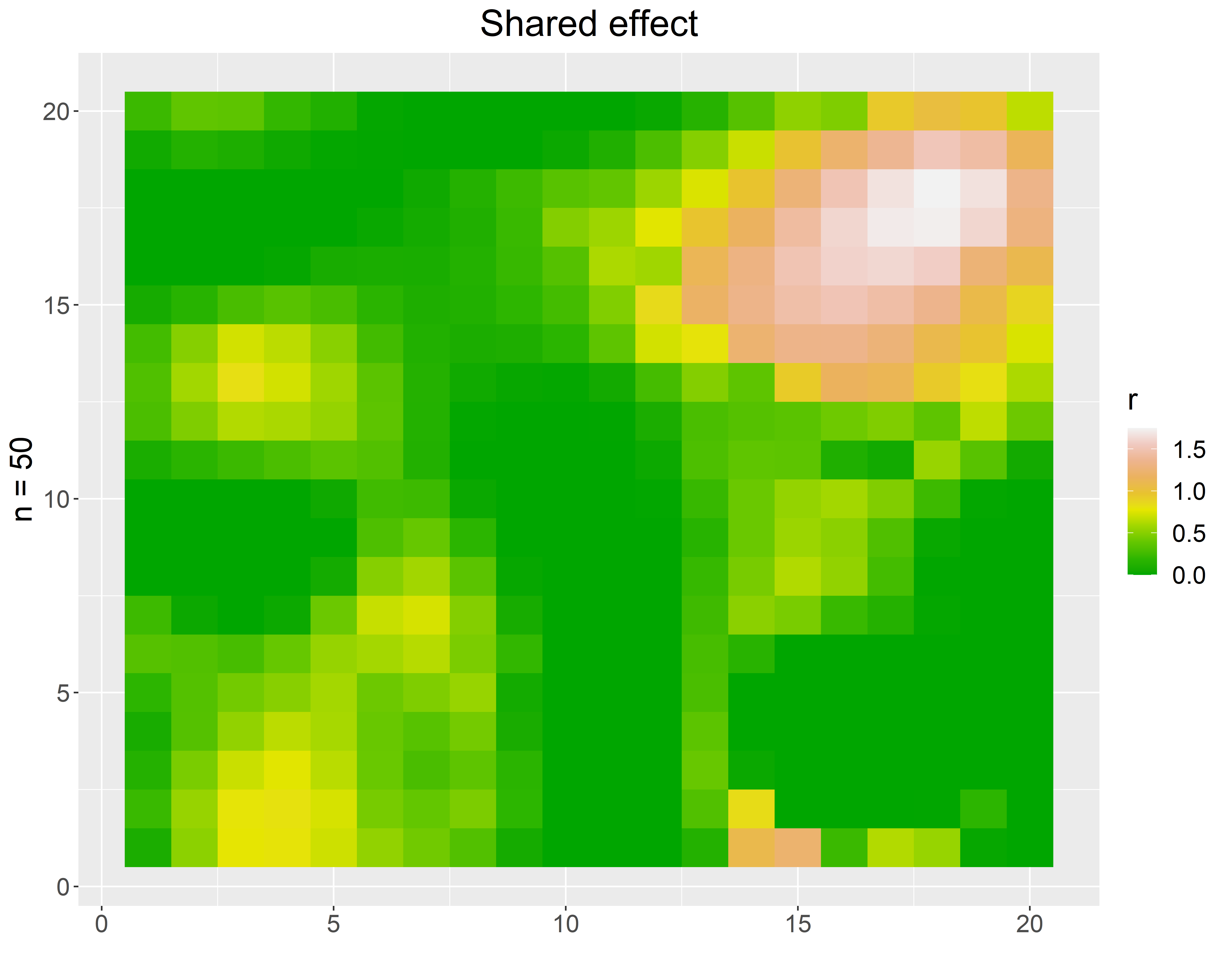
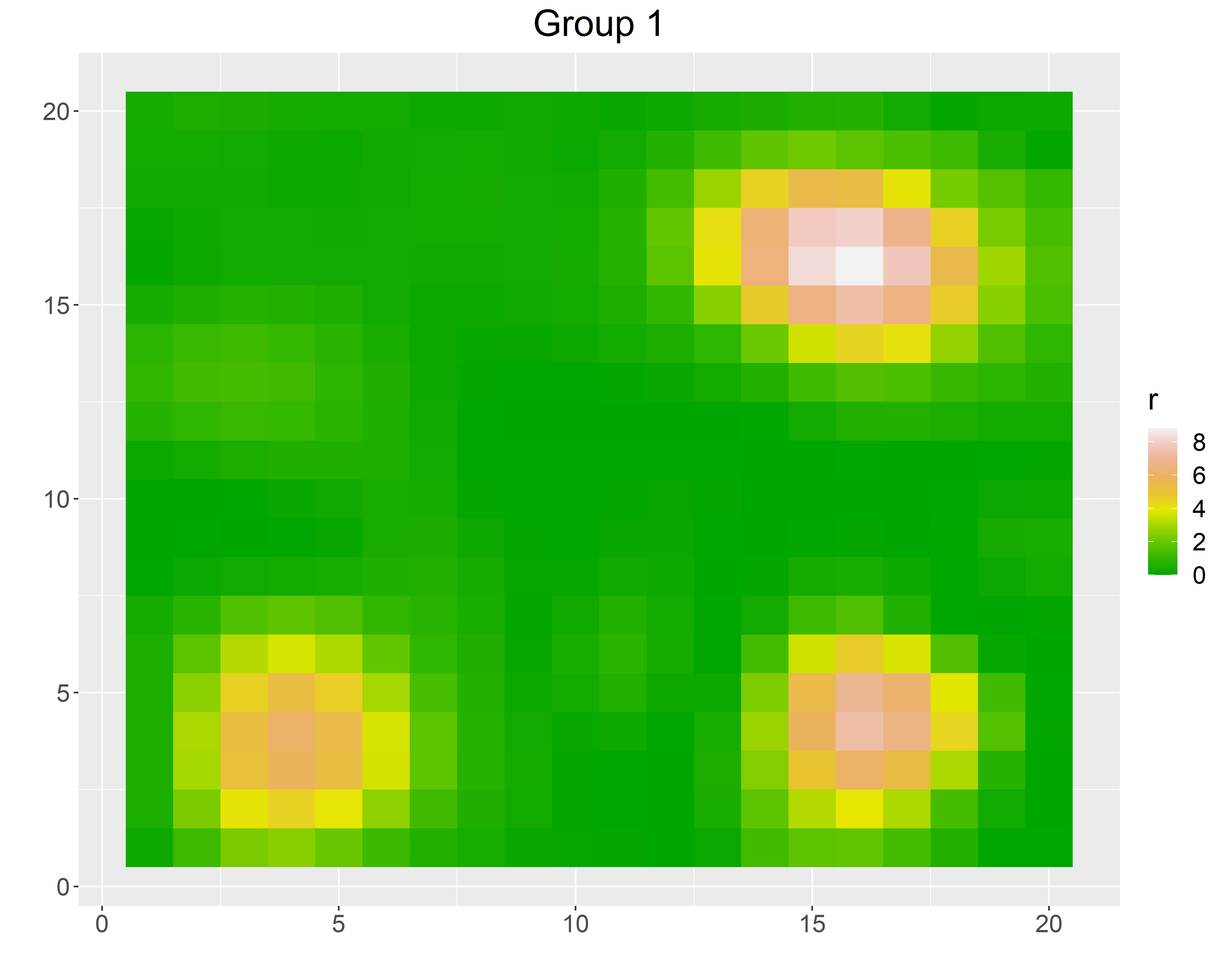
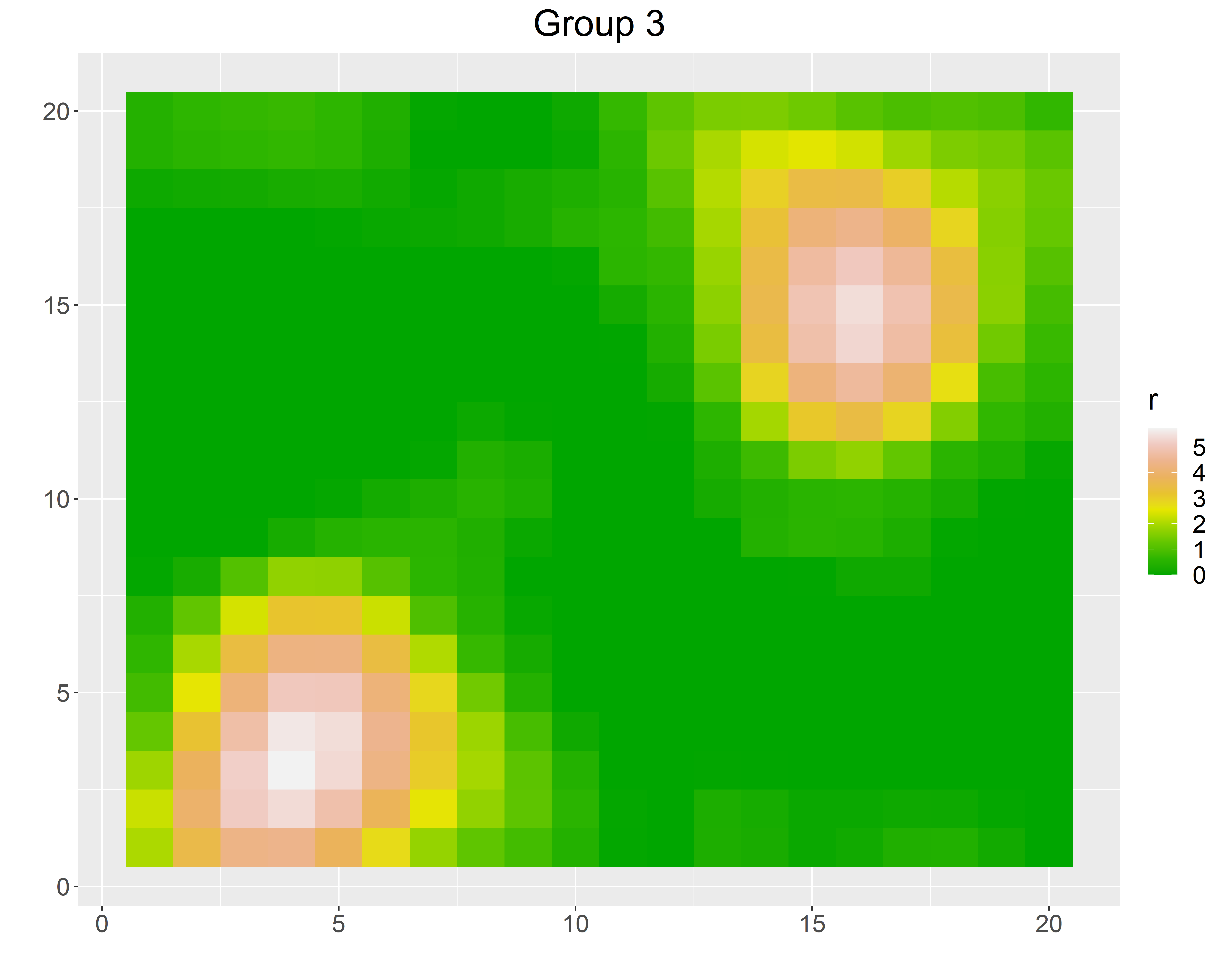
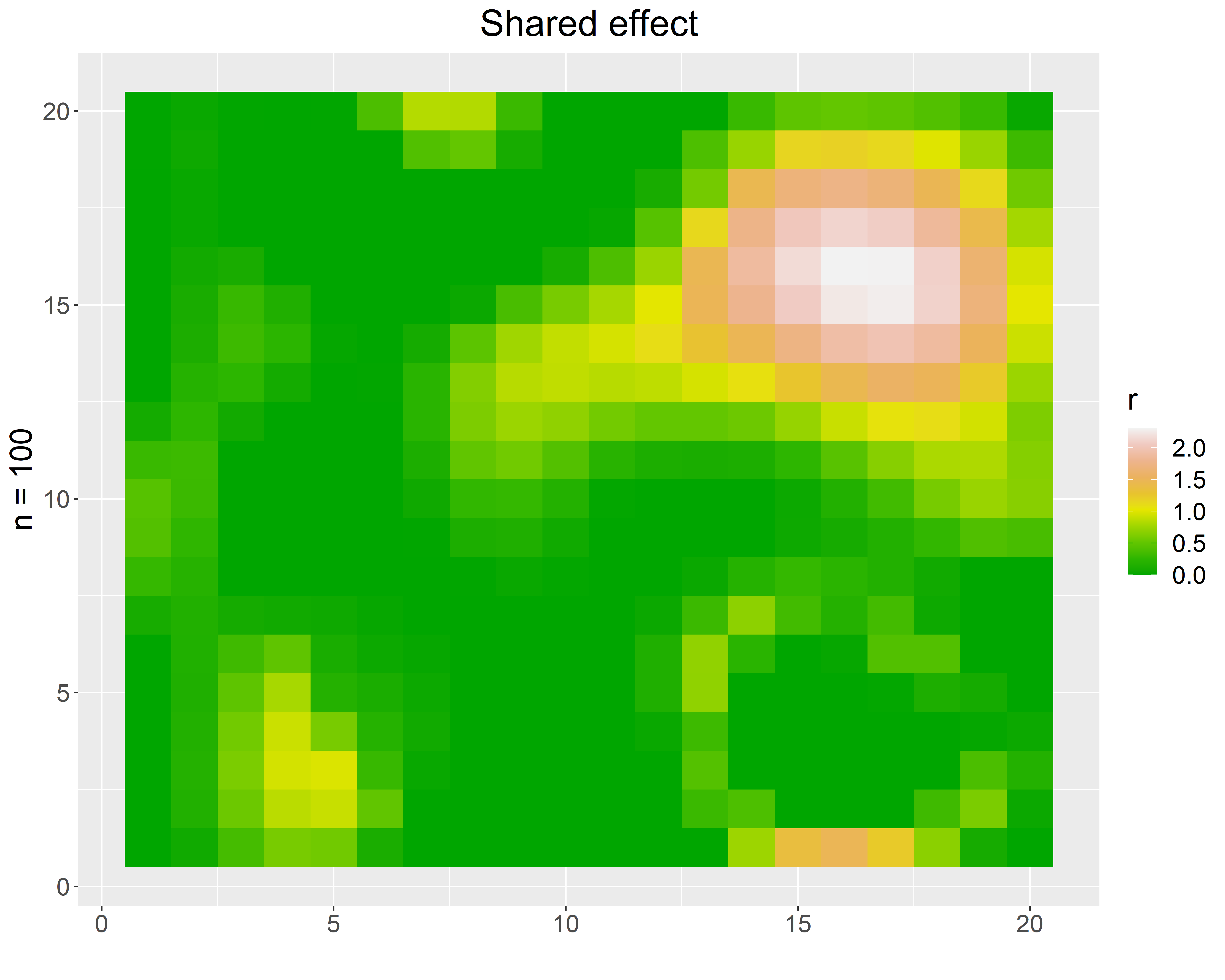
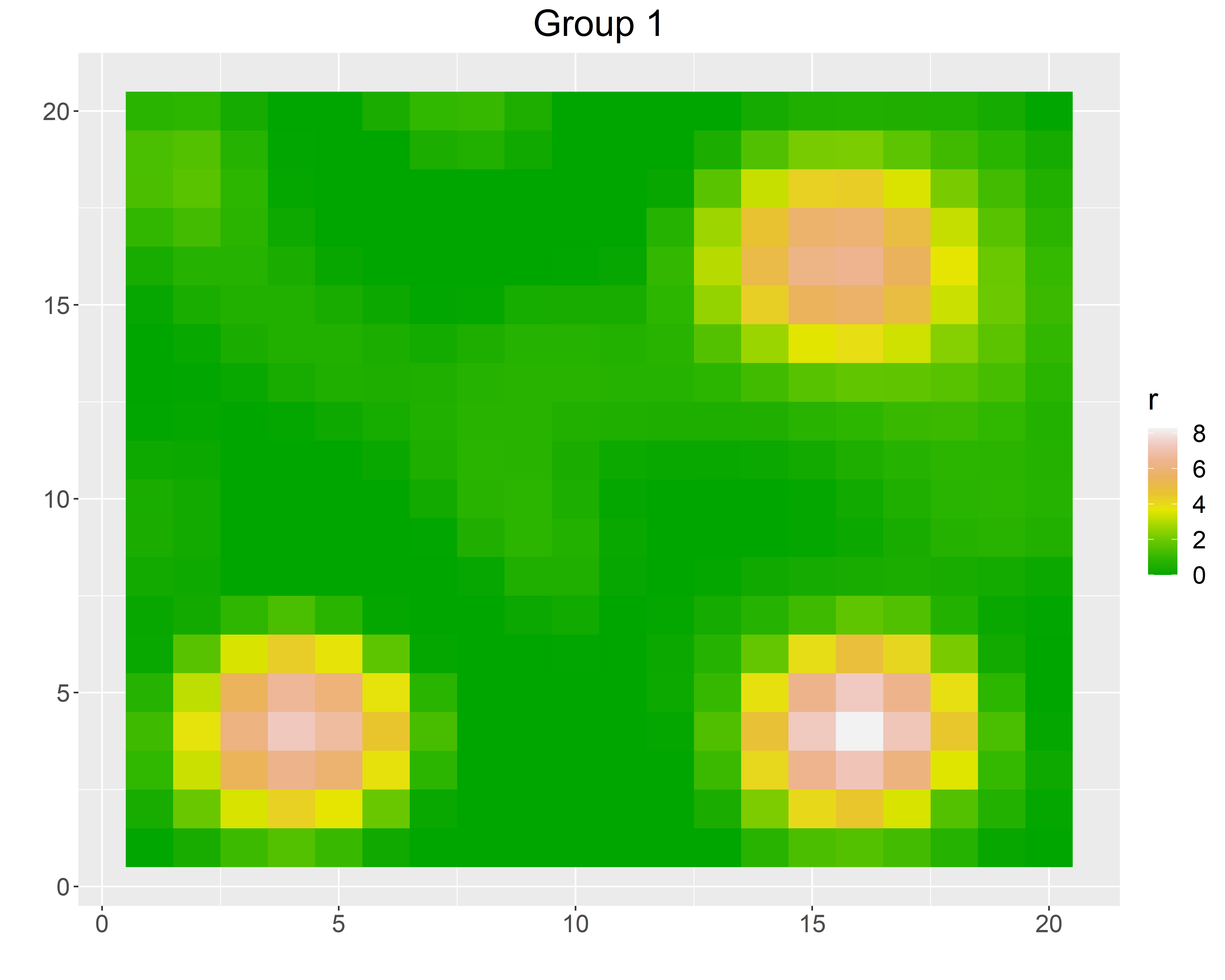
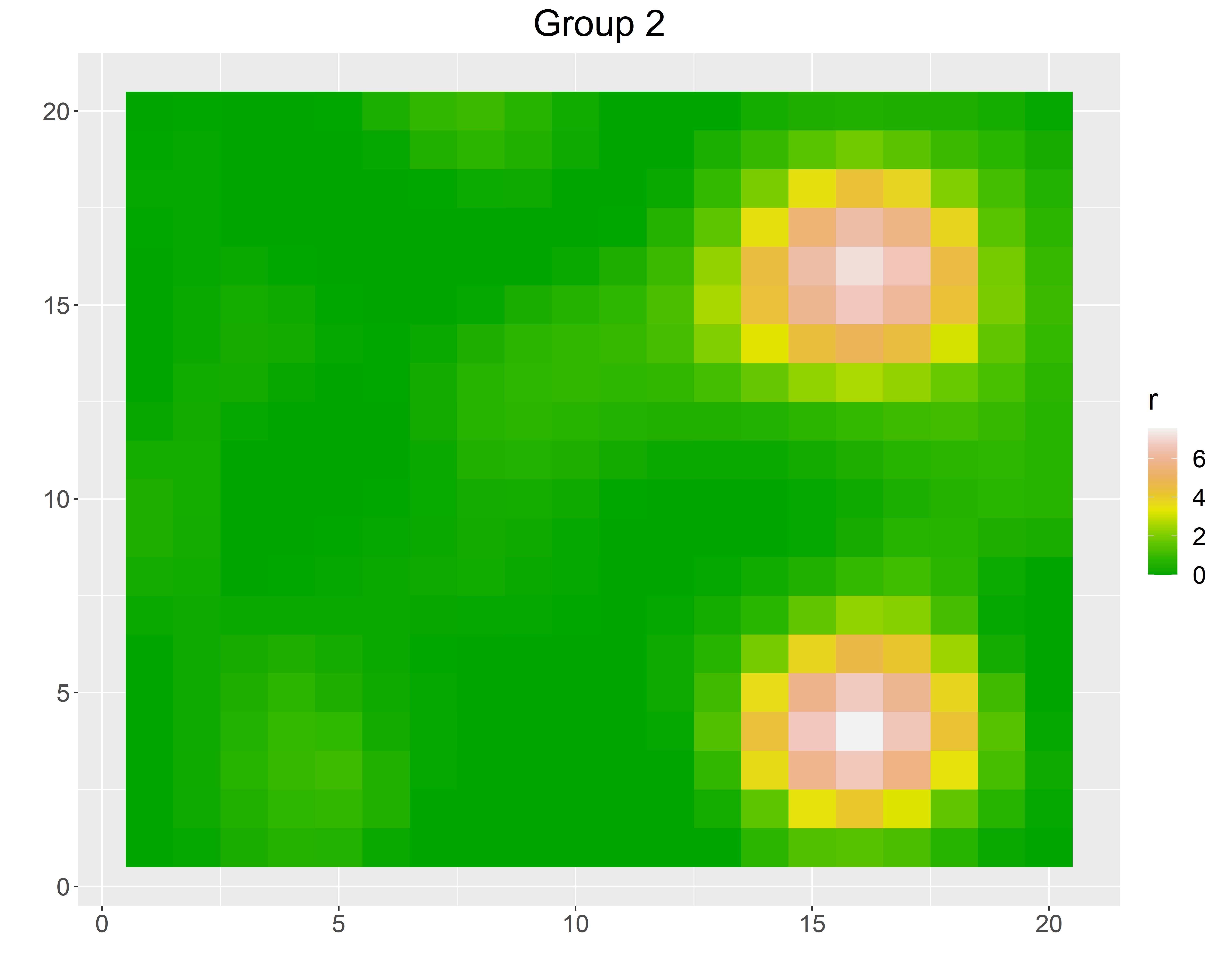
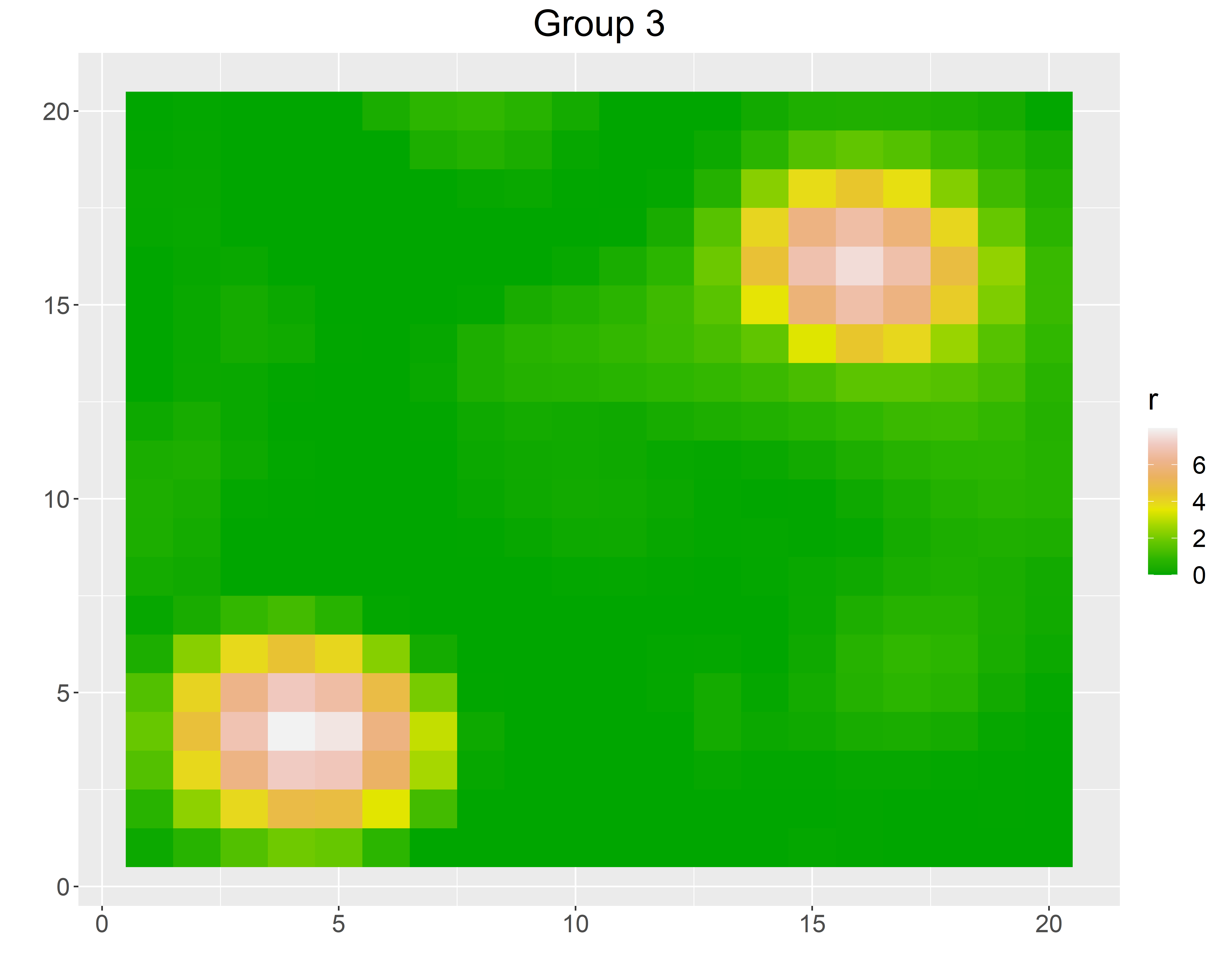
Figure 4: Estimated $\|F(h_{\lambda}(\widetilde{\mbox{\boldmath$\beta$}}))\|_{2}$ and $\|\mbox{\boldmath$\beta$}_{g}\|_{2}$’s when the error variance is $1$ for two sample sizes. The first row corresponds to sample size 50 in each group, and the second row is for 100.

5.2 Simulation case 2

The simulated datasets ${\mathbf{D}}_{i}({\mathbf{v}})$’s for this case are generated as follows. We first generate ${\mathbf{D}}^{\prime}_{i}({\mathbf{v}})=\{D_{i,1}^{\prime}({\mathbf{v}}),D_{i,2}^{\prime}({\mathbf{v}}),D_{i,3}^{\prime}({\mathbf{v}})\}$, following independent Gaussian processes with mean $\mathbb{E}(D_{i,1}^{\prime}({\mathbf{v}}))=\mathbb{E}(D_{i,2}^{\prime}({\mathbf{v}}))=\mathbb{E}(D_{i,3}^{\prime}({\mathbf{v}}))=0$ and exponential covariance kernels with different band widths, specifically, $\mathbb{E}(D_{i,1}^{\prime}({\mathbf{v}})D_{i,1}^{\prime}({\mathbf{v}}^{\prime}))=\exp(-\|{\mathbf{v}}-{\mathbf{v}}^{\prime}\|_{2}/3)$, $\mathbb{E}(D_{i,2}^{\prime}({\mathbf{v}})D_{i,2}^{\prime}({\mathbf{v}}^{\prime}))=\exp(-\|{\mathbf{v}}-{\mathbf{v}}^{\prime}\|_{2}/5)$, and $\mathbb{E}(D_{i,3}^{\prime}({\mathbf{v}})D_{i,3}^{\prime}({\mathbf{v}}^{\prime}))=\exp(-\|{\mathbf{v}}-{\mathbf{v}}^{\prime}\|_{2}/7)$. Finally, we generate a positive definite matrix $\Psi$ and set ${\mathbf{D}}_{i}({\mathbf{v}})=\mbox{\boldmath$\Psi$}{\mathbf{D}}_{i}^{\prime}({\mathbf{v}})$. Thus, marginally at each ${\mathbf{v}}$, we have $V\{{\mathbf{D}}_{i}({\mathbf{v}})\}=\mbox{\boldmath$\Psi$}\mbox{\boldmath$\Psi$}^{T}$.

Table 2: MSE of the vector-valued slope $\mbox{\boldmath$\beta$}({\mathbf{v}})$ when the predictors are generated as described in simulation case 2 with varying sample size and true error variance. There are total three groups with sample size as mentioned in the first column.

		Fitted Model
Group-specific	Error	ST2N-GP	STGP	LASSO	FPCA
sample size	variance
	1	0.11	0.28	10.57	0.90
50	5	0.12	0.34	10.45	0.87
	10	0.18	0.39	10.46	0.91
	1	0.05	0.12	2.69	0.87
100	5	0.05	0.12	2.70	0.87
	10	0.05	0.14	2.78	0.87

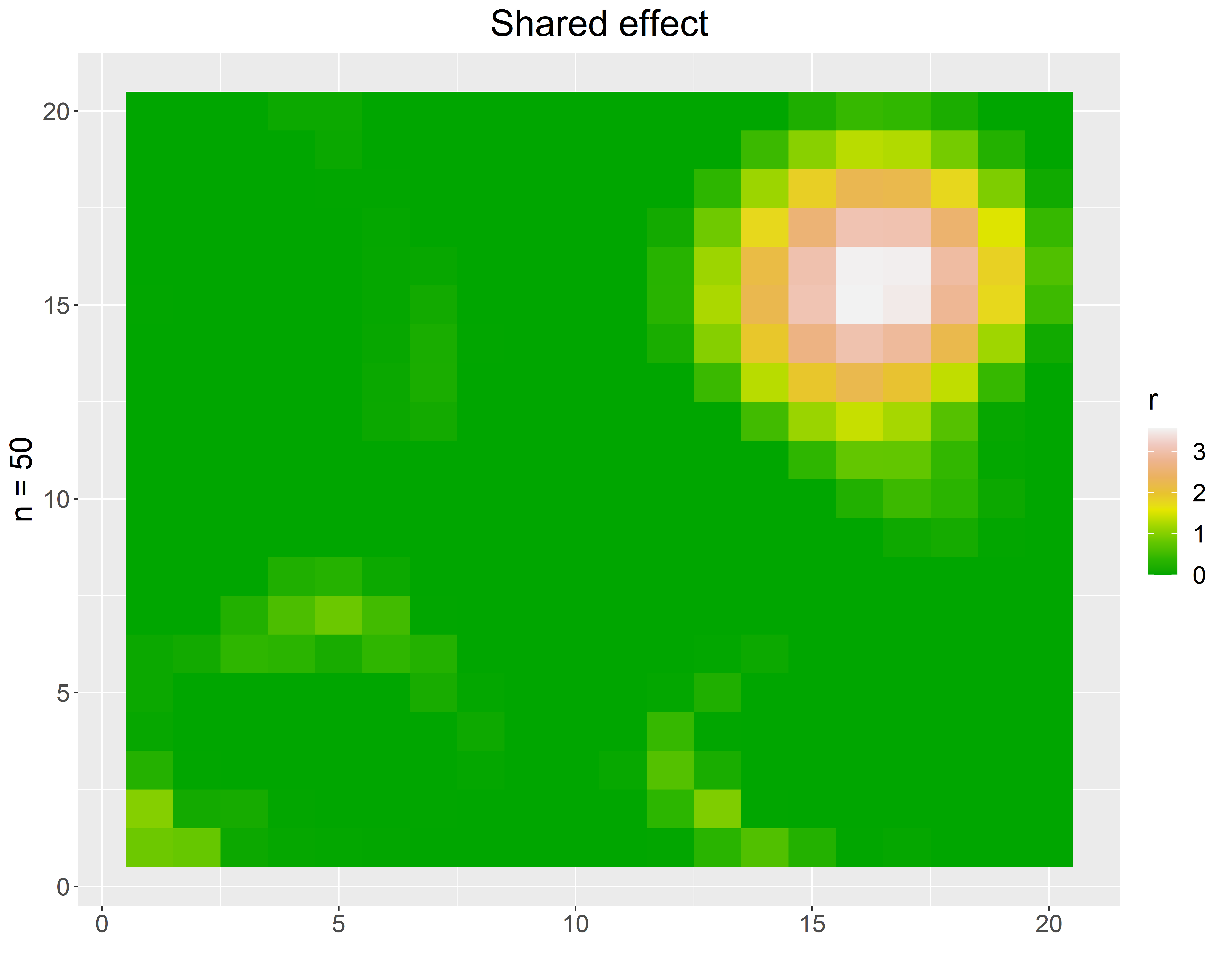
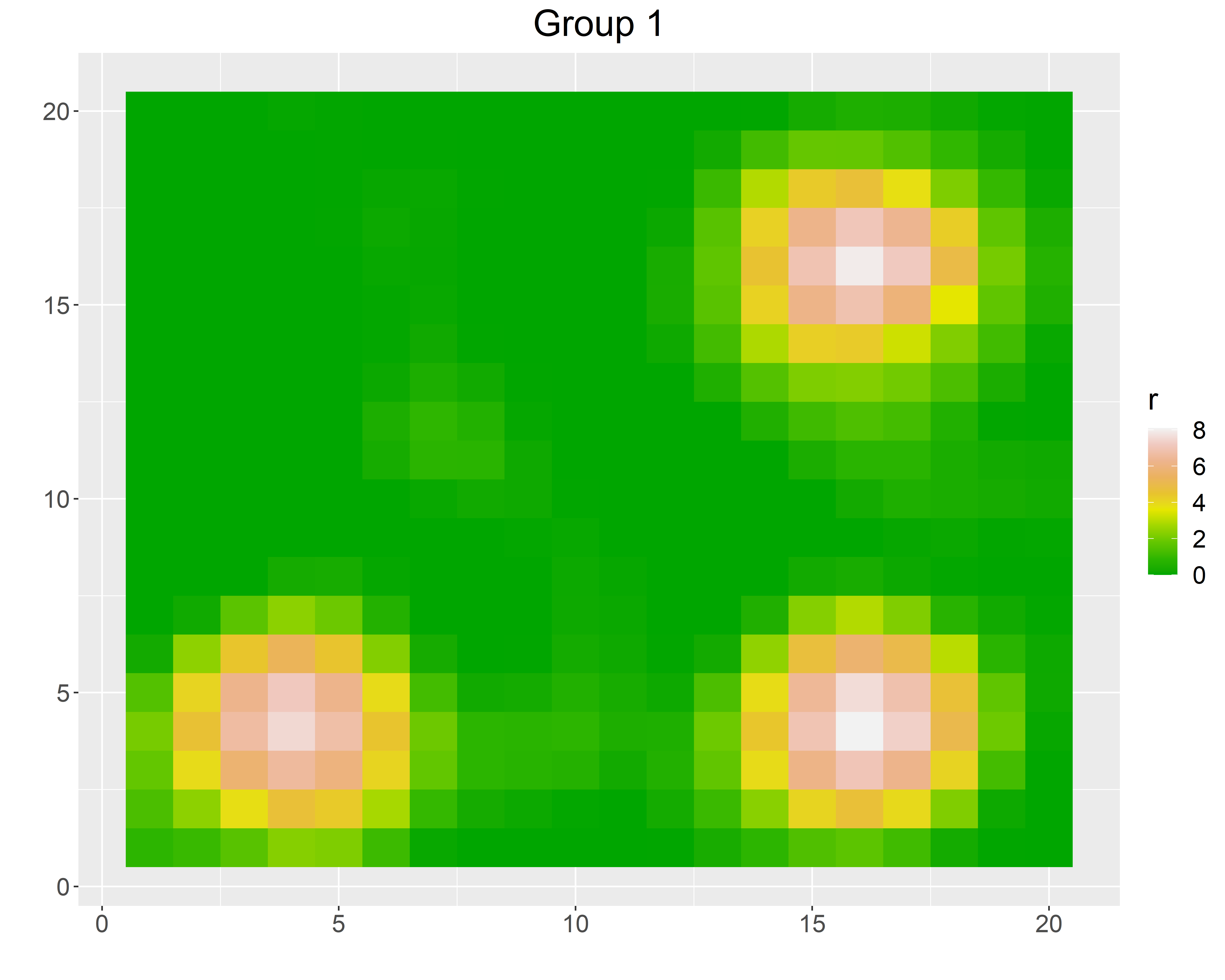
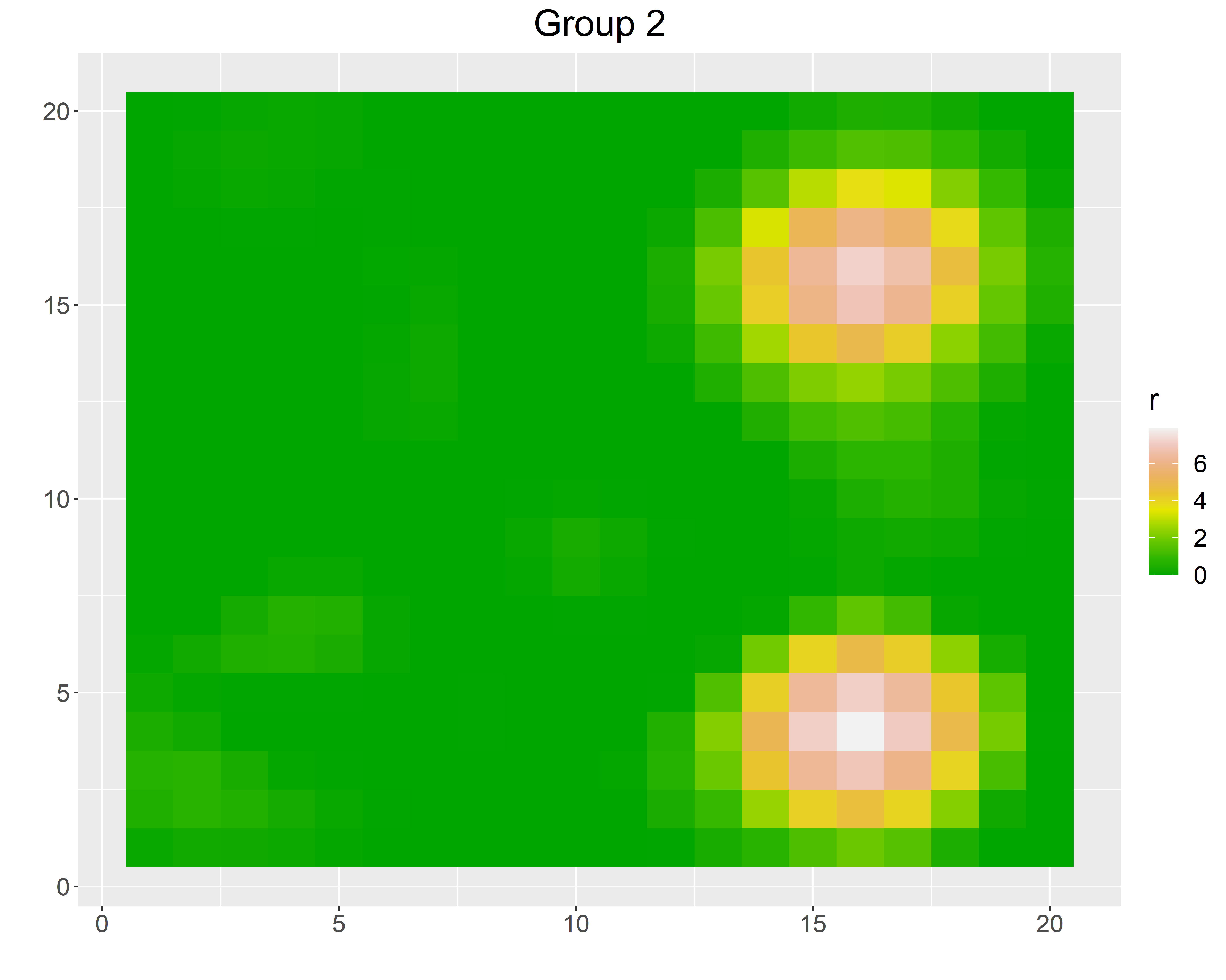
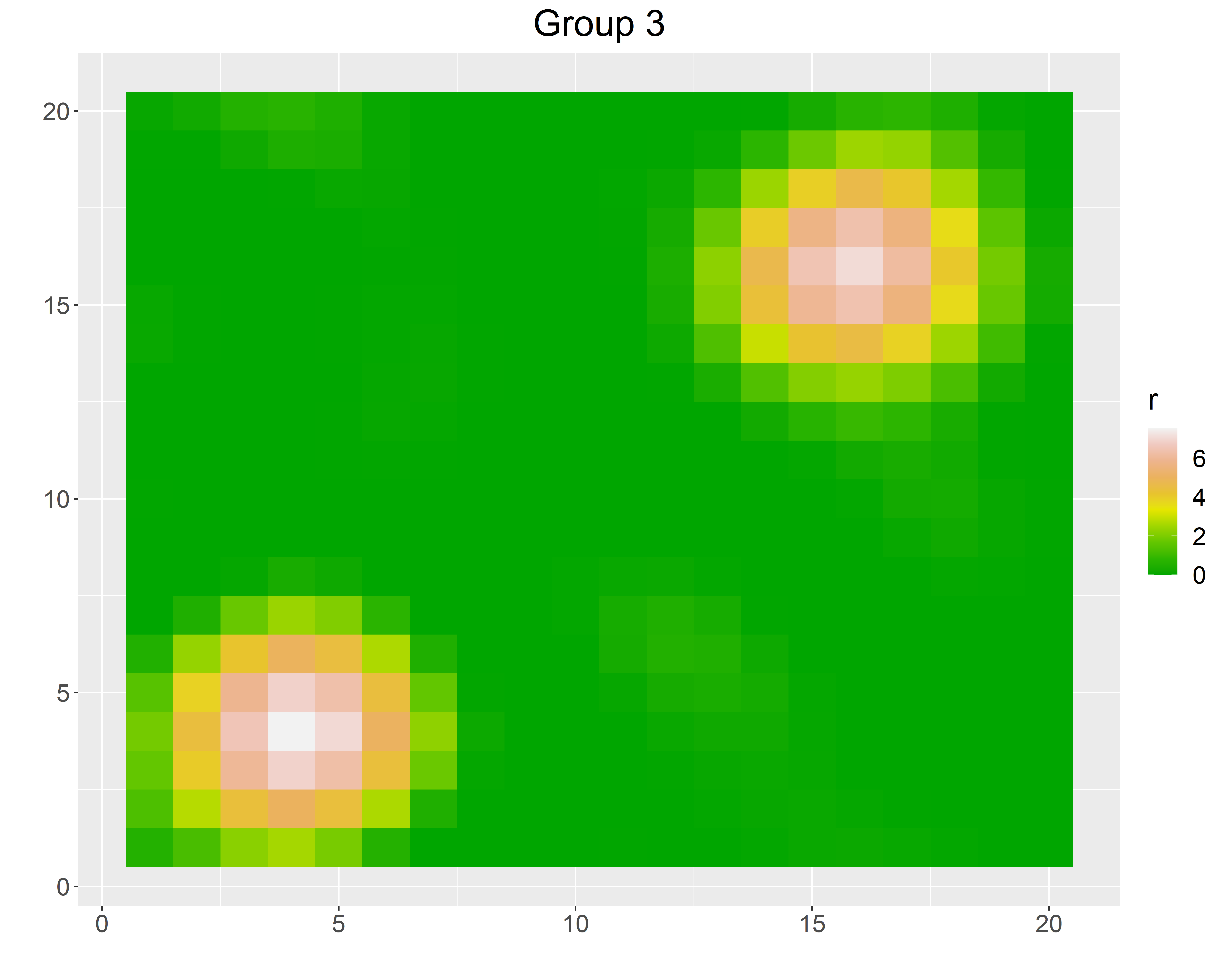
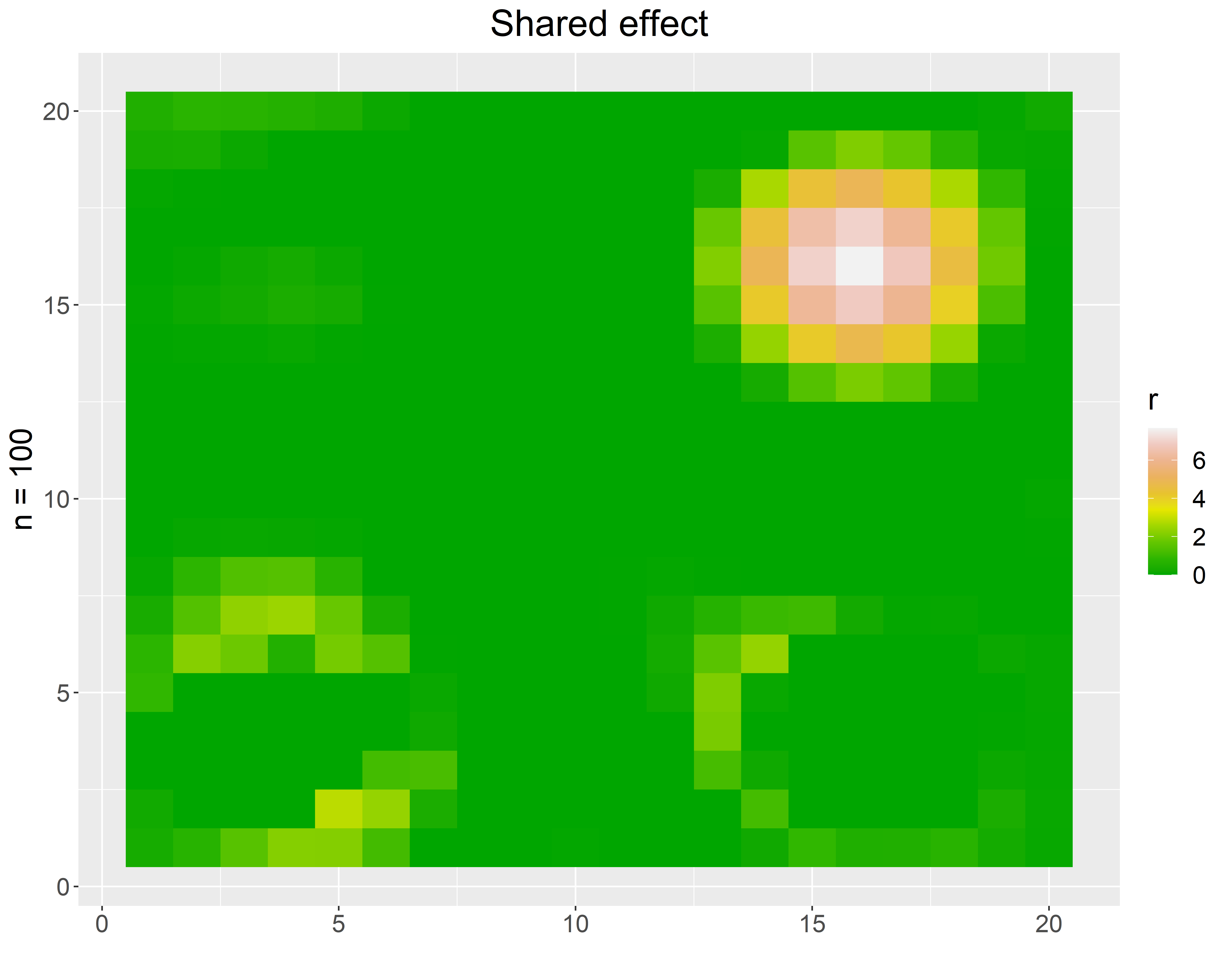
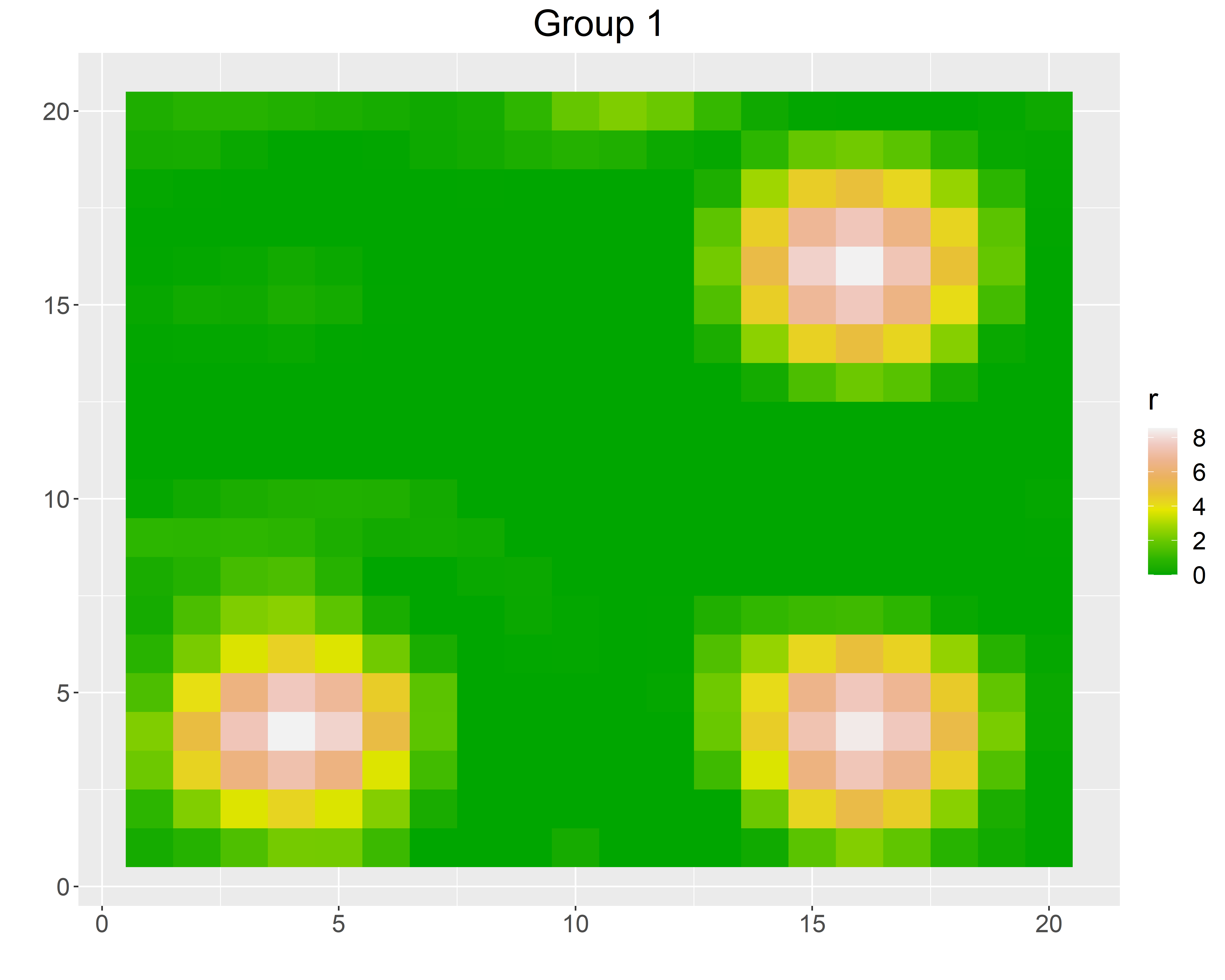
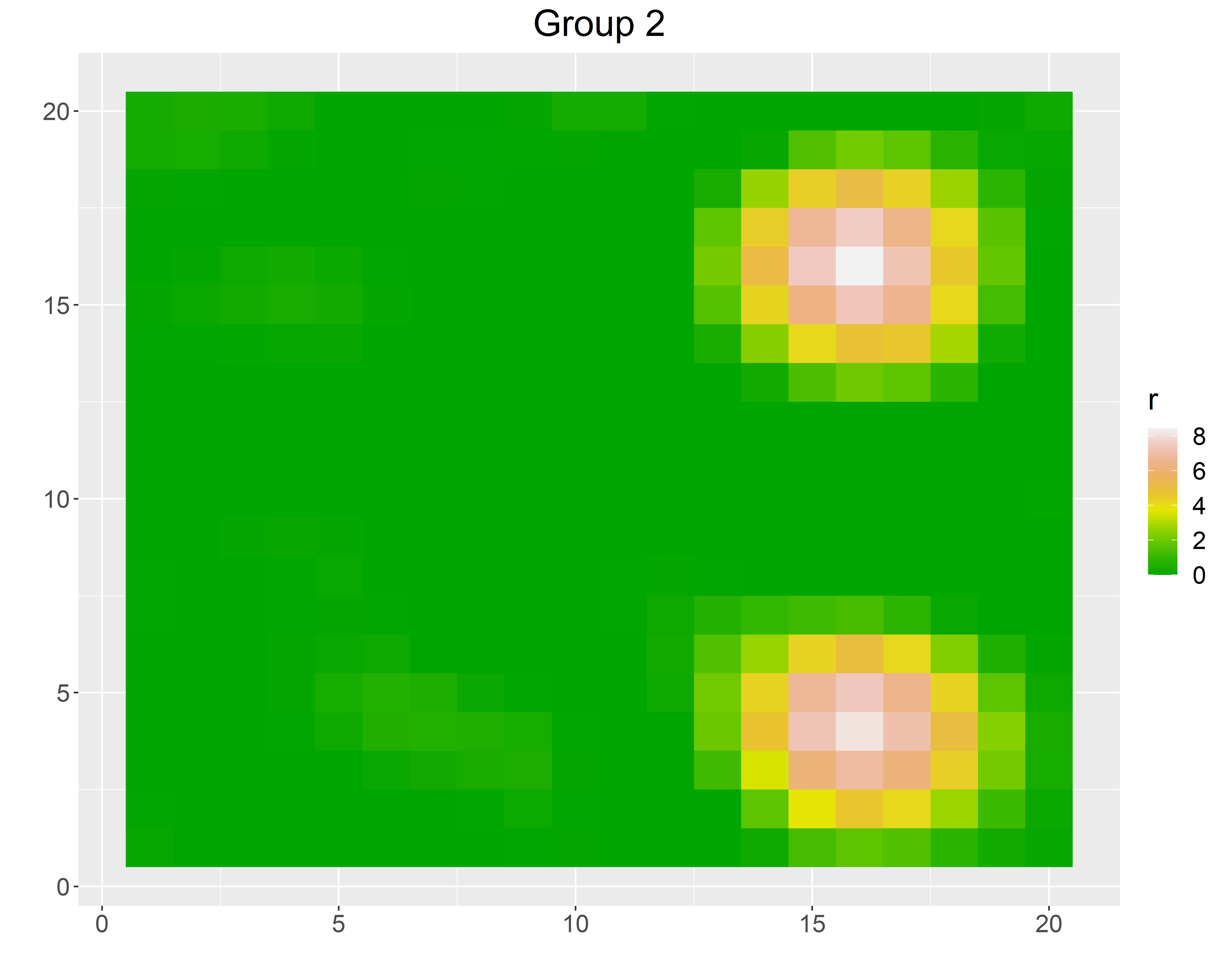
Figure 5: Estimated $\|F(h_{\lambda}(\widetilde{\mbox{\boldmath$\beta$}}))\|_{2}$ and $\|\mbox{\boldmath$\beta$}_{g}\|_{2}$’s when the error variance is $1$ for two sample sizes. The first row corresponds to sample size of 50 in each group, and the second row is for 100.

The performances of all the methods are compared in Table 2 and the norms of the estimated coefficients are shown in Figure 5. We again find that the proposed method is doing much better than all the other competitors. The poor performance of other methods may be primarily attributed to the dependence among the components in ${\mathbf{D}}_{i}$’s. With an increasing sample size and smaller error variance, all the methods perform much better as observed in case 1. Furthermore, the performances are usually better when the error variance is lower, which corresponds to a greater signal-to-noise ratio. Besides, for both of the two simulation cases, $\|F(h_{\lambda}(\widetilde{\mbox{\boldmath$\beta$}}))\|_{2}$’s accurately identify the similar-effect locations.

6 Application to the ADNI dataset

Data used in the preparation of this article were obtained from the Alzheimer’s Disease Neuroimaging Initiative (ADNI) database (adni.loni.usc.edu). The ADNI was launched in 2003 as a public-private partnership, led by Principal Investigator Michael W. Weiner, MD. The primary goal of ADNI has been to test whether serial magnetic resonance imaging (MRI), positron emission tomography (PET), other biological markers, and clinical and neuropsychological assessment can be combined to measure the progression of mild cognitive impairment (MCI) and early Alzheimer’s disease (AD). For up-to-date information, see www.adni-info.org.

We collect data belonging to three disease groups: Alzheimer’s disease, early and late mildly cognitive impaired (MCI) which are abbreviated as AD, EMCI, and LMCI for easy reference in the rest of the article. Several studies have established associations between gender, age, and APOE status with mini-mental state examination (MMSE) (Winnock et al., 2002; Qian et al., 2021; Matthews et al., 2012; Piccinin et al., 2013; Pradier et al., 2014). We thus apply our proposed model (1) after adjusting for these predictors. Our final model for the real data analysis is,

$${\textrm{MMSE}}_{i}= b_{0,g}+b_{\textrm{Age}}\textrm{Age}_{i}+b_{\textrm{M}}Z_{i,\textrm{Male}}$$

$$+b_{\textrm{Allele2}}Z_{\textrm{Allele2},i}+b_{\textrm{Allele4}}Z_{\textrm{Allele4},i}+p^{-1/2}\sum_{j=1}^{p}{\mathbf{D}}_{i}({\mathbf{v}}_{j})^{T}\mbox{\boldmath$\beta$}_{g}({\mathbf{v}}_{j})+e_{i},\textrm{ for }i\in g$$

$$e_{i}\sim \hbox{Normal}(0,\sigma^{2}),\quad g=\textrm{AD, EMCI, LMCI}$$ (3)

where the dummy variables $Z_{\text{APOE2}}$, $Z_{\textrm{APOE4}}$ standing for Alleles 3 and 4 for the two alleles APOEallele2 and APOEallele4 together setting Allele 3 as a reference group for each of the two cases. Similarly, the dummy variable $Z_{\textrm{M}}$ indicating male gender is introduced, setting females as the reference group. We put the ST2N-GP prior on $\mbox{\boldmath$\beta$}_{g}$’s.

While applying the model to the corresponding diffusion tensor data of the ADNI, we consider the principal diffusion direction as our predictor. It is represented by the first eigenvector of the diffusion coefficient matrices. Hence, ${\mathbf{D}}_{i}({\mathbf{v}})$’s are 3-dimensional unit vectors. In our modeling framework, we thus have ${\mathbf{D}}_{i}({\mathbf{v}})^{T}\mbox{\boldmath$\beta$}({\mathbf{v}})=\|\mbox{\boldmath$\beta$}({\mathbf{v}})\|_{2}\cos(\theta_{{\mathbf{D}}_{i}({\mathbf{v}}),\mbox{\boldmath$\beta$}({\mathbf{v}})})$. Hence, $\|\mbox{\boldmath$\beta$}({\mathbf{v}})\|_{2}$ now represents overall magnitude of effect from voxel ${\mathbf{v}}$ and $\theta_{{\mathbf{D}}_{i}({\mathbf{v}}),\mbox{\boldmath$\beta$}({\mathbf{v}})}$ stands for individual specific direction of effect.

Figure 6 illustrates the important regions for different brain regions. In our estimates, we observe the following interesting characteristics. Estimates associated with the EMCI group usually have the largest number of important regions, then LMCI, and lastly AD with the smallest number of selected regions. The lower part of each tract has a greater number of important areas. This may be due to the higher white matter density of that part. Corpus callosum has the maximum percentage of important regions, which may also be attributed to the greater density of white matter. In Table 4, gender turns out to be important for all the cases, and age has an important negative effect in the two cases. The uneven proportion of important regions for different disease groups justifies our multi-group model with group-specific regression effects. The effect of APOE4 turns out to be significant only for corpus callosum. At most of the similar-effect locations, the $\psi({\mathbf{v}})$’s (defined in Section 2.2) turn out to be very high, implying very strong across-group similarities at the similar-effect locations. There are several interesting findings in our analysis using the white matter fiber alignment directly. Our follow-up future analyses will consider other DTI markers too.

Table 3: Estimated effects of different scalar predictors. In the first column, the region names are provided. For each predictor, we report the posterior mean along with its lower and upper credible bands.

		Gender	Age	Allele 3	Allele 4
	Estimate	1.36	-0.40	0.94	-0.66
Corpus Callosum	Lower CI	0.62	-0.76	-0.84	-1.37
	Upper CI	2.15	-0.06	2.62	-0.01
	Estimate	0.96	-0.10	0.77	0.64
Right CST	Lower CI	0.23	-0.49	-0.80	-0.39
	Upper CI	1.70	0.25	2.27	1.53
	Estimate	1.06	-0.19	1.11	0.00
Left CST	Lower CI	0.36	-0.52	-0.27	-0.74
	Upper CI	1.72	0.13	2.47	0.97
	Estimate	1.43	-0.51	1.18	0.12
Right FPT	Lower CI	0.69	-0.88	-0.48	-0.66
	Upper CI	2.23	-0.12	2.77	0.89
	Estimate	0.96	-0.07	1.23	0.18
Left FPT	Lower CI	0.29	-0.44	-0.23	-0.62
	Upper CI	1.65	0.32	2.77	0.96

(a) Shared CC (4.48%)

(b) AD CC (6.68%)

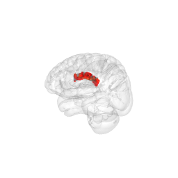
(c) EMCI CC (9.94%)

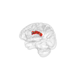
(d) LMCI CC (8.28%)

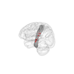
(e) Shared L. CST (2.55%)

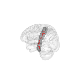
(f) AD L. CST (3.13%)

(g) EMCI L. CST (6.55%)

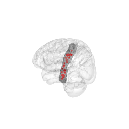
(h) LMCI L. CST (5.52%)

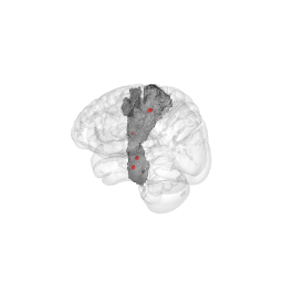
(i) Shared R. CST (1.13%)

(j) AD R. CST (2.55%)

(k) EMCI R. CST (11.29%)

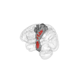
(l) LMCI R. CST (8.11%)

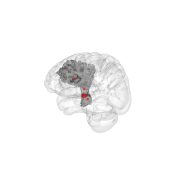
(m) Shared L. FPT (1.00%)

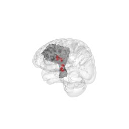
(n) AD L. FPT (2.87%)

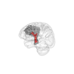
(o) EMCI L. FPT (14.05%)

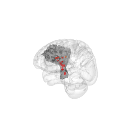
(p) LMCI L. FPT (4.27%)

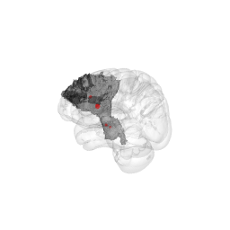
(q) Shared R. FPT (1.16%)

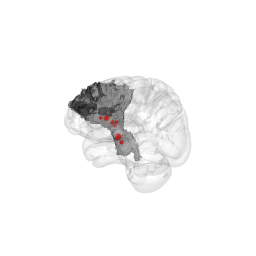
(r) AD R. FPT (3.11%)

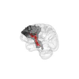
(s) EMCI R. FPT (12.76%)

(t) LMCI R. FPT (11.01%)

Figure 6: Estimated $\|F(h_{\lambda}(\widetilde{\mbox{\boldmath$\beta$}}))\|_{2}$ and $\|\mbox{\boldmath$\beta$}_{g}\|_{2}$’s for different brain masks along the percentage of non-zero voxels in the bracket.

We also compare ST2N with STGP in terms of out of sample prediction. STGP is chosen as a competitor since it was the second-best performer in the simulation after ST2N in estimating the true regression coefficient. The available code for STGP only allows to have imaging predictors. For a fair comparison, we thus consider a reduced model with only vector-valued DTI image as predictor and MMSE as response. As in Section 5, we apply STGP for each group separately and consider each coordinate of principal diffusion direction data as separate imaging predictor. For each group, we leave out 5 subjects and run the models with the rest of the subjects. ST2N overwhelmingly outperforms STGP. The poor performance of STGP may be due to group-specific separate estimation with small sample sizes. On the other hand, our multi-group model fits the three regression coefficient simultaneously. Hence, for multi-group data, our proposed model is more suitable.

Table 4: Out of sample prediction MSE, averaged over all the three groups for different brain masks.

	Corpus Callosum	Right CST	Left CST	Right FPT	Left FPT
ST2N	53.92	35.28	117.35	38.43	143.74
STGP	745.73	746.83	744.43	722.63	725.34

7 Discussion

In this paper, we developed a novel spatial variable selection prior for the vector-valued image on scalar regression. We further extended the model for the multi-group setting and implemented an efficient MCMC algorithm. The utility of the proposed method was demonstrated in a DTI data application. Methodologically, our proposed prior can be easily applied to a sparse nonparametric additive scalar on image regression model, which maybe formulated as, $y_{i}\sim\hbox{Normal}\left(\sum_{{\mathbf{v}}\in\mathcal{V}}\eta({\mathbf{v}})f_{{\mathbf{v}}}(x_{i}({\mathbf{v}})),\sigma^{2}\right)$. It is possible to rewrite the mean as $\sum_{{\mathbf{v}}\in\mathcal{V}}\eta({\mathbf{v}})f_{{\mathbf{v}}}(x_{i}({\mathbf{v}}))=\sum_{{\mathbf{v}}\in\mathcal{V}}\mbox{\boldmath$\beta$}({\mathbf{v}})^{T}{\mathbf{D}}_{i}({\mathbf{v}})$, where ${\mathbf{D}}_{i}({\mathbf{v}})=\{B_{k}(x_{i}({\mathbf{v}}))\}_{k=1}^{K}$ and $\mbox{\boldmath$\beta$}({\mathbf{v}})=\{\eta({\mathbf{v}})\theta_{k}({\mathbf{v}})\}_{k=1}^{K}$. Since $\eta({\mathbf{v}})$ and $\theta_{k}({\mathbf{v}})$ are not separately identifiable, we may directly put our ST2N-GP prior on $\mbox{\boldmath$\beta$}({\mathbf{v}})$ for spatial variable selection. Extension to such a modeling framework will be very useful for building a nonparametric regression model with an imaging predictor. Besides, these models are easier to interpret than the fully nonparametric version, as discussed in Ravikumar et al. (2009).

In the case of multimodal imaging, the predictor vector ${\mathbf{D}}_{i}({\mathbf{v}})$ may consist of both the main effects and the interaction effect terms, and we can analyze with the ST2N-GP prior. In our ADNI application, it will be interesting to add other imaging markers, derived from fMRI or PET, and run a combined multimodal analysis. The scaled squared exponential kernel can be replaced by more flexible Matérn kernel too. Furthermore, the latent process $\widetilde{\mbox{\boldmath$\beta$}}$ does not necessarily need to be a GP. It might follow newly proposed processes, such as Nearest Neighbor GP which is computationally more affordable than traditional GP. The latent process may even be modeled using the deep neural net, RBF-net, or any other flexible classes. In the future, we explore these possibilities too.

The ST2N transformation-based priors can be easily applied to the other types of vector-valued image regression models, where we may even have the image data as a response instead of being a predictor. Our future works will focus on such applications. Furthermore, we rerun our real data model for other DTI markers and compare our results to obtain better clarity. Future works will also pursue the possibilities to induce the spatial correlation in $\mbox{\boldmath$\beta$}_{g}$’s along the fiber tracts. We have also established the theoretical results under a completely new set of assumptions on the predictor process. Our assumptions are motivated by the developments in covariance matrix estimations theory. Hence, our theoretical results combine the two independently developed theories. Such characterization may help establish theoretical properties for other statistical models with spatially varying predictors. However, additional control on the predictor process might help us to establish even stronger posterior contraction and variable selection results.

8 Acknowledgments

Data collection and sharing for this project was funded by the Alzheimer’s Disease Neuroimaging Initiative (ADNI) (National Institutes of Health Grant U01 AG024904) and DOD ADNI (Department of Defense award number W81XWH-12-2-0012). ADNI is funded by the National Institute on Aging, the National Institute of Biomedical Imaging and Bioengineering, and through generous contributions from the following: AbbVie, Alzheimer’s Association; Alzheimer’s Drug Discovery Foundation; Araclon Biotech; BioClinica, Inc.; Biogen; Bristol-Myers Squibb Company; CereSpir, Inc.; Cogstate; Eisai Inc.; Elan Pharmaceuticals, Inc.; Eli Lilly and Company; EuroImmun; F. Hoffmann-La Roche Ltd and its affiliated company Genentech, Inc.; Fujirebio; GE Healthcare; IXICO Ltd.; Janssen Alzheimer’s Immunotherapy Research & Development, LLC.; Johnson & Johnson Pharmaceutical Research & Development LLC.; Lumosity; Lundbeck; Merck & Co., Inc.; Meso Scale Diagnostics, LLC.; NeuroRx Research; Neurotrack Technologies; Novartis Pharmaceuticals Corporation; Pfizer Inc.; Piramal Imaging; Servier; Takeda Pharmaceutical Company; and Transition Therapeutics. The Canadian Institutes of Health Research is providing funds to support ADNI clinical sites in Canada. Private sector contributions are facilitated by the Foundation for the National Institutes of Health (www.fnih.org). The grantee organization is the Northern California Institute for Research and Education, and the study is coordinated by the Alzheimer’s Therapeutic Research Institute at the University of Southern California. ADNI data are disseminated by the Laboratory for Neuro Imaging at the University of Southern California.

Appendix

Proof of Lemma 1.

We show the above result under the $\ell_{2}$ and $\ell_{\infty}$ norms as that will immediately help in our other theoretical results. Specifically, we show $\|h_{\lambda}({\mathbf{x}}_{1})-h_{\lambda}({\mathbf{x}}_{2})\|_{2}\leq\|{\mathbf{x}}_{1}-{\mathbf{x}}_{2}\|_{2}$ and $\|h_{\lambda}({\mathbf{x}}_{1})-h_{\lambda}({\mathbf{x}}_{2})\|_{\infty}\leq\|{\mathbf{x}}_{1}-{\mathbf{x}}_{2}\|_{\infty}$. We distribute the proof into three disjoint cases. Let ${\cal S}^{q-1}$ stands for the sphere with radius $\lambda$ around the origin.

Case 1: $\|{\mathbf{x}}_{1}\|_{2},\|{\mathbf{x}}_{2}\|_{2}\leq\lambda$, we have $\|h_{\lambda}({\mathbf{x}}_{1})-h_{\lambda}({\mathbf{x}}_{2})\|_{2}=0\leq\|{\mathbf{x}}_{1}-{\mathbf{x}}_{2}\|_{2}$.

Case 2: $\|{\mathbf{x}}_{1}\|_{2}\geq\lambda,\|{\mathbf{x}}_{2}\|_{2}\leq\lambda$, We have $\|h_{\lambda}({\mathbf{x}}_{1})-h_{\lambda}({\mathbf{x}}_{2})\|_{2}=\|h_{\lambda}({\mathbf{x}}_{1})\|_{2}=\|{\mathbf{x}}_{1}\|_{2}-\lambda$.

We have $\|{\mathbf{x}}_{1}-{\mathbf{x}}_{2}\|_{2}\geq\big{\|}{\mathbf{x}}_{1}-\|{\mathbf{x}}_{2}\|_{2}\frac{{\mathbf{x}}_{1}}{\|{\mathbf{x}}_{1}\|_{2}}\big{\|}_{2}$ by Cauchy–Schwarz inequality which gives us $(\sum_{i}{x_{1,i}^{2}})(\sum_{i}{x_{1,i}^{2}})\geq(\sum_{i}x_{1,i}x_{2,i})^{2}$. Since $\|{\mathbf{x}}_{2}\|_{2}<\lambda$, we have $\big{\|}{\mathbf{x}}_{1}-\|{\mathbf{x}}_{2}\|_{2}\frac{{\mathbf{x}}_{1}}{\|{\mathbf{x}}_{1}\|_{2}}\big{\|}_{2}>\big{\|}{\mathbf{x}}_{1}\|_{2}-\lambda$.

Case 3: $\|{\mathbf{x}}_{1}\|_{2}\geq\lambda,\|{\mathbf{x}}_{2}\|_{2}\geq\lambda$,

$$\|{\mathbf{x}}_{1}-{\mathbf{x}}_{2}\|^{2}_{2}-\|h_{\lambda}({\mathbf{x}}_{1})-h_{\lambda}({\mathbf{x}}_{2})\|^{2}_{2}\geq 2\lambda+2<h_{\lambda}({\mathbf{x}}_{1}),h_{\lambda}({\mathbf{x}}_{2})>-2<{\mathbf{x}}_{1},{\mathbf{x}}_{2}>,$$

where $<,>$ stands for the inner-product between two vectors. The angle between $h_{\lambda}({\mathbf{x}}_{1})$ and $h_{\lambda}({\mathbf{x}}_{2})$ is the same as the one between ${\mathbf{x}}_{1}$ and ${\mathbf{x}}_{2}$. Let that angle be $\vartheta$. Next we have $\|{\mathbf{x}}_{1}\|_{2}\|{\mathbf{x}}_{2}\|_{2}-\|h_{\lambda}({\mathbf{x}}_{1})\|_{2}\|h_{\lambda}({\mathbf{x}}_{2})\|_{2}>\lambda$. Thus, $2\lambda+2<h_{\lambda}({\mathbf{x}}_{1}),h_{\lambda}({\mathbf{x}}_{2})>-2<{\mathbf{x}}_{1},{\mathbf{x}}_{2}>\geq 2\lambda(1-\cos\vartheta)\geq 0$. Thus, $\|h_{\lambda}({\mathbf{x}}_{1})-h_{\lambda}({\mathbf{x}}_{2})\|_{2}\leq\|{\mathbf{x}}_{1}-{\mathbf{x}}_{2}\|_{2}$.

We have, $\|{\mathbf{x}}_{1}-{\mathbf{x}}_{2}\|_{\infty}\leq\|{\mathbf{x}}_{1}-{\mathbf{x}}_{2}\|_{2}\leq q\|{\mathbf{x}}_{1}-{\mathbf{x}}_{2}\|_{\infty}$ which automatically establishes Lipchitz property with respect to $\ell_{\infty}$ norm.

∎

Proof of Lemma 2.

Since, $\frac{\mbox{\boldmath$\beta$}_{2}({\mathbf{v}})}{\|\mbox{\boldmath$\beta$}_{2}({\mathbf{v}})\|_{2}}^{T}{\mathbf{D}}({\mathbf{v}})=\frac{\mbox{\boldmath$\beta$}_{1}({\mathbf{v}})}{\|\mbox{\boldmath$\beta$}_{1}({\mathbf{v}})\|_{2}}^{T}{\mathbf{D}}({\mathbf{v}})-\left(\frac{\mbox{\boldmath$\beta$}_{1}({\mathbf{v}})}{\|\mbox{\boldmath$\beta$}_{1}({\mathbf{v}})\|_{2}}-\frac{\mbox{\boldmath$\beta$}_{2}({\mathbf{v}})}{\|\mbox{\boldmath$\beta$}_{2}({\mathbf{v}})\|_{2}}\right)^{T}{\mathbf{D}}({\mathbf{v}})$, we have,$P(\frac{\mbox{\boldmath$\beta$}_{1}({\mathbf{v}})}{\|\mbox{\boldmath$\beta$}_{1}({\mathbf{v}})\|_{2}}^{T}{\mathbf{D}}({\mathbf{v}})>0\mid\frac{\mbox{\boldmath$\beta$}_{2}({\mathbf{v}})}{\|\mbox{\boldmath$\beta$}_{2}({\mathbf{v}})\|_{2}}^{T}{\mathbf{D}}({\mathbf{v}})<0,\psi({\mathbf{v}})=c)\leq P(\|{\mathbf{D}}({\mathbf{v}})\|_{2}\sqrt{2-2c}>\frac{\mbox{\boldmath$\beta$}_{1}({\mathbf{v}})}{\|\mbox{\boldmath$\beta$}_{1}({\mathbf{v}})\|_{2}}^{T}{\mathbf{D}}({\mathbf{v}})>0\mid\frac{\mbox{\boldmath$\beta$}_{2}({\mathbf{v}})}{\|\mbox{\boldmath$\beta$}_{2}({\mathbf{v}})\|_{2}}^{T}{\mathbf{D}}({\mathbf{v}})<0,\psi({\mathbf{v}})=c)=P(\sqrt{2-2c}>\frac{\mbox{\boldmath$\beta$}_{1}({\mathbf{v}})}{\|\mbox{\boldmath$\beta$}_{1}({\mathbf{v}})\|_{2}}^{T}\frac{{\mathbf{D}}({\mathbf{v}})}{\|{\mathbf{D}}({\mathbf{v}})\|_{2}}>0\mid\frac{\mbox{\boldmath$\beta$}_{2}({\mathbf{v}})}{\|\mbox{\boldmath$\beta$}_{2}({\mathbf{v}})\|_{2}}^{T}{\mathbf{D}}({\mathbf{v}})<0,\psi({\mathbf{v}})=c)$ which clearly decreases as $c$ increases to 1. Here we applied Cauchy-Squartz inequality to get $|{\mathbf{D}}({\mathbf{v}})^{T}\left(\frac{\mbox{\boldmath$\beta$}_{2}({\mathbf{v}})}{\|\mbox{\boldmath$\beta$}_{2}({\mathbf{v}})\|_{2}}-\frac{\mbox{\boldmath$\beta$}_{1}({\mathbf{v}})}{\|\mbox{\boldmath$\beta$}_{1}({\mathbf{v}})\|_{2}}\right)|\leq\|{\mathbf{D}}({\mathbf{v}})\|_{2}\sqrt{(2-2\psi({\mathbf{v}}))}$. ∎

Proof of Lemma 3.

Since we put Gaussian process priors on $\widetilde{\mbox{\boldmath$\beta$}}(\cdot)$ and $\widetilde{\mbox{\boldmath$\alpha$}}_{g}(\cdot)$, for a given spatial location ${\mathbf{v}}$, $\|\widetilde{\mbox{\boldmath$\beta$}}({\mathbf{v}})\|_{2}^{2}$ and $\|\widetilde{\mbox{\boldmath$\alpha$}}_{g}({\mathbf{v}})\|_{2}^{2}$ marginally follow $\chi^{2}$-distributions.

For simplicity, let $G=2$. Then for $\lambda_{g}=0$ the likelihood $P(\widetilde{\mbox{\boldmath$\beta$}}({\mathbf{v}}),\widetilde{\mbox{\boldmath$\alpha$}}_{1}({\mathbf{v}})=\widetilde{\mbox{\boldmath$\beta$}}_{1}({\mathbf{v}})-\widetilde{\mbox{\boldmath$\beta$}}({\mathbf{v}}),\widetilde{\mbox{\boldmath$\alpha$}}_{2}({\mathbf{v}})=\widetilde{\mbox{\boldmath$\beta$}}_{2}({\mathbf{v}})-\widetilde{\mbox{\boldmath$\beta$}}({\mathbf{v}}))$ is maximized when $\widetilde{\mbox{\boldmath$\beta$}}({\mathbf{v}})=\frac{\widetilde{\mbox{\boldmath$\beta$}}_{1}({\mathbf{v}})/\sigma_{1}^{2}+\widetilde{\mbox{\boldmath$\beta$}}_{2}({\mathbf{v}})/\sigma_{2}^{2}}{1/\sigma^{2}+1/\sigma_{1}^{2}+1/\sigma_{2}^{2}}$ assuming that $\|\widetilde{\mbox{\boldmath$\beta$}}({\mathbf{v}})\|_{2}^{2}/\sigma_{S}^{2},\|\widetilde{\mbox{\boldmath$\alpha$}}_{1}({\mathbf{v}})\|_{2}^{2}/\sigma_{1},\|\widetilde{\mbox{\boldmath$\alpha$}}_{2}({\mathbf{v}})\|_{2}^{2}/\sigma_{2}\sim\chi^{2}(q)$. Here $\sigma_{S}$, $\sigma_{1}$ and $\sigma_{2}$ are the marginal prior variances of $\widetilde{\mbox{\boldmath$\beta$}}({\mathbf{v}})$, $\widetilde{\mbox{\boldmath$\beta$}}_{1}({\mathbf{v}})$ and $\widetilde{\mbox{\boldmath$\beta$}}_{2}({\mathbf{v}})$ respectively.

The above solution of $\widetilde{\mbox{\boldmath$\beta$}}({\mathbf{v}})$ will have the same direction of effect as $\mbox{\boldmath$\beta$}_{g}$’s. Hence, the posterior mode of $\widetilde{\mbox{\boldmath$\beta$}}({\mathbf{v}})$ at a similar-effect location ${\mathbf{v}}$ has the same direction as the direction of similar-effect. ∎

Proof of Lemma 5.

Let $\widetilde{\mbox{\boldmath$\beta$}}_{g}({\mathbf{v}})=\widetilde{\mbox{\boldmath$\beta$}}({\mathbf{v}})+\mbox{\boldmath$\alpha$}_{g}({\mathbf{v}})$. Then, we have that $\mbox{\boldmath$\beta$}_{g}({\mathbf{v}})=\widetilde{\mbox{\boldmath$\beta$}}_{g}({\mathbf{v}})\left(1-\frac{\lambda}{\|\widetilde{\mbox{\boldmath$\beta$}}_{g}({\mathbf{v}})\|_{2}}\right)_{+}$. For the spatial locations where $\|\mbox{\boldmath$\beta$}_{1}({\mathbf{v}})\|_{2},\|\mbox{\boldmath$\beta$}_{2}({\mathbf{v}})\|_{2}>0$, we have $\widetilde{\mbox{\boldmath$\beta$}}_{g}({\mathbf{v}})=\mbox{\boldmath$\beta$}_{g}({\mathbf{v}})\left(1+\frac{\lambda}{\|\mbox{\boldmath$\beta$}_{g}({\mathbf{v}})\|_{2}}\right)$ and thus

$$\|\mbox{\boldmath$\beta$}_{1}({\mathbf{v}})-\mbox{\boldmath$\beta$}_{2}({\mathbf{v}})\|_{2}-\lambda\left\|\frac{\mbox{\boldmath$\beta$}_{1}({\mathbf{v}})}{\|\mbox{\boldmath$\beta$}_{1}({\mathbf{v}})\|_{2}}-\frac{\mbox{\boldmath$\beta$}_{2}({\mathbf{v}})}{\|\mbox{\boldmath$\beta$}_{2}({\mathbf{v}})\|_{2}}\right\|_{2}$$

$$\leq\|\widetilde{\mbox{\boldmath$\beta$}}_{1}({\mathbf{v}})-\widetilde{\mbox{\boldmath$\beta$}}_{2}({\mathbf{v}})\|_{2}$$

$$\quad\leq\|\mbox{\boldmath$\beta$}_{1}({\mathbf{v}})-\mbox{\boldmath$\beta$}_{2}({\mathbf{v}})\|_{2}+\lambda\left\|\frac{\mbox{\boldmath$\beta$}_{1}({\mathbf{v}})}{\|\mbox{\boldmath$\beta$}_{1}({\mathbf{v}})\|_{2}}-\frac{\mbox{\boldmath$\beta$}_{2}({\mathbf{v}})}{\|\mbox{\boldmath$\beta$}_{2}({\mathbf{v}})\|_{2}}\right\|_{2},$$

which implies

$$\|\mbox{\boldmath$\beta$}_{1}({\mathbf{v}})-\mbox{\boldmath$\beta$}_{2}({\mathbf{v}})\|_{2}-\lambda\left\|\frac{\mbox{\boldmath$\beta$}_{1}({\mathbf{v}})}{\|\mbox{\boldmath$\beta$}_{1}({\mathbf{v}})\|_{2}}-\frac{\mbox{\boldmath$\beta$}_{2}({\mathbf{v}})}{\|\mbox{\boldmath$\beta$}_{2}({\mathbf{v}})\|_{2}}\right\|_{2}$$

$$\leq\|\mbox{\boldmath$\alpha$}_{1}({\mathbf{v}})-\mbox{\boldmath$\alpha$}_{2}({\mathbf{v}})\|_{2}$$

$$\quad\leq\|\mbox{\boldmath$\beta$}_{1}({\mathbf{v}})-\mbox{\boldmath$\beta$}_{2}({\mathbf{v}})\|_{2}+\lambda\left\|\frac{\mbox{\boldmath$\beta$}_{1}({\mathbf{v}})}{\|\mbox{\boldmath$\beta$}_{1}({\mathbf{v}})\|_{2}}-\frac{\mbox{\boldmath$\beta$}_{2}({\mathbf{v}})}{\|\mbox{\boldmath$\beta$}_{2}({\mathbf{v}})\|_{2}}\right\|_{2}$$

∎

Proof of Theorem 1.

By linear algebra, it is easy to show that $\bigm{|}\|\mbox{\boldmath$\beta$}({\mathbf{v}})\|_{2}-\|\mbox{\boldmath$\beta$}_{0}({\mathbf{v}})\|_{2}\bigm{|}\leq\|\mbox{\boldmath$\beta$}({\mathbf{v}})-\mbox{\boldmath$\beta$}_{0}({\mathbf{v}})\|_{2}$. Hence, $\Pi(\big{\|}\|\mbox{\boldmath$\beta$}\|_{2}-\|\mbox{\boldmath$\beta$}_{0}\|_{2}\big{\|}_{\infty}<\epsilon)>\Pi(\big{\|}\|\mbox{\boldmath$\beta$}-\mbox{\boldmath$\beta$}_{0}\|_{2}\big{\|}_{\infty}<\epsilon)$.

We have $\|\mbox{\boldmath$\beta$}_{0}({\mathbf{v}})-\mbox{\boldmath$\beta$}({\mathbf{v}})\|_{2}\leq\|\mbox{\boldmath$\beta$}_{0}({\mathbf{v}})-h_{\lambda}(\mbox{\boldmath$\beta$}_{0}({\mathbf{v}}))\|_{2}+\|h_{\lambda}(\widetilde{\mbox{\boldmath$\beta$}}({\mathbf{v}}))-h_{\lambda}(\mbox{\boldmath$\beta$}_{0}({\mathbf{v}}))\|_{2}$.

For the first term, $\|\mbox{\boldmath$\beta$}_{0}({\mathbf{v}})-h_{\lambda}(\mbox{\boldmath$\beta$}_{0}({\mathbf{v}}))\|_{2}\leq\|\mbox{\boldmath$\beta$}_{0}({\mathbf{v}})\|_{2}{\mathbf{1}}\{\|\mbox{\boldmath$\beta$}_{0}({\mathbf{v}})\|_{2}\leq\lambda\}+\lambda{\mathbf{1}}\{\|\mbox{\boldmath$\beta$}_{0}({\mathbf{v}})\|_{2}>\lambda\}\leq\lambda$.

Now the second term, $\|h_{\lambda}(\widetilde{\mbox{\boldmath$\beta$}}({\mathbf{v}}))-h_{\lambda}(\mbox{\boldmath$\beta$}_{0}({\mathbf{v}}))\|_{2}\leq\|\widetilde{\mbox{\boldmath$\beta$}}({\mathbf{v}})-\mbox{\boldmath$\beta$}_{0}({\mathbf{v}})\|_{2}$, using Lemma 1.

Hence,

$$\Pi(\sup_{{\mathbf{v}}}\|\mbox{\boldmath$\beta$}_{0}({\mathbf{v}})-\mbox{\boldmath$\beta$}({\mathbf{v}})\|_{2}<\epsilon)>\Pi(\lambda<\epsilon/2)\Pi(\sup_{{\mathbf{v}}}\|\widetilde{\mbox{\boldmath$\beta$}}({\mathbf{v}})-\mbox{\boldmath$\beta$}_{0}({\mathbf{v}})\|_{2}<\epsilon/2).$$

Due to the uniform prior on $\lambda$, we have $\Pi(\lambda<\epsilon/2)>0$. Furthermore, $\Pi(\sup_{{\mathbf{v}}}\|\widetilde{\mbox{\boldmath$\beta$}}({\mathbf{v}})-\mbox{\boldmath$\beta$}_{0}({\mathbf{v}})\|_{2}<\epsilon/2)>\prod_{j=1}^{q}\Pi(\|\widetilde{\beta}_{j}-\beta_{0,j}\|_{\infty}<\frac{\epsilon}{2q})$.

To bound $\Pi(\|\widetilde{\beta}_{j}-\beta_{0,j}\|_{\infty}<\frac{\epsilon}{2q}\mid a)$, we use its connection with the concentration function $\phi^{a}_{\beta_{0,j}}(\frac{\epsilon}{2q})=-\hbox{log}\Pi(\|\widetilde{\mbox{\boldmath$\beta$}}_{j}\|_{\infty}\leq\frac{\epsilon}{2q}\mid a)+\frac{1}{2}\inf\{\|h\|_{\mathbb{H}^{a}}^{2}:h\in\mathbb{H}^{a},\|h-\beta_{0,j}\|_{\infty}\leq\frac{\epsilon}{2q}\}$. Here $\mathbb{H}^{a}$ is the RKHS attached to the Kernel $\kappa_{a}$ Specifically, we apply Lemma I.28 of Ghosal and Van der Vaart (2017) which implies that $\phi^{a}_{\beta_{0,j}}(\frac{\epsilon}{2q})\leq-\hbox{log}\Pi(\|\widetilde{\beta}_{j}-\beta_{0,j}\|_{\infty}<\frac{\epsilon}{2q}\mid a)\leq\phi^{a}_{\beta_{0,j}}(\frac{\epsilon}{4q})$.

Applying the Lemmas 4.3 and 4.6 from van der Vaart and van Zanten (2009), it is shown that for $\alpha$-smooth Hölder function, for any $a_{0}>0$ there exist positive constants $\epsilon_{0}<1/2,C,D$ and $K$ that depend on the true function $\beta_{0,j}$ such that, for $a>a_{0}$, $\epsilon^{\prime}<\epsilon_{0}$ and $\epsilon^{\prime}>Ca^{-\alpha}$, we have $\phi^{a}_{\beta_{0,j}}(\epsilon^{\prime})\lesssim a^{d}\left(\hbox{log}\frac{a}{\epsilon^{\prime}}\right)^{1+d}$.

Then we have $\Pi(\|\widetilde{\beta}_{j}-\beta_{0,j}\|_{\infty}<\frac{\epsilon^{\prime}}{2q}\mid a)\geq\int_{(\frac{C}{\epsilon^{\prime}})^{1/\alpha}}^{2(\frac{C}{\epsilon^{\prime}})^{1/\alpha}}\exp\left(-\phi^{a}_{\beta_{0,j}}(\frac{\epsilon^{\prime}}{4q})\right)g(a)da$.

Since $\phi^{a}_{\beta_{0,j}}(\epsilon^{\prime})$ is an increasing function in $a$, we can further lower bound the expression in the above display as

$$\int_{(\frac{C}{\epsilon^{\prime}})^{1/\alpha}}^{2(\frac{C}{\epsilon^{\prime}})^{1/\alpha}}\exp\left(-\phi^{a}_{\beta_{0,j}}(\epsilon^{\prime}/4q)\right)g(a)da\geq C_{1}\exp\left(-C_{2}(C/\epsilon^{\prime})^{d/\alpha}\left(\hbox{log}\frac{1}{\epsilon^{\prime}}\right)^{1+d}\right)(C/\epsilon^{\prime})^{s/\alpha+1/\alpha},$$

for some constants $C_{1}$ and $C_{2}$. Choosing $\epsilon^{\prime}<\min\{\epsilon_{0},\epsilon\}$, we have $\prod_{j=1}^{q}\Pi(\|\widetilde{\beta}_{j}-\beta_{0,j}\|_{\infty}<\frac{\epsilon}{2q})>0$

We have $\sqrt{q}\|\mbox{\boldmath$\beta$}_{0}-\mbox{\boldmath$\beta$}\|_{\infty}\geq\sup_{{\mathbf{v}}}\|\mbox{\boldmath$\beta$}_{0}({\mathbf{v}})-\mbox{\boldmath$\beta$}({\mathbf{v}})\|_{2}\geq\|\mbox{\boldmath$\beta$}_{0}-\mbox{\boldmath$\beta$}\|_{\infty}$. Hence, the two distances are equivalent and thus, the last assertion of the theorem also follows trivially. ∎

Proof of Theorem 2.

Recall that for $q,q^{*}\in\mathcal{P}$, let the Kullback-Leibler divergences be given by

$$K(q^{*},q)=\int q^{*}\hbox{log}{\frac{q^{*}}{q}}\qquad V(q^{*},q)=\int q^{*}\hbox{log}^{2}{\frac{q^{*}}{q}}.$$

Let $P_{0i}$ denote the true distribution with density $p_{0i}$ for $i$th individual. For each individual $i$, we consider the observation $y_{i}\sim\hbox{Normal}(\mu_{i},\sigma^{2})$, where $\mu_{i}=\sum_{j=1}^{p}{\mathbf{D}}_{i}({\mathbf{v}}_{j})^{T}\mbox{\boldmath$\beta$}({\mathbf{v}}_{j})$. Let $q_{0,i}=\hbox{Normal}(\mu_{0,i},\sigma^{2})$ and $q_{i}=\hbox{Normal}(\mu_{i},\sigma^{2})$, Applying Lemma L.4 of Ghosal and Van der Vaart (2017), we have $K(q_{0}^{n},q^{n})\leq\frac{1}{2}\|\mbox{\boldmath$\mu$}_{0}-\mbox{\boldmath$\mu$}\|_{2}^{2}/\sigma^{2}$ and $V(q_{0}^{n},q^{n})\leq\|\mbox{\boldmath$\mu$}_{0}-\mbox{\boldmath$\mu$}\|_{2}^{2}/\sigma^{2}$, where $q^{n}=\prod_{i=1}^{n}q_{i},q_{0}^{n}=\prod_{i=1}^{n}q_{0,i},\mbox{\boldmath$\mu$}_{0}=\{\mu_{0,1},\ldots,\mu_{0,n}\}$ and $\mbox{\boldmath$\mu$}=\{\mu_{1},\ldots,\mu_{n}\}$.

We have,

$$\frac{1}{p_{n}}\sum_{j=1}^{p_{n}}\|\mbox{\boldmath$\beta$}_{0}({\mathbf{v}}_{j})-\mbox{\boldmath$\beta$}({\mathbf{v}}_{j})\|^{2}_{2}\lesssim\frac{1}{n}\|\mbox{\boldmath$\mu$}^{*}-\mbox{\boldmath$\mu$}_{0}\|^{2}_{2}\lesssim\frac{1}{p_{n}}\sum_{j=1}^{p_{n}}\|\mbox{\boldmath$\beta$}_{0}({\mathbf{v}}_{j})-\mbox{\boldmath$\beta$}({\mathbf{v}}_{j})\|^{2}_{2},$$

due to Assumption 2. Hence, the two distances are equivalent.We then apply the general theory of posterior consistency to show $\mathbb{E}_{0}\Pi(\kappa:d(\mbox{\boldmath$\beta$},\mbox{\boldmath$\beta$}_{0})>M_{n}\epsilon_{n}|S_{n})\rightarrow 0$

Since, $\max\{K(q_{0}^{n},q^{n}),V(q_{0}^{n},q^{n})\lesssim\|\mbox{\boldmath$\mu$}_{0}-\mbox{\boldmath$\mu$}\|_{2}^{2}\}$, we have

$$-\hbox{log}\Pi(K(q_{0}^{n},q^{n})\leq n\epsilon_{n}^{2},V(q_{0}^{n},q^{n})\leq n\epsilon_{n}^{2}\mid{\cal B}_{n})$$

$$\quad\leq-\hbox{log}\Pi(\|\mbox{\boldmath$\mu$}_{0}-\mbox{\boldmath$\mu$}\|_{2}^{2}\lesssim n\epsilon_{n}^{2}\mid{\cal B}_{n})\leq-\hbox{log}\Pi(d(\mbox{\boldmath$\beta$},\mbox{\boldmath$\beta$}_{0})\lesssim\epsilon_{n}^{2}\mid{\cal B}_{n}).$$

To derive the posterior contraction rate $\epsilon_{n}$ asserted in Theorem 1, we apply the general theory of posterior contraction for independent, not-identically distributed observations as in Section 8.3 of Ghosal and Van der Vaart (2017). This requires verifying certain that prior concentration in a ball of size $\epsilon_{n}^{2}$ in the sense of Kullback-Leibler divergence, existence of tests with error probabilities at most $e^{-c_{1}n\epsilon_{n}^{2}}$ for testing the true distribution against a ball of size of the order $\epsilon_{n}$ separated by more than $\epsilon_{n}$ from the truth in terms of the metric $d$, a “sieve” in the parameter space which contains at least $1-e^{-c_{2}n\epsilon_{n}^{2}}$ prior probability and which can be covered by at most $e^{c_{3}n\epsilon_{n}^{2}}$ for some constants $c_{1},c_{3}>0$ and $c_{2}>c_{1}+2$.

We need:

• (Prior mass condition) $-\hbox{log}\Pi(\frac{1}{p_{n}}\sum_{j=1}^{p_{n}}\|\mbox{\boldmath$\beta$}_{0}({\mathbf{v}}_{j})-\mbox{\boldmath$\beta$}({\mathbf{v}}_{j})\|^{2}_{2}\lesssim\epsilon_{n}^{2})\leq c_{1}n\epsilon_{n}^{2}$

• (Sieve) construct the sieve ${\cal H}_{n}$ such that $\Pi({\cal H}_{n}^{c})\leq\exp(-C_{2}n\epsilon_{n}^{2})$ and

• (Test construction) exponentially consistent tests $\chi_{n}$.

We have $\frac{1}{p_{n}}\sum_{j=1}^{p_{n}}\|\mbox{\boldmath$\beta$}_{0}({\mathbf{v}}_{j})-\mbox{\boldmath$\beta$}({\mathbf{v}}_{j})\|^{2}_{2}\leq\lambda^{2}\frac{p_{n}^{\prime}}{p_{n}}+\frac{1}{p_{n}}\sum_{j=1}^{p_{n}}\|\mbox{\boldmath$\beta$}_{0}({\mathbf{v}}_{j})-\widetilde{\mbox{\boldmath$\beta$}}({\mathbf{v}}_{j})\|^{2}_{2}\lesssim\lambda^{2}+\big{\|}\|\widetilde{\mbox{\boldmath$\beta$}}-\mbox{\boldmath$\beta$}_{0}\|^{2}_{2}\big{\|}^{2}_{\infty}$.

We have $\Pi(d(\mbox{\boldmath$\beta$},\mbox{\boldmath$\beta$}_{0}\lesssim\epsilon_{n}^{2}))>\Pi\left(\lambda^{2}<\epsilon^{2}_{n}/2\right)\Pi(\sum_{j=1}^{q}\|\beta_{0,j}-\widetilde{\beta}_{j}\|^{2}_{\infty}<\epsilon^{2}_{n}/2)$.

We thus need $\lambda_{n}\leq\frac{1}{\sqrt{2}}\epsilon_{n}$. Following the proof steps from Theorem 1, to ensure $-\hbox{log}\Pi(\|\beta_{0,j}-\widetilde{\beta}_{j}\|^{2}_{\infty}<\frac{\epsilon_{n}^{2}}{2q})\lesssim n\epsilon_{n}^{2}$, we need $\epsilon_{n}$ to be some large multiple of $n^{-\alpha/(2\alpha+d)}(\hbox{log}n)^{\nu}$, where $\nu=(1+d)/(2+d/\alpha)$.

We construct the test with respect to $\|\mbox{\boldmath$\mu$}^{*}-\mbox{\boldmath$\mu$}_{0}\|_{2}$ distance. Consider $\mbox{\boldmath$\mu$}^{*}$ a value such that $\|\mbox{\boldmath$\mu$}^{*}-\mbox{\boldmath$\mu$}_{0}\|_{2}>\epsilon_{n}$. Then by Lemma 8.27 of Ghosal and Van der Vaart (2017), it follows that there exists a test for $\mbox{\boldmath$\mu$}_{0}$ against $\{\mbox{\boldmath$\mu$}:\|\mbox{\boldmath$\mu$}-\mbox{\boldmath$\mu$}^{*}\|_{2}\leq\epsilon_{n}/2\}$ with type I and type II error probabilities bounded by $e^{-c_{1}n\epsilon_{n}^{2}}$ for a constant $c_{1}>0$.

We can further show that $\big{\|}\|\mbox{\boldmath$\beta$}-\mbox{\boldmath$\beta$}_{0}\|^{2}_{2}\big{\|}^{2}_{\infty}\leq\sum_{j=1}^{q}\|\beta_{0,j}-\beta_{j}\|^{2}_{\infty}$. Hence, the sieve construction and prior concentration results are established with respect to $\|\cdot\|_{\infty}$ norm on each component function.

${\cal H}_{n}=\{\widetilde{\mbox{\boldmath$\beta$}}:\widetilde{\beta}_{j}\in\left(M_{n}\sqrt{\frac{\xi}{\delta}}\mathbb{H}^{\xi}_{1}+\epsilon\mathbb{B}_{1}\right)\cup\left(\cup_{a<\delta}(M_{n}\mathbb{H}^{a}_{1})+\epsilon\mathbb{B}_{1}\right)\}$, where $\mathbb{B}_{1}$ is the unit ball of $C[0,1]^{d}$, the space of all continuous functions $f:[0,1]^{d}\rightarrow\mathbb{R}$. Borrowing the results from van der Vaart and van Zanten (2009), we have, $\Pi(\widetilde{\mbox{\boldmath$\beta$}}\notin{\cal H}_{n})\leq\Pi(a>\xi)+\int_{0}^{\xi}\Pi(\widetilde{\mbox{\boldmath$\beta$}}\notin{\cal H}_{n}\mid a)g(a){\mathrm{d}}a$.

For each $j$, we have $\Pi(\widetilde{\beta}_{j}\notin{\cal H}_{n}\mid a)\leq 1-\Phi(\Phi^{-1}(e^{-\phi_{0}^{\xi}(\epsilon)})+M_{n})$. If $M_{n}^{2}\gtrsim\xi^{d}(\hbox{log}(\xi/\epsilon))^{1+d}$, then $\Pi(\widetilde{\beta}_{j}\notin{\cal H}_{n}\mid a)\leq e^{-M_{n}^{2}/8}$.

Then, by varying above $\xi$ with $n$, we obtain $\Pi(\widetilde{\beta}_{j}\notin{\cal H}_{n})\leq\Pi(a>\xi_{n})+e^{-M_{n}^{2}/8}$.

Hence, a sufficient condition for $\Pi(\widetilde{\beta}_{j}\notin{\cal H}_{n})\leq e^{-n\epsilon_{n}^{2}}$ is that 1) $M_{n}^{2}\gtrsim n\epsilon_{n}^{2}$ due to the second part and first part 2) $\xi^{d}\gtrsim n\epsilon_{n}^{2}$ and 3) $\xi_{n}^{s-d+1}\lesssim n\epsilon_{n}^{2}$ for the first part on applying Lemma 4.9 of van der Vaart and van Zanten (2009). For large $n$, the following solution of $(\xi_{n},M_{n})$ from 1), 2) and $M_{n}^{2}\gtrsim\xi^{d}(\hbox{log}(\xi/\epsilon))^{1+d}$ would automatically satisfy the third condition.

We let $\xi^{d}=Q_{1}n\epsilon_{n}^{2}$ for some constant $Q_{1}>0$ and $M_{n}^{2}=Q_{2}n\epsilon_{n}^{2}(\hbox{log}(r/\epsilon_{n}))^{1+d}$ for another constant $Q_{2}>0$

Following the proof steps of the results from van der Vaart and van Zanten (2009), we can obtain the entropy bounds as $\hbox{log}N(3\epsilon,{\cal H}_{n},\|\cdot\|_{\infty})\lesssim q\left\{\xi^{d}\left(\hbox{log}\left(\frac{M_{n}^{3/2}\sqrt{2\tau\xi}d^{1/4}}{\epsilon^{3/2}}\right)\right)^{1+d}+\hbox{log}\frac{2M_{n}}{\epsilon}\right\}$, where $\tau^{2}=\int\|\iota\|^{2}d\gamma(\iota)$ long as $M_{n}^{3/2}\sqrt{2\tau\xi}d^{1/4}>2\epsilon^{3/2},\xi>a_{0}$ for some $a_{0}>0$ and $M_{n}\geq\epsilon$. These conditions are also satisfied by the above solutions of $M_{n}$ and $\xi_{n}$.

For a non-parametric model, contraction rate $\epsilon_{n}$ can’t be better than $n^{-1/2}$. Thus $\epsilon_{n}\geq n^{-1/2}$. Thus, under the conditions 1), 2) and 3) specified above, we have $\hbox{log}N(3\bar{\epsilon}_{n},{\cal H}_{n},\|\cdot\|_{\infty})\lesssim n\bar{\epsilon}_{n}^{2}$, where $\bar{\epsilon}_{n}$ is a large multiple of $\epsilon_{n}(\hbox{log}n)^{(1+d)/2}$. Then the final rate will be $\max\{\epsilon_{n},\bar{\epsilon}_{n}\}=\bar{\epsilon}_{n}=n^{-\alpha/(2\alpha+d)}(\hbox{log}n)^{\nu^{\prime}}$, where $\nu^{\prime}=(4\alpha+d)/(4\alpha+2d)$

Connecting to the other distance metric: We have $\frac{1}{p_{n}}\sum_{j=1}^{p_{n}}\|\mbox{\boldmath$\beta$}_{0}({\mathbf{v}}_{j})-\mbox{\boldmath$\beta$}({\mathbf{v}}_{j})\|^{2}_{2}\leq\epsilon_{n}^{2}$ implies $\frac{1}{p_{n}}\sum_{j=1}^{p_{n}}\bigm{|}\|\mbox{\boldmath$\beta$}_{0}({\mathbf{v}}_{j})\|_{2}-\|\mbox{\boldmath$\beta$}({\mathbf{v}}_{j})\|_{2}\bigm{|}\leq\epsilon_{n}$.

For $\mbox{\boldmath$\beta$},\mbox{\boldmath$\beta$}_{1}\in{\cal H}_{n}$, we have $\bigm{|}d_{n}(\mbox{\boldmath$\beta$},\mbox{\boldmath$\beta$}_{1})-\frac{1}{p_{n}}\sum_{j=1}^{p_{n}}\|\mbox{\boldmath$\beta$}_{1}({\mathbf{v}}_{j})-\mbox{\boldmath$\beta$}({\mathbf{v}}_{j})\|_{2}\bigm{|}\leq C\frac{M_{n}+M_{n}}{p_{n}^{1/d}}$. For the above choice of $M_{n}$, we have $\frac{M_{n}+M_{n}}{p_{n}^{1/d}}\lesssim\epsilon_{n}/2$ as $p_{n}^{1/d}\geq Q_{4}n$ for some constant $Q_{4}>0$. Constants can be adjusted so that, $C\frac{M_{n}+M_{n}}{p_{n}^{1/d}}\leq\epsilon_{n}/2$ and thus a sufficient condition for, $d_{n}(\mbox{\boldmath$\beta$},\mbox{\boldmath$\beta$}_{1})\leq\epsilon_{n}$ is to have $\frac{1}{p_{n}}\sum_{j=1}^{p_{n}}\|\mbox{\boldmath$\beta$}_{1}({\mathbf{v}}_{j})-\mbox{\boldmath$\beta$}({\mathbf{v}}_{j})\|_{2}\leq\epsilon_{n}/2$ when $\mbox{\boldmath$\beta$},\mbox{\boldmath$\beta$}_{1}\in{\cal H}_{n}$. Thus, the contraction rate derived above holds for, $d_{n}(\mbox{\boldmath$\beta$},\mbox{\boldmath$\beta$}_{0})$ too. Similarly, it also holds for $\frac{1}{p_{n}}\sum_{j=1}^{p_{n}}\bigm{|}\|\mbox{\boldmath$\beta$}_{0}({\mathbf{v}}_{j})\|_{2}-\|\mbox{\boldmath$\beta$}({\mathbf{v}}_{j})\|_{2}\bigm{|}$ and $\int\bigm{|}\|\mbox{\boldmath$\beta$}_{0}({\mathbf{v}})\|_{2}-\|\mbox{\boldmath$\beta$}({\mathbf{v}})\|_{2}\bigm{|}{\mathrm{d}}{\mathbf{v}}$

∎

Proof of Theorem 3.

Let $U_{n,m}=\{j:\|\mbox{\boldmath$\beta$}({\mathbf{v}}_{j})\|>1/m,\|\mbox{\boldmath$\beta$}_{0}({\mathbf{v}}_{j})\|=0\}$ for $m\in\mathbb{N}$. Then $\frac{1}{|U_{n,m}|}\sum_{j\in U_{n,m}}\|\mbox{\boldmath$\beta$}({\mathbf{v}}_{j})\|_{2}>1/m$.

Now, we can write $\frac{1}{p_{n}}\sum_{j\in U_{n,m}}\|\mbox{\boldmath$\beta$}({\mathbf{v}}_{j})\|_{2}=\frac{|R_{0,n}|}{p_{n}}\frac{|U_{n,m}|}{|R_{0,n}|}\frac{1}{|U_{n,m}|}\sum_{j\in U_{n,m}}\|\mbox{\boldmath$\beta$}({\mathbf{v}}_{j})\|_{2}>\frac{|R_{0,n}|}{p_{n}}\frac{|U_{n,m}|}{|R_{0,n}|}\frac{1}{m}>(p_{0}-\epsilon_{1})\epsilon/m$ if $\frac{|U_{n,m}|}{|R_{0,n}|}>\epsilon$ and there exists $N>0$ such that for all $n>N$, we have $\frac{|R_{0,n}|}{p_{n}}>p_{0}-\epsilon_{1}$ for some small $\epsilon_{1}>0$. By Theorem 2, we have $\Pi(\frac{1}{p_{n}}\sum_{j=1}^{p_{n}}\bigm{|}\|\mbox{\boldmath$\beta$}({\mathbf{v}}_{j})\|_{2}-\|\mbox{\boldmath$\beta$}_{0}({\mathbf{v}}_{j})\|_{2}\bigm{|}>\epsilon(p_{0}-\epsilon_{1})/m|S_{n})\rightarrow 0$. This implies $\Pi(\frac{1}{p_{n}}\sum_{j\in U_{n,m}}\|\mbox{\boldmath$\beta$}({\mathbf{v}}_{j})\|_{2}>\epsilon(p_{0}-\epsilon_{1})/m|S_{n})\rightarrow 0$. Thus, we have $\Pi(|U_{n,m}|/|R_{0,n}|<\epsilon|S_{n})\rightarrow 1$.

We have $U_{n}=\cup_{m=1}^{\infty}E_{n,m}$ and $U_{n,m}\subset E_{n,m+1}$. Thus $\Pi(|U_{n,m}|/p_{n}<\epsilon|S_{n})>\Pi(|E_{n,m+1}|/p_{n}<\epsilon|S_{n})$. By the monotone continuity of probability measure, we have $\Pi(|U_{n}|/p_{n}<\epsilon|S_{n})=\lim_{m\rightarrow\infty}\Pi(|U_{n,m}|/p_{n}<\epsilon|S_{n})\rightarrow 1$ as $n\rightarrow\infty$.

For the second assertion, note that, $\sum_{j\in R_{0,n}^{c}}\bigm{|}\|\mbox{\boldmath$\beta$}({\mathbf{v}}_{j})\|_{2}-\|\mbox{\boldmath$\beta$}_{0}({\mathbf{v}}_{j})\|_{2}\bigm{|}=\sum_{j\in R_{1,n}\cap R_{0,n}^{c}}\bigm{|}\|\mbox{\boldmath$\beta$}_{0}({\mathbf{v}}_{j})\|_{2}\bigm{|}+\sum_{j\in R_{0,n}^{c}\cap R_{1,n}^{c}}\bigm{|}\|\mbox{\boldmath$\beta$}({\mathbf{v}}_{j})\|_{2}-\|\mbox{\boldmath$\beta$}_{0}({\mathbf{v}}_{j})\|_{2}\bigm{|}$, where $R_{1,n}=\{j:\|\mbox{\boldmath$\beta$}({\mathbf{v}}_{j})\|_{2}=0\}$. Following the steps above, and $\frac{|R_{0,n}^{c}|}{p_{n}}\rightarrow 1-p_{0}$, we must have $R_{1,n}\cap R_{0,n}^{c}=\emptyset$ to ensure that Theorem 2 holds.

We have $\mbox{\boldmath$\beta$}({\mathbf{v}}_{j})^{T}\mbox{\boldmath$\beta$}_{0}({\mathbf{v}}_{j})>-\|\mbox{\boldmath$\beta$}({\mathbf{v}}_{j})-\mbox{\boldmath$\beta$}_{0}({\mathbf{v}}_{j})\|_{2}^{2}$. Thus, $\|\mbox{\boldmath$\beta$}({\mathbf{v}}_{j})-\mbox{\boldmath$\beta$}_{0}({\mathbf{v}}_{j})\|_{2}^{2}<1/m$ implies that $\mbox{\boldmath$\beta$}({\mathbf{v}}_{j})^{T}\mbox{\boldmath$\beta$}_{0}({\mathbf{v}}_{j})>-1/m$. Let $W_{n,m}^{\prime}=\{j:\mbox{\boldmath$\beta$}({\mathbf{v}}_{j})^{T}\mbox{\boldmath$\beta$}_{0}({\mathbf{v}}_{j})>-1/m,\|\mbox{\boldmath$\beta$}_{0}({\mathbf{v}})\|_{2}>0\}$ and $W_{n,m,c}^{\prime}=\{j:\|\mbox{\boldmath$\beta$}({\mathbf{v}}_{j})-\mbox{\boldmath$\beta$}_{0}({\mathbf{v}}_{j})\|_{2}^{2}<1/m,\|\mbox{\boldmath$\beta$}_{0}({\mathbf{v}})\|_{2}>0\}$. Then $\frac{|W_{n,m}^{\prime}|}{p_{n}-R_{0,n}}\geq\frac{|W_{n,m,c}^{\prime}|}{p_{n}-R_{0,n}}$. From Theorem 2 and above results, we have already established that $\Pi(1-\frac{|W_{n,m,c}^{\prime}|}{p_{n}-R_{0,n}}<\epsilon\mid S_{n})\rightarrow 1$ as $n\rightarrow\infty$. Thus $\Pi(1-\frac{|W_{n}^{\prime}|}{p_{n}-R_{0,n}}<\epsilon\mid{\cal S}_{n})=\lim_{m\rightarrow\infty}\Pi(1-\frac{|W_{n,m}^{\prime}|}{p_{n}-R_{0,n}}<\epsilon\mid{\cal S}_{n})\rightarrow 1$ as $n\rightarrow\infty$. ∎

Proof of Theorem 4.

As defined earlier, $R_{0}$ denotes the set of voxels with $\mbox{\boldmath$\beta$}_{0}({\mathbf{v}})=0$. Define ${\cal F}_{m}(R_{0})=\{\mbox{\boldmath$\beta$}:\int_{R_{0}}\|\mbox{\boldmath$\beta$}({\mathbf{v}})\|_{2}{\mathrm{d}}{\mathbf{v}}<1/m\}$. We have $\int_{{\cal B}}\bigm{|}\|\mbox{\boldmath$\beta$}({\mathbf{v}})\|_{2}-\|\mbox{\boldmath$\beta$}_{0}({\mathbf{v}})\|_{2}\bigm{|}{\mathrm{d}}{\mathbf{v}}>\int_{R_{0}}\|\mbox{\boldmath$\beta$}({\mathbf{v}})\|_{2}{\mathrm{d}}{\mathbf{v}}$. Under Theorem 2, we immediately have $\Pi({\cal F}_{m}(R_{0})\mid S_{n})\rightarrow 1$ as $n\rightarrow\infty$ since $\Pi(\int_{{\cal B}}\bigm{|}\|\mbox{\boldmath$\beta$}({\mathbf{v}})\|_{2}-\|\mbox{\boldmath$\beta$}_{0}({\mathbf{v}})\|_{2}\bigm{|}{\mathrm{d}}{\mathbf{v}}<1/m\mid S_{n})\rightarrow 1$ as $n\rightarrow 1$. We have, $\{\int_{R_{0}}\|\mbox{\boldmath$\beta$}({\mathbf{v}})\|_{2}=0\}=\cap_{m=1}^{\infty}{\cal F}_{m}(R_{0})$. Again, applying monotone continuity, $\Pi(\{\int_{R_{0}}\|\mbox{\boldmath$\beta$}({\mathbf{v}})\|_{2}=0\}\mid S_{n})=\lim_{m\rightarrow\infty}\Pi({\cal F}_{m}(R_{0})\mid S_{n})=1$ as $n\rightarrow\infty$. Thus $\Pi({\cal A}(U(\mbox{\boldmath$\beta$}))>\epsilon\mid S_{n})\leq 1-\Pi(\{\int_{R_{0}}\|\mbox{\boldmath$\beta$}({\mathbf{v}})\|_{2}=0\}\mid S_{n})\rightarrow 0$.

For the second assertion, note that $\int_{R_{0}^{c}}\bigm{|}\|\mbox{\boldmath$\beta$}({\mathbf{v}})\|_{2}-\|\mbox{\boldmath$\beta$}_{0}({\mathbf{v}})\|_{2}\bigm{|}{\mathrm{d}}{\mathbf{v}}=\int_{R_{10}\cap R_{0}^{c}}\bigm{|}\|\mbox{\boldmath$\beta$}_{0}({\mathbf{v}})\|_{2}\bigm{|}{\mathrm{d}}{\mathbf{v}}+\int_{R_{0}^{c}\cap R_{10}^{c}}\bigm{|}\|\mbox{\boldmath$\beta$}({\mathbf{v}})\|_{2}-\|\mbox{\boldmath$\beta$}_{0}({\mathbf{v}})\|_{2}\bigm{|}{\mathrm{d}}{\mathbf{v}}$, where $R_{10}=\{{\mathbf{v}}:\|\mbox{\boldmath$\beta$}({\mathbf{v}})\|_{2}=0\}$. By construction $\int_{R_{10}}\bigm{|}\|\mbox{\boldmath$\beta$}_{0}({\mathbf{v}})\|_{2}\bigm{|}{\mathrm{d}}{\mathbf{v}}>0$. Let this be $\epsilon_{1}$. Hence, $\Pi(\int_{R_{0}^{c}}\bigm{|}\|\mbox{\boldmath$\beta$}({\mathbf{v}})\|_{2}-\|\mbox{\boldmath$\beta$}_{0}({\mathbf{v}})\|_{2}\bigm{|}{\mathrm{d}}{\mathbf{v}}>\epsilon_{1}\mid S_{n})$ will not converge to zero, contradicting Theorem 2. The third assertion holds immediately, based on the above observation.

We have $\mbox{\boldmath$\beta$}({\mathbf{v}})^{T}\mbox{\boldmath$\beta$}_{0}({\mathbf{v}})>-\|\mbox{\boldmath$\beta$}({\mathbf{v}})-\mbox{\boldmath$\beta$}_{0}({\mathbf{v}})\|_{2}^{2}$. Thus $\Pi({\cal A}(W^{\prime}(\mbox{\boldmath$\beta$}))>1-\epsilon\mid S_{n})\geq\Pi(\int_{R_{0}}\|\mbox{\boldmath$\beta$}({\mathbf{v}})-\mbox{\boldmath$\beta$}_{0}({\mathbf{v}})\|_{2}^{2}{\mathrm{d}}{\mathbf{v}}<\epsilon\mid S_{n})\rightarrow 1$ as $n\rightarrow 1$ applying Theorem 2. ∎

Proof of Theorem 5.

Applying Theorem 2 for all $g$, we have, $\Pi(\int\|\mbox{\boldmath$\beta$}_{g}({\mathbf{v}})-\mbox{\boldmath$\beta$}_{0,g}({\mathbf{v}})\|_{2}{\mathrm{d}}{\mathbf{v}}>\epsilon\mid S_{n})\rightarrow 0$ as $n_{g}\rightarrow\infty$. We have $\int\|\mbox{\boldmath$\beta$}_{g}({\mathbf{v}})-\mbox{\boldmath$\beta$}_{0,g}({\mathbf{v}})\|_{2}{\mathrm{d}}{\mathbf{v}}>\int\bigm{|}\|\mbox{\boldmath$\beta$}_{g}({\mathbf{v}})\|_{2}-\|\mbox{\boldmath$\beta$}_{0,g}({\mathbf{v}})\|_{2}\bigm{|}{\mathrm{d}}{\mathbf{v}}$. Let $\int\|\mbox{\boldmath$\beta$}_{g}({\mathbf{v}})-\mbox{\boldmath$\beta$}_{0,g}({\mathbf{v}})\|_{2}{\mathrm{d}}{\mathbf{v}}<\epsilon$ and $\int\|\mbox{\boldmath$\beta$}_{g^{\prime}}({\mathbf{v}})-\mbox{\boldmath$\beta$}_{0,g^{\prime}}({\mathbf{v}})\|_{2}{\mathrm{d}}{\mathbf{v}}<\epsilon$. Thus, $\int\|\mbox{\boldmath$\beta$}_{g}({\mathbf{v}})\|_{2}{\mathrm{d}}{\mathbf{v}}<M^{\prime}+\epsilon$ and $\int\|\mbox{\boldmath$\beta$}_{g}^{\prime}({\mathbf{v}})\|_{2}{\mathrm{d}}{\mathbf{v}}<M^{\prime}+\epsilon$.

We have,

$$\int|\mbox{\boldmath$\beta$}_{g}({\mathbf{v}})^{T}\mbox{\boldmath$\beta$}_{g}^{\prime}({\mathbf{v}})-\mbox{\boldmath$\beta$}_{0,g}({\mathbf{v}})^{T}\mbox{\boldmath$\beta$}_{0,g^{\prime}}({\mathbf{v}})|{\mathrm{d}}{\mathbf{v}}$$

$$\quad\leq\int|\mbox{\boldmath$\beta$}_{g}({\mathbf{v}})^{T}(\mbox{\boldmath$\beta$}_{g}^{\prime}({\mathbf{v}})-\mbox{\boldmath$\beta$}_{0,g^{\prime}}({\mathbf{v}}))|{\mathrm{d}}{\mathbf{v}}+\int|\mbox{\boldmath$\beta$}_{0,g^{\prime}}({\mathbf{v}})^{T}(\mbox{\boldmath$\beta$}_{g}({\mathbf{v}})-\mbox{\boldmath$\beta$}_{0,g}({\mathbf{v}}))|{\mathrm{d}}{\mathbf{v}}$$

$$\quad\leq\int|\mbox{\boldmath$\beta$}_{g}({\mathbf{v}})\|_{2}\|\mbox{\boldmath$\beta$}_{g}^{\prime}({\mathbf{v}})-\mbox{\boldmath$\beta$}_{0,g^{\prime}}({\mathbf{v}})\|_{2}{\mathrm{d}}{\mathbf{v}}+\int\|\mbox{\boldmath$\beta$}_{0,g^{\prime}}({\mathbf{v}})\|_{2}\|\mbox{\boldmath$\beta$}_{g}({\mathbf{v}})-\mbox{\boldmath$\beta$}_{0,g}({\mathbf{v}})\|_{2}{\mathrm{d}}{\mathbf{v}}$$

$$\quad\leq(2M^{\prime}+\epsilon)\epsilon\lesssim\epsilon.$$

This completes the proof of posterior consistency. ∎

Proof of Theorem 6.

Define $U_{m}(\mbox{\boldmath$\beta$}_{g},\mbox{\boldmath$\beta$}_{g^{\prime}})=\{{\mathbf{v}}:\mbox{\boldmath$\beta$}_{g}({\mathbf{v}})^{T}\mbox{\boldmath$\beta$}_{g^{\prime}}({\mathbf{v}})\leq-1/m,\mbox{\boldmath$\beta$}_{0,g}({\mathbf{v}})^{T}\mbox{\boldmath$\beta$}_{0,g^{\prime}}({\mathbf{v}})>0\}$.

$\Pi({\cal A}(U_{m}(\mbox{\boldmath$\beta$}_{g},\mbox{\boldmath$\beta$}_{g^{\prime}}))<\epsilon\mid S_{n})\leq\Pi(\int\|\mbox{\boldmath$\beta$}_{g}-\mbox{\boldmath$\beta$}_{g^{\prime}}\|_{2}^{2}{\mathrm{d}}{\mathbf{v}}>\epsilon/m\mid S_{n})$

$\{\mbox{\boldmath$\beta$}_{g},\mbox{\boldmath$\beta$}_{g^{\prime}}:\int|\mbox{\boldmath$\beta$}_{g}({\mathbf{v}})^{T}\mbox{\boldmath$\beta$}_{g^{\prime}}({\mathbf{v}})-\mbox{\boldmath$\beta$}_{0,g}({\mathbf{v}})^{T}\mbox{\boldmath$\beta$}_{0,g^{\prime}}({\mathbf{v}})|{\mathrm{d}}{\mathbf{v}}>0\}$

$\int|\mbox{\boldmath$\beta$}_{g}({\mathbf{v}})^{T}\mbox{\boldmath$\beta$}_{g^{\prime}}({\mathbf{v}})-\mbox{\boldmath$\beta$}_{0,g}({\mathbf{v}})^{T}\mbox{\boldmath$\beta$}_{0,g^{\prime}}({\mathbf{v}})|{\mathrm{d}}{\mathbf{v}}\geq\int_{U_{m}}|\mbox{\boldmath$\beta$}_{g}({\mathbf{v}})^{T}\mbox{\boldmath$\beta$}_{g^{\prime}}({\mathbf{v}})-\mbox{\boldmath$\beta$}_{0,g}({\mathbf{v}})^{T}\mbox{\boldmath$\beta$}_{0,g^{\prime}}({\mathbf{v}})|{\mathrm{d}}{\mathbf{v}}>{\cal A}(U_{m})/m$, where ${\cal A}(U_{m})$ stands for the area of $U_{m}$. Then, $\Pi(\int_{U_{m}}|\mbox{\boldmath$\beta$}_{g}({\mathbf{v}})^{T}\mbox{\boldmath$\beta$}_{g}^{\prime}({\mathbf{v}})-\mbox{\boldmath$\beta$}_{0,g}({\mathbf{v}})^{T}\mbox{\boldmath$\beta$}_{0,g^{\prime}}({\mathbf{v}})|{\mathrm{d}}{\mathbf{v}}>{\cal A}(U_{m})/m\mid S_{n})\leq\Pi(\int|\mbox{\boldmath$\beta$}_{g}({\mathbf{v}})^{T}\mbox{\boldmath$\beta$}_{g^{\prime}}({\mathbf{v}})-\mbox{\boldmath$\beta$}_{0,g}({\mathbf{v}})^{T}\mbox{\boldmath$\beta$}_{0,g^{\prime}}({\mathbf{v}})|{\mathrm{d}}{\mathbf{v}}>{\cal A}(U_{m})/m\mid S_{n})\rightarrow 0$. Hence, we must have ${\cal A}(U_{m})=0$ for all $m$. ∎

References

- Armagan et al. [2013] A. Armagan, D. B. Dunson, and J. Lee. Generalized double Pareto shrinkage. Statistica Sinica, 23:119–143, 2013.
- Bajaj et al. [2001] Chandrajit Bajaj, Insung Ihm, and Sanghun Park. 3D RGB image compression for interactive applications. ACM Transactions on Graphics (TOG), 20(1):10–38, 2001.
- Betancourt [2017] Michael Betancourt. A conceptual introduction to Hamiltonian Monte Carlo. arXiv preprint arXiv:1701.02434, 2017.
- Betancourt and Girolami [2015] Michael Betancourt and Mark Girolami. Hamiltonian Monte Carlo for hierarchical models. Current Trends in Bayesian Methodology with Applications, 79:2–4, 2015.
- Bhattacharya et al. [2015] A. Bhattacharya, D. Pati, N. S. Pillai, and D. B. Dunson. Dirichlet-Laplace priors for optimal shrinkage. Journal of the American Statistical Association, 110:1479–1490, 2015.
- Bickel and Levina [2008a] Peter J Bickel and Elizaveta Levina. Covariance regularization by thresholding. The Annals of Statistics, 36(6):2577–2604, 2008a.
- Bickel and Levina [2008b] Peter J Bickel and Elizaveta Levina. Regularized estimation of large covariance matrices. The Annals of Statistics, 36(1):199–227, 2008b.
- Carvalho et al. [2010] C. M. Carvalho, N. G. Polson, and J. G. Scott. The Horseshoe estimator for sparse signals. Biometrika, 97(2):465–480, 2010.
- Castillo et al. [2015] Ismaël Castillo, Johannes Schmidt-Hieber, and Aad Van der Vaart. Bayesian linear regression with sparse priors. The Annals of Statistics, 43(5):1986–2018, 2015.
- Ehrhardt and Arridge [2013] Matthias Joachim Ehrhardt and Simon R Arridge. Vector-valued image processing by parallel level sets. IEEE Transactions on Image Processing, 23(1):9–18, 2013.
- Fan and Li [2001] Jianqing Fan and Runze Li. Variable selection via nonconcave penalized likelihood and its oracle properties. Journal of the American statistical Association, 96(456):1348–1360, 2001.
- Feldman and Wolfe [2014] Ada T Feldman and Delia Wolfe. Tissue processing and hematoxylin and eosin staining. In Histopathology, pages 31–43. Springer, 2014.
- Ghosal and Van der Vaart [2017] Subhashis Ghosal and Aad Van der Vaart. Fundamentals of nonparametric Bayesian inference, volume 44. Cambridge University Press, 2017.
- Goldsmith et al. [2014] J. Goldsmith, L. Huang, and C. M. Crainiceanu. Smooth scalar-on-image regression via spatial Bayesian variable selection. Journal of Computational and Graphical Statistics, 23:46–64, 2014.
- Griffin and Brown [2010] J. E. Griffin and P. J. Brown. Inference with normal-gamma prior distributions in regression problems. Bayesian Analysis, 5(1):171–188, 2010.
- Han et al. [2006] Min Han, Yuhua Liu, Jianhui Xi, and Wei Guo. Noise smoothing for nonlinear time series using wavelet soft threshold. IEEE signal processing letters, 14(1):62–65, 2006.
- Jones et al. [2017] Geoffrey Jones, Neil T Clancy, Yusuf Helo, Simon Arridge, Daniel S Elson, and Danail Stoyanov. Bayesian estimation of intrinsic tissue oxygenation and perfusion from rgb images. IEEE Transactions on Medical Imaging, 36(7):1491–1501, 2017.
- Jones and Rice [1992] MC Jones and John A Rice. Displaying the important features of large collections of similar curves. The American Statistician, 46(2):140–145, 1992.
- Kang et al. [2018] Jian Kang, Brian J Reich, and Ana-Maria Staicu. Scalar-on-image regression via the soft-thresholded Gaussian process. Biometrika, 105(1):165–184, 2018.
- Kusupati et al. [2020] Aditya Kusupati, Vivek Ramanujan, Raghav Somani, Mitchell Wortsman, Prateek Jain, Sham Kakade, and Ali Farhadi. Soft threshold weight reparameterization for learnable sparsity. In International Conference on Machine Learning, pages 5544–5555. PMLR, 2020.
- Lange [2005] Holger Lange. Automatic detection of multi-level acetowhite regions in RGB color images of the uterine cervix. In Medical Imaging 2005: Image Processing, volume 5747, pages 1004–1017. International Society for Optics and Photonics, 2005.
- Li et al. [2015] F. Li, T. Zhang, Q. Wang, M. Gonzalez, E. Maresh, and J. Coan. Spatial Bayesian variable selection and grouping in high-dimensional scalar-on-image regressions. Annals of Applied Statistics, 9:687–713, 2015.
- Matthews et al. [2012] Fiona Matthews, Riccardo Marioni, and Carol Brayne. Examining the influence of gender, education, social class and birth cohort on mmse tracking over time: a population-based prospective cohort study. BMC geriatrics, 12(1):1–5, 2012.
- Mitchell and Beauchamp [1988] T. J. Mitchell and J. J. Beauchamp. Bayesian variable selection in linear regression. Journal of the American Statistical Association, 83:1023–1036, 1988.
- Neal [2011] Radford M Neal. MCMC using Hamiltonian dynamics. Handbook of Markov Chain Monte Carlo, 2(11):2, 2011.
- Papadakis et al. [2021] Manos Papadakis, Michail Tsagris, Marios Dimitriadis, Stefanos Fafalios, Ioannis Tsamardinos, Matteo Fasiolo, Giorgos Borboudakis, John Burkardt, Changliang Zou, Kleanthi Lakiotaki, and Christina Chatzipantsiou. Rfast: A Collection of Efficient and Extremely Fast R Functions, 2021. URL https://CRAN.R-project.org/package=Rfast. R package version 2.0.4.
- Piccinin et al. [2013] Andrea M Piccinin, Graciela Muniz-Terrera, Sean Clouston, Chandra A Reynolds, Valgeir Thorvaldsson, Ian J Deary, Dorly JH Deeg, Boo Johansson, Andrew Mackinnon, Avron Spiro III, et al. Coordinated analysis of age, sex, and education effects on change in mmse scores. Journals of Gerontology Series B: Psychological Sciences and Social Sciences, 68(3):374–390, 2013.
- Pradier et al. [2014] Christian Pradier, Charlotte Sakarovitch, Franck Le Duff, Richard Layese, Asya Metelkina, Sabine Anthony, Karim Tifratene, and Philippe Robert. The mini mental state examination at the time of Alzheimer’s disease and related disorders diagnosis, according to age, education, gender and place of residence: a cross-sectional study among the French national Alzheimer database. PloS one, 9(8):e103630, 2014.
- Qi et al. [2011] Xin Qi, Fuyong Xing, David J Foran, and Lin Yang. Comparative performance analysis of stained histopathology specimens using rgb and multispectral imaging. In Medical Imaging 2011: Computer-Aided Diagnosis, volume 7963, pages 947–955. SPIE, 2011.
- Qian et al. [2021] Jing Qian, Rebecca A Betensky, Bradley T Hyman, and Alberto Serrano-Pozo. Association of apoe genotype with heterogeneity of cognitive decline rate in alzheimer disease. Neurology, 96(19):e2414–e2428, 2021.
- Ravikumar et al. [2009] Pradeep Ravikumar, John Lafferty, Han Liu, and Larry Wasserman. Sparse additive models. Journal of the Royal Statistical Society: Series B (Statistical Methodology), 71(5):1009–1030, 2009.
- Rothman et al. [2009] Adam J Rothman, Elizaveta Levina, and Ji Zhu. Generalized thresholding of large covariance matrices. Journal of the American Statistical Association, 104(485):177–186, 2009.
- Roy et al. [2021] Arkaprava Roy, Brian J Reich, Joseph Guinness, Russell T Shinohara, and Ana-Maria Staicu. Spatial shrinkage via the product independent gaussian process prior. Journal of Computational and Graphical Statistics, 30(4):1068–1080, 2021.
- Soares et al. [2013] José M Soares, Paulo Marques, Victor Alves, and Nuno Sousa. A hitchhiker’s guide to diffusion tensor imaging. Frontiers in neuroscience, 7:31, 2013.
- Sporns [2011] Olaf Sporns. The human connectome: a complex network. Annals of the new York Academy of Sciences, 1224(1):109–125, 2011.
- Tibshirani [1996] R. Tibshirani. Regression shrinkage and selection via the LASSO. Journal of the Royal Statistical Society B, 58:267–288, 1996.
- Tibshirani et al. [2005] Robert Tibshirani, Michael Saunders, Saharon Rosset, Ji Zhu, and Keith Knight. Sparsity and smoothness via the fused LASSO. Journal of the Royal Statistical Society: Series B (Statistical Methodology), 67(1):91–108, 2005.
- van der Vaart and van Zanten [2009] Aad W van der Vaart and J Harry van Zanten. Adaptive Bayesian estimation using a Gaussian random field with inverse gamma bandwidth. The Annals of Statistics, 37(5B):2655–2675, 2009.
- Wang and Zhu [2017] Xiao Wang and Hongtu Zhu. Generalized scalar-on-image regression models via total variation. Journal of the American Statistical Association, 112:1156–1168, 2017.
- Winnock et al. [2002] Maria Winnock, Luc Letenneur, Helene Jacqmin-Gadda, Jean Dallongeville, Phillipe Amouyel, and Jean-Francois Dartigues. Longitudinal analysis of the effect of apolipoprotein e 4 and education on cognitive performance in elderly subjects: the paquid study. Journal of Neurology, Neurosurgery & Psychiatry, 72(6):794–797, 2002.
- Wong et al. [2016] Raymond KW Wong, Thomas CM Lee, Debashis Paul, and Jie Peng. Fiber direction estimation, smoothing and tracking in diffusion MRI. The annals of applied statistics, 10(3):1137, 2016.
- Yang and Dunson [2016] Yun Yang and David B Dunson. Bayesian manifold regression. The Annals of Statistics, 44(2):876–905, 2016.
- Yuan and Lin [2006] Ming Yuan and Yi Lin. Model selection and estimation in regression with grouped variables. Journal of the Royal Statistical Society: Series B (Statistical Methodology), 68(1):49–67, 2006.
- Zhou [2010] Diwei Zhou. Statistical analysis of diffusion tensor imaging. PhD thesis, University of Nottingham, 2010.