Mobility estimation for Langevin dynamics using control variates

Abstract

The scaling of the mobility of two-dimensional Langevin dynamics in a periodic potential as the friction vanishes is not well understood for non-separable potentials. Theoretical results are lacking, and numerical calculation of the mobility in the underdamped regime is challenging because the computational cost of standard Monte Carlo methods is inversely proportional to the friction coefficient, while deterministic methods are ill-conditioned. In this work, we propose a new variance-reduction method based on control variates for efficiently estimating the mobility of Langevin-type dynamics. We provide bounds on the bias and variance of the proposed estimator, and illustrate its efficacy through numerical experiments, first in simple one-dimensional settings and then for two-dimensional Langevin dynamics. Our results corroborate previous numerical evidence that the mobility scales as $\gamma^{-\sigma}$, with $0<\sigma\leqslant 1$, in the low friction regime for a simple non-separable potential.

1 Introduction

Langevin dynamics model the evolution of a system of particles interacting with an environment at fixed temperature. They are widely used for the calculation of macroscopic properties of matter in molecular simulation [53, 1]. Assuming a diagonal mass matrix, the standard Langevin dynamics, sometimes called underdamped Langevin dynamics, reads after appropriate non-dimensionalization [31, Section 2.2.4]

$$\mathrm{d}\boldsymbol{\mathbf{q}}_{t} =\boldsymbol{\mathbf{p}}_{t}\,\mathrm{d}t,$$ (1.1a)

$$\mathrm{d}\boldsymbol{\mathbf{p}}_{t} =-\nabla V(\boldsymbol{\mathbf{q}}_{t})\,\mathrm{d}t-\gamma\,\boldsymbol{\mathbf{p}}_{t}\,\mathrm{d}t+\sqrt{2\gamma\beta^{-1}}\,\mathrm{d}\boldsymbol{\mathbf{w}}_{t}.$$ (1.1b)

Here, $\boldsymbol{\mathbf{q}}_{t}\in\mathbf{T}^{d}$ and $\boldsymbol{\mathbf{p}}_{t}\in^{d}$ are the position and velocity variables, with $\mathbf{T}^{d}=^{d}/2\pi\mathbf{Z}^{d}$ the $d$-dimensional torus with period $2\pi$. Throughout this work, we emphasize vectorial quantities in bold. The parameter $\gamma>0$ is a dimensionless parameter called friction, $\beta>0$ is inversely proportional to the temperature, $V$ is a smooth periodic potential and $\boldsymbol{\mathbf{w}}_{t}$ is a standard $d$-dimensional Brownian motion. The dynamics (1.1) is ergodic with respect to the Boltzmann–Gibbs probability measure

$$\mu(\mathrm{d}\boldsymbol{\mathbf{q}}\,\mathrm{d}\boldsymbol{\mathbf{p}})=\frac{1}{Z}\exp\bigl{(}-\beta H(\boldsymbol{\mathbf{q}},\boldsymbol{\mathbf{p}})\bigr{)}\,\mathrm{d}\boldsymbol{\mathbf{q}}\,\mathrm{d}\boldsymbol{\mathbf{p}},\qquad H(\boldsymbol{\mathbf{q}},\boldsymbol{\mathbf{p}})=V(\boldsymbol{\mathbf{q}})+\frac{\left|\boldsymbol{\mathbf{p}}\right|^{2}}{2},$$ (1.2)

with $Z<\infty$ the normalization constant. It will be convenient to also introduce the marginal distributions

$$\nu(\mathrm{d}\boldsymbol{\mathbf{q}})=\frac{\mathrm{e}^{-\beta V(\boldsymbol{\mathbf{q}})}\,\mathrm{d}\boldsymbol{\mathbf{q}}}{\int_{\mathbf{T}^{d}}\mathrm{e}^{-\beta V}},\qquad\kappa(\mathrm{d}\boldsymbol{\mathbf{p}})=\left(\frac{\beta}{2\pi}\right)^{d/2}\exp\biggl{(}-\beta\frac{\left|\boldsymbol{\mathbf{p}}\right|^{2}}{2}\biggr{)}\mathrm{d}\boldsymbol{\mathbf{p}}.$$ (1.3)

Definition of the mobility.

The mobility in the direction $\boldsymbol{\mathbf{e}}\in^{d}$ (with $|\boldsymbol{\mathbf{e}}|=1$) for the dynamics (1.1) provides information on the behavior of the system in response to an external forcing $\eta\boldsymbol{\mathbf{e}}$ with magnitude $\eta$ on the velocity process. By analogy with macroscopic laws, it is defined as the proportionality constant, in the limit of a small forcing, between the induced average velocity and the strength of the forcing. More precisely, the mobility in the direction $\boldsymbol{\mathbf{e}}$ is defined mathematically as

$$M^{\gamma}_{\boldsymbol{\mathbf{e}}}=\lim_{\eta\to 0}\frac{1}{\eta}\mathbf{E}_{\mu_{\eta}}[\boldsymbol{\mathbf{e}}^{\mathsf{T}}\boldsymbol{\mathbf{p}}],$$ (1.4)

where $\mu_{\eta}$ is the invariant probability distribution of (1.1) when an additional drift term $\eta\boldsymbol{\mathbf{e}}$ is present on the right-hand side of (1.1b). Let us emphasize that this additional drift term is not the gradient of a smooth periodic potential. Nonetheless, it is possible to show that the probability measure $\mu_{\eta}$ exists and is uniquely defined, and that the limit in (1.4) is well-defined; see [30, Section 5]. Except when $\eta=0$, in which case we recover (1.2), the measure $\mu_{\eta}$ is not known explicitly, and so $M_{\boldsymbol{\mathbf{e}}}^{\gamma}$ cannot be obtained simply by numerical integration of the observable $\boldsymbol{\mathbf{e}}^{\mathsf{T}}\boldsymbol{\mathbf{p}}$ with respect to this measure. It is well known, based on the seminal works of Sutherland [52], Einstein [15] and Smoluchowski [56] in the early 1900s, that the mobility coincides (up to the factor $\beta$) with the so-called effective diffusion coefficient associated with the dynamics, which opens the door to the simple Monte Carlo approach based on (1.9) below for its estimation. This link between mobility and diffusion, known Eisntein’s relation, is made precise in the next paragraph, where we also define the effective diffusion coefficient precisely. For a rigorous justification of Einstein’s relation in the specific setting of the Langevin dynamics (1.1), we refer to [30, Section 5.2]; see also [28, Section 3] and [40, Chapter 9].

Effective diffusion.

The concept of effective diffusion, for the Langevin dynamics (1.1), refers to the following functional central limit theorem: the diffusively rescaled position process $(\varepsilon\boldsymbol{\mathbf{q}}_{t/\varepsilon^{2}})_{t\geqslant 0}$ converges as $\varepsilon\to 0$, weakly in the space of continuous functions over compact time intervals, to a Brownian motion in ^d with a matrix prefactor $\sqrt{2\boldsymbol{\mathbf{D}}^{\gamma}}$. The matrix $\boldsymbol{\mathbf{D}}^{\gamma}$ is known as the effective diffusion matrix associated with the dynamics. This result may be obtained by using the homogenization technique pioneered by Bhattacharya in [5], which hinges on the functional central limit theorem for martingales [22]; see also [3, Chapter 3] for early results concerning the asymptotic analysis of SDEs, the book [42, Chapter 18] for a pedagogical presentation of homogenization for stochastic differential equations, and [37, Theorem 2.5] for a detailed proof of the homogenization theorem for the Markovian approximation of the generalized Langevin equation. The precise statement of Einstein’s relation is then that

$$D^{\gamma}_{\boldsymbol{\mathbf{e}}}:=\boldsymbol{\mathbf{e}}^{\mathsf{T}}\boldsymbol{\mathbf{D}}^{\gamma}\boldsymbol{\mathbf{e}}=\beta M^{\gamma}_{\boldsymbol{\mathbf{e}}}.$$

Link with the Poisson equation.

The effective diffusion coefficient can be expressed in terms of the solution to a partial differential equation (PDE) involving the generator of the Markov semigroup associated with (1.1), which is given by

$$\mathcal{L}=\boldsymbol{\mathbf{p}}\cdot\nabla_{\boldsymbol{\mathbf{q}}}-\nabla V\cdot\nabla_{\boldsymbol{\mathbf{p}}}+\gamma\left(-\boldsymbol{\mathbf{p}}\cdot\nabla_{\boldsymbol{\mathbf{p}}}+\beta^{-1}\Delta_{\boldsymbol{\mathbf{p}}}\right)=:\mathcal{L}_{\rm Ham}+\gamma\mathcal{L}_{\rm FD}.$$ (1.5)

Specifically, it is possible to show [5] that

$$D^{\gamma}_{\boldsymbol{\mathbf{e}}}=\left\langle\phi_{\boldsymbol{\mathbf{e}}},\boldsymbol{\mathbf{e}}^{\mathsf{T}}p\right\rangle,$$ (1.6)

where $\phi_{\boldsymbol{\mathbf{e}}}$ denotes the unique solution to the Poisson equation

$$-\mathcal{L}\phi_{\boldsymbol{\mathbf{e}}}=\boldsymbol{\mathbf{e}}^{\mathsf{T}}\boldsymbol{\mathbf{p}},\qquad\phi_{\boldsymbol{\mathbf{e}}}\in L^{2}_{0}(\mu):=\bigl{\{}u\in L^{2}(\mu):\left\langle u,1\right\rangle=0\bigr{\}}.$$ (1.7)

Throughout this work, $\left\langle\,\cdot\,,\,\cdot\,\right\rangle$ and $\left\|\,\cdot\,\right\|$ denote respectively the inner product and norm of $L^{2}\left(\mu\right)$ unless otherwise specified. Several techniques can be employed in order to show that (1.7) admits a unique solution in $L^{2}_{0}(\mu)$ for any right-hand side in $L^{2}_{0}(\mu)$: one may use the approach employed in [37, Proposition 5.1], which is itself inspired from [39, Lemma 2.1], or obtain well-posedness as a corollary of the exponential decay in $L^{2}(\mu)$ of the Markov semigroup associated with the dynamics, as in [49, Corollary 1]. See also [23, 13, 19, 4] for other references on the exponential decay for semigroups with a hypocoercive generator.

Numerical estimation of the mobility.

In spatial dimension 1, it is possible to obtain an accurate estimation of the effective diffusion coefficient by solving the Poisson equation (1.7) using a deterministic method [49], but this approach is generally too computationally expensive in higher dimensions. In spatial dimension 2, for example, a spectral discretization of (1.7) based on a tensorized basis of functions, with say $N$ degrees of freedom per dimension of the state space $\mathbf{T}^{2}\times^{2}$, leads to a linear system with $N^{4}$ unknowns, which is computationally intractable for large values of $N$. In this setting, probabilistic methods offer an attractive alternative. It follows from the definition of $D^{\gamma}_{\boldsymbol{\mathbf{e}}}$ that, for any $t>0$,

$$D^{\gamma}_{\boldsymbol{\mathbf{e}}}=\lim_{\varepsilon\to 0}\frac{\mathbf{E}\Bigl{[}\bigl{\lvert}\boldsymbol{\mathbf{e}}^{\mathsf{T}}\left(\varepsilon\boldsymbol{\mathbf{q}}_{t/\varepsilon^{2}}-\varepsilon\boldsymbol{\mathbf{q}}_{0}\right)\bigr{\rvert}^{2}\Bigr{]}}{2t}=\lim_{T\to\infty}\frac{\mathbf{E}\Bigl{[}\bigl{\lvert}\boldsymbol{\mathbf{e}}^{\mathsf{T}}\left(\boldsymbol{\mathbf{q}}_{T}-\boldsymbol{\mathbf{q}}_{0}\right)\bigr{\rvert}^{2}\Bigr{]}}{2T},$$ (1.8)

suggesting that this coefficient may be calculated by estimating the mean square displacement at a sufficiently large time of the equilibrium dynamics (1.1) using Monte Carlo simulation, which is one of the approaches taken in [43]. Specifically, given a number $J$ of realizations of the dynamics (1.1) over a sufficiently long time interval $[0,T]$, the effective diffusion coefficient in direction $\boldsymbol{\mathbf{e}}$ may be estimated as

$$\widehat{D}^{\gamma}_{\boldsymbol{\mathbf{e}}}=\frac{1}{J}\sum_{j=1}^{J}\frac{\left\lvert\boldsymbol{\mathbf{e}}^{\mathsf{T}}\left(\boldsymbol{\mathbf{q}}^{(j)}_{T}-\boldsymbol{\mathbf{q}}^{(j)}_{0}\right)\right\rvert^{2}}{2T},$$ (1.9)

where $(\boldsymbol{\mathbf{q}}_{t}^{(j)},\boldsymbol{\mathbf{p}}_{t}^{(j)})_{t\geqslant 0}$, for $1\leqslant j\leqslant J$, are independent realizations of the solution to the Langevin equation (1.1) starting from i.i.d. initial conditions $\bigl{(}\boldsymbol{\mathbf{q}}^{(j)}_{0},\boldsymbol{\mathbf{p}}^{(j)}_{0}\bigr{)}$. The variance reduction approach we propose in the next section aims at reducing the mean square error of estimators of this type.

Another possible approach for estimating the mobility is to rely on a numerical approximation of the Green–Kubo formula; see [30, Section 5.1.3] for general background information on this subject. The bias associated with this approach is studied carefully in [28], and bounds on the variance are obtained in [45], showing that the variance increases linearly with the integration time over which correlations are computed. In practice, choosing the integration time is a delicate task: it needs to be sufficiently large to ensure that the systematic bias is small, but not too large, or else the variance of the resulting estimator is large. The technical challenges impeding adoption of the Green–Kubo formalism, as well as some solutions to overcome these in the context of heat transport, are discussed in [16, 2].

Overdamped and underdamped limits.

The behavior of the Langevin dynamics (1.1) depends on the value of the friction parameter $\gamma$. The overdamped limit $\gamma\to\infty$ is well understood; in this limit, the rescaled position process $(\boldsymbol{\mathbf{q}}_{\gamma t})_{t\geqslant 0}$ converges, weakly in the space of continuous functions [51] and almost surely uniformly over compact subintervals of $[0,\infty)$ [34, Theorem 10.1], to the solution of the overdamped Langevin equation

$$\mathrm{d}\boldsymbol{\mathbf{q}}_{t}=-\nabla V(\boldsymbol{\mathbf{q}}_{t})\,\mathrm{d}t+\sqrt{2\beta^{-1}}\,\mathrm{d}\boldsymbol{\mathbf{b}}_{t},$$ (1.10)

where $\boldsymbol{\mathbf{b}}_{t}$ is another standard $d$-dimensional Brownian motion. It is also possible to prove that $\gamma\boldsymbol{\mathbf{D}}^{\gamma}=\boldsymbol{\mathbf{D}}^{\rm ovd}+\mathcal{O}\left(\gamma^{-2}\right)$ as $\gamma\to\infty$, where $\boldsymbol{\mathbf{D}}^{\rm ovd}$ is the effective diffusion coefficient of overdamped Langevin dynamics, and to derive explicit expressions for the correction terms by asymptotic analysis [20]. The diffusion coefficient in the overdamped limit is given by $\boldsymbol{\mathbf{e}}^{\mathsf{T}}\boldsymbol{\mathbf{D}}^{\rm ovd}\boldsymbol{\mathbf{e}}=\left\|\boldsymbol{\mathbf{e}}+\nabla\chi_{\boldsymbol{\mathbf{e}}}\right\|_{L^{2}(\nu)}^{2}$, where $\chi_{\boldsymbol{\mathbf{e}}}$ is the unique solution in $L^{2}_{0}(\nu)$ to the Poisson equation

$$-\mathcal{L}_{\rm ovd}\chi_{\boldsymbol{\mathbf{e}}}=-\boldsymbol{\mathbf{e}}^{\mathsf{T}}\nabla V(q),\qquad\mathcal{L}_{\rm ovd}=-\nabla V\cdot\nabla+\beta^{-1}\Delta,$$

with $\mathcal{L}_{\rm ovd}$ is the generator of the Markov semigroup associated with (1.10). The reasoning in [20, Proposition 4.1], when appropriately generalized to the multi-dimensional setting, shows that $D^{\rm ovd}_{\boldsymbol{\mathbf{e}}}$ is in fact an upper bound for $\gamma D^{\gamma}_{\boldsymbol{\mathbf{e}}}$ for all $\gamma>0$.

The underdamped limit is much more difficult to analyze, especially in the multi-dimensional setting. In spatial dimension one, it was shown in [20] that $\gamma D^{\gamma}\to D^{\rm und}$ as $\gamma\to 0$ for some limit $D^{\rm und}$ that is also a lower bound for $\gamma D^{\gamma}$ for all $\gamma>0$. It is also possible [20, Lemma 3.4], in this case, to show that the solution to the Poisson equation (1.7), when multiplied by $\gamma$, converges in $L^{2}\left(\mu\right)$ as $\gamma\to 0$ to a limit which can be calculated explicitly in simple settings [43]. Despite the existence of an asymptotic result, calculating the mobility for small $\gamma$ is challenging. Indeed, it can be shown that the spectral gap in $L^{2}(\mu)$ of the generator $\mathcal{L}$ behaves as $\mathcal{O}(\gamma)$ in the limit as $\gamma\to 0$ [20, 13, 19, 49], and so deterministic methods for solving the Poisson equation (1.7) are ill-conditioned in this limit, while Monte Carlo based methods are very slow to converge, as discussed in Section 2.

The aforementioned asymptotic result for the underdamped limit extends to the multi-dimensional setting only when the potential is separable, that is when $V$ can be decomposed as $V(\boldsymbol{\mathbf{q}})=\sum_{i=1}^{d}V_{i}(q_{i})$, corresponding to a completely integrable Hamiltonian system for $\gamma=0$, but no theoretical results exist in the non-separable case, which was explored mostly by means of numerical experiments. Early numerical results in [9], obtained from Einstein’s formula (1.8), suggest that the effective diffusion coefficient scales as $\gamma^{-1/2}$ in the underdamped regime for a particular case of a non-separable periodic potential. Later, in [8], different authors note that this behavior as $\gamma^{-1/2}$ is valid only when $\gamma\in[0.01,0.1]$, but not for smaller values of the damping coefficient. They conclude from simulation results that the effective diffusion coefficient scales as $\gamma^{-\sigma}$ with $0\leqslant\sigma\leqslant 1/3$ in the underdamped regime, and suggest that $\sigma$ could be zero for all non-separable potentials. More recently, in his doctoral thesis [50], Roussel calculates the mobility of Langevin dynamics using a control variate approach for linear response, relying on (1.4). The control variate he employs is constructed from an approximate solution to the Poisson equation (1.7). His results suggest that, for a wide range of friction coefficients in the interval $[10^{-3},1]$ and in the particular case of the potential

$$V(\boldsymbol{\mathbf{q}})=-\bigl{(}\cos(q_{1})+\cos(q_{2})\bigr{)}+\delta\exp\bigl{(}\sin(q_{1}+q_{2})\bigr{)},$$ (1.11)

the mobility scales as $\gamma^{-\sigma}$, with an exponent $\sigma\in[0,1]$ that depends on the degree $\delta$ of non-separability of the potential. Despite claims in the physics literature, it is not expected that a universal scaling of mobility, or, equivalently, the effective diffusion coefficient, exists for general classes of non-separable potentials in dimensions higher than one.

Our contributions.

In this work, we propose a new variance reduction methodology for calculating the mobility of Langevin-type dynamics. Like the approach in [50], our methodology is based on a control variate constructed from an approximate solution to the Poisson equation (1.7), but it relies on Einstein’s formula (1.8) instead of the linear response result (1.4). The advantages of relying on Einstein’s formula are twofold: on the one hand the associated estimators, which are based on (1.9), are asymptotically unbiased, and on the other hand, their calculation requires only the first derivatives of the approximate solution to the Poisson equation, which enables to circumvent regularity issues encountered in [50] in the underdamped limit.

Our contributions in this work are the following.

• We derive bounds on the bias and variance of the proposed estimator for the simple case of one-dimensional Langevin dynamics, in terms of the error on the solution to the Poisson equation (1.7). Our estimates show, in particular, that the Langevin dynamics should be integrated up to a time scaling as $\max(\gamma^{-1},\gamma)$ in order to control the bias of the estimator.

• We examine the performance of the approach for two different approximate solutions to the Poisson equation: one is obtained through the Fourier/Hermite Galerkin method developed in [49], and the other is calculated from the limiting solution of the Poisson equation in the underdamped limit; see [43].

• We apply the proposed variance reduction approach to the estimation of mobility for two-dimensional Langevin dynamics in a non-separable periodic potential. To this end, we construct an approximation to the Poisson equation by tensorization of approximations obtained in one spatial dimension. We numerically study the performance of this approach, and present numerical results corroborating the asymptotic behavior as $\gamma^{-\sigma}$ for $\sigma\in(0,1]$ of the effective diffusion coefficient observed in [50].

• Using the proposed variance reduction approach for calculating the diffusion coefficient of generalized Langevin dynamics in the underdamped regime, we provide numerical evidence supporting the asymptotic behavior of the effective diffusion coefficient conjectured in our previous work [41] using formal asymptotics.

The rest of the paper is organized as follows. In Section 2, we present a control variate approach for improving the naive Monte Carlo estimator (1.9), and obtain bounds on the bias and variance of the improved estimator in the particular case of Langevin dynamics (1.1). In Section 3, we employ the proposed approach for calculating the mobility of one-dimensional Langevin and generalized Langevin dynamics, as a proof of concept, and we assess the performance of various control variates in terms of variance reduction. In Section 4, we present numerical results for two-dimensional Langevin dynamics, exhibiting a scaling as $\gamma^{-\sigma}$ of the mobility in the underdamped regime. Section 5 is reserved for conclusions and perspectives for future work, while the appendices contain technical results employed in Section 3.

2 Improved Monte Carlo estimator for the diffusion coefficient

Throughout this section, we focus on the Langevin dynamics (1.1) for simplicity. Although some of our arguments are tailored specifically to this dynamics, our approach may in principle be applied to other Langevin-type dynamics, such as the generalized Langevin dynamics considered in Section 3.4. We assume throughout the section that $(\boldsymbol{\mathbf{q}}_{t},\boldsymbol{\mathbf{p}}_{t})_{t\geqslant 0}$ is a solution of (1.1) with statistically stationary initial condition $(\boldsymbol{\mathbf{q}}_{0},\boldsymbol{\mathbf{p}}_{0})\sim\mu$ independent of the Brownian motion $(\boldsymbol{\mathbf{w}}_{t})_{t\geqslant 0}$. This is not a restrictive assumption in our setting as the probability measure $\mu$, being defined explicitly on the low-dimensional space $\mathbf{T}^{d}\times^{d}$, can be sampled efficiently using standard methods, for instance by rejection sampling.

Let us fix a direction $\boldsymbol{\mathbf{e}}\in^{d}$, with $|\boldsymbol{\mathbf{e}}|=1$, and denote again by $\phi_{\boldsymbol{\mathbf{e}}}$ the corresponding solution to the Poisson equation (1.7). Since the number of independent realizations in Monte Carlo estimators appears only as a denominator in the variance, we study estimators based on one realization only. That is, instead of (1.9), we take as point of comparison the naive estimator

$$u(T)=\frac{\left|\boldsymbol{\mathbf{e}}^{\mathsf{T}}(\boldsymbol{\mathbf{q}}_{T}-\boldsymbol{\mathbf{q}}_{0})\right|^{2}}{2T}.$$ (2.1)

This section is divided into three parts. In Section 2.1, we construct a Monte Carlo estimator for the effective diffusion coefficient that improves on (2.1). We then demonstrate in Section 2.2 and Section 2.3 that, at least in certain parameter regimes, this estimator has better properties than (2.1) in term of bias and variance, respectively.

2.1 Construction of an improved estimator

In order to motivate the construction of an improved estimator for $D^{\gamma}_{\boldsymbol{\mathbf{e}}}$, we apply Itô’s formula to the solution $\phi_{\boldsymbol{\mathbf{e}}}$ to the Poisson equation (1.7), which gives

$$\phi_{\boldsymbol{\mathbf{e}}}(\boldsymbol{\mathbf{q}}_{T},\boldsymbol{\mathbf{p}}_{T})-\phi_{\boldsymbol{\mathbf{e}}}(\boldsymbol{\mathbf{q}}_{0},\boldsymbol{\mathbf{p}}_{0})=-\int_{0}^{T}\boldsymbol{\mathbf{e}}^{\mathsf{T}}\boldsymbol{\mathbf{p}}_{t}\,\mathrm{d}t+\sqrt{2\gamma\beta^{-1}}\int_{0}^{T}\nabla_{\boldsymbol{\mathbf{p}}}\phi_{\boldsymbol{\mathbf{e}}}(\boldsymbol{\mathbf{q}}_{t},\boldsymbol{\mathbf{p}}_{t})\cdot\mathrm{d}\boldsymbol{\mathbf{w}}_{t}.$$

Rearranging the terms, we obtain

$$\boldsymbol{\mathbf{e}}^{\mathsf{T}}(\boldsymbol{\mathbf{q}}_{T}-\boldsymbol{\mathbf{q}}_{0})=\phi_{\boldsymbol{\mathbf{e}}}(\boldsymbol{\mathbf{q}}_{0},\boldsymbol{\mathbf{p}}_{0})-\phi_{\boldsymbol{\mathbf{e}}}(\boldsymbol{\mathbf{q}}_{T},\boldsymbol{\mathbf{p}}_{T})+\sqrt{2\gamma\beta^{-1}}\int_{0}^{T}\nabla_{\boldsymbol{\mathbf{p}}}\phi_{\boldsymbol{\mathbf{e}}}(\boldsymbol{\mathbf{q}}_{t},\boldsymbol{\mathbf{p}}_{t})\cdot\mathrm{d}\boldsymbol{\mathbf{w}}_{t}.$$ (2.2)

The estimator we propose requires the knowledge of an approximation $\psi_{\boldsymbol{\mathbf{e}}}$ of the solution $\phi_{\boldsymbol{\mathbf{e}}}$ to the Poisson equation (1.7). Two concrete methods for obtaining such an approximation in the small $\gamma$ regime are presented in Section 3. In this section, we assume that such an approximation is given. Let us introduce

$$\xi_{T}=\psi_{\boldsymbol{\mathbf{e}}}(\boldsymbol{\mathbf{q}}_{0},\boldsymbol{\mathbf{p}}_{0})-\psi_{\boldsymbol{\mathbf{e}}}(\boldsymbol{\mathbf{q}}_{T},\boldsymbol{\mathbf{p}}_{T})+\sqrt{2\gamma\beta^{-1}}\int_{0}^{T}\nabla_{\boldsymbol{\mathbf{p}}}\psi_{\boldsymbol{\mathbf{e}}}(\boldsymbol{\mathbf{q}}_{t},\boldsymbol{\mathbf{p}}_{t})\cdot\mathrm{d}\boldsymbol{\mathbf{w}}_{t}.$$ (2.3)

Remark 2.1.

By Itô’s formula, it would have been equivalent, in the case where $\psi_{\boldsymbol{\mathbf{e}}}$ is smooth, to define $\xi_{T}=\int_{0}^{T}\mathcal{L}\psi_{\boldsymbol{\mathbf{e}}}(\boldsymbol{\mathbf{q}}_{t},\boldsymbol{\mathbf{p}}_{t})\,\mathrm{d}t.$ However, the definition (2.3) makes sense even if $\psi_{\boldsymbol{\mathbf{e}}}$ is differentiable only once, and so it is more widely applicable. In Section 3.2, for example, we construct a singular approximation $\psi_{\boldsymbol{\mathbf{e}}}$ that is not twice weakly differentiable.

Since $\xi_{T}$ is expected to be a good approximation of $\boldsymbol{\mathbf{e}}^{\mathsf{T}}(\boldsymbol{\mathbf{q}}_{T}-\boldsymbol{\mathbf{q}}_{0})$, in some appropriate sense, when $\psi_{\boldsymbol{\mathbf{e}}}$ is a good approximation of $\phi_{\boldsymbol{\mathbf{e}}}$, one may achieve a reduction in variance by using the former as a control variate for the latter. More precisely, we consider the following estimator instead of $u(T)$:

$$\frac{\bigl{\lvert}\boldsymbol{\mathbf{e}}^{\mathsf{T}}(\boldsymbol{\mathbf{q}}_{T}-\boldsymbol{\mathbf{q}}_{0})\bigr{\rvert}^{2}}{2T}-\alpha\left(\frac{\bigl{\lvert}\xi_{T}\bigr{\rvert}^{2}}{2T}-\mathbf{E}\left[\frac{\lvert\xi_{T}\rvert^{2}}{2T}\right]\right)=:u(T)-\alpha\Bigl{(}\widehat{u}(T)-\mathbf{E}\left[\widehat{u}(T)\right]\Bigr{)}.$$ (2.4)

Clearly, this estimator and $u(T)$ have the same expectation, and thus the same bias. By standard properties of control variates [27], the value of $\alpha$ minimizing the variance can be expressed in terms of the variance of $u(T)$ and the covariance between $u(T)$ and $\widehat{u}(T)$. For simplicity of the analysis, we consider only the case $\alpha=1$, which is the variance-minimizing choice when $\widehat{u}(T)=u(T)$. We mention in passing that the idea of constructing control variates by means of approximate solutions of an appropriate Poisson equation forms the basis of the so-called zero variance Markov Chain Monte Carlo methodology [38]. The estimator can be further modified by replacing the expectation in (2.4), which is intractable analytically, by its value in the limit as $T\to\infty$; that is, we define

$$v(T)=\frac{\bigl{\lvert}\boldsymbol{\mathbf{e}}^{\mathsf{T}}(\boldsymbol{\mathbf{q}}_{T}-\boldsymbol{\mathbf{q}}_{0})\bigr{\rvert}^{2}}{2T}-\frac{\bigl{\lvert}\xi_{T}\bigr{\rvert}^{2}}{2T}+\lim_{T\to\infty}\mathbf{E}\left[\frac{\bigl{\lvert}\xi_{T}\bigr{\rvert}^{2}}{2T}\right],$$ (2.5)

Note that $v(T)=u(T)$ if $\psi_{\boldsymbol{\mathbf{e}}}=0$. The expectation of $v(T)$ is different from that of $u(T)$, but the two expectations coincide asymptotically as $T\to\infty$. Furthermore, unlike the expectation in (2.4), the limit in the last term on the right-hand side of (2.5) can be calculated explicitly, and so the estimator $v(T)$ can be employed in practice.

Lemma 2.1.

Assume that $\psi_{\boldsymbol{\mathbf{e}}}\in L^{2}(\mu)$ and $\nabla_{\boldsymbol{\mathbf{p}}}\psi_{\boldsymbol{\mathbf{e}}}\in L^{2}(\mu)$. Then

$$\lim_{T\to\infty}\mathbf{E}\left[\frac{\bigl{\lvert}\xi_{T}\bigr{\rvert}^{2}}{2T}\right]=\gamma\beta^{-1}\int_{\mathbf{T}^{d}\times^{d}}\left|\nabla_{\boldsymbol{\mathbf{p}}}\psi_{\boldsymbol{\mathbf{e}}}\right|^{2}\,\mathrm{d}\mu=:d[\psi_{\boldsymbol{\mathbf{e}}}].$$ (2.6)

Proof.

Let us introduce the notation

$$\theta_{T}=\psi_{\boldsymbol{\mathbf{e}}}(\boldsymbol{\mathbf{q}}_{0},\boldsymbol{\mathbf{p}}_{0})-\psi_{\boldsymbol{\mathbf{e}}}(\boldsymbol{\mathbf{q}}_{T},\boldsymbol{\mathbf{p}}_{T}),\qquad M_{T}=\sqrt{2\gamma\beta^{-1}}\int_{0}^{T}\nabla_{\boldsymbol{\mathbf{p}}}\psi_{\boldsymbol{\mathbf{e}}}(\boldsymbol{\mathbf{q}}_{t},\boldsymbol{\mathbf{p}}_{t})\cdot\mathrm{d}\boldsymbol{\mathbf{w}}_{t}.$$

From the definition (2.3), we have

$$\frac{\lvert\xi_{T}\rvert^{2}}{2T}=\frac{\theta_{T}^{2}}{2T}+\frac{M_{T}^{2}}{2T}+\left(\frac{\theta_{T}}{\sqrt{T}}\right)\left(\frac{M_{T}}{\sqrt{T}}\right).$$

Given that $\psi_{\boldsymbol{\mathbf{e}}}\in L^{2}(\mu)$ and that we assume stationary initial conditions, so that $(\boldsymbol{\mathbf{q}}_{T},\boldsymbol{\mathbf{p}}_{T})\sim\mu$ as well, the expectation of the first term tends to 0 in the limit as $T\to 0$. The expectation of the second term can be calculated from Itô’s isometry:

$$\mathbf{E}\left[\frac{M_{T}^{2}}{2T}\right]=\frac{\gamma\beta^{-1}}{T}\int_{0}^{T}\mathbf{E}\Bigl{[}\left\lvert\nabla_{\boldsymbol{\mathbf{p}}}\psi_{\boldsymbol{\mathbf{e}}}(\boldsymbol{\mathbf{q}}_{t},\boldsymbol{\mathbf{p}}_{t})\right\rvert^{2}\Bigr{]}\,\mathrm{d}t=\gamma\beta^{-1}\int_{\mathbf{T}^{d}\times^{d}}\left\lvert\nabla_{\boldsymbol{\mathbf{p}}}\psi_{\boldsymbol{\mathbf{e}}}(\boldsymbol{\mathbf{q}},\boldsymbol{\mathbf{p}})\right\rvert^{2}\,\mathrm{d}\mu=d[\psi_{\boldsymbol{\mathbf{e}}}].$$

The expectation of the third term converges to zero by the Cauchy–Schwarz inequality, which concludes the proof of (2.6). ∎

Repeating verbatim the reasoning in the proof of Lemma 2.1 with $\phi_{\boldsymbol{\mathbf{e}}}$ instead of $\psi_{\boldsymbol{\mathbf{e}}}$ and $\boldsymbol{\mathbf{e}}^{\mathsf{T}}(\boldsymbol{\mathbf{q}}_{T}-\boldsymbol{\mathbf{q}}_{0})$ instead of $\xi_{T}$ (see (2.2)), we obtain that

$$\lim_{T\to\infty}\mathbf{E}[u(T)]=d[\phi_{\boldsymbol{\mathbf{e}}}],$$

implying that $d[\phi_{\boldsymbol{\mathbf{e}}}]=D^{\gamma}_{\boldsymbol{\mathbf{e}}}$, since the limit on the left-hand side of this equation is by definition $D^{\gamma}_{\boldsymbol{\mathbf{e}}}$ in view of (1.8). This equality can also be shown from (1.6) by integrating by parts in the formula for $d[\phi_{\boldsymbol{\mathbf{e}}}]$:

$$d[\phi_{\boldsymbol{\mathbf{e}}}] =\gamma\beta^{-1}\int_{\mathbf{T}^{d}\times^{d}}\left|\nabla_{\boldsymbol{\mathbf{p}}}\phi_{\boldsymbol{\mathbf{e}}}\right|^{2}\,\mathrm{d}\mu=\gamma\beta^{-1}\int_{\mathbf{T}^{d}\times^{d}}\bigl{(}(\beta\nabla V-\nabla_{\boldsymbol{\mathbf{p}}})\cdot\nabla_{\boldsymbol{\mathbf{p}}}\phi_{\boldsymbol{\mathbf{e}}}\bigr{)}\phi_{\boldsymbol{\mathbf{e}}}\,\mathrm{d}\mu$$

$$=-\int_{\mathbf{T}^{d}\times^{d}}(\gamma\mathcal{L}_{\rm FD}\phi_{\boldsymbol{\mathbf{e}}})\phi_{\boldsymbol{\mathbf{e}}}\,\mathrm{d}\mu=-\int_{\mathbf{T}^{d}\times^{d}}(\mathcal{L}\phi_{\boldsymbol{\mathbf{e}}})\phi_{\boldsymbol{\mathbf{e}}}\,\mathrm{d}\mu=D^{\gamma}_{\boldsymbol{\mathbf{e}}},$$ (2.7)

where the skew-symmetry of $\mathcal{L}_{\rm ham}$ in $L^{2}(\mu)$ is employed in the second line.

By construction, it is clear that the improved estimator (2.5) is asymptotically unbiased. If $\psi_{\boldsymbol{\mathbf{e}}}=\phi_{\boldsymbol{\mathbf{e}}}$, then this estimator is unbiased also for finite $T$. By a slight abuse of terminology, we refer to the process $(\xi_{t})_{t\geqslant 0}$ as the control variate in the rest of this work.

Remark 2.2.

Notice that calculating the control variate $\xi_{T}$ in (2.3) requires to evaluate $\psi(q_{t},p_{t})$ at times 0 and $T$ and the gradient $\nabla_{\boldsymbol{\mathbf{p}}}\psi_{\boldsymbol{\mathbf{e}}}(\boldsymbol{\mathbf{q}}_{t},\boldsymbol{\mathbf{p}}_{t})$ along the full trajectory $(\boldsymbol{\mathbf{q}}_{t},\boldsymbol{\mathbf{p}}_{t})_{0\leqslant t\leqslant T}$. Therefore, it is important for efficiency that $\nabla_{\boldsymbol{\mathbf{p}}}\psi_{\boldsymbol{\mathbf{e}}}$ is not computationally expensive to evaluate.

In the next subsections, we obtain non-asymptotic results on the bias of the estimator $v(T)$ in Section 2.2, and bounds on its variance in Section 2.3. Before this, in order to build intuition and motivate our results, we scrutinize two settings where explicit expressions of the bias and variance of the estimator $u(T)$ can be obtained: constant potential and quadratic potential (for systems in ^d rather than $\mathbf{T}^{d}$). In the rest of this section, we employ the notation $\mathrm{e}^{\mathcal{L}t}$ to denote the Markov semigroup corresponding to the stochastic dynamics (1.1):

$$\left(\mathrm{e}^{\mathcal{L}t}\varphi\right)(\boldsymbol{\mathbf{q}},\boldsymbol{\mathbf{p}})=\mathbf{E}\bigl{(}\varphi(\boldsymbol{\mathbf{q}}_{t},\boldsymbol{\mathbf{p}}_{t})\big{|}(\boldsymbol{\mathbf{q}}_{0},\boldsymbol{\mathbf{p}}_{0})=(\boldsymbol{\mathbf{q}},\boldsymbol{\mathbf{p}})\bigr{)}.$$

Example 2.1 (Constant potential).

Consider the case where $V(q)=0$ in dimension $d=1$ (henceforth we drop the $\boldsymbol{\mathbf{e}}$ subscript and the bold notation for $\boldsymbol{\mathbf{q}}$ and $\boldsymbol{\mathbf{p}}$). In this case, the solution to the Poisson equation $-\mathcal{L}\phi=p$ is given by $\phi(q,p)=\gamma^{-1}p$, and applying Itô’s formula to this function we obtain (this also follows directly from a time integration of (1.1b))

$$\gamma^{-1}(p_{t}-p_{0})=-\int_{0}^{t}p_{s}\,\mathrm{d}s+\sqrt{2\gamma^{-1}\beta^{-1}}w_{t}=q_{0}-q_{t}+\sqrt{2\gamma^{-1}\beta^{-1}}w_{t}.$$

Using the explicit solution to the Ornstein–Uhlenbeck equation satisfied by $p$, we deduce that

$$q_{t}-q_{0} =-\gamma^{-1}\left(p_{0}\left(\mathrm{e}^{-\gamma t}-1\right)+\sqrt{2\gamma\beta^{-1}}\int_{0}^{t}\mathrm{e}^{-\gamma(t-s)}\,\mathrm{d}w_{s}\right)+\sqrt{2\gamma^{-1}\beta^{-1}}w_{t}$$

$$=-\gamma^{-1}p_{0}\left(\mathrm{e}^{-\gamma t}-1\right)+\sqrt{2\gamma^{-1}\beta^{-1}}\int_{0}^{t}\left(1-\mathrm{e}^{-\gamma(t-s)}\right)\,\mathrm{d}w_{s}.$$

The assumptions on the initial condition imply that $p_{0}\sim\mathcal{N}(0,\beta^{-1})$ and that $p_{0}$ is independent of $(w_{t})_{t\geqslant 0}$, so the right-hand side of this equation is a mean-zero Gaussian random variable. Using Itô’s isometry, we calculate that $\mathbf{E}\bigl{[}u(T)\bigr{]}$ is given by

$$\frac{\mathbf{E}\bigl{[}\left|q_{T}-q_{0}\right|^{2}\bigr{]}}{2T} =\frac{\lvert\mathrm{e}^{-\gamma T}-1\rvert^{2}+2\gamma T-4(1-\mathrm{e}^{-\gamma T})+1-\mathrm{e}^{-2\gamma T}}{2\gamma^{2}\beta T}$$

$$=\frac{1}{\gamma\beta}\left(1+\frac{1}{T\gamma}\left(\mathrm{e}^{-\gamma T}-1\right)\right)=:\sigma_{T}^{2}.$$

This equation implies that the effective diffusion coefficient in this example is $D^{\gamma}=\gamma^{-1}\beta^{-1}$, and that the relative bias is bounded from above by $(T\gamma)^{-1}$. Furthermore, since $\frac{\lvert q_{T}-q_{0}\rvert^{2}}{2T\sigma_{T}^{2}}$ is distributed according to $\chi^{2}(1)$, the variance of $u(T)$ is equal to

$$\mathbf{V}\bigl{[}u(T)\bigr{]}=2\bigl{(}\mathbf{E}[u(T)]\bigr{)}^{2}=2\sigma_{T}^{4}\xrightarrow[T\to\infty]{}2\lvert D^{\gamma}\rvert^{2}.$$

Note that this variance does not converge to 0 as $T\to\infty$, a result further made precise for generic potentials in Propositions 2.6 and 2.7.

The case of a confining quadratic potential is degenerate, in the sense that the associated effective diffusion coefficient is zero. In this example, we also obtain an explicit expression for the velocity autocorrelation function, in order to motivate Proposition 2.3 below.

Example 2.2 (Quadratic potential).

We now consider the case of the one-dimensional quadratic confining potential $V(q)=\frac{kq^{2}}{2}$, and assume for simplicity $\gamma^{2}-4k\neq 0$. In this case, the eigenfunctions of $\mathcal{L}$ are polynomials and, for every $n\geqslant 0$, the vector space $\mathbf{P}(n)$ of polynomials of degree less than or equal to $n$ contains an orthonormal basis of eigenfunctions of $\mathcal{L}$ [40, Section 6.3]. In particular, the constant function is an eigenfunction with eigenvalue 0, and the two other eigenfunctions in $\mathbf{P}(1)$, together with their associated eigenvalues, are given by

$$g_{\pm}(q,p)=-\lambda_{\mp}q+p,\\ \qquad\lambda_{\pm}=\frac{-\gamma\pm\sqrt{\gamma^{2}-4k}}{2}.$$

Here the radical symbol $\sqrt{\cdot}$ denotes the principal square root; for a complex number $z$, this is defined as $\sqrt{z}=\sqrt{r}\,\mathrm{e}^{\mathrm{i}\theta/2}$ where $(r,\theta)\in[0,\infty)\times(-\pi,\pi]$ are the polar coordinates of $z$. The coordinate functions $(q,p)\mapsto q$ and $(q,p)\mapsto p$ are the following linear combinations of $g_{+}$ and $g_{-}$:

$$q=\frac{g_{+}(q,p)-g_{-}(q,p)}{\lambda_{+}-\lambda_{-}},\qquad p=\frac{\lambda_{+}g_{+}(q,p)-\lambda_{-}g_{-}(q,p)}{\lambda_{+}-\lambda_{-}}.$$

Therefore, using the assumption that $(q_{0},p_{0})\sim\mu$, we have

$$\mathbf{E}\bigl{[}\lvert q_{T}-q_{0}\rvert^{2}\bigr{]} =2\left\|q\right\|^{2}-2\left\langle\mathrm{e}^{T\mathcal{L}}q,q\right\rangle=2\left\|q\right\|^{2}-2\frac{\left\langle\mathrm{e}^{\lambda_{+}T}g_{+}-\mathrm{e}^{\lambda_{-}T}g_{-},q\right\rangle missing}{\lambda_{+}-\lambda_{-}}$$

$$=\frac{2}{k\beta}\left(1+\frac{\lambda_{-}\mathrm{e}^{\lambda_{+}T}-\lambda_{+}\mathrm{e}^{\lambda_{-}T}}{\lambda_{+}-\lambda_{-}}\right).$$

This implies that $T\mathbf{E}\bigl{[}u(T)\bigr{]}\to(k\beta)^{-1}$ in the limit as $T\to\infty$, and so $D^{\gamma}=0$ as expected. Similarly, it is not difficult to show $T^{2}\mathbf{V}\bigl{[}u(T)\bigr{]}\to 2(k\beta)^{-2}$ in the same limit; in this case, the variance is 0 asymptotically. Using that $\left\langle g_{+},p\right\rangle=\left\langle g_{-},p\right\rangle=\beta^{-1}$, we can also calculate the velocity autocorrelation function:

$$\left\langle\mathrm{e}^{t\mathcal{L}}p,p\right\rangle=\frac{\lambda_{+}\mathrm{e}^{\lambda_{+}t}-\lambda_{-}\mathrm{e}^{\lambda_{-}t}}{\beta(\lambda_{+}-\lambda_{-})}.$$ (2.8)

In the limit as $\gamma\to\infty$, it holds that $\lambda_{+}\sim-k/\gamma$ and $\lambda_{-}\sim-\gamma$. In this limit, the factor multiplying the slowly decaying exponential $\mathrm{e}^{\lambda_{+}t}$ in (2.8) scales as $\mathcal{O}(\gamma^{-2})$, whereas the factor multiplying the rapidly decaying exponential $\mathrm{e}^{\lambda_{-}t}$ scales as $\mathcal{O}(1)$. We demonstrate in Proposition 2.3 that a similar property holds more generally.

2.2 Bias of the estimators for the effective diffusion coefficient

In this subsection, we begin by studying the bias of the standard estimator $u(T)$ in Section 2.2.1, and then the bias of the improved estimator $v(T)$ in Section 2.2.2. Although we use, in Sections 3 and 4, approximate solutions $\psi_{\boldsymbol{\mathbf{e}}}$ of the Poisson equation (1.7) that are not twice differentiable, we focus in this section on the case where $\psi_{\boldsymbol{\mathbf{e}}}$ is at least twice differentiable for simplicity of the analysis.

2.2.1 Bias of the standard estimator

We first obtain in Lemma 2.2 a simple bound on the bias based on standard results in the literature. We then motivate, with the help of Example 2.2, that this result is not optimal in the overdamped regime and, after obtaining a decay estimate for correlation functions of the form $t\mapsto\left\langle\mathrm{e}^{t\mathcal{L}}f,h\right\rangle$ with $f$ and $h$ functions depending only on $p$, we prove a finer bound on the bias in Corollary 2.4.

Lemma 2.2 (Preliminary bound on the bias of the standard estimator).

There exists a positive constant $C$such that

$$\forall\gamma\in(0,\infty),\quad\forall T>0,\qquad\left|\mathbf{E}\bigl{[}u(T)\bigr{]}-D_{\boldsymbol{\mathbf{e}}}^{\gamma}\right|\leqslant\frac{C\max\{\gamma^{-2},\gamma^{2}\}}{\beta T}.$$ (2.9)

Proof.

Since the initial conditions are assumed statistically stationary, it holds that

$$\mathbf{E}\bigl{[}u(T)\bigr{]} =\frac{1}{2T}\mathbf{E}\left[\int_{0}^{T}\boldsymbol{\mathbf{e}}^{\mathsf{T}}\boldsymbol{\mathbf{p}}_{t}\,\mathrm{d}t\int_{0}^{T}\boldsymbol{\mathbf{e}}^{\mathsf{T}}\boldsymbol{\mathbf{p}}_{s}\,\mathrm{d}s\right]=\frac{1}{2T}\int_{0}^{T}\!\!\int_{0}^{T}\mathbf{E}\left[\left(\boldsymbol{\mathbf{e}}^{\mathsf{T}}\boldsymbol{\mathbf{p}}_{t}\right)\left(\boldsymbol{\mathbf{e}}^{\mathsf{T}}\boldsymbol{\mathbf{p}}_{s}\right)\right]\,\mathrm{d}s\,\mathrm{d}t$$

$$=\frac{1}{T}\int_{0}^{T}\!\!\int_{0}^{t}\mathbf{E}\left[\left(\boldsymbol{\mathbf{e}}^{\mathsf{T}}\boldsymbol{\mathbf{p}}_{t}\right)\left(\boldsymbol{\mathbf{e}}^{\mathsf{T}}\boldsymbol{\mathbf{p}}_{s}\right)\right]\,\mathrm{d}s\,\mathrm{d}t,$$ (2.10)

since the contribution of the domain $0\leqslant t\leqslant s\leqslant T$ is the same as that of $0\leqslant s\leqslant t\leqslant T$. The stationarity of the velocity process implies that, for  $t\geqslant s$,

$$\mathbf{E}\left[\left(\boldsymbol{\mathbf{e}}^{\mathsf{T}}\boldsymbol{\mathbf{p}}_{t}\right)\left(\boldsymbol{\mathbf{e}}^{\mathsf{T}}\boldsymbol{\mathbf{p}}_{s}\right)\right] =\mathbf{E}\left[\left(\boldsymbol{\mathbf{e}}^{\mathsf{T}}\boldsymbol{\mathbf{p}}_{t-s}\right)\left(\boldsymbol{\mathbf{e}}^{\mathsf{T}}\boldsymbol{\mathbf{p}}_{0}\right)\right]=\left\langle\mathrm{e}^{(t-s)\mathcal{L}}(\boldsymbol{\mathbf{e}}^{\mathsf{T}}\boldsymbol{\mathbf{p}}),\boldsymbol{\mathbf{e}}^{\mathsf{T}}\boldsymbol{\mathbf{p}}\right\rangle.$$

Substituting this expression in (2.10) and letting $\theta=t-s$ leads to

$$\mathbf{E}\bigl{[}u(T)\bigr{]} =\int_{0}^{T}\left\langle\mathrm{e}^{\theta\mathcal{L}}(\boldsymbol{\mathbf{e}}^{\mathsf{T}}\boldsymbol{\mathbf{p}}),\boldsymbol{\mathbf{e}}^{\mathsf{T}}\boldsymbol{\mathbf{p}}\right\rangle\left(1-\frac{\theta}{T}\right)\mathrm{d}\theta$$ (2.11)

$$=\int_{0}^{\infty}\left\langle\mathrm{e}^{\theta\mathcal{L}}(\boldsymbol{\mathbf{e}}^{\mathsf{T}}\boldsymbol{\mathbf{p}}),\boldsymbol{\mathbf{e}}^{\mathsf{T}}\boldsymbol{\mathbf{p}}\right\rangle\mathrm{d}\theta-\int_{0}^{\infty}\left\langle\mathrm{e}^{\theta\mathcal{L}}(\boldsymbol{\mathbf{e}}^{\mathsf{T}}\boldsymbol{\mathbf{p}}),\boldsymbol{\mathbf{e}}^{\mathsf{T}}\boldsymbol{\mathbf{p}}\right\rangle\min\left\{1,\frac{\theta}{T}\right\}\,\mathrm{d}\theta.$$

As we shall demonstrate, the second term tends to 0 in the limit as $T\to\infty$. Therefore, since the estimator $u(T)$ is asymptotically unbiased, the first term must coincide with the effective diffusion coefficient $D^{\gamma}_{\boldsymbol{\mathbf{e}}}$ – this is in fact the well known Green–Kubo formula for the effective diffusion coefficient, see e.g. [40, 30]. The Green–Kubo formula can also be derived from (1.6) by using the representation formula $\phi_{\boldsymbol{\mathbf{e}}}=\int_{0}^{\infty}\mathrm{e}^{\theta\mathcal{L}}\left(\boldsymbol{\mathbf{e}}^{\mathsf{T}}\boldsymbol{\mathbf{p}}\right)\,\mathrm{d}\theta$, which is well defined in view of the exponential decay of $\mathrm{e}^{\theta\mathcal{L}}$ on $L^{2}_{0}(\mu)$, see (2.12) below. The second term in (2.11) is the bias. In order to bound this term, we use a general bound for the Markov semigroup associated with Langevin dynamics stating that

$$\forall\gamma>0,\qquad\forall\theta\geqslant 0,\qquad\|\mathrm{e}^{\theta\mathcal{L}}\|_{\mathcal{B}\left(L^{2}_{0}\left(\mu\right)\right)}\leqslant L\exp\bigl{(}-\ell\theta\min\{\gamma,\gamma^{-1}\}\bigr{)}$$ (2.12)

for appropriate constants $L>0$ and $\ell>0$. Here $\mathcal{B}\left(L^{2}_{0}(\mu)\right)$ is the Banach space of bounded linear operators on $L^{2}_{0}(\mu)$, and $\left\|\cdot\right\|_{\mathcal{B}\left(L^{2}_{0}(\mu)\right)}$ is the usual associated norm. This result is proved in [20] for $\gamma\in(0,1)$ using the $H^{1}$ hypocoercivity approach [55], and later in [13] for general $\gamma\in(0,\infty)$, in the Fokker–Planck setting, using the direct $L^{2}(\mu)$ hypocoercivity approach pioneered in [23, 11, 12]. The latter approach is revisited in the backward Kolmogorov setting in [19, 49]. An application of the bound (2.12) gives

$$\left\lvert\left\langle\mathrm{e}^{\theta\mathcal{L}}(\boldsymbol{\mathbf{e}}^{\mathsf{T}}p),\boldsymbol{\mathbf{e}}^{\mathsf{T}}p\right\rangle\right\rvert\leqslant\left\|\mathrm{e}^{\theta\mathcal{L}}(\boldsymbol{\mathbf{e}}^{\mathsf{T}}p)\right\|\left\|\boldsymbol{\mathbf{e}}^{\mathsf{T}}p\right\|\leqslant L\beta^{-1}\exp\bigl{(}-\ell\theta\min\{\gamma,\gamma^{-1}\}\bigr{)}.$$ (2.13)

Noting that

$$\forall\lambda>0,\qquad\int_{0}^{\infty}\mathrm{e}^{-\lambda\theta}\min\left\{1,\frac{\theta}{T}\right\}\,\mathrm{d}\theta=\frac{1-\mathrm{e}^{-\lambda T}}{\lambda^{2}T}\leqslant\frac{1}{\lambda^{2}T},$$ (2.14)

we obtain (2.9). ∎

Since the effective diffusion coefficient scales as $\gamma^{-1}$ in both the underdamped ($\gamma\to 0$) and overdamped limits ($\gamma\to\infty$) [20, 43], this estimate (2.9) suggests that the relative bias of the estimator scales as $\max\{\gamma^{-1},\gamma^{3}\}T^{-1}$ and that, consequently, the integration time $T$ should scale proportionally to $\max\{\gamma^{-1},\gamma^{3}\}$ in order to achieve a given relative accuracy. It turns out that the estimate (2.13) is not optimal in the overdamped regime, which is clear in the case of quadratic potential; see (2.8) in Example 2.2. We derive a sharper estimate from the following Proposition 2.3. In order to state this result, we introduce the operators $\Pi_{\boldsymbol{\mathbf{p}}}\colon L^{2}\left(\mu\right)\rightarrow L^{2}\left(\mu\right)$ and $\Pi_{\boldsymbol{\mathbf{p}}}^{\perp}=\operatorname{id}-\Pi_{\boldsymbol{\mathbf{p}}}$, with

$$\Pi_{\boldsymbol{\mathbf{p}}}u(\boldsymbol{\mathbf{q}})=\int u(\boldsymbol{\mathbf{q}},\boldsymbol{\mathbf{p}})\,\kappa(\mathrm{d}\boldsymbol{\mathbf{p}}).$$

The operators $\Pi_{\boldsymbol{\mathbf{p}}}$ and $\Pi_{\boldsymbol{\mathbf{p}}}^{\perp}$ are respectively the $L^{2}(\mu)$ projection operators onto the subspace of functions depending only on $\boldsymbol{\mathbf{q}}$, and the subspace of functions with average $0$ in $\boldsymbol{\mathbf{p}}$ (with respect to the marginal distribution $\kappa$, defined in (1.3), and for almost every $\boldsymbol{\mathbf{q}}\in\mathbf{T}^{d}$). We also introduce the space $H^{1,\boldsymbol{\mathbf{q}}}(\mu)$ of functions in $L^{2}(\mu)$ with their $\boldsymbol{\mathbf{q}}$-gradient also in $L^{2}(\mu)$, and the associated norm $\left\|\,\cdot\,\right\|_{1,\boldsymbol{\mathbf{q}}}=\left\|\,\cdot\,\right\|+\left\|\nabla_{\boldsymbol{\mathbf{q}}}\,\cdot\,\right\|$.

Proposition 2.3.

Assume that $f\in H^{1,\boldsymbol{\mathbf{q}}}(\mu)$ and $h\in H^{1,\boldsymbol{\mathbf{q}}}(\mu)$ are smooth functions in $\Pi_{\boldsymbol{\mathbf{p}}}^{\perp}L^{2}\left(\mu\right)$. Then there exist positive constants $A$ and $a$, independent of $f$ and $h$, such that

$$\forall\gamma\geqslant 1,\quad\forall t\geqslant 0,\qquad\left|\left\langle\mathrm{e}^{t\mathcal{L}}f,h\right\rangle\right|\leqslant A\left\|f\right\|_{1,\boldsymbol{\mathbf{q}}}\left\|h\right\|_{1,\boldsymbol{\mathbf{q}}}\left(\gamma^{-2}\mathrm{e}^{-a\gamma^{-1}t}+\mathrm{e}^{-a\gamma t}\right).$$ (2.15)

This result, proved in Appendix A, enables to show the following bound on the bias of $u(T)$, which is better than Lemma 2.2 in the large $\gamma$ regime. Roughly speaking, Proposition 2.3 states that, when $\gamma\gg 1$ and $f$ and $h$ are mean-zero in $\boldsymbol{\mathbf{p}}$, correlations of the form $\mathbf{E}\bigl{[}f(\boldsymbol{\mathbf{p}}_{t})h(\boldsymbol{\mathbf{p}}_{0})\bigr{]}$ are $\mathcal{O}(\gamma^{-2})$ small after a small time of order $\mathcal{O}(\gamma^{-1}\log\gamma)$, despite the fact that their asymptotic decay as $\mathrm{e}^{-a\gamma^{-1}t}$ is slow.

Corollary 2.4 (Bias of the standard estimator).

There exists a positive constant $\widehat{C}$ such that

$$\forall\gamma\in(0,\infty),\quad\forall T>0,\qquad\left|\mathbf{E}\bigl{[}u(T)\bigr{]}-D_{\boldsymbol{\mathbf{e}}}^{\gamma}\right|\leqslant\frac{\widehat{C}\max\{\gamma^{-2},1\}}{\beta T}.$$ (2.16)

Proof.

Applying Proposition 2.3 with $f(\boldsymbol{\mathbf{q}},\boldsymbol{\mathbf{p}})=h(\boldsymbol{\mathbf{q}},\boldsymbol{\mathbf{p}})=\boldsymbol{\mathbf{e}}^{\mathsf{T}}\boldsymbol{\mathbf{p}}$, and recalling that the bias coincides with the second term on the right-hand side of (2.11), we obtain

$$\left|\mathbf{E}\bigl{[}u(T)\bigr{]}-D^{\gamma}_{\boldsymbol{\mathbf{e}}}\right| \leqslant\frac{A}{\beta}\int_{0}^{\infty}\left(\gamma^{-2}\mathrm{e}^{-a\gamma^{-1}\theta}+\mathrm{e}^{-a\gamma\theta}\right)\min\left\{1,\frac{\theta}{T}\right\}\,\mathrm{d}\theta$$ (2.17)

$$\leqslant\frac{A}{\beta T}\int_{0}^{\infty}\left(\gamma^{-2}\mathrm{e}^{-a\gamma^{-1}\theta}+\mathrm{e}^{-a\gamma\theta}\right)\theta\,\mathrm{d}\theta\leqslant\frac{A}{\beta a^{2}T}\left(1+\frac{1}{\gamma^{2}}\right),$$ (2.18)

which directly yields the result. ∎

The estimate (2.16) shows that the relative bias in fact scales as $\max\{\gamma^{-1},\gamma\}T^{-1}$, and so it is sufficient to take $T\propto\gamma$ in order to control the bias in the overdamped limit.

Remark 2.3.

The case where $V(\boldsymbol{\mathbf{q}})=0$ is particular, in that the correlation $\left\langle\mathrm{e}^{\theta\mathcal{L}}(\boldsymbol{\mathbf{e}}^{\mathsf{T}}\boldsymbol{\mathbf{p}}),\boldsymbol{\mathbf{e}}^{\mathsf{T}}\boldsymbol{\mathbf{p}}\right\rangle$ decays as $\mathrm{e}^{-\gamma t}$ with a prefactor independent of $\gamma$ in this setting. Consequently, the bias of $u(T)$ scales as $(\gamma T)^{-1}$ in both the underdamped and the overdamped regimes, as observed in Example 2.1.

2.2.2 Bias of the improved estimator

We now obtain a bound on the bias of the improved estimator $v(T)$. The following result can be viewed as a generalization of Lemma 2.2, which is recovered in the particular case when $\psi_{\boldsymbol{\mathbf{e}}}=0$.

Proposition 2.5 (Bias of the estimator).

Assume that $\mathcal{L}\psi_{\boldsymbol{\mathbf{e}}}\in L^{2}\left(\mu\right)$. With the same notation as in (2.12), it holds that

$$\forall\gamma\in(0,\infty),\qquad\left|\mathbf{E}\bigl{[}v(T)\bigr{]}-D^{\gamma}_{\boldsymbol{\mathbf{e}}}\right| \leqslant\frac{L\max\{\gamma^{2},\gamma^{-2}\}}{T\ell^{2}}\,\left\|\boldsymbol{\mathbf{e}}^{\mathsf{T}}\boldsymbol{\mathbf{p}}+\mathcal{L}\psi_{\boldsymbol{\mathbf{e}}}\right\|\left(\beta^{-1/2}+\left\|\mathcal{L}\psi_{\boldsymbol{\mathbf{e}}}\right\|\right).$$ (2.19)

Note that the right-hand side of (2.19) is small when $\mathcal{L}\psi_{\boldsymbol{\mathbf{e}}}\approx\mathcal{L}\phi_{\boldsymbol{\mathbf{e}}}=-\boldsymbol{\mathbf{e}}^{\mathsf{T}}p$.

Proof.

Using Itô’s formula for $\psi_{\boldsymbol{\mathbf{e}}}$, we have

$$\psi_{\boldsymbol{\mathbf{e}}}(\boldsymbol{\mathbf{q}}_{T},\boldsymbol{\mathbf{p}}_{T})-\psi_{\boldsymbol{\mathbf{e}}}(\boldsymbol{\mathbf{q}}_{0},\boldsymbol{\mathbf{p}}_{0})=\int_{0}^{T}(\mathcal{L}\psi_{\boldsymbol{\mathbf{e}}})(\boldsymbol{\mathbf{q}}_{t},\boldsymbol{\mathbf{p}}_{t})\,\mathrm{d}t+\sqrt{2\gamma\beta^{-1}}\int_{0}^{T}\nabla_{\boldsymbol{\mathbf{p}}}\psi_{\boldsymbol{\mathbf{e}}}(\boldsymbol{\mathbf{q}}_{t},\boldsymbol{\mathbf{p}}_{t})\cdot\mathrm{d}\boldsymbol{\mathbf{w}}_{t},$$

and employing the same reasoning as in (2.11), we obtain

$$\mathbf{E}\bigl{[}v(T)\bigr{]} =d[\psi_{\boldsymbol{\mathbf{e}}}]+\frac{1}{2T}\,\mathbf{E}\biggl{[}\bigl{\lvert}\boldsymbol{\mathbf{e}}^{\mathsf{T}}(\boldsymbol{\mathbf{q}}_{T}-\boldsymbol{\mathbf{q}}_{0})\bigr{\rvert}^{2}-\biggl{|}\int_{0}^{T}{\mathcal{L}\psi_{\boldsymbol{\mathbf{e}}}}(\boldsymbol{\mathbf{q}}_{t},\boldsymbol{\mathbf{p}}_{t})\,\mathrm{d}t\biggr{|}^{2}\biggr{]}$$

$$=d[\psi_{\boldsymbol{\mathbf{e}}}]+\int_{0}^{T}\Bigl{(}\left\langle\mathrm{e}^{\theta\mathcal{L}}\bigl{(}\boldsymbol{\mathbf{e}}^{\mathsf{T}}\boldsymbol{\mathbf{p}}\bigr{)},\boldsymbol{\mathbf{e}}^{\mathsf{T}}\boldsymbol{\mathbf{p}}\right\rangle-\left\langle\mathrm{e}^{\theta\mathcal{L}}\mathcal{L}\psi_{\boldsymbol{\mathbf{e}}},\mathcal{L}\psi_{\boldsymbol{\mathbf{e}}}\right\rangle\Bigr{)}\left(1-\frac{\theta}{T}\right)\mathrm{d}\theta$$

$$=D^{\gamma}_{\boldsymbol{\mathbf{e}}}-\int_{0}^{\infty}\min\left\{1,\frac{\theta}{T}\right\}\Bigl{(}\left\langle\mathrm{e}^{\theta\mathcal{L}}\bigl{(}\boldsymbol{\mathbf{e}}^{\mathsf{T}}\boldsymbol{\mathbf{p}}\bigr{)},\boldsymbol{\mathbf{e}}^{\mathsf{T}}\boldsymbol{\mathbf{p}}\right\rangle-\left\langle\mathrm{e}^{\theta\mathcal{L}}\mathcal{L}\psi_{\boldsymbol{\mathbf{e}}},\mathcal{L}\psi_{\boldsymbol{\mathbf{e}}}\right\rangle\Bigr{)}\,\mathrm{d}\theta.$$

we denote the $L^{2}(\mu)$ of the generator $\mathcal{L}$ by  $\mathcal{L}^{*}=-\mathcal{L}_{\rm Ham}+\gamma\mathcal{L}_{\rm FD}$. We have

$$\left\lvert\left\langle\mathrm{e}^{t\mathcal{L}}(\boldsymbol{\mathbf{e}}^{\mathsf{T}}\boldsymbol{\mathbf{p}}),\boldsymbol{\mathbf{e}}^{\mathsf{T}}\boldsymbol{\mathbf{p}}\right\rangle-\left\langle\mathrm{e}^{t\mathcal{L}}\mathcal{L}\psi_{\boldsymbol{\mathbf{e}}},\mathcal{L}\psi_{\boldsymbol{\mathbf{e}}}\right\rangle\right\rvert =\left|\left\langle\mathrm{e}^{t\mathcal{L}}(\boldsymbol{\mathbf{e}}^{\mathsf{T}}\boldsymbol{\mathbf{p}}),\boldsymbol{\mathbf{e}}^{\mathsf{T}}\boldsymbol{\mathbf{p}}+\mathcal{L}\psi_{\boldsymbol{\mathbf{e}}}\right\rangle-\left\langle\mathrm{e}^{t\mathcal{L}}\left(\boldsymbol{\mathbf{e}}^{\mathsf{T}}\boldsymbol{\mathbf{p}}+\mathcal{L}\psi_{\boldsymbol{\mathbf{e}}}\right),\mathcal{L}\psi_{\boldsymbol{\mathbf{e}}}\right\rangle\right|$$

$$\qquad\leqslant\left\|\mathrm{e}^{t\mathcal{L}}\right\|_{\mathcal{B}\left(L^{2}_{0}(\mu)\right)}\|\boldsymbol{\mathbf{e}}^{\mathsf{T}}\boldsymbol{\mathbf{p}}+\mathcal{L}\psi_{\boldsymbol{\mathbf{e}}}\|\left(\|\boldsymbol{\mathbf{e}}^{\mathsf{T}}\boldsymbol{\mathbf{p}}\|+\left\|\mathcal{L}\psi_{\boldsymbol{\mathbf{e}}}\right\|\right)$$

$$\qquad\leqslant L\mathrm{e}^{-\ell\min\{\gamma,\gamma^{-1}\}t}\|\boldsymbol{\mathbf{e}}^{\mathsf{T}}\boldsymbol{\mathbf{p}}+\mathcal{L}\psi_{\boldsymbol{\mathbf{e}}}\|\left(\beta^{-1/2}+\left\|\mathcal{L}\psi_{\boldsymbol{\mathbf{e}}}\right\|\right),$$

where $L$ and $\ell$ are the same constants as in (2.12). We finally obtain (2.19) in view of (2.14). ∎

Proposition 2.5 suffers from the same shortcoming as Lemma 2.2: it is not optimal in the large $\gamma$ regime. Employing Proposition 2.3 in a similar manner as in the proof of Corollary 2.4, we prove in Appendix B that, if $\mathcal{L}\psi_{\boldsymbol{\mathbf{e}}}\in H^{1,\boldsymbol{\mathbf{q}}}(\mu)$, then there is $C$ independent of $\psi_{\boldsymbol{\mathbf{e}}}$ such that

$$\forall\gamma\geqslant 1,\quad\forall T>0,\qquad\left|\mathbf{E}\bigl{[}v(T)\bigr{]}-D_{\boldsymbol{\mathbf{e}}}^{\gamma}\right| \leqslant CT^{-1}\|\boldsymbol{\mathbf{e}}^{\mathsf{T}}\boldsymbol{\mathbf{p}}+\mathcal{L}\psi_{\boldsymbol{\mathbf{e}}}\|_{1,\boldsymbol{\mathbf{q}}}\,\bigl{(}\beta^{-1/2}+\left\|\mathcal{L}\psi_{\boldsymbol{\mathbf{e}}}\right\|_{1,\boldsymbol{\mathbf{q}}}\bigr{)}$$

$$\quad+CT^{-1}\gamma^{2}\left\|\Pi_{\boldsymbol{\mathbf{p}}}\mathcal{L}\psi_{\boldsymbol{\mathbf{e}}}\right\|\left\|\mathcal{L}\psi_{\boldsymbol{\mathbf{e}}}\right\|,$$ (2.20)

This bound is not as satisfying as Corollary 2.4, because a $\gamma^{2}$ factor remains in the second term on the right-hand side, although the prefactor $\left\|\Pi_{\boldsymbol{\mathbf{p}}}\mathcal{L}\psi_{\boldsymbol{\mathbf{e}}}\right\|$ is expected to be small as $\left\|\Pi_{\boldsymbol{\mathbf{p}}}\mathcal{L}\psi_{\boldsymbol{\mathbf{e}}}\right\|=\left\|\Pi_{\boldsymbol{\mathbf{p}}}(\boldsymbol{\mathbf{e}}^{\mathsf{T}}\boldsymbol{\mathbf{p}}+\mathcal{L}\psi_{\boldsymbol{\mathbf{e}}})\right\|\leqslant\left\|\boldsymbol{\mathbf{e}}^{\mathsf{T}}\boldsymbol{\mathbf{p}}+\mathcal{L}\psi_{\boldsymbol{\mathbf{e}}}\right\|$. The bound (2.20) is therefore an improvement over (2.19) for large $\gamma$. However, unless $\Pi_{\boldsymbol{\mathbf{p}}}\mathcal{L}\psi_{\boldsymbol{\mathbf{e}}}=\Pi_{\boldsymbol{\mathbf{p}}}\mathcal{L}_{\rm ham}\psi_{\boldsymbol{\mathbf{e}}}=\mathcal{O}(\gamma^{-2})$, the dependence on $\gamma$ of the bias in (2.20) is worse in the limit $\gamma\to\infty$ than that of the simple estimator $u(T)$, see (2.16). It is then not clear that employing a control variate is useful in this limit. Since our focus in this work is on the underdamped limit $\gamma\to 0$, and since the overdamped limit $\gamma\to\infty$ for one or two-dimensional systems is more easily studied numerically through deterministic methods anyway, we do not further investigate this issue.

2.3 Variance of the estimators

In this section, we obtain bounds on the variance of the estimator $v(T)$, first for finite $T$ and then asymptotically in the limit as $T\to\infty$. Since $v(T)$ and $u(T)$ coincide when $\psi_{\boldsymbol{\mathbf{e}}}=0$, bounds on the variance of $u(T)$ can be recovered by letting $\psi_{\boldsymbol{\mathbf{e}}}=0$ in the estimates below.

Since it is difficult to obtain bounds that scale well both as $\gamma\to 0$ and as $\gamma\to\infty$, we aim here at obtaining bounds with a good scaling only in the underdamped regime $\gamma\to 0$, as this is the regime where our approach is of practical interest.

Proposition 2.6.

There exists $C>0$ independent of $\gamma$, $T$ and $\psi_{\boldsymbol{\mathbf{e}}}$ such that

$$\mathbf{V}\bigl{[}v(T)\bigr{]}\leqslant C \left(T^{-1}\left\|\phi_{\boldsymbol{\mathbf{e}}}-\psi_{\boldsymbol{\mathbf{e}}}\right\|_{L^{4}(\mu)}^{2}+\gamma\left\|\nabla_{\boldsymbol{\mathbf{p}}}\phi_{\boldsymbol{\mathbf{e}}}-\nabla_{\boldsymbol{\mathbf{p}}}\psi_{\boldsymbol{\mathbf{e}}}\right\|_{L^{4}(\mu)}^{2}\right)$$ (2.21)

$$\quad\times\left(T^{-1}\left\|\phi_{\boldsymbol{\mathbf{e}}}+\psi_{\boldsymbol{\mathbf{e}}}\right\|_{L^{4}(\mu)}^{2}+\gamma\left\|\nabla_{\boldsymbol{\mathbf{p}}}\phi_{\boldsymbol{\mathbf{e}}}+\nabla_{\boldsymbol{\mathbf{p}}}\psi_{\boldsymbol{\mathbf{e}}}\right\|_{L^{4}(\mu)}^{2}\right),$$

provided that all the terms on the right-hand side are finite.

Remark 2.4.

As already observed in Example 2.1, the variance does not converge to zero in the limit as $T\to\infty$. This asymptotic behavior is in contrast with that of estimators based on linear response, but not unlike the behavior of estimators based on the Green-Kubo formula, where in fact the variance grows with the integration time [28]. We study more precisely the behavior of the variance in the limit as $T\to\infty$ in Proposition 2.7 below.

Remark 2.5.

In order to assess the quality of the upper bound (2.21) in the underdamped limit $\gamma\to 0$, let us consider the particular setting where $\psi_{\boldsymbol{\mathbf{e}}}=0$ in one dimension. In [20, Remark 6.10], it is proves that $\left\|\phi\right\|_{L^{r}\left(\mu\right)}=\mathcal{O}\left(\gamma^{-1}\right)$ as $\gamma\to 0$ for every $r\in[1,\infty)$, and it is conjectured that also $\left\|\partial_{q}\phi\right\|_{L^{r}\left(\mu\right)}=\mathcal{O}(\gamma^{-1})$ in the same limit. Assuming that this is true, the estimate (2.21) gives

$$\forall\gamma\in(0,1),\qquad\mathbf{V}\bigl{[}v(T)\bigr{]}\leqslant\widetilde{C}\left(T^{-1}\gamma^{-2}+\gamma^{-1}\right)^{2},$$ (2.22)

for some constant $\widetilde{C}>0$. For an integration time $T$ scaling as $\gamma^{-1}$, which is required in order to control the bias, we find from this formula that the variance scales as $\gamma^{-2}$, and so the relative standard deviation scales as $\mathcal{O}(1)$. In practice, this means that we can keep the number of Monte Carlo replicas constant as $\gamma\to 0$ without degrading the relative width of our confidence interval.

Remark 2.6.

We choose $a=b=2$ in the following proof, and so the norm obtained on the right-hand side of (2.21) is that of $L^{4}(\mu)$. Naturally, other choices could have been considered.

Proof.

The proof is based on the crude inequality

$$\mathbf{V}\bigl{[}v(T)\bigr{]} =\min_{\mathscr{V}\in}\mathbf{E}\Bigl{[}\bigl{(}v(T)-\mathscr{V}\bigr{)}^{2}\Bigr{]}\leqslant\mathbf{E}\left[\bigl{(}v(T)-d[\psi_{\boldsymbol{\mathbf{e}}}]\bigr{)}^{2}\right]$$

$$=\frac{1}{4T^{2}}\mathbf{E}\left[\left\lvert\boldsymbol{\mathbf{e}}^{\mathsf{T}}(\boldsymbol{\mathbf{q}}_{T}-\boldsymbol{\mathbf{q}}_{0})-\xi_{T}\right\rvert^{2}\,\left\lvert\boldsymbol{\mathbf{e}}^{\mathsf{T}}(\boldsymbol{\mathbf{q}}_{T}-\boldsymbol{\mathbf{q}}_{0})+\xi_{T}\right\rvert^{2}\right]$$ (2.23)

$$\leqslant\frac{1}{4T^{2}}{\left(\mathbf{E}\left[\left\lvert\boldsymbol{\mathbf{e}}^{\mathsf{T}}(\boldsymbol{\mathbf{q}}_{T}-\boldsymbol{\mathbf{q}}_{0})-\xi_{T}\right\rvert^{2a}\right]\right)^{\frac{1}{a}}}\,{\left(\mathbf{E}\left[\left\lvert\boldsymbol{\mathbf{e}}^{\mathsf{T}}(\boldsymbol{\mathbf{q}}_{T}-\boldsymbol{\mathbf{q}}_{0})+\xi_{T}\right\rvert^{2b}\right]\right)^{\frac{1}{b}}},$$ (2.24)

for any $(a,b)\in(1,\infty)^{2}$ such that $\frac{1}{a}+\frac{1}{b}=1$. We will use the notation

$$I_{\phi}=\sqrt{2\gamma\beta^{-1}}\int_{0}^{T}\,\nabla_{\boldsymbol{\mathbf{p}}}\phi_{\boldsymbol{\mathbf{e}}}(\boldsymbol{\mathbf{q}}_{t},\boldsymbol{\mathbf{p}}_{t})\cdot\mathrm{d}\boldsymbol{\mathbf{w}}_{t},\qquad I_{\psi}=\sqrt{2\gamma\beta^{-1}}\int_{0}^{T}\,\nabla_{\boldsymbol{\mathbf{p}}}\psi_{\boldsymbol{\mathbf{e}}}(\boldsymbol{\mathbf{q}}_{t},\boldsymbol{\mathbf{p}}_{t})\cdot\mathrm{d}\boldsymbol{\mathbf{w}}_{t}.$$

Using the short-hand notations $\phi_{s}=\phi_{\boldsymbol{\mathbf{e}}}(\boldsymbol{\mathbf{q}}_{s},\boldsymbol{\mathbf{p}}_{s})$ and $\psi_{s}=\psi_{\boldsymbol{\mathbf{e}}}(\boldsymbol{\mathbf{q}}_{s},\boldsymbol{\mathbf{p}}_{s})$, we have by (2.2) and (2.3)

$$\mathbf{E}\left[|\boldsymbol{\mathbf{e}}^{\mathsf{T}}(\boldsymbol{\mathbf{q}}_{T}-\boldsymbol{\mathbf{q}}_{0})-\xi_{T}|^{2a}\right] =\mathbf{E}\left[\left|\phi_{0}-\phi_{T}-\psi_{0}+\psi_{T}+I_{\phi}-I_{\psi}\right|^{2a}\right]$$

$$\leqslant 3^{2a-1}\left(\mathbf{E}\left[\left|\phi_{T}-\psi_{T}\right|^{2a}\right]+\mathbf{E}\left[\left|\phi_{0}-\psi_{0}\right|^{2a}\right]+\mathbf{E}\left[\left|I_{\psi}-I_{\phi}\right|^{2a}\right]\right),$$

where we employed the inequality $|x_{1}+\dotsb+x_{N}|^{y}\leqslant N^{y-1}\left(|x_{1}|^{y}+\dotsb+|x_{N}|^{y}\right)$ for any $y\geqslant 1$, which follows from the convexity of $x\mapsto\left|x\right|^{y}$. The first two terms are equal to $\left\|\phi_{\boldsymbol{\mathbf{e}}}-\psi_{\boldsymbol{\mathbf{e}}}\right\|_{L^{2a}(\mu)}^{2a}$ given the assumption of stationary initial condition. Using a moment inequality for Itô integrals [33, Theorem 7.1], we bound the last term as

$$\mathbf{E}\left[\left|I_{\psi}-I_{\phi}\right|^{2a}\right] \leqslant\bigl{(}a(2a-1)\bigr{)}^{a}\,\left(2\gamma\beta^{-1}\right)^{a}\,T^{a-1}\,\mathbf{E}\left[\int_{0}^{T}\left|\nabla_{\boldsymbol{\mathbf{p}}}\phi_{\boldsymbol{\mathbf{e}}}(\boldsymbol{\mathbf{q}}_{s},\boldsymbol{\mathbf{p}}_{s})-\nabla_{\boldsymbol{\mathbf{p}}}\psi_{\boldsymbol{\mathbf{e}}}(\boldsymbol{\mathbf{q}}_{s},\boldsymbol{\mathbf{p}}_{s})\right|^{2a}\,\mathrm{d}s\right]$$

$$=\bigl{(}a(2a-1)\bigr{)}^{a}\,\left(2\gamma\beta^{-1}\right)^{a}\,T^{a}\,\int_{\mathbf{T}^{d}\times^{d}}\left|\nabla_{\boldsymbol{\mathbf{p}}}\phi_{\boldsymbol{\mathbf{e}}}-\nabla_{\boldsymbol{\mathbf{p}}}\psi_{\boldsymbol{\mathbf{e}}}\right|^{2a}\mathrm{d}\mu$$

$$=\bigl{(}a(2a-1)\bigr{)}^{a}\,\left(2\gamma\beta^{-1}\right)^{a}\,T^{a}\,\left\|\nabla_{\boldsymbol{\mathbf{p}}}\phi_{\boldsymbol{\mathbf{e}}}-\nabla_{\boldsymbol{\mathbf{p}}}\psi_{\boldsymbol{\mathbf{e}}}\right\|_{L^{2a}(\mu)}^{2a}.$$

Likewise, the second factor in (2.24) can be bounded as

$$\mathbf{E}\left[|\boldsymbol{\mathbf{e}}^{\mathsf{T}}(\boldsymbol{\mathbf{q}}_{T}-\boldsymbol{\mathbf{q}}_{0})+\xi_{T}|^{2b}\right]$$

$$\qquad\leqslant 3^{2b-1}\Bigl{(}2\left\|\phi_{\boldsymbol{\mathbf{e}}}+\psi_{\boldsymbol{\mathbf{e}}}\right\|_{L^{2b}(\mu)}^{2b}+\bigl{(}b(2b-1)\bigr{)}^{b}\,\left(2\gamma\beta^{-1}\right)^{b}\,T^{b}\left\|\nabla_{\boldsymbol{\mathbf{p}}}\phi_{\boldsymbol{\mathbf{e}}}+\nabla_{\boldsymbol{\mathbf{p}}}\psi_{\boldsymbol{\mathbf{e}}}\right\|_{L^{2b}(\mu)}^{2b}\Bigr{)}.$$

The statement is then obtained by choosing $a=b=2$. ∎

To conclude this section, we quantify more precisely the asymptotic variance of $v(T)$ in the limit as $T\to\infty$.

Proposition 2.7 (Asymptotic value of the variance).

Assume that there exists $\varepsilon>0$ such that

$$\phi_{\boldsymbol{\mathbf{e}}}\in L^{4+\varepsilon}(\mu),\qquad\psi_{\boldsymbol{\mathbf{e}}}\in L^{4+\varepsilon}(\mu),\qquad\nabla_{\boldsymbol{\mathbf{p}}}\phi_{\boldsymbol{\mathbf{e}}}\in L^{4+\varepsilon}(\mu),\qquad\nabla_{\boldsymbol{\mathbf{p}}}\psi_{\boldsymbol{\mathbf{e}}}\in L^{4+\varepsilon}(\mu).$$ (2.25)

Then it holds that

$$\lim_{T\to\infty}\mathbf{V}\bigl{[}v(T)\bigr{]}=2\Bigl{(}d[\phi_{\boldsymbol{\mathbf{e}}}]^{2}+d[\psi_{\boldsymbol{\mathbf{e}}}]^{2}\Bigr{)}-4\gamma^{2}\beta^{-2}\left(\int\nabla_{\boldsymbol{\mathbf{p}}}\phi_{\boldsymbol{\mathbf{e}}}\cdot\nabla_{\boldsymbol{\mathbf{p}}}\psi_{\boldsymbol{\mathbf{e}}}\,\mathrm{d}\mu\right)^{2}.$$ (2.26)

In particular,

$$2\bigl{(}d[\phi_{\boldsymbol{\mathbf{e}}}]-d[\psi_{\boldsymbol{\mathbf{e}}}]\bigr{)}^{2}\leqslant\lim_{T\to\infty}\mathbf{V}\bigl{[}v(T)\bigr{]} \leqslant 4\gamma\beta^{-1}\left\|\nabla_{\boldsymbol{\mathbf{p}}}\phi_{\boldsymbol{\mathbf{e}}}-\nabla_{\boldsymbol{\mathbf{p}}}\psi_{\boldsymbol{\mathbf{e}}}\right\|^{2}(d[\phi_{\boldsymbol{\mathbf{e}}}]+d[\psi_{\boldsymbol{\mathbf{e}}}]).$$ (2.27)

Remark 2.7.

The result (2.26) implies that $\mathbf{V}\bigl{[}v(T)\bigr{]}\to 2d[\phi_{\boldsymbol{\mathbf{e}}}]^{2}$ in the limit as $T\to\infty$ when $\psi_{\boldsymbol{\mathbf{e}}}=0$, which is consistent with our explicit computations in Example 2.1 for the case of a constant potential.

Proof.

Using Itô’s isometry and the martingale central limit theorem (see, for instance, [22] or [42, Theorem 3.3]), we obtain that

$$X^{T}:=\frac{1}{\sqrt{2T}}\begin{pmatrix}\boldsymbol{\mathbf{e}}^{\mathsf{T}}(q_{T}-q_{0})\\ \xi_{T}\end{pmatrix}\xrightarrow[T\to\infty]{\rm Law}X^{\infty}\sim\mathcal{N}\left(0,\gamma\beta^{-1}\begin{pmatrix}\int\nabla_{\boldsymbol{\mathbf{p}}}\phi_{\boldsymbol{\mathbf{e}}}\cdot\nabla_{\boldsymbol{\mathbf{p}}}\phi_{\boldsymbol{\mathbf{e}}}\,\mathrm{d}\mu&\int\nabla_{\boldsymbol{\mathbf{p}}}\phi_{\boldsymbol{\mathbf{e}}}\cdot\nabla_{\boldsymbol{\mathbf{p}}}\psi_{\boldsymbol{\mathbf{e}}}\,\mathrm{d}\mu\\ \int\nabla_{\boldsymbol{\mathbf{p}}}\phi_{\boldsymbol{\mathbf{e}}}\cdot\nabla_{\boldsymbol{\mathbf{p}}}\psi_{\boldsymbol{\mathbf{e}}}\,\mathrm{d}\mu&\int\nabla_{\boldsymbol{\mathbf{p}}}\psi_{\boldsymbol{\mathbf{e}}}\cdot\nabla_{\boldsymbol{\mathbf{p}}}\psi_{\boldsymbol{\mathbf{e}}}\,\mathrm{d}\mu\end{pmatrix}\right),$$

where the domain of integration of all the integrals in the covariance matrix is $\mathbf{T}^{d}\times^{d}$. For a bivariate Gaussian vector $X^{\infty}\sim\mathcal{N}(0,\Sigma)$ with density $g_{\Sigma}$, it holds by the general formula for the higher-order moments of multivariate Gaussians (Isserlis’ theorem) that

$$\mathbf{V}\bigl{[}\lvert X^{\infty}_{1}\rvert^{2}-\lvert X^{\infty}_{2}\rvert^{2}\bigr{]} =\int_{{}^{2}}\left(x_{1}^{2}-x_{2}^{2}-\Sigma_{11}+\Sigma_{22}\right)^{2}\,g_{\Sigma}(x_{1},x_{2})\,\mathrm{d}x_{1}\,\mathrm{d}x_{2}$$

$$=2\Sigma_{11}^{2}+2\Sigma_{22}^{2}-4\Sigma_{12}^{2}.$$ (2.28)

We prove in Appendix C that, assuming (2.25),

$$\mathbf{V}\Bigl{[}\lvert X^{T}_{1}\rvert^{2}-\lvert X^{T}_{2}\rvert^{2}\Bigr{]}\xrightarrow[T\to\infty]{}\mathbf{V}\Bigl{[}\lvert X^{\infty}_{1}\rvert^{2}-\lvert X^{\infty}_{2}\rvert^{2}\Bigr{]}.$$ (2.29)

(This equation does not follow directly from the convergence in distribution of $X^{T}$ to $X^{\infty}$, because polynomials are not uniformly bounded.) Combining (2.29) with the identity (2.28) directly implies (2.26). The lower bound in (2.27) then follows from an application of the Cauchy–Schwarz inequality. In order to obtain the upper bound, we use that in any inner product space it holds

$$2\left\|a\right\|^{4}+2\left\|b\right\|^{4}-4\left\langle a,b\right\rangle^{2} =2\left\|a\right\|^{4}+2\left\|b\right\|^{4}-\bigl{(}\left\langle a,a\right\rangle+\left\langle b,b\right\rangle-\left\langle a-b,a-b\right\rangle\bigr{)}^{2}$$

$$=\bigl{(}\left\|a\right\|^{2}-\left\|b\right\|^{2}\bigr{)}^{2}+2\left\|a-b\right\|^{2}\bigl{(}\left\|a\right\|^{2}+\left\|b\right\|^{2}\bigr{)}-\left\|a-b\right\|^{4}$$

$$=\bigl{(}\left\|a\right\|^{2}-\left\|b\right\|^{2}\bigr{)}^{2}+\left\|a-b\right\|^{2}\left\|a+b\right\|^{2}$$

$$=\left\langle a-b,a+b\right\rangle^{2}+\left\|a-b\right\|^{2}\left\|a+b\right\|^{2}$$

$$\leqslant 2\left\|a-b\right\|^{2}\left\|a+b\right\|^{2}\leqslant 4\left\|a-b\right\|^{2}\bigl{(}\left\|a\right\|^{2}+\left\|b\right\|^{2}\bigr{)}.$$

The desired upper bound is obtained by using this inequality with $a=\nabla_{\boldsymbol{\mathbf{p}}}\phi_{\boldsymbol{\mathbf{e}}}$ and $b=\nabla_{\boldsymbol{\mathbf{p}}}\psi_{\boldsymbol{\mathbf{e}}}$ in the Hilbert space $L^{2}(\mu)$. ∎

3 Application to one-dimensional Langevin-type dynamics

We consider in this section two different approaches for constructing an approximate solution to the Poisson equation (1.7): through a Fourier/Hermite Galerkin method in Section 3.1, and through formal asymptotic expansions for the underdamped regime in Section 3.2. We then present numerical results in Section 3.3 and discuss an extension of our approach to higher order Langevin dynamics, obtained as the Markovian approximation of the generalized Langevin equation, in Section 3.4. Throughout this section, we consider the one-dimension potential

$$V(q)=-\frac{\cos(q)}{2}.$$

Since we are concerned only with one-dimensional dynamics in most of this section, we employ the scalar notation $q,p,\phi,\psi,D^{\gamma}$ in place of $\boldsymbol{\mathbf{q}},\boldsymbol{\mathbf{p}},\phi_{\boldsymbol{\mathbf{e}}},\psi_{\boldsymbol{\mathbf{e}}},D^{\gamma}_{\boldsymbol{\mathbf{e}}}$.

3.1 Fourier/Hermite spectral method

We employ the non-conformal Galerkin method developed and analyzed in [49]. Specifically, we calculate an approximate solution to (1.7) through the following saddle point formulation: find $\Psi_{N}\in V_{N}$ such that

$$\left\{\begin{aligned} &-\mathscr{P}_{N}\,\mathcal{L}\,\mathscr{P}_{N}\Psi_{N}+\alpha_{N}u_{N}=\mathscr{P}_{N}p,\\ &\left\langle\Psi_{N},u_{N}\right\rangle=0,\end{aligned}\right.$$ (3.1)

where $V_{N}$ is a finite-dimensional approximation space, $\mathscr{P}_{N}$ is the $L^{2}\left(\mu\right)$ projection operator onto $V_{N}$, $u_{N}=\mathscr{P}_{N}1/\left\|\mathscr{P}_{N}1\right\|\in V_{N}$ and $\alpha_{N}$ is a Lagrange multiplier. As above, $\left\langle\cdot,\cdot\right\rangle$ and $\left\|\cdot\right\|$ denote respectively the standard inner product and norm of $L^{2}\left(\mu\right)$. The formulation (3.1) ensures that the system is well-conditioned at the finite dimensional level. The solution $\Psi_{N}$ to (3.1) equivalently solves

$$-\mathcal{P}_{N}\,\mathcal{L}\,\mathcal{P}_{N}\Psi_{N}=\mathcal{P}_{N}p,\qquad\Psi_{N}\in\{\phi-\left\langle u_{N},\phi\right\rangle u_{N}:\phi\in V_{N}\}=:W_{N},$$

where now $\mathcal{P}_{N}$ is the $L^{2}(\mu)$ projection onto $W_{N}$. In practice, we solve (3.1). As in [49], we choose $V_{N}$ to be the subspace of $L^{2}\left(\mu\right)$ spanned by the orthonormal basis of functions

$$e_{i,j}=Z^{1/2}\,\mathrm{e}^{\frac{\beta}{2}H(q,p)}\,g_{i}(q)\,h_{j}(p),\qquad 0\leqslant i,j\leqslant N,$$ (3.2)

where $g_{i}$ are trigonometric functions,

$$g_{i}(q)=\left\{\begin{aligned} (2\pi)^{-1/2},\quad&\text{if}~{}i=0,\\ \pi^{-1/2}\sin\left(\frac{i+1}{2}q\right),\quad&\text{if}~{}i~{}\text{is odd},\\ \pi^{-1/2}\cos\left(\frac{i}{2}q\right),\quad&\text{if}~{}i~{}\text{is even},i\geqslant 2,\\ \end{aligned}\right.$$ (3.3)

and $h_{j}$ are rescaled normalized Hermite functions,

$$h_{j}(p)=\frac{1}{\sqrt{\sigma}}\,\psi_{j}\left(\frac{p}{\sigma}\right),\qquad\psi_{j}(p):=(2\pi)^{-\frac{1}{4}}\frac{(-1)^{j}}{\sqrt{j!}}\mathrm{e}^{\frac{p^{2}}{4}}\,\mathchoice{\frac{\mathrm{d}^{j}{}}{\mathrm{d}p^{j}}}{\mathrm{d}_{p}^{j}}{}{}\,\Bigl{(}\mathrm{e}^{-\frac{p^{2}}{2}}\Bigr{)}.$$ (3.4)

The functions $(h_{j})_{j\in\mathbf{N}}$ are orthonormal in $L^{2}\left(\right)$ regardless of the value of $\sigma$, which is a scaling parameter that can be adjusted in order to better resolve $\Psi_{N}$.

As mentioned in Remark 2.2, calculating realizations of the control variate requires to evaluate the derivative $\partial_{p}\psi(q_{t},p_{t})$ along full paths of the solution to Langevin dynamics. If $\psi=\Psi_{N}$ and its derivative $\partial_{p}\psi=\partial_{p}\Psi_{N}$ are stored as arrays of Fourier/Hermite coefficients, then the evaluation of $\partial_{p}\Psi_{N}$ at a configuration $(q,p)$ is computationally expensive because it requires to evaluate all the basis functions (3.2) at this configuration. Therefore, in practice, the approximate solution $\Psi_{N}$ and its gradient are discretized, in a preprocessing step, over a Cartesian grid with vertices

$$(q_{i},p_{j})=\bigl{(}-\pi+2\pi(i/N_{q}),-L_{p}+2L_{p}(j/N_{p})\bigr{)},\qquad 0\leqslant i\leqslant N_{q}-1,\quad 0\leqslant j\leqslant N_{p}.$$ (3.5)

The domain in the $p$ direction is truncated at $-L_{p}$ and $L_{p}$, and the parameter $L_{p}$ is chosen sufficiently large that escaping the domain is unlikely during a simulation of the Langevin dynamics. From the values of $\Psi_{N}$ at the points (3.5), a bilinear interpolant $\widehat{\Psi}_{N}$ is constructed over the domain $[-\pi,\pi]\times[-L_{p},L_{p}]$ as follows:

$$\widehat{\Psi}_{N}(q,p) =\Psi_{N}(q_{i},p_{j})+\frac{\Psi_{N}(q_{i+1},p_{j})-\Psi_{N}(q_{i},p_{j})}{q_{i+1}-q_{i}}(q-q_{i})+\frac{\Psi_{N}(q_{i},p_{j+1})-\Psi_{N}(q_{i},p_{j})}{p_{j+1}-p_{j}}(p-p_{j})$$

$$\quad+\frac{\Psi_{N}(q_{i+1},p_{j+1})-\Psi_{N}(q_{i+1},p_{j})-\Psi_{N}(q_{i},p_{j+1})+\Psi_{N}(q_{i},p_{j})}{(q_{i+1}-q_{i})(p_{j+1}-p_{j})}(q-q_{i})(p-p_{j}),$$

where $i=\lfloor(q+\pi)/\Delta q\rfloor$ and $j=\lfloor(p+L_{p})/\Delta p\rfloor$, with $\Delta q=2\pi/N_{q}$ and $\Delta p=2L_{p}/N_{p}$. Here we use the convention that $q_{N_{q}}=q_{0}$ in view of the $2\pi$ periodicity of $\Psi_{N}$ in direction $q$. We emphasize that, since accessing an array element is an operation with time complexity $\mathcal{O}(1)$ with respect to the length of the array, the computational cost of evaluating $\widehat{\Psi}_{N}$ at a point $(q,p)$ is independent of $N_{q}$ and $N_{p}$.

From the bilinear interpolant $\widehat{\Psi}_{N}$, the control variate $\xi_{t}$ is constructed by discretizing (2.3) using the approach presented in Section 3.3. The approximate effective diffusion coefficient $d[\psi]$, which enters in the definition (2.5) of the estimator $v(T)$, is calculated based on $\widehat{\Psi}_{N}$ by numerical quadrature. The parameters employed for the construction of the control variate described in this section are summarized in Table 1.

Scaling coefficient of Hermite functions	$\sigma$	$0.1/\sqrt{\beta}$
# Fourier/Hermite modes in $q$ or $p$	$N$	300
# discretization points in $q$	$N_{q}$	300
# discretization points in $p$	$N_{p}$	500
Truncation size of domain	$L_{p}$	$9/\sqrt{\beta}$

Table 1: Parameters employed for the construction of the control variate.

3.2 Control variate for the underdamped limit

In dimension one, the underdamped limit of the Langevin dynamics is well understood. Specifically, it is possible to show that the solution to the Poisson equation (1.7), when multiplied by $\gamma$, converges as $\gamma\to 0$ to a limit $\phi_{0}$ in $L^{2}(\mu)$ which can be calculated simply using one-dimensional numerical integration; see [20, Lemma 3.4] and [50, Proposition 4.1] for proofs of the convergence to $\phi_{0}$ in $L^{2}(\mu)$ using probabilistic and analytical arguments, respectively. See also [43] for an explicit calculation of $\phi_{0}$ in the case where $V$ is a simple cosine potential and for numerical experiments using Monte Carlo simulations as well as the Hermite spectral method. The limiting solution reads $\phi_{0}(q,p)=\operatorname{sign}(p)\,\varphi_{0}\bigl{(}H(q,p)\bigr{)}$, where

$$\varphi_{0}(E)=2\pi\int_{E_{0}}^{\max\{E_{0},E\}}\frac{1}{S_{\rm und}(\mathcal{E})}\,\mathrm{d}\mathcal{E},\quad S_{\rm und}(\mathcal{E})=\int_{-\pi}^{\pi}P(q,\mathcal{E})\,\mathrm{d}q,\quad P(q,\mathcal{E})=\sqrt{2\bigl{(}\mathcal{E}-V(q)\bigr{)}},$$

and $E_{0}=\min_{q\in\mathbf{T}}V(q)$. In particular $\phi_{0}(q,p)=0$ if $H(q,p)\leqslant E_{0}$, and

$$\partial_{p}\phi_{0}(q,p)=\operatorname{sign}(p)\,\varphi_{0}^{\prime}\bigl{(}H(q,p)\bigr{)}\,\partial_{p}H(q,p)=\begin{cases}0&\text{ if $H(q,p)<E_{0}$},\\ \displaystyle\frac{2\pi\left|p\right|}{S_{\rm und}\bigl{(}H(q,p)\bigr{)}}&\text{ if $H(q,p)>E_{0}$}.\end{cases}$$

For certain potentials, the function $S_{\rm und}$ can be calculated explicitly, and in general this function can be approximated accurately by numerical quadrature. For the potential $V(q)=\frac{1}{2}\bigl{(}1-\cos(q)\bigr{)}$ considered in Section 3.3, for example, $S_{\rm und}$ admits an explicit expression in terms of an elliptic integral of the second kind [43]. In practice, given an explicit expression or implementation of $S_{\rm und}$, we calculate $\varphi_{0}$ over a large interval $[0,E_{\max}]$ with $E_{\max}=100\beta$ using the ODE solver from the Julia module DifferentialEquations.jl [46] with default parameters. This returns an object containing an approximation of $\varphi_{0}$ at discrete values of $E$ automatically selected in order to meet a default accuracy threshold. Conveniently, this object can be evaluated at any $E\in[0,E_{\max}]$, in which case an approximation $\varphi_{0}(E)$ automatically obtained by a high-order interpolation from the discrete solution is returned.

Remark 3.1.

In practice, several control variates can be calculated simultaneously during the simulation, and only the one leading to the smallest variance can be retained in the estimator. Alternatively, the control variates can be combined in order to minimize the variance; specifically, given two approximations $\xi^{(1)}_{T}$ and $\xi^{(2)}_{T}$ of $q_{T}-q_{0}$, one may consider the following composite estimator instead of (2.5):

$$\widehat{v}(T)=\frac{\bigl{\lvert}q_{T}-q_{0}\bigr{\rvert}^{2}}{2T}-\alpha_{1}\left(\frac{\bigl{\lvert}\xi^{(1)}_{T}\bigr{\rvert}^{2}}{2T}+\lim_{T\to\infty}\mathbf{E}\left[\frac{\bigl{\lvert}\xi^{(1)}_{T}\bigr{\rvert}^{2}}{2T}\right]\right)-\alpha_{2}\left(\frac{\bigl{\lvert}\xi^{(2)}_{T}\bigr{\rvert}^{2}}{2T}+\lim_{T\to\infty}\mathbf{E}\left[\frac{\bigl{\lvert}\xi^{(2)}_{T}\bigr{\rvert}^{2}}{2T}\right]\right).$$

There are systematic a posteriori approaches for choosing optimally $\alpha_{1}$ and $\alpha_{2}$ in order to minimize the variance, which are studied, for example, in [17]. For the sake of simplicity, we do not implement or study these approaches here.

3.3 Numerical results

We discretize the Langevin dynamics using the geometric Langevin algorithm introduced in [7] which, in the general multi-dimensional case, is based on the iteration

$$\boldsymbol{\mathbf{p}}^{n+1/2} =\boldsymbol{\mathbf{p}}^{n}-\frac{\Delta t}{2}\nabla V(\boldsymbol{\mathbf{q}}^{n}),$$

$$\boldsymbol{\mathbf{q}}^{n+1/2} =\boldsymbol{\mathbf{q}}^{n}+\Delta t\,\boldsymbol{\mathbf{p}}^{n+1/2},$$

$$\widetilde{\boldsymbol{\mathbf{p}}}^{n+1} =\boldsymbol{\mathbf{p}}^{n+1/2}-\frac{\Delta t}{2}\nabla V(\boldsymbol{\mathbf{q}}^{n+1}),$$

$$\boldsymbol{\mathbf{p}}^{n+1} =\exp\left(-\gamma\Delta t\right)\widetilde{\boldsymbol{\mathbf{p}}}^{n+1}+\sqrt{2\gamma\beta^{-1}}\boldsymbol{\mathbf{g}}^{n},\qquad\boldsymbol{\mathbf{g}}^{n}=\int_{n\Delta t}^{(n+1)\Delta t}\mathrm{e}^{-\gamma\bigl{(}(n+1)\Delta t-s\bigr{)}}\,\mathrm{d}\boldsymbol{\mathbf{w}}_{s},$$

supplemented with the initial condition $(\boldsymbol{\mathbf{q}}^{0},\boldsymbol{\mathbf{p}}^{0})\sim\mu$. The resulting discrete-time process $(\boldsymbol{\mathbf{q}}^{n},\boldsymbol{\mathbf{p}}^{n})_{n\in\mathbf{N}}$ is an approximation of $(\boldsymbol{\mathbf{q}}_{n\Delta t},\boldsymbol{\mathbf{p}}_{n\Delta t})_{n\in\mathbf{N}}$. The first three lines can be viewed as a Strang splitting of the Hamiltonian part of the dynamics; this is the Størmer–Verlet scheme [54]. The fourth line is an analytical integration of the fluctuation/dissipation part. We write the terms $(\boldsymbol{\mathbf{g}}^{n})_{n\geqslant 0}$ as stochastic integrals, instead of giving only their law, because these are correlated with the Brownian increments necessary for constructing the control variate. Specifically, the Itô integral in the definition (2.3) of $\xi$ is approximated using the explicit scheme

$$I_{\psi}^{n+1}=I_{\psi}^{n}+\sqrt{2\gamma\beta^{-1}}\,\nabla_{\boldsymbol{\mathbf{p}}}\psi(\boldsymbol{\mathbf{q}}^{n},\boldsymbol{\mathbf{p}}^{n})\cdot\widetilde{\boldsymbol{\mathbf{g}}}^{n},\qquad\widetilde{\boldsymbol{\mathbf{g}}}^{n}=\boldsymbol{\mathbf{w}}_{(n+1)\Delta t}-\boldsymbol{\mathbf{w}}_{n\Delta t},$$

where $(\widetilde{\boldsymbol{\mathbf{g}}}^{n})_{n\geqslant 0}$ are $d$-dimensional standard Gaussian random variables correlated with $(\boldsymbol{\mathbf{g}}^{n})_{n\geqslant 0}$ and $I_{\psi}^{n}$ is an approximation of $\sqrt{2\gamma\beta^{-1}}\int_{0}^{n\Delta t}\nabla_{\boldsymbol{\mathbf{p}}}\psi_{\boldsymbol{\mathbf{e}}}(q_{t},p_{t})\cdot\mathrm{d}\boldsymbol{\mathbf{w}}_{t}$. An explicit calculation using Itô’s isometry shows that the vectors $(\boldsymbol{\mathbf{g}}^{n},\widetilde{\boldsymbol{\mathbf{g}}}^{n})_{n\geqslant 0}$, which are independent and identically distributed for different values of $n$, are normally distributed with mean 0 and covariance matrix

$$\boldsymbol{\mathbf{S}}=\begin{pmatrix}\displaystyle\frac{1}{2\gamma}\bigl{(}1-\mathrm{e}^{-2\gamma\Delta t}\bigr{)}\boldsymbol{\mathbf{I}}_{d}&\displaystyle\frac{1}{\gamma}\bigl{(}1-\mathrm{e}^{-\gamma\Delta t}\bigr{)}\boldsymbol{\mathbf{I}}_{d}\\[11.38092pt] \displaystyle\frac{1}{\gamma}\bigl{(}1-\mathrm{e}^{-\gamma\Delta t}\bigr{)}\boldsymbol{\mathbf{I}}_{d}&\displaystyle\Delta t\,\boldsymbol{\mathbf{I}}_{d}\end{pmatrix}.$$

In practice, we generate $(\boldsymbol{\mathbf{g}}^{n},\widetilde{\boldsymbol{\mathbf{g}}}^{n})$ as

$$\begin{pmatrix}\boldsymbol{\mathbf{g}}^{n}\\ \widetilde{\boldsymbol{\mathbf{g}}}^{n}\end{pmatrix}=\sqrt{\boldsymbol{\mathbf{S}}}\begin{pmatrix}\mathcal{G}^{n}\\ \widetilde{\mathcal{G}}^{n}\end{pmatrix},\qquad\begin{pmatrix}\mathcal{G}^{n}\\ \widetilde{\mathcal{G}}^{n}\end{pmatrix}\overset{\rm iid}{\sim}\mathcal{N}(0,\boldsymbol{\mathbf{I}}_{2d}),$$

where $\sqrt{\boldsymbol{\mathbf{S}}}$ is the unique symmetric, positive definite matrix square root of $\boldsymbol{\mathbf{S}}$.

For a given final time $T$, the expectations and standard deviation of the estimators $u(T)$ and $v(T)$, defined respectively in (2.1) and (2.5), are estimated from a number $J$ of realizations. The parameters employed in the simulation are summarized in Table 2, and the associated numerical results are presented in Figure 1.

Time step	$\Delta t$	0.01
# Number of realizations	$J$	5000
# Final time	$T$	$100\gamma^{-1}$

Table 2: Parameters employed for the Monte Carlo simulation.

We observe that the sample means corresponding to each of the estimators are in good agreement, and that for $\gamma=10^{-5}$ the effective diffusion coefficient is very close, in relative terms, to its theoretical limit $D_{\rm und}/\gamma$. The Galerkin method for the Poisson equation (1.7) is inaccurate for $\gamma\ll 1$, which explains the mismatch in this regime between the curve labeled “Galerkin”, which corresponds to a deterministic approximation of the effective diffusion coefficient from the numerical solution to the Poisson equation, and the other curves in the left-panel.

The two control variate approaches yield computational benefits in different regimes: the control variate constructed from the Fourier/Hermite approximation of the solution to Poisson equation (1.7) enables a variance reduction by a factor more than 100 for $\gamma\geqslant 10^{-2}$, but this factor decreases as $\gamma\to 0$. This is not surprising since, if the basis (3.2) is fixed with respect to $\gamma$, then the accuracy of the Galerkin method (3.1) becomes worse and worse as $\gamma\to 0$; see [49]. In contrast, the control variate constructed using the “underdamped” strategy of Section 3.2 enables a variance reduction by a factor close to 100 for the smallest value of $\gamma$ considered (namely $10^{-5}$), but the benefits decrease as $\gamma$ increases.

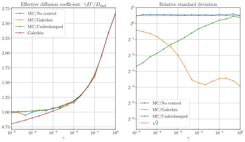
Figure 1: Effective diffusion coefficient and relative standard deviation $\frac{\sqrt{\mathbf{V}\bigl{[}v(T)\bigr{]}}}{D^{\gamma}}$ of the estimators considered at time $T=100/\gamma$. The data labeled “MC/No control” correspond to Monte Carlo simulations without a control variate, i.e. to the estimator $u(T)$ given in (2.1). The data labeled “MC/Galerkin” and “MC/Underdamped” correspond to the improved estimator (2.3), with $\psi$ obtained using the approaches of Sections 3.1 and 3.2, respectively. Finally, the curve labeled “Galerkin” is the approximate diffusion coefficient obtained by the Galerkin method alone, which is given by $\langle\widehat{\Psi}_{N},p\rangle$ in the notation of Section 3.1. The value $\sqrt{2}$ is the asymptotic relative standard deviation for the simple estimator $u(T)$, see Remark 2.7.

Figure 2 illustrates the evolution of the expectation and standard deviation of the estimators $u(t)$ given in (2.1) and $v(t)$ given in (2.5), empirically estimated from $J=5000$ realizations, with respect to the integration time $t$. It appears clearly that, for the value $\gamma=10^{-3}$ considered, the improved estimators $v(t)$ obtained using the approaches outlined in Sections 3.1 and 3.2 have a much smaller variance than $u(t)$ throughout the simulation.

Figure 2: Sample mean and sample standard deviation of the estimators $u(t)$ in (2.1) and $v(t)$ in (2.5), for the friction parameter $\gamma=10^{-3}$. The approximate solution to the Poisson equation used for constructing the control variate appearing in $v(t)$ here is that given in Section 3.2.

3.4 Extension to the generalized Langevin dynamics

The variance reduction approach described in Section 2, in particular with the control variate constructed from the limiting solution to the Poisson equation as $\gamma\to 0$, may be extended for calculating the mobility of simple generalized Langevin dynamics in one spatial dimension. The paradigmatic example dynamics we consider here is the following, which is studied in [37, 41]:

$$\left\{\begin{aligned} &\mathrm{d}q_{t}=p_{t}\,\mathrm{d}t,\\ &\mathrm{d}p_{t}=-V^{\prime}(q_{t})\,\mathrm{d}t+\frac{\sqrt{\gamma}}{\nu}\,z_{t}\,\mathrm{d}t,\\ &\mathrm{d}z_{t}=-\frac{\sqrt{\gamma}}{\nu}\,p_{t}\,\mathrm{d}t-\frac{1}{\nu^{2}}\,z_{t}\,\mathrm{d}t+\sqrt{\frac{2\beta^{-1}}{\nu^{2}}}\,\mathrm{d}w_{t},\end{aligned}\right.$$ (3.6)

where $z_{t}\in$. The unique invariant probability measure for this dynamics is given by

$$\mu_{\rm GLE}(\mathrm{d}q\,\mathrm{d}p\,\mathrm{d}z)\propto\exp\biggl{(}-\beta\left(H(q,p)+\frac{z^{2}}{2}\right)\biggr{)}\,\mathrm{d}q\,\mathrm{d}p\,\mathrm{d}z.$$

As proved in [36], a functional central limit theorem applies also to the dynamics (3.6): the diffusively rescaled position process $(\varepsilon q_{t/\varepsilon^{2}})_{t\geqslant 0}$ converges in distribution, in the Banach space of continuous functions over bounded time intervals, to a Brownian motion with diffusion coefficient $D^{\gamma,\nu}$. As in the case of the underdamped Langevin dynamics, this diffusion coefficient can be calculated in terms of the solution of an appropriate Poisson equation: $D^{\gamma,\nu}=\left\langle\phi,p\right\rangle$, where $\left\langle\,\cdot\,,\,\cdot\,\right\rangle$ is the inner product of $L^{2}(\mu_{\rm GLE})$ and $\phi$ is the unique solution to the following Poisson equation posed in $L^{2}_{0}(\mu_{\rm GLE})$:

$$-\mathcal{L}_{\rm GLE}\phi=p,$$ (3.7)

where $\mathcal{L}_{\rm GLE}$ is the generator of (3.6). As for the underdamped Langevin dynamics, the (Markovian approximation of the) generalized Langevin dynamics is difficult to understand in the underdamped regime, and in particular there does not exist a rigorous result on the behavior of $D^{\gamma,\nu}$ in the limit as $\gamma\to 0$. Our goal in this section is to calculate accurately the mobility for the dynamics (3.6) in the underdamped regime using a control variate approach similar to that described in Section 2, and to assess in this manner the validity of the asymptotic scaling for $D^{\gamma,\nu}$ conjectured in [41] by means of formal asymptotics. An application of Itô’s formula gives

$$q_{T}-q_{0}=\int_{0}^{T}p_{t}\,\mathrm{d}t=\phi(q_{0},p_{0},z_{0})-\phi(q_{T},p_{T},z_{T})+\sqrt{\frac{2\beta^{-1}}{\nu^{2}}}\int_{0}^{T}\partial_{z}\phi(q_{t},p_{t},z_{t})\,\mathrm{d}w_{t},$$

where $\phi$ is now the solution to (3.7). This motivates the following estimator for the mobility:

$$v(T)=d[\psi]+\frac{1}{2T}\left(\left|q_{T}-q_{0}\right|^{2}-\left|\xi_{T}\right|^{2}\right),\qquad d[\psi]:=\frac{\beta^{-1}}{\nu^{2}}\int\left|\partial_{z}\psi\right|^{2}\,\mathrm{d}\mu_{\rm GLE},$$ (3.8a)

where

$$\xi_{T}=\psi(q_{0},p_{0},z_{0})-\psi(q_{T},p_{T},z_{T})+\sqrt{\frac{2\beta^{-1}}{\nu^{2}}}\int_{0}^{T}\partial_{z}\psi(q_{t},p_{t},z_{t})\,\mathrm{d}w_{t},$$ (3.8b)

and $\psi$ is an approximate solution to the Poisson equation (3.7). The initial condition $(q_{0},p_{0},z_{0})$ is distributed according the invariant measure of the process, i.e. $\mu_{\rm GLE}$.

In [41], we employed an asymptotic expansion of the form $\phi=\gamma^{-1}\phi_{0}+\gamma^{-1/2}\phi_{1}+\gamma^{0}\phi_{2}+\dotsb$ in order to study the underdamped limit and we derived expressions for $\phi_{0}$ and $\phi_{1}$ which enable to show formally that $D^{\gamma,\nu}$ behaves as $1/\gamma$ in the limit as $\gamma\to 0$, with a prefactor $D^{\rm und}_{\nu}$ that can be efficiently calculated and is different from $D^{\rm und}$. (Recall from Section 1 that the diffusion coefficient $D^{\rm und}$ is defined as $D^{\rm und}=\lim_{\gamma\to 0}\gamma D^{\gamma}$, where $D^{\gamma}$ is the effective diffusion coefficient of the one-dimensional Langevin dynamics (1.6).) Although the assumed asymptotic expansion is shown to be invalid in [41] because $\mathcal{L}_{\rm GLE}\phi_{1}\notin L^{2}\left(\mu\right)$, our numerical results in this section demonstrate that this expansion can still be leveraged for constructing an efficient control variate $\xi_{T}$ in (3.8b). Specifically, we obtain a considerable reduction in variance by choosing the approximation $\psi$ in (3.8b) as $\psi=\gamma^{-1}\phi_{0}+\gamma^{-1/2}\phi_{1}$. We refer to [41, Section 4.3.2] for the expressions of the asymptotic value $D^{\nu}_{\rm und}$ and of the functions $\phi_{0}$ and $\phi_{1}$.

For the numerical integration of (3.6), we employ a numerical scheme similar to that presented in Section 3.3 for the Langevin dynamics. The scheme we use may be abbreviated as BABO using the terminology of [29], although it is not explicitly studied in that paper. More precisely, compared to the scheme used in Section 3.3, the last update for $p$ is replaced by the following simultaneous update for $p$ and $z$, corresponding to the analytical integration of the Ornstein–Uhlenbeck part of the dynamics:

$$\begin{pmatrix}p^{n+1}\\ z^{n+1}\end{pmatrix}=\mathrm{e}^{\boldsymbol{\mathbf{M}}\Delta t}\begin{pmatrix}p^{n}\\ z^{n}\end{pmatrix}+\int_{n\Delta t}^{(n+1)\Delta t}\mathrm{e}^{\boldsymbol{\mathbf{M}}\bigl{(}(n+1)\Delta t-s\bigr{)}}\begin{pmatrix}0\\ \sqrt{\frac{2\beta^{-1}}{\nu^{2}}}\end{pmatrix}\,\mathrm{d}w_{s},\qquad\boldsymbol{\mathbf{M}}=\begin{pmatrix}0&\frac{\sqrt{\gamma}}{\nu}\\ -\frac{\sqrt{\gamma}}{\nu}&-\frac{1}{\nu^{2}}\end{pmatrix}.$$

The Itô integral in this equation, which we denote by $\boldsymbol{\mathbf{I}}_{n}$, is a bivariate Gaussian with mean 0 and a covariance matrix independent of $n$. The covariance matrix is calculated from Itô’s isometry only once, at the beginning of the simulation. Likewise, the matrix exponential $\mathrm{e}^{\boldsymbol{\mathbf{M}}\Delta t}$ is precalculated before simulating the GLE dynamics.

The Itô integral in (3.8b) is discretized by using the Euler–Maruyama method. Since the Brownian increment $w_{(n+1)\Delta t}-w_{n\Delta t}$ is correlated to the Itô integral $\boldsymbol{\mathbf{I}}_{n}$, a technique similar to that presented Section 3.3 is required in order to generate $(\boldsymbol{\mathbf{I}}_{n},w_{(n+1)\Delta t}-w_{n\Delta t})$ at each iteration.

Figure 3 illustrates the evolution of $\mathbf{E}\bigl{[}u(t)\bigr{]}$ and $\mathbf{E}\bigl{[}v(t)\bigr{]}$, given in (2.1) and (3.8a), with respect to time, for a value of $\nu=2$ that is sufficiently large to observe a different asymptotic behavior in the limit as $\gamma\to 0$ than that of standard Langevin dynamics. These expectations are estimated from simulations using the same parameters as in Table 2. The associated $[m-3s,m+3s]$ confidence intervals (corresponding to a confidence of approximately $99.7\%$ assuming Gaussianity) are also depicted, where $m$ and $s$ are the sample mean and sample standard deviation. It is evident from the figures that the control variate leads to considerable improvements in terms of variance. Drawing conclusions on the bias is a more delicate task, as the true value of $D^{\gamma,\nu}$ is unknown, but it is clear that the improved estimator (3.8a) has a smaller bias for small times. Furthermore, we observe that the effective diffusion coefficient for $\gamma=10^{-5}$ is in very good agreement with the asymptotic equivalent $D^{\rm und}_{\nu}/\gamma$, where $D^{\rm und}_{\nu}=\lim_{\gamma\to 0}\gamma D^{\gamma,\nu}$ is the limiting value conjectured in [41]. The dependence of the effective diffusion coefficient on $\gamma$, calculated using the control variate, is presented in Figure 4.

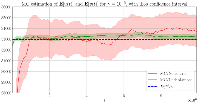
Figure 3: Expectations of the naive (2.1) and improved (3.8a) estimators for generalized Langevin dynamics and associated “$m\pm 3s$” confidence intervals, estimated from $J=5000$ realizations.

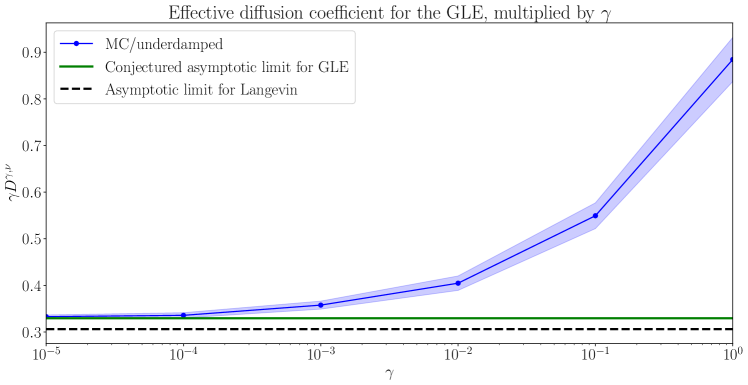
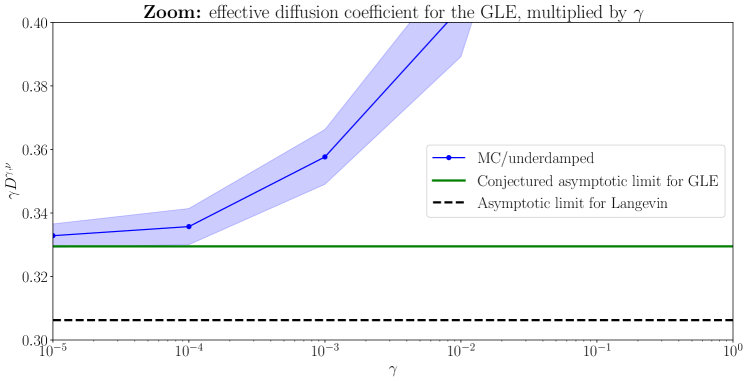
Figure 4: Expectation and “$m\pm 3s$” confidence intervals for $\gamma\mathbf{E}[v(T)]$ in the underdamped limit, for generalized Langevin dynamics with $\nu=2$. Since $T$ scales as $1/\gamma$ with a large prefactor, it is expected that $\mathbf{E}\bigl{[}v(T)\bigr{]}\approx D^{\gamma,\nu}$.

4 Application to Langevin dynamics in two dimensions

The approaches employed in Section 3 for constructing an approximate solution to the Poisson equation (1.7) do not generalize well to the multi-dimensional setting for non-separable potentials. On one hand, Galerkin methods for the Poisson equation suffer from the curse of dimensionality and, on the other hand, the behavior of the solution to the Poisson equation is not well understood in the underdamped limit. In this section, we discuss alternative approaches. We begin by showing that, under symmetry assumptions on the potential $V$, the diffusion tensor $\boldsymbol{\mathbf{D}}^{\gamma}$ is isotropic.

Lemma 4.1.

If $V$ satisfies the symmetry relation $V(q_{1},q_{2})=V(q_{2},q_{1})$, then $D^{\gamma}_{11}=D^{\gamma}_{22}$. In addition, if $V(q_{1},q_{2})=V(q_{1},-q_{2})$ or $V(q_{1},q_{2})=V(-q_{1},q_{2})$, then $D_{12}=0$.

Proof.

The first claim is obvious by symmetry. Here we prove only that $D^{\gamma}_{12}=0$ if the potential satisfies $V(q_{1},q_{2})=V(q_{1},-q_{2})$. To this end, let $\mathcal{R}$ be the operator on $L^{2}_{0}(\mu)$ defined by $\mathcal{R}f(q_{1},p_{1},q_{2},p_{2})=f(q_{1},p_{1},-q_{2},-p_{2})$. A simple calculation shows that $\mathcal{R}\mathcal{L}\mathcal{R}=\mathcal{L}$ and so, denoting by $\phi_{1}$ the solution to $-\mathcal{L}\phi_{1}=p_{1}$ posed on $L^{2}_{0}(\mu)$, we have $-\mathcal{R}\mathcal{L}\mathcal{R}\phi_{1}=p_{1}$. This implies $-\mathcal{L}\mathcal{R}\phi_{1}=p_{1}$ because $\mathcal{R}^{2}=\operatorname{id}$, so $\phi_{1}=\mathcal{R}\phi_{1}$ by uniqueness of the solution to the Poisson equation. It then follows that $D^{\gamma}_{12}=\left\langle\phi_{1},p_{2}\right\rangle=0$. ∎

We consider in this work a non-separable potential even simpler than (1.11):

$$V(q)=\mathcal{V}(q_{1})+\mathcal{V}(q_{2})+\delta\mathcal{W}(q_{1},q_{2}):=-\frac{\cos(q_{1})+\cos(q_{2})}{2}-\delta\cos(q_{1})\cos(q_{2}).$$ (4.1)

This potential satisfies the symmetry assumption of Lemma 4.1, and so the corresponding diffusion tensor is isotropic. Therefore, in order to simplify the discussion, we focus on estimating $D^{\gamma}_{\boldsymbol{\mathbf{e}}}$ only for the unit vector $\boldsymbol{\mathbf{e}}=(1,0)^{\mathsf{T}}$. Accordingly, let $\phi_{\delta}(q,p)$ denote the solution to the Poisson equation $-\mathcal{L}^{\delta}\phi_{\delta}=p_{1}$, where the generator $\mathcal{L}^{\delta}$ of the dynamics now reads

$$\mathcal{L}^{\delta}=\mathcal{L}_{0}+\delta\mathcal{L}_{1}:=L_{1}+L_{2}-\delta\nabla\mathcal{W}\cdot\nabla_{\boldsymbol{\mathbf{p}}},$$ (4.2)

with $L_{i}=p_{i}\partial_{q_{i}}-\mathcal{V}^{\prime}(q_{i})\,\partial_{p_{i}}+\gamma\left(-p_{i}\partial_{p_{i}}+\beta^{-1}\partial^{2}_{p_{i}}\right)$ for $i\in\{1,2\}$. Notice that $\phi_{\delta}(\boldsymbol{\mathbf{q}},\boldsymbol{\mathbf{p}})=\phi_{\rm 1D}(q_{1},p_{1})$ when $\delta=0$, with $\phi_{\rm 1D}$ the solution to the one-dimensional Poisson equation $-L_{1}\phi_{\rm 1D}(q_{1},p_{1})=p_{1}$. In other words, it holds in this case that $\phi_{0}=\phi_{\rm 1D}\otimes 1$, where for two functions $f_{1}:\mathbf{T}\times\rightarrow$ and $f_{2}:\mathbf{T}\times\rightarrow$ the notation $f_{1}\otimes f_{2}$ denotes the function $(\boldsymbol{\mathbf{q}},\boldsymbol{\mathbf{p}})\mapsto f_{1}(q_{1},p_{1})\,f_{2}(q_{2},p_{2})$. For small $\delta$, it is natural to use $\phi_{0}$, or an approximation thereof, as the function $\psi_{\boldsymbol{\mathbf{e}}}$ in the definition of the control variate (2.3). Note that $d[\psi_{\boldsymbol{\mathbf{e}}}]$ in (2.3) is an average with respect to the invariant distribution of the non-separable dynamics, which we denote by $\mu_{\delta}$ to emphasize the dependence on $\delta$. Specifically, we have

$$d[\psi_{\boldsymbol{\mathbf{e}}}]=\int_{\mathbf{T}^{2}\times^{2}}\left|\nabla_{\boldsymbol{\mathbf{p}}}\psi_{\boldsymbol{\mathbf{e}}}\right|^{2}\,\mathrm{d}\mu_{\delta}.$$ (4.3)

The following result establishes that $\phi_{\delta}$ converges to $\phi_{0}$ in $L^{2}(\mu)$ in the limit as $\delta\to 0$.

Proposition 4.2.

Let $\phi_{\delta}$ and $\phi_{0}$ denote the solutions to the Poisson equation $-\mathcal{L}^{\delta}\phi_{\delta}=p_{1}$ and its separable counterpart $-\mathcal{L}_{0}\phi_{0}=p_{1}$, these equations being posed in $L^{2}_{0}(\mu_{\delta})$ and $L^{2}_{0}(\mu_{0})$, respectively. Then there exists $C>0$ independent of $\delta$ and $\gamma$ such that

$$\forall(\gamma,\delta)\in(0,\infty)\times[-1,1],\qquad$$

$$\qquad\|\phi_{\delta}-\phi_{0}\|_{L^{2}(\mu_{\delta})}\leqslant C\lvert\delta\rvert\left(\max\bigl{\{}\gamma,\gamma^{-1}\bigr{\}}\left\|\nabla_{\boldsymbol{\mathbf{p}}}\phi_{0}\right\|_{L^{2}(\mu_{\delta})}+\left\|\phi_{0}\right\|_{L^{2}(\mu_{\delta})}\right),$$ (4.4)

and

$$\forall(\gamma,\delta)\in(0,\infty)\times[-1,1],\qquad\|\nabla_{\boldsymbol{\mathbf{p}}}\phi_{\delta}-\nabla_{\boldsymbol{\mathbf{p}}}\phi_{0}\|_{L^{2}(\mu_{\delta})}\leqslant C\lvert\delta\rvert\max\bigl{\{}1,\gamma^{-1}\bigr{\}}\left\|\nabla_{\boldsymbol{\mathbf{p}}}\phi_{0}\right\|_{L^{2}(\mu_{\delta})}.$$ (4.5)

Before we present the proof of this result, a couple of remarks are in order.

Remark 4.1.

There exist constants $c_{1},c_{2}>0$ such that

$$\forall\delta\in[-1,1],\qquad c_{1}\left\|\,\cdot\,\right\|_{L^{2}(\mu_{\delta})}\leqslant\left\|\,\cdot\,\right\|_{L^{2}(\mu_{0})}\leqslant c_{2}\left\|\,\cdot\,\right\|_{L^{2}(\mu_{\delta})},$$

and so the inequalities (4.4) and (4.5) are valid also with $\left\|\,\cdot\,\right\|_{L^{2}(\mu_{\delta})}$ replaced by $\left\|\,\cdot\,\right\|_{L^{2}(\mu_{0})}$.

Remark 4.2.

Using the definition (4.3) and Proposition 4.2, we deduce that

$$\forall(\gamma,\delta)\in(0,1)\times[-1,1],\qquad\frac{\left\lvert\sqrt{d[\phi_{\delta}]}-\sqrt{d[\phi_{0}]}\right\rvert}{\sqrt{d[\phi_{0}]}}\leqslant C\lvert\delta\rvert\gamma^{-1}.$$

Consequently, since if $\left|\sqrt{x}-1\right|\leqslant\varepsilon$ for $x\geqslant 0$ then $\left|x-1\right|=\left|\sqrt{x}-1\right|\left|\sqrt{x}+1\right|\leqslant\varepsilon(2+\varepsilon)$,

$$\forall(\gamma,\delta)\in(0,1)\times[-1,1],\qquad\frac{\lvert d[\phi_{\delta}]-d[\phi_{0}]\rvert}{d[\phi_{0}]}\leqslant C\lvert\delta\rvert\gamma^{-1}(2+C\lvert\delta\rvert\gamma^{-1}).$$

In particular, for $\delta/\gamma$ fixed and sufficiently small, it holds that $\liminf_{\gamma\to 0}\gamma D^{\gamma}_{\boldsymbol{\mathbf{e}}}>0$; that is, the effective diffusion coefficient scales as $\gamma^{-1}$ in this case. (Of course, this does not say anything about the behavior of the diffusion coefficient for $\left|\delta\right|>0$ fixed and $\gamma\to 0$.)

Proof.

Let $\phi_{0}^{\delta}$ denote the $L^{2}(\mu_{\delta})$ orthogonal projection of $\phi_{0}$ onto $L^{2}_{0}(\mu_{\delta})$. We consider the decomposition (4.2) of the generator and note that

$$\mathcal{L}^{\delta}(\phi_{\delta}-\phi_{0}^{\delta})=\mathcal{L}^{\delta}(\phi_{\delta}-\phi_{0})=-\delta\,\mathcal{L}_{1}\phi_{0}=\delta\,\nabla\mathcal{W}\,\cdot\nabla_{\boldsymbol{\mathbf{p}}}\phi_{0}.$$ (4.6)

It follows from (4.6) that

$$\left\|\phi_{\delta}-\phi_{0}^{\delta}\right\|_{L^{2}(\mu_{\delta})} \leqslant\lvert\delta\rvert\left\|(\mathcal{L}^{\delta})^{-1}\right\|_{\mathcal{B}\left(L^{2}_{0}(\mu_{\delta})\right)}\left\|\nabla\mathcal{W}\,\cdot\nabla_{\boldsymbol{\mathbf{p}}}\phi_{0}\right\|_{L^{2}(\mu_{\delta})}.$$

From the results in [4, Section 3.1] which, as discussed in Section 2.2.1, were shown in various other works, it is clear that $\|(\mathcal{L}^{\delta})^{-1}\|_{\mathcal{B}\left(L^{2}_{0}(\mu_{\delta})\right)}$ is bounded from above by $K(\delta)\max\{\gamma,\gamma^{-1}\}$ for all $\gamma\in(0,\infty)$, with a constant $K(\delta)$ depending on $\delta$. A careful inspection of the result in [4] and its proof reveal that $K(\delta)$, which depends on $\delta$ through the Poincaré constant of $\mu_{\delta}$ among other things, is in fact such that $\sup\{K(\delta):-1\leqslant\delta\leqslant 1\}<\infty$. Therefore, using in addition that $\nabla\mathcal{W}$ is uniformly bounded, we obtain that

$$\forall(\gamma,\delta)\in(0,\infty)\times[-1,1],\qquad\left\|\phi_{\delta}-\phi_{0}^{\delta}\right\|_{L^{2}(\mu_{\delta})} \leqslant C\lvert\delta\rvert\max\{\gamma,\gamma^{-1}\}\left\|\nabla_{\boldsymbol{\mathbf{p}}}\phi_{0}\right\|_{L^{2}(\mu_{\delta})}.$$ (4.7)

Here and throughout this proof, $C$ denotes a constant independent of $\gamma$ and $\delta$, whose value can change from occurrence to occurrence. In order to show (4.4), it remains to bound $\|\phi_{0}^{\delta}-\phi_{0}\|$; the result then follows from the triangle inequality. To this end, note that $\mathrm{d}\mu_{\delta}/\mathrm{d}\mu_{0}=1+\delta f_{\delta}(q_{1},q_{2})$ for some appropriate smooth function $f_{\delta}$ that is $0$ if $\delta=0$ and is otherwise given explicitly by

$$f_{\delta}(q_{1},q_{2})=\frac{1}{\delta}\left(\frac{Z(0)}{Z(\delta)}\mathrm{e}^{-\beta\delta\mathcal{W}(q_{1},q_{2})}-1\right),\qquad Z(\delta)=\int_{\mathbf{T}\times\mathbf{T}}\mathrm{e}^{-\beta\bigl{(}\mathcal{V}(q_{1})+\mathcal{V}(q_{2})+\delta\mathcal{W}(q_{1},q_{2})\bigr{)}}\,\mathrm{d}q_{1}\mathrm{d}q_{2}.$$

Denoting by $M$ the supremum of $\beta|\mathcal{W}|$ over $\mathbf{T}^{2}$, we have $\mathrm{e}^{-\lvert\delta\rvert M}\leqslant Z(\delta)/Z(0)\leqslant\mathrm{e}^{\lvert\delta\rvert M}$, which implies that $\lvert f_{\delta}(q_{1},q_{2})\rvert\leqslant\lvert\delta\rvert^{-1}(\mathrm{e}^{2\lvert\delta\rvert M}-1)\leqslant 2M\mathrm{e}^{2M}$ uniformly for $(\delta,q_{1},q_{2})\in[-1,1]\times\mathbf{T}\times\mathbf{T}$. Therefore, using that $\phi_{0}$ has average 0 with respect to $\mu_{0}$,

$$\|\phi_{0}^{\delta}-\phi_{0}\|_{L^{2}(\mu_{\delta})}=\left|\int_{\mathbf{T}^{2}\times^{2}}\phi_{0}\,\mathrm{d}\mu_{\delta}\right|=\left|\int_{\mathbf{T}^{2}\times^{2}}\phi_{0}\,\bigl{(}1+\delta f_{\delta}(q_{1},q_{2})\bigr{)}\mathrm{d}\mu_{0}\right|\leqslant C\lvert\delta\rvert\left\|\phi_{0}\right\|_{L^{2}(\mu_{0})}.$$

which leads to (4.4) in view of Remark 4.1.

We now show (4.5). Taking the $L^{2}(\mu_{\delta})$ inner product of both sides of (4.6) with $\phi_{\delta}-\phi_{0}^{\delta}$, noting that $\nabla_{\boldsymbol{\mathbf{p}}}\phi_{0}^{\delta}=\nabla_{\boldsymbol{\mathbf{p}}}\phi_{0}$ and using (4.7), we obtain, for all $(\gamma,\delta)\in(0,\infty)\times[-1,1]$,

$$\gamma\beta^{-1}\|\nabla_{\boldsymbol{\mathbf{p}}}\phi_{\delta}-\nabla_{\boldsymbol{\mathbf{p}}}\phi_{0}\|_{L^{2}(\mu_{\delta})}^{2} \leqslant\lvert\delta\rvert\|\nabla\mathcal{W}\cdot\nabla_{\boldsymbol{\mathbf{p}}}\phi_{0}\|_{L^{2}(\mu_{\delta})}\|\phi_{\delta}-\phi_{0}^{\delta}\|_{L^{2}(\mu_{\delta})}$$

$$\leqslant C\lvert\delta\rvert\|\nabla_{\boldsymbol{\mathbf{p}}}\phi_{0}\|_{L^{2}(\mu_{\delta})}\|\phi_{\delta}-\phi_{0}^{\delta}\|_{L^{2}(\mu_{\delta})}$$

$$\leqslant C\delta^{2}\max\{\gamma,\gamma^{-1}\}\|\nabla_{\boldsymbol{\mathbf{p}}}\phi_{0}\|_{L^{2}(\mu_{\delta})}^{2},$$

which gives the claimed result. ∎

A direct corollary of Proposition 4.2 is that, if the exact solution to the Poisson equation in one spatial dimension is employed for constructing the control variate, i.e. if $\psi_{\boldsymbol{\mathbf{e}}}=\phi_{0}$ in the control variate (2.3), then by Proposition 2.7 and (4.5) we have

$$\lim_{T\to\infty}\mathbf{V}\bigl{[}v(T)\bigr{]} \leqslant 4\gamma\beta^{-1}\left\|\nabla_{\boldsymbol{\mathbf{p}}}\phi_{\delta}-\nabla_{\boldsymbol{\mathbf{p}}}\phi_{0}\right\|_{L^{2}(\mu_{\delta})}^{2}(d[\phi_{\delta}]+d[\phi_{0}])$$

$$\leqslant 4C\delta^{2}\gamma^{-1}\beta^{-1}\left\|\nabla_{\boldsymbol{\mathbf{p}}}\phi_{0}\right\|^{2}(d[\phi_{\delta}]+d[\phi_{0}])$$

$$=4C\delta^{2}\gamma^{-2}d[\phi_{0}](d[\phi_{\delta}]+d[\phi_{0}]),$$

which shows that, in this case, the asymptotic relative standard deviation admits an upper bound scaling as $\lvert\delta\rvert/\gamma$ in the limit as $\lvert\delta\rvert/\gamma\to 0$, provided that $\delta\in[-1,1]$ and $\gamma\in(0,1)$.

Figure 5 depicts the behavior of the mobility with respect to $\gamma$ for various values of $\delta$. For the sake of clarity, only the data calculated without a control variate, i.e. with the simple estimator $u(T)$ given in (2.1), is depicted in this figure. The reason for this choice is that, as we shall see in the next figure, the estimator $u(T)$ has the smallest variance when $\gamma\ll 1$ and $\delta/\gamma\gg 1$. It appears clearly from the figure that the mobility behaves, over the range of values of $\gamma$ we consider, as $\gamma^{-\sigma}$ for $\sigma\in(0,1]$ in the underdamped regime, with an exponent $\sigma$ that decreases as $\delta>0$ increases (at least for sufficiently small values of $\delta$). As mentioned in the introduction, it is an open problem to identify classes of potentials for which a universal scaling of the diffusion coefficient with respect to the friction can be rigorously shown in the nonseperable case.

The variance of the estimators obtained using the control approach described above, where $\psi_{\boldsymbol{\mathbf{e}}}$ is constructed from an approximate solution to the Poisson equation in the one-dimensional setting, is presented in Figure 6. The control variates corresponding to the data in the left and right panels are constructed with the Galerkin approach of Section 3.1 and the underdamped approach of Section 3.2, respectively. We observe that unless $\delta=0$, in which case we recover the one-dimensional case, there seems to be, for every $\delta>0$ and for each of the two choices of $\psi_{\boldsymbol{\mathbf{e}}}$, a threshold value of $\gamma$ below which the control variate ceases to be useful. This is not unexpected, in view of Proposition 4.2. Although the control variates we consider are advantageous in certain regimes, further work is necessary in order to develop efficient estimators in the small $\gamma$, constant $\delta$ regime.

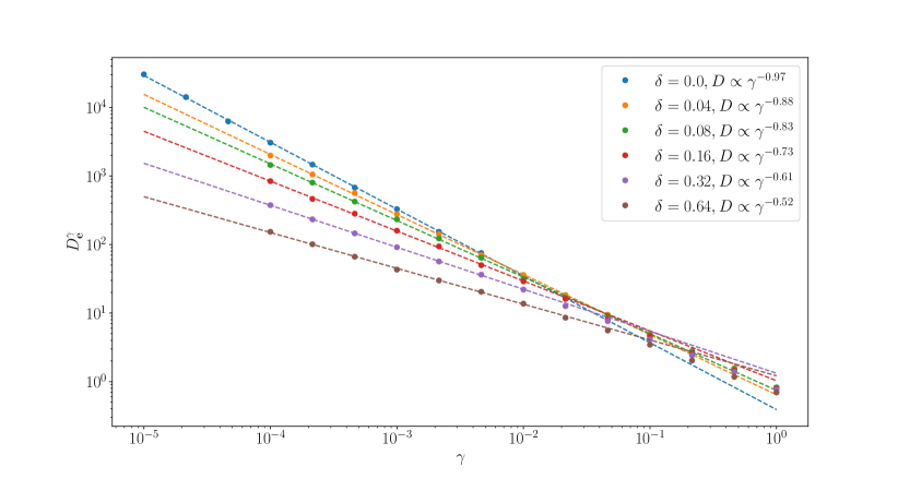
Figure 5: Effective diffusion coefficient as a function of $\gamma$, for various values of $\delta$. The straight dashed lines, which correspond to functions of the form $\gamma\mapsto C\gamma^{-\sigma}$ with powers $\sigma$ indicated in the legend, are obtained by linear interpolation (in the log-log plot) using only values of $\gamma$ less than or equal to $10^{-2}$.

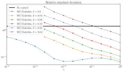
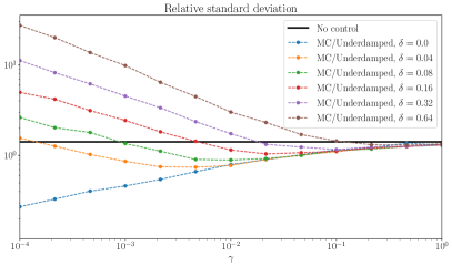
Figure 6: Relative standard deviation of the estimator $v(T)$ in (2.5) for two-dimensional Langevin dynamics, when the approximate solution to the Poisson equation is constructed by tensorization from the solution of the one-dimensional equation. The one-dimensional solution is approximated using either the Galerkin approach of Section 3.1 (left panel) or the underdamped approach of Section 3.2 (right panel).

5 Conclusions and perspectives for future work

In this work, we showed how techniques based on control variates can be employed for improving estimators of dynamical properties, here the mobility of Langevin dynamics based on Einstein’s formula. The control variate approach we propose requires the knowledge of an approximate solution to a Poisson equation involving the generator of the dynamics. We studied several practical approaches for constructing this approximate solution, and we obtain general bounds on the bias and variance of the proposed estimator in terms of the approximation error.

In the one-dimensional setting, we demonstrated the efficiency of control variates (i) obtained by a Fourier/Hermite spectral method for the Poisson equation, and (ii) based on an explicit expression for the limiting solution to the Poisson equation in the underdamped limit. For both Langevin and generalized Langevin dynamics, the latter approach leads to a significant variance reduction in the very small friction regime $\gamma\leqslant 10^{-3}$, in which fully deterministic Galerkin methods are inaccurate.

The numerical experiments we presented for the one-dimensional generalized Langevin dynamics also corroborate prior findings in [41], obtained through formal asymptotics, concerning the asymptotic behavior of the mobility in the small friction limit. More precisely, they indicate that the mobility scales as $1/\gamma$ as $\gamma\to 0$ when the parameter $\nu$ encoding memory is fixed, with a prefactor different from that corresponding to Langevin dynamics.

The two-dimensional setting for Langevin dynamics is much more challenging because of the high dimensionality of the state space of the dynamics and the lack of theoretical results for the underdamped limit in the case of a non-separable potential. Nevertheless, the control variates developed for one-dimensional Langevin dynamics may still be applied with appropriate tensorization, and we show by means of numerical experiments that they lead to estimators with reduced variance provided that the parameter multiplying the non-separable part of the potential is small with respect to the friction $\gamma$.

We anticipate that, in the future, approaches based on physics-informed neural networks (PINN) [48, 47] will be useful for constructing more accurate solutions to the Poisson equation (1.7) in two spatial dimensions than is possible using a Galerkin method, providing scope for greater variance reduction for Monte Carlo estimators of the mobility. The body of literature on the use of neural networks in the context of high-dimensional PDEs has grown very rapidly in recent years, and there is increasing evidence that these approaches are able to overcome the curse of dimensionality in a variety of PDE applications [21, 35, 26, 18, 24, 10, 25, pmlr-v145-zhai22a].

Acknowledgements.

The work of GS and UV was partially funded by the European Research Council (ERC) under the European Union’s Horizon 2020 research and innovation programme (grant agreement No 810367), and by the Agence Nationale de la Recherche under grant ANR-21-CE40-0006 (SINEQ). The work of GAP was partially supported by JPMorgan Chase & Co under J.P. Morgan A.I. Research Awards in 2019 and 2021 and by the EPSRC, grant number EP/P031587/1. The work of UV was partially funded by the Fondation Sciences Mathématiques de Paris (FSMP), through a postdoctoral fellowship in the “mathematical interactions” programme.

Appendix A Proof of Proposition 2.3

The proof is based on several lemmata. Before presenting these, we introduce some notation and recall useful background material. For a measure $\pi$, we define the weighted Sobolev space $H^{i}(\pi)$ as the subspace of $L^{2}(\pi)$ of functions whose derivatives up to order $i$ are in $L^{2}(\pi)$. The associated norm is given by

$$\left\|u\right\|_{i}^{2}=\sum_{|\boldsymbol{\mathbf{\alpha}}|\leqslant i}\|\partial^{\boldsymbol{\mathbf{\alpha}}}f\|^{2},$$

where we use the standard multi-index notation. Throughout this section, $\left\|\,\cdot\,\right\|$ and $\left\langle\,\cdot\,,\,\cdot\,\right\rangle$ are the norm and inner product of $L^{2}(\pi)$. The probability measure $\pi$ implicit in this notation will be either obvious in the context or explicitly specified. We recall that $\pi$ is said to satisfy a Poincaré inequality with constant $R$ if

$$\forall f\in H^{1}(\pi)\cap L^{2}_{0}(\pi),\qquad\|f\|^{2}\leqslant\frac{1}{R}\left\|\nabla f\right\|^{2}.$$ (P_R)

It is well known that the Gaussian measure $\kappa$ in (1.3) satisfies (P_R) with a constant $R_{\kappa}=\beta$; see, for example, [14, Lemma 2.1] for a short proof. We will use the following standard result which follows, for example, from [32, Chapter 9].

Lemma A.1.

It holds that

$$D(\mathcal{L}_{\rm FD}):=\Bigl{\{}f\in L^{2}_{0}(\kappa):\mathcal{L}_{\rm FD}f\in L^{2}_{0}(\kappa)\Bigr{\}}=H^{2}(\kappa)\cap L^{2}_{0}(\kappa).$$

In addition, the unbounded operator $\mathcal{L}_{\rm FD}$ with domain $D(\mathcal{L}_{\rm FD})$ has a discrete spectrum and generates a contraction semigroup $(\mathrm{e}^{t\mathcal{L}_{\rm FD}})_{t\geqslant 0}$ on $L^{2}_{0}(\kappa)$, with $\lVert\mathrm{e}^{t\mathcal{L}_{\rm FD}}f\rVert\leqslant\mathrm{e}^{-t}\lVert f\rVert$ for all $f\in L^{2}_{0}(\kappa)$ and $t\geqslant 0$.

The eigenfunctions of $\mathcal{L}_{\rm FD}$ are given by rescaled Hermite polynomials, which form a complete orthonormal set of $L^{2}(\kappa)$. The eigenvalue associated with the constant polynomial is 0, and all the other eigenvalues are integer numbers less than or equal to $-1$. We denote the normalized eigenfunctions by $(\mathscr{H}_{\boldsymbol{\mathbf{\alpha}}})_{\boldsymbol{\mathbf{\alpha}}\in\mathbf{N}^{d}}$ and the corresponding eigenvalues by $(-\lambda_{\boldsymbol{\mathbf{\alpha}}})_{\boldsymbol{\mathbf{\alpha}}\in\mathbf{N}^{d}}$. Then

$$\forall f\in L^{2}_{0}(\kappa),\qquad\mathrm{e}^{t\mathcal{L}_{\rm FD}}f=\sum_{\left|\boldsymbol{\mathbf{\alpha}}\right|\geqslant 1}\mathrm{e}^{-\lambda_{\boldsymbol{\mathbf{\alpha}}}t}\left\langle f,\mathscr{H}_{\boldsymbol{\mathbf{\alpha}}}\right\rangle\mathscr{H}_{\boldsymbol{\mathbf{\alpha}}}.$$ (A.1)

This formula can be employed to show the following estimates.

Corollary A.2.

If $f\in L^{2}_{0}(\kappa)$, then $\mathrm{e}^{t\mathcal{L}_{\rm FD}}f\in H^{1}(\kappa)$ for $t>0$ and

$$\forall t>0,\qquad\left\|\nabla_{\boldsymbol{\mathbf{p}}}\mathrm{e}^{t\mathcal{L}_{\rm FD}}f\right\|_{L^{2}(\kappa)}\leqslant\frac{C}{\sqrt{t}}\left\|f\right\|_{L^{2}(\kappa)}.$$ (A.2a)

On the other hand, if $$f\in H^{1}(\kappa)$$, then

$$\forall t\geqslant 0,\qquad\left\|\nabla_{\boldsymbol{\mathbf{p}}}\mathrm{e}^{t\mathcal{L}_{\rm FD}}f\right\|_{L^{2}(\kappa)}\leqslant\mathrm{e}^{-t}\left\|\nabla_{\boldsymbol{\mathbf{p}}}f\right\|_{L^{2}(\kappa)}.$$ (A.2b)

Proof.

Assume first that $f\in D(\mathcal{L}_{\rm FD})$. Then $\mathrm{e}^{t\mathcal{L}_{\rm FD}}f\in D(\mathcal{L}_{\rm FD})$ for all $t>0$ by the general properties of operator semigroups [44] and, using (A.1), we obtain

$$\left\|\nabla_{\boldsymbol{\mathbf{p}}}\mathrm{e}^{t\mathcal{L}_{\rm FD}}f\right\|_{L^{2}(\kappa)}^{2}=\beta\left\langle\mathcal{L}_{\rm FD}\mathrm{e}^{t\mathcal{L}_{\rm FD}}f,\mathrm{e}^{t\mathcal{L}_{\rm FD}}f\right\rangle=\sum_{\left|\boldsymbol{\mathbf{\alpha}}\right|\geqslant 1}\beta\lambda_{\boldsymbol{\mathbf{\alpha}}}\mathrm{e}^{-2\lambda_{\boldsymbol{\mathbf{\alpha}}}t}\lvert\left\langle f,\mathscr{H}_{\boldsymbol{\mathbf{\alpha}}}\right\rangle\rvert^{2}.$$ (A.3)

The first claim follows from the inequality $\lambda\mathrm{e}^{-2\lambda t}\leqslant\frac{\mathrm{e}^{-1}}{2t},$ which is valid for all $\lambda\in$. The second claim follows from the fact that $\mathrm{e}^{-2\lambda_{\boldsymbol{\mathbf{\alpha}}}t}\leqslant\mathrm{e}^{-2t}$ for all $|\boldsymbol{\mathbf{\alpha}}|\geqslant 1$.

Consider now the case where $f\in L^{2}(\kappa)$ does not necessarily belong to $D(\mathcal{L}_{\rm FD})$ and let

$$f_{n}=\sum_{0\leqslant\left|\boldsymbol{\mathbf{\alpha}}\right|\leqslant n}\left\langle f,\mathscr{H}_{\boldsymbol{\mathbf{\alpha}}}\right\rangle\mathscr{H}_{\boldsymbol{\mathbf{\alpha}}}\in D(\mathcal{L}_{\rm FD})$$

For fixed $t>0$, the sequence $(\mathrm{e}^{t\mathcal{L}_{\rm FD}}f_{n})_{n\in\mathbf{N}}$ is a Cauchy sequence in $H^{1}(\kappa)$ by (A.2a), and so it converges to a limit in $H^{1}(\kappa)$ which necessarily coincides with the $L^{2}(\kappa)$ limit $\mathrm{e}^{t\mathcal{L}_{\rm FD}}f$. We conclude by applying (A.2a) and (A.2b) to $f_{n}$ and taking the limit $n\to\infty$. ∎

Let us now introduce additional notation. We define $\nabla_{\boldsymbol{\mathbf{q}}}^{*}=\beta\nabla V(\boldsymbol{\mathbf{q}})-\nabla_{\boldsymbol{\mathbf{q}}}$ and $\nabla_{\boldsymbol{\mathbf{p}}}^{*}=\beta\boldsymbol{\mathbf{p}}-\nabla_{\boldsymbol{\mathbf{p}}}$, and note that these operators are formally the $L^{2}(\mu)$ adjoints of $\nabla_{\boldsymbol{\mathbf{q}}}$ and $\nabla_{\boldsymbol{\mathbf{p}}}$. Similarly, in one dimension we write $\partial_{q}^{*}=\beta V^{\prime}(q)-\partial_{q}$ and $\partial_{p}^{*}=\beta p-\partial_{p}$.

The next lemma provides an intermediate result for proving Proposition 2.3, and concerns Langevin dynamics over the state space $\mathbf{T}^{d}\times^{d}$. This result is sharper than what would be obtained from a simple application of (2.12), but not yet sufficient for obtaining optimal estimates for the bias of estimator (2.1). To lighten notations, we confine ourselves from now on to the one-dimensional setting in the proofs, but these carry over mutatis mutandis to the multi-dimensional case.

Lemma A.3.

Assume that $f\in L^{2}(\mu)$ is a smooth function such that $\nabla_{\boldsymbol{\mathbf{q}}}f\in L^{2}(\mu)$ and

$$\forall\boldsymbol{\mathbf{q}}\in\mathbf{T}^{d},\qquad\Pi_{\boldsymbol{\mathbf{p}}}f(\boldsymbol{\mathbf{q}})=\int_{{}^{d}}f(\boldsymbol{\mathbf{q}},\boldsymbol{\mathbf{p}})\,\kappa(\mathrm{d}\boldsymbol{\mathbf{p}})=0.$$ (A.4)

Then there exist constants $C>0$ and $\lambda>0$ independent of $\gamma$ and $f$ such that

$$\forall\gamma\geqslant 1,\qquad\forall t\geqslant 0,\qquad\|\mathrm{e}^{t\mathcal{L}}f\|\leqslant C\bigl{(}\left\|f\right\|+\left\|\nabla_{\boldsymbol{\mathbf{q}}}f\right\|\bigr{)}\left(\mathrm{e}^{-\gamma t}+\gamma^{-1}\mathrm{e}^{-\frac{\lambda t}{\gamma}}\right).$$ (A.5)

The key feature of (A.5) is that, when $\gamma\gg 1$, the prefactor $\gamma^{-1}$ multiplying the slow exponential $\mathrm{e}^{-\frac{\lambda t}{\gamma}}$ is small, showing that $\mathrm{e}^{t\mathcal{L}}f$ is small after a time of order $\mathcal{O}(\gamma^{-1})$.

Proof.

We prove the result for functions $f(q,p)$ of the form

$$f(q,p)=\mathrm{e}^{\frac{\beta}{2}H(q,p)}\sum_{i=0}^{N}\sum_{j=1}^{N}c_{ij}\,g_{i}(q)h_{j}(p),$$ (A.6)

where $g_{i}$ and $h_{j}$ are the basis functions defined in (3.3) and (3.4). The space of functions of this form is dense in $\bigl{\{}u\in(\operatorname{id}-\Pi_{p})L^{2}(\mu):\partial_{q}u\in L^{2}(\mu)\bigr{\}}$ endowed with the norm $\left\|u\right\|_{1,q}:=\left\|u\right\|+\left\|\partial_{q}u\right\|$, so the general result follows by density.

We expect that $\mathrm{e}^{t\mathcal{L}}f\approx\mathrm{e}^{t\gamma\mathcal{L}_{\rm FD}}f$ in an appropriate sense for $\gamma\gg 1$. Therefore, let us introduce $v(t)=\mathrm{e}^{t\mathcal{L}}f(q,p)-\mathrm{e}^{t\gamma\mathcal{L}_{\rm FD}}f(q,p)$ and show that $v(t)$ is small. In the expression $\mathrm{e}^{t\gamma\mathcal{L}_{\rm FD}}f(q,p)$, the variable $q$ should be viewed as a parameter. The function $v$ satisfies the initial value problem

$$\partial_{t}v=\mathcal{L}v+\mathcal{L}_{\rm Ham}\bigl{(}\mathrm{e}^{t\gamma\mathcal{L}_{\rm FD}}f\bigr{)},\qquad v(0)=0.$$

By Duhamel’s formula,

$$v(t)=\int_{0}^{t}\mathrm{e}^{(t-s)\mathcal{L}}\Bigl{(}\mathcal{L}_{\rm Ham}\bigl{(}\mathrm{e}^{s\gamma\mathcal{L}_{\rm FD}}f\bigr{)}\Bigr{)}\,\mathrm{d}s,$$

and therefore

$$\mathrm{e}^{t\mathcal{L}}f=\mathrm{e}^{t\gamma\mathcal{L}_{\rm FD}}f+\int_{0}^{t}\mathrm{e}^{(t-s)\mathcal{L}}\Bigl{(}\mathcal{L}_{\rm Ham}\bigl{(}\mathrm{e}^{s\gamma\mathcal{L}_{\rm FD}}f\bigr{)}\Bigr{)}\,\mathrm{d}s.$$ (A.7)

The first term is bounded as

$$\left\|\mathrm{e}^{t\gamma\mathcal{L}_{\rm FD}}f\right\|^{2} =\int_{\mathbf{T}}\int\left|\mathrm{e}^{t\gamma\mathcal{L}_{\rm FD}}f(q,p)\right|^{2}\kappa(\mathrm{d}p)\,\nu(\mathrm{d}q)=\int_{\mathbf{T}}\left\|\mathrm{e}^{t\gamma\mathcal{L}_{\rm FD}}f(q,\,\cdot\,)\right\|_{L^{2}(\kappa)}^{2}\,\nu(\mathrm{d}q)$$

$$\leqslant\int_{\mathbf{T}}\mathrm{e}^{-2\gamma t}\left\|f(q,\,\cdot\,)\right\|_{L^{2}(\kappa)}^{2}\,\nu(\mathrm{d}q)=\mathrm{e}^{-2\gamma t}\left\|f\right\|^{2},$$ (A.8)

where we employed Lemma A.1 in the second line. We now bound the second term on the right-hand side of (A.7). The commutator relation $[\partial_{p},\partial_{p}^{*}]=\beta$ implies that

$$\forall\varphi\in L^{2}(\kappa),\qquad\left\|\partial_{p}^{*}\varphi\right\|_{L^{2}(\kappa)}^{2}=\left\|\partial_{p}\varphi\right\|_{L^{2}(\kappa)}^{2}+\beta\left\|\varphi\right\|_{L^{2}(\kappa)}^{2}.$$

Using this equation together with the definition of $\partial_{q}^{*}$, we have

$$\left\|\partial_{q}\partial_{p}^{*}\mathrm{e}^{t\gamma\mathcal{L}_{\rm FD}}f\right\| \leqslant\left\|\partial_{q}\partial_{p}\mathrm{e}^{t\gamma\mathcal{L}_{\rm FD}}f\right\|+\sqrt{\beta}\left\|\partial_{q}\mathrm{e}^{t\gamma\mathcal{L}_{\rm FD}}f\right\|,$$

$$\left\|\partial_{q}^{*}\partial_{p}\mathrm{e}^{t\gamma\mathcal{L}_{\rm FD}}f\right\| \leqslant\left\|\partial_{q}\partial_{p}\mathrm{e}^{t\gamma\mathcal{L}_{\rm FD}}f\right\|+\beta\left\|V^{\prime}\right\|_{\infty}\left\|\partial_{p}\mathrm{e}^{t\gamma\mathcal{L}_{\rm FD}}f\right\|.$$

From these equations, we deduce

$$\left\|\mathcal{L}_{\rm Ham}\mathrm{e}^{t\gamma\mathcal{L}_{\rm FD}}f\right\| =\beta^{-1}\lVert(\partial_{q}\partial_{p}^{*}-\partial_{q}^{*}\partial_{p})\mathrm{e}^{t\gamma\mathcal{L}_{\rm FD}}f\rVert$$

$$\leqslant 2\beta^{-1}\left\|\partial_{q}\partial_{p}\mathrm{e}^{t\gamma\mathcal{L}_{\rm FD}}f\right\|+\beta^{-1/2}\left\|\partial_{q}\mathrm{e}^{t\gamma\mathcal{L}_{\rm FD}}f\right\|+\|V^{\prime}\|_{\infty}\left\|\partial_{p}\mathrm{e}^{t\gamma\mathcal{L}_{\rm FD}}f\right\|.$$ (A.9)

Since $f$ is assumed to be a finite linear combination of the form (A.6), we can freely change the order of the operators $\partial_{q}$ and $\mathrm{e}^{t\gamma\mathcal{L}_{\rm FD}}$; in particular, the function $\mathrm{e}^{t\gamma\mathcal{L}_{\rm FD}}f$ is differentiable in $q$. Letting $t_{*}=\min\{\gamma^{-1},t\}$, we have

$$\left\|\partial_{q}\partial_{p}\mathrm{e}^{t\gamma\mathcal{L}_{\rm FD}}f\right\| =\left\|\partial_{p}\mathrm{e}^{t\gamma\mathcal{L}_{\rm FD}}\partial_{q}f\right\|=\left\|\partial_{p}\mathrm{e}^{(t-t_{*})\gamma\mathcal{L}_{\rm FD}}(\mathrm{e}^{t_{*}\gamma\mathcal{L}_{\rm FD}}\partial_{q}f)\right\|$$

$$\leqslant\mathrm{e}^{-\gamma(t-t_{*})}\left\|\partial_{p}\mathrm{e}^{t_{*}\gamma\mathcal{L}_{\rm FD}}\partial_{q}f\right\|\leqslant C\frac{\mathrm{e}^{-\gamma(t-t_{*})}}{\sqrt{\gamma t_{*}}}\left\|\partial_{q}f\right\|,$$

where we applied (A.2b) in the first inequality, then (A.2a) in the second inequality. Bounding the other terms in (A.9) using the same method and observing that $\mathrm{e}^{\gamma t_{*}}\leqslant\mathrm{e}$, we obtain

$$\left\|\mathcal{L}_{\rm Ham}\mathrm{e}^{t\gamma\mathcal{L}_{\rm FD}}f\right\| \leqslant C\frac{\mathrm{e}^{-\gamma t}}{\sqrt{\min\{1,\gamma t\}}}\bigl{(}\left\|f\right\|+\left\|\partial_{q}f\right\|\bigr{)}.$$ (A.10)

Going back to (A.7) and using (2.12), we have, for $\gamma\geqslant 1$,

$$\|\mathrm{e}^{t\mathcal{L}}f\| \leqslant\mathrm{e}^{-\gamma t}\left\|f\right\|+C\bigl{(}\left\|f\right\|+\left\|\partial_{q}f\right\|\bigr{)}\int_{0}^{t}\mathrm{e}^{-\frac{\ell}{\gamma}(t-s)}\,\left(\frac{\mathrm{e}^{-\gamma s}}{\sqrt{\min\{1,\gamma s\}}}\right)\,\mathrm{d}s.$$ (A.11)

It is clear that (A.5) holds for all $t\in[0,\gamma^{-1}]$, provided that the prefactor on the right-hand side of that equation is sufficiently large. To obtain (A.5) for times larger than $1/\gamma$, we bound the integral on the right-hand side of (A.11) by decomposing the interval $[0,t]$ as $[0,\frac{1}{\gamma}]\cup[\frac{1}{\gamma},t]$:

$$\int_{0}^{t}\mathrm{e}^{-\frac{\ell}{\gamma}(t-s)}\,\left(\frac{\mathrm{e}^{-\gamma s}}{\sqrt{\min\{1,\gamma s\}}}\right)\,\mathrm{d}s\leqslant\mathrm{e}^{-\frac{\ell}{\gamma}\left(t-\frac{1}{\gamma}\right)}\int_{0}^{\frac{1}{\gamma}}\frac{1}{\sqrt{\gamma s\,}}\,\mathrm{d}s+\int_{\frac{1}{\gamma}}^{t}\mathrm{e}^{-\frac{\ell}{\gamma}(t-s)-\gamma s}\mathrm{d}s$$

$$\qquad\leqslant\frac{2}{\gamma}\mathrm{e}^{-\frac{\ell}{\gamma}\left(t-\frac{1}{\gamma}\right)}+\int_{0}^{t}\mathrm{e}^{-\frac{\lambda}{\gamma}(t-s)-\gamma s}\mathrm{d}s$$

$$\qquad\leqslant\frac{2}{\gamma}\mathrm{e}^{-\frac{\ell}{\gamma}\left(t-\frac{1}{\gamma}\right)}+\int_{0}^{\infty}\mathrm{e}^{-\frac{\lambda}{\gamma}(t-s)-\gamma s}\mathrm{d}s\leqslant C\gamma^{-1}\mathrm{e}^{-\frac{\lambda t}{\gamma}},$$ (A.12)

where $\lambda=\min\{\frac{1}{2},\ell\}$. Defining $\lambda$ in this manner ensures that the integral on the last line is bounded for all $\gamma\in[1,\infty)$. The conclusion then follows from (A.11) and (A.12). ∎

We are now ready to prove Proposition 2.3.

Proof of Proposition 2.3.

We again show the result for functions $f$ and $h$ of the form (A.6), noting that the general result follows by density of functions of this type. Recall that, by assumption, both $f$ and $h$ are in $\Pi_{p}^{\perp}L^{2}(\mu)$, and their derivatives with respect to $q$ are in $L^{2}(\mu)$. From (A.7), we obtain

$$\left\langle\mathrm{e}^{t\mathcal{L}}f,h\right\rangle =\left\langle\mathrm{e}^{t\gamma\mathcal{L}_{\rm FD}}f,h\right\rangle+\int_{0}^{t}\left\langle\mathrm{e}^{(t-s)\mathcal{L}}\Bigl{(}\mathcal{L}_{\rm Ham}\bigl{(}\mathrm{e}^{s\gamma\mathcal{L}_{\rm FD}}f\bigr{)}\Bigr{)},h\right\rangle\,\mathrm{d}s$$

$$=\left\langle\mathrm{e}^{t\gamma\mathcal{L}_{\rm FD}}f,h\right\rangle+\int_{0}^{t}\left\langle\mathcal{L}_{\rm Ham}\bigl{(}\mathrm{e}^{s\gamma\mathcal{L}_{\rm FD}}f\bigr{)},\mathrm{e}^{(t-s)\mathcal{L}^{*}}h\right\rangle\,\mathrm{d}s.$$ (A.13)

The first term is bounded as in (A.8). In order to bound the second term, we denote the $L^{2}(\mu)$ adjoint of the generator $\mathcal{L}$ by  $\mathcal{L}^{*}=-\mathcal{L}_{\rm Ham}+\gamma\mathcal{L}_{\rm FD}$, and employ the fact that Lemma A.3 is valid also with $\mathcal{L}^{*}$ substituted for $\mathcal{L}$, and so

$$\forall\gamma\geqslant 1,\quad\forall t\geqslant 0,\qquad\left\|\mathrm{e}^{(t-s)\mathcal{L}^{*}}h\right\|\leqslant C\bigl{(}\left\|h\right\|+\left\|\partial_{q}h\right\|\bigr{)}\left(\mathrm{e}^{-\gamma(t-s)}+\gamma^{-1}\mathrm{e}^{-\frac{\lambda(t-s)}{\gamma}}\right).$$

Combined with (A.10), this inequality gives

$$\left|\left\langle\mathrm{e}^{t\mathcal{L}}f,h\right\rangle\right|\leqslant\left\|f\right\|\left\|h\right\|\mathrm{e}^{-\gamma t}$$

$$\qquad+C\bigl{(}\left\|f\right\|+\left\|\partial_{q}f\right\|\bigr{)}\bigl{(}\left\|h\right\|+\left\|\partial_{q}h\right\|\bigr{)}\int_{0}^{t}\left(\frac{\mathrm{e}^{-\gamma s}}{\sqrt{\min\{1,\gamma s\}}}\right)\left(\mathrm{e}^{-\gamma(t-s)}+\gamma^{-1}\mathrm{e}^{-\frac{\lambda(t-s)}{\gamma}}\right)\,\mathrm{d}s.$$

The first term in the integral is bounded as

$$\int_{0}^{t}\left(\frac{\mathrm{e}^{-\gamma s}}{\sqrt{\min\{1,\gamma s\}}}\right)\mathrm{e}^{-\gamma(t-s)}\,\mathrm{d}s=\mathrm{e}^{-\gamma t}\left(\int_{0}^{\gamma^{-1}}\frac{1}{\sqrt{\gamma s}}\,\mathrm{d}s+t-\gamma^{-1}\right)=\mathrm{e}^{-\gamma t}\left(t+\frac{1}{\gamma}\right).$$

For any $\alpha\in(0,1)$, the right-hand side of this equation may be bounded from above by $C_{\alpha}\mathrm{e}^{-\alpha\gamma t}$ . The second term in the integral can be bounded as in (A.12) in the proof of Lemma A.3, which concludes the proof of Proposition 2.3. ∎

Appendix B Proof of the bound (2.20)

In order to prove the bound, we write

$$\left\langle\mathrm{e}^{t\mathcal{L}}(\boldsymbol{\mathbf{e}}^{\mathsf{T}}\boldsymbol{\mathbf{p}}),\boldsymbol{\mathbf{e}}^{\mathsf{T}}\boldsymbol{\mathbf{p}})\right\rangle-\left\langle\mathrm{e}^{t\mathcal{L}}\mathcal{L}\psi_{\boldsymbol{\mathbf{e}}},\mathcal{L}\psi_{\boldsymbol{\mathbf{e}}}\right\rangle= \left\langle\mathrm{e}^{t\mathcal{L}}(\boldsymbol{\mathbf{e}}^{\mathsf{T}}\boldsymbol{\mathbf{p}}),\boldsymbol{\mathbf{e}}^{\mathsf{T}}\boldsymbol{\mathbf{p}}+(\operatorname{id}-\Pi_{\boldsymbol{\mathbf{p}}})\mathcal{L}\psi_{\boldsymbol{\mathbf{e}}}\right\rangle$$

$$-\left\langle\mathrm{e}^{t\mathcal{L}}\bigl{(}\boldsymbol{\mathbf{e}}^{\mathsf{T}}\boldsymbol{\mathbf{p}}+(\operatorname{id}-\Pi_{\boldsymbol{\mathbf{p}}})\mathcal{L}\psi_{\boldsymbol{\mathbf{e}}}\bigr{)},(\operatorname{id}-\Pi_{\boldsymbol{\mathbf{p}}})\mathcal{L}\psi_{\boldsymbol{\mathbf{e}}}\right\rangle$$

$$-\left\langle\mathrm{e}^{t\mathcal{L}}(\operatorname{id}-\Pi_{\boldsymbol{\mathbf{p}}})\mathcal{L}\psi_{\boldsymbol{\mathbf{e}}},\Pi_{\boldsymbol{\mathbf{p}}}\mathcal{L}\psi_{\boldsymbol{\mathbf{e}}}\right\rangle-\left\langle\mathrm{e}^{t\mathcal{L}}\Pi_{\boldsymbol{\mathbf{p}}}\mathcal{L}\psi_{\boldsymbol{\mathbf{e}}},\mathcal{L}\psi_{\boldsymbol{\mathbf{e}}}\right\rangle.$$

The last two terms are bounded using the general bound on the Langevin semigroup (2.12):

$$\max\left\{\left|\left\langle\mathrm{e}^{t\mathcal{L}}(\operatorname{id}-\Pi_{\boldsymbol{\mathbf{p}}})\mathcal{L}\psi_{\boldsymbol{\mathbf{e}}},\Pi_{\boldsymbol{\mathbf{p}}}\mathcal{L}\psi_{\boldsymbol{\mathbf{e}}}\right\rangle\right|,\left|\left\langle\mathrm{e}^{t\mathcal{L}}\Pi_{\boldsymbol{\mathbf{p}}}\mathcal{L}\psi_{\boldsymbol{\mathbf{e}}},\mathcal{L}\psi_{\boldsymbol{\mathbf{e}}}\right\rangle\right|\right\}$$

$$\qquad\qquad\qquad\qquad\leqslant L\exp\left(-\ell\min\{\gamma,\gamma^{-1}\}t\right)\left\|\Pi_{\boldsymbol{\mathbf{p}}}\mathcal{L}\psi_{\boldsymbol{\mathbf{e}}}\right\|\left\|\mathcal{L}\psi_{\boldsymbol{\mathbf{e}}}\right\|.$$

The first two terms are bounded using Proposition 2.3:

$$\left|\left\langle\mathrm{e}^{t\mathcal{L}}(\boldsymbol{\mathbf{e}}^{\mathsf{T}}\boldsymbol{\mathbf{p}}),\boldsymbol{\mathbf{e}}^{\mathsf{T}}\boldsymbol{\mathbf{p}}+(\operatorname{id}-\Pi_{\boldsymbol{\mathbf{p}}})\mathcal{L}\psi_{\boldsymbol{\mathbf{e}}}\right\rangle\right| \leqslant C\beta^{-1/2}\|\boldsymbol{\mathbf{e}}^{\mathsf{T}}\boldsymbol{\mathbf{p}}+\mathcal{L}\psi_{\boldsymbol{\mathbf{e}}}\|_{1,\boldsymbol{\mathbf{q}}}\,\zeta(t),$$

$$\left|\left\langle\mathrm{e}^{t\mathcal{L}}\bigl{(}\boldsymbol{\mathbf{e}}^{\mathsf{T}}\boldsymbol{\mathbf{p}}+(\operatorname{id}-\Pi_{\boldsymbol{\mathbf{p}}})\mathcal{L}\psi_{\boldsymbol{\mathbf{e}}}\bigr{)},(\operatorname{id}-\Pi_{\boldsymbol{\mathbf{p}}})\mathcal{L}\psi_{\boldsymbol{\mathbf{e}}}\right\rangle\right| \leqslant C\|\boldsymbol{\mathbf{e}}^{\mathsf{T}}\boldsymbol{\mathbf{p}}+\mathcal{L}\psi_{\boldsymbol{\mathbf{e}}}\|_{1,\boldsymbol{\mathbf{q}}}\,\|\mathcal{L}\psi_{\boldsymbol{\mathbf{e}}}\|_{1,\boldsymbol{\mathbf{q}}}\,\zeta(t),$$

where $\zeta(t)=\gamma^{-2}\mathrm{e}^{-a\gamma^{-1}t}+\mathrm{e}^{-a\gamma t}$. Here we employed the fact that, for any $f\in L^{2}\left(\mu\right)$ such that also $\nabla_{\boldsymbol{\mathbf{q}}}f\in L^{2}\left(\mu\right)$, it holds

$$\left\|\nabla_{\boldsymbol{\mathbf{q}}}(\operatorname{id}-\Pi_{\boldsymbol{\mathbf{p}}})f\right\|=\left\|(\operatorname{id}-\Pi_{\boldsymbol{\mathbf{p}}})\nabla_{\boldsymbol{\mathbf{q}}}f\right\|\leqslant\left\|\nabla_{\boldsymbol{\mathbf{q}}}f\right\|.$$

and so $\left\|(\operatorname{id}-\Pi_{\boldsymbol{\mathbf{p}}})f\right\|_{1,\boldsymbol{\mathbf{q}}}\leqslant\left\|f\right\|_{1,\boldsymbol{\mathbf{q}}}$. The bound (2.20) is then obtained by repeating the reasoning in the proof of Proposition 2.5.

Appendix C Proof of equation (2.29)

By definition of the variance, we have

$$\mathbf{V}\Bigl{[}\left\lvert X^{T}_{1}\right\rvert^{2}-\left\lvert X^{T}_{2}\right\rvert^{2}\Bigr{]}=\mathbf{E}\Bigl{[}\left\lvert X^{T}_{1}\right\rvert^{4}+\left\lvert X^{T}_{2}\right\rvert^{4}-2\left\lvert X^{T}_{1}X^{T}_{2}\right\rvert^{2}\Bigr{]}-\Bigl{(}\mathbf{E}\Bigl{[}\left\lvert X^{T}_{1}\right\rvert^{2}-\left\lvert X^{T}_{2}\right\rvert^{2}\Bigr{]}\Bigr{)}^{2},$$

and so it is sufficient to prove that, in the limit as $T\to\infty$ and for $i\in\{1,2\}$,

$$\mathbf{E}\left[\left\lvert X^{T}_{i}\right\rvert^{4}\right]\to\mathbf{E}\left[\left\lvert X^{\infty}_{i}\right\rvert^{4}\right],\quad\mathbf{E}\left[\left\lvert X^{T}_{i}\right\rvert^{2}\right]\to\mathbf{E}\left[\left\lvert X^{\infty}_{i}\right\rvert^{2}\right],\quad\mathbf{E}\left[\left\lvert X^{T}_{1}X^{T}_{2}\right\rvert^{2}\right]\to\mathbf{E}\left[\left\lvert X^{T}_{1}X^{T}_{2}\right\rvert^{2}\right].$$ (C.1)

By the continuous mapping theorem, it holds from the convergence in law of $X^{T}$ to $X^{\infty}$ that

$$\lvert X^{T}_{i}\rvert^{4}\xrightarrow[T\to\infty]{\rm Law}\left\lvert X^{\infty}_{i}\right\rvert^{4},\qquad\lvert X^{T}_{i}\rvert^{2}\xrightarrow[T\to\infty]{\rm Law}\left\lvert X^{\infty}_{i}\right\rvert^{2},\qquad\left\lvert X^{T}_{1}X^{T}_{2}\right\rvert^{2}\xrightarrow[T\to\infty]{\rm Law}\left\lvert X^{T}_{1}X^{T}_{2}\right\rvert^{2}.$$

In order to prove (C.1), it is therefore sufficient [6, Theorem 3.5] to show that the random variables $\lvert X^{T}_{i}\rvert^{4}$, $\lvert X^{T}_{i}\rvert^{2}$ and $\lvert X^{T}_{1}X^{T}_{2}\rvert^{2}$ are uniformly integrable over $T\in[1,\infty)$. We check this condition carefully for $\lvert X^{T}_{2}\rvert^{4}$, noting that the same reasoning can be applied to the other terms. A sufficient condition for uniform integrability is that there is $\varepsilon>0$ such that

$$\sup_{T\in[1,\infty)}\mathbf{E}\left[\left\lvert X^{T}_{2}\right\rvert^{4+\varepsilon}\right]<\infty.$$

By definition, it holds that

$$X^{T}_{2}=\frac{\psi_{\boldsymbol{\mathbf{e}}}(\boldsymbol{\mathbf{q}}_{0},\boldsymbol{\mathbf{p}}_{0})-\psi_{\boldsymbol{\mathbf{e}}}(\boldsymbol{\mathbf{q}}_{T},\boldsymbol{\mathbf{p}}_{T})}{\sqrt{2T}}+\sqrt{\frac{\gamma}{\beta T}}\int_{0}^{T}\nabla_{\boldsymbol{\mathbf{p}}}\psi_{\boldsymbol{\mathbf{e}}}(\boldsymbol{\mathbf{q}}_{t},\boldsymbol{\mathbf{p}}_{t})\cdot\mathrm{d}\boldsymbol{\mathbf{w}}_{t},$$

and so, using manipulations similar to those in the proof of Proposition 2.6, including a moment inequality for Itô integrals [33, Theorem 7.1] and the standing assumption of a stationary initial condition, we have, for $T\geqslant 0$,

$$\mathbf{E}\left[\lvert X^{T}_{2}\rvert^{4+\varepsilon}\right]\leqslant C\left(\left\|\psi_{\boldsymbol{\mathbf{e}}}\right\|_{L^{4+\varepsilon}(\mu)}^{4+\varepsilon}+\left\|\nabla_{\boldsymbol{\mathbf{p}}}\psi_{\boldsymbol{\mathbf{e}}}\right\|_{L^{4+\varepsilon}(\mu)}^{4+\varepsilon}\right)<\infty.$$

References

- [1] Michael P Allen and Dominic J Tildesley “Computer Simulation of Liquids” Oxford University Press, 2017
- [2] Stefano Baroni et al. “Heat Transport in Insulators from Ab Initio Green–Kubo Theory” In Handbook of Materials Modeling: Applications: Current and Emerging Materials Springer International Publishing, 2020, pp. 809–844 DOI: 10.1007/978-3-319-44680-6˙12
- [3] Alain Bensoussan, Jacques-Louis Lions and George Papanicolaou “Asymptotic analysis for periodic structures” 5, Studies in Mathematics and its Applications North-Holland Publishing Co., Amsterdam-New York, 1978, pp. xxiv+700
- [4] E. Bernard, M. Fathi, A. Levitt and G. Stoltz “Hypocoercivity with Schur complements” Accepted for publication in Ann. H. Lebesgue In arXiv preprint 2003.00726, 2020
- [5] R. N. Bhattacharya “On the functional central limit theorem and the law of the iterated logarithm for Markov processes” In Z. Wahrsch. Verw. Gebiete 60.2, 1982, pp. 185–201 DOI: 10.1007/BF00531822
- [6] Patrick Billingsley “Convergence of Probability Measures”, Wiley Series in Probability and Statistics: Probability and Statistics John Wiley & Sons, Inc., New York, 1999 DOI: 10.1002/9780470316962
- [7] Nawaf Bou-Rabee and Houman Owhadi “Long-run accuracy of variational integrators in the stochastic context” In SIAM J. Numer. Anal. 48.1, 2010, pp. 278–297 DOI: 10.1137/090758842
- [8] O. M. Braun and R. Ferrando “Role of long jumps in surface diffusion” In Phys. Rev. E 65, 2002, pp. 061107
- [9] L. Y. Chen, M. R. Baldan and S. C. Ying “Surface diffusion in the low-friction limit: Occurrence of long jumps” In Phys. Rev. B 54.12 APS, 1996, pp. 8856 DOI: 10.1103/PhysRevB.54.8856
- [10] Tim De Ryck and Siddhartha Mishra “Error analysis for physics informed neural networks (PINNs) approximating Kolmogorov PDEs” In arXiv preprint 2106.14473, 2021
- [11] J. Dolbeault, C. Mouhot and C. Schmeiser “Hypocoercivity for kinetic equations with linear relaxation terms” In C. R. Math. Acad. Sci. Paris 347.9-10, 2009, pp. 511–516 DOI: 10.1016/j.crma.2009.02.025
- [12] J. Dolbeault, C. Mouhot and C. Schmeiser “Hypocoercivity for linear kinetic equations conserving mass” In Trans. Amer. Math. Soc. 367.6, 2015, pp. 3807–3828 DOI: 10.1090/S0002-9947-2015-06012-7
- [13] Jean Dolbeault, Axel Klar, Clément Mouhot and Christian Schmeiser “Exponential rate of convergence to equilibrium for a model describing fiber lay-down processes” In Appl. Math. Res. Express. AMRX, 2013, pp. 165–175 DOI: 10.1093/amrx/abs015
- [14] Guillaume Dujardin, Frédéric Hérau and Pauline Lafitte “Coercivity, hypocoercivity, exponential time decay and simulations for discrete Fokker-Planck equations” In Numer. Math. 144.3, 2020, pp. 615–697 DOI: 10.1007/s00211-019-01094-y
- [15] Albert Einstein “Über die von der Molekularkinetischen Theorie der Wärme geforderte Bewegung von in ruhenden Flüssigkeiten suspendierten Teilchen” In Ann. Phys. 4, 1905, pp. 549–560 DOI: 10.1002/andp.19053220806
- [16] Loris Ercole, Aris Marcolongo and Stefano Baroni “Accurate thermal conductivities from optimally short molecular dynamics simulations” In Sci. Rep. 7.1 Nature Publishing Group, 2017, pp. 1–11
- [17] Peter W. Glynn and Roberto Szechtman “Some new perspectives on the method of control variates” In Monte Carlo and Quasi-Monte Carlo Methods, 2000 (Hong Kong) Springer, Berlin, 2002, pp. 27–49
- [18] Philipp Grohs, Arnulf Jentzen and Diyora Salimova “Deep neural network approximations for Monte Carlo algorithms” In arXiv preprint 1908.10828, 2019
- [19] Martin Grothaus and Patrik Stilgenbauer “Hilbert space hypocoercivity for the Langevin dynamics revisited” In Methods Funct. Anal. Topology 22.2, 2016, pp. 152–168
- [20] M. Hairer and G. A. Pavliotis “From ballistic to diffusive behavior in periodic potentials” In J. Stat. Phys. 131.1, 2008, pp. 175–202 DOI: 10.1007/s10955-008-9493-3
- [21] Jiequn Han, Arnulf Jentzen and Weinan E “Solving high-dimensional partial differential equations using deep learning” In Proc. Natl. Acad. Sci. USA 115.34, 2018, pp. 8505–8510 DOI: 10.1073/pnas.1718942115
- [22] Inge S. Helland “Central limit theorems for martingales with discrete or continuous time” In Scand. J. Statist. 9.2, 1982, pp. 79–94
- [23] F. Hérau “Hypocoercivity and exponential time decay for the linear inhomogeneous relaxation Boltzmann equation” In Asymptot. Anal. 46.3-4, 2006, pp. 349–359
- [24] Martin Hutzenthaler, Arnulf Jentzen, Thomas Kruse and Tuan Anh Nguyen “A proof that rectified deep neural networks overcome the curse of dimensionality in the numerical approximation of semilinear heat equations” In Partial Differ. Equ. Appl. 1.2, 2020, pp. Paper No. 10, 34 DOI: 10.1007/s42985-019-0006-9
- [25] Martin Hutzenthaler et al. “Overcoming the curse of dimensionality in the numerical approximation of semilinear parabolic partial differential equations” In Proc. A. 476.2244, 2020, pp. 20190630, 25 DOI: 10.1098/rspa.2019.0630
- [26] Arnulf Jentzen, Diyora Salimova and Timo Welti “A proof that deep artificial neural networks overcome the curse of dimensionality in the numerical approximation of Kolmogorov partial differential equations with constant diffusion and nonlinear drift coefficients” In Commun. Math. Sci. 19.5, 2021, pp. 1167–1205 DOI: 10.4310/CMS.2021.v19.n5.a1
- [27] Dirk P Kroese, Thomas Taimre and Zdravko I Botev “Handbook of Monte Carlo Methods” 706, Wiley Series in Probability and Statistics John Wiley & Sons, 2013
- [28] B. Leimkuhler, C. Matthews and G. Stoltz “The computation of averages from equilibrium and nonequilibrium Langevin molecular dynamics” In IMA J. Numer. Anal. 36.1, 2016, pp. 13–79 DOI: 10.1093/imanum/dru056
- [29] Benedict Leimkuhler and Matthias Sachs “Efficient numerical algorithms for the generalized Langevin equation” In SIAM J. Sci. Comput. 44.1, 2022, pp. A364–A388 DOI: 10.1137/20M138497X
- [30] T. Lelièvre and G. Stoltz “Partial differential equations and stochastic methods in molecular dynamics” In Acta Numer. 25, 2016, pp. 681–880 DOI: 10.1017/S0962492916000039
- [31] Tony Lelièvre, Mathias Rousset and Gabriel Stoltz “Free Energy Computations: A Mathematical Perspective” Imperial College Press, London, 2010 DOI: 10.1142/9781848162488
- [32] L. Lorenzi and M. Bertoldi “Analytical Methods for Markov Semigroups” 283, Pure and Applied Mathematics (Boca Raton) Chapman & Hall/CRC, Boca Raton, FL, 2007
- [33] X. Mao “Stochastic Differential Equations and Applications” Horwood Publishing Limited, Chichester, 2008 DOI: 10.1533/9780857099402
- [34] E. Nelson “Dynamical Theories of Brownian Motion” Princeton University Press, Princeton, N.J., 1967
- [35] Nikolas Nüsken and Lorenz Richter “Solving high-dimensional Hamilton-Jacobi-Bellman PDEs using neural networks: perspectives from the theory of controlled diffusions and measures on path space” In Partial Differ. Equ. Appl. 2.4, 2021, pp. Paper No. 48, 48 DOI: 10.1007/s42985-021-00102-x
- [36] M. Ottobre “Asymptotic Analysis for Markovian Models in Non-Equilibrium Statistical Mechanics”, 2012
- [37] M. Ottobre and G. A. Pavliotis “Asymptotic analysis for the generalized Langevin equation” In Nonlinearity 24.5, 2011, pp. 1629–1653 DOI: 10.1088/0951-7715/24/5/013
- [38] T. Papamarkou, A. Mira and M. Girolami “Zero variance differential geometric Markov chain Monte Carlo algorithms” In Bayesian Anal. 9.1, 2014, pp. 97–127 DOI: 10.1214/13-BA848
- [39] G. Papanicolaou and S. R. S. Varadhan “Ornstein-Uhlenbeck process in a random potential” In Comm. Pure Appl. Math. 38.6, 1985, pp. 819–834 DOI: 10.1002/cpa.3160380611
- [40] G. A. Pavliotis “Stochastic Processes and Applications” 60, Texts in Applied Mathematics Springer, New York, 2014
- [41] G. A. Pavliotis, G. Stoltz and U. Vaes “Scaling limits for the generalized Langevin equation” In J. Nonlinear Sci. 31.1, 2021, pp. Paper No. 8 DOI: 10.1007/s00332-020-09671-4
- [42] G. A. Pavliotis and A. M. Stuart “Multiscale Methods: Averaging and Homogenization” 53, Texts in Applied Mathematics Springer, New York, 2008
- [43] G. A. Pavliotis and A. Vogiannou “Diffusive transport in periodic potentials: underdamped dynamics” In Fluct. Noise Lett. 8.2, 2008, pp. L155–L173 DOI: 10.1142/S0219477508004453
- [44] A. Pazy “Semigroups of linear operators and applications to partial differential equations” 44, Applied Mathematical Sciences Springer-Verlag, New York, 1983 DOI: 10.1007/978-1-4612-5561-1
- [45] Petr Plechac, Gabriel Stoltz and Ting Wang “Martingale product estimators for sensitivity analysis in computational statistical physics” In arXiv preprint 2112.00126, 2021
- [46] C. Rackauckas and Q. Nie “Differentialequations.jl – A performant and feature-rich ecosystem for solving differential equations in Julia” In J. Open Res. Softw. 5.1 Ubiquity Press, 2017, pp. 15 DOI: 10.5334/jors.151
- [47] M. Raissi, P. Perdikaris and G. E. Karniadakis “Physics-informed neural networks: a deep learning framework for solving forward and inverse problems involving nonlinear partial differential equations” In J. Comput. Phys. 378, 2019, pp. 686–707 DOI: 10.1016/j.jcp.2018.10.045
- [48] Maziar Raissi and George Em Karniadakis “Hidden physics models: machine learning of nonlinear partial differential equations” In J. Comput. Phys. 357, 2018, pp. 125–141 DOI: 10.1016/j.jcp.2017.11.039
- [49] J. Roussel and G. Stoltz “Spectral methods for Langevin dynamics and associated error estimates” In ESAIM: Math. Model. Numer. Anal. 52.3 EDP Sciences, 2018, pp. 1051–1083 DOI: 10.1051/m2an/2017044
- [50] Julien Roussel “Theoretical and Numerical Analysis of Non-Reversible Dynamics in Computational Statistical Physics”, 2018
- [51] Mathias Rousset, Yushun Xu and Pierre-André Zitt “A weak overdamped limit theorem for Langevin processes” In ALEA Lat. Am. J. Probab. Math. Stat. 17.1, 2020, pp. 1–21 DOI: 10.30757/alea.v17-01
- [52] William Sutherland “A dynamical theory of diffusion for non-electrolytes and the molecular mass of albumin” In London, Edinburgh Dublin Philos. Mag. J. Sci. 9.54 Taylor & Francis, 1905, pp. 781–785 DOI: 10.1080/14786440509463331
- [53] Mark E. Tuckerman “Statistical Mechanics: Theory and Molecular Simulation”, Oxford Graduate Texts Oxford University Press, 2010
- [54] Loup Verlet “Computer “experiments” on classical fluids. I. Thermodynamical properties of Lennard-Jones molecules” In Phys. Rev. 159.1 APS, 1967, pp. 98
- [55] C. Villani “Hypocoercivity” In Mem. Amer. Math. Soc. 202.950, 2009
- [56] Marian Von Smoluchowski “Zur kinetischen Theorie der Brownschen Molekularbewegung und der Suspensionen” In Ann. Phys. 326.14 Wiley Online Library, 1906, pp. 756–780 DOI: 10.1002/andp.19063261405