The Story of $1/e$: ALOHA-based and Reinforcement-Learning-based Random Access for Delay-Constrained Communications

Abstract

Motivated by the proliferation of real-time applications in multimedia communication systems, tactile Internet, and cyber-physical systems, supporting delay-constrained traffic becomes critical for such systems. In delay-constrained traffic, each packet has a hard deadline; when it is not delivered before its deadline is up, it becomes useless and will be removed from the system. In this work, we focus on designing random access schemes for delay-constrained wireless communications. We first investigate three ALOHA-based schemes and prove that the system timely throughput of all three schemes under corresponding optimal transmission probabilities asymptotically converges to $1/e$, same as the well-known throughput limit for delay-unconstrained ALOHA systems. The fundamental reason why ALOHA-based schemes cannot achieve asymptotical system timely throughput beyond $1/e$ is that all active ALOHA stations access the channel with the same probability in any slot. To go beyond $1/e$, we propose a reinforcement-learning-based scheme for delay-constrained wireless communications, called RLRA-DC, under which different stations collaboratively attain different transmission probabilities by only interacting with the access point. Our numerical result shows that the system timely throughput of RLRA-DC can be as high as 0.8 for tens of stations and can still reach 0.6 even for thousands of stations, much larger than $1/e$.

I Introduction

Wireless communication is shifting its role from connecting people to network everything in multiple vertical domains, many of which have hard delay constraint. Typical examples include multimedia communication systems such as real-time streaming and video conferencing [2], tactile Internet [3, 4], networked control systems (NCSs) such as remote control of unmanned aerial vehicles (UAVs) [5, 6], and cyber-physical systems (CPSs) such as medical tele-operations, X-by-wire vehicles/avionics, factory automation, and robotic collaboration [7]. In such applications, each packet has a hard deadline: if it is not delivered before the deadline, it becomes useless and will be removed from the system. As an indispensable part of communication systems, how to design efficient random access schemes to support such delay-constrained applications is important but introduces new challenges [8, 9]. In this work, we will investigate both traditional ALOHA-based random access schemes and model learning-based random access schemes for delay-constrained wireless communications.

Since Abramson’s invention in 1970 [10], ALOHA-type protocols have been widely used for multiple users to access a shared communication channel due to its extreme simplicity and decentralized nature. One popular type is slotted ALOHA, where users are synchronized and can only transmit at the beginning of a slot [11]. It is well-known that the optimal asymptotic system throughput of slotted ALOHA system is $1/e=36.8\%$ [12]. In addition, there are many works to investigate the stability region of slotted ALOHA, i.e., to characterize the feasible input rates under which the system can be stabilized in the sense that the size of all queues will not diverge to infinity [13, 14, 15, 16, 17, 18]. There are also many types of extension for slotted ALOHA protocol, including multi-packet reception[19, 16], framed slotted ALOHA [20, 21, 22], coded slotted ALOHA [23], slotted ALOHA with successive interference cancellation (SIC) [24], etc. These works focus on delay-unconstrained case in the sense that any packet can be delivered in however much time.

There have been a few works on slotted ALOHA with delay-constrained traffic. Birk et al. in [25] proposed a scheme to increase the capacity by dividing packets into multiple sub-packets and transmitting redundant coded copies of the sub-packets. Stefanovic et al. in [26] studied delay-constrained frameless ALOHA in the finite-length case. Malak et al. in [27] investigated how to maximize the throughput of a random access system subject to given constraints on latency and outage. Borst and Zubeldia in [28] studied the scaling result of the average delay of slotted ALOHA systems in terms of the number of stations. Zhang et al. in [29] investigated the system throughput and the optimal retransmission probability with delay-constrained saturated traffic in the sense that each station always has a new packet arrival once its queue becomes empty (namely each station always has a packet to transmit). We should note that such a saturated traffic model is rather impractical. For example, in NCSs and CPSs, the control messages usually arrive periodically. Thus, in this paper we analyze the slotted ALOHA system with a non-saturated delay-constrained traffic model. It is called frame-synchronized traffic patten, which was widely investigated in the packet scheduling policy design in the delay-constrained wireless communication community [30, 2].

In addition to traditional ALOHA-based random access schemes, recently there are also a few works on learning-based access protocol. Deep reinforcement learning (DRL) has been introduced into the random access scheme design in [31] and [32]. In [31], Yu et al. proposed a scheme, called deep-reinforcement learning multiple access (DLMA), adopted feedforward neural networks (FNN) as the deep neural network. [32] applied DRL into CSMA and designed a new CSMA variant, called CS-DLMA. Both [31] and [32] assume a saturated delay-unconstrained traffic pattern. Wu et al. designed an R-learning-based random access scheme in a two-user delay-constrained heterogeneous wireless network in [33]. Their proposed scheme, called tiny state-space R-learning random access (TSRA), achieves higher timely throughput, lower computation complexity than DLMA. In addition, [34] proposed an online-learning-based access scheme, called Learn2MAC, to provide delay guarantee and low energy consumption.

In this paper, centering around the well-known throughput limit $1/e$, we will first study three different delay-constrained slotted ALOHA schemes and then propose a reinforcement-learning-based random access scheme. The three ALOHA-based schemes are $p$-constant slotted ALOHA where the retransmission probability is a constant all the time, $p$-dynamic slotted ALOHA where the retransmission probability changes according to the number of active stations at any slot, and framed slotted ALOHA where each station randomly selects a slot in a frame to probabilistically transmit its packet. Since slotted ALOHA is a popular wireless access scheme, investigating the fundamental performance of slotted ALOHA protocol to deliver delay-constrained traffic will add understandings and shed light on the design of practical wireless access protocols. We theoretically prove that the system timely throughput of all three ALOHA-based schemes converges to $1/e$ as the number of stations goes to infinity, as summarized in Table I. The fundamental reason why ALOHA-based schemes cannot achieve asymptotical system timely throughput beyond $1/e$ is that all active ALOHA stations access the channel with the same probability in any slot. Since the number of active stations tends to be infinite as the number of total stations goes to infinity, the system timely throughput also converges to $1/e$. In order to go beyond $1/e$, we propose a Reinforcement-Learning-based Random Access scheme for Delay-Constrained communications, called RLRA-DC, which can effectively reduce the competition level among active stations and improve the system timely throughput. RLRA-DC is designed based on R-learning [35, 36, 37], a less-popular variant of reinforcement learning different from the widely used Q-learning.

In particular, our contributions of this paper are as follows:

• We prove that the maximum system timely throughput converges to $1/e=36.8\%$ as the number of stations $N$ goes to infinity for any hard delay $D$ for all three ALOHA-based schemes. This delay-constrained asymptotic result is the same as the asymptotic maximum system throughput for delay-unconstrained slotted ALOHA system with saturated traffic [12, Chapter 5.3.2]. For $p$-constant slotted ALOHA, we prove that the optimal retransmission probability behaves asymptotically as $1/N$.

• In the finite regime of $N$, we propose an algorithm with time complexity $O(\min\{D,N\}\cdot D)$ to compute the system timely throughput for $p$-constant slotted ALOHA (resp. $p$-dynamic slotted ALOHA) for any number of stations $N$, and any hard delay $D$, and any retransmission probability $p$ (resp. any retransmission policy $\boldsymbol{p}$). For $p$-dynamic slotted ALOHA, we further derive the closed-form optimal dynamic retransmission policy.

• For framed slotted ALOHA with finite $N$, we derive the closed-form optimal retransmission probability and the closed-form maximum system timely throughput.

• To go beyond $1/e$, we introduce reinforcement learning to design a novel random access scheme, called RLRA-DC, which can effectively reduce competition among active stations. Under our proposed random access scheme, stations in the system cooperate with each other to intelligently reduce the competition level to improve the system timely throughput.

• We conduct extensive simulations to confirm the correctness of our theoretical analysis for three ALOHA-based schemes. We also show that the system timely throughput of thousands of stations when our proposed RLRA-DC scheme is deployed reaches 0.6, which is much higher than $1/e$ of the ALOHA-based systems.

TABLE I: Main results on three different delay-constrained slotted ALOHA schemes. Here $D$ is the hard delay of all packets, $N$ is the total number of stations, and $n(t)$ is the number of active stations at slot $t$.

Scheme of Slotted ALOHA	System Timely Throughput	Retransmission Probability	Feedback	$N$	$n(t)$
$p$-constant	$\lim\limits_{N\to\infty}R^{*}(D,N)=\frac{1}{e}$	$\lim\limits_{N\to\infty}N\cdot p^{*}(D,N)=1$	✓	✓	✗
$p$-dynamic	$\lim\limits_{N\to\infty}R_{\textsf{dynamic}}^{*}(D,N)=\frac{1}{e}$	$p_{\textsf{dynamic}}^{*}(t)=\frac{1}{n(t)}$	✓	✓	✓
Framed	$R_{\textsf{framed}}^{*}(D,N)=\left\{\begin{array}[]{ll}\frac{N}{D-1}\cdot\left(\frac{D-1}{D}\right)^{N},&\hbox{if $N\leq D$;}\\ \left(1-\frac{1}{N}\right)^{N-1},&\hbox{if $N>D$.}\end{array}\right.$ $\lim\limits_{N\to\infty}R_{\textsf{framed}}^{*}(D,N)=\frac{1}{e}$	$p_{\textsf{framed}}^{*}(D,N)=\min\left\{\frac{D}{N},1\right\}$	✗	✓	✗

The rest of the paper is organized as follows. We describe our system model in Section II. For $p$-constant slotted ALOHA, we propose a polynomial-time algorithm to compute the system timely throughput in Section III and analyze its asymptotic performance in Section IV. In Section V, we analyze $p$-dynamic slotted ALOHA and framed slotted ALOHA. In Section VI, we propose the reinforcement-learning-based random access scheme RLRA-DC. We use simulation to validate our theoretical analysis and also demonstrate the beyond-$1/e$ performance of RLRA-DC. Section VIII concludes this paper.

II System Model

We consider $N$ stations which share a common wireless channel and they need to send delay-constrained data packets to a common receiver via the shared wireless channel, as shown in Fig. 1. All packets have the same size and time is slotted where the slot duration is the time to transmit a packet from a station to the receiver and receive the acknowledge from the receiver (or observe the channel output) about whether the packet has been successfully delivered or not. Such acknowledge model is common in the literature for slotted ALOHA [15, 19]. A station can only send a packet at the beginning of a slot. If only one station transmits, the packet will be delivered successfully. Otherwise, if two or more stations transmit in the same slot, a collision happens and all packets will be lost.

We assume that each packet has a hard delay $D\geq 1$. Once arriving at a station (say at slot $t$), a packet will expire and be removed from the system if it cannot be delivered in $D$ slots (i.e., before slot $t+D$). In the rest of this paper, we call $D$ the hard delay to refer to a time span, while we call $t+D$ the hard deadline to refer to a time instance. Such feature is fundamentally different from the delay-unconstrained scenario. In the delay-constrained scenario, the (arrival) traffic patten greatly influences the system performance. As an initial study, in this paper, we assume a frame-synchronized traffic pattern. It can find applications in NCSs and CPSs where the system generates the control packets/messsages periodically [38], and it was widely investigated in the packet scheduling policy design in the delay-constrained wireless communication community [30, 2]. In the frame-synchronized traffic pattern, starting from slot 1, all stations have a packet arrival every $D$ slots (which is also the hard delay of all packets). Staring from slot 1, every consecutive $D$ slots is called a frame. The first frame is from slot 1 to slot $D$; the second frame is from slot $D+1$ to slot $2D$; and so on. Every station has a packet arrival at the beginning of a frame and the packet expires at the end of the frame. Fig. 1 shows an example of $D=3$ of the frame-synchronized traffic pattern.

When a new packet arrives at a station operating with the traditional slotted ALOHA protocol, it is transmitted in the upcoming time slot. If a collision happens, the packet is backlogged in the station’s queue, and it will be retransmitted (as an old packet) in the next slot with probability $p\in(0,1]$. Thus, at the beginning of each frame (e.g., slot 1) in our system, collisions will certainly occur when $N>1$ because all stations have a new packet arrival. To avoid this problem, we modify the traditional slotted ALOHA protocol such that all stations will always transmit/retransmit its (new or old) packet with probability $p$. For simplicity, $p$ is called retransmission probability, which also represents the transmission probability for new packets. This ALOHA scheme is called $p$-constant (delay-constrained) slotted ALOHA. We will consider two delay-constrained slotted ALOHA variants in Section V.

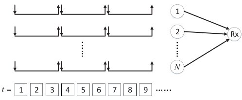
Figure 1: System model with $D=3$.

Given system parameters — the packet hard delay $D$, the number of stations $N$, and the retransmission probability $p$, we define the system timely throughput as the per-slot average number of delivered packets before expiration, i.e.,

$$R(D,N,p)\triangleq\lim_{t\to\infty}\frac{\mathbb{E}\left[\begin{subarray}{c}\text{number of packets delivered before }\\ \text{expiration from slot 1 to slot $t$}\end{subarray}\right]}{t}.$$ (1)

Our system timely throughput only counts those packets that have been delivered before expiration and ignores those packets that expire and are removed from the system after their deadlines. Sometimes $R(D,N,p)$ is simply called system throughput.

Since our traffic pattern is frame-synchronized and the retransmission probabilities of all stations are the same at all slots, it is easy to see that the average number of delivered packets before expiration is the same for all frames. Thus, we only need to focus on the first frame and the system timely throughput becomes

$$R(D,N,p)=\frac{\mathbb{E}\left[\begin{subarray}{c}\text{number of packets delivered before }\\ \text{expiration from slot 1 to slot $D$}\end{subarray}\right]}{D}.$$ (2)

Note that (2) also indicates that the limit in (1) exists, and thus (1) is well-defined.

We define the optimal retransmission probability as,

$$p^{*}(D,N)\triangleq\arg\max_{p\in(0,1]}R(D,N,p),$$ (3)

which maximizes the system throughput $R(D,N,p)$. We also denote the maximum system throughput by

$$R^{*}(D,N)\triangleq\max_{p\in(0,1]}R(D,N,p)=R(D,N,p^{*}(D,N)).$$

Let us see a special case of $D=1$. When $D=1$, every station has a new packet arrival every slot. Then the system throughput becomes

$$R(1,N,p)=\binom{N}{1}p(1-p)^{N-1}=Np(1-p)^{N-1}.$$

It is easy to see that the optimal retransmission probability is $p^{*}(1,N)=\frac{1}{N}$, and the maximum system throughput is $R^{*}(1,N)=\left(1-\frac{1}{N}\right)^{N-1}.$ Clearly, we have

$$\lim_{N\to\infty}R^{*}(1,N)=\frac{1}{e}=36.8\%,$$ (4)

which is the same as that in the delay-unconstrained slotted ALOHA with saturated traffic [12, Chapter 5.3.2] where all $N$ stations transmit/retransmit their packets with probability $p$ and each station always has a new packet arrival once its packet has been delivered successfully.

Beyond this special case of $D=1$, next we propose an algorithm to compute $R(D,N,p)$ for any hard delay $D\geq 1$ in Section III. For any $D\geq 1$, we further analyze the asymptotic performance of $p$-constant slotted ALOHA when the number of stations $N$ goes to infinity in Section IV.

III An Algorithm to Compute $R(D,N,p)$

We will show an algorithm to compute $R(D,N,p)$ in this section. Recall that we only need to focus on the first frame from slot 1 to slot $D$ (see (2)). At (the beginning of) slot 1, all $N$ stations have a new packet arrival. Random variable $M_{t}$ denotes the number of stations that have already delivered their packets (we call them finished stations) before slot $t\in\{1,2,\cdots,D\}$. Clearly $M_{1}=0$ and $M_{t}\in\{0,1,2,\cdots,\min\{t-1,N\}\}$. We also let $M_{D+1}$ denote the number of finished stations at the end of slot $D$. Note that $N-M_{t}$ is the number of active stations at (the beginning of) slot $t$ that will transmit/retransmit their packets with probability $p$ in slot $t$. Random variable $S_{t}\in\{0,1\}$ denotes the number of packets delivered successfully in slot $t\in\{1,2,\cdots,D\}$. Thus, the total number of packets delivered successfully in the first frame is $S_{1}+S_{2}+\cdots+S_{D}$. According to (2), the system throughput is

$$R(D,N,p)=\frac{\mathbb{E}[S_{1}+S_{2}+\cdots+S_{D}]}{D}=\frac{\mathbb{E}[S_{1}]+\mathbb{E}[S_{2}]+\cdots+\mathbb{E}[S_{D}]}{D}=\frac{\sum_{t=1}^{D}P(S_{t}=1)}{D}.$$ (5)

To calculate $R(D,N,p)$, we only need to calculate $P(S_{t}=1),\forall t\in\{1,2,\cdots,D\}$. Note that

$$P(S_{t}=1)=\sum_{m=0}^{\min\{t-1,N\}}P(S_{t}=1|M_{t}=m)P(M_{t}=m),$$ (6)

and

$$P(S_{t}=1|M_{t}=m)=\left\{\begin{array}[]{ll}(N-m)p(1-p)^{N-m-1},&\hbox{if $m<N$;}\\ 0,&\hbox{if $m=N$.}\end{array}\right.$$ (9)

Thus, to obtain $P(S_{t}=1)$, we only need to calculate

$$P(M_{t}=m),\quad\forall t\in\{1,2,\cdots,D\},\forall m\in\{0,1,2,\cdots,\min\{t-1,N\}\}.$$ (10)

The evolution of $M_{t}$ can be described as a trellis, as illustrated in Fig. 2 for $N=2$ and $D=4$. Based on the trellis, we can recursively calculate $P(M_{t}=m)$ as follows:

• $t=1$: $P(M_{t}=0)=P(M_{1}=0)=1.$

• For any $t\in\{1,2,\cdots,D-1\}$, based on $P(M_{t}=m)$, we calculate $P(M_{t+1}=m)$ where $m\in\{0,1,\cdots,\min\{t,N\}\}$ according to the following three cases:

  
  

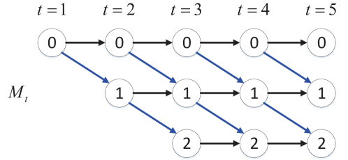
  Figure 2: The trellis describing the evolution of $M_{t}$ when $N=2$ and $D=4$. Note that we also show $M_{D+1}=M_{5}$, which is the number of finished stations at the end of slot $D$. Any blue link in the trellis corresponds to a successful delivery, implying $S_{t}=1$.

  (i) When $m=0$, we have

  $$P(M_{t+1}=m)=P(M_{t+1}=0)=\sum_{m^{\prime}=0}^{\min\{t-1,N\}}P(M_{t+1}=0|M_{t}=m^{\prime})P(M_{t}=m^{\prime})$$

  $$=P(M_{t+1}=0|M_{t}=0)P(M_{t}=0)=\left[1-Np(1-p)^{N-1}\right]P(M_{t}=0).$$ (11)

  (ii) When $m\in\{1,2,\cdots,\min\{t,N\}-1\}$, we have

  $$P(M_{t+1}=m)=\sum_{m^{\prime}=0}^{\min\{t-1,N\}}P(M_{t+1}=m|M_{t}=m^{\prime})P(M_{t}=m^{\prime})$$

  $$=P(M_{t+1}=m|M_{t}=m-1)P(M_{t}=m-1)+P(M_{t+1}=m|M_{t}=m)P(M_{t}=m)$$

  $$\leavevmode\resizebox{398.9296pt}{}{$=\left[N-(m-1)\right]p(1-p)^{N-(m-1)-1}P(M_{t}=m-1)+\left[1-(N-m)\right]p(1-p)^{N-m-1}P(M_{t}=m)$}.$$ (12)

  (iii) When $m=\min\{t,N\}$, we consider two sub-cases:

  • When $t\leq N$, we have $m=\min\{t,N\}=t$ and

    $$P(M_{t+1}=m)=P(M_{t+1}=t)=\sum_{m^{\prime}=0}^{\min\{t-1,N\}}P(M_{t+1}=t|M_{t}=m^{\prime})P(M_{t}=m^{\prime})$$

    $$=P(M_{t+1}=t|M_{t}=t-1)P(M_{t}=t-1)$$

    $$=\left[N-(t-1)\right]p(1-p)^{N-(t-1)-1}P(M_{t}=t-1).$$ (13)

  • When $t>N$, we have $m=\min\{t,N\}=N$ and

    $$P(M_{t+1}=m)=P(M_{t+1}=N)=\sum_{m^{\prime}=0}^{\min\{t-1,N\}}P(M_{t+1}=N|M_{t}=m^{\prime})P(M_{t}=m^{\prime})$$

    $$=P(M_{t+1}=N|M_{t}=N-1)P(M_{t}=N-1)+P(M_{t}=N)$$

    $$=p\cdot P(M_{t}=N-1)+P(M_{t}=N).$$ (14)

Therefore, we can first use (11)-(14) to recursively obtain (10), whose time complexity is $O(\min\{D,N\}\cdot D)$. Then we use (9) and (10) to obtain $P(S_{t}=1)$, i.e., (6), for all $t=1,2,\cdots,D$, whose time complexity is $O(\min\{D,N\}\cdot D)$. Finally, we use (5) to compute the system throughput $R(D,N,p)$, whose time complexity is $O(D)$. The overall time complexity to compute the system throughput $R(D,N,p)$ is $O(\min\{D,N\}\cdot D)$.

Now we can use this algorithm to compute $R(D,N,p)$ for any system parameters $D,N$ and $p$, and thus we can numerically obtain the optimal retransmission probability $p^{*}(D,N)$ and the maximum system throughput $R^{*}(D,N)$ (with certain step-size error).

IV Asymptotic Performance of $p$-Constant ALOHA

For $p$-constant ALOHA, we have shown that the maximum system throughput converges to $1/e$ when $D=1$ in (4). This result is the same as that in delay-unconstrained slotted ALOHA with saturated traffic. For general (fixed) $D\geq 1$, when $N$ is large, at slot 1, it has $N$ active stations that have packets to send; at slot 2, there are at least $N-1$ active stations. Similarly, at any slot $t\in\{1,2,\cdots,D\}$, there are at least $N-t+1$ active stations. Since $N-t+1\rightarrow\infty$ (as $N\rightarrow\infty$) for $1\leq t\leq D$, it is reasonable to anticipate that a similar situation to the delay-unconstrained case with saturated traffic occurs in the delay-constrained case — the number of active stations goes unbounded at all slots. According to this intuition, we conjecture that the maximum system throughput converges to $1/e=36.8\%$ for any hard delay $D$. We now present one of our main results.

Theorem 1

For any $D\geq 1$, we have $\lim_{N\to\infty}R^{*}(D,N)=1/e.$

Next we prove Theorem 1 rigourously. Towards that end, we first prove some useful lemmas.

IV-A Useful Lemmas

The optimal retransmission probability $p^{*}(D,N)$ depends on the number of stations $N$ and the packet hard delay $D$. In this section, we fix $D$ but evaluate the asymptotic performance when $N\to\infty$. For notational convenience, we drop the dependence of the retransmission probability on $D$ and let $p(N)\in(0,1]$ denote the retransmission probability when the number of stations is $N$. In the paper, we assume that all stations know $N$, and are able to choose the retransmission probability depending on $N$. In practice, when $N$ is not known a priori, there are many works to estimate $N$ based on the acknowledge information, e.g., [39, 29], which can be applied to our problem. Later, we will also propose an algorithm to estimate $N$ in Algorithm 2. For the time being, we assume that $N$ is known a priori.

Lemma 1

Consider a sequence $\{N_{k}\}$ of positive integers where $N_{1}<N_{2}<N_{3}<\cdots$, which is a subsequence of the positive-integer sequence $\{1,2,3,\cdots\}$. If the retransmission probability $p(N)$ satisfies

$$\lim_{k\to\infty}p(N_{k})=0,$$ (15)

and

$$\lim_{k\to\infty}N_{k}\cdot p(N_{k})=\delta,$$ (16)

where $\delta$ could be any non-negative real number or $\infty$, then

$$\lim_{k\to\infty}(N_{k}-A)p(N_{k})\left[1-p(N_{k})\right]^{N_{k}-B}=\frac{\delta}{e^{\delta}},$$ (17)

where $A$ and $B$ are any non-negative integers and by convention we set

$$\frac{\infty}{e^{\infty}}=0.$$ (18)

Proof:

Please see Appendix -A. ∎

Now we consider the first frame from slot 1 to slot $D$. Similar to the definition of random variable $M_{t}$ in Section III, we let random variable $M_{N,t}$ denote the number of finished stations, i.e., those stations that have already delivered their packets, before slot $t\in\{1,2,\cdots,D\}$ when the total number of stations is $N$. The reason that we introduce a new notation $M_{N,t}$ is because we need to explore its relation with respect to $N$. Clearly $M_{N,t}\in\{0,1,2,\cdots,\min\{t-1,N\}\}$. Later when we prove the sequence-limit-related statements, we consider sufficiently large $N$, e.g., $N\geq D+1$. And thus $\min\{t-1,N\}=t-1$. Then by denoting the probability of $M_{N,t}=m$ by $P(M_{N,t}=m)$, we prove the following lemma.

Lemma 2

Consider a sequence $\{N_{k}\}$ of positive integers where $N_{1}<N_{2}<N_{3}<\cdots$, which is a subsequence of the positive-integer sequence $\{1,2,3,\cdots\}$. If the retransmission probability $p(N_{k})$ satisfies (15) and (16) where $\delta$ could be any non-negative real number or $\infty$, then the sequence $\{P(M_{N_{k},t}=m)\}_{k=1}^{\infty}$ has a limit for any $t\in\{1,2,\cdots,D\}$ and any $m\in\{0,1,2,\cdots,t-1\}$. Namely, there exists a non-negative real number $\gamma_{t}^{m}$ such that

$$\lim_{k\to\infty}P(M_{N_{k},t}=m)=\gamma_{t}^{m},\forall t\in\{1,2,\cdots,D\},\forall m\in\{0,1,\cdots,t-1\}.$$ (19)

In addition,

$$\sum_{m=0}^{t-1}\gamma_{t}^{m}=1,\quad\forall t\in\{1,2,\cdots,D\}.$$ (20)

Proof:

Please see Appendix -B. ∎

We further present another preliminary lemma.

Lemma 3

Suppose that $\{a_{N}\},\{b_{N}\}$ are two bounded sequences where $b_{N}\geq 0,\forall N$. If $\limsup_{N\to\infty}a_{N}\leq 0,$ then $\limsup_{N\to\infty}a_{N}b_{N}\leq 0.$

Proof:

Please see Appendix -C. ∎

IV-B The System Throughput when $p(N)=1/N$

In this subsection, we leverage Lemma 2 to show that the system throughput goes to $1/e$ when the retransmission probability is $p(N)=1/N$.

Lemma 4

Consider the retransmission probability $p(N)=1/N$ when the number of stations is $N$. Then the system throughput converges to $1/e$, i.e.,

$$\lim_{N\to\infty}R(D,N,1/N)=1/e.$$

Proof:

Please see Appendix -D. ∎

IV-C Proof of Theorem 1

We then proceed to prove Theorem 1 when we use the optimal retransmission probability $p(N)=p^{*}(D,N)$. Since $p^{*}(D,N)$ is the optimal retransmission probability to maximize the system throughput, we have

$$R^{*}(D,N)=R(D,N,p^{*}(D,N))\geq R(D,N,1/N).$$

Thus, according to Lemma 4, we have

$$\liminf_{N\to\infty}R^{*}(D,N)\geq\liminf_{N\to\infty}R(D,N,1/N)=1/e.$$

Then Theorem 1 holds if we can verify

$$\limsup_{N\to\infty}R^{*}(D,N)\leq 1/e..$$ (21)

For any slot $t\in\{1,2,\cdots,D\}$ in the first frame, suppose that we have $M_{N,t}=m\in\{0,1,\cdots,t-1\}$ finished stations before slot $t$. Clearly, there are $N-m$ active stations that have a packet at slot $t$. Then the probability of delivering a packet in slot $t$ given that there are $m$ finished station before slot $t$ is

$$\leavevmode\resizebox{433.62pt}{}{$\alpha(N,m)=(N-m)p^{*}(N,D)\left[1-p^{*}(N,D)\right]^{N-m-1}\leq\max_{p\in(0,1]}\left[(N-m)p(1-p)^{N-m-1}\right]=\left(1-\frac{1}{N-m}\right)^{N-m-1}$},$$

where the last equality follows from the fact that

$$\arg\max_{p\in(0,1]}p(1-p)^{N-m-1}=\frac{1}{N-m}.$$

Then, we have

$$\limsup_{N\to\infty}\alpha(N,m)\leq\limsup_{N\to\infty}\left(1-\frac{1}{N-m}\right)^{N-m-1}=\frac{1}{e},$$

implying that

$$\limsup_{N\to\infty}\left[\alpha(N,m)-\frac{1}{e}\right]\leq 0.$$

Recall that we use random variable $S_{N,t}\in\{0,1\}$ to denote the number of packets delivered in slot $t$. Then, the probability of delivering a packet in slot $t$ is $P(S_{N,t}=1)$, and we have

$$P(S_{N,t}=1)-\frac{1}{e}=\sum_{m=0}^{t-1}P(S_{N,t}=1|M_{N,t}=m)P(M_{N,t}=m)-\frac{1}{e}$$

$$=\sum_{m=0}^{t-1}\alpha(N,m)P(M_{N,t}=m)-\frac{1}{e}\cdot\sum_{m=0}^{t-1}P(M_{N,t}=m)=\sum_{m=0}^{t-1}\left[\alpha(N,m)-\frac{1}{e}\right]P(M_{N,t}=m).$$

If we set $a_{N}=\alpha(N,m)-\frac{1}{e},b_{N}=P(M_{N,t}=m)$, we can see that $\{a_{N}\}$ and $\{b_{N}\}$ satisfy the conditions in Lemma 3. Hence,

$$\limsup_{N\to\infty}a_{N}b_{N}=\limsup_{N\to\infty}\left[\alpha(N,m)-\frac{1}{e}\right]P(M_{N,t}=m)\leq 0.$$

Then, we have

$$\limsup_{N\to\infty}P(S_{N,t}=1)-\frac{1}{e}=\limsup_{N\to\infty}\left[P(S_{N,t}=1)-\frac{1}{e}\right]=\limsup_{N\to\infty}\sum_{m=0}^{t-1}\left[\alpha(N,m)-\frac{1}{e}\right]P(M_{N,t}=m)$$

$$\leq\sum_{m=0}^{t-1}\left\{\limsup_{N\to\infty}\left[\alpha(N,m)-\frac{1}{e}\right]P(M_{N,t}=m)\right\}\leq\sum_{m=0}^{t-1}0=0.$$

Therefore, we have

$$\limsup_{N\to\infty}P(S_{N,t}=1)\leq\frac{1}{e}.$$

Thus, the system throughput $R^{*}(D,N)$ satisfies

$$\limsup_{N\to\infty}R^{*}(D,N)=\limsup_{N\to\infty}\frac{\sum\limits_{t=1}^{D}P(S_{N,t}=1)}{D}\leq\frac{\sum\limits_{t=1}^{D}\limsup\limits_{N\to\infty}P(S_{N,t}=1)}{D}\leq\frac{\sum\limits_{t=1}^{D}\frac{1}{e}}{D}=\frac{1}{e},$$

which proves (21). The proof for Theorem 1 is completed.

IV-D The Asymptotic Behavior of the Optimal Retransmission Probability

Theorem 1 shows that the asymptotic maximum system throughput converges to $1/e=36.8\%$ for any hard delay $D$. This is one key indicator for asymptotic performance that we hope to understand for delay-constrained slotted ALOHA. It suggests that the asymptotic maximum system throughput for delay-constrained case is the same as that for delay-unconstrained case with saturated traffic. Another indicator for asymptotic performance is how the optimal retransmission probability $p^{*}(D,N)$ changes as $N$ goes to infinity. Our Lemma 4 shows that when $p(N)=1/N$, the system throughput converges to $1/e$, which is exactly the asymptotic maximum system throughput (achieved by the optimal retransmission probability $p^{*}(D,N)$). It is thus reasonable to conjecture that $p^{*}(D,N)$ behaves as $1/N$ when $N$ is large enough. To prove our conjecture (Theorem 2), we first prove the following two lemmas.

Lemma 5

Consider a sequence $\{N_{k}\}$ of positive integers where $N_{1}<N_{2}<N_{3}<\cdots$, which is a subsequence of the positive-integer sequence $\{1,2,3,\cdots\}$. If the retransmission probability $p(N)$ satisfies (15) and (16) where $\delta$ could be any non-negative real number or $\infty$ but $\delta\neq 1$, then the limit $\lim_{k\to\infty}R(D,N_{k},p(N_{k}))$ exists and satisfies

$$\lim_{k\to\infty}R(D,N_{k},p(N_{k}))<\frac{1}{e}.$$

Proof:

Please see Appendix -E. ∎

Now we provide another lemma to show that the optimal retransmission probability converges to 0 as the number of stations goes to infinity.

Lemma 6

For any $D\geq 1$, we have $\lim\limits_{N\to\infty}p^{*}(D,N)=0.$

Proof:

Please see Appendix -F. ∎

We then prove the asymptotic performance of the optimal retransmission probability.

Theorem 2

For any $D\geq 1$, we have $\lim\limits_{N\to\infty}N\cdot p^{*}(D,N)=1.$

Proof:

We use contradiction to prove the following two results:

$$\limsup_{N\to\infty}Np^{*}(D,N)\leq 1,$$ (22)

and

$$\liminf_{N\to\infty}Np^{*}(D,N)\geq 1.$$ (23)

If both (22) and (23) hold, we have that $\lim_{N\to\infty}Np^{*}(D,N)=1$, and thus finish the proof.

Proof of (22). Suppose $\limsup_{N\to\infty}Np^{*}(D,N)>1$. Then we can find a subsequence $\{N_{k}\}_{k=1}^{\infty}$ such that

$$\lim_{k\to\infty}N_{k}p^{*}(D,N_{k})=\delta_{1}>1,$$ (24)

where $\delta_{1}$ could be $\infty$. Lemma 6 shows that $p^{*}(D,N_{k})$ satisfies (15). In addition, (24) shows that $p^{*}(D,N_{k})$ satisfies (16) with $\delta=\delta_{1}>1$. Then Lemma 5 shows that

$$\lim_{k\to\infty}R^{*}(D,N_{k})=\lim_{k\to\infty}R(D,N_{k},p^{*}(D,N_{k}))<\frac{1}{e},$$

which contradicts to Theorem 1. Thus, (22) holds.

Proof of (23). Suppose $\liminf_{N\to\infty}Np^{*}(D,N)<1$. Then we can find a subsequence $\{N_{k}\}_{k=1}^{\infty}$ such that

$$\lim_{k\to\infty}N_{k}p^{*}(D,N_{k})=\delta_{2}<1.$$

Again, from Lemma  5, we have

$$\lim_{k\to\infty}R^{*}(D,N_{k})=\lim_{k\to\infty}R(D,N_{k},p^{*}(D,N_{k}))<\frac{1}{e},$$

which contradicts to Theorem 1. Thus, (23) also holds.

The proof is completed. ∎

Theorem 2 rigorously shows that indeed the optimal retransmission probability behaves asymptotically as $1/N$. Thus, when $N$ is large enough, even though we cannot obtain the explicit formula for the optimal retransmission probability, we can simply let it be $1/N$, which simplifies the system design for $p$-constant delay-constrained slotted ALOHA.

V Two Delay-Constrained Slotted ALOHA Variants

Previous sections considered $p$-constant (delay-constrained) slotted ALOHA where the retransmission probability is the same all the time. In this section, we analyze two delay-constrained slotted ALOHA variants: $p$-dynamic slotted ALOHA and framed slotted ALOHA.

V-A $p$-dynamic Slotted ALOHA

Instead of only considering constant retransmission probability, there is another design space of dynamically changing the retransmission probability at different slots, which is called $p$-dynamic slotted ALOHA. We assume that each station knows the number of active stations (i.e., those stations with a not-yet-delivered packet) at slot $t$, which is denoted by $n(t)$.

Let $p_{\textsf{dynamic}}(n,t)$ denote the retransmission probability in slot $t$ when there are $n\geq 1$ active stations at the beginning of slot $t$. Due to the frame-synchronized structure, we only need to consider the first frame, i.e., $t=1,2,\cdots,D$. We then vectorize $p_{\textsf{dynamic}}(n_{t},t)$ as $\boldsymbol{p}=\{p_{\textsf{dynamic}}(n,t),n=1,2,\cdots,N,t=1,2,\cdots,D\}$. Note that for a given retransmission policy $\boldsymbol{p}$, we can use the similar algorithm in Section III to compute the system throughput, denoted by $R_{\textsf{dynamic}}(D,N,\boldsymbol{p})$. In addition, we are interested in finding the best retransmission policy $\boldsymbol{p}$ to maximize the system throughput, i.e.,

$$\boldsymbol{p}^{*}=\arg\max_{\boldsymbol{p}}R_{\textsf{dynamic}}(D,N,\boldsymbol{p}).$$

Similar to the analysis in Section III, we let $S_{t}\in\{0,1\}$ denote the number of packets delivered successfully in slot $t\in\{1,2,\cdots,D\}$. Then similar to (5), we can compute the system throughput, i.e.,

$$R_{\textsf{dynamic}}(D,N,\boldsymbol{p})=\frac{\sum_{t=1}^{D}P(S_{t}=1)}{D},$$

where the distribution of $S_{t}$ depends on system parameters $D$ and $N$ and the retransmission policy $\boldsymbol{p}$. Then similar to (6) and (9), we have

$$P(S_{t}=1)=\sum_{n=1}^{N}P(S_{t}=1|n(t)=n)P(n(t)=n),$$

and

$$P(S_{t}=1|n(t)=n)=n\cdot p_{\textsf{dynamic}}(n,t)\cdot\left[1-p_{\textsf{dynamic}}(n,t)\right]^{n-1}\leq\left(1-\frac{1}{n}\right)^{n-1},$$

where the inequality is achieved when

$$p_{\textsf{dynamic}}(n,t)=\frac{1}{n}.$$ (25)

Thus, among all possible retransmission policies, the one in (25) maximizes $P(S_{t}=1)$, and then maximizes the system throughput $R_{\textsf{dynamic}}(D,N,\boldsymbol{p})$. Therefore, the optimal retransmission policy $\boldsymbol{p}^{*}$ is

$$p^{*}_{\textsf{dynamic}}(n,t)=\frac{1}{n}.$$

Note that this retransmission policy is stationary for all slots. Then as we have used $n(t)$ to denote the number of active stations at slot $t$, we can rewrite the optimal retransmission policy as

$$p^{*}_{\textsf{dynamic}}(n(t))=\frac{1}{n(t)}.$$ (26)

We further let $R^{*}_{\textsf{dynamic}}(D,N)=R_{\textsf{dynamic}}(D,N,\boldsymbol{p}^{*})$ denote the maximum system throughput of $p$-dynamic slotted ALOHA. We show its asymptotic system throughput.

Theorem 3

For any $D\geq 1$,

$$\lim_{N\to\infty}R^{*}_{\textsf{dynamic}}(D,N)=\lim_{N\to\infty}R_{\textsf{dynamic}}(D,N,\boldsymbol{p}^{*})=1/e.$$ (27)

Proof:

Please see Appendix -G. ∎

Theorem 3 shows that the design space of dynamic retransmission probability cannot enlarge the asymptotic system throughput. Thus, to achieve the best asymptotic system throughput, i.e., $1/e$, it suffices to use the constant retransmission probability. Although $p$-constant slotted ALOHA and $p$-dynamic slotted ALOHA have the same asymptotic system throughput, they are different in two aspects. First, $p$-constant slotted ALOHA only needs to know the total number of stations, i.e., $N$, to compute the optimal retransmission probability $p^{*}(D,N)$ while $p$-dynamic slotted ALOHA needs to know the number of active stations at each slot, i.e, $n(t)$, to compute the optimal retransmission policy, i.e., (26). Second, $p$-constant slotted ALOHA needs to run an algorithm to compute the optimal retransmission probability $p^{*}(D,N)$ but the optimal retransmission policy of $p$-dynamic slotted ALOHA has a closed-form, i.e., (26), which simplifies the computation.

V-B Framed Slotted ALOHA

We further consider another different slotted ALOHA scheme for the frame-synchronized traffic pattern, which is called framed slotted ALOHA [20, 21, 22]. At the beginning of each frame, say the first frame, each station randomly picks up a slot, say slot $t$, according to a uniform distribution; then the station transmits its packet with probability $p$ at slot $t$, and remains idle at all other slots in this frame. Note that since each station will at most transmit once in a frame, this scheme does not require the acknowledge information of the receiver/channel, and all stations will not retransmit their packets. Random variable $S_{t}$ denotes the number of packets delivered in slot $t\in\{1,2,\cdots,D\}$. Then the system throughput is

$$R_{\textsf{framed}}(D,N,p)=\frac{\mathbb{E}[S_{1}+S_{2}+\cdots S_{D}]}{D}=\frac{\sum_{t=1}^{D}P(S_{t}=1)}{D}=P(S_{1}=1),$$

where the last equality holds because all slots will be selected by any station with equal probability, and there is no retransmission in the same frame. We let $p^{*}=\arg\max_{p\in(0,1]}R_{\textsf{framed}}(D,N,p)$ denote the optimal retransmission probability to maximize the system throughput of framed slotted ALOHA, and let $R^{*}_{\textsf{framed}}(D,N)=R_{\textsf{framed}}(D,N,p^{*})$ denote the corresponding maximum system throughput.

Note that when $D=1$, we have

$$P(S_{t}=1) =Np(1-p)^{N-1},$$

which is maximized at $p=1/N$. When $D\geq 2$, we let $N_{t}$ denote the number of stations picking up slot $t\in\{1,2,\cdots,D\}$ and thus we have

$$P(S_{t}=1)=\sum_{k=0}^{N}P(S_{t}=1|N_{t}=k)P(N_{t}=k)=\sum_{k=0}^{N}kp(1-p)^{k-1}\binom{N}{k}\left(\frac{1}{D}\right)^{k}\left(1-\frac{1}{D}\right)^{N-k}$$

$$=\leavevmode\resizebox{433.62pt}{}{$\frac{p}{1-p}\cdot\left(\frac{D-p}{D}\right)^{N}\sum_{k=0}^{N}k\binom{N}{k}\left(\frac{1-p}{D-p}\right)^{k}\left(\frac{D-1}{D-p}\right)^{N-k}=\frac{p}{1-p}\cdot\left(\frac{D-p}{D}\right)^{N}\cdot N\cdot\frac{1-p}{D-p}=\frac{pN}{D-p}\cdot\left(\frac{D-p}{D}\right)^{N}.$}$$

Taking derivative with respect to $p$ yields

$$\frac{ND}{(D-p)^{2}}\left(\frac{D-p}{D}\right)^{N}+\frac{pN}{D-p}\cdot N\left(\frac{D-p}{D}\right)^{N-1}\cdot\left(-\frac{1}{D}\right)=0,$$

which leads to

$$p^{*}=\left\{\begin{array}[]{ll}\frac{D}{N},&\hbox{if $D<N$;}\\ 1,&\hbox{otherwise.}\end{array}\right.=\min\left\{\frac{D}{N},1\right\}.$$ (28)

Note that (28) also includes $p^{*}=1/N$ for the case of $D=1$. Thus, (28) is the optimal retransmission probability of framed slotted ALOHA for any given $D$ and $N$.

Thus, when $N>D>1$, $p^{*}=D/N$ and the maximum system throughput is

(29)

which also applies to the maximum system throughput for the case of $D=1$. Thus, (29) is the maximum system throughput for any $N$ and any $D$ such that $N>D$. Note that when $N>D$, the maximum system throughput of framed slotted ALOHA is the same for any $D\geq 1$.

When $N\leq D$, $p^{*}=1$ and the maximum system throughput is

$$R^{*}_{\textsf{framed}}(D,N)=R_{\textsf{framed}}(D,N,p^{*})=R_{\textsf{framed}}(D,N,1)=\frac{N}{D-1}\cdot\left(\frac{D-1}{D}\right)^{N}.$$ (30)

Note that by convention we assume that (30) includes the case of $N=D=1$, i.e., $\frac{N}{D-1}\cdot\left(\frac{D-1}{D}\right)^{N}=\frac{N}{D-1}\cdot\frac{D-1}{D}=\frac{N}{D}=1.$ Thus, (30) works for any $D\geq 1$.

Clearly, we also have

$$\lim_{N\to\infty}R^{*}_{\textsf{framed}}(D,N)=\lim_{N\to\infty}\left(1-\frac{1}{N}\right)^{N-1}=\frac{1}{e}.$$ (31)

Thus, framed slotted ALOHA has the same asymptotic system throughput as that of $p$-constant slotted ALOHA and $p$-dynamic slotted ALOHA. However, there are several advantages of the results of framed slotted ALOHA. First, for any finite $D$ and $N$, we have the closed-form optimal retransmission probability in (28), and the closed-form maximum system throughput as shown in (29) and (30). However, in our $p$-constant slotted ALOHA, we only have an algorithm to compute $R(D,N,p)$ based on which we can numerically get the optimal retransmission probability and maximum system throughput, and in our $p$-dynamic slotted ALOHA, though we have a closed-form optimal retransmission probability, we still need to run an algorithm to compute the maximum system throughput. Second, in both $p$-constant and $p$-dynamic slotted ALOHA, the acknowledge information is required to inform the stations whether their transmissions are successful or not. However, in the framed slotted ALOHA, since each station will only transmit at most once in a frame, and all packets expire before the end of their frames, such acknowledge information is not required, which simplifies the system design.

VI A Reinforcement-Learning-Based Approach to Go Beyond $1/e$

Previous sections proved that three different delay-constrained slotted ALOHA schemes can only achieve the asymptotic timely throughput of $1/e$. The fundamental reason is that for finite $D$, the number of active stations at any slot goes to infinity as $N\to\infty$ and all active stations will join the competition with the same probability under ALOHA-based schemes. Thus, the maximum average number of packets delivered successfully in any slot is $1/e$. Therefore, the asymptotic timely throughput cannot go beyond $1/e$. In order to go beyond $1/e$, we have to reduce the competition level. The competition level can be effectively reduced by enabling active stations to cooperate with each other but still in a distributed manner without coordination. So we design a new less-aggressive random access scheme through reinforcement learning to achieve mutual cooperation among active stations. In this section, we will thoroughly introduce our proposed reinforcement-learning-based random access scheme, called RLRA-DC, which achieves much higher system timely throughput than $1/e$.

Reinforcement learning has been popularly deployed in lots of decision problems in communication systems. In the paradigm of reinforcement learning, an agent can learn a successful strategy which aims at optimizing objective function by trial-and-error iteration with the environment constantly [37]. Under our proposed random access scheme RLRA-DC, each station cannot communication with other stations so that it does not know any information about others. However, they can interact with the AP to infer the information of other stations. Specifically, at the end of a slot, the AP will broadcast an acknowledgement (ACK) to each station if it decodes a packet successfully, broadcast a negative-acknowledgement (NACK) if it receives at least two packets but does not decode it successfully (due to channel collision), and broadcast nothing if it does not receive any packet in this slot. The idea is borrowed from [31].

Normally, reinforcement learning approach is characterized by state, action and reward function. In our RLRA-DC, the state of Station $i$ at slot $t$ is defined as

$$s_{t,i}\triangleq(l_{t,i},o_{t,i}),$$ (32)

where $l_{t,i}$ is the lead time [2] of the non-delivered packet (if any) of Station $i$ at slot $t$,

$$l_{t,i}=\left\{\begin{array}[]{ll}k,&\hbox{if Station $i$ has a packet at slot $t$, which will expire in $k$ slots;}\\ 0,&\hbox{otherwise.}\end{array}\right.$$

and $o_{t,i}\in\{\textsf{BUSY},\textsf{SUCCESSFUL},\textsf{IDLE},\textsf{FAILED}\}$ is the channel observation of Station $i$ at slot $t$. Specifically, channel observation $o_{t,i}=\textsf{BUSY}$ means that Station $i$ does not transmit a packet but receives an ACK from the AP in slot $t-1$, indicating that there is only one Station $j$ ($j\neq i$) transmitting a packet in slot $t-1$. Channel observation $o_{t,i}=\textsf{SUCCESSFUL}$ means that Station $i$ transmits a packet and receives an ACK from the AP in slot $t-1$, indicating that only Station $i$ transmits a packet in slot $t-1$. Channel observation $o_{t,i}=\textsf{IDLE}$ means that Station $i$ receive nothing from the AP at the end of slot $t-1$, indicating that there is no station transmitting a packet in slot $t-1$. Channel observation $o_{t,i}=\textsf{FAILED}$ means that Station $i$ receives an NACK from the AP at the end of slot $t-1$, indicating that there is at least two stations transmitting packets in slot $t-1$ and a channel collision occurs. We remark that our model for channel observation is the same as [31]. By convention, we set $o_{1,i}=\textsf{IDLE}$.

We define $\mathcal{S}_{t,i}$ as the set of all possible system states of Station $i$ at slot $t$. We further define $\mathcal{S}_{i}$ as the set of all possible system states of Station $i$, i.e., $\mathcal{S}_{i}\triangleq\cup_{t=1}^{\infty}\mathcal{S}_{t,i}$. We remark that $\mathcal{S}_{t,i}$ may not be equal to $\mathcal{S}_{t^{\prime},i}$ when $t\neq t^{\prime}$. For example, for any $D$, $o_{1,i}=\textsf{IDLE}$ but $o_{2,i}$ could be any one in $\{\textsf{BUSY},\textsf{SUCCESSFUL},\textsf{IDLE},\textsf{FAILED}\}$. In addition, for any $D\geq 2$, $l_{2,i}$ can only be 0 or $D-1$. In other words, it is possible that $s_{t,i}$ cannot take any value in $\mathcal{S}_{i}$ for some slot $t$. For $D=1$, $l_{t,i}=1$ for any $t$ and thus we have $\left|\mathcal{S}_{i}\right|=4$. For any $D\geq 2$, we have $\left|\mathcal{S}_{i}\right|=4(D+1)$.

At slot $t$, the action of Station $i$ is denoted by $a_{t,i}$. Similar to [31], the action space of Station $i$ is defined as $\mathcal{A}_{i}\triangleq\{\textsf{TRANSMIT},\textsf{WAIT}\}$. Action $a_{t,i}=\textsf{TRANSMIT}$ means that Station $i$ transmits its packet at slot $t$, while $a_{t,i}=\textsf{WAIT}$ means that Station $i$ does not transmit a packet at slot $t$.

We define the reward function $r_{i}(s_{t,i},a_{t,i})$ of Station $i$ as

$$r_{i}(s_{t,i},a_{t,i})\triangleq 1_{\left\{o_{t,i}\in\{\textsf{BUSY},\textsf{SUCCESSFUL}\}\right\}},\forall s_{t,i}\in\mathcal{S}_{i},a_{t,i}\in\mathcal{A}_{i},$$ (33)

where $1_{\{\cdot\}}$ is the indicator function. Note that $o_{t,i}=\textsf{BUSY}$ means that Station $j$ ($j\neq i$) transmits a packet successfully in slot $t-1$, and $o_{t,i}=\textsf{SUCCESSFUL}$ means that Station $i$ transmits a packet successfully in slot $t-1$. Thus $r_{i}(s_{t,i},a_{t,i})=1$ if the system transmits a packet successfully in slot $t-1$. Note that we model the reward with “delay of gratification”.

Algorithm 1 Reinforcement-Learning-based Random Access scheme for Delay-Constrained communications (RLRA-DC) of station $i$

1:  Initialize relative value $Q_{i}(s,a)=0,\forall s\in{\mathcal{S}_{i}},\forall a\in\mathcal{A}_{i}$

2:  Initialize average reward $\rho_{i}=0$

3:  Set learning rates $\alpha_{i}=0.01,\beta_{i}=0.01$

4:  Observe the initial system state $s_{1,i}$

5:  for $t=1,2,\cdots$ do

6:     if $t\leq 4D$ then

7:        Station $i$ adopt $p$-constant ALOHA protocol with transmission probability $p_{t,i}=1/(2N)$ where $N$ is the number of stations. Namely,

$$a_{t,i}=\left\{\begin{array}[]{ll}\textsf{TRANSMIT},&\hbox{with prob. $p_{t,i}$;}\\ \textsf{WAIT},&\hbox{with prob. $1-p_{t,i}$,}\end{array}\right.$$

8:     else

9:        $a_{t,i}=\arg\max_{a\in\mathcal{A}_{i}}Q_{i}(s_{t,i},a)$

10:     end if

11:     Observe reward $r_{i}(s_{t,i},a_{t,i})$ and state $s_{t+1,i}$

12:     Update relative value as follow,

$$Q_{i}(s_{t,i},a_{t,i}) \leftarrow Q_{i}(s_{t,i},a_{t,i})+\alpha_{i}\big{(}r_{i}(s_{t,i},a_{t,i})+\max_{a}Q_{i}(s_{t+1,i},a)-Q_{i}(s_{t,i},a_{t,i})-\rho_{i}\big{)}$$

13:     Update average reward as follow,

$$\rho_{i} \leftarrow\rho_{i}+\beta_{i}\big{(}r_{i}(s_{t,i},a_{t,i})+\max_{a}Q_{i}(s_{t+1,i},a)-Q_{i}(s_{t,i},a_{t,i})-\rho_{i}\big{)}$$

14:  end for

The most-widely used reinforcement learning algorithm is Q-learning which applies to the discounted-reward case [37]. However, the objective in our problem, i.e., the system timely throughput, is an average reward as defined in (2). Thus, motivated by [33], we think that Q-learning is less suitable to R-learning, a less-popular reinforcement learning algorithm, which applies to the average-reward case [35, 36, 37].

In this paper, we adopt the variants of R-learning in [36, Algorithm 3] and [37, Figure 11.2]. For any Station $i$, the iterations of relative value $Q_{i}(s_{t,i},a_{t,i})$ and average reward $\rho$ are as follows,

$$Q_{i}(s_{t,i},a_{t,i}) \leftarrow Q_{i}(s_{t,i},a_{t,i})+\alpha_{i}\big{(}r_{i}(s_{t,i},a_{t,i})+\max_{a\in\mathcal{A}_{i}}Q_{i}(s_{t+1,i},a)-Q_{i}(s_{t,i},a_{t,i})-\rho_{i}\big{)},$$ (34)

$$\rho_{i} \leftarrow\rho_{i}+\beta_{i}\big{(}r_{i}(s_{t,i},a_{t,i})+\max_{a\in\mathcal{A}_{i}}Q_{i}(s_{t+1,i},a)-Q_{i}(s_{t,i},a_{t,i})-\rho_{i}\big{)},$$ (35)

where $\alpha_{i}\in(0,1]$ and $\beta_{i}\in(0,1]$ are learning rates, $\rho_{i}$ approximates the state-independent average reward for the iteratively updated policy $\pi$, i.e.,

$$\rho_{i}\approx\lim_{T\to\infty}\mathbb{E}^{\pi}\left[\frac{\sum_{t=1}^{T}r_{i}(s_{t,i},a_{t,i})}{T}\right],$$ (36)

and Q-function $Q_{i}(s_{t,i},a_{t,i})$ approximates the state-dependent cumulative reward difference (called relative value in [36, 37]) for the iteratively updated policy $\pi$, i.e.,

$$Q_{i}(s_{t,i}=s,a_{t,i}=a)\approx\mathbb{E}^{\pi}\left[\left.\sum_{\tau=t}^{\infty}\left[r_{i}(s_{\tau,i},a_{\tau,i})-\rho_{i}\right]\right|s_{t,i}=s,a_{t,i}=a\right].$$ (37)

Specifically, our proposed algorithm is called Reinforcement-Learning-based Random Access scheme for Delay-Constrained communications (RLRA-DC) of station $i$ for a given number of station, i.e., $N$, as shown in Algorithm 1.

As we can see in Algorithm 1, in the first $4D$ slots (which is a short period), each station adopts $p$-constant slotted ALOHA protocol with transmission probability $1/(2N)$ (which is a small value) to initialize its Q-table. The goal of this procedure is to create some heterogeneity of initialized policies of all stations. Furthermore, the small transmission probability $1/(2N)$ reduces the collision probability during the initialization period (from slot 1 to slot $4D$). In other words, we essentially pre-allocate a part of spectrum resources to a part of stations in the first $4D$ slots, which benefits the convergence of the algorithm. And the rest of spectrum resources will be allocated judiciously in later slots through the interaction between stations. We will show the superior performance of Algorithm 1 in Fig. 5.

Algorithm 2 The method of Station $i$ to estimate the number of stations, i.e., $N$

1:  Initialize a constant $p=\frac{1}{10}$

2:  for $k=1,2,\cdots,100$ do

3:     for $t=1,2,\cdots,100$ do

4:        Station $i$ adopts $p$-constant ALOHA protocol with transmission probability $p_{t}=\frac{p}{k}$

5:     end for

6:     Calculate the empirical timely throughput $R(k)$ from slot $100(k-1)+1$ to $100k$

7:  end for

8:  The estimation of station $i$ for the number of stations is $N=\frac{\arg\max_{k\in\{1,2,\cdots,100\}}R(k)}{p}$

Similar to $p$-constant slotted ALOHA and framed slotted ALOHA , Algorithm 1 again requires that $N$ is known a priori, which is sometimes difficult to be obtained in practice. Hence, we also propose a simple but practical method to estimate $N$. The idea is inspired by Theorem 2 in ALOHA system, which shows that the optimal transmission probability behaves asymptotically as $1/N$. We assume that the number of stations $N$ in the network is not larger than 1,000. The algorithm to estimate the number of stations $N$ is shown in Algorithm 2, whose effectiveness will be demonstrated in Section VII.

VII Simulation

In this section, we first confirm our theoretical analysis by simulations for the three delay-constrained slotted ALOHA schemes in Section VII-A, and then demonstrate the asymptotic performance of ALOHA-based schemes and RLRA-DC in Section VII-B and Section VII-C, respectively.

VII-A Confirmation of Theoretical Analysis for System Throughput

We first confirm our theoretical analysis for $p$-constant slotted ALOHA, $p$-dynamic slotted ALOHA, and framed slotted ALOHA. For $p$-constant slotted ALOHA (resp. $p$-dynamic slotted ALOHA), we can use our algorithm in Section III to compute the system throughput $R(D,N,p)$ (resp. $R_{\textsf{dynamic}}(D,N,\boldsymbol{p})$) for any given hard delay $D$, number of stations $N$, retransmission probability $p$ (resp. retransmission policy $\boldsymbol{p}=(p(n,t):n=1,2,\cdots,N,t=1,2,\cdots,D)$). In this simulation, we consider the dynamic retransmission policy $p(t)=\alpha/n(t)$ where $\alpha$ is a constant ranging from 0 to 2, and $n(t)$ is the number of active stations at the beginning of slot $t$. The reason that we set $p(t)=\alpha/n(t)$ is because we aim to verify that the optimal system throughput is achieved when $\alpha=1$ and also to check the variation of the system throughput due to $\alpha$. For framed slotted ALOHA, we have a closed form for the system throughput $R_{\textsf{framed}}(D,N,p)$ as shown in (29) and (30). Thus, for all three schemes, we can get the theoretical system throughput. To verify the correctness, we further simulate a real system for the three schemes and obtain the empirical system throughput. We fix hard delay $D=10$ and consider $N=5,10,$ and $15$ and simulate these three schemes for 10,000 frames (of in total 100,000 slots) to obtain the empirical system throughput. The results are shown in Fig. 3.

For all three ALOHA-based schemes, as expected, we can see that the theoretical system throughput is the same as the empirical system throughput, which confirms our theoretical derivation for system throughput for all three schemes. From the middle figure in Fig. 3 for $p$-dynamic slotted ALOHA, we can see that the system throughput is indeed maximized at $\alpha=1$, which confirms the optimal retransmission policy in (26). From the right-hand-side figure in Fig. 3 for framed slotted ALOHA, we can see that the optimal retransmission probability is $\min\{D/N,1\}$, which confirms (28).

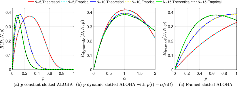
Figure 3: The system throughput of $p$-constant slotted ALOHA, $p$-dynamic slotted ALOHA, and framed slotted ALOHA with $D=10$.

VII-B Asymptotic Performance of ALOHA-based Schemes

We consider $D=10$ and show the asymptotic performance of maximum system throughput of three schemes and the asymptotic performance of the optimal retransmission probability of $p$-constant slotted ALOHA in Fig. 4. First, from Fig. 4(a), we can see that indeed the maximum system throughput of all three schemes converges to $1/e$, which confirms Theorem 1, Theorem 3, and (31). Second, to better compare three schemes, Fig. 4(b) shows the maximum system throughput of all three schemes when $N$ ranges from 1 to 15. We can see that in terms of maximum system throughput, $p$-dynamic slotted ALOHA has the best performance for any $N$; $p$-constant slotted ALOHA is better than framed slotted ALOHA when $N\leq 8$ but worse than framed slotted ALOHA when $N\geq 9$ (though with very close performance). Finally, from Fig. 4(c), we can see that indeed the optimal retransmission probability of $p$-constant slotted ALOHA behaves asymptotically as $1/N$, which verifies Theorem 2.

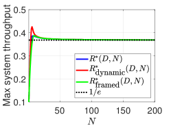
(a) Maximum system throughput of three ALOHA-based schemes.

(b) A Small range of $N$ (from 1 to 15) for Fig. 4(a).

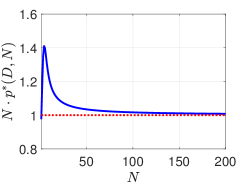
(c) Optimal retransmission prob. of $p$-constant slotted ALOHA.

Figure 4: The asymptotic performance of the maximum system throughput for three ALOHA-based schemes and the asymptotic performance of the optimal retransmission probability of $p$-constant slotted ALOHA when $D=10$.

VII-C Asymptotic Performance of RLRA-DC

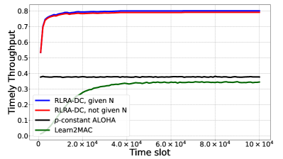
(a) The timely throughput of the 10-user case.

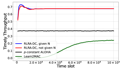
(b) The timely throughput of the 50-user case.

(c) The timely throughput of the 100-user case.

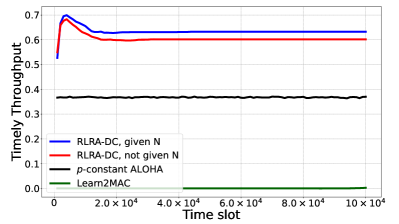
(d) The timely throughput of the 1000-user case.

Figure 5: The system timely throughput of four random access schemes when $D=10$ and $N=$ 10, 50, 100, and 1,000, respectively.

Finally, we demonstrate the superior performance of our proposed RLRA-DC described in Section VI. We set the deadline $D=10$, and the number of stations $N$ to be 10, 50, 100, and 1,000, respectively. For each $N$, we independently run 100 instances with different random seeds ranging from 1 to 100. In each instance, we run 100,000 slots and get the system timely throughput. We then average the system timely throughput of these 100 instances as the result. The baselines are the online-learning-based algorithm called Learn2MAC [34] and $p$-constant slotted ALOHA. The system timely throughput of these random access schemes are shown in Fig. 5.

From Fig. 5, we have the following four observations. First, our RLRA-DC with given $N$ always achieves the highest system timely throughput in each case, which is much larger than $1/e$. Second, when $N$ is not given, by using our proposed method to estimate the number of station in Algorithm 2, the system timely throughput of RLRA-DC is very close to that of the case when $N$ is given. It demonstrates that our estimation method in Algorithm 2 is efficient despite its simplicity. Third, the system timely throughput of $p$-constant slotted ALOHA converges to $1/e$ which is consistent with our previous sections. And the system timely throughput of Learn2MAC is even lower than that of $p$-constant slotted ALOHA. The reason is that Learn2MAC only works in the less-congested scenarios, as mentioned in [34]. Finally, as $N$ increases, the collision probability also increases, which will reduce the system timely throughput. Nevertheless, even when the number of stations $N$ increases to $1,000$, the system timely throughput of our RLRA-DC is $0.6$, which is much higher than $1/e$. Our independent simulation shows that the system timely throughput of up to 10,000 stations is also very close to 0.6, much higher than $1/e$.

Thus, Fig. 5 shows the superior performance of our proposed R-learning-based random access scheme RLRA-DC. Its system timely throughput can be much larger than $1/e$, which is the ceiling of delay-constrained ALOHA schemes.

VIII Conclusion

In this paper, we have firstly analyzed the asymptotic performance of three delay-constrained slotted ALOHA schemes under the frame-synchronized traffic pattern. We have proved that the maximum system throughput of all three schemes converges to $1/e$ when the number of stations goes to infinity. We have also characterized the optimal retransmission probability of three schemes. Then we have proposed a reinforcement-learning-based random access scheme for delay-constrained communications called RLRA-DC, whose the system timely throughput is much larger than $1/e$. In the future, to capture more practical scenarios, it is interesting to further study the delay-constrained communication under non-frame-synchronized traffic patterns. In addition, it is also important to investigate the performance of other medium access schemes, e.g., CSMA, under delay-constrained setting.

-A Proof of Lemma 1

We consider two cases: $\delta<\infty$, and $\delta=\infty$.

Case I: $\delta<\infty$. In this case, due to (15) and (16), we have

$$\lim\limits_{k\to\infty}(N_{k}-A)p(N_{k})\left[1-p(N_{k})\right]^{N_{k}-B}=\lim\limits_{k\to\infty}(N_{k}-A)p(N_{k})\cdot\lim\limits_{k\to\infty}\left[1-p(N_{k})\right]^{N_{k}}\cdot\lim\limits_{k\to\infty}\frac{1}{[1-p(N_{k})]^{B}}$$

$$=\delta\cdot\lim_{k\to\infty}\exp\left\{N_{k}\ln\left[1-p(N_{k})\right]\right\}\cdot 1=\delta\cdot\exp\left\{\lim_{k\to\infty}N_{k}\ln\left[1-p(N_{k})\right]\right\}$$

$$=\delta\cdot\exp\left\{\lim_{k\to\infty}N_{k}p(N_{k})\cdot\frac{\ln\left[1-p(N_{k})\right]}{p(N_{k})}\right\}=\delta\cdot\exp\left\{\lim_{k\to\infty}N_{k}p(N_{k})\cdot\lim_{k\to\infty}\frac{\ln\left[1-p(N_{k})\right]}{p(N_{k})}\right\}$$

$$\overset{(\text{let }u=p(N_{k}))}{=}\delta\cdot\exp\left\{\delta\cdot\lim_{u\to 0}\frac{\ln(1-u)}{u}\right\}=\delta\cdot\exp\left\{\delta\cdot\lim_{u\to 0}\frac{-\frac{1}{1-u}}{1}\right\}\quad(\text{by L'Hospital's Rule})$$

$$=\delta\cdot\exp(-\delta)=\frac{\delta}{e^{\delta}}.$$

Thus, (17) holds when $\delta<\infty$.

Case II: $\delta=\infty$. In this case, we have

$$\leavevmode\resizebox{398.9296pt}{}{$0\leq N_{k}p(N_{k})[1-p(N_{k})]^{N_{k}}=N_{k}p(N_{k})\left\{\left[1-p(N_{k})\right]^{\frac{1}{p(N_{k})}}\right\}^{N_{k}p(N_{k})}\leq N_{k}p(N_{k})\left(\frac{1}{e}\right)^{N_{k}p(N_{k})}=\frac{N_{k}p(N_{k})}{e^{N_{k}p(N_{k})}}$},$$ (38)

where the last inequality follows from the fact that

$$(1-x)^{\frac{1}{x}}<\frac{1}{e},\forall x\in(0,1].$$

Since $\lim_{k\to\infty}N_{k}p(N_{k})=\delta=\infty$, by letting $u=N_{k}p(N_{k})$, we have

$$\lim_{k\to\infty}\frac{N_{k}p(N_{k})}{e^{N_{k}p(N_{k})}}=\lim_{u\to\infty}\frac{u}{e^{u}}=0.$$

Thus, by applying the squeeze theorem to (38), we have

$$\lim_{k\to\infty}N_{k}p(N_{k})[1-p(N_{k})]^{N_{k}}=0.$$ (39)

Note that (39) implies

$$\lim_{k\to\infty}p(N_{k})[1-p(N_{k})]^{N_{k}}=0.$$ (40)

Combining (39) and (40), we have

$$\lim_{k\to\infty}(N_{k}-A)p(N_{k})\left[1-p(N_{k})\right]^{N_{k}-B}=\lim_{k\to\infty}(N_{k}-A)p(N_{k})\left[1-p(N_{k})\right]^{N_{k}}\cdot\lim_{k\to\infty}\frac{1}{[1-p(N_{k})]^{B}}$$

$$=\lim\limits_{k\to\infty}(N_{k}-A)p(N_{k})\left[1-p(N_{k})\right]^{N_{k}}\cdot 1=\lim\limits_{k\to\infty}N_{k}p(N_{k})\left[1-p(N_{k})\right]^{N_{k}}-A\cdot\lim\limits_{k\to\infty}p(N_{k})\left[1-p(N_{k})\right]^{N_{k}}$$

$$=0-A\cdot 0=0=\frac{\infty}{e^{\infty}}=\frac{\delta}{e^{\delta}},$$

where the second last equality uses the convention (18). Thus, (17) holds when $\delta=\infty$.

Case I and Case II complete the proof.

-B Proof of Lemma 2

We prove the existence of the limit (i.e., (19)) by induction with respect to $t$. Clearly, when $t=1$,

$$P(M_{N,1}=0)=1,\quad\forall N.$$

Thus,

$$\lim_{k\to\infty}P(M_{N_{k},1}=0)=1\triangleq\gamma_{1}^{0}.$$

For $t\in\{1,2,\cdots,D-1\}$, suppose that $\lim_{k\to\infty}P(M_{N_{k},t}=m)$ exists for any $m$, i.e.,

$$\lim_{k\to\infty}P(M_{N_{k},t}=m)=\gamma_{t}^{m},\quad m\in\{0,1,\cdots,t-1\}.$$

We then consider $t+1$. For $m=0$,

$$P(M_{N_{k},t+1}=m)=P(M_{N_{k},t+1}=0)=\sum_{m^{\prime}=0}^{t-1}P(M_{N_{k},t+1}=0|M_{N_{k},t}=m^{\prime})P(M_{N_{k},t}=m^{\prime})$$

$$\leavevmode\resizebox{398.9296pt}{}{$=P(M_{N_{k},t+1}=0|M_{N_{k},t}=0)P(M_{N_{k},t}=0)=\left\{1-N_{k}p(N_{k})\left[1-p(N_{k})\right]^{N_{k}-1}\right\}P(M_{N_{k},t}=0)$}.$$ (41)

Since $p(N_{k})$ satisfies (15) and (16), according to Lemma 1 where we set $A=0,B=1$, we have

$$\lim_{k\to\infty}N_{k}p(N_{k})\left[1-p(N_{k})\right]^{N_{k}-1}=\frac{\delta}{e^{\delta}}.$$

Therefore, taking limit in (41), we have

$$\leavevmode\resizebox{398.9296pt}{}{$\lim\limits_{k\to\infty}P(M_{N_{k},t+1}=0)=\lim\limits_{k\to\infty}\left\{1-N_{k}p(N_{k})\left[1-p(N_{k})\right]^{N_{k}-1}\right\}\cdot\lim\limits_{k\to\infty}P(M_{N_{k},t}=0)=\left(1-\frac{\delta}{e^{\delta}}\right)\cdot\gamma_{t}^{0}\triangleq\gamma_{t+1}^{0}$}.$$ (42)

Thus, the limit $\lim_{k\to\infty}P(M_{N_{k},t+1}=0)$ exists.

Similarly, for any $m\in\{1,2,\cdots,t-1\}$, we have

$$P(M_{N_{k},t+1}=m)=\sum_{m^{\prime}=0}^{t-1}P(M_{N_{k},t+1}=m|M_{N_{k},t}=m^{\prime})P(M_{N_{k},t}=m^{\prime})$$

$$=P(M_{N_{k},t+1}=m|M_{N_{k},t}=m-1)P(M_{N_{k},t}=m-1)+P(M_{N_{k},t+1}=m|M_{N_{k},t}=m)P(M_{N_{k},t}=m)$$

According to Lemma 1, we have

$$\lim_{k\to\infty}P(M_{N_{k},t+1}=m)=\frac{\delta}{e^{\delta}}\cdot\gamma_{t}^{m-1}+\left(1-\frac{\delta}{e^{\delta}}\right)\gamma_{t}^{m}\triangleq\gamma_{t+1}^{m}.$$

Finally, for $m=t$, we have

$$P(M_{N_{k},t+1}=t) =P(M_{N_{k},t+1}=t|M_{N_{k},t}=t-1)P(M_{N_{k},t}=t-1)$$

$$=[N_{k}-(t-1)]p(N_{k})[1-p(N_{k})]^{N_{k}-(t-1)-1}P(M_{N_{k},t}=t-1),$$

and

$$\lim_{N\to\infty}P(M_{N_{k},t+1}=t)=\frac{\delta}{e^{\delta}}\cdot\gamma_{t}^{t-1}\triangleq\gamma_{t+1}^{t}.$$

Therefore, the limit $\lim\limits_{N\to\infty}P(M_{N_{k},t+1}=m)$ exists for any $m\in\{0,1,2,\cdots,t\}$, which completes the induction proof. Thus, (19) holds.

To prove (20), we can simply take limit in both sides of the following equality,

$$\sum_{m=0}^{t-1}P(M_{N_{k},t}=m)=1,\forall t\in\{1,2,\cdots,D\}.$$

The proof is completed.

-C Proof of Lemma 3

We prove this lemma by contradiction. Suppose that it is not true. Then, since $\{a_{N}b_{N}\}$ is a bounded sequence, there exists a $\phi>0$ such that $\limsup_{N\to\infty}a_{N}b_{N}=\phi$, which implies that there exists a subsequence $\{N_{k}\}_{k=1}^{\infty}$ such that $\lim_{k\to\infty}a_{N_{k}}b_{N_{k}}=\phi>0$. Thus, there exists a $k_{0}\geq 1$ such that

$$a_{N_{k}}b_{N_{k}}>\frac{\phi}{2},\quad\forall k\geq k_{0}.$$

Since $b_{N}\geq 0,\forall n$ and it is upper bounded, say $U>0$, we have

$$a_{N_{k}}>\frac{\phi}{2U},\quad\forall k\geq k_{0},$$

which implies that

$$\limsup_{k\to\infty}a_{N_{k}}\geq\frac{\phi}{2U}>0.$$

Then we have

$$\limsup_{N\to\infty}a_{N}\geq\limsup_{k\to\infty}a_{N_{k}}>0,$$

which contradicts with $\limsup_{N\to\infty}a_{N}\leq 0$.

Therefore, we must have $\limsup_{N\to\infty}a_{N}b_{N}\leq 0$.

-D Proof of Lemma 4

Again, we consider the first frame from slot 1 to slot $D$. For any slot $t\in\{1,2,\cdots,D\}$, recall that we use random variable $M_{N,t}$ to denote the number of finished stations before slot $t$. We then let random variable $S_{N,t}\in\{0,1\}$ denote the number of packets delivered in slot $t$. Then, the probability of delivering a packet in slot $t$ is

$$P(S_{N,t}=1) =\sum\limits_{m=0}^{t-1}P(S_{N,t}=1|M_{N,t}=m)P(M_{N,t}=m)$$

$$=\sum\limits_{m=0}^{t-1}(N-m)p(N)\left[1-p(N)\right]^{N-m-1}P(M_{N,t}=m).$$

We consider the sequence $\{N_{k}\}=\{1,2,3,\cdots\}$. Then $p(N)=1/N$ satisfies (15) and (16) with $\delta=1$. Thus, according to (17) in Lemma 1 and (19) and (20) in Lemma 2, we get

$$\lim_{N\to\infty}P(S_{N,t}=1)=\lim\limits_{N\to\infty}\left\{\sum\limits_{m=0}^{t-1}(N-m)p(N)\left[1-p(N)\right]^{N-m-1}P(M_{N,t}=m)\right\}$$

$$=\sum\limits_{m=0}^{t-1}\left\{\lim\limits_{N\to\infty}(N-m)p(N)\left[1-p(N)\right]^{N-m-1}P(M_{N,t}=m)\right\}$$

$$=\sum\limits_{m=0}^{t-1}\left\{\lim\limits_{N\to\infty}(N-m)p(N)\left[1-p(N)\right]^{N-m-1}\cdot\lim\limits_{N\to\infty}P(M_{N,t}=m)\right\}$$

$$=\sum_{m=0}^{t-1}\frac{\delta}{e^{\delta}}\cdot\gamma_{t}^{m}=\frac{1}{e^{1}}\cdot\sum_{m=0}^{t-1}\gamma_{t}^{m}=\frac{1}{e}\cdot 1=\frac{1}{e}.$$

Therefore, when $N$ goes to infinity, the probability of delivering a packet in any slot $t$ is $1/e$. Thus, the system throughput also converges to $1/e$, i.e.,

$$\lim_{N\to\infty}R(D,N,1/N)=\lim_{N\to\infty}\frac{\sum_{t=1}^{D}P(S_{N,t}=1)}{D}=1/e,$$

which completes the proof.

-E Proof of Lemma 5

For any slot $t\in\{1,2,\cdots,D\}$ in the first frame, suppose that we have $M_{N_{k},t}=m\in\{0,1,\cdots,t-1\}$ finished stations before slot $t$. Clearly, there are $N_{k}-m$ active stations that have a packet at slot $t$. In addition, based on Lemma  2, we have that $\lim_{k\to\infty}P(M_{N_{k},t}=m)=\gamma_{t}^{m}$ and $\sum_{m=0}^{t-1}\gamma_{t}^{m}=1$.

Recall that we use random variable $S_{N_{k},t}\in\{0,1\}$ to denote the number of packets delivered in slot $t$. Then, the probability of delivering a packet in slot $t$ is $P(S_{N_{k},t}=1)$, and we have

$$\lim_{k\to\infty}P(S_{N_{k},t}=1)=\lim_{k\to\infty}\sum_{m=0}^{t-1}P(S_{N_{k},t}=1|M_{N_{k},t}=m)P(M_{N_{k},t}=m)$$

$$=\sum_{m=0}^{t-1}\gamma_{t}^{m}\cdot\lim_{k\to\infty}(N_{k}-m)p(N_{k})[1-p(N_{k})]^{N_{k}-m-1}=\sum_{m=0}^{t-1}\gamma_{t}^{m}\cdot\frac{\delta}{e^{\delta}}=\frac{\delta}{e^{\delta}}<1/e,$$ (43)

where the last inequality follows from the fact that $\delta\neq 1$ and the fact that function $f(x)=\frac{x}{e^{x}}$ is maximized only when $x=1$. Therefore,

$$\lim_{k\to\infty}R(D,N_{k},p(N_{k})) =\lim_{k\to\infty}\frac{\sum_{t=1}^{D}P(S_{N,t}=1)}{D}=\frac{\delta}{e^{\delta}}<1/e,$$

which completes the proof.

-F Proof of Lemma 6

Since $p^{*}(D,N)>0$, we have $\liminf\limits_{N\to\infty}p^{*}(D,N)\geq 0$. Now we only need to show $\limsup\limits_{N\to\infty}p^{*}(D,N)=0$. Let us prove this by contradiction. Suppose that

$$\limsup_{N\to\infty}p^{*}(D,N)=\phi>0.$$

This suggests that there exists a subsequence of sequence $\{N\}_{N=1}^{\infty}$, denoted by $\{N_{k}\}_{k=1}^{\infty}$, such that

$$\lim_{k\to\infty}p^{*}(D,N_{k})=\phi.$$

This further shows that there exists a $k_{0}\geq 1$ such that

$$p^{*}(D,N_{k})\geq\frac{\phi}{2}>0,\quad\forall k\geq k_{0}.$$

Let us consider $N_{k}$ stations where $N_{k}\geq\max\{N_{k_{0}},\left\lceil\frac{2}{\phi}\right\rceil+D+1\}$. At any slot $t\in\{1,2,\cdots,D\}$, suppose that there are $M_{N,t}=m$ finished stations before slot $t$. Clearly, $m\in\{0,1,2,\cdots,t-1\}$. The probability of delivering a packet in slot $t$ is

$$(N_{k}-m)p^{*}(D,N_{k})\left[1-p^{*}(D,N_{k})\right]^{N_{k}-m-1}.$$

We consider the following function

$$f(p)=(N_{k}-m)p(1-p)^{N_{k}-m-1},\quad p\in\left[\frac{\phi}{2},1\right),$$

Then,

$$\frac{df(p)}{dp}=(N_{k}-m)(1-p)^{N_{k}-m-2}[1-(N_{k}-m)p].$$

Since $N_{k}\geq\max\{N_{k_{0}},\left\lceil\frac{2}{\phi}\right\rceil+D+1\}$ and $p\in\left[\frac{\phi}{2},1\right)$, we have $N_{k}-m\geq N_{k}-D>0$ and

$$1-(N_{k}-m)p\leq 1-(N_{k}-D)\frac{\phi}{2}\leq 1-\left(\left\lceil\frac{2}{\phi}\right\rceil+1\right)\frac{\phi}{2}\leq-\frac{\phi}{2}<0.$$

Thus, for $\phi/2\leq p<1$,

$$\frac{df(p)}{dp}<0.$$

In addition, since $N_{k}\geq N_{k_{0}}$, we have $p^{*}(D,N_{k})\geq\phi/2,\forall k\geq k_{0}$. Then, we have

$$0 \leq f(p^{*}(D,N_{k}))=(N_{k}-m)p^{*}(D,N_{k})\left[1-p^{*}(D,N_{k})\right]^{N_{k}-m-1}$$

$$\leq f(\phi/2)=(N_{k}-m)\frac{\phi}{2}\left(1-\frac{\phi}{2}\right)^{N_{k}-m-1},\forall k\geq k_{0}$$ (44)

Note that

$$\lim_{k\to\infty}(N_{k}-m)\frac{\phi}{2}\left(1-\frac{\phi}{2}\right)^{N_{k}-m-1}=0.$$

Thus, by applying the squeeze theorem to (44), we have

$$\lim_{k\to\infty}(N_{k}-m)p^{*}(D,N_{k})\left[1-p^{*}(D,N_{k})\right]^{N_{k}-m-1}=0.$$

Therefore, the probability of delivering a packet in slot $t$ converges as

$$\lim_{k\to\infty}P(S_{N_{k},t}=1)=\lim_{k\to\infty}\sum_{m=0}^{t-1}P(S_{N_{k},t}=1|M_{N_{k},t}=m)P(M_{N_{k},t}=m)$$

$$=\lim\limits_{k\to\infty}\sum\limits_{m=0}^{t-1}(N_{k}-m)p^{*}(D,N_{k})\left[1-p^{*}(D,N_{k})\right]^{N_{k}-m-1}P(M_{N_{k},t}=m)$$

$$=\sum\limits_{m=0}^{t-1}\lim\limits_{k\to\infty}(N_{k}-m)p^{*}(D,N_{k})\left[1-p^{*}(D,N_{k})\right]^{N_{k}-m-1}P(M_{N_{k},t}=m)=\sum_{m=0}^{t-1}0=0,$$

where the second last equality follows from the fact that if $\lim_{n\to\infty}a_{n}=0$ and $\{b_{n}\}$ is bounded (here we have $|P(M_{N_{k},t},=m)|\leq 1$), then $\lim_{n\to\infty}a_{n}b_{n}=0$. Thus, in any slot of a frame, the probability of delivering a packet converges to 0 (under the subsequence $\{N_{k}\}$), yielding to

$$\lim_{k\to\infty}R^{*}(D,N_{k})=\lim_{k\to\infty}\frac{\sum_{t=1}^{D}P(S_{N_{k},t}=1)}{D}=0,$$

which contradicts to Theorem 1. This completes the proof.

-G Proof of Theorem 3

By following the similar induction steps in the proof of Lemma 2, it is straightforward to show that (19) and (20) hold under the optimal retransmission policy $\boldsymbol{p}^{*}=\{p^{*}_{\textsf{dynamic}}(n,t),n=1,2,\cdots,N,t=1,2,\cdots,D\}$.

Then, according to (5), we have

$$\lim_{N\to\infty}R_{\textsf{dynamic}}(D,N,\boldsymbol{p}^{*})=\frac{\sum_{t=1}^{D}\lim_{N\to\infty}P(S_{t}=1)}{D}.$$

In addition,

$$\lim_{N\to\infty}P(S_{t}=1)=\lim\limits_{N\to\infty}\sum\limits_{m=0}^{t-1}P(S_{t}=1|M_{N,t-1}=m)P(M_{N,t-1}=m)$$

$$=\lim\limits_{N\to\infty}\sum\limits_{m=0}^{t-1}(N-m)p_{\textsf{dynamic}}^{*}(N-m,t)\left[1-p_{\textsf{dynamic}}^{*}(N-m,t)\right]^{N-m-1}P(M_{N,t}=m)$$

$$=\lim\limits_{N\to\infty}\sum\limits_{m=0}^{t-1}(N-m)\frac{1}{N-m}\left(1-\frac{1}{N-m}\right)^{N-m-1}P(M_{N,t}=m)$$

$$=\sum_{m=0}^{t-1}\lim\limits_{N\to\infty}\left(1-\frac{1}{N-m}\right)^{N-m-1}\cdot\lim\limits_{N\to\infty}P(M_{N,t}=m)=\sum_{m=0}^{t-1}\frac{1}{e}\cdot\gamma_{t}^{m}=\frac{1}{e}\cdot\sum_{m=0}^{t-1}\gamma_{t}^{m}=\frac{1}{e}\cdot 1=\frac{1}{e}.$$

Thus,

$$\lim_{N\to\infty}R_{\textsf{dynamic}}(D,N,\boldsymbol{p}^{*})=\frac{\sum\limits_{t=1}^{D}\lim\limits_{N\to\infty}P(S_{t}=1)}{D}=\frac{\sum\limits_{t=1}^{D}\frac{1}{e}}{D}=\frac{1}{e}.$$

References

- [1] L. Deng, J. Deng, P.-N. Chen, and Y. S. Han, “On the asymptotic performance of delay-constrained slotted ALOHA,” in Proc. IEEE ICCCN, 2018, pp. 1–8.
- [2] L. Deng, C.-C. Wang, M. Chen, and S. Zhao, “Timely wireless flows with general traffic patterns: Capacity region and scheduling algorithms,” IEEE/ACM Transactions on Networking, vol. 25, no. 6, pp. 3473–3486, 2017.
- [3] G. P. Fettweis, “The tactile Internet: Applications and challenges,” IEEE Vehicular Technology Magazine, vol. 9, no. 1, pp. 64–70, 2014.
- [4] M. Simsek, A. Aijaz, M. Dohler, J. Sachs, and G. Fettweis, “5G-enabled tactile Internet,” IEEE Journal on Selected Areas in Communications, vol. 34, no. 3, pp. 460–473, 2016.
- [5] J. Baillieul and P. J. Antsaklis, “Control and communication challenges in networked real-time systems,” Proceedings of the IEEE, vol. 95, no. 1, pp. 9–28, 2007.
- [6] Z. Jiang, H. Cheng, Z. Zheng, X. Zhang, X. Nie, W. Li, Y. Zou, and W. S. Wong, “Autonomous formation flight of UAVs: Control algorithms and field experiments,” in Proc. CCC, 2016, pp. 7585–7591.
- [7] K. Kang, K.-J. Park, L. Sha, and Q. Wang, “Design of a crossbar VOQ real-time switch with clock-driven scheduling for a guaranteed delay bound,” Real-Time Systems, vol. 49, no. 1, pp. 117–135, 2013.
- [8] P. Popovski, J. J. Nielsen, C. Stefanovic, E. de Carvalho, E. Strom, K. F. Trillingsgaard, A.-S. Bana, D. M. Kim, R. Kotaba, J. Park, and R. B. Sorensen, “Wireless access for ultra-reliable low-latency communication: Principles and building blocks,” IEEE Network, vol. 32, no. 2, pp. 16–23, 2018.
- [9] P.-C. Hsieh and I.-H. Hou, “A decentralized medium access protocol for real-time wireless ad hoc networks with unreliable transmissions,” in Proc. IEEE ICDCS, 2018, pp. 972–982.
- [10] N. Abramson, “The ALOHA system: Another alternative for computer communications,” in Proc. AFIPS Fall Joint Computing Conference, 1970, pp. 281–285.
- [11] L. G. Roberts, “ALOHA packet system with and without slots and capture,” ACM SIGCOMM Computer Communication Review, vol. 5, no. 2, pp. 28–42, 1975.
- [12] J. F. Kurose and K. W. Ross, Computer Networking: A Top-Down Approach, 6/E. Addison-Wesley, 2013.
- [13] B. S. Tsybakov and V. A. Mikhailov, “Ergodicity of a slotted ALOHA system,” Problemy Peredachi Informatsii, vol. 15, no. 4, pp. 73–87, 1979.
- [14] W. Rosenkrantz and D. Towsley, “On the instability of slotted ALOHA multiaccess algorithm,” IEEE Transactions on Automatic Control, vol. 28, no. 10, pp. 994–996, 1983.
- [15] B. Hajek and T. van Loon, “Decentralized dynamic control of a multiaccess broadcast channel,” IEEE Transactions on Automatic Control, vol. 27, no. 3, pp. 559–569, 1982.
- [16] S. Ghez, S. Verdu, and S. C. Schwartz, “Stability properties of slotted ALOHA with multipacket reception capability,” IEEE Transactions on Automatic Control, vol. 33, no. 7, pp. 640–649, 1988.
- [17] R. R. Rao and A. Ephremides, “On the stability of interacting queues in a multiple-access system,” IEEE Transactions on Information Theory, vol. 34, no. 5, pp. 918–930, 1988.
- [18] W. Szpankowski, “Stability conditions for some distributed systems: Buffered random access systems,” Advances in Applied Probability, vol. 26, no. 2, pp. 498–515, 1994.
- [19] V. Naware, G. Mergen, and L. Tong, “Stability and delay of finite-user slotted ALOHA with multipacket reception,” IEEE Transactions on Information Theory, vol. 51, no. 7, pp. 2636–2656, 2005.
- [20] S.-R. Lee, S.-D. Joo, and C.-W. Lee, “An enhanced dynamic framed slotted ALOHA algorithm for RFID tag identification,” in Proc. MobiQuitous, 2005, pp. 166–172.
- [21] Z. G. Prodanoff, “Optimal frame size analysis for framed slotted ALOHA based RFID networks,” Computer Communications, vol. 33, no. 5, pp. 648–653, 2010.
- [22] J. Yu and L. Chen, “Stability analysis of frame slotted ALOHA protocol,” IEEE Transactions on Mobile Computing, vol. 16, no. 5, pp. 1462–1474, 2017.
- [23] E. Paolini, G. Liva, and M. Chiani, “Coded slotted ALOHA: A graph-based method for uncoordinated multiple access,” IEEE Transactions on Information Theory, vol. 61, no. 12, pp. 6815–6832, 2015.
- [24] E. Casini, R. De Gaudenzi, and O. D. R. Herrero, “Contention resolution diversity slotted ALOHA (CRDSA): An enhanced random access scheme for satellite access packet networks,” IEEE Transactions on Wireless Communications, vol. 6, no. 4, 2007.
- [25] Y. Birk and Y. Keren, “Judicious use of redundant transmissions in multichannel ALOHA networks with deadlines,” IEEE Journal on Selected Areas in Communications, vol. 17, no. 2, pp. 257–269, 1999.
- [26] C. Stefanovic, F. Lazaro, and P. Popovski, “Frameless ALOHA with reliability-latency guarantees,” in Proc. IEEE GLOBECOM, 2017, pp. 1–6.
- [27] D. Malak, H. Huang, and J. G. Andrews, “Throughput maximization for delay-sensitive random access communication,” IEEE Transactions on Wireless Communications, vol. 18, no. 1, pp. 709–723, 2019.
- [28] S. Borst and M. Zubeldia, “Delay scaling in many-sources wireless networks without queue state information,” Proceedings of the ACM on Measurement and Analysis of Computing Systems, vol. 2, no. 2, p. 34, 2018.
- [29] Y. Zhang, F. Guan, Y.-H. Lo, F. Shu, and J. Li, “Optimal multichannel slotted ALOHA for deadline-constrained unicast systems,” IEEE Systems Journal, vol. 13, no. 2, pp. 1308–1311, 2019.
- [30] I.-H. Hou, V. Borkar, and P. R. Kumar, “A theory of QoS for wireless,” in Proc. IEEE INFOCOM, 2009, pp. 486–494.
- [31] Y. Yu, T. Wang, and S. C. Liew, “Deep-reinforcement learning multiple access for heterogeneous wireless networks,” IEEE Journal on Selected Areas in Communications, vol. 37, no. 6, pp. 1277–1290, 2019.
- [32] Y. Yu, S. C. Liew, and T. Wang, “Non-uniform time-step deep Q-network for carrier-sense multiple access in heterogeneous wireless networks,” IEEE Transactions on Mobile Computing, vol. 20, no. 9, pp. 2848–2861, 2021.
- [33] D. Wu, L. Deng, Z. Liu, Y. Zhang, and Y. S. Han, “Reinforcement learning random access for delay-constrained heterogeneous wireless networks: A two-user case,” in Proc. IEEE GLOBECOM Workshops, 2021, pp. 1–7.
- [34] A. Destounis, D. Tsilimantos, M. Debbah, and G. S. Paschos, “Learn2MAC: Online learning multiple access for URLLC applications,” in Proc. IEEE INFOCOM Workshops, 2019, pp. 1–6.
- [35] A. Schwartz, “A reinforcement learning method for maximizing undiscounted rewards,” in Proc. ACM ICML, 1993, pp. 298–305.
- [36] S. P. Singh, “Reinforcement learning algorithms for average-payoff Markovian decision processes,” in Proc. AAAI, 1994, pp. 700–705.
- [37] R. S. Sutton and A. G. Barto, Reinforcement Learning: An Introduction. MIT Press, 2018.
- [38] K.-D. Kim and P. R. Kumar, “Cyber–physical systems: A perspective at the centennial,” Proceedings of the IEEE, vol. 100, no. Special Centennial Issue, pp. 1287–1308, 2012.
- [39] C. Stefanovic, K. F. Trilingsgaard, N. K. Pratas, and P. Popovski, “Joint estimation and contention-resolution protocol for wireless random access,” in Proc. IEEE ICC, 2013, pp. 3382–3387.