An Agent-Based Model With Realistic Financial Time Series: A Method for Agent-Based Models Validation

Abstract

This paper proposes a methodology to empirically validate an agent-based model (ABM) that generates artificial financial time series data comparable with real-world financial data. The approach is based on comparing the results of the ABM against the stylised facts – the statistical properties of the empirical time-series of financial data.

The stylised facts appear to be universal and are observed across different markets, financial instruments and time periods, hence they can serve to validate models of financial markets. If a given model does not consistently replicate these stylised facts, then we can reject it as being empirically inadequate.

We discuss each stylised fact, the empirical evidence for it, and introduce appropriate metrics for testing the presence of these in model generated data. Moreover we investigate the ability of our model to correctly reproduce these stylised facts. We validate our model against a comprehensive list of empirical phenomena that qualify as a stylised fact, of both low and high frequency financial data that can be addressed by means of a relatively simple ABM of financial markets. This procedure is able to show whether the model, as an abstraction of reality, has a meaningful empirical counterpart and the significance of this analysis for the purposes of ABM validation and their empirical reliability.

1 Introduction

1.1 Agent-based Modelling

We implement an ABM of a financial market based on the models of [1] and [2], in which agents can invest in both risky and risk-free assets subject to constraints imposed by both their preferences and the Basel III financial regulatory framework. The agents in our model are financial institutions trading with each other, based on idiosyncratic characteristics and the inadvertent shaping of the market landscape. ABMs are, by definition, abstractions from reality but we can identify two goals the ABM literature in finance has been trying to achieve:

• To replicate statistical properties of financial time-series, which appear to be universal and, therefore, can serve to validate models of financial markets; and

• To explain some market behaviours by studying a decentralised economy as a complex adaptive system, where interactions between heterogeneous individuals may result in emergent properties, that may or may not lead to equilibria in the long run.

In using ABM, and thus capturing aspects of complex phenomena through an appealing model, we aim at understanding the behaviour of that model and its consistency with general phenomena or the statistical properties of financial time-series. ABMs are often executed as Monte-Carlo simulations and usually generate time-series of variables both on the individual and the macro level. Since there is a potentially infinite set of possible realisations, to gain an understanding of the model’s operation and to check its consistency these time-series are analysed using econometric methods.

In our model individual financial institutions’ choices depend on individual’s expectations of the future and their attitudes toward risk and losses, however it also depends on prices and their volatility which are not an individual element but determined through many market interactions. These emergent elements can have feedback effects in the agents population, altering individuals’ behaviour.

Our ABM is built using the Java Agent Based Modelling (JABM) toolkit [3]. The JABM toolkit is a framework used to build agent-based models employing a discrete-event simulation framework and the entities of the simulation model are represented using objects. JABM uses the dependency-injection design pattern that can be used to implement highly configurable simulation models, with different randomly-drawn values for free parameters, which are executable as Monte-Carlo simulations [3]. For facilitating our experiments in agent-based computational economics we used JASA (Java Auction Simulator API) [4], which is a high-performance auction simulator built on top of the JABM toolkit. JASA is highly extendable and implements variants of an order-driven market, which is a market in which buyers and sellers meet via a limit order-book, a place where buy and sell orders are matched as they arrive over time, subject to some priority rules [5]. Some models have introduced the hypothesis that the mechanics of the order-book play an important role in explaining some of the stylised facts [6]. This approach goes back to the work of [7] and the more recent works of [1], [8], [9] and [2]. Our ABM extends JASA as necessary to adapt the market structure to our model and the implementation of the regulatory framework.

1.2 Methodology

Our ultimate goal is the development of an abstract model corresponding to an hypothesis that yields valid and meaningful explanations about certain phenomena. Empirical evidence is vital in building the abstract model and in testing its validity. Only factual evidence alone can show whether this abstraction of reality has a meaningful empirical counterpart, whereby the model can be taken to be an adequate representation of the “real world” and if the model can thus be accepted as valid or rejected. An hypothesis should aim to be a sufficiently good approximation for the purpose in hand but not fully descriptive. In ABM, as in other scientific disciplines, solutions based on simplified cases have allowed scientific explanation and understanding to move forward [10, 11, 12, 13, 14, 15, 16, 17]. For example, in our model we only make the necessary assumptions about the agents and their behaviour. In other words, the model works if it yields only sufficiently accurate explanations and the evidence for such an hypothesis always consists of its repeated failure to be contradicted. However, some authors defend the notion that introducing complexity into the model may be crucial to replicate most of the stylised facts [18]. Our model contradicts this conclusion. In our view a more complex model is not necessary to reproduce financial stylised facts. Other authors nevertheless agree that given the simplicity of their models it would not be easy to reproduce many of the stylised facts [19]. The success of our relatively simple model demonstrates that simplicity should not be a justification for the failure to replicate most of the stylised facts.

An important aspect that has contributed to some reluctance in accepting ABM as a well-established economic theory is the perceived lack of robustness of agent-based modelling, namely in the way empirical validation is conducted [20, 21]. There are several approaches to empirical validation in ABM. One of these approaches is indirect calibration which, firstly, allows model generated data output validation through the identification and replication of a set of stylised facts and, secondly, calibrates the model using parameters that are consistent with output validation [20, 21]. As it is difficult to determine how ABM should be empirically validated, we follow a methodology that has been successfully used in the past in many fields of science, including economics and agent-based modelling [22]. Firstly, we build an abstraction of the real world, the model, that generates synthetic data, the model generated data output, through simulations. Secondly, as in indirect calibration, we test the validity of our model by checking whether the model is an adequate representation of the portion of reality we are investigating. The degree of approximation to the “real world” is evaluated by comparing the simulated data to empirical observations of the “real world”. Contrary to the indirect calibration approach we do not attempt to calibrate the model. The validation of the model is independent of any particular ethical position or normative judgments. The validation is objective and deals with “what is”, the empirically observed facts, and not with “what ought to be”. Only the empirical evidence reveals whether or not this abstraction of reality, our model, has a meaningful empirical counterpart.

2 The Model

2.1 Experimental Design

In this section we describe the experimental design of the ABM model adapted from existing models in the literature [1, 2]. This approach consists of modelling financial markets, with and without financial regulation, as a population of agents identified by their decision rules, which can be considered as a mapping from agents’ information set to the set of possible actions: buy, sell or hold.

If financial regulation exists, then agents have to adapt their behaviour to a mandatory minimum risk-based capital requirement by applying Value-at-Risk (VaR) or Expected Shortfall (ES) as a market risk metric. We implement a model where comparable treatments share the same initial conditions and free parameters remain constant. This procedure guarantees that the initial conditions are identical, which eliminates the effect of these potential sources of variability.

2.2 Model Market Structure

We use an ABM of a financial market in which heterogeneous agents can invest in both risky and risk-free assets [23, 1, 2, 24, 25]. If agents only consider their demand for shares in isolation, in a single-asset model, without modelling the agents’ wider portfolio optimisation problem and risk management strategy, the model would not be suitable for exploring the implications of Basel III since agents would not balance their capital against risk-weighted assets.

The ABM here presented consists of a population of agents, in our case financial institutions, $n_{a}$, trading in an order-driven market with continuous clearing, over a period of time corresponding to two years, with no official market maker, in which orders are submitted in a double auction and executions follow price/time priority.

We restrict our world to one in which financial institutions construct a portfolio consisting of two assets: a risky asset, stocks, and a risk-free asset, cash. Therefore, we use equity positions as a proxy for market risk factors. Financial institutions are considered to be risk sensitive which makes them rebalance their portfolio every time they place an order in the market. All financial institutions have heterogeneous expectations about the expected returns, and transaction costs and taxes are assumed to be zero.

Financial institutions can post two types of orders: buy or sell. Every time a financial institution $i$ is chosen to enter the market this financial institution $i$ can submit a limit order, that is an order to trade a certain quantity of stocks at a given price. These orders are submitted sequentially to an electronic trading system, matched and executed automatically. This is known as the limit-order book, where the lowest price for which there is an outstanding limit sell order, which is called the ask price, matches the highest buy price, which is called the bid price. If agents submit an order before their previous order gets executed, the latest order works as a cancellation order and overrides the previous one.

In our model agents can place orders of size larger than one which allow us to explore the implications of regulatory proposals, such as Basel III, for portfolio dediversification and market instability.

Each financial institution receives an initial endowment of cash, $c^{i}_{0}$, and an initial quantity of stocks, $s^{i}_{0}$. All agents know the fundamental price, $p^{f}_{t}$, which follows a geometric Brownian motion (GBM), as in [2]:

$$\frac{\Delta{S}}{S}=\mu\Delta{t}+\sigma\epsilon\sqrt{\Delta{t}}$$ (1)

where $\Delta{S}$ is the change in the stock price S in a small time interval $\Delta{t}$ and $\epsilon$ has a standard normal distribution. The parameter $\mu$ is the drift and $\sigma$ is the volatility of the fundamental price.

The price at time $t$, $p_{t}$, is determined by the market and is given by the price at which transactions occur. If no transactions occur at a given moment in time then the price is determined by the last transaction price. If no bids or asks are listed in the book then a proxy of the price is given by the previous traded or quoted price. The risk-free rate, $r_{f}$, is assumed to be constant over time and the same for all agents.

Despite the fact that we investigate the potential occurrence of defaults, in our model there is no actual default, which means that agents stay in the market even if they cannot participate due to technical default, i.e. when they fail to: 1) fulfil an obligation to repay a loan in case of leverage, or 2) buy-back the stock at some point in the future in case of short-selling. In a situation of technical default agents stay in the market, even if they cannot temporarily participate, as a potential increase in stocks prices can generate positive changes in agents’ balance sheet and put them actively back into the market. This possible scenario shows the importance of oscillations in the balance sheet, even in the absence of trading, and the endogenous risk [26, 27, 28]. In our model there is no lending/borrowing between financial institutions, which means that any systemic effect we might see in the model cannot be attributed to financial networks or interconnections. Instead, spillover effects operate through financial institutions’ behaviour and impact on market prices, rather than direct exposure between them.

2.2.1 Financial Institutions’ Expectations

Economic agents form expectations and act on the basis of predictions generated by these expectations [29]. Agents’ intrinsic strategies are partially modelled based on their expectations of future prices and consist of three components: fundamentalist, chartist and noise-induced. Financial institution $i$ time horizon, $\tau^{i}$, depends on its components. Long term investors typically give more weight to fundamentalist strategies with longer time horizons, whilst day traders give more weight to chartist rules. Hence, the time horizon is a function of the probability of each agent entering the market, $\lambda^{i}$, and determines the interval ($t+\tau(\lambda^{i})$) while the agent’s expectation about the return will prevail.

Every time an agent $i$ is chosen to enter the market, this financial institution $i$ forms an expectation in time $t$ about the return in time $t+\tau(\lambda^{i})$, $\widehat{r}^{i}_{t,t+\tau(\lambda^{i})}$. Financial institutions make their expectations about returns based on the following equation:

$$\widehat{r}^{i}_{t,t+\tau(\lambda^{i})}=g^{i}_{1}\log({\frac{p^{f}_{t}}{p_{t}}})+g^{i}_{2}\overline{r}_{t,L^{i}}+n^{i}\epsilon^{i}_{t}$$ (2)

where $g^{i}_{1}$, $g^{i}_{2}$ and $n^{i}$ represent the weights given to fundamentalist, chartist and noise-induced components, respectively. The sign of $g^{i}_{2}$ indicates a trend chasing strategy if $g^{i}_{2}>0$ and a contrarian if $g^{i}_{2}<0$. All financial institutions use a linear combination of these components.

The fundamentalist component is assumed to have a stabilising effect on prices, whereas the chartist component has the opposite effect and tends to have a destabilising effect generating large price jumps and driving asset prices away from the intrinsic value of the asset. The average return over the interval used by the chartist component is given by

$$\overline{r}_{t,L^{i}}=\frac{1}{L^{i}}\sum_{j=1}^{L^{i}}\log\frac{p_{t-j}}{p_{t-j-1}}.$$ (3)

$L^{i}$ is uniformly and independently distributed across financial institutions over the interval $(1,L_{max})$. The noise component is randomly assigned across financial institutions, $\epsilon^{i}_{t}\sim N(0,1)$. The price expected at ${t+\tau(\lambda^{i})}$ by financial institution $i$ is given by

$$\widehat{p}^{i}_{t,t+\tau(\lambda^{i})}={p}_{t}e^{\widehat{r}^{i}_{t,t+\tau(\lambda^{i})}}.$$ (4)

2.2.2 Model Constraints

Financial institutions’ wealth is constituted by cash and stocks and all financial institutions are given an initial endowment of cash and stocks. Thus the wealth expression for financial institution $i$ at time $t$ is represented by:

$$W^{i}_{t}=c^{i}_{t}+s^{i}_{t}\times p_{t}$$ (5)

where $c^{i}_{t}$ represents the amount of cash, $s^{i}_{t}$ the quantity of stocks and $p_{t}$ the current price. If equation 5 is negative then agent $i$ is in technical default.

Financial institutions’ behaviour can be restricted by two types of constraints: a budget constraint and/or regulatory constraints, depending on the treatment.

What determines the optimal demand for assets in investors’ portfolios depends on how the maximisation problem is set up, subject to the investor’s constraints. The behaviour of economic agents in the face of uncertainty involves balancing expected risks against expected rewards. The classical mean-variance (M-V) framework introduced by [30] and [31] is the first proposed model of the reward-risk type and popularly referred to as Modern Portfolio Theory (MPT). [30] suggested that the portfolio choice is based on two criteria: the expected portfolio return and the variance of the portfolio return, the latter used as a proxy for risk. Markowitz’s M-V formulation equally penalises overperformance – positive deviation from the mean – and underperformance – negative deviation from the mean, which may lead to inferior solutions suggested by the models using it. Nevertheless, not only does the M-V analysis remain a well adopted tool in the industry, as it is intuitive and easy to apply in practice and correctly describes investors’ choices, or sufficiently well approximated choices, through quadratic utility functions [32].

In our model financial institutions maximise the utility function

$$U=E(r_{c})-\frac{1}{2}A\sigma^{2}_{c}$$ (6)

Equation 6 depends only on the mean and variance of the return on that portfolio. Financial institutions portfolio construction is considered to be analogous to standard M-V optimisation [30, 32], which only involves the first two statistical moments and higher moments are not considered.

When leverage is not allowed, which is represented by a maximum leverage of 1, all agents’ trading is limited by a budget constraint. However, when leverage or short-selling are permitted, agents can choose an optimal proportion of the risky asset above 1 or below 0, respectively.

3 Stylised Facts

Agent-based models allow us to replicate and explain statistically regular features of financial time-series. Despite the inherent complexity of financial markets, these appear to exhibit stylised facts which make the financial markets susceptible of a more rigorous analysis [33]. Since ABM are abstractions from reality, and do not try to simulate reality as such, it has been standard practice to measure the validity of the ABM by investigating whether or not the model exhibits stylised facts. Despite criticism, simple nonlinear ABM have been shown to successfully replicate important empirically-observed stylised facts of financial time-series data. For example, [34] and [22] identified several statistical properties of financial time-series that are replicated through agent-based models, and most of ABM’s success has been attributed to its ability to correctly reproduce stylised facts [35].

The reason for investigating these statistical properties is in order to ascertain if the model in use is well suited to replicate the stylised facts of real financial markets. In other words, if the model can be considered as an adequate and valid representation of the “real world”. As a result this allows us to confirm whether or not the designed model is an appealing one and consistent with what we would have anticipated the model to produce. Therefore, in this paper we compare the results obtained in our simulation to those statistical properties that appear to be universal with respect to different markets, financial instruments and time periods [36, 37, 38, 39].

This empirical validation has acquired the status of a benchmark [40] and this method of validation is considered a solid starting point despite the existent challenges [17]. Indeed, most of the ABM, simple or more complex, are able to replicate at least some of the stylised facts. Some authors, e.g. [41], [42], [43], [17], conclude that the most common statistical properties of the time-series of returns (e.g. heavy tails and volatility clustering) appear as emergent phenomena as a consequence of the trading process itself between heterogeneous agents, such as the order flow and the response of prices to individual orders.

An extremely rich set of stylised facts is simultaneously replicated for the first time by a single model. In the next sections we match most of the statistical properties of the financial time-series of returns, trading volume, trading duration, transaction size and bid-ask spread, using an ABM.

3.1 Returns

We analyse the properties of the distribution of logarithmic asset returns, which are defined as:

$$r_{\Delta{t}}=\log(p_{(t+\Delta{t})})-\log(p_{t})$$ (7)

where $p_{t}$ is the price at time $t$ and $\Delta{t}$ is the sampling time interval. In our model we calculate returns as in equation 7. Nevertheless, and for simplicity, in the following sections we interchangeably mention returns and log-returns when referring to returns calculated as described above.

3.1.1 Moments of the Returns Distribution

The analysis of moments of the returns distribution is used both in theoretical and empirical finance. Some agent-based models, e.g. [44], [45], investigated statistical properties of financial time-series which include the first four moments of the returns distribution: mean, standard deviation, skewness and kurtosis, and resemble the S&P 500 and the major European indices.

3.1.2 Aggregational Gaussianity

The empirical literature shows that the distribution of returns tends to be non-Gaussian, sharp peaked and heavy tailed, and as we move from higher to lower frequencies, the degree of leptokurtosis diminishes and the empirical distributions of returns tend to approximate a Gaussian distribution [46, 39, 47]. One way of quantifying the deviation from the normal distribution is by using the kurtosis of the distribution of log-return, a measure of how outlier-prone a distribution is. The kurtosis of the normal distribution is 3. Leptokurtic distributions that deviates from the normal distribution have kurtosis greater than 3. The kurtosis of a distribution is defined as

$$\text{kurtosis}=\frac{E(x-\mu)^{4}}{\sigma^{4}}$$ (8)

where $\mu$ is the mean of $x$, $\sigma$ is the standard deviation of $x$, and $E(t)$ represents the expected value of the quantity $t$. Kurtosis computes a sample version of this population value.

3.1.3 Bubbles and Crashes

An asset market (negative) bubble is a period during which agents are willing to pay (less) more for an asset than the asset’s fundamental value due to the abnormally important influence of future asset price expectations on the valuation of assets and, thus, leads to deviations of prices from their fundamentals. Historical accounts suggest that an asset price crash becomes more likely as the relationship between asset prices and their fundamental value grows more extreme, usually upward [48, 49]. Some authors [49, 50], show the existence of a correlation between stock returns and deviation from the fundamental price, a long-run general equilibrium price.

The actual price of the asset, $p_{t}$, may deviate from the fundamental price, $p_{t}^{f}$, according to the following relationship [48, 49, 50]:

$$p_{t}=p_{t}^{f}+b_{t}+\epsilon_{t}$$ (9)

where $b_{t}$ is the bubble component at period $t$, and $\epsilon_{t}$ is a zero mean, constant variance error term that contains the unexpected innovation of both the bubble term and of the fundamental component. Setting the error term equal to its expected value of zero, the bubble component, $b_{t}$, is simply the difference between the actual price and the fundamental price [49, 51, 50]. From equation 9, the relative bubble size is given by:

$$B_{t}=\frac{b_{t}}{p_{t}}=\frac{p_{t}-p_{t}^{f}}{p_{t}}$$ (10)

Equation 10 indicates that the market price, $p_{t}$, deviates from its fundamental value, $p_{t}^{f}$, by $b_{t}$, the value corresponding to the rational bubble.

Contrary to what other studies suggest, e.g. [52], the existence of bubbles in our model cannot be justified by the misspecification of fundamentals, since the fundamental price is public and known to all agents. Hence, the possible deviation from the fundamental price is due to model microstructure, e.g. the speculative behaviour originating from chartist and noise trading components, or the impact of regulatory shocks on market price. [51] assume the bubble component to have an evolutionary process that causes the systematic divergence of actual prices from their fundamental values. According to these authors, the correlation between the relative size of the bubble and the asset returns in the next period is positive. [49] show that deviations from the fundamental price have significant predictive power for the distribution of stock returns, exhibiting a highly significant but nonlinear relationship between the bubbles and returns. Hence, the size of the bubble reflects behaviour of the asset returns. [49] conclude that the degree of apparent overvaluation influences expected returns but at a much smaller magnitude in the simulations than in the actual data.

An estimate of the cross-correlation is calculated as follows [53]:

$$r_{xy}(k)=\frac{c_{xy}(k)}{s_{x}s_{y}};k=0,\pm{1},\pm{2},...$$ (11)

where the sample cross-covariance function is an estimate of the covariance between the time-series of the relative size of the bubbles, $x$, and log-return, $y$, at lags k = 0, $\pm{1}$, $\pm{2}$,…

For data pairs ($x_{1}$,$y_{1}$), ($x_{2}$,$y_{2}$),…,($x_{n}$,$y_{n}$), an estimate $c_{xy}(k)$ of the cross-covariance coefficient at lag $k$ is provided by

$$c_{xy}(k)=\begin{cases}\frac{1}{n}\sum^{n-k}_{t=1}{(x_{t}-\overline{x})(y_{t+k}-\overline{y})}\text{, }k=0,1,2,\ldots\\ \frac{1}{n}\sum^{n+k}_{t=1}{(y_{t}-\overline{y})(x_{t-k}-\overline{x})}\text{, }k=0,-1,-2,\ldots\\ \end{cases}$$ (12)

where $\overline{x}$ and $\overline{y}$ are the sample means of the $x_{t}$ series and $y_{t}$ series, respectively.

The sample standard deviations of the series are:

$$s_{x}=\sqrt{c_{xx}(0)},\text{ where }c_{xx}(0)=Var(x).$$ (13)

$$s_{y}=\sqrt{c_{yy}(0)},\text{ where }c_{yy}(0)=Var(y).$$ (14)

3.1.4 Heavy Tails of Return Distribution

According to the literature, the unconditional empirical distribution of log-return is leptokurtic and belongs to the class of so-called heavy-tailed distributions, with the tails of the distribution of log-return, $r_{t}$, following approximately a power-law, with a tail index which is finite, usually higher than two and less than five but, nonetheless, the precise form of the tails is difficult to determine [54, 39, 55, 56]:

$$F(|r_{t}|>x)\approx cx^{-\alpha}$$ (15)

Measuring the tail index of a distribution gives a measure of how heavy the tail is [39]. The tail index $\alpha$ of a distribution may be defined as the order of the highest absolute moment which is finite. For a Gaussian or exponential tail with $\alpha=+\infty$, all moments are finite, while for a power-law distribution with exponent $\alpha$, the tail index is equal to $\alpha$. The higher the tail index, the greater the similarity of the tail with a Gaussian distribution.

To calculate the left (right) tail index, the log-returns are first arranged in ascending (descending) order $X_{n}>X_{n-1}>\text{\ldots}>X_{n-k}>\text{\ldots}>X_{1}$, where $k$ denotes the number of observations located in the respective tail of the distribution. We estimate the left and right tail index using the Hill estimator [57] that has become a standard tool for estimation of the tail index [58, 59]:

$$\hat{\alpha}=\Bigg{[}\frac{1}{k}\sum^{k-1}_{i=0}{log|(X_{n-i,n})|-log|(X_{n-k,n})|}\Bigg{]}^{-1}.$$ (16)

The lower the Hill estimator, the lower the stability of the financial market, since more extraordinary events, including losses, occur.

3.1.5 Conditional Heavy Tails

Even after correcting log-returns for volatility clustering via a generalised autoregressive conditional heteroscedastic (GARCH) model, the residual time-series from an estimated GARCH model will still exhibit a non-Gaussian, leptokurtic distribution and heavy tails [37, 39]. If a series exhibits volatility clustering, this suggests that past variances might be predictive of the current variance. We estimate the parameters of a conditional specification, $z_{t}$, which is an independent and identically distributed standardised Gaussian process. The estimation process infers the innovations from the returns, $\epsilon_{t}$, and gives the corresponding conditional standard deviations, $\sigma_{t}$:

$$z_{t}=\frac{\epsilon_{t}}{\sigma_{t}}$$ (17)

3.1.6 Gain/Loss Asymmetry

[39] states that one observes large drawdowns in prices but not equally large upward movements. According to [60], these drawdowns, defined as the loss from the last maximum within some time horizon (local maximum) to the next minimum within some time horizon (local minimum), offer a more natural measure of real market risks than the variance, VaR or other measures based on fixed time scale distributions of returns.

[61] show that the market as a whole, as monitored by the Dow Jones Industrial Average (DJIA), exhibits a fundamental gain-loss asymmetry. However, a similar asymmetry is not found for any of the individual stocks that compose the DJIA. Other indices, such as S&P 500 and NASDAQ, also show this asymmetry, while, for instance, foreign exchange data do not. [61] and [62] conclude that an asymmetry between gains and losses is not found for individual stocks but only for indices.

Inverse statistics, as introduced in econophysics, determines the distribution of waiting times for a given, asset specific, return level. In the context of economics, it was recently suggested, partly inspired by earlier work in turbulence, that as an alternative the distribution of waiting times needed to reach a fixed level of return should be studied. These waiting times were termed investment horizons, and the corresponding distributions the investment horizon distributions. Furthermore, it was shown that for positive levels of return the distributions of investment horizons had a well-defined maximum followed by a power-law tail scaling. The maximum of this distribution signifies the optimal investment horizon for an investor aiming for a given return [63]. Therefore, what is the smallest time interval needed for an asset to cross a fixed return level, $\rho$?

Given a fixed log-return barrier, $\rho$, of a stock, the corresponding time span is estimated for which the log-return of the stock or index for the first time reaches the level $\rho$. This can also be called the first passage time through the level, or barrier, $\rho$. As the investment date runs through the past price history of the stock, the accumulated values of the first passage times form the probability distribution function of the investment horizons for the smallest time period needed in the past to produce a log-return of at least magnitude $\rho$. The maximum of this distribution determines the most probable investment horizon which therefore is the optimal investment horizon for that given stock.

As the empirical logarithmic stock price process is known not to be Brownian, we used a generalised Gamma distribution, as in [64], of the form:

$$p_{t}=\frac{\nu}{\Gamma(\frac{\alpha}{\nu})}\frac{\beta^{2\alpha}}{(t-t_{0})^{\alpha+1}}exp\{-(\frac{\beta^{2}}{t+t_{0}})^{\nu}\}$$ (18)

The investment horizon, $\tau_{\rho}(t)$, at time $t$, for a return level $\rho$ is defined at the smallest time interval, $\Delta{t}$, that satisfies the relation $r_{\Delta{t}}\geq\rho$, or in mathematical terms: $\tau_{\rho}(t)=inf{\{\Delta{t}>0|r_{\Delta{t}}\geq\rho}\}$.

3.1.7 Equity Premium Puzzle

According to [65] and [66], the equity premium puzzle consists in a historical (period from 1889 to 1978) average return on equity (average real annual yield on the S&P 500 Index was nearly 7 percent) that exceeds the average return on risk-free asset (average yield on short-term debt was 0.8 percent). [67] shows that stocks and bonds pay off in approximately the same states of nature or economic scenarios, and hence they should command approximately the same rate of return, or, on average, should command, at most, a 1 percentage point return premium over bills. However, empirical data shows that the mean premium on stocks over bills is considerably and consistently higher. This puzzle underscores the inability of standard paradigms of financial economics to explain the magnitude of the risk premium.

3.1.8 Excess Volatility

[68] defines excess volatility as the difference between an over large variability of price movements given the relatively low variability of fundamentals. [69] and [70] show that there is evidence of excess price volatility, particularly in the stock market. The volatility of the news arrival process is quantified by $\sigma(r^{f})$, which is the standard deviation of the fundamental log-return, whereas the volatility of the market can be measured a posteriori as the standard deviation of log-return, $\sigma(r)$. The order of magnitude of the volatility of log-return may be quite different from that of the input noise representing news arrivals reflected in the fundamental value, expressed by the inequality $\sigma(r)>\sigma(r^{f})$ [69, 70, 71, 56, 72].

[56] states that it is difficult to justify the volatility in asset log-return by variations in fundamental economic variables. Hence, the volatility of the arrival of new information on the market cannot explain returns volatility.

3.1.9 Leverage Effect

Leverage is defined as the correlation, with time lag $\tau$, between future volatility and past return of an asset [73, 39]. Most measures of volatility of an asset are negatively correlated with the returns of that asset [74].

The so-called leverage effect, or volatility asymmetry, shows that the amplitude of relative price fluctuations, or volatility, of a stock tends to increase when its price drops, reflecting a negative volatility-return correlation. The correlation of returns with subsequent squared returns is defined by

$$L(\tau)=\text{corr}(r(t,\Delta{t}),(|r(t+\tau),\Delta{t})|^{2})$$ (19)

and it starts from a negative value and decays to zero, suggesting that negative returns lead to a rise in volatility. However, this effect is asymmetric $L(\tau)=L(-\tau)$ and in general $L(\tau)$ is negligible for $\tau<0$ [39].

3.1.10 Linear Autocorrelation

Price movements in liquid markets do not exhibit any significant autocorrelation and the autocorrelation function of the price changes is given by the following equation:

$$C(\tau)=\text{corr}(r(t,\Delta{t}),r(t+\tau,\Delta{t}))$$ (20)

and rapidly decays to zero [39].

The autocorrelation function measures the correlation between $z_{t}$ and $z_{t+k}$, where $k=0,\ldots,K$ and $z_{t}$ is a stochastic process. Using the same approach as [53], the estimate of the $k^{th}$ lag autocorrelation $\rho_{k}$ is

$$r_{k}=\widehat{\rho}_{k}=\frac{c_{k}}{c_{0}}$$ (21)

where $c_{0}$ is the sample variance of the time-series and

$$c_{k}=\widehat{\gamma}_{k}=\frac{1}{N}\sum^{N-k}_{t=1}(z_{t}-\overline{z})(z_{t+k}-\overline{z})\quad k=0,\ldots,K$$ (22)

is the estimate of the autocovariance $\gamma_{k}$, $\overline{z}$ is the sample mean of the time-series and the values $r_{k}$ in equation 21 may be called the sample autocorrelation function.

According to [75] and [76], there is no evidence of substantial linear dependence between lagged price changes or returns, and this is often cited as support for the “efficient market hypothesis”. Empirical data show that the absence of autocorrelation does not seem to hold systematically when the time scale $\Delta{t}$ is increased: weekly and monthly returns do however exhibit some autocorrelation. [77] findings show that the first-order (lag 1) autocorrelations of daily returns are positive for twenty-two out of thirty DJIA stocks. [78] results suggest that the autocorrelations of monthly returns on three indices (Combination Price Index (0.19), Standard & Poor’s Composite Index (0.11), and the Dow-Jones Industrial Average (0.09)) exhibit positive first serial correlation coefficients. [79] find significant positive first-order autocorrelation for weekly holding-period returns. Monthly holding-period returns also exhibit significant positive serial correlation. However, given that the sizes of the data sets are inversely proportional to $\Delta{t}$ in equation 21 the statistical evidence is less conclusive and more variable from sample to sample [39].

3.1.11 Long Memory

The estimate of the autocorrelation function follows the methodology described in 20. Long memory is defined as the autocorrelation function of absolute returns, which decays as a function of the time lag:

$$C(\tau)=\text{corr}((|r(t+\tau),\Delta{t})|,|r(t,\Delta{t})|)$$ (23)

3.1.12 Power Law Behaviour of Returns

Mathematically, a quantity $x$ obeys a power law if it is drawn from a probability distribution [80]

$$p(x)\sim x^{-\zeta_{r}}$$ (24)

where $\zeta_{r}$ is a constant parameter of the distribution known as the exponent or scaling parameter. Power-law distributions of returns are continuous distributions and let $x$ represent the quantity in whose distribution we are interested. The probability that a return has an absolute value larger than $x$ is found to be a continuous power-law distribution empirically described by a probability density $p(x)$ such that [81, 80]

$$p(x)dx=Pr(x\leq|r|<x+dx)=Cx^{-\zeta_{r}}dx,$$ (25)

where $r$ is the observed returns and C is a normalisation constant. In practice, few empirical phenomena obey power laws for all values of $x$, and this density diverges as $x\rightarrow 0$, so equation 25 cannot hold for all $x\geq 0$. In such cases a power-law applies only for values greater than some minimum $x_{min}$, a lower bound to the power-law behaviour, and the tail of the distribution follows a power-law distribution [80].

[80] define the basic functional form, $f(x)=x^{-\zeta}$, and the appropriate normalisation constant $C$ such that ${\textstyle\int^{\infty}_{x_{min}}Cf(x)dx=1}$ for the continuous case. The scaling parameter typically lies in the range $2<\zeta<3$, although there are occasional exceptions [80]. The probability that a return has an absolute value larger than $x$ is found empirically to be expressed as in equation 24, with $\zeta_{r}\approx 3$ [81]. The inverse cubic law distribution of returns represented in equation 24 is considered universal, regardless of stock markets, tick size, sizes of stocks, time periods, and also applies to different stock market indices [81, 33].

We find the correct fitting of the power-law to synthetic distribution of returns by estimating the parameters of a power-law distribution. Firstly, we estimate $\zeta_{r}$ which requires a value for the lower bound, $x_{min}$. The estimate $\hat{x}_{min}$ is the value of ${x}_{min}$ that minimises the distance between the CDFs of the data and the fitted model:

$$D=\displaystyle\max_{x\geq x_{min}}|S(x)-P(x)|$$ (26)

where $S(x)$ is the CDF of the data for the observations with value at least $x_{min}$, and $P(x)$ is the CDF for the power-law model that best fits the data in the region $x\geq x_{min}$.

[80] use the method of maximum likelihood for fitting parameterised models such as power-law distributions to observed data. Assuming that the synthetic data is drawn from a distribution that follows a power-law for $x\geq x_{min}$, the maximum likelihood estimator (MLE) for the continuous case is [80]

$$\hat{\zeta}=1+n\Bigg{[}\sum^{n}_{i=1}{ln\frac{x_{i}}{x_{min}}}\Bigg{]}^{-1}$$ (27)

where $x_{i}$, $i=1,\ldots,n$, are the observed values of $x$ such that $x_{i}\geq x_{min}$.

After fitting a power-law distribution to our model generated data and finding estimates of the parameters $\zeta$ and $x_{min}$, we should know whether the power-law is a plausible fit with the data. The approach used by [80], and replicated here, is based on the Kolmogorov-Smirnov statistic and is used to sample many synthetic data sets from a true power-law distribution, measure how far they fluctuate from the power-law form, and compare the results with similar measurements on data from our simulations. If the data from our simulations varies greatly from the power-law form than the typical synthetic one, then the power-law is not a plausible fit with the data.

The goodness-of-fit test generates a p-value that quantifies the plausibility of the data is drawn from a power-law distribution. The p-value is defined to be the fraction of synthetic distances that are larger than the simulation distance. If the p-value is large, then the difference between the empirical data and the model can be attributed to statistical fluctuations alone; if it is small, the model does not provide a plausible fit with the data.

Finally, to quantify the uncertainty in our estimates for $\zeta$ and $x_{min}$ we use the method of [80] to generate a synthetic data set with a similar distribution to the original by drawing a new sequence of points $x_{i}$, $i=1,\ldots,n$, uniformly at random, from the original data (with replacement). Then $x_{min}$ and $\zeta$ are estimated again. By taking the standard deviation of these estimates over a large number of repetitions of this process, principled estimates of the uncertainty in the original estimated parameters can be derived.

3.1.13 Power Law Behaviour of Volatility

The same methodology implemented in 25 was used to study the power law behaviour of volatility. According to [82], the cumulative distribution of volatility is consistent with the following power-law asymptotic behaviour:

$$P(v_{t}>x)\sim x^{-\zeta_{\sigma}}$$ (28)

The volatility is often estimated by calculating the standard deviation of the price changes in an appropriate time window. However, one can also use other ways of estimating it. We follow the approach used by [82] and estimate volatility as the local average of absolute price change over a suitable time window $T=n\Delta{t}$:

$$v_{T}(t)\equiv\frac{1}{n}\sum_{t^{{}^{\prime}}=t}^{t+n-1}|G(t^{{}^{\prime}})|,$$ (29)

where $n$ is an integer and the price change $G(t)$ is defined as the change in the logarithm of the price $Z$:

$$G(t)\equiv\log{Z(t+\Delta(t))}-\log{Z(t)}$$ (30)

There are two parameters in this definition of volatility, $\Delta(t)$ and $n$. The parameter $\Delta(t)$ represents the sampling time interval for the data and the parameter $n$ the moving average window size.

3.1.14 Volatility Clustering

The absence of autocorrelations in returns, as previously analysed in 20, gave some empirical support for random walk models of prices in which the returns are considered to be independent random variables. However, the absence of serial correlation does not imply the independence of the increments: independence implies that any nonlinear function of returns will also have no autocorrelation [39].

Different measures of volatility display a positive autocorrelation over several days, which quantifies the fact that high-volatility events tend to cluster in time [39, 83]. One finds almost no autocorrelation for raw returns, but simple nonlinear functions of returns, such as absolute or squared returns, exhibit significant and persistence positive autocorrelation – periods of quiescence and turbulence tend to cluster together. This autocorrelation function remains positive and decays slowly providing quantitative evidence of volatility clustering. We use the following autocorrelation function of the squared returns, which is classically used to measure volatility clustering:

$$C_{(\tau)}=\text{corr}((r(t+\tau),\Delta(t))^{2},r(t,\Delta(t))^{2})$$ (31)

Volatility clustering is one of the most important stylised facts in financial time-series data. Whereas price changes themselves appear to be unpredictable, the magnitude of those changes, as measured, for example, by absolute or squared returns, appears to be partially predictable in the sense that large changes tend to be followed by large changes – of either sign – and small changes tend to be followed by small changes.

Asset price fluctuations are thus characterised by episodes of low volatility, with small price changes, irregularly interchanged with episodes of high volatility, with large price changes. Volatility clustering has been shown to be present in a wide variety of financial assets including stocks, market indices, exchange rates, and interest rate securities [84]. These authors present the clustered arrival of random “news” about economic fundamentals as an explanation for the existence of volatility clustering, which contradicts [56] who maintains the difficulty of justifying volatility in returns by variations in fundamental economic variables.

3.1.15 Volatility Volume Correlations

According to [56] trading volume is positively correlated with market volatility, and trading volume and volatility show the same type of “long memory” behaviour [85]. [86] observe that when more information is revealed then asset prices are more volatile. Greater market depth and liquidity is often associated to “good news” and more information, and, on this basis, one can explain a positive correlation between volume and volatility.

A methodology identical to the one implemented in 3.1.3 was used. [87] observe that the crosscorrelation function of absolute returns is approximately zero with past and future volumes but is positive for absolute returns with current volumes. [88] also observes that larger volume predicts rising volatility.

3.1.16 Unit Roots

The unit-root hypothesis of the financial data is another well-established stylised fact of financial markets [89, 14, 90]. Hence, we will investigate if the model generated time-series of log-return are stationary. We apply two different unit root tests using low and high-frequency returns: the augmented Dickey- Fuller (ADF) test and the Phillips-Perron (PP) test.

The PP test differs from the ADF test mainly in how it deals with serial correlation and heteroskedasticity in the errors. The PP test allows errors to be dependent with heteroscedastic variance and ignores any serial correlation in the test regression, while the ADF test uses a parametric autoregression to approximate the ARMA structure of the errors in the test regression. Since returns on financial assets often have conditional heteroscedasticity, the PP test has become popular and is generally favoured in the analysis of financial time-series [91, 90]. The PP test assess the null hypothesis of a unit root in a time-series of returns, $r$. The test uses the model:

$$r_{t}=c+\delta t+ar_{t-1}+e(t)$$ (32)

where $c$ is the drift, $\delta$ is the deterministic trend, and $a$ is the autoregressive coefficient. The null hypothesis restricts $a=1$. The PP unit root test has stationarity in the alternative hypothesis. The test uses modified Dickey-Fuller statistics to account for serial correlations in the innovations process $e(t)$.

Additionally, we perform a stationarity test: the KPSS (Kwiatkowski, Phillips, Schmidt and Shin) test. Unit root tests cannot distinguish highly persistent stationary processes from nonstationary processes clearly and the ADF and PP tests have very low power against I(0) alternatives that are close to being I(1) [91]. The KPSS test assesses the null hypothesis that a univariate time-series is stationary against the alternative that it is a nonstationary unit root process. The test uses the structural model:

$$y_{t}=c_{t}+\delta t+u_{1t}$$ (33)

and

$$c_{t}=c_{t-1}+u_{2t},$$ (34)

where $c$ is the random walk term, $\delta$ is the trend coefficient, $u_{1t}$ is a stationary process and $u_{2t}$ is an independent and identically distributed process with mean 0 and variance $\sigma^{2}$. The KPSS test of the null hypothesis against the alternative reverses the strategy of the unit root tests:

$$H_{0}:\sigma^{2}=0\text{ vs }H_{1}:\sigma^{2}>0$$ (35)

where the null hypothesis implies that $c_{t}$ is constant and acts as the model intercept, and $\sigma^{2}>0$ introduces the unit root.

3.2 Trading Volume

While the inverse cubic law distribution of price returns, mentioned above in 25, seems to be universal, there is less consensus as to the universality of, for example, the distributions of trading volume and whether the volume distribution is Lévy-stable [33].

3.2.1 Power Law Behaviour of Trading Volume

The universality of the distributions for volatility, trading volume and number of trades is of interest because it may help in understanding the statistical relationship between returns and market activity. However, the estimation of the tail exponent is a delicate matter, and the universality of these distributions is not consensual.

According to [81] some empirical studies show that the distribution of trading volume, $V_{t}$, obeys a power law:

$$P(V_{t}>x)\sim x^{-\zeta_{V}}$$ (36)

with $\zeta_{V}\approx 1.5$. These authors also tested the universality of equation 36 by analysing stocks data from the Paris Bourse over the period 1994–1999 and data from the US stock market. [81] conclude that equation 36 holds for both markets, consistent with the possibility of universality. However, some authors rule out the claim of universality and the possibility that this distribution could be Lévy-stable after studying other markets, such as the Korean [92], the Chinese [93], and the Indian [33].

Some authors [94, 95] analyse the statistics of the number of shares traded in a time interval $\Delta{t}$ and conclude that the probability distribution in equation 36 has a tail that decays as a power-law with an exponent within the Lévy-stable domain $0<\zeta_{V}<2$, where $\zeta_{V}$ has the average value $\zeta_{V}=1.7\pm 0.1$.

Other authors [96] hold that the shape of this distribution and the explanation of the exponent in terms of the inverse cubic law of stock returns are much debatable. These authors found a significantly higher exponent, around 2.2, for the same data set (in most cases greater than 2) and concluded that the distribution of traded volume in fixed time windows is not Lévy-stable.

3.2.2 Long Memory of Volume

Long memory is a form of extreme persistence in a time-series. Trading volume time-series are highly persistent and exhibit autocorrelations that decay slowly as one moves to longer lags [97, 85, 9, 98]. [83] identify long sets of positive autocorrelation for the log of volume spanning many transactions.

3.3 Trading Duration

High-frequency data are irregularly time-spaced and could be statistically interpreted as point processes. Duration is commonly defined as the time interval between consecutive events, e.g. the time spells between financial transactions. The duration between two consecutive transactions in finance is important, for it may signal the arrival of new information, and is inversely related to trading intensity, which in turn depends on the arrival of new information. Trading durations are associated with the behaviour of informed traders, since trading intensity reflects the existence of news. Hence, the dynamic behaviour of durations thus contains useful information about market activities. Long durations are likely to be associated with no news and lower volatility, while a cluster of short durations and high trading activity are an indication of the existence of new information and are associated with large quote revisions and strong autocorrelations of trades [99, 100]. [101] observes that the variation in duration between subsequent trades may also be due to low levels of liquidity, trading halts on exchanges or the strategic motivations of traders.

Following [102] description of a point process, we consider a stochastic process that is simply a sequence of times ${t_{0},t_{1},\ldots,t_{n},\ldots}$ with $t_{0}<t_{1}<\ldots<t_{n}<\ldots$. Simultaneous trades exist, equivalent to zero trade durations, but since the smallest time increment is the tick, orders executed within a single tick are aggregated [102]. Hence, only the unique times are considered and consequently all zero durations are removed. This is consistent with interpreting a trade as a transfer of ownership from one or more sellers to one or more buyers at a point in time [88], and this procedure uses the microstructure argument that simultaneous observations correspond to split-transactions, i.e. large orders broken into smaller orders to facilitate faster execution [103].

Let $N(t)$ represent the number of events that have occurred by time $t\in[0,T]$. Then, $t_{N(T)}=T$ is the last observed point of the sequence and $0=t_{0}\leq t_{1}\leq\ldots\leq t_{N(T)}=T$ corresponds to the observed point process. Let $t_{i}$ be the time at which the $i^{th}$ trade occurs and let $x_{i}=t_{i}-t_{i-1}$ denote the duration between trades [88, 103].

3.3.1 Clustering of Trade Duration

Clustering of trade durations can be defined as long (short) durations that tend to be followed by long (short) durations. Duration clustering is theoretically attributable to the presence of either informed traders or liquidity traders [103] and these phenomena may be due to new information arising in clusters.

A quantity commonly used to measure the clustering of trade durations is the autocorrelation function of the squared transactions duration:

$$C_{(\tau)}=\text{corr}((x(t+\tau),\Delta(t))^{2},x(t,\Delta(t))^{2})$$ (37)

[102] studied the clustering of transactions in IBM transaction data and identify large autocorrelations in the time intervals between trades. The same authors observe that the clustering of transactions occurs both due to the bunching of informed traders and to the clustering of liquidity traders, when spreads are small. [102] calculate the autocorrelations and partial autocorrelations in the waiting times between events and conclude that the autocorrelations and partial autocorrelations are far from zero and that all signs are positive. These authors examined the Ljung-Box statistic and concluded that the null hypothesis that the first 15 autocorrelations are 0 can be very easily rejected. The highly significant positive autocorrelations generally start at a low value and then decay slowly, indicating that persistence is an important issue when analysing trade durations [103]. [102] observe that long sets of positive autocorrelations are what one finds for autocorrelations of squared returns which show that volatility clustering and duration clustering exhibit similarities.

3.3.2 Long Memory of Trade Duration

Long memory reflects long run dependencies between transaction durations and it is a concept related to the clustering of trade duration. A measure of long memory of trade duration is the autocorrelation function of the duration of transactions defined by

$$C(\tau)=\text{corr}((x(t+\tau),\Delta{t}),x(t,\Delta{t}))$$ (38)

[83] observe that the transaction rates exhibit strong temporal dependence and the autocorrelations for the durations between trades exhibit long sets of positive autocorrelation spanning many transactions. A slowly decaying autocorrelation function may be associated with a long-memory process and evidence for long sets of positive autocorrelations for trade durations and long memory have been reported in the literature [102, 104]. [102] identify similarities between the autocorrelation function of trade duration and the autocorrelations of squared returns.

3.3.3 Overdispersion

Overdispersion is defined as the ratio of standard deviation to mean [103]. Some literature reports that trade durations are overdispersed [102, 105, 104], i.e. the standard deviation is greater than the mean. However, some studies find underdispersion for some stocks [106, 107].

3.4 Transaction Size

According to [99], trades in asymmetric information models convey information held by informed traders and observed in trading activity. Hence, market changes, namely change in prices, depend on the characteristics of trades, including the number of transactions. The importance of studying this power law resides in the fact that, at the aggregate daily level, the number of trades is the component of aggregate volume that best explains daily price volatility [99].

3.4.1 Power Law Behaviour of Trades

There has been a long-running debate about whether the distributions of trading volume (v. equation 36) and number of trades, occurring in a given time interval $\Delta{t}$, are universal [33]. According to [81], the distribution of the number of trades, $N_{t}$, obeys a power law:

$$P(N_{t}>x)\sim x^{-\zeta_{N}}$$ (39)

and is as universal as equations 24 and 36, with $\zeta_{N}\approx 3.4$. However, [33] observe that the evidence for the invariance of this distribution seems less unequivocal.

[95] show that $N_{\Delta t}$ contrasts with a Gaussian time-series and is inconsistent with Gaussian statistics, and displays an asymptotic power-law decay, with a mean value $\zeta_{N}=3.40\pm 0.05$. This value of $\zeta>2$ is outside the Lévy-stable and is inconsistent with a stable distribution for $N_{t}$.

3.5 Bid-ask spread

The spread is defined as [108, 109]

$$s_{t}=p_{t}^{a}-p_{t}^{b}$$ (40)

where $p_{t}^{a}$ is the ask price, $p_{t}^{b}$ is the bid price and the difference $p_{t}^{a}-p_{t}^{b}$ is call the bid-ask spread. Typically, the bid-ask spread is small in magnitude in relation to the stock price [109].

3.5.1 Spread Correlated with Price Change

[108] observes that price impact is associated with wide spreads and [88] concludes that higher bid-ask spreads predict rising volatility. [110] also observe that the greater the spread, the greater the close-to-close return variance. [111] suggest that higher-spread assets yield higher expected returns and that the market-observed average returns are an increasing function of the spread. Equally, [86] observe that a positive association between volatility and the spread would normally be expected, with positive correlation between volatility and spread and the main direction of causality running from volatility to spread. Since greater volatility is associated with the revelation of more information and incorporates the ‘bounce’ between bid and ask prices, then a higher spread will feedback into greater volatility. Also [112] observe that spreads rise as volatility increases, showing a strong positive relationship between volatility and spreads.

3.5.2 Thinness and Large Spread

[113] observe that there is an inverse relationship between spreads and trading activity. [114] suggests that increased expected volume is likely to be associated with decreased spreads. [115] also conclude that infrequently traded stocks are characterized by large bid-ask spreads. [86] observe that a negative association between market depth and the spread would normally be expected. For example, [116] observe that on the London Stock Exchange, spreads for the most active “alpha” stocks average 1 percent, while the spreads for the least active “delta” stocks average 11 percent. In an extreme case, in the absence of trading during an interval, potentially perceived by traders as “bad news”, the spreads might be expected to subsequently worsen.

4 Results and Model Validation

In this section we use econometric properties to analyse the data generated from a relatively simple ABM (v. 2–2.2.2), and see whether they are able to display a number of previously described empirical features frequently observed in real financial time-series and identified in the literature (v. 3–3.5.2).

In the following subsections we investigate if our ABM is able to replicate for the first time a comprehensive list of stylised facts regarding returns, trading volume, trading duration, transaction size and bid-ask spread. We also investigate how low- or high-frequency data influences the distributional properties of the time-series and the replication of their statistical properties.

The stylised facts that analyse seasonalities or depend on time (e.g. calendar effects, periodic effects, bursts, U shape, turn-of-the-year decline) cannot be investigated as “real time” seasonalities and intraday variations (e.g. opening day, closing day, lunch time, market behaviour in different time zones) and are not captured by our model. The analyses presented in subsequent sections of this chapter use data from unregulated simulations only, unless otherwise stated. When only one unregulated experimental treatment is presented it refers to that with initial conditions of the ES treatment.

Finally, [39] observes that the interpretation of autocorrelation functions for heavy-tailed time-series can be problematic and might not adequately depict the dependence structure of the nonlinear, non-Gaussian time-series due to the unreliability of the estimators of the autocorrelation function and the large confidence intervals associated with them. Hence, any conclusions regarding the autocorrelation function should be carefully drawn. All autocorrelation and cross-correlation over 100 simulations were computed by generating 100 independent realisations of our model, computing either the autocorrelation or cross-correlation function for each realisation, and then taking the average and/or the median of the autocorrelation or cross-correlation and respective upper and lower confidence bounds.

On each of the boxplots in this chapter, the central red mark indicates the median, the blue dot indicates the mean, and the bottom and top edges of the box indicate the $25^{th}$ and $75^{th}$ percentiles, respectively. The whiskers extend to the most extreme data points not considered as outliers, and the outliers are plotted individually using the red ‘+’ symbol.

4.1 Returns

In the subsequent analysis of different stylised facts, $\Delta{t}$ in equation 7 represents one tick. When analysing low-frequency data each tick represents one day and for high-frequency each tick represents one transaction event.

4.1.1 Moments of the Returns Distribution

The statistical properties under investigation include the first four moments of the returns distribution, in case the following moments exist: mean, standard deviation, skewness and kurtosis. If these moments of the returns distributions of the simulated data broadly match those found in the real data, it shows that the theoretical model is consistent with these stylised facts [117].

Table 1 shows the first four moments of the daily log-return of the S&P 500 computed from adjusted closing prices for both dividends and splits, compared with the closing prices of all investigated treatments: unregulated, VaR and ES.

Table 1: Moments of log-return distribution

	Mean	Standard	Minimum	Maximum	Skewness	Kurtosis
		Deviation
Unregulated	$2.8\times 10^{-5}$	0.020	-0.005	0.005	-0.168	13.156
VaR	$8.25\times 10^{-4}$	0.024	-0.007	0.007	-0.212	10.505
ES	$5.57\times 10^{-4}$	0.022	-0.006	0.006	0.005	9.980
S&P 500	0.067	0.166	-0.229	0.110	-1.008	28.924

• Note: The data describe the moments of the average daily log-return distribution over 100 simulations for each of the treatments (unregulated, VaR and ES) versus the S&P 500 returns from 1967 to 2016. All prices are closing day prices and S&P 500 prices are adjusted closing day prices for both dividends and splits. Mean is the annualised average log-return. Standard deviation is the annualised standard deviation log-return. S&P data were downloaded from yahoo!finance website. All four moments are our own calculations.

The results obtained broadly resemble those obtained in other agent-based models [44, 45], and the S&P 500, except in their magnitude. The standard deviation is much greater than the mean and the mean is positive and very small. The smaller magnitude of all the moments of the log-returns may be explained by the fact that the baseline treatments without leverage or short-selling are relatively stable. As in the S&P 500, skewness is negative, except for the ES treatment (0.005), and kurtosis is greater than 3, which reflects a distribution more outlier-prone than the normal distribution.

We can conclude then that our model is broadly consistent with the moments of the return distribution. However, other experimental treatments with leverage or short-selling that introduce more volatility into the model might present moments with greater magnitude than the one observed in the table.

4.1.2 Aggregational Gaussianity

Figures 1(a) and 1(b) show that the results from our model regarding the shape of the distribution are not the same at different time scales, which is consistent with the conclusions from the literature regarding empirical data.

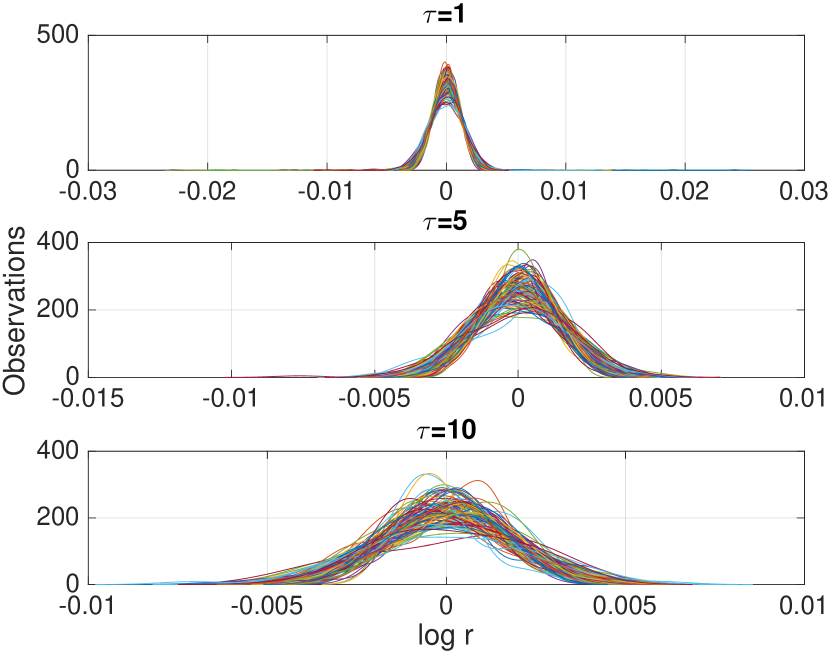
(a) Low-frequency

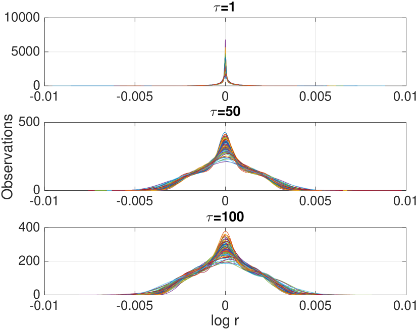
(b) High-frequency

Figure 1: Kernel estimator of the density of log-return for 100 simulations

Note: $\tau$ represents the time scale, days for low-frequency data and transaction events for high-frequency data.

Figures 2(a) and 2(b) show how kurtosis decreases to values below 3 as the time scale increases, a sign of aggregational gaussianity.

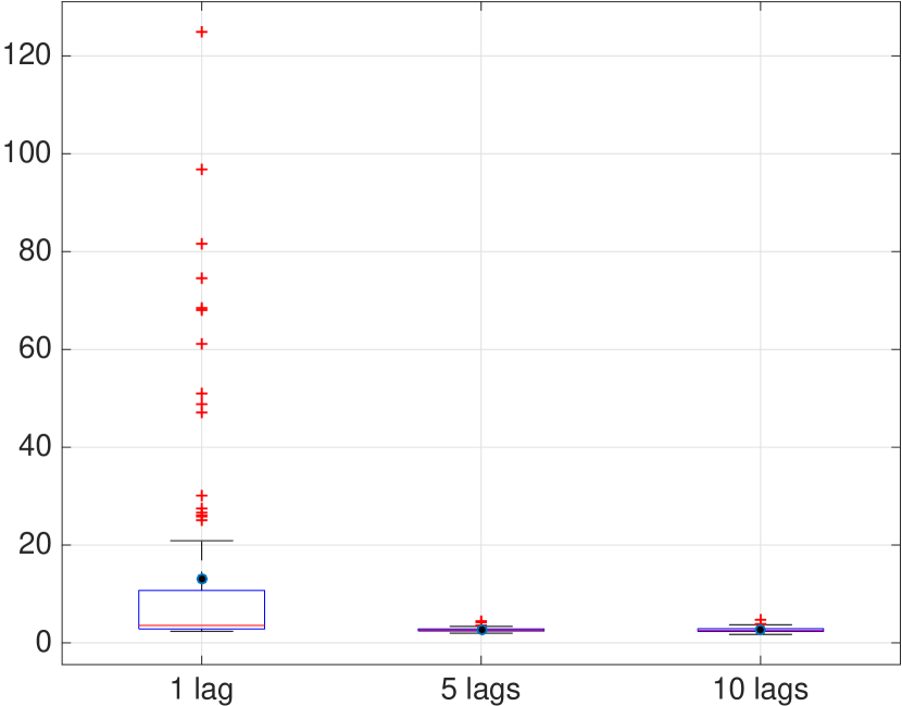
(a) Low-frequency

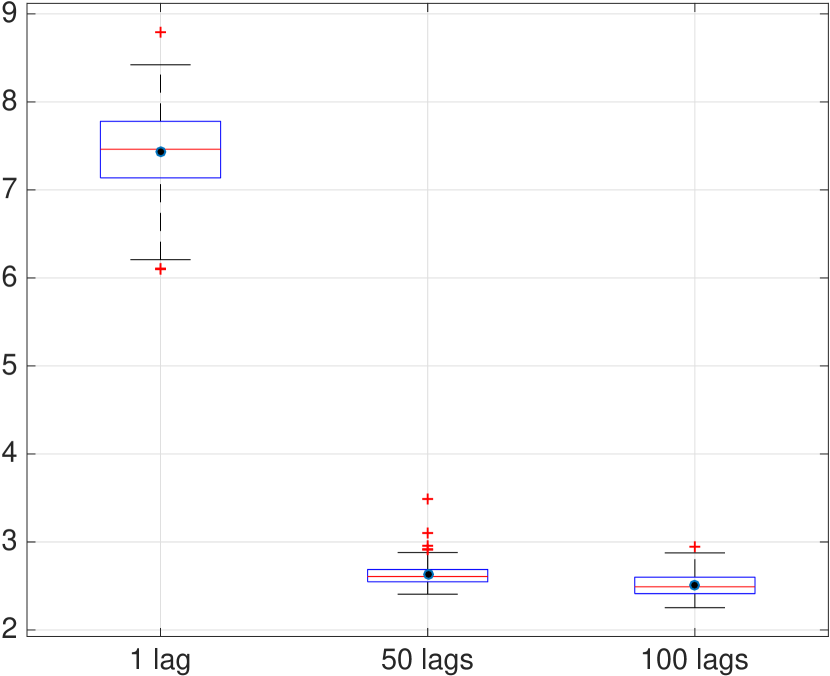
(b) High-frequency

Figure 2: Kurtosis of log-return over 100 simulations

4.1.3 Bubbles and Crashes

We use low-frequency data to investigate the occurence of bubbles and crashes as the fundamental price is a concept applied to low-frequency only. Figure 3(b) confirms the existence of significant positive correlation in lag 0 between asset returns and the relative size of the bubble, as suggested by the empirical evidence (v. 3.1.3).

In cross-correlation confidence bounds are calculated as $\frac{[-numSTD;numSTD]}{\sqrt{N}}$, where $numSTD$ is the number of standard deviations for the sample cross-correlation estimation error assuming variables are uncorrelated, and $N$ is the length of the time-series. We use $numSTD=2$ which corresponds to approximately 95 percent confidence bounds and plots estimation error bounds 2 standard deviations away from 0. We use these calculations in all cross-correlations published.

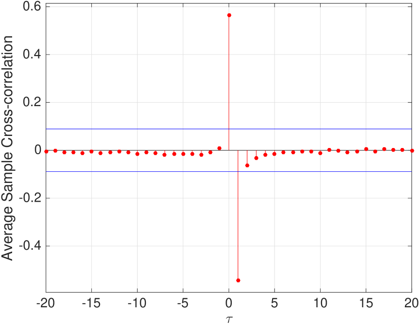
(a) Average cross-correlation

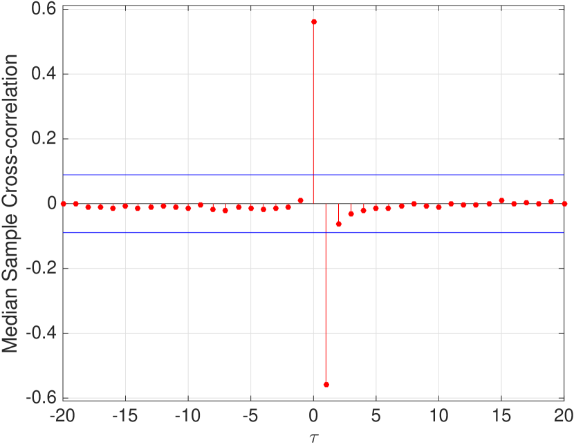
(b) Median cross-correlation

Figure 3: Cross-correlation between bubbles and log-return over 100 simulations

Note: The blue horizontal lines represent the approximate upper and lower confidence bounds $[-0.0892;0.0892]$, assuming bubbles and log-return are uncorrelated.

However the correlation is negative and significant for $\tau=1$, which may suggest the correction of the bubble towards the fundamental price immediately after the positive bubble in $\tau=0$. This may indicate that when the relative size of a bubble and log-return are positively correlated due to a transaction price greater than the fundamental price, as in $\tau=0$, there is a market correction in the next period. This correction could be explained by the fundamentalist component of the agents, which brings the price back to the fundamental price after a positive or negative bubble. Also, the non-existence of either leverage or short-selling generates more stable time-series, closer to the fundamental price, and consequently these corrections are more likely.

The fundamental price is known by all agents who use it to form expectations about next period returns, as previously shown in equation 2. Financial institutions not only use the information on past prices but also actual information on the fundamental price, which is not reflected in past prices and helps agents forecast future returns. Therefore, as the positive (negative) bubble size grows, the fundamentalist component in equation 2 integrates this information into returns expectations and subsequently the financial institutions adjust the direction of the orders down (up) towards the fundamental price. Hence, the fundamentalist component of the returns expectation formation works as a mean-reverting and stabilising process.

Figure 4 shows that the mean bubble size in the unregulated treatment is close to 0, either positive or negative. This reflects the stability of the baseline treatment without capital requirements, leverage or short-selling. However, the experimental treatment with leverage exhibits large and positive bubbles. This suggests that these results could be very different if another treatment was used to study the size of bubbles.

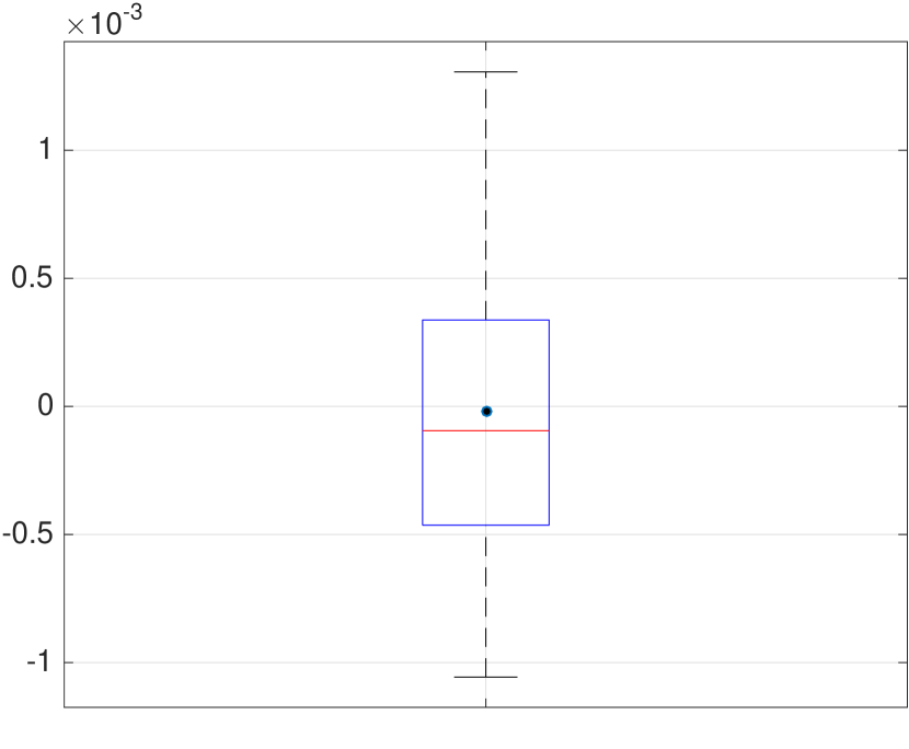
(a) Boxplot

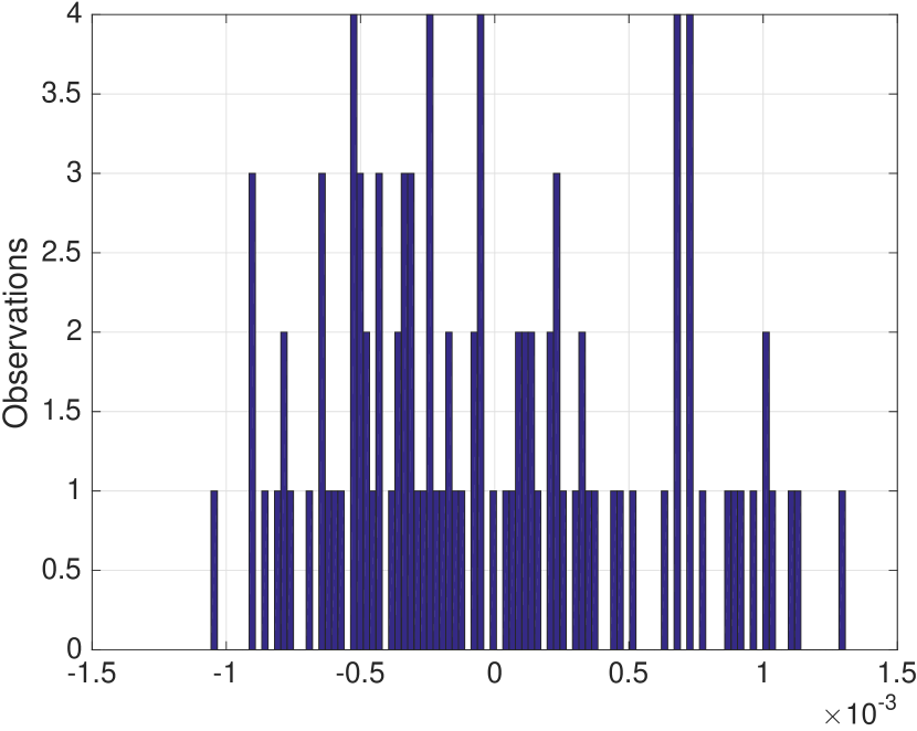
(b) Histogram

Figure 4: Mean size of bubbles over 100 simulations

Contrary to what other studies suggest (e.g. [52]), the existence of bubbles in our model cannot be explained by the misspecification of fundamentals, since the fundamental price is public and known to all agents. Hence, in this case the possible deviation from the fundamental price is due to speculative behaviour originating from chartist and noise trading components.

4.1.4 Heavy Tails of Return Distribution

Figure 5(b) shows that log-return distribution has a heavy-tailed distribution in high-frequency data. In low-frequency data, half of the observations exhibit a kurtosis of 3, which is the kurtosis for normal distributions. Therefore, the higher the frequency of price observations the greater the kurtosis.

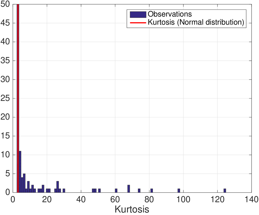
(a) Low-frequency

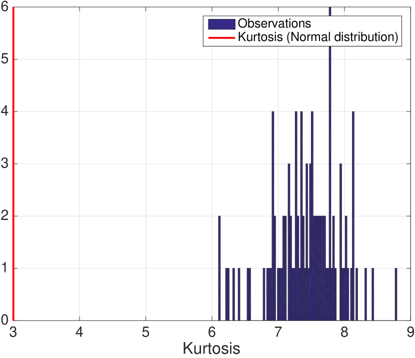
(b) High-frequency

Figure 5: Kurtosis for 100 simulations

Note: The kurtosis is 3 for the standard Normal distribution.

Despite the fact that half of the daily observations exhibit a kurtosis of 3, table 2 shows that the analysis of the mean and median kurtosis for the unregulated treatment indicates a kurtosis greater than 3 [118]. The shape of the distribution is more leptokurtic for mean and median kurtosis in high-frequency data, except for the mean of the low-frequency unregulated treatment. The analysis of kurtosis in treatments with capital requirements reveals the distributions of returns to be more leptokurtic, with particularly high values for high-frequency data.

Table 2: Kurtosis over 100 simulations

	Low-frequency		High-frequency
	Mean	Median	Mean	Median
Unregulated	13.156	3.578	7.426	7.463
VaR	10.505	4.288	255.824	242.133
ES	9.981	4.431	259.851	213.375

Another indicator used to determine the existence of heavy tails is the Hill estimator and the analysis of the tail index. The tail size $k$ was not specified by [57], hence we exhibit results for a bandwidth of tail sizes extending from 1 percent to a maximum of 10 percent of the size of the underlying time-series.

Tables 3 and 4 exhibit the differences between low-frequency and high-frequency data. Table 3 shows high values of the tail index for low-frequency data. The fourth moment – kurtosis – of the distribution does not exist in low-frequency data but only for a tail sample of 10 percent. All other moments exist and are finite. The tail index is smaller for treatments with capital requirements than for the unregulated treatment. These results show greater instability in the VaR and ES treatments relative to the unregulated treatment. The Hill estimator is known to be asymptotically normal and consistent [119, 120, 80]. Low-frequency data sample size is $n=503$, which is not a large sample. As the Hill estimator tends to overestimate the tail exponent of the stable distribution if the sample size is not very large, we analyse the true tail behaviour using larger data sets of high-frequency.

Table 3: Hill estimator for low-frequency returns over 100 simulations

		Tail index
		Mean		Median
	Tail sample	Left	Right	Left	Right
	$1\%$	8.71	8.84	7.46	7.91
	$2.5\%$	6.28	6.25	6.00	6.37
Unregulated	$5\%$	4.82	4.90	4.83	4.83
	$10\%$	3.52	3.71	3.52	3.64
	$1\%$	6.38	7.48	5.13	6.84
	$2.5\%$	5.40	5.73	4.74	5.41
VaR	$5\%$	4.20	4.45	4.00	4.37
	$10\%$	3.16	3.37	3.14	3.43
	$1\%$	7.44	7.19	6.61	5.95
	$2.5\%$	5.74	5.79	5.08	5.09
ES	$5\%$	4.43	4.60	4.34	4.55
	$10\%$	3.27	3.43	3.26	3.45

Table 4 for high-frequency data shows that the fourth moment only exists in the unregulated treatment with a tail size of 1 percent. As in low-frequency data the treatments with capital requirements exhibit smaller tail indices relative to the unregulated treatment, reflecting higher instability. However, the tail index for high-frequency returns is considerable smaller than for low-frequency, which may demonstrate the higher market instability at lower tick sizes or the overestimation of the Hill estimator using low-frequency data.

Table 4: Hill estimator for high-frequency returns over 100 simulations

		Tail index
		Mean		Median
	Tail sample	Left	Right	Left	Right
	$1\%$	5.36	5.40	5.39	5.49
	$2.5\%$	3.85	3.90	3.85	3.89
Unregulated	$5\%$	2.78	2.84	2.77	2.82
	$10\%$	1.82	1.89	1.80	1.88
	$1\%$	2.85	2.93	2.77	2.89
	$2.5\%$	2.81	2.87	2.87	2.93
VaR	$5\%$	2.39	2.40	2.44	2.41
	$10\%$	1.79	1.76	1.77	1.74
	$1\%$	3.36	3.42	3.37	3.43
	$2.5\%$	3.10	3.17	3.16	3.20
ES	$5\%$	2.53	2.56	2.55	2.55
	$10\%$	1.82	1.82	1.80	1.80

4.1.5 Conditional Heavy Tails

Tables 5 (mean) and 6 (median) exhibit results similar to the unconditional heavy tails and confirm the differences between treatments with conditional heavy tails (t or Gaussian). The implementation of financial regulation reduces the tail index and, consequently, increases the occurrence of extreme events.

Table 5: Conditional Hill Estimator over 100 simulations (mean)

		Tail index
		Unconditional		Conditional t		Conditional Gaussian
	Tail sample	Left	Right	Left	Right	Left	Right
	$1\%$	5.36	5.40	4.22	4.22	4.68	4.73
	$2.5\%$	3.85	3.90	3.06	3.06	3.47	3.50
Unregulated	$5\%$	2.78	2.84	2.30	2.33	2.59	2.67
	$10\%$	1.82	1.89	1.67	1.65	1.83	1.94
	$1\%$	2.85	2.93	3.86	2.83	4.13	2.87
	$2.5\%$	2.81	2.87	2.98	2.58	3.25	2.73
VaR	$5\%$	2.39	2.40	2.33	2.15	2.58	2.31
	$10\%$	1.79	1.76	1.76	1.66	1.96	1.80
	$1\%$	3.36	3.42	4.04	3.21	4.26	3.25
	$2.5\%$	3.10	3.17	3.08	2.81	3.28	2.92
ES	$5\%$	2.53	2.56	2.38	2.27	2.55	2.39
	$10\%$	1.82	1.82	1.76	1.72	1.90	1.82

Table 6: Conditional Hill Estimator over 100 simulations (median)

		Tail index
		Unconditional		Conditional t		Conditional Gaussian
	Tail sample	Left	Right	Left	Right	Left	Right
	$1\%$	5.39	5.49	4.22	4.21	4.62	4.67
	$2.5\%$	3.85	3.89	3.05	3.07	3.41	3.46
Unregulated	$5\%$	2.77	2.82	2.28	2.33	2.56	2.64
	$10\%$	1.80	1.88	1.49	1.74	1.81	1.93
	$1\%$	2.77	2.89	3.95	2.84	4.18	2.85
	$2.5\%$	2.87	2.93	2.98	2.58	3.23	2.70
VaR	$5\%$	2.44	2.41	2.30	2.11	2.56	2.25
	$10\%$	1.77	1.74	1.74	1.64	1.97	1.78
	$1\%$	3.37	3.43	4.07	3.21	4.30	3.23
	$2.5\%$	3.16	3.20	3.01	2.74	3.28	2.88
ES	$5\%$	2.55	2.55	2.32	2.18	2.55	2.35
	$10\%$	1.80	1.80	1.74	1.67	1.93	1.81

Table 7 shows that the conditional residual time-series generated from our model still exhibit a leptokurtic distribution either with t or Gaussian white noise.

Table 7: Conditional kurtosis over 100 simulations (high-frequency data)

	Unconditional		Conditional t		Conditional Gaussian
	Mean	Median	Mean	Median	Mean	Median
Unregulated	7.43	7.46	10.19	10.25	8.29	8.47
VaR	255.82	242.13	332.28	248.66	266.38	232.49
ES	259.85	213.38	268.29	218.30	259.85	206.65

The returns are heavy-tailed even when applying a model that compensates for the time varying volatility. We conclude that our model replicates the stylised fact of conditional heavy tales found in empirical data (v. 3.1.5).

4.1.6 Equity Premium Puzzle

The equity premium documented in [65] is for very long investment horizons and it has varied considerably and counter-cyclically over time. Table 8 shows the equity premium in our baseline treatment. A possible explanation for the negative premium observed in our model is the stability of the baseline treatment and mean realised returns of approximately zero.

Table 8: Equity Premium Puzzle over 100 simulations (unregulated)

Annual Mean Return		Equity Premium
Realised	Risk-free Asset	Realised
$2.8\times 10^{-5}$	0.0457	-0.0457 pps

• Note: The annual mean return is calculated using the mean of the realised returns over 100 simulations. The returns of the risk-free asset are fixed.

A possible explanation for the small realised returns and, consequently, the negative equity premium observed, is the mean-variance portfolio optimisation used by the financial institutions. Financial institutions are risk-averse however loss aversion, usually identified as a possible explanation for this stylised fact [121], is not considered in this particular experiment. [117] argued that the equity premium puzzle is one of the stylised facts about stock returns that is difficult to explain in conventional models. [121] show that loss aversion might explain the equity premium puzzle .

4.1.7 Excess Volatility

Table 9 confirms that annual volatility of the market log-return exceeds the annual volatility of the fundamental log-return in all treatments.

In the absence of financial regulations volatility enters the model either through the fundamental price or through traders’ behaviour. As the annual mean volatility of the fundamental price is the same for all treatments and the agents’ initial conditions are the same in all treatments, the only source of volatility that differs between treatments is the implementation of regulation.

Table 9: Excess volatility of log-return over 100 simulations

	Annual Mean Volatility
	Market	Fundamental
Unregulated	0.0197	0.006
VaR	0.0236	0.006
ES	0.0216	0.006

• Note: The volatility is calculated using the standard deviation of the log-return for each of the treatments: Unregulated, VaR and ES.

4.1.8 Gain/Loss Asymmetry

Table 10 shows our analysis of the investment horizon distribution $p(\tau_{\rho})$ for a return level of $\rho=0.25$ percent. The most likely horizon, which we call the optimal investment horizon, is greater for gains than for losses, and accords with the empirical evidence. These waiting times are longer in the unregulated treatment as it shows less volatility. The more volatile VaR and ES treatments exhibit a smaller time span needed to generate a fluctuation or a movement in the price of size $\rho=0.25$ percent.

Table 10: Optimal Investment Horizon over 100 simulations

	Gains			Losses
	Mean	Median	Std	Mean	Median	Std
Unregulated	8.28	6	(6.78)	6.5	5.5	(5.31)
VaR	4.22	2	(5.02)	2.98	2	(2.43)
ES	5.02	2	(6.97)	3.73	3	(2.97)

• Note: We analyse the daily closure for all the 100 simulations for each of the treatments – unregulated, VaR and ES. The optimal investment horizons over 100 simulations were computed by generating 100 independent realisations of our model across 504 days, computing the daily return for each realisation, and then calculating the necessary time horizon to reach a return level of $\rho=0.25$ percent. The values in parenthesis are standard deviations.

4.1.9 Leverage Effect

Figure 6 shows that the unregulated treatment does not generate leverage effects in low-frequency data.

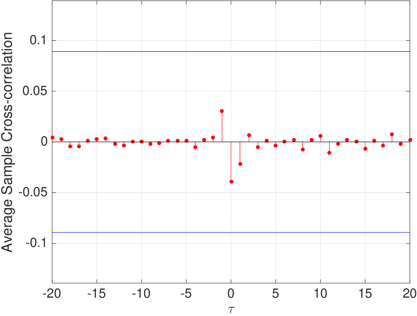
(a) Average Returns

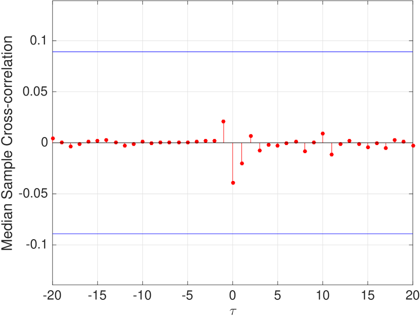
(b) Median Returns

Figure 6: Leverage effects of low-frequency log-return over 100 simulations

Note: The blue horizontal lines represent the approximate upper and lower confidence bounds $[-0.0892;0.0892]$, assuming log-return and volatility are uncorrelated.

Figure 7 shows that in high-frequency data the leverage effect is negative and significant for $\tau=0$. The observed negative leverage implies that volatility and returns are negatively correlated: price drops increase volatility of an asset, this is the so-called leverage effect.

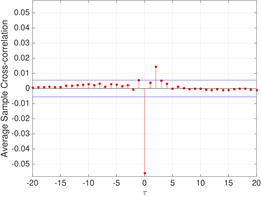
(a) Average Returns

(b) Median Returns

Figure 7: Leverage effects of high-frequency over 100 simulations

Note: The blue horizontal lines represent the mean of approximate upper and lower confidence bounds over 100 simulations $[-0.0063;0.0063]$, assuming log-return and volatility are uncorrelated.

According to [73] the leverage effect is much more pronounced for indices than single stocks. For both stocks and stock indices, the volatility-return correlation is short ranged, with, however, a shorter decay time for stock indices than for individual stocks, and the amplitude of the correlation is much stronger for indices than for individual stocks.

4.1.10 Linear Autocorrelation

As mentioned in section 3.1.10, [77] demonstrates that the first-order autocorrelations of daily returns are positive for twenty-two out of thirty stocks of the DJIA, which means that this dependence is negative for eight stocks. Figure 8(b) indicates that daily returns in the unregulated treatment exhibit first-order negative autocorrelation.

The estimated standard error for the autocorrelation at lag $k>q$ is

$$SE(r_{k})=\sqrt{\frac{1}{T}(1+2\sum^{q}_{j=1}{r_{j}^{2}})}.$$

Confidence bounds are calculated as

$$SE(r_{k})\times[-numSTD;numSTD]$$

where $numSTD$ is the number of standard deviations for the sample autocorrelation function estimation error assuming the theoretical autocorrelation function is 0 beyond lag 0. Since we assume that the moving average order that specifies the number of lags beyond which the theoretical autocorrelation function is effectively 0 equals 0, confidence bounds can be expressed as $\frac{[-numSTD;numSTD]}{\sqrt{T}}$. $T$ is the length of the time-series. We use $numSTD=2$ which corresponds to approximately 95 percent confidence bounds. These calculations are used in all autocorrelations published.

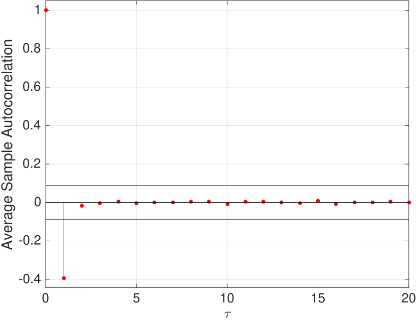
(a) Average

(b) Median

Figure 8: Autocorrelation in low-frequency log-return over 100 simulations

Note: The blue horizontal lines represent the approximate confidence bounds $[-0.0892;0.0892]$ of the autocorrelation function assuming the time serie is a moving average process.

[77] further demonstrates that the preponderance of positive or negative signs in the coefficients for the daily data are partly determined by factors peculiar to that asset or industry. However, this author concludes that the actual direction of the “dependence” varies from study to study. We believe that the lag 1 negative autocorrelation observed in our experimental treatment might be caused by the dominance of agents’ fundamentalist component that brings the price back to the fundamentalist price.

Figure 9 shows that intraday returns from traded assets are almost uncorrelated, with any important dependence usually restricted to a negative correlation between consecutive returns in very small intraday time scales [39, 5]. This first-order negative autocorrelation is traditionally attributed to microstructure effects, as the bid-ask bounce, due to the fact that there is often a spread between the price paid by buyer and seller initiated trades and the transaction prices may take place either close to the ask or closer to the bid price, which tend to bounce between these two limits [83].

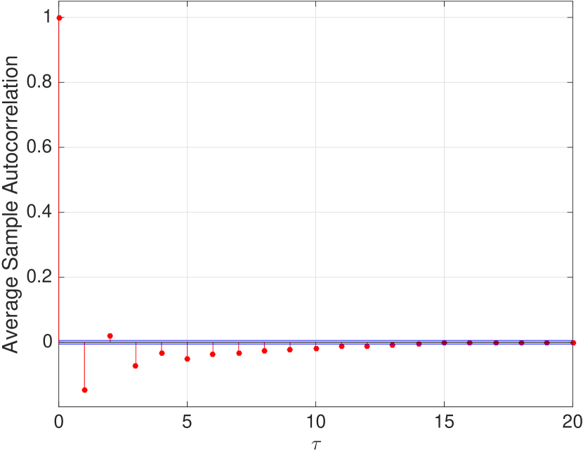
(a) Average Autocorrelation

(b) Median Autocorrelation

Figure 9: Absence of autocorrelation in high-frequency log-return over 100 simulations

Note: The blue horizontal lines represent the approximate confidence bounds $[-0.0063;0.0063]$ of the autocorrelation function assuming the time serie is a moving average process.

4.1.11 Long Memory

Figure 10(b) shows that in low-frequency time-series there is a short term positive dependence among absolute log-return [39], marginally significant only in the first period.

(a) Average

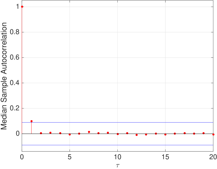
(b) Median

Figure 10: Long memory in low-frequency log-return over 100 simulations

Note: The blue horizontal lines represent the approximate confidence bounds $[-0.0892;0.0892]$ of the autocorrelation function assuming the time-series is a moving average process.

However, figure 11(b) shows that in high-frequency time-series the autocorrelation function of absolute log-return decays slowly and this is sometimes interpreted as a sign of long-range dependence.

(a) Average

(b) Median

Figure 11: Long Memory in high-frequency log-return over 100 simulations

Note: The blue horizontal lines represent the approximate confidence bounds $[-0.0063;0.0063]$ of the autocorrelation function assuming the time-series is a moving average process.

[95] observe that long-range volatility correlations arise from trading activity, which we cover in sections 4.4–16.

4.1.12 Power Law Behaviour of Returns

Table 11 shows the results of all the steps described in sections 25–3.1.12. If the calculated p-value is smaller than 0.05 then we rule out the power-law hypothesis. Conversely, the hypothesis is a plausible one for the data in question. Normally low values of $p$ are considered to be good, since they indicate that the null hypothesis is unlikely to be correct. In [80], by contrast, the p-value is used as a measure of the hypothesis we are trying to verify, and hence high values do not reject the power-law hypothesis. We use this analysis when investigating the existence of power laws distributions.

Table 11: Power law of returns over 100 simulations

	Mean	Median	Standard Deviation
$\hat{\zeta_{r}}$	6.37	5.75	(2.42)
$\hat{x}_{min}$	0.0019	0.0018	($3.95\times 10^{-4}$)
p-value	0.32	0.18	(0.32)
Uncertainty $\hat{\zeta_{r}}$	1.91	1.58	(1.18)
Uncertainty $\hat{x}_{min}$	$3.11\times 10^{-4}$	$2.91\times 10^{-4}$	$9.27\times 10^{-5}$

• Note: In the unregulated treatment with low-frequency data, 76 out of 100 simulations have a p-value greater than 0.05, and therefore consistent with the hypothesis that $x$ is drawn from a distribution of the form of equation 24.

Contrary to what is found in employing the Hill estimator, the applicability of the power law estimators used by [80] to smaller data sets is not considered to be a problem. [80] suggest that a sample of $n=50$ is a reasonable rule of thumb for extracting reliable parameter estimates. Our low-frequency data sets are $n=503$, and therefore can be considered as being sufficiently large to estimate reliable scaling parameters.

We conclude that 76 out of 100 returns distributions follow a power-law distribution and that the scaling parameter of the power-law behaviour of returns is greater than the typical inverse cubic, as is usual on longer time scales [122]. Hence, our experimental treatment confirms the scaling behaviour for the majority of simulations, despite the return distribution scale lying outside the stable Lévy-regime. [122] states that a more Gaussian exponent is common in longer time scales, and [123] refers the case of the DAX as another example of a power law behaviour outside the Lévy-stable range.

[124] and [95] conclude that the number of trades, as covered in sections 4.4–16, cannot alone explain the value $\zeta_{r}\approx 3$ and suggest that the pronounced tails of the distribution of returns are possibly due to local variance.

4.1.13 Power Law Behaviour of Volatility

Table 12 shows the regression fits of low-frequency volatility for an averaging window T=5 days with $\Delta{t}=1$ day. According to [82], the larger the choice of time interval T, the more accurate is the volatility estimation, but a large value for T also implies poor resolution in time. Hence we opted for a time interval of 5.

Table 12: Power law of volatility over 100 simulations

	Mean	Median	Standard Deviation
$\hat{\zeta_{\sigma}}$	6.96	5.93	(4.06)
$\hat{x}_{min}$	0.0011	0.0011	($2.14\times 10^{-4}$)
p-value	0.52	0.54	(0.32)
Uncertainty $\hat{\zeta_{\sigma}}$	2.60	1.91	(1.90)
Uncertainty $\hat{x}_{min}$	$1.63\times 10^{-4}$	$1.6\times 10^{-4}$	($5.07\times 10^{-5}$)

• Note: In the low-frequency unregulated treatment, 92 out of 100 simulations have a p-value greater than 0.05, and are therefore consistent with the hypothesis that $x$ is drawn from a distribution of the form of equation 28.

From the estimates we find that the cumulative distribution of low-frequency volatility is consistent with a power law asymptotic behaviour (as in equation 28) in 92 percent of simulations. The results reveal that the estimates of $\zeta_{\sigma}$ for T=5 days with $\Delta t=1$ day lie outside the stable Lévy range of $0<\zeta_{\sigma}<2$.

4.1.14 Volatility Clustering

Figure 12 shows that the magnitude of this effect is close to zero in low-frequency returns, except for the first-order correlation, which is not significant across all simulations.

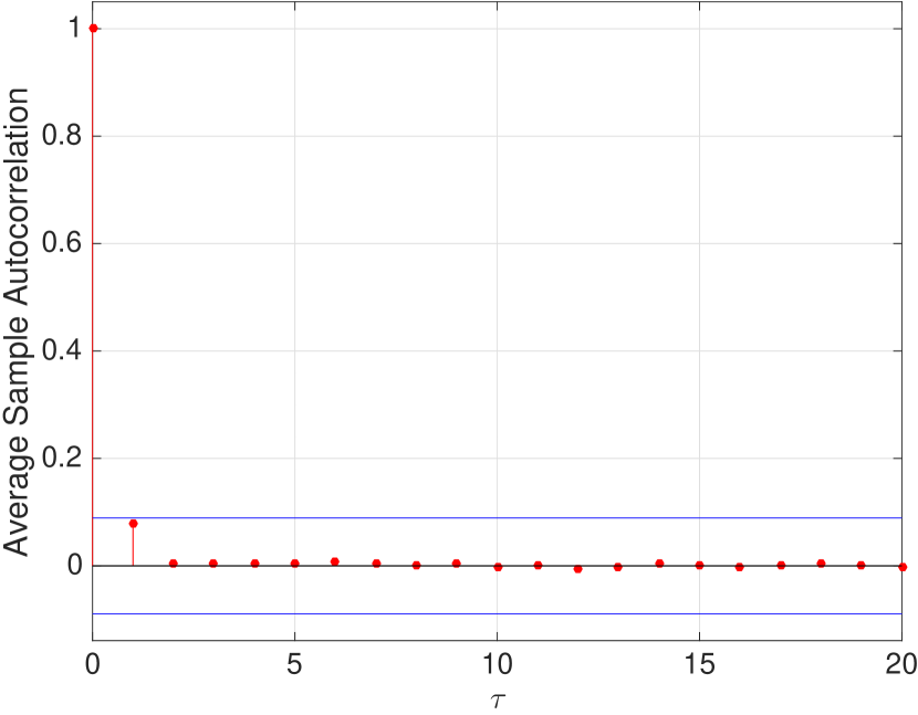
(a) Average Autocorrelation

(b) Median Autocorrelation

Figure 12: Volatility clustering in daily squared returns over 100 simulations

Note: The blue horizontal lines represent the approximate confidence bounds $[-0.0892;0.0892]$ of the autocorrelation function assuming the time serie is a moving average process.

Figure 13 shows serial correlation effects in high-frequency returns, prolonged and higher than in low-frequency returns. The autocorrelation function of volatility decreases slowly to zero and is statistically significant for long time periods. The positive results obtained for the autocorrelation function of the squared returns and their slow decay are verified in empirical financial data and are often mentioned as a “quantitative manifestation” of volatility clustering [56].

(a) Average Autocorrelation

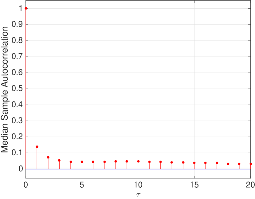
(b) Median Autocorrelation

Figure 13: Volatility clustering in high-frequency squared returns over 100 simulations

Note: The blue horizontal lines represent the approximate confidence bounds $[-0.0063;0.0063]$ of the autocorrelation function assuming the time serie is a moving average process.

4.1.15 Volatility Volume Correlations

Figure 14 exhibits cross-correlation between volatility and volume for low-frequency data that is not statistically significant.

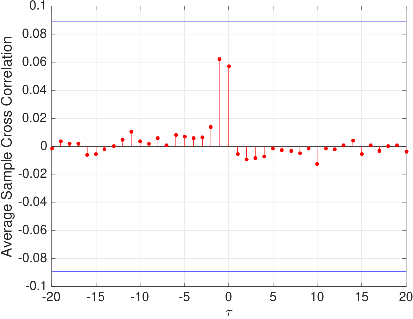
(a) Average cross-correlation

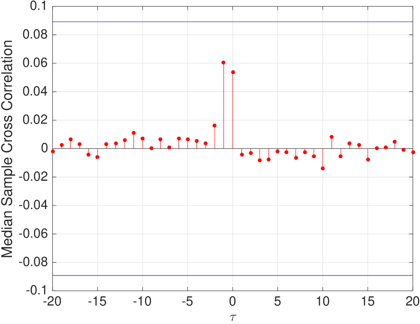
(b) Median cross-correlation

Figure 14: Cross-correlation between volatility and trading volume in low-frequency data over 100 simulations

Note: The blue horizontal lines represent the approximate upper and lower confidence bounds $[-0.0892;0.0892]$, assuming volatility and trading volume are uncorrelated.

However, figure 15 shows that the cross-correlation between volatility and volume for high-frequency data is positive and both volatility and volume show the same type of “long memory” behaviour [85, 56]. The cross-correlation function of the high-frequency data was analysed by aggregating and averaging the data over intervals of 30 ticks.

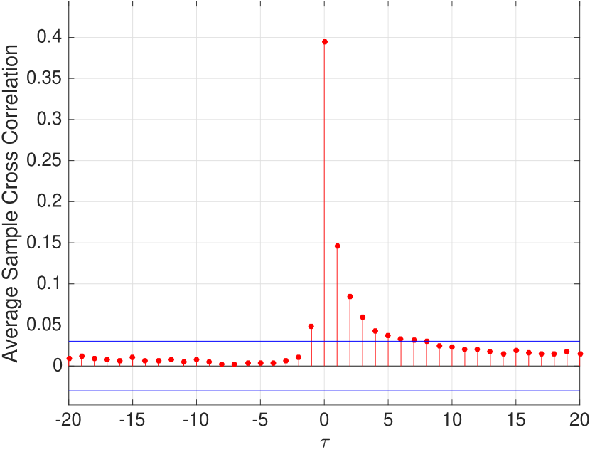
(a) Average cross-correlation

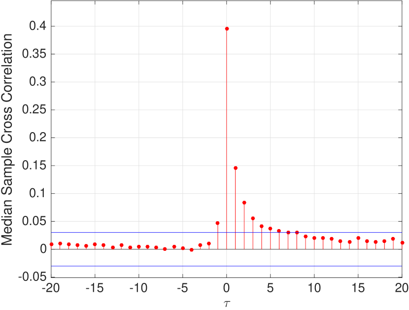
(b) Median cross-correlation

Figure 15: Cross-correlation between volatility and trading volume in high-frequency data over 100 simulations

Note: The blue horizontal lines represent the mean of approximate upper and lower confidence bounds over 100 simulations $[-0.0345;0.0345]$, assuming volatility and trading volume are uncorrelated.

We also analyse the frequency of trades to identify any relationship between volatility and the number of trades. Figure 16 shows that there is no significant cross-correlation for low-frequency data.

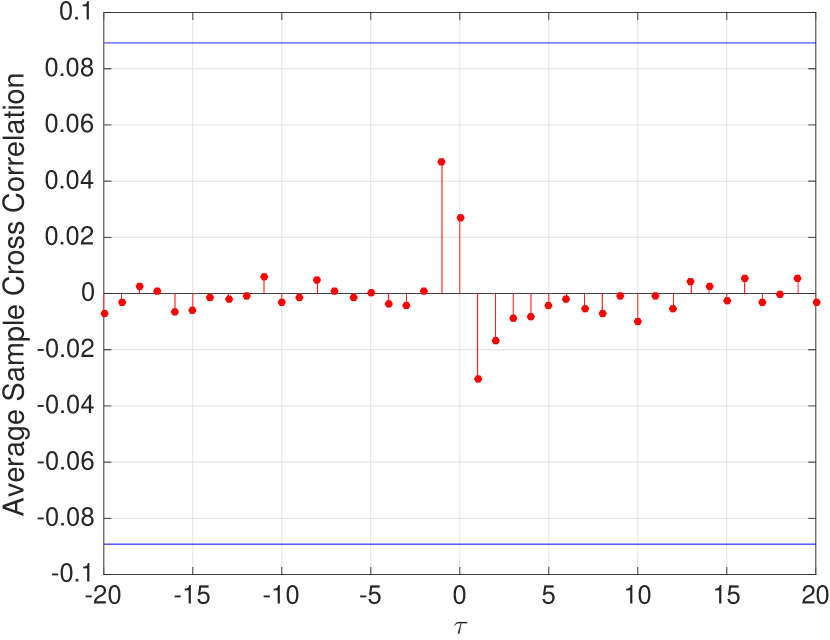
(a) Average cross-correlation

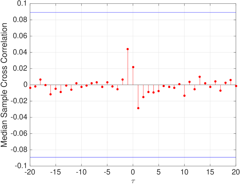
(b) Median cross-correlation

Figure 16: Cross-correlation between volatility and number of trades in low-frequency data over 100 simulations

Note: The blue horizontal lines represent the approximate upper and lower confidence bounds $[-0.0892;0.0892]$, assuming volatility and number of trades are uncorrelated.

In Figure 17 we observe that volatility and the number of trades only exhibit significant and positive correlation for current number of trades in high-frequency data and is only marginally significant for past trades in lag -1, as observed in [71]. [56] observes that the heterogeneity in agents’ time horizons, as in our model, may lead to volatility-volume relationships similar to those of actual markets.

(a) Average cross-correlation

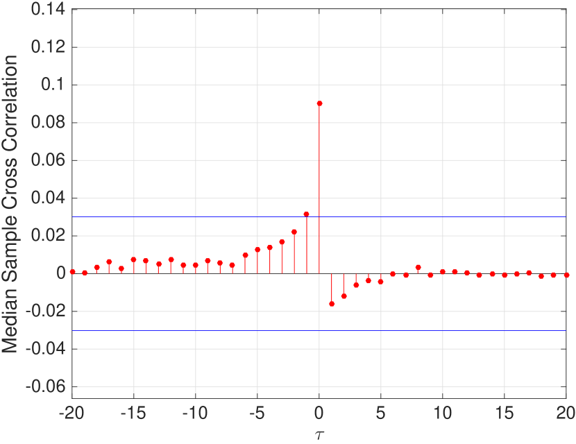
(b) Median cross-correlation

Figure 17: Cross-correlation between volatility and number of trades in high-frequency data over 100 simulations

Note: The blue horizontal lines represent the mean of approximate upper and lower confidence bounds over 100 simulations $[-0.0345;0.0345]$, assuming volatility and number of trades are uncorrelated.

4.1.16 Unit Roots

Table 13 shows the results from the Phillips-Perron Unit Root Tests. We can conclude that the time-series of log-return are stationary for low- and high-frequency data.

Table 13: Phillips-Perron Unit Root Tests

		Phillips-Perron
		Test statistics	p-value	Critical value
Unregulated	LF	[-40.31; -23.24]	0.001	-1.9411
	HF	[-422.04; -288.16]	0.001	-1.9416
VaR	LF	[-39.37; -25.97]	0.001	-1.9411
	HF	[-727.14; -381.31]	0.001	-1.9416
ES	LF	[-38.59; -27.43]	0.001	-1.9411
	HF	[-653.47; -329.11]	0.001	-1.9416

• Note: ADF tests present similar results. All unit roots tests indicate rejection of the unit-root null in favor of the alternative model, then stationarity. Significance level for the hypothesis tests is 0.05. Intervals represent minimum and maximum values of the statistical test. The number of lagged difference terms is 0. Model variant is autoregressive. Test statistic is standard t statistic using ordinary least squares estimates of the coefficients in the alternative model, and p-values are left-tail probabilities.

In Table 14 we apply the KPSS test which shows that all the simulated time-series of returns are stationary. These results are consistent with the findings that usually prices are not stationary but returns, the differences, are [89, 90].

Table 14: Stationarity Tests

		KPSS
		Test statistics	p-value	Critical value
Unregulated	LF	[0.002; 0.077]	0.1	0.1460
	HF	[$6.54\times 10^{15};$$6.9\times 10^{-5}$]	0.1	0.1460
VaR	LF	$[0.0027;0.0787]$	0.1	0.1460
	HF	[$2.62\times 10^{-4}$; $3.08\times 10^{-5}$]	0.1	0.1460
ES	LF	$[0.0027;0.0834]$	0.1	0.1460
	HF	[$3.4\times 10^{-5}$; $3.53\times 10^{-4}$]	0.1	0.1460

• Notes: All treatments fail to reject the null hypothesis that returns are stationary. Significance level for the hypothesis tests is 0.05. Intervals represent minimum and maximum values of the statistical test. The number of autocovariance lags to include in the Newey-West estimator of the long-run variance is 0. The deterministic trend term $\delta t$ is included in the model. KPSS tests compute test statistics using an ordinary least squares (OLS) regression. Critical values are for right-tail probabilities.

4.2 Trading Volume

As mentioned in sections 3.2–3.2.2, there is no consensus about the distribution of trading volume being Lévy-stable [33]. The results from our model show scaling parameters falling outside the Lévy-stable interval.

4.2.1 Power Law Behaviour of Trading Volume

Table 15 exhibits extremely high scaling parameters, which indicate the existence of a power law behaviour outside the Lévy-stable interval. Nevertheless, our results show that 76 out of 100 simulations exhibit p-values consistent with the existence of a power law distribution.

Table 15: Power law of trading volume over 100 simulations

	Mean	Median	Standard Deviation
$\hat{\zeta_{V}}$	17.50	16.86	(4.32)
$\hat{x}_{min}$	11763	11801	(740.67)
p-value	0.976	0.242	(0.323)
Uncertainty $\hat{\zeta_{V}}$	4.17	3.90	(1.60)
Uncertainty $\hat{x}_{min}$	604.81	575.44	(186.04)

• Note: In the low-frequency unregulated treatment, 76 out of 100 simulations have a p-value greater than 0.05, and therefore are consistent with the hypothesis that $x$ is drawn from a distribution of the form of equation 36.

4.2.2 Long Memory of Volume

Figure 18 shows that low-frequency trading volume data does not exhibit significant long-memory.

(a) Average autocorrelation

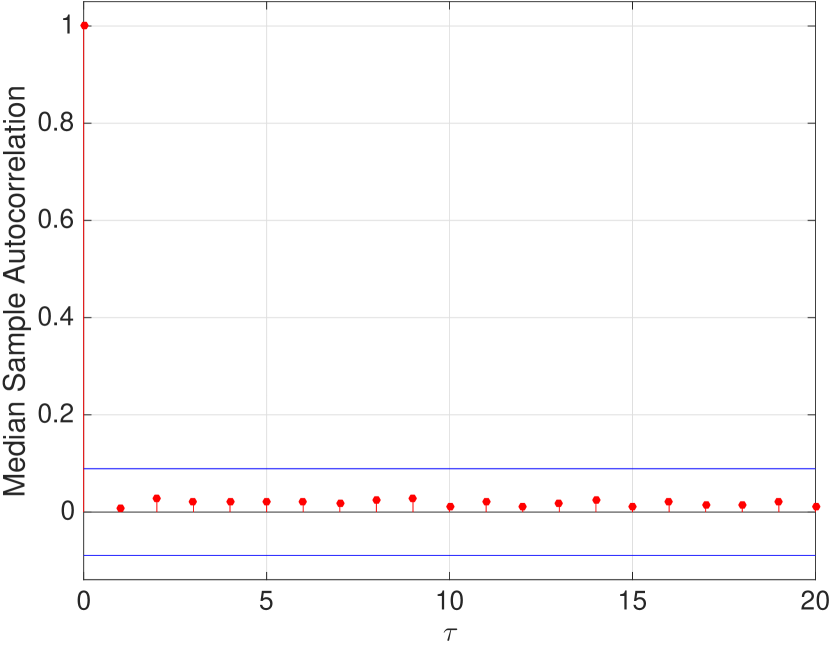
(b) Median autocorrelation

Figure 18: Autocorrelation of trading volume in low-frequency data over 100 simulations

Note: The blue horizontal lines represent the approximate confidence bounds $[-0.0891;0.0891]$ of the autocorrelation function assuming the time serie is a moving average process.

However, Figure 19 exhibits significant long memory across many transactions for high-frequency data, as confirmed by the empirical evidence, e.g. [83]. These results indicate the existence of clustering of volume.

(a) Average autocorrelation

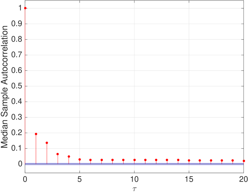
(b) Median autocorrelation

Figure 19: Autocorrelation of trading volume in high-frequency data over 100 simulations

Note: The blue horizontal lines represent the approximate confidence bounds $[-0.0053;0.0053]$ of the autocorrelation function assuming the time serie is a moving average process.

4.3 Trading Duration

In our baseline treatment across 100 simulations, the minimum time observed between events is 1 tick and the maximum duration is 184 ticks. The average duration between successive events is 10.24 ticks with a standard deviation of 9.70 ticks.

[88] observes that longer durations are associated with lower volatilities as predicted by the Easley and O’Hara model [103], and is discussed in sections 4.1.15–16.

4.3.1 Clustering of Trade Duration

Figure 20 shows the existence of positive autocorrelation of squared trading duration starting at low values and exhibiting slow decay of the autocorrelation function only in treatments with risk-based capital requirements. The baseline treatment does not show any significant autocorrelation of trading duration. [102] observe that these autocorrelations indicate clustering of durations, as identified in empirical data.

(a) Baseline (average)

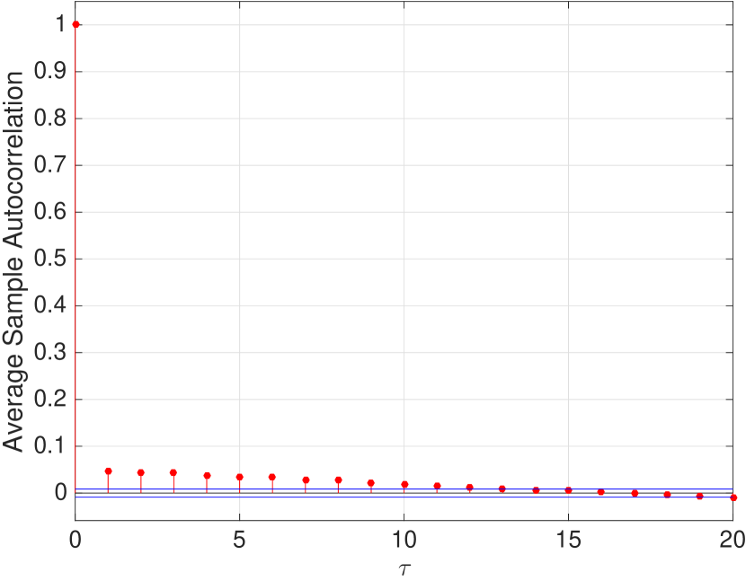
(b) VaR (average)

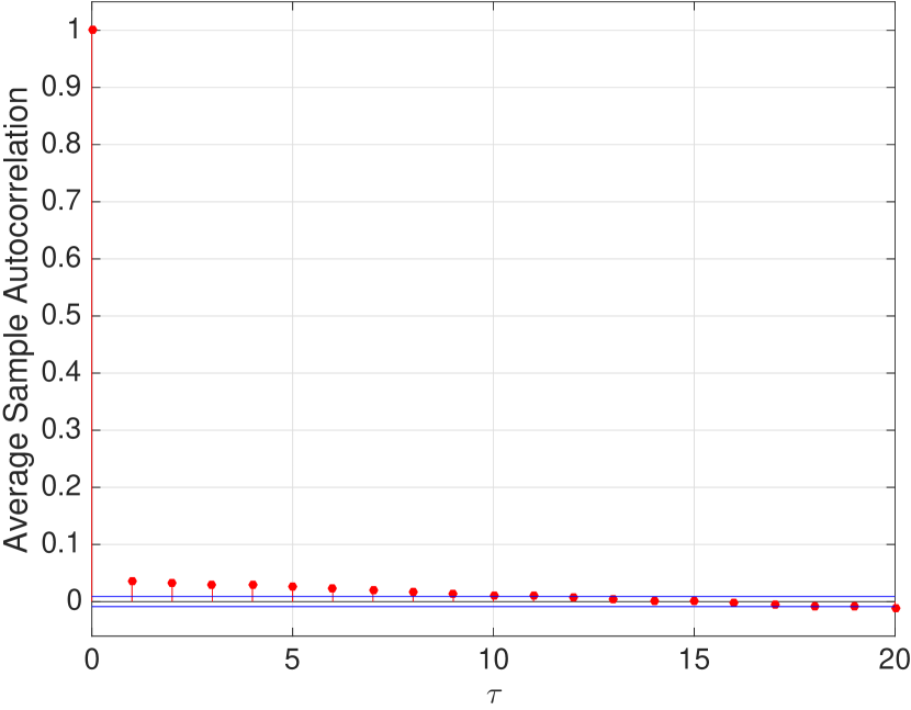
(c) ES (average)

(d) Baseline (median)

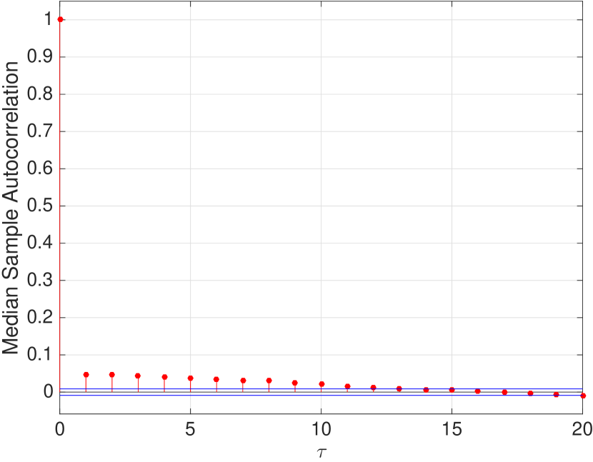
(e) VaR (median)

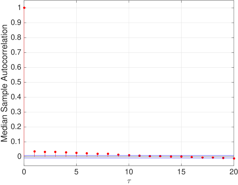
(f) ES (median)

Figure 20: Autocorrelation of squared trading duration in high-frequency data over 100 simulations

Note: The blue horizontal lines represent the average confidence bounds for, respectively, baseline, VaR and ES treatments ($[-0.0126;0.0126]$, $[-0.0104;0.0104]$, $[-0.011;0.011]$) of the autocorrelation function assuming the time-series is a moving average process.

4.3.2 Long Memory of Trade Duration

As for clustering of trade durations, Figure 21 shows the existence of positive autocorrelations of trading duration starting at low values and exhibiting slow decay of the autocorrelation function, but only for treatments with risk-based capital requirements.

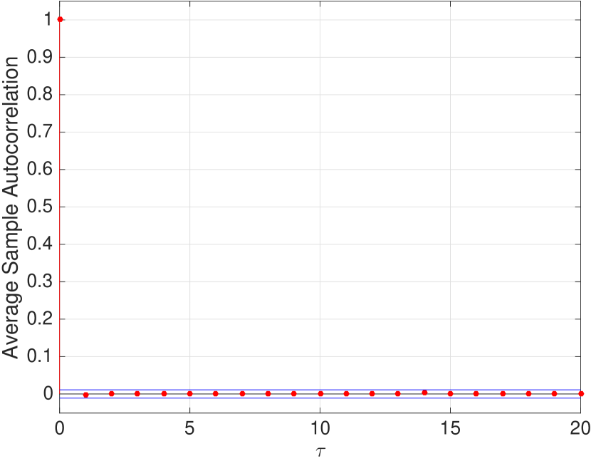
(a) Baseline (average)

(b) VaR (average)

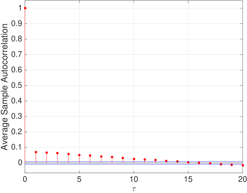
(c) ES (average)

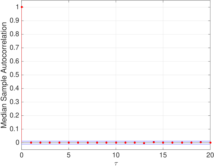
(d) Baseline (median)

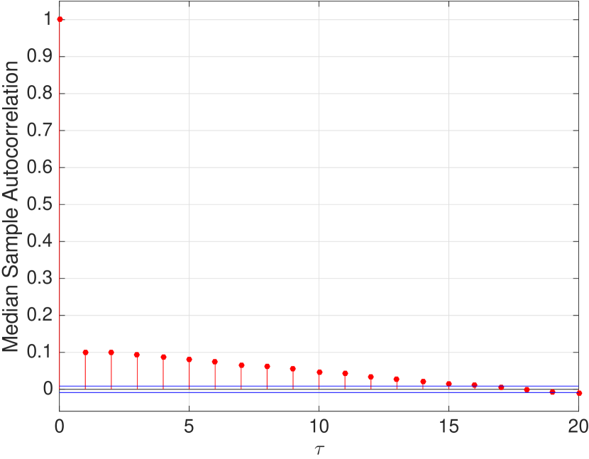
(e) VaR (median)

(f) ES (median)

Figure 21: Autocorrelation of trading duration in high-frequency data over 100 simulations

Note: The blue horizontal lines represent the average confidence bounds ($[-0.0126;0.0126]$, $[-0.0104;0.0104]$, $[-0.011;0.011]$) of the autocorrelation function assuming the time-series is a moving average process.

4.3.3 Overdispersion

Figure 22 shows that the mean of trade durations in treatments with risk-based capital requirements are characterised by overdispersion. The mean of ratio of standard deviation to mean of the duration series is greater than one in VaR (1.038) and ES (1.010) treatments, while the baseline treatments both reveal the same level of underdispersion (0.954).

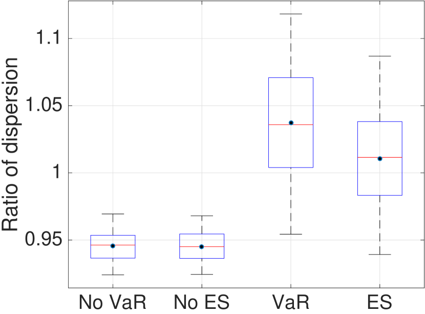
Figure 22: Boxplot of overdispersation of trade durations

We conclude from these results that the stylised facts of trading duration are replicated by our model, but only in treatments with risk-based capital requirements.

4.4 Transaction Size

In this section we investigate if distributions of trading volume are consistent with a Lévy-stable distribution.

4.4.1 Power Law Behaviour of Trades

Table 16 exhibits a different behaviour relative to the previous analysed power laws.

Table 16: Power law of number of trades over 100 simulations

	Mean	Median	Standard Deviation
$\hat{\zeta_{N}}$	3.9	3.9	(0.0)
$\hat{x}_{min}$	227.04	226	(34.08)
p-value	0.0	0.0	(0.0)
Uncertainty $\hat{\zeta_{N}}$	0.0	0.0	(0.0)
Uncertainty $\hat{x}_{min}$	4.10	3.94	(1.08)

• Note: In the low-frequency unregulated treatment, all the simulations have a p-value of 0, which rules out the hypothesis that $x$ is drawn from a distribution of the form of equation 39.

As in [95], we find a mean value $\zeta_{N}=3.9$, which is greater than 2 and therefore outside the Lévy-stable distribution. The fact that all p-values are 0 confirms the evidence in [33] supporting the existence of a non-invariant distribution.

4.5 Bid-ask spread

4.5.1 Spread Correlated with Price Change

The existence of bid-ask spread, although small in magnitude, has several important consequences in time-series properties of asset returns. The bid-ask spread introduces a negative lag 1 serial correlation in the series of observed price changes, as observed in figure 9. This serial correlation in an asset return is referred to as the bid-ask bounce in the finance literature [109]. The same result was also reported in [125] where the authors computed serial correlations of price changes to test for the bid-ask spread effect, which produced a negative average first-order serial correlation meaningfully different from zero.

4.5.2 Thinness and Large Spread

We calculate the bid-ask spread as in equation 40 and investigate the impact of market thinness in both the bid and ask sides of the order-book. In figure 23 we confirm the statistically significant negative correlation between spread and bid volume. However, there is no significant dependence between spread and ask volume.

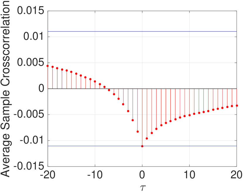
(a) Ask

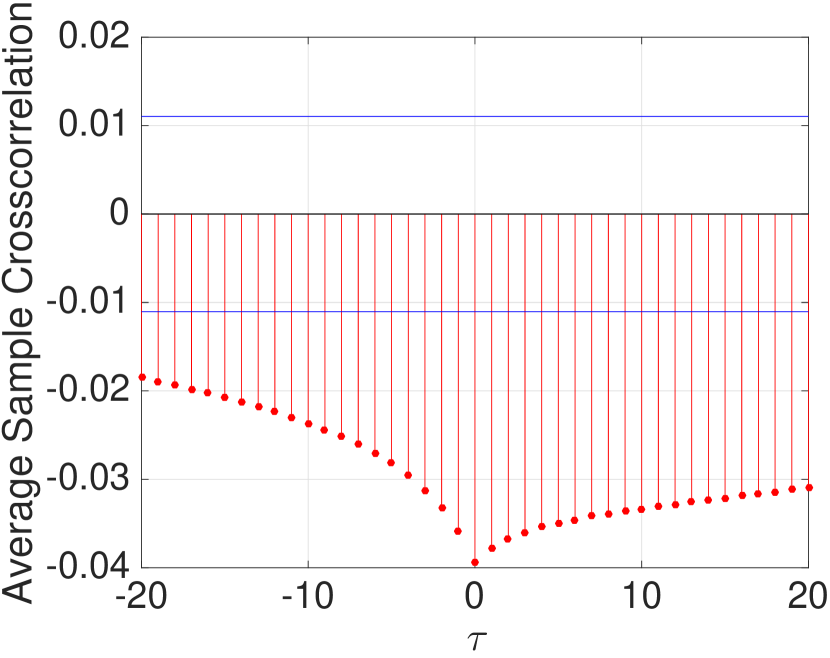
(b) Bid

Figure 23: Cross-correlation between spread and volume in high-frequency data over 100 simulations

Note: The blue horizontal lines represent the mean of approximate upper and lower confidence bounds over 100 simulations ($[-0.0126,0.0126]$), assuming spread and volume are uncorrelated.

5 Conclusion

In this paper we demonstrate that our model is able to robustly and consistently replicate most of the well-known stylised facts of financial time-series data, either with the simplest baseline treatment or treatments with risk-based capital requirements. To the best of our knowledge, this is the first agent-based model which is able to replicate a vast number of stylised facts of financial time-series of returns, trading volume, trading duration, transaction size and bid-ask spread. The ability of our agent-based model to correctly reproduce statistical properties of financial time-series, including the qualitative properties of financial time-series (e.g. heavy tails), their correct quantitative properties (e.g. tail exponent or moments of distribution), and the distribution of particular behaviours (e.g. power laws), demonstrates the success of our model in replicating stylised facts as defined by the literature [35].

Only factual evidence, the statistical properties of financial time-series, can show whether a model has a meaningful empirical counterpart. By using the benchmark of the empirical validation of agent-based models, our model shows that it can be taken as an adequate representation of reality and, hence, be accepted as valid. As a valid abstraction from reality, our model aims to give valid and meaningful explanations of certain phenomena, and by replicating most of the stylised facts it adds additional robustness to the conclusions concerning the hypothesis designed to explain particular features of reality.

[39] concludes that the statistical properties of financial data work as constraints that a stochastic process has to verify in order to reproduce these statistical properties accurately. However, some authors (e.g. [39, 19]) observe that most of the ABM with heterogeneous agents, a characteristic of our model, have difficulty in replicating realistic time-series and most currently existing models fail to reproduce all these statistical features at once, confirming how constraining those properties are. [39] concludes that these stylised facts, albeit qualitative in some cases, are so constraining that it is consequently not easy to exhibit a stochastic process able to reproduce them within a single model.

Through our attempt to study a comprehensive list of the statistical properties of financial data, and contrary to the conclusions found in the ABM literature, our model demonstrates that it is well suited to replicate a vast number of stylised facts of the financial time-series, simultaneously, and not only the most common statistical properties of real financial markets. This empirical validation allows us to confidently use our model to investigate real phenomena that we aim to better understand and explain. The results produced by our model provide a response to a key challenge faced by ABM as they demonstrate that the model generated financial time-series can be consistent with most of the known empirical facts. We can therefore be confident that our model is empirically adequate and offers some empirical validity as a basis for future modelling.

Further research using the CPT framework, namely exploring other experimental treatments as in the M-V framework, would lead to a better understanding of financial stylised facts under different market conditions, i.e. leverage and shortselling.

References

References

- [1] C. Chiarella, G. Iori, A simulation analysis of the microstructure of double auction markets, Quantitative Finance 2 (2002) 346–353. doi:10.1007/s10614-005-6415-1.
- [2] C. Chiarella, G. Iori, J. Perelló, The impact of heterogeneous trading rules on the limit order book and order flows, Journal of Economic Dynamics and Control 33 (3) (2009) 525–537. doi:10.1016/j.jedc.2008.08.001.
- [3] S. Phelps, Applying Dependency Injection to Agent-Based Modeling: the JABM Toolkit, CCFEA Working Paper, WP056-12 (2012).
- [4] S. Phelps, Evolutionary mechanism design, Ph.D. thesis, University of Liverpool (2007).
- [5] F. Abergel, M. Anane, A. Chakraborti, A. Jedidi, I. Muni Toke, Limit Order Books, Physics of Society: Econophysics and Sociophysics, Cambridge University Press, 2016. doi:10.1017/CBO9781316683040.
-
[6]
F. Lillo, J. D. Farmer, The long
memory of the efficient market, Studies in Nonlinear Dynamics &
Econometrics 8 (3).
doi:10.2202/1558-3708.1226.
URL https://doi.org/10.2202/1558-3708.1226 -
[7]
D. K. Gode, S. Sunder, Allocative
efficiency of markets with zero-intelligence traders: Market as a partial
substitute for individual rationality, Journal of Political Economy 101 (1)
(1993) 119–137.
doi:10.2307/2138676.
URL http://www.jstor.org/stable/2138676 -
[8]
B. LeBaron, R. Yamamoto,