Multiband Delay Estimation for Localization Using a Two-Stage Global Estimation Scheme

Abstract

The time of arrival (TOA)-based localization techniques, which need to estimate the delay of the line-of-sight (LoS) path, have been widely employed in location-aware networks. To achieve a high-accuracy delay estimation, a number of multiband-based algorithms have been proposed recently, which exploit the channel state information (CSI) measurements over multiple non-contiguous frequency bands. However, to the best of our knowledge, there still lacks an efficient scheme that fully exploits the multiband gains when the phase distortion factors caused by hardware imperfections are considered, due to that the associated multi-parameter estimation problem contains many local optimums and the existing algorithms can easily get stuck in a “bad” local optimum. To address these issues, we propose a novel two-stage global estimation (TSGE) scheme for multiband delay estimation. In the coarse stage, we exploit the group sparsity structure of the multiband channel and propose a Turbo Bayesian inference (Turbo-BI) algorithm to achieve a good initial delay estimation based on a coarse signal model, which is transformed from the original multiband signal model by absorbing the carrier frequency terms. The estimation problem derived from the coarse signal model contains less local optimums and thus a more stable estimation can be achieved than directly using the original signal model. Then in the refined stage, with the help of coarse estimation results to narrow down the search range, we perform a global delay estimation using a particle swarm optimization-least square (PSO-LS) algorithm based on a refined multiband signal model to exploit the multiband gains to further improve the estimation accuracy. Simulation results show that the proposed TSGE significantly outperforms the benchmarks with comparative computational complexity.

I Introduction

Recently, the wireless-based localization has attracted great attention due to its adaptability to the existing wireless infrastructure and capacity for assisting communications [1, 2]. It has been widely employed in multisensory extended reality (XR) [3], smart transportation [4, 5], and connected robotics and autonomous systems (CRAS) [6]. These applications generally require submeter-level localization accuracy and even centimeter-level localization accuracy. Initially, the global navigation satellite system (GNSS) has been employed to provide location services, but it has low accuracy in indoor environments [7]. Thus, the cellular-based localization and wireless local area networks (WLAN)-based localization have been developed as alternatives to GNSS [8, 9, 10, 11]. These approaches estimate the positions of agents by utilizing the features inferred from the radio frequency (RF) signals, which include time of arrival (TOA), angle of arrival (AoA), angle of departure (AoD), time difference of arrival (TDOA), and received signal strength (RSS). In particular, the TOA-based localization is a widely studied wireless localization method [9, 10, 11, 12, 13], which estimates the distance by multiplying the delay of the line-of-sight (LoS) path with the light speed.

However, the estimation accuracy of the multipath channel delays is limited by the bandwidth of the transmitted signal. To address this issue, the multiband delay estimation schemes have been proposed in [14, 15, 16, 17, 18, 19, 20, 21], which make use of the channel state information (CSI) measurements across multiple frequency bands to obtain high accuracy delay estimation. Compared to single band delay estimation, multiband delay estimation can obtain extra multiband gains, which consist of two parts: (i) Multiband CSI samples lead to more subcarrier apertures gain; (ii) Frequency band apertures gain brought by the difference of carrier frequency between subbands [19]. The subcarrier apertures and the frequency band apertures are shown in Fig. 1. As can be seen, the spectrum resource used for localization is non-contiguous, that consists of a number of subbands. The green regions are the frequency subbands allocated to other applications (e.g., wireless communication) and thus are unable to utilize for localization. Despite the existence of the apertures gains, the multiband delay estimation method still faces new challenges. One challenge is the phase distortion in the channel frequency response (CFR) samples caused by hardware imperfections [22, 23, 24], which has a severe effect on delay estimation and needs to be calibrated. The other challenge is that the high frequency carrier in the CFR samples leads to a violent oscillation phenomenon of the likelihood function, which causes numerous bad local optimums [18, 19]. Therefore, it is very difficult to exploit the frequency band apertures gain. Some related works are summarized below.

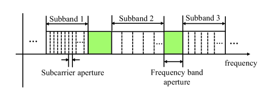
Figure 1: An illustration of subcarrier and frequency band apertures.

Maximum likelihood (ML) based methods: The traditional approaches to estimate the delay parameters are ML based estimation methods, of which the space-alternating generalized expectation-maximization (SAGE) algorithm stands out for its versatility and robustness in harsh multipath environments [25]. In [21], a multiband TOA estimation method has been carried out by the SAGE algorithm for long term evolution (LTE) downlink systems, which provides a reduced standard deviation for the delay estimation. However, the authors in [26] pointed out that the ML based methods tend to converge to a local optimum and need to find the global optimum in a large searching space. To reduce the computational complexity, the authors in [14] proposed a low-complexity approach, which recovers the channel impulse response (CIR) with equally spaced taps and approximately estimates the first path by mitigating the energy leakage. However, this method estimates the delay of the first path coarsely and results in a limited performance improvement.

Subspace based estimation methods: There have been works attempting to solve the multiband delay estimation problems by using subspace based methods, such as multiple signal classification (MUSIC) [20] and estimating signal parameters via rotational invariance techniques (ESPRIT) [18, 19]. In [20], the classical MUSIC algorithm has been applied to delay estimation. However, this approach simply exploits the subcarrier apertures gain while the frequency band apertures gain is not exploited, which results in a performance loss. The authors in [18, 19] employed the multiple shift-invariance structure in the multiband channel measurements and thus the proposed algorithm achieves a high accuracy delay estimation. Nevertheless, the subcarrier spacing of different subbands is assumed to be equivalent, which restricts its applications for practical systems. Moreover, the subspace based methods generally require multiple snapshots of orthogonal frequency division multiplexing (OFDM) pilot symbols to guarantee the performance [27], which consumes lots of pilot resources.

Compressed sensing (CS) based methods: In an indoor environment, the CIR is sparse since it consists of only a small number of paths. Motivated by the sparsity of CIR over the delay domain, many state-of-the-art delay estimation algorithms have been proposed based on CS methods [15, 16, 17]. In [15, 16], the authors formulated $l_{1}$-norm minimization problems for capturing the signal sparsity. In [17], orthogonal matching pursuit (OMP) methods have been used for recovering the sparse CIR. However, these approaches have the problem of energy leakage resulting from basis mismatch [28], which require dense grids and have high computational complexity.

In the aforementioned studies, on one hand, the accuracy of most algorithms is limited, since the associated multi-parameter estimation problem contains many bad local optimums caused by high frequency carrier terms and frequency band apertures. Though some other works have eliminated the oscillation, they have not exploited all apertures gains in the multiband CSI measurements [15, 20], e.g., most works only exploit the subcarrier apertures gain due to the difficulty of exploiting the frequency band apertures gain. On the other hand, many works have not considered the imperfect phase distortion factors caused by receiver timing offset or phase noise in practical systems [14, 18, 20, 29]. Though some studies in [15, 17, 19] have considered the phase distortion, the calibration of the phase distortions with extra information is required via a handshaking procedure under the assumption of channel reciprocity. However, this assumption is restrictive and the transceiver needs to have the ability of Tx/Rx switching. Furthermore, in the handshaking procedure, the phase lock loop (PLL) must keep inlock to ensure that the phase offset remain an unchanged absolute value, which is difficult to achieve in practice.

In this paper, we consider a TOA-based localization system using OFDM training signals over multiple frequency subbands. Then, a novel two-stage global estimation (TSGE) scheme is proposed to fully exploit all the multiband gains, where we consider all the phase distortion factors and calibrate them implicitly without using extra handshaking procedures.

Specifically, in Stage 1, we build a coarse signal model, in which the high frequency carriers are all absorbed for eliminating the oscillation of the likelihood function. Although the coarse estimation algorithm derived from the coarse signal model can only exploit the subcarrier apertures gain, it does not get stuck in bad local optimums and thus can provide a much more stable delay estimation to narrow down the search range for the global delay estimation in the refined stage. Then, we provide a sparse representation for multiband CFR, where we adopt a common support based sparse vector to capture the group sparsity structure in the multiband channel over the delay domain. Based on this model, a Turbo Bayesian inference (Turbo-BI) algorithm is proposed for channel parameter estimation (including the delay parameter). Compared to the CS-based delay estimation methods in [15, 16, 17], our proposed algorithm achieves higher estimation accuracy with lower computational complexity. It is because we adopt a dynamic grid adjustment strategy and we do not need a very dense grid.

In Stage 2, with the help of prior information passed from Stage 1, we perform a finer estimation based on a refined signal model. A higher estimation accuracy than that in Stage 1 can be guaranteed since this signal model contains the structure of frequency band apertures. However, the refined signal model leads to a multi-dimensional non-convex likelihood function that has many bad local optimums, which makes it extremely difficult to find the global optimum and fully exploit the frequency band apertures gain. For utilizing this apertures gain and the prior information properly, we adopt a global search algorithm based on the particle swarm optimization (PSO) to find a good solution for the non-convex optimization of the multi-dimensional likelihood function. In particular, the coarse estimation results from Stage 1 can be utilized for determining the particle search range, which can reduce the search complexity significantly. For further reducing the search space and improving the estimation accuracy, we employ primal-decomposition theory to decouple the objective function and get a least square (LS) solution for channel coefficients. Then, the dimension of the search space can be reduced by eliminating the channel coefficients in the primal optimization problem. The main contributions are summarized below.

• A novel TSGE scheme is proposed for obtaining multiband gains with acceptable complexity, which includes a coarse estimation stage and a refined estimation stage based on a two-stage signal model.

• In Stage 1, we set up a common support based probability model, which employs the group sparsity structure of the multiband channel. Then, a Turbo-BI algorithm is proposed for delay estimation.

• In Stage 2, we propose a PSO-LS algorithm based on PSO and primal-decomposition theory, which reduces the dimension of the search space and significantly improves the estimation accuracy.

Finally, extensive simulation results are presented to validate the effectiveness of the proposed scheme and we show that it can achieve superior delay estimation accuracy as compared to the baseline schemes.

The rest of this paper is organized as follows. In Section II, we describe the system model and introduce the phase distortion factors. In Section III, we formulate the two-stage signal model and outline the TSGE scheme. Sections IV and V present the Turbo-BI algorithm and the PSO-LS algorithm in Stage 1 and Stage 2, respectively. In Section VI, numerical results are presented and finally Section VII concludes the paper.

Notations: Bold upper (lower)-case letters are used to define matrices (column vectors). In particular, bold letters indexed by subscript $m$ denote vectors or matrices corresponding to the $m$-th subband. $\mathbf{I}$ denotes an identity matrix, $\delta\left(\cdot\right)$ denotes the Dirac’s delta function, $\mathrm{diag}\left(\cdot\right)$ constructs a diagonal matrix from its vector argument, and $\|\cdot\|$ denotes the Euclidean norm of a complex vector. For a matrix $\mathbf{A}$, $\mathbf{A}^{T},\mathbf{A}^{H},\mathbf{A}^{-1},\mathrm{tr}(\mathbf{A})$ represent a transpose, complex conjugate transpose, inverse, and trace of a matrix, respectively. For a scalar $a$, $a^{*}$ denotes the conjugate of a scalar. The notation $\mathbb{R}^{\textrm{+}}$ represents the strictly positive real number and $\mathcal{CN}(\mathbf{x};\mathrm{\boldsymbol{\mu}},\boldsymbol{\Sigma})$ denotes a complex Gaussian normal distribution corresponding to variable $\mathbf{x}$ with mean $\boldsymbol{\mu}$ and covariance matrix $\boldsymbol{\Sigma}$.

II System Model

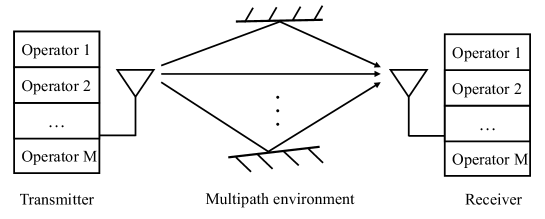
Figure 2: An illustration of the multiband OFDM system.

As shown in Fig. 2, we consider a single-input single-output (SISO) multiband system which employs OFDM training signals over $M$ frequency subbands. The multiband system consists of $M$ non-overlapping single band OFDM subsystems, where the $m$-th subband is allocated to the $m$-th operator. Assume that each frequency subband has $N_{m}$ orthogonal subcarriers with subcarrier spacing $f_{s,m}$ and the carrier frequency of subband $m$ is denoted as $f_{c,m}$. Then, the continuous-time CIR $h\left(t\right)$ can be written as

$$h(t)=\sum_{k=1}^{K}\alpha_{k}\delta\left(t-\tau_{k}\right),$$ (1)

where $K$ denotes the number of multipath components between the transmitter and the receiver, $\alpha_{k}\in\mathbb{C}$ and $\tau_{k}\in\mathbb{R^{\textrm{+}}}$ denote the complex path gain and the delay of the $k$-th path, respectively. The delays are sorted in an increasing order, i.e., $\tau_{k-1}<\tau_{k}$, $k=2,...,K$, and $\tau_{1}$ is the LoS path which needs to be estimated for localization. We assume that the complex path gain and delay parameters are independent of the frequency subbands. Then, via a Fourier transform of the CIR as in [16, 19], the CFR samples can be expressed as

$$\tilde{h}_{m,n}=\sum_{k=1}^{K}\alpha_{k}e^{-j2\pi f_{m,n}\tau_{k}},$$ (2)

where $f_{m,n}=f_{c,m}+n_{m}f_{s,m}$, $m=1,...,M$, $n_{m}\in\mathcal{N_{\mathit{m}}}\triangleq\left\{-\frac{N_{m}}{2},...,\frac{N_{m}}{2}-1\right\}$. With a slight abuse of notation, we use $n$ instead of $n_{m}$ in the following equations. We assume that $N_{\mathit{m}},\forall m$ is an even number without loss of generality, and denote $N=N_{1}+\ldots+N_{M}$ as the number of CFR samples over all subbands.

Apparently, the CFR exhibits sparsity over delay domain when $K$ is small, which will be exploited in our proposed Turbo-BI algorithm. Then, during the period of a single OFDM symbol, the discrete-time received signal model can be written as [16, 19]

$$y_{m,n}=\sum_{k=1}^{K}\alpha_{k}e^{-j2\pi\left(f_{c,m}+nf_{s,m}\right)\tau_{k}}e^{-j2\pi nf_{s,m}\delta_{m}}e^{j\varphi_{m}}s_{m,n}+w_{m,n},$$ (3)

where $w_{m,n}$ is the $n$-th element of the additive white Gaussian noise (AWGN) vector $\boldsymbol{w}_{m}\in\mathbb{C}^{N_{m}\times 1}$, following the distribution $\mathcal{C}\mathcal{N}\left(0,\sigma_{ns}^{2}\mathbf{I}\right)$. $s_{m,n}$ denotes a known training symbol over the $n$-th subcarrier of subband $m$ and we assume $s_{m,n}=1,\forall m,n$ for simplicity. The parameter $\varphi_{m}$ and $\delta_{m}$ represent the phase distortion factors caused by random phase offset and receiver timing offset [22, 23, 24], respectively. In practice, the receiver timing offset $\delta_{m}$ is often within a small range and thus we assume that $\delta_{m},\forall m$ follows a prior distribution $p\left(\delta_{m}\right)\sim\mathcal{N}\left(0,\sigma_{p}^{2}\right)$ [24], where $\sigma_{p}$ is the timing synchronizaton error.

However, the global delay estimation problem will be intractable if we directly use the signal model (3) due to the huge search space of the multi-dimensinal parameters and the existence of many local optimums in the likelihood function, which thus motivates the set up of the novel two-stage signal model and the associated two-stage global estimation scheme.

III Two-Stage Global Estimation Scheme for Multiband Delay Estimation

In this section, we first explain why we cannot use the original signal model for delay estimation based on the likelihood function analysis, which motivates us to introduce the proposed two-stage signal model. Then, based on the two-stage signal model, we provide the outline of the proposed TSGE scheme.

III-A Two-Stage Signal Model

It is difficult to directly use the received signal model (3) for delay estimation. On one hand, the original model (3) exists inherent ambiguity. Specifically, for an arbitrary constant $c$, if we substitute two sets of variables $(\left|\alpha_{k}\right|e^{j\angle\alpha_{k}},\phi_{m})$ and $(\left|\alpha_{k}\right|e^{j(\angle\alpha_{k}+c)},\phi_{m}-c)$ into equation (3), the same observation result will be obtained. It indicates that the parameters $(\alpha_{k},\phi_{m})$ are ambiguous, which leads to the difficulty of delay estimation.

On the other hand, due to the high frequency carrier $f_{c,m}$, the original signal model (3) leads to a multimodal non-convex likelihood function that has many sidelobes. Consequently, it is extremely difficult to find the global optimum. In the worst case, the point of true values may fall into sidelobes, which will inevitably result in a large estimation error. To clarify this problem, we plot a likelihood function curve for the one-dimensional problem of estimating the LoS path delay only in Fig. 3, where the red circle marks the point of the true values of LoS path delay and the red star marks the point of global optimum. As can be seen, the likelihood function fluctuates frequently, which makes it intractable to find the global optimum. Moreover, the point of true values is not in the mainlobe, at which the global optimum locates. Even though we try our best to find the global optimum, an absolute estimation error about $27$ ns is still inevitable.

Therefore, we build new signal models without inherent ambiguity and the probability that the point of true values is in the region of the mainlobe is much higher. Moreover, the signal models should reserve the structure of frequency band apertures and subcarrier apertures. Motivated by the above facts, we propose a two-stage signal model, which is transformed from the original signal model (3) by absorbing different frequency/phase terms into the complex gain.

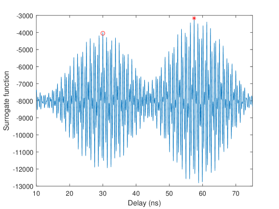
Figure 3: An illustration of the likelihood function based on signal model (3).

III-A1 Coarse Signal Model

$$y_{m,n}=\sum_{k=1}^{K}\alpha_{k,m}e^{-j2\pi nf_{s,m}\tau_{k}}e^{-j2\pi nf_{s,m}\delta_{m}}+w_{m,n},$$ (4)

where $\alpha_{k,m}=\alpha_{k}e^{j\varphi_{m}}e^{-j2\pi f_{c,m}\tau_{k}},\forall k,m$. In signal model (4), we absorb the terms of random phase offset $e^{j\varphi_{m}}$ and carrier phase $e^{-j2\pi f_{c,m}\tau_{k}}$ into $\alpha_{k}$. Signal model (4) becomes unambiguous according to this equivalent transformation and all subbands share the common sparse delay domain. As shown in Fig. 4, we depict the likelihood function based on signal model (4) with the same parameter values as Fig. 3. The likelihood function no longer frequently fluctuates and the point of true values locates at the mainlobe region. In this case, we can exploit the subcarrier apertures gain and estimate delay parameters without ambiguity. This helps to achieve a much more stable delay estimation in the coarse estimation stage whose primary purpose is to narrow down the search range to a relatively small region with high stability (probability). However, the estimation accuracy is limited, since we have absorbed the carrier phase term and thus cannot exploit the frequency band apertures gain, which motivates the next refined estimation signal model (5) in Stage 2.

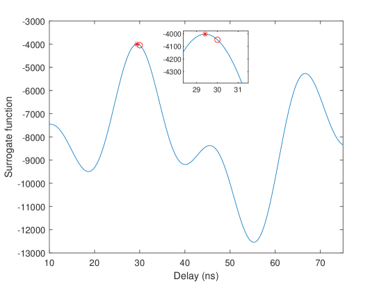
Figure 4: An illustration of the likelihood function based on signal model (4).

III-A2 Refined Signal Model

$$y_{m,n}=\sum_{k=1}^{K}\alpha_{k}^{\prime}e^{-j2\pi f_{c,m}^{\prime}\tau_{k}}e^{-j2\pi nf_{s,m}\tau_{k}}e^{-j2\pi nf_{s,m}\delta_{m}}e^{j\varphi_{m}^{\prime}}+w_{m,n},$$ (5)

where $f_{c,m}^{\prime}=f_{c,m}-f_{c,1}$, $\alpha_{k}^{\prime}=\alpha_{k}e^{j\varphi_{1}}e^{-j2\pi f_{c,1}\tau_{k}}$, $\varphi_{m}^{\prime}=\varphi_{m}-\varphi_{1}$,$\forall k,m.$ In the signal model (5), we absorb the random phase offset, $e^{j\varphi_{1}}$, and carrier phase of the first frequency subband, $e^{-j2\pi f_{c,1}\tau_{k}}$, into $\alpha_{k}$ and reserve the residual term, e.g., $e^{-j2\pi\left(f_{c,2}-f_{c,1}\right)\tau_{k}}$ and $e^{j\left(\varphi_{2}-\varphi_{1}\right)}$ when $m=2$, in (5). Compared to (4), signal model (5) has the extra structure of frequency band apertures, $e^{-j2\pi f_{c,m}^{\prime}\tau_{k}}$, and residual random phase offset, $e^{j\varphi_{m}^{\prime}}$. Fig. 5 illustrates the likelihood function based on signal model (5), where the likelihood function fluctuates less than that in Fig. 3 and the point of true values is now in the mainlobe region. Moreover, we observe that the mainlobe is sharper than that in Fig. 4 due to the the existing of frequency band apertures, which leads to a potential performance improvement. However, the frequency band apertures also cause numerous bad local optimums in the likelihood function. How to find the global optimum with low-complexity is a challenging problem. To solve this problem, we propose the PSO-LS algorithm later.

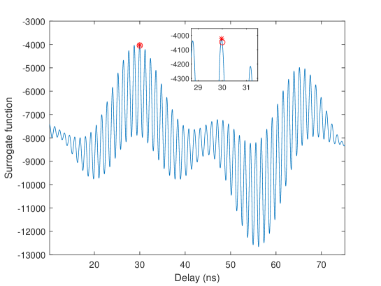
Figure 5: An illustration of the likelihood function based on signal model (5).

In summary, both two signal models are essential. In Stage 1 based on signal model (4), we exploit the subcarrier apertures and give a stable coarse estimation as the initial result to Stage 2. Then, in Stage 2, signal model (5) is used for providing a refined estimation by exploiting both the subcarrier apertures gain and the frequency band apertures gain.

III-B Outline of the TSGE Scheme

Based on the two-stage signal model, the TSGE scheme is depicted as follows:

• Stage 1: We set up the coarse signal model (4) and perform an initial delay estimation using the proposed Turbo-BI algorithm. By doing this, we exploit the channel sparsity over delay domain and the subcarrier apertures gain. Then, we provide the estimation result to Stage 2.

• Stage 2: Based on the coarse estimation result from Stage 1 and the refined signal model (5), a more refined delay estimation is performed. To fully exploit subcarrier and frequency band apertures gains and overcome the difficulty of finding the global optimum as shown in Fig. 5, we propose the PSO-LS algorithm.

The overall algorithm is summarized as in Algorithm 1. The details of the Turbo-BI and PSO-LS algorithms are presented in Section IV and V, respectively.

Algorithm 1 TSGE scheme

Input: CFR samples $y_{m,n},\forall m,n$.

Output: The delay estimation result from Stage 2.

1:  Stage 1:

2:  %Coarse estimation

3:  Construct the coarse signal model (4).

4:  Common support based sparse representation for the coarse signal model (4).

5:  Perform Turbo-BI algorithm.

6:  Pass the coarse estimation result to Stage 2.

7:  Stage 2:

8:  %Refined estimation

9:  Construct the refined signal model (5).

10:  Perform primal-decomposition for problem (27).

11:  Perform PSO-LS algorithm with the the initial particles generated using the coarse estimation in Stage 1.

IV Turbo-BI Algorithm in Stage 1

IV-A Common Support Based Sparse Representation

We first describe the sparse representation over delay domain for the coarse signal model (4), which is a necessary step before employing the sparse recovery methods, e.g., Turbo-BI algorithm. One commonly used method is to define a uniform grid $\mathcal{D}=\left\{\overline{d}_{1},\ldots,\overline{d}_{L}\right\}$ of $L$ ($L\gg K$) delay points over $\left[0,T_{d}\right]$ ($T_{d}$ denotes an upper bound for the maximum delay spread). If all the true delay values exactly lie in the discrete set $\mathcal{D}$, we can reformulate the signal model (4) as:

$$\left[\begin{array}[]{c}\mathbf{y}_{1}\\ \vdots\\ \mathbf{y}_{M}\end{array}\right]=\left[\begin{array}[]{lll}\mathbf{S}_{1}\\ &\ddots\\ &&\mathbf{S}_{M}\end{array}\right]\cdot\left[\begin{array}[]{ccc}\mathbf{A}_{1}\\ &\ddots\\ &&\mathbf{A}_{M}\end{array}\right]\cdot\left[\begin{array}[]{c}\mathbf{x}_{1}\\ \vdots\\ \mathbf{x}_{M}\end{array}\right]+\left[\begin{array}[]{c}\boldsymbol{w}_{1}\\ \vdots\\ \boldsymbol{w}_{M}\end{array}\right],$$ (6)

where $\mathbf{y}_{m}=[y_{m,-\frac{N_{m}}{2}},\cdots,y_{m,\frac{N_{m}}{2}-1}]^{T}\in\mathbb{C}^{N_{m}\times 1}$, $\mathbf{A}_{m}=[\mathbf{a}_{m}(\overline{d}_{1}),\mathbf{a}_{m}(\overline{d}_{2}),\cdots,\mathbf{a}_{m}(\overline{d}_{L})]\in\mathbb{C}^{N_{m}\times L}$ denotes the basis matrix, $\mathbf{a}_{m}(\overline{d}_{l})=[e^{-j2\pi(-\frac{N_{m}}{2})f_{s,m}\overline{d}_{l}},\ldots,e^{-j2\pi(\frac{N_{m}}{2}-1)f_{s,m}\overline{d}_{l}}]^{T}\in\mathbb{C}^{N_{m}\times 1}$ is a linear steering vector, $\mathbf{S}_{m}=\mathrm{diag}(e^{-j2\pi(-\frac{N_{m}}{2})f_{s,m}\delta_{m}},\ldots,$$e^{-j2\pi(\frac{N_{m}}{2}-1)f_{s,m}\delta_{m}})\in\mathbb{C}^{N_{m}\times N_{m}}$, and $\mathbf{x}_{m}\in\mathbb{C}^{L\times 1}$ is a sparse vector whose non-zero elements correspond to the true delays. For example, if the $l$-th element of $\mathbf{x}_{m}$ denoted by $x_{m,l}$ is non-zero and the corresponding true delay is $\tau_{\hat{k}}$, then we have $\overline{d}_{l}=\tau_{\hat{k}}$ and $x_{m,l}=\alpha_{\hat{k},m}$.

However, the true delays generally do not lie exactly on the predefined discrete grid $\mathcal{D}$ in practice, which leads to the energy leakage [28]. To handle this issue, the authors in [15, 16, 17] employ a dense grid ($L\gg N$) to make the equation (6) hold approximately, which leads to a high computational complexity. To overcome the energy leakage caused by delay mismatch and high computational complexity issues of using fixed grids, we adopt a dynamic grid adjustment strategy. Specifically, we introduce an off-grid vector $\Delta\mathbf{\boldsymbol{\tau}}=\left[\Delta\tau_{1},\cdots,\Delta\tau_{L}\right]$, which satisfies $\Delta\tau_{l_{k}}=\tau_{k}-\overline{d}_{l_{k}},k=1,\cdots,K$ and $\Delta\tau_{l}=0,\forall l\notin\left\{l_{1},\cdots,l_{K}\right\}$. Note that $l_{k}\triangleq\underset{l}{\mathrm{argmin}}\left|\tau_{k}-\overline{d}_{l}\right|$ denotes the index of grid which is nearest to $\tau_{k}$. Then, $\mathbf{A}_{m}$ can be rewritten as

$$\mathbf{A}_{m}\left(\Delta\mathbf{\boldsymbol{\tau}}\right)=\left[\mathbf{a}_{m}\left(\overline{d}_{1}+\Delta\tau_{1}\right),\mathbf{a}_{m}\left(\overline{d}_{2}+\Delta\tau_{2}\right),\cdots,\mathbf{a}_{m}\left(\overline{d}_{L}+\Delta\tau_{L}\right)\right].$$ (7)

Now, the mismatch can be compensated by the off-grid vector $\Delta\boldsymbol{\tau}$ and signal model (6) can be held even if the true delays do not lie on the uniform grid $\mathcal{D}$.

After the sparse representation, we propose a support-based probability model to capture the structured sparsity of the multiband channels. Since all sparse vectors $\mathbf{x}_{m}$’s share a common support corresponding to the true delays, the sparse vector $\mathbf{x}=\left[\mathbf{x}_{1};\ldots;\mathbf{x}_{M}\right]$ obeys a group sparsity. We use $\mathbf{s}=\left[s_{1},\ldots,s_{L}\right]^{T}\in\left\{0,1\right\}^{L}$ to denote the common support vector of $\mathbf{x}_{m},\forall m$, where $s_{l}=1$ indicates that $x_{m,l},\forall m$ are active (non-zero), while $s_{l}=0$ indicates that $x_{m,l},\forall m$ are inactive (zero). Then, we further model the channel prior information using a Bernoulli-Gaussian (BG) model [30, 31]. Given the channel support vector, $\mathbf{s}$, the conditional prior distribution of the elements of $\mathbf{x}_{m},\forall m$ is independent and can be written as

$$p\left(x_{m,l}\mid s_{l}\right)=\left(1-s_{l}\right)\delta\left(x_{m,l}\right)+s_{l}\mathcal{CN}\left(x_{m,l};0,\sigma_{m,l}^{2}\right).$$ (8)

IV-B Turbo-BI Algorithm

To achieve the goal of delay estimation, we need to estimate the sparse vector $\mathbf{x}$, support vector $\mathbf{s}$, and the uncertain parameters $\mathbf{\boldsymbol{\xi}}\triangleq[\boldsymbol{\delta}^{T},(\Delta\boldsymbol{\mathbf{\tau}})^{T}]^{T}$, where $\boldsymbol{\delta}=\left[\delta_{1},\ldots,\delta_{M}\right]^{T}$, given the observations $\mathbf{y}=\left[\mathbf{y}_{1};\ldots;\mathbf{y}_{M}\right]\in\mathbb{C}^{N\times 1}$. In particular, for given $\boldsymbol{\xi}$, we are interested in computing the conditional marginal posteriors $p(\mathbf{x}|\mathbf{y},\mathbf{\boldsymbol{\xi}})$. For the uncertain parameters $\boldsymbol{\xi}$, we adopt the maximum a posteriori (MAP) estimation method as

$$\boldsymbol{\xi}^{*}=\underset{\boldsymbol{\xi}}{\mathrm{argmax}}\thinspace p(\boldsymbol{\xi}|\mathbf{y})\propto\underset{\boldsymbol{\xi}}{\mathrm{argmax}}\thinspace\ln p(\mathbf{y},\boldsymbol{\xi})=\underset{\boldsymbol{\xi}}{\mathrm{argmax}}\thinspace\ln\underset{\mathbf{s}}{\sum}\int p(\mathbf{y},\boldsymbol{\xi},\mathbf{x},\mathbf{s})d\mathbf{x}.$$ (9)

This is a high-dimensional non-convex objective function and we cannot obtain a closed-form expression due to the multi-dimensional integration over $\mathbf{x}$ and $\mathbf{s}$, which makes it difficult to directly maximize $\ln p(\mathbf{y},\boldsymbol{\xi})$. To handle this issue, we adopt the majorization-minimization (MM) method to construct a surrogate function and then use alternating optimization (AO) method to find a stationary point of (9). Inspired by the expectation-maximization (EM) method [32], we propose a Turbo-BI algorithm which performs iterations between the following two steps until convergence.

• Turbo-BI-E Step: For given $\mathbf{\boldsymbol{\xi}}$, approximately calculate the posterior $p(\mathbf{x}|\mathbf{y},\mathbf{\boldsymbol{\xi}})$ by combining the message passing and linear minimum mean square error (LMMSE) approaches via a turbo framework, as will be elaborated in Subsection IV-B1;

• Turbo-BI-M Step: Given $p(\mathbf{x}|\mathbf{y},\mathbf{\boldsymbol{\xi}})$, construct a surrogate function for $\ln p(\mathbf{y},\boldsymbol{\xi})$ based on the MM method, partition $\boldsymbol{\xi}$ into $B$ blocks $\mathbf{\boldsymbol{\xi}}=(\mathbf{\boldsymbol{\xi}}_{1},...,\boldsymbol{\xi}_{B})$, then alternatively maximize the surrogate function with respect to $\mathbf{\boldsymbol{\xi}_{\mathit{j}}},j=1,\ldots,B$, as will be elaborated in Subsection IV-B2.

IV-B1 Turbo-BI-E Step

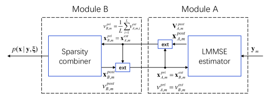
Figure 6: Modules of the Turbo-BI-E step and message flow between different modules.

The Turbo-BI-E step contains two modules, as illustrated in Fig. 6. Module A is a LMMSE estimator based on the observation $\mathbf{y}_{m},\forall m$ and Module B is a sparsity combiner that utilizes the sparsity information of $\mathbf{x}_{m},\forall m$ to further refine the estimation results. The extrinsic estimation of one module will be treated as a prior mean for the other module in the next iteration. Based on the iterations between these two modules, the channel prior information and observations information are combined to be exploited. Specifically, in Module A, we assume that $\mathbf{x}_{m},\forall m$ follows a Gaussian distribution $\mathcal{CN}\left(\mathbf{x}_{m};\mathbf{x}_{A,m}^{pri},v_{A,m}^{pri}\mathbf{I}\right)$, where $\mathbf{x}_{A,m}^{pri}$ and $v_{A,m}^{pri}$ are the extrinsic message output from Module B. We define $\boldsymbol{\Phi}_{m}=\mathbf{S}_{m}\mathbf{A}_{m}\left(\Delta\mathbf{\boldsymbol{\tau}}\right)\in\mathbb{C}^{N_{m}\times L}$ as the measurement matrix and we can obtain the conditional distribution $p\left(\mathbf{y}_{m}|\mathbf{x}_{m}\right)=\mathcal{CN}\left(\boldsymbol{\Phi}_{m}\mathbf{x}_{m},\sigma_{ns}^{2}\mathbf{I}\right)$. Then, the posterior distribution of $\mathbf{x}_{m}$ is given by $p\left(\mathbf{x}_{m}\mid\mathbf{y}_{m}\right)=\mathcal{C}\mathcal{N}\left(\mathbf{x}_{A,m}^{post},\mathbf{V}_{A,m}^{post}\right)$, where

$$\mathbf{V}_{A,m}^{post}=\left(\frac{\boldsymbol{\Phi}_{\mathit{m}}^{\mathit{H}}\boldsymbol{\Phi}_{m}}{\sigma_{ns}^{2}}+\frac{1}{v_{A,m}^{pri}}\mathbf{I}\right)^{-1},$$ (10)

$$\mathbf{x}_{A,m}^{post}=\mathbf{V}_{A,m}^{post}\left(\frac{\mathbf{x}_{A,m}^{pri}}{v_{A,m}^{pri}}+\frac{\boldsymbol{\Phi}_{m}^{H}\mathbf{y}_{m}}{\sigma_{ns}^{2}}\right).$$ (11)

Note that in [33], the singular value decomposition (SVD) of $\boldsymbol{\Phi}_{m}$ is utilized to reduce the computational complexity of $\mathbf{V}_{A,m}^{post}$, which involves a matrix inverse operation. In our case, however, the complexity of the matrix inverse operation is acceptable. It is because $L\ll N_{m}$, the complexity of the matrix inversion operation, $\mathcal{O}\left(L^{3}\right)$, is relatively low. Finally, we calculate the extrinsic message passing:

$$v_{A,m,i}^{ext}=\left(\frac{1}{v_{A,m,i}^{post}}-\frac{1}{v_{A,m}^{pri}}\right)^{-1},$$ (12)

$$x_{A,m,i}^{ext}=v_{A,m,i}^{ext}\left(\frac{x_{A,m,i}^{post}}{v_{A,m,i}^{post}}-\frac{x_{A,m,i}^{pri}}{v_{A,m}^{pri}}\right),$$ (13)

where $v_{A,m,i}^{post}$ is the $i$-th diagonal element of $\mathbf{V}_{A,m}^{post}$.

In Module B, we assume that $\mathbf{x}_{B,m}^{pri}$ is modeled as an AWGN observation of $\mathbf{x}_{m}$ [34, 35]:

$$\mathbf{x}_{B,m}^{pri}=\mathbf{x}_{m}+\mathbf{z}_{m},$$ (14)

where $\mathbf{z}_{m}\sim\mathcal{C}\mathcal{N}\left(0,v_{B,m}^{pri}\mathbf{I}\right)$ is independent of $\mathbf{x}_{m}$, $\mathbf{x}_{B,m}^{pri}=\mathbf{x}_{A,m}^{ext}$ and $v_{B,m}^{pri}=\frac{1}{L}\sum_{i=1}^{L}v_{A,m,i}^{ext}$ are the extrinsic message from Module A. Based on (14), we combine the sparsity prior information of $\mathbf{x}_{m}$ and the extrinsic messages from Module A, aiming at calculating the posterior distributions $p\left(x_{m,l}\mid\mathbf{x}_{B}^{pri}\right)$ by performing the sum-product message passing (SPMP) [36] over the factor graph, where $\mathbf{x}_{B}^{pri}=[(\mathbf{x}_{B,1}^{pri})^{T},\ldots,(\mathbf{x}_{B,M}^{pri})^{T}]^{T}$. Particularly, the factor graph of the joint distribution $p\left(\mathbf{x}_{B}^{pri},\mathbf{x},\mathbf{s}\right)$ is shown in Fig. 7, where the function expression of each factor node is listed in Table I. At subband $m$, the factor graph is denoted by $\mathcal{G_{\mathit{m}}}$. As can be seen, factor graphs $\mathcal{G_{\mathit{m}}}$’s share the common support vector $\mathbf{s}$.

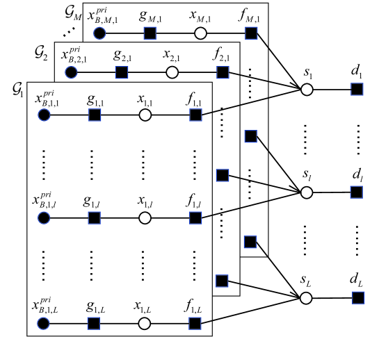
Figure 7: Factor graph of the Turbo-BI algorithm.

TABLE I: Factors, distributions and functional forms in Fig. 7.

Factor	Distribution	Functional form
$g_{m,l}\left(x_{B,m,l}^{pri},x_{m,l}\right)$	$p\left(x_{B,m,l}^{pri}\mid x_{m,l}\right)$	$\mathcal{CN}\left(x_{m,l};x_{B,m,l}^{pri},v_{B,m}^{pri}\right)$
$f_{m,l}\left(s_{l},x_{m,l}\right)$	$p\left(x_{m,l}\mid s_{l}\right)$	$\left(1-s_{l}\right)\delta\left(x_{m,l}\right)+s_{l}\mathcal{CN}\left(x_{m,l};0,\sigma_{m,l}^{2}\right)$
$d_{l}\left(s_{l}\right)$	$p\left(s_{l}\right)$	$p_{s}$

We now outline the message passing scheme on graph $\mathcal{G}$. The details are elaborated in Appendix -A. According to the sum-product rule, the message passing over the path $x_{m,l}\rightarrow f_{m,l}\rightarrow s_{l}$ are given by (33) and (34). Then the message is passed back over the path $s_{l}\rightarrow f_{m,l}\rightarrow x_{m,l}$ using (35) and (36). After calculating the updated messages $\left\{v_{f_{m,l}\rightarrow x_{m,l}}\right\}$, the approximate posterior distributions are given by

$$p\left(x_{m,l}\mid\mathbf{x}_{B}^{pri}\right)\wasypropto v_{f_{m,l}\rightarrow x_{m,l}}\left(x_{m,l}\right)v_{g_{m,l}\rightarrow x_{m,l}}\left(x_{m,l}\right),$$ (15)

where $v_{g_{m,l}\rightarrow x_{m,l}}\left(x_{m,l}\right)=\mathcal{C}\mathcal{N}\left(x_{m,l};x_{B,m,l}^{pri},v_{B,m}^{pri}\right)$. Then the posterior mean and variance are given by

$$x_{B,m,l}^{post}=\mathbb{E}\left(x_{m,l}\mid\mathbf{x}_{B}^{pri}\right)=\int x_{m,l}\thinspace p\left(x_{m,l}\mid\mathbf{x}_{B}^{pri}\right)dx_{m,l},$$ (16)

$$v_{B,m}^{post}=\frac{1}{L}\sum_{l=1}^{L}\mathrm{Var}\left(x_{m,l}\mid\mathbf{x}_{B}^{pri}\right)=\frac{1}{L}\sum_{l=1}^{L}\int\left|x_{m,l}-\mathbb{E}\left(x_{m,l}\mid\mathbf{x}_{B}^{pri}\right)\right|^{2}p\left(x_{m,l}\mid\mathbf{x}_{B}^{pri}\right)dx_{m,l}.$$ (17)

Finally, based on the derivation in [37], the extrinsic update for Module A can be calculated as

$$\mathbf{x}_{A,m}^{pri}=\mathbf{x}_{B,m}^{ext}=v_{A,m}^{pri}\left(\frac{\mathbf{x}_{B,m}^{post}}{v_{B,m}^{post}}-\frac{\mathbf{x}_{B,m}^{pri}}{v_{B,m}^{pri}}\right),$$ (18)

$$v_{A,m}^{pri}=v_{B,m}^{ext}=\left(\frac{1}{v_{B,m}^{post}}-\frac{1}{v_{B,m}^{pri}}\right)^{-1}.$$ (19)

IV-B2 Turbo-BI-M Step

In the M-step, we construct a surrogate function at fixed point $\dot{\boldsymbol{\xi}}$ for the objective function (9) based on the MM method as

$$u(\mathbf{\boldsymbol{\xi}};\dot{\mathbf{\boldsymbol{\xi}}})=\int p(\mathbf{x}\mid\mathbf{y},\dot{\mathbf{\xi}})\ln\frac{p(\mathbf{x},\mathbf{y},\mathbf{\boldsymbol{\xi}})}{p(\mathbf{x}\mid\mathbf{y},\dot{\mathbf{\boldsymbol{\xi}}})}d\mathbf{x},$$ (20)

which satisfies basic properties $u(\boldsymbol{\mathbf{\xi}};\dot{\boldsymbol{\mathbf{\xi}}})\leq\ln p(\mathbf{y},\boldsymbol{\mathbf{\xi}}),\forall\boldsymbol{\mathbf{\xi}}$; $u(\dot{\mathbf{\boldsymbol{\xi}}};\dot{\mathbf{\boldsymbol{\xi}}})=\ln p(\mathbf{y},\dot{\mathbf{\xi}}),\forall\boldsymbol{\mathbf{\xi}}$; $\left.\frac{\partial u(\mathbf{\boldsymbol{\mathbf{\xi}}};\dot{\mathbf{\boldsymbol{\xi}}})}{\partial\boldsymbol{\xi}}\right|_{\mathbf{\boldsymbol{\xi}}=\dot{\mathbf{\boldsymbol{\xi}}}}=\left.\frac{\partial\ln p(\boldsymbol{y},\mathbf{\boldsymbol{\xi}})}{\partial\boldsymbol{\xi}}\right|_{\boldsymbol{\mathbf{\xi}}=\dot{\mathbf{\boldsymbol{\xi}}}},\forall\boldsymbol{\mathbf{\xi}}$. Then, we partition $\mathbf{\boldsymbol{\xi}}$ into $B=2$ blocks with $\boldsymbol{\xi}_{1}=\boldsymbol{\delta}$, $\boldsymbol{\xi}_{2}=\Delta\boldsymbol{\tau}$ based on their distinct physical meaning, and alternatively update $\boldsymbol{\xi}_{1}$ and $\boldsymbol{\xi}_{2}$ as

$$\mathbf{\boldsymbol{\delta}}^{(i+1)} = \underset{\mathbf{\boldsymbol{\delta}}}{\mathrm{argmax}}\thinspace u\left(\mathbf{\boldsymbol{\delta}},\Delta\boldsymbol{\tau}^{(i)};\mathbf{\boldsymbol{\delta}}^{(i)},\Delta\boldsymbol{\tau}^{(i)}\right),$$ (21)

$$\Delta\mathbf{\boldsymbol{\tau}}^{(i+1)} = \underset{\boldsymbol{\Delta}\mathbf{\tau}}{\mathrm{argmax}}\thinspace u\left(\boldsymbol{\delta}^{(i+1)},\Delta\boldsymbol{\tau};\boldsymbol{\delta}^{(i)},\Delta\boldsymbol{\tau}^{(i)}\right).$$ (22)

Since the optimization problems (21) and (22) are non-convex and it is hard to find their optimal solutions, we apply a one-step gradient update for $\mathbf{\boldsymbol{\delta}}$ and $\Delta\boldsymbol{\mathbf{\tau}}$ as follows:

$$\boldsymbol{\delta}^{(i+1)} = \boldsymbol{\delta}^{(i)}+\gamma_{\boldsymbol{\delta}}\cdot\boldsymbol{\zeta}_{\boldsymbol{\delta}}^{(i)},$$ (23)

$$\Delta\boldsymbol{\tau}^{(i+1)} = \Delta\boldsymbol{\tau}^{(i)}+\gamma_{\Delta\boldsymbol{\tau}}\cdot\boldsymbol{\zeta}_{\Delta\boldsymbol{\tau}}^{(i)},$$ (24)

where $\gamma_{\boldsymbol{\delta}}$ and $\gamma_{\Delta\boldsymbol{\tau}}$ are the step size determined by the Armijo rule [38], $\boldsymbol{\zeta}_{\boldsymbol{\delta}}^{(i)}$ and $\boldsymbol{\zeta}_{\Delta\boldsymbol{\tau}}^{(i)}$ are the gradients of the objective function in (21) and (22) with respect to $\boldsymbol{\delta}$ and $\Delta\boldsymbol{\tau}$, respectively. The detailed derivations for $\boldsymbol{\zeta}_{\boldsymbol{\delta}}^{(i)}$ and $\boldsymbol{\zeta}_{\Delta\boldsymbol{\tau}}^{(i)}$ are presented in Appendix -B. Moreover, the convergence of this in-exact MM algorithm to a stationary point can be guaranteed [39, Theorem 1].

IV-C Summary of the Turbo-BI Algorithm and Complexity Analysis

The Turbo-BI algorithm is summarized in Algorithm 2. Finally, we analyze the computational complexity of the proposed Turbo-BI algorithm. It is observed that the computational complexity of the Turbo-BI-E step is dominated by the matrix multiplication $\boldsymbol{\Phi}_{\mathit{m}}^{\mathit{H}}\boldsymbol{\Phi}_{m}$ in (10), which is $\mathcal{O}\left(N_{m}L^{2}\right)$.

In the Turbo-BI-M step, the computational complexity of choosing the right step size mainly depends on calculating the cost function. We denote the number of calculating the cost function for $\gamma_{\boldsymbol{\delta}}$ and $\gamma_{\Delta\boldsymbol{\tau}}$ in every backtracking line search as $R_{b,1}$ and $R_{b,2}$, respectively. Then, the complexity of choosing $\gamma_{\boldsymbol{\delta}}$ and $\gamma_{\Delta\boldsymbol{\tau}}$ are $\mathcal{O}\left(NL^{2}R_{b,1}\right)$ and $\mathcal{O}\left(NL^{2}R_{b,2}\right)$, respectively. Besides, the complexity in calculating $\boldsymbol{\zeta}_{\boldsymbol{\delta}}$ and $\boldsymbol{\zeta}_{\Delta\boldsymbol{\tau}}$ are $\mathcal{O}\left(NL^{2}\right)$ and $\mathcal{O}\left(NL\right)$ based on matrix multiplication, respectively. Hence, the overall computational complexity of Turbo-BI algorithm is $\mathcal{O}\left(NL^{2}I_{in}+NL^{2}(R_{b,1}+R_{b,2})\right)$ per iteration, where $I_{in}$ denotes the number of Turbo iterations for convergence.

Algorithm 2 Turbo-BI algorithm

Input: $\boldsymbol{y}$, $\boldsymbol{\Phi}_{m},\forall m$, maximum iteration number $I_{EM}$, threshold $\epsilon$.

Output: $\boldsymbol{\delta}^{\ast}$, $\Delta\boldsymbol{\tau}^{\ast}$.

1:  for ${\color[rgb]{0,0,1}{\color[rgb]{0,0,0}i=1,\cdots,I_{EM}}}$ do

2:     Turbo-BI-E Step:

3:     while not converge do

4:        %Module A: LMMSE Estimator

5:        Initialize $\mathbf{x}_{A,m}^{pri}=\boldsymbol{0}$ and $v_{A,m}^{pri}$.

6:        Update $\mathbf{V}_{A,m}^{post}$ and $\mathbf{x}_{A,m}^{post}$, using (10) and (11).

7:        Update the extrinsic information $v_{B,m}^{pri}=\frac{1}{L}\sum_{i=1}^{L}v_{A,m,i}^{ext}$ and $\mathbf{x}_{B,m}^{pri}=\mathbf{x}_{A,m}^{ext}$, using (12) and (13).

8:        % Module B: Sparsity Combiner

9:        Perform message passing over the factor graph $\mathcal{G}$ using (33) - (36).

10:        Calculate the approximate posterior distributions $p\left(x_{l}^{m}\mid\mathbf{x}_{B}^{pri}\right)$ using (15).

11:        Update $x_{B,m,l}^{post}$ and $v_{B,m}^{post}$ using (16) and (17).

12:        Update the extrinsic information $\mathbf{x}_{A,m}^{pri}=\mathbf{x}_{B,m}^{ext}$ and $v_{A,m}^{pri}=v_{B,m}^{ext}$, using (18) and (19).

13:     end while

14:     Turbo-BI-M Step:

15:     Construct the surrogate function in (20) using $\mathbf{x}_{A,m}^{post}$ and $\mathbf{V}_{A,m}^{post}$, which is from the Turbo-BI-E step.

16:     Update $\boldsymbol{\delta}$ and $\Delta\boldsymbol{\tau}$, using (23) and (24).

17:     if  $\left\|\Delta\boldsymbol{\delta}^{(i+1)}-\Delta\boldsymbol{\delta}^{(i)}\right\|\leq\epsilon$ and $\left\|\Delta\boldsymbol{\tau}^{(i+1)}-\Delta\boldsymbol{\tau}^{(i)}\right\|\leq\epsilon$ then

18:        break

19:     end if

20:  end for

V PSO-LS Algorithm in Stage 2

In Stage 2, we aim to fully exploit the frequency band apertures gain and perform a refined delay estimation based on the estimation result from Stage 1. First, we reformulate the refined estimation signal model (5) as a linear form:

$$\mathbf{y}=\mathbf{H\left(\boldsymbol{\theta}\right)x}+\boldsymbol{w},$$ (25)

where $\mathbf{H\left(\boldsymbol{\theta}\right)}=\left[\begin{array}[]{ccc}\mathbf{h}_{11}&\cdots&\mathbf{h}_{1K}\\ \vdots&\ddots&\vdots\\ \mathbf{h}_{M1}&\cdots&\mathbf{h}_{MK}\end{array}\right]\in\mathbb{C}^{N\times K}$, $h_{mk}(n)=e^{-j2\pi\left(f_{c,m}^{\prime}+nf_{s,m}\right)\tau_{k}}e^{-j2\pi nf_{s,m}\delta_{m}}e^{j\varphi_{m}^{\prime}}$ denotes the $n$-th element of the column vector $\mathbf{h}_{mk}$, $\mathbf{\boldsymbol{\theta}}=[\tau_{1},...,\tau_{K},$$\delta_{1},...,\delta_{M},\varphi_{2}^{\prime},...,\varphi_{M}^{\prime}]^{T}\in\mathbb{R}^{(K+2M-1)\times 1}$ denotes the vector consisting of unknown parameters, $\mathbf{x}=\left[\alpha_{1}^{\prime},\ldots,\alpha_{K}^{\prime}\right]^{T}\in\mathbb{C}^{K\times 1}$, and $\boldsymbol{w}\sim\mathcal{C}\mathcal{N}(0,\sigma_{ns}^{2}\mathbf{I})\in\mathbb{C}^{N\times 1}$. We adopt the MAP method for estimation, that takes the prior information of $\delta_{m}$ into consideration. Then, the optimization problem can be formulated as

$$\mathcal{P}_{1}: \underset{\boldsymbol{\theta},\mathbf{x}}{\max} \ln\thinspace p\left(\mathbf{y}|\mathbf{x}\right)+\sum_{m=1}^{M}\textrm{ln}\thinspace p\left(\delta_{m}\right)$$ (26)

s.t. $$0\leq\varphi_{m}^{\prime}\leq 2\pi,\forall m\in\left\{2,\cdots,M\right\},$$

where $p\left(\mathbf{y}|\mathbf{x}\right)\wasypropto e^{-\frac{\|\mathbf{y}-\mathbf{H\left(\theta\right)x}\|^{2}}{\sigma_{ns}^{2}}}$ is the likelihood function. After an equivalent transformation, $\mathcal{P}_{1}$ can be reformulated as

$$\mathcal{P}_{2}: \underset{\boldsymbol{\theta},\mathbf{x}}{\min} \frac{\|\mathbf{y}-\mathbf{H\left(\boldsymbol{\theta}\right)x}\|^{2}}{\sigma_{ns}^{2}}+\sum_{m=1}^{M}\frac{\delta_{m}^{2}}{2\sigma_{p}^{2}}$$ (27)

s.t. $$0\leq\varphi_{m}^{\prime}\leq 2\pi,\forall m\in\left\{2,\cdots,M\right\}.$$

The non-convex problem $\mathcal{P}_{2}$ has a multimodal and multi-dimensional objective function, which is extremely challenging to solve due to the existence of numerous local optimums. In this case, conventional algorithms, such as gradient descent and exhaustive search algorithms, have high-computational complexity or are easily trapped into local optimums. To overcome these drawbacks, we adopt the PSO method [40, 41, 42, 43] to find a good solution for the non-convex optimization problem $\mathcal{P}_{2}$.

In the PSO method, we employ a number of particles which are potential solutions, to find the optimal solution by iterations, where the search space is bounded by the constraints of the target optimization problem [44]. This heuristic algorithm has been shown to have low computational complexity and a strong optimization ability for complex multimodal optimization problems [42]. Generally, PSO starts with a random initialization of the particles’ locations in a large search space. In our problem $\mathcal{P}_{2}$, however, we can narrow down the search space based on the coarse estimation results from Stage 1.

Specifically, we set the search space as

$$\mathcal{S}=[\boldsymbol{\beta}-\mathbf{e},\boldsymbol{\beta}+\mathbf{e}]\in\mathbb{R}^{D\times 1},$$ (28)

where $\boldsymbol{\beta}$ has the values consisting of the coarse estimation results, $\mathbf{e}$ is the search range obtained by evaluating the mean squared error (MSE) of coarse estimation results based on offline training or evaluating the Cramï¿œr-Rao bound (CRB) values based on coarse signal model (4), and $D$ denotes the dimension of the particles (search space). Since there is no estimation for $\varphi_{m}^{\prime}$ in Stage 1, the search space for $\varphi_{m}^{\prime}$ is set to be $\left[0,2\pi\right]$. Note that the search space $S$ is a real set with dimension $D=3K+2M-1$, since the $K$-dimension complex vector $\mathbf{x}$ can be seen as a $2K$-dimension real vector in a real domain search space. Then, for the $i$-th iteration, each particle comes to a better location by updating its velocity and position based on the following two equations:

$$V_{q,d}^{(i+1)}=\omega V_{q,d}^{(i)}+c_{1}r_{1,q,d}\left(pbest_{q,d}^{(i)}-X_{q,d}^{(i)}\right)+c_{2}r_{2,q,d}\left(gbest_{d}^{(i)}-X_{q,d}^{(i)}\right),$$ (29)

$$X_{q,d}^{(i+1)}=X_{q,d}^{(i)}+V_{q,d}^{(i+1)},$$ (30)

where $c_{1}$ and $c_{2}$ are acceleration coefficients, and $\omega$ is the inertia factor, which is proposed to balance the global and local search abilities [45]. Note that $X_{q,d}^{(i)}$ and $V_{q,d}^{(i)}$ are the position and velocity of the $d$-th element of the $q$-th particle, respectively, where $q\in\left\{1,2,...,Q_{p}\right\},d\in\left\{1,2,...,D\right\}$ with $Q_{p}$ denoting the number of particles. $r_{1,q,d}$ and $r_{2,q,d}$ are two independent random numbers uniformly distributed within $[0,1]$. Besides, $gbest$ denotes the best position in the whole swarm and $pbest_{q,d}^{(i)}$ denotes the best position values at the $d$-th dimension that the $q$-th particle has come across so far at the $i$-th iteration. The goodness of the particle position is measured by the objective function value in $\mathcal{P}_{2}$ (also called fitness in PSO algorithms). In our problem, a smaller fitness indicates a better position.

For getting a better solution in the PSO algorithm, we aim to reduce the dimension of the search space in problem $\mathcal{P}_{2}$ and thus propose the PSO-LS algorithm. We first employ primal-decomposition theory to decouple the problem $\mathcal{P}_{2}$ as:

$$\mathcal{P}_{3}: \underset{\boldsymbol{\theta}}{\min} \frac{\|\mathbf{y}-\mathbf{H\left(\boldsymbol{\theta}\right)\mathit{g}^{*}(\boldsymbol{\theta})}\|^{2}}{\sigma_{ns}^{2}}+\sum_{m=1}^{M}\frac{\delta_{m}^{2}}{2\sigma_{p}^{2}}$$ (31)

s.t. $$0\leq\varphi_{m}^{\prime}\leq 2\pi,\forall m\in\left\{2,\cdots,M\right\},$$

where $g^{*}(\boldsymbol{\theta})=\underset{\mathbf{x}}{\mathrm{argmin}}\|\mathbf{y}-\mathbf{H\left(\boldsymbol{\theta}\right)x}\|^{2}$. Then we can obtain a least-square (LS) solution of $g^{*}(\boldsymbol{\theta})$ as

$$g^{*}(\boldsymbol{\theta})=\left(\mathbf{H\left(\boldsymbol{\theta}\right)}^{H}\mathbf{H\left(\boldsymbol{\theta}\right)}\right)^{-1}\mathbf{H\left(\boldsymbol{\theta}\right)}^{H}\mathbf{y}.$$ (32)

Using this method, the dimension of search space is reduced from $\mathbb{R}^{3K+2M-1}$ to $\mathbb{R}^{K+2M-1}$. Then, we analyze the computational complexity of the PSO-LS algorithm. The complexity mainly depends on the calculations of the objective function in (31), which is $\mathcal{O}\left(NK^{2}Q_{p}\right)$ per iteration. Finally, the proposed PSO-LS algorithm is presented in Algorithm 3.

Algorithm 3 PSO-LS algorithm

Input: $\mathbf{y}$, search space $\mathcal{S}$, $Q_{p}$, maximum iteration number $I_{PSO}$, threshold $\epsilon$.

Output: $\mathbf{gbest}$.

1:  Initialize $X_{q,d}^{(1)}$ within the search space $\mathcal{S}$ in (28), $V_{q,d}^{(1)}$, $gbest_{d}^{(1)}$, $pbest_{q,d}^{(1)}$, $\forall q,d$.

2:  for  $i=1,\cdots,I_{PSO}$ do

3:     for ${\color[rgb]{0,0,1}{\color[rgb]{0,0,0}q=1,\cdots,Q_{p}}}$ do

4:        Update the velocity of particle $q$ using (29).

5:        Update the position of particle $q$ using (30).

6:        Calculate the fitness of particle $q$ based on the objective in (31).

7:        Update $pbest_{q,d}^{(i+1)}$ and $gbest_{d}^{(i+1)}$ ,$\forall q,d$.

8:     end for

9:     if  $\left\|\mathbf{gbest}^{(i+1)}-\mathbf{gbest}^{(i)}\right\|\leq\epsilon$ then

10:        break

11:     end if

12:  end for

VI Simulation Results

In this section, we provide numerical results to evaluate the performance of the proposed schemes and draw useful insights. In the default setup, we consider that CSI samples are collected using one OFDM training symbol with subcarrier spacing $f_{s,1}=f_{s,2}=60$ KHz and subband bandwidth $B_{1}=B_{2}=40$ MHz at $M=2$ subbands, with central frequencies $f_{c,1}=1.80$ GHz and $f_{c,2}=2.02$ GHz. $\varphi_{m},\forall m$ and $\delta_{m},\forall m$ are generated following a uniform distribution within $[0,2\pi]$ and a Gaussian distribution $\mathcal{N}\left(0,\sigma_{p}^{2}\right)$, respectively. We use the Quadriga platform to generate multiband CSI samples in an indoor factory (InF) scenario, which is depicted in 3GPP R16 [46]. Other system parameters are set as follows unless otherwise specified: Signal-to-noise ratio (SNR) is 7 dB, $I_{EM}=100$, $I_{PSO}=500$, $Q_{p}=100$, $\epsilon=10^{-5}$, $c_{1}=2.5$, $c_{2}=0.5$, and $\omega=0.99-\frac{0.79}{I_{PSO}}t$ for the $t$-th PSO iteration. To assess the performance of the schemes, we adopt the empirical cumulative distribution function (CDF) of the LoS path delay estimation errors using 200 Monte Carlo trials.

For comparison, we consider the following four benchmark schemes:

• Turbo-BI algorithm: We adopt the coarse estimation results of the Turbo-BI algorithm in Stage 1 as one of the benchmarks.

• Multiband weighted delay estimation (MBWDE) algorithm [19]: It adopts a weighted subspace fitting algorithm for delay estimation, which is able to exploit the frequency band apertures gain.

• Two-stage gradient descent (TSGD) scheme: This scheme has the same coarse estimation implementation as the TSGE scheme in Stage 1 and then the gradient descent method is employed to perform refined estimation in Stage 2 with the initial point generated using the coarse estimation in Stage 1.

• Ideal gradient descent (IGD) scheme: This scheme adopts gradient descent method based on problem $\mathcal{P}_{2}$, where we set the initial point to be the true values. In fact, this scheme is infeasible because we cannot know the true values of the estimation parameters in practical environment. In the simulations, however, we can regard this scheme as an ideal benchmark to show the effectiveness of the TSGE scheme.

VI-A Impact of the factor $\boldsymbol{\delta}$

We first study the impact of the receiver timing offset $\boldsymbol{\delta}$. Since the InF scenario does not consider the effect of $\boldsymbol{\delta}$, we construct a two-path channel model with Rayleigh distributed magnitudes. The delays are set to follow a uniform distribution within $[20,200]$ ns. Fig. 8 depicts the CDF of LoS path delay estimation errors for different standard deviation $\sigma_{p}$ achieved by TSGE. As can be seen, the factor $\boldsymbol{\delta}$ has significantly degraded the estimation performance. Besides, when $\boldsymbol{\delta}$ is considered, the estimation performance mainly depends on the prior standard deviation $\sigma_{p}$, where the delay estimation errors increase with $\sigma_{p}$. It is reasonable since a larger $\sigma_{p}$ means less prior information of $\boldsymbol{\delta}$ we have. Therefore, in the following simulations, we assume that $\sigma_{p}=0$ ns in order to avoid its effect on the estimation performance.

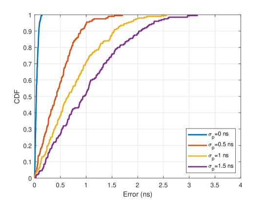
Figure 8: The CDF of LoS path delay estimation errors for different $\sigma_{p}$.

VI-B Performance of TSGE Scheme

In Fig. 9, we compare the delay estimation performance of the TSGE scheme with benchmarks. First, we observe that the CS-based schemes (i.e., TSGE, Turbo-BI, and TSGD) and the IGD scheme achieve a better performance than the subspace-based algorithm, i.e., MBWDE. It is mainly because that the received CSI samples are collected using only a single OFDM training symbol, which leads to a limited ability of subspace-based algorithms to suppress the noise interference. In contrast, CS-based schemes have a strong ability of reducing the effects of noise by signal sparse reconstruction, thus they achieve a better performance. Second, it can be seen that the proposed TSGE scheme significantly outperforms the Turbo-BI and TSGD. This is because TSGE scheme exploits the extra frequency band apertures gain compared to the Turbo-BI algorithm. Moreover, note that the likelihood function based on the refined signal model (5) has numerous local optimums, which requires a strong global search ability for the algorithms in Stage 2. Compared to the gradient descent algorithm in the TSGD scheme, the PSO-LS algorithm in the TSGE scheme has stronger global search ability, thus achieves higher estimation accuracy than TSGD. Finally, it is observed that the CDF curve of TSGE approaches that of IGD, which indicates a negligible performance loss.

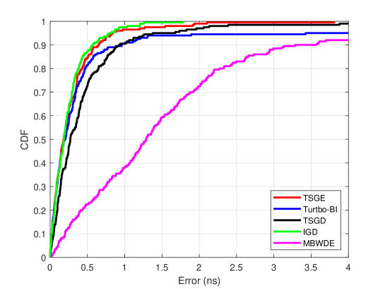
Figure 9: The CDF of LoS path delay estimation errors for different schemes.

In Table II, we investigate the computing cost and the estimation accuracy of the considered algorithms, i.e., the PSO-LS algorithm with different numbers of particles and iterations, primal PSO algorithm based on the problem $\mathcal{P}_{2}$, and the MBWDE algorithm. The computing cost is characterized by the spent CPU time when running the algorithms with the Intel Xeon 6248R CPU. For fairness, we set the same initial estimation values for all algorithms. It can be readily seen that the PSO-LS is able to achieve a higher estimation accuracy with less computing cost than primal PSO, which validates the effectiveness of the proposed PSO-LS algorithms. In addition, our proposed PSO-LS algorithm is able to achieve better estimation accuracy than MBWDE with nearly equal computing cost. Furthermore, we can see that the PSO-LS algorithm is able to achieve a trade-off between the computing cost and estimation performance, which implies that it can be adapted to various scenarios. In particular, when we have sufficient computing resource, we can use a large number of particles and iterations to pursue the highest estimation accuracy. Conversely, when the computing resource is limited, we can use a small number of particles and iterations to achieve a relatively accurate estimation.

TABLE II: CPU time and RMSE comparison.

	PSO-LS ($I_{PSO}=500$,$Q_{p}=100$)	PSO-LS ($I_{PSO}=100$, $Q_{p}=20$)	primal PSO ($I_{PSO}=500$, $Q_{p}=100$)	MBWDE
CPU time (s)	32.8	1.3	20.3	0.8
RMSE (ns)	0.2876	0.5425	0.5517	1.671

VI-C Impact of Frequency Band Spacing

Fig. 10 illustrates the root mean square error (RMSE) of the LoS delay estimation for different schemes versus frequency band spacing, when $\textrm{SNR}=10$ dB and bandwidth $B_{1}=B_{2}=60$ MHz. We define $\mathrm{RMSE}(\hat{\tau})\triangleq\sqrt{\mathbb{E}\left\{(\hat{\tau}-\tau)^{2}\right\}}$, where $\hat{\tau}$ is the estimated LoS delay and $\tau$ is the true LoS delay. In particular, we fix $f_{c,1}$ and change $f_{c,2}$ for different frequency band spacings. It can be seen that the RMSE decreases with the increase of frequency band spacing for MBWDE, TSGE, and IGD. This is because these schemes are able to exploit frequency band apertures gain, which enlarges as frequency band spacing increases. Furthermore, the TSGD scheme has a better performance than the Turbo-BI algorithm when frequency band spacing is narrow, but the performance gap decreases as the frequency band spacing increases. When the frequency band spacing is 260 MHz, the performance of TSGD is even worse than Turbo-BI. This is reasonable since the oscillation of the likelihood function becomes more violent with the increase of frequency band spacing, which causes more bad local optimums and makes it more difficult to fully exploit the frequency band apertures gain. However, TSGD has a limited global search ability, which results in a high probability of being stuck into local optimums. Hence, TSGD can only exploit part of frequency band apertures gain and has a poor delay estimation performance with large frequency band spacing. Besides, TSGE has more stable performance than TSGD due to its strong global optimization ability. Finally, we observe that the performance of Turbo-BI is irrelevant to the frequency band spacing since it only exploits subcarrier apertures gain in Stage 1.

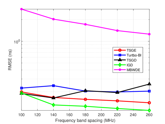
Figure 10: RMSE of LoS delay estimation versus frequency band spacing.

VI-D Impact of SNR

In Fig. 11, we show the impact of SNR on the delay estimation performance. As can be seen, the RMSE of all schemes decreases with the increase of SNR because of the reduction of noise interference to delay estimation. Besides, the performance gap of TSGE and IGD over Turbo-BI becomes larger as SNR increases.

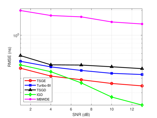
Figure 11: RMSE of LoS delay estimation versus SNR.

VI-E Impact of the Bandwidth

In Fig. 12, we investigate the RMSE of the LoS delay estimation versus the bandwidth with $\textrm{SNR}=10$ dB. It is observed that the delay estimation accuracy increases as the bandwidth, which is mainly because larger bandwidth leads to more subcarrier apertures gain. Furthermore, we observe that the performance gain of TSGE over MBWDE increases with bandwidth.

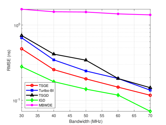
Figure 12: RMSE of LoS delay estimation versus the bandwidth.

VII Conclusion

In this paper, we studied a delay estimation problem in the multiband OFDM system with phase distortion factors considered. We proposed a novel two-stage global estimation scheme that fully exploits the multiband gains to improve the delay estimation performance. In particular, in Stage 1, we perform a common support based sparse representation for the coarse estimation signal model and then achieve a coarse delay estimation using the Turbo-BI algorithm. Then, with the help of the coarse estimation results, we further conducted a more refined delay estimation by employing the proposed PSO-LS algorithm based on the refined signal model in Stage 2. Finally, simulation results showed that the proposed TSGE scheme achieves superior performance over baseline algorithms in the InF scenario. Future work can consider a multiband delay estimation problem for localization in a multiple-input multiple-output (MIMO) system.

-A Message Passing for Module B of Turbo-BI

The message from variable node $x_{m,l}$ to factor node $f_{m,l}$ is given by

$$v_{x_{m,l}\rightarrow f_{m,l}}\left(x_{m,l}\right)=\mathcal{CN}\left(x_{m,l};x_{B,m,l}^{pri},v_{B,m}^{pri}\right).$$ (33)

The message from factor node $f_{m,l}$ to variable node $s_{l}$ is given by

$$v_{f_{m,l}\rightarrow s_{l}}\left(s_{l}\right)\wasypropto\int f_{m,l}\left(x_{m,l},s_{l}\right)v_{x_{m,l}\rightarrow f_{m,l}}\left(x_{m,l}\right)dx_{m,l}=\pi_{l}^{m}\delta\left(s_{l}-1\right)+\left(1-\pi_{l}^{m}\right)\delta\left(s_{l}\right),$$ (34)

where $\pi_{l}^{m}=(1+\frac{\mathcal{C}\mathcal{N}(0;x_{B,m,l}^{pri},v_{B,m}^{pri})}{\mathcal{C}\mathcal{N}(0;x_{B,m,l}^{pri},v_{B,m}^{pri}+\sigma_{m,l}^{2})})^{-1}$. Then the message passed from variable node $s_{l}$ to factor node $f_{m,l}$ is given by

$$v_{s_{l}\rightarrow f_{m,l}}\left(s_{l}\right)\wasypropto v_{d_{l}\rightarrow s_{l}}\left(s_{l}\right)\underset{m^{\prime}\neq m}{\prod}v_{f_{m^{\prime},l}\rightarrow s_{l}}\left(s_{l}\right)=\widehat{\pi}_{l}^{m}s_{l}+\left(1-\widehat{\pi}_{l}^{m}\right)\left(1-s_{l}\right),$$ (35)

where $\widehat{\pi}_{l}^{m}=\frac{p_{s}\prod_{m^{\prime}\neq m}\pi_{l}^{m^{\prime}}}{p_{s}\prod_{m^{\prime}\neq m}\pi_{l}^{m^{\prime}}+(1-p_{s})\prod_{m^{\prime}\neq m}(1-\pi_{l}^{m^{\prime}})}$. Finally, the message passed from factor node $f_{m,l}$ to variable node $x_{m,l}$ is given by

$$v_{f_{m,l}\rightarrow x_{m,l}}\left(x_{m,l}\right)\wasypropto\underset{s_{l}}{\sum}f_{m,l}\left(x_{m,l},s_{l}\right)v_{s_{l}\rightarrow f_{m,l}}\left(s_{l}\right)=\widehat{\pi}_{l}^{m}\mathcal{C}\mathcal{N}\left(x_{m,l};0,\sigma_{m,l}^{2}\right)+\left(1-\widehat{\pi}_{l}^{m}\right)\delta\left(x_{m,l}\right).$$ (36)

-B Gradient Derivation in Turbo-BI-M Step

$$\zeta_{\delta_{m}}=-\frac{2}{\sigma_{ns}^{2}}\mathrm{Re}\left[\mathbf{b}_{m}^{\prime{}^{H}}\mathbf{b}_{m}-\mathbf{b}_{m}^{\prime}{}^{H}\mathbf{y}^{m}+\mathrm{tr}\left(\mathbf{A}_{m}\boldsymbol{\Sigma}_{m}\mathbf{A}_{m}^{H}\mathbf{S}_{m}^{H}\mathbf{S}_{m}^{\prime}\right)\right]-\frac{\delta_{m}}{\sigma_{p}^{2}},$$ (37)

$$\begin{gathered}\zeta_{\Delta\tau_{l}}=-\frac{2}{\sigma_{ns}^{2}}\sum_{m=1}^{M}\mathrm{Re}\left[\left(\left(\mathbf{a}_{m}^{\prime}\left(\overline{d}_{l}+\Delta\tau_{l}\right)\right)^{H}\mathbf{S}_{m}^{H}\mathbf{S}_{m}\mathbf{a}_{m}\left(\overline{d}_{l}+\Delta\tau_{l}\right)\right)\left(\left|\mu_{l,m}\right|^{2}+\Sigma_{ll,m}\right)-\right.\\ \left.\left(\mathbf{a}_{m}^{\prime}\left(\overline{d}_{l}+\Delta\tau_{l}\right)\right)^{H}\mathbf{S}^{H}\left(\mu_{l,m}^{*}\mathbf{y}_{m,-l}-\mathbf{S}_{m}\sum_{j\neq l}\left(\sum_{jl,m}\mathbf{a}_{m}\left(\overline{d}_{l}+\Delta\tau_{j}\right)\right)\right)\right],\end{gathered}$$ (38)

where $\mathbf{b}_{m}=\mathbf{S}_{m}\mathbf{A}_{m}\mu_{m}$, $\mathbf{b}_{m}^{\prime}=\frac{\partial\mathbf{b}_{m}}{\partial\delta_{m}}$, $\mathbf{y}_{m,-l}=\mathbf{y}_{m}-\mathbf{S}_{m}\sum_{j\neq l}(\mu_{j,m}\mathbf{a}_{m}(\overline{d}_{j}+\Delta\boldsymbol{\tau}_{j}))$, $\mathbf{a}_{m}^{\prime}(\overline{d}_{l}+\Delta\boldsymbol{\tau}_{l})=\frac{d\mathbf{a}_{m}(\overline{d}_{l}+\Delta\boldsymbol{\tau}_{l})}{d\Delta\boldsymbol{\tau}_{l}}$, $\mathbf{S}_{m}^{\prime}=\frac{d\mathbf{S}_{m}}{d\delta_{m}}$, $\mu_{l,m}$ and $\Sigma_{jl,m}$ denote the $l$-th element and the $(j,l)$-th element of the posterior mean $\boldsymbol{\mu}_{m}$ and covariance $\boldsymbol{\Sigma}_{m}$ associated with $p(\mathbf{x}\mid\mathbf{y},\boldsymbol{\xi})$, which can be approximated using the $\mathbf{x}_{A,m}^{post}$ and $\mathbf{V}_{A,m}^{post}$ calculated in the Turbo-BI-E step.

References

- [1] Z. Xiao and Y. Zeng, “An overview on integrated localization and communication towards 6G,” arXiv preprint arXiv:2006.01535, 2020. [Online]. Available: https://arxiv.org/abs/2006.01535v1
- [2] J. A. del Peral-Rosado, R. Raulefs, J. A. Lopez-Salcedo, and G. Seco-Granados, “Survey of cellular mobile radio localization methods: From 1G to 5G,” IEEE Commun. Surveys Tuts., vol. 20, no. 2, pp. 1124–1148, Dec. 2018.
- [3] M. Chen, W. Saad, and C. Yin, “Virtual reality over wireless networks: Quality-of-service model and learning-based resource management,” IEEE Trans. Commun., vol. 66, no. 11, pp. 5621–5635, Nov. 2018.
- [4] Q. Mao, F. Hu, and Q. Hao, “Deep learning for intelligent wireless networks: A comprehensive survey,” IEEE Commun. Surveys Tuts., vol. 20, no. 4, pp. 2595–2621, Jun. 2018.
- [5] A. Asadi, Q. Wang, and V. Mancuso, “A survey on device-to-device communication in cellular networks,” IEEE Commun. Surveys Tuts., vol. 16, no. 4, pp. 1801–1819, Apr. 2014.
- [6] W. Saad, M. Bennis, and M. Chen, “A vision of 6G wireless systems: Applications, trends, technologies, and open research problems,” IEEE Network, vol. 34, no. 3, pp. 134–142, May. 2020.
- [7] D. B. Jourdan, D. Dardari, and M. Z. Win, “Position error bound for UWB localization in dense cluttered environments,” IEEE Trans. Aerosp. Electron. Syst., vol. 44, no. 2, pp. 613–628, Apr. 2008.
- [8] A. Shahmansoori, G. E. Garcia, G. Destino, G. Seco-Granados, and H. Wymeersch, “Position and orientation estimation through millimeter-wave MIMO in 5G systems,” IEEE Trans. Wireless Commun., vol. 17, no. 3, pp. 1822–1835, Mar. 2018.
- [9] B. Tau Sieskul, F. Zheng, and T. Kaiser, “A hybrid SS-ToA wireless NLoS geolocation based on path attenuation: ToA estimation and CRB for mobile position estimation,” IEEE Trans. Veh. Technol., vol. 58, no. 9, pp. 4930–4942, Apr. 2009.
- [10] Y. Fu and Z. Tian, “Cramer-Rao bounds for hybrid TOA/DOA-based location estimation in sensor networks,” IEEE Signal Process. Lett., vol. 16, no. 8, pp. 655–658, Aug. 2009.
- [11] A. Yassin, Y. Nasser, M. Awad, A. Al-Dubai, R. Liu, C. Yuen, R. Raulefs, and E. Aboutanios, “Recent advances in indoor localization: A survey on theoretical approaches and applications,” IEEE Commun. Surveys Tuts., vol. 19, no. 2, pp. 1327–1346, Nov. 2016.
- [12] Y. Shen and M. Z. Win, “Fundamental limits of wideband localization - part I: A general framework,” IEEE Trans. Inform. Theory, vol. 56, no. 10, pp. 4956–4980, Oct. 2010.
- [13] Y. Qi, H. Kobayashi, and H. Suda, “On time-of-arrival positioning in a multipath environment,” IEEE Trans. Veh. Technol., vol. 55, no. 5, pp. 1516–1526, Sep. 2006.
- [14] H. Xu, C.-C. Chong, I. Guvenc, F. Watanabe, and L. Yang, “High-resolution TOA estimation with multi-band OFDM UWB signals,” in Proc. Int. Conf. on Commun., May. 2008, pp. 4191–4196.
- [15] D. Vasisht, S. Kumar, and D. Katabi, “Decimeter-level localization with a single WiFi access point,” in Proc. 13th Conf. Netw. Syst. Design Implement. (NSDI), Mar. 2016, pp. 165–178.
- [16] M. B. Khalilsarai, S. Stefanatos, G. Wunder, and G. Caire, “WiFi-based indoor localization via multi-band splicing and phase retrieval,” in Proc. IEEE 20th Int. Workshop Signal Process. Adv. Wireless Commun. (SPAWC), Jul. 2019, pp. 1–5.
- [17] M. B. Khalilsarai, B. Gross, S. Stefanatos, G. Wunder, and G. Caire, “WiFi-based channel impulse response estimation and localization via multi-band splicing,” in Proc. IEEE Global Commun. Conf. (GLOBECOM), Dec. 2020, pp. 1–6.
- [18] T. Kazaz, R. T. Rajan, G. J. M. Janssen, and A.-J. v. der Veen, “Multiresolution time-of-arrival estimation from multiband radio channel measurements,” in Proc. IEEE Int. Conf. Acoust. Speech Signal Process., May. 2019, pp. 4395–4399.
- [19] T. Kazaz, G. J. M. Janssen, J. Romme, and A.-J. van der Veen, “Delay estimation for ranging and localization using multiband channel state information,” IEEE Trans. Wireless Commun., vol. 21, no. 4, pp. 2591–2607, Apr. 2022.
- [20] J. Xiong, K. Sundaresan, and K. Jamieson, “ToneTrack: Leveraging frequency-agile radios for time-based indoor wireless localization,” in Proc. 21st Annu. Int. Conf. Mobile Comput. Netw. (MobiCom), Sep. 2015, pp. 537–549.
- [21] M. Noschese, F. Babich, M. Comisso, and C. Marshall, “Multi-band time of arrival estimation for long term evolution (LTE) signals,” IEEE Trans. Mobile Comput., vol. 20, no. 12, pp. 3383–3394, Dec. 2021.
- [22] A. T. Mariakakis, S. Sen, J. Lee, and K.-H. Kim, “Sail: Single access point-based indoor localization,” in Proc. 12th Annu. Int. Conf. Mobile Syst. Appl. Services, Jun. 2014, pp. 315–328. [Online]. Available: https://doi.org/10.1145/2594368.2594393
- [23] H. Rahul, H. Hassanieh, and D. Katabi, “SourceSync: A distributed wireless architecture for exploiting sender diversity,” in Proc. ACM SIGCOMM, 2010, pp. 171–182. [Online]. Available: https://doi.org/10.1145/1851182.1851204
- [24] Y. Xie, Z. Li, and M. Li, “Precise power delay profiling with commodity Wi-Fi,” IEEE Trans. Mobile Comput., vol. 18, no. 6, pp. 1342–1355, Jun. 2019.
- [25] B. Fleury, M. Tschudin, R. Heddergott, D. Dahlhaus, and K. Ingeman Pedersen, “Channel parameter estimation in mobile radio environments using the SAGE algorithm,” IEEE J. Select. Areas Commun., vol. 17, no. 3, pp. 434–450, Mar. 1999.
- [26] I. Ziskind and M. Wax, “Maximum likelihood localization of multiple sources by alternating projection,” IEEE Trans. Acoust. Speech Signal Process., vol. 36, no. 10, pp. 1553–1560, Oct. 1988.
- [27] X. Li and K. Pahlavan, “Super-resolution TOA estimation with diversity for indoor geolocation,” IEEE Trans. Wireless Commun., vol. 3, no. 1, pp. 224–234, Jan. 2004.
- [28] J. Dai, A. Liu, and V. K. N. Lau, “FDD massive MIMO channel estimation with arbitrary 2D-array geometry,” IEEE Trans. Signal Process., vol. 66, no. 10, pp. 2584–2599, May. 2018.
- [29] H. Xu and L. Yang, “Calibration of random phase rotation for multi-band OFDM UWB signals,” in Proc. 44th Asilomar Conf. Signals Syst. Comput., Nov. 2010, pp. 170–174.
- [30] J. Ziniel and P. Schniter, “Dynamic compressive sensing of time-varying signals via approximate message passing,” IEEE Trans. Signal Process., vol. 61, no. 21, pp. 5270–5284, Nov. 2013.
- [31] S. Wu, H. Yao, C. Jiang, X. Chen, L. Kuang, and L. Hanzo, “Downlink channel estimation for massive mimo systems relying on vector approximate message passing,” IEEE Trans. Veh. Technol., vol. 68, no. 5, pp. 5145–5148, May. 2019.
- [32] C. Liu, Maximum likelihood estimation from incomplete data via em-type algorithms. Proc. Adv. Med. Statist., Nov 2003.
- [33] Y. Teng, L. Jia, A. Liu, and V. K. N. Lau, “A hybrid pilot beamforming and channel tracking scheme for massive MIMO systems,” IEEE Trans. Wireless Commun., vol. 20, no. 9, pp. 6078–6092, Sep. 2021.
- [34] J. Ma, X. Yuan, and L. Ping, “On the performance of turbo signal recovery with partial DFT sensing matrices,” IEEE Signal Process. Lett., vol. 22, no. 10, pp. 1580–1584, Oct. 2015.
- [35] J. Ma and L. Ping, “Orthogonal AMP,” IEEE Access, vol. 5, pp. 2020–2033, 2017.
- [36] F. Kschischang, B. Frey, and H.-A. Loeliger, “Factor graphs and the sum-product algorithm,” IEEE Trans. Inf. Theory, vol. 47, no. 2, pp. 498–519, Feb. 2001.
- [37] J. Ma, X. Yuan, and L. Ping, “Turbo compressed sensing with partial DFT sensing matrix,” IEEE Signal Process. Lett., vol. 22, no. 2, pp. 158–161, Feb. 2015.
- [38] D. P. Bertsekas, Nonlinear Programming. Belmont, MA: Athena Scientific, 1995.
- [39] A. Liu, G. Liu, L. Lian, V. K. N. Lau, and M.-J. Zhao, “Robust recovery of structured sparse signals with uncertain sensing matrix: A Turbo-VBI approach,” IEEE Trans. Wireless Commun., vol. 19, no. 5, pp. 3185–3198, May. 2020.
- [40] R. V. Kulkarni and G. K. Venayagamoorthy, “Particle swarm optimization in wireless-sensor networks: A brief survey,” IEEE Trans. Syst., Man, Cybern. C, vol. 41, no. 2, pp. 262–267, Mar. 2011.
- [41] Q. Zhao and C. Li, “Two-stage multi-swarm particle swarm optimizer for unconstrained and constrained global optimization,” IEEE Access, vol. 8, pp. 124 905–124 927, Jul. 2020.
- [42] Y. Cao, H. Zhang, W. Li, M. Zhou, Y. Zhang, and W. A. Chaovalitwongse, “Comprehensive learning particle swarm optimization algorithm with local search for multimodal functions,” IEEE Trans. Evol. Comput., vol. 23, no. 4, pp. 718–731, Aug. 2019.
- [43] N. Lynn and P. N. Suganthan, “Heterogeneous comprehensive learning particle swarm optimization with enhanced exploration and exploitation,” Swarm and Evol. Comput., vol. 24, pp. 11–24, Jun. 2015.
- [44] R. E. J. Kennedy and Y. Shi, Swarm Intelligence. San Francisco, CA, USA: Morgan Kaufmann, 2001.
- [45] J. Kennedy and R. Eberhart, “Particle swarm optimization,” in Proc. IEEE Int. Conf. Neural Netw., vol. 4, Nov. 1995, pp. 1942–1948.
- [46] 3GPP, “Study on channel model for frequencies from 0.5 to 100 GHz (3GPP TR 38.901 version 16.1.0 release 16),” Dec. 2019. [Online]. Available: https://www.3gpp.org/ftp/Specs/archive/38_series/38.901/38901-g10.zip. [Accessed 7 Jun. 2020].