Data Fusion for Radio Frequency SLAM
with Robust Sampling

Abstract

Precise indoor localization remains a challenging problem for a variety of essential applications. A promising approach to address this problem is to exchange radio signals between mobile agents and static physical anchors that bounce off flat surfaces in the indoor environment. Radio frequency simultaneous localization and mapping (RF-SLAM) methods can be used to jointly estimates the time-varying location of agents as well as the static locations of the flat surfaces. Recent work on RF-SLAM methods has shown that each surface can be efficiently represented by a single MVA. The measurement model related to this MVA-based RF-SLAM method is highly nonlinear. Thus, Bayesian estimation relies on sampling-based techniques. The original MVA-based RF-SLAM method employs conventional “bootstrap” sampling. In challenging scenarios it was observed that the original method might converge to incorrect MVA positions corresponding to local maxima. In this paper, we introduce MVA-based RF-SLAM with an improved sampling technique that succeeds in the aforementioned challenging scenarios. Our simulation results demonstrate significant performance advantages.

I Introduction

Maintaining accurate and timely situational awareness in indoor environments is challenging in a variety of applications. This is particularly true when no prior geometric information about the environment is available. In such scenarios, it is desirable to generate a map and localize mobile “agents” within that map. RF-SLAM is a promising methodology for precise localization in the aforementioned scenarios. Here, radio signals that bounce off flat surfaces are used to estimate the locations of mobile agents and the surfaces themselves.

RF-SLAM methods typically represent a flat surface in the environment using the notion of virtual anchors[1, 2, 3, 4]. A VA represents the location of the mirror image of a PA on a reflecting surface. The reflected propagation path agent – surface – PA can equivalently be described by a direct path agent – VA. The goal of RF-SLAM methods is to detect and localize VAs along with the time-varying position of the mobile agent [1, 2, 3, 4]. By detecting and localizing the VAs, multiple radio propagation paths can be leveraged for agent localization which increases accuracy and robustness.

I-A Background and Contributions

RF-SLAM follows a traditional feature-based SLAM approach [5, 6, 7], i.e., the map is represented by static features, whose unknown positions are estimated using sequential inference. In particular, most RF-SLAM methods consider the VAs as the features to be mapped [3, 8, 4, 9]. A complicating factor in RF-SLAM is measurement origin uncertainty, i.e., the unknown association of measurements with features [3, 8, 4, 10]. State-of-the-art techniques for RF-SLAM formulate and solve a high-dimensional sequential Bayesian estimation problem using factor graphs[3, 8, 4]. Due to the nonlinear measurement model the resulting sum-product algorithm (SPA) relies on sampling techniques [11, 1, 2, 3, 4]. In traditional RF-SLAM, a reflective surface can take part in multiple propagation paths, each path is represented by a VA, and each VA is estimated independently [1, 2, 3, 4]. This limits timeliness and accuracy of RF-SLAM.

The notion of a unique MVA has been recently introduced to enable data fusion across propagation paths, i.e., to allow multiple paths to be used for joint estimation of a single reflective surface [12]. This approach has the potential to strongly improve the accuracy and convergence time of RF-SLAM [12]. The original MVA-based RF-SLAM method [12] employs conventional “bootstrap” sampling. In challenging scenarios with one or two PAs where only range measurements are available, bootstrap sampling has severe limitations. In particular, due to geometric symmetries, probability density functions of MVAs can be multi-modal during some initial time steps, and the sample representations provided by bootstrap sampling may collapse in a wrong mode. In turn, it was observed that the original method might converge to incorrect MVA positions that are local maxima.

In this paper, we address this limitation of MVA-based RF-SLAM by introducing an improved robust sampling technique. Our method periodically uses a proposal distribution constructed from informative range measurements to avoid local maxima. Sampling from this type of proposal distribution leads to new dissemination of samples and avoids wrong modes. The key contributions of this paper are as follows.

• We introduce a proposal distribution for MVA-based RF-SLAM that can provide robustness in challenging scenarios with range measurements.

• We demonstrate significant performance advantages of the MVA-based RF-SLAM with robust sampling compared to conventional MVA-based RF-SLAM.

II System model of MVA-based RF-SLAM

We consider a mobile agent and $J$ PAs with known positions $\bm{p}_{\mathrm{pa}}^{(j)}\!\in\mathbb{R}^{2}$, $j=1,\ldots,J$, where $J$ is assumed to be known. At each discrete time slot $n$, the position of the mobile agent $\bm{p}_{n}\!\in\mathbb{R}^{2}$ is unknown. The mobile agent transmits a radio signal and the PAs act as receivers. However, the proposed algorithm can be easily reformulated for the case where the PAs act as transmitters and the mobile agent acts as a receiver. Associated with the $j$th PA, there are $K$ VAs [3] at unknown positions $\bm{p}_{k,\mathrm{va}}^{(j)}\!\in\mathbb{R}^{2}$, $k=1,\ldots,K\!$. VA position $\bm{p}_{k,\mathrm{va}}^{(j)}$ is the mirror image of $\bm{p}_{\mathrm{pa}}^{(j)}$ at reflective surface $k$; it represents the single-bounce propagation path agent – surface $k$ – PA $j$. In a preprocessing stage, distance measurements $d_{m,n}^{(j)}$, $m=1,\dots,M^{(j)}_{n}$ are extracted from the radio signal received at PA $j$ and time $n$ [3, 8, 13]. The distance measurement related to the propagation path represented by $\bm{p}_{k,\mathrm{va}}^{(j)}$ is modeled as $z_{m,n}^{(j)}=\big{\|}\bm{p}_{n}-\bm{p}^{(j)}_{k,\mathrm{va}}\big{\|}+\nu_{m,n}^{(j)}$ where $\|\cdot\|$ represents the Euclidean norm and $\nu_{m,n}^{(j)}$ is zero-mean Gaussian measurement noise with standard deviation $\sigma^{(j)}_{m,n}$. Note that $\nu_{m,n}^{(j)}$ is assumed statistically independent of $\bm{p}_{n}$ and $\bm{p}^{(j)}_{k,\mathrm{va}}$.

A reflective surface is involved in multiple propagation paths and thus gives rise to multiple VAs. To enable the consistent combination, i.e., “fusion” of map information provided by distance measurement of different PAs, following [12], we represent reflective surfaces by $K$ unique MVAs at unknown positions $\bm{p}_{k,\mathrm{mva}}\!\in\mathbb{R}^{2}$, $k=1,\ldots,K\!$. The unique MVA position $\bm{p}_{k,\mathrm{mva}}\!\in\mathbb{R}^{2}$ is defined as the mirror image of the global origin $[0\hskip 1.70717pt0]^{\text{T}}$ on the reflective surface $K$.

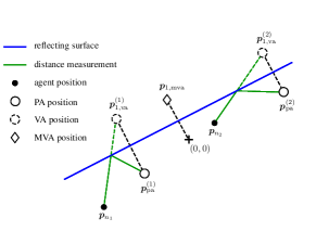
Figure 1: A graphical depiction of a multipath-based localization scenario involving $K=1$ reflective surfaces, $J=2$ PAs, and positions of the agent $\bm{p}_{n}$ at two time steps $n\in\{n_{1},n_{2}\}$.

By using some algebra, the transformation from MVA $\bm{p}_{k,\mathrm{mva}}$ to VA position $\bm{p}^{(j)}_{\mathrm{pa}}$ can be obtained as

$$\bm{p}^{(j)}_{k,\mathrm{va}} =-\bigg{(}\frac{2\big{\langle}\bm{p}_{k,\mathrm{mva}},\bm{p}^{(j)}_{\mathrm{pa}}\big{\rangle}}{\big{\|}\bm{p}_{k,\mathrm{mva}}\big{\|}^{2}}-1\bigg{)}\hskip 0.85358pt\bm{p}_{k,\mathrm{mva}}+\hskip 0.85358pt\bm{p}^{(j)}_{\mathrm{pa}}$$

$$=h\big{(}\bm{p}_{k,\mathrm{mva}},\bm{p}^{(j)}_{\mathrm{pa}}\big{)}.$$ (1)

where $\langle\cdot,\cdot\rangle$ represents the inner-product between two vectors.

Based on the nonlinear transformation in (1), the distance measurement related to the propagation path agent – surface $k$ – PA $j$ can now alternatively be expressed by [12]

$$z_{m,n}^{(j)} =\big{\|}\bm{p}_{n}-h\big{(}\bm{p}_{k,\mathrm{mva}},\bm{p}^{(j)}_{\mathrm{pa}}\big{)}\big{\|}+\nu_{m,n}^{(j)}.$$ (2)

Using (2) as well as the known PA position $\bm{p}^{(j)}_{\mathrm{pa}}$, we can directly obtain the MVA-based likelihood function as $f\big{(}z_{m,n}^{(j)}\big{|}\bm{p}_{k,\mathrm{mva}},\bm{p}_{n}\big{)}\vspace{.8mm}$. Note that with the proposed MVA-based measurement model, at time $n$, the measurements collected by all PAs $j=1,\ldots,J$ can provide information on the same MVA and agent positions $\bm{p}_{k,\mathrm{mva}},k\in\{1,\dots,K\}$ and $\bm{p}_{n}$, respectively. The number of MVAs $K$ is unknown. As an example, Fig. 1 shows a scenario with two PAs $j\in\{1,2\}$ and two time steps $n_{1}$ and $n_{2}$. Note that due to measurement origin uncertainty there is an unknown association of measurements with MVAs. Furthermore there can be missed detections, i.e., at some time steps $n$ actual MVAs may not produce a measurement at some PA $j$; and false alarms, i.e., there may be clutter measurements not generated by any MVA (see [3, 8, 4, 10] for details).

At each time $n$, the state of the agent $\bm{x}_{n}$ consists of it’s position $\bm{p}_{n}$ and possibly further motion related parameters. As in [14, 15, 3], we account for the unknown number of MVAs by introducing potential s $k\in\{1,\dots,K_{n}\}$. The number $K_{n}$ of PMVAs is the maximum possible number of actual MVA that produced a measurement so far [15] (where $K_{n}$ increases with time). PMVA states are denoted as $\bm{y}_{k,n}=\big{[}\bm{p}^{\text{T}}_{k,\mathrm{mva}}\;r_{k,n}\big{]}^{\text{T}}$. The existence/nonexistence of PMVA $k$ is modeled by the existence variable $r_{k,n}\in\{0,1\}$ in the sense that PMVA $k$ exists if and only if $r_{k,n}\!=\!1$. It is considered formally also if PMVA $k$ is nonexistent, i.e., if $r_{k,n}\!=0$. The states $\bm{p}^{\text{T}}_{k,\mathrm{mva}}$ of nonexistent PMVAs are obviously irrelevant. Therefore, all PDFs defined for PMVA states, $f(\bm{y}_{k,n})=f(\bm{p}_{k,\mathrm{mva}},r_{k,n})$, are of the form $f(\bm{p}_{k,\mathrm{mva}},0)$ $=f_{k,n}f_{\text{d}}(\bm{p}_{k,\mathrm{mva}})$, where $f_{\text{d}}(\bm{p}_{k,\mathrm{mva}})$ is an arbitrary “dummy PDF” and $f_{k,n}\!\in[0,1]$ is a constant. Further details for the system model of MVA-based RF-SLAM are provided in [12].

III Problem Formulation and Proposed Method

We aim to estimate the agent state $\bm{x}_{n}$ using all available measurements $\bm{z}_{1:n}$ from all PAs up to time $n$. In particular, we calculate an estimate $\hat{\bm{x}}_{n}$ by using the minimum mean-square error (MMSE) estimator [16, Ch. 4]

$$\hat{\bm{x}}_{n}\hskip 0.85358pt\triangleq\,\int\bm{x}_{n}\hskip 0.85358ptf(\bm{x}_{n}|\bm{z}_{1:n})\hskip 0.85358pt\mathrm{d}\bm{x}_{n}.\vspace{.5mm}$$ (3)

For the mapping of reflection surfaces, detection of PMVAs $k\!\in\!\{1,\dots,K_{n}\}$ and estimation their positions $\bm{p}_{k,\mathrm{mva}}$ is considered. This relies on the marginal posterior existence probabilities $p(r_{k,n}\!=\!1|\bm{z}_{1:n})$ and the marginal posterior PDFs $f(\bm{x}_{k,n}|r_{k,n}\!=\!1,\bm{z}_{1:n})$. A PMVA $k$ is declared to exist if $p(r_{k,n}\!=\!1|\bm{z}_{1:n})>p_{\text{de}}$, where $p_{\text{de}}$ is a detection threshold [16, Ch. 2]. The number $\hat{K}_{n}$ of PMVA states that are considered to exist is the estimate of total number $K$ of MVAs. For existing PMVAs, an estimate of it’s position $\bm{p}_{k,\mathrm{mva}}$ can again be calculated by the MMSE [16, Ch. 4]

$$\hat{\bm{p}}_{k,\mathrm{mva}}\,\triangleq\int\bm{p}_{k,\mathrm{mva}}\hskip 0.85358pt\hskip 0.85358ptf(\bm{p}_{k,\mathrm{mva}}\hskip 0.85358pt|\hskip 0.85358ptr_{k,n}\!=\!1,\bm{z}_{1:n})\hskip 0.85358pt\hskip 0.85358pt\mathrm{d}\bm{p}_{k,\mathrm{mva}}.\vspace{.5mm}$$ (4)

The calculation of $f(\bm{x}_{n}|\bm{z}_{1:n})$, $p(r_{k,n}\!=\!1|\bm{z})$, and $f(\bm{p}_{k,\mathrm{mva}}|$ $r_{k,n}=1,\bm{z}_{1:n})$ from the joint posterior PDF [12, Eq. (4)] by direct marginalization is not feasible.

By performing sequential sample-based message passing by means of the SPA rules [17, 18, 14, 3] on the factor graph in [12, Fig. 3], approximations (“beliefs”) of the marginal posterior PDFs $q(\bm{x}_{n})\approx f(\bm{x}_{n}|\bm{z}_{1:n})$ and $q(\bm{p}_{k,\mathrm{mva}},r_{k,n})\approx f(\bm{p}_{k,\mathrm{mva}},r_{k,n}|\bm{z}_{1:n})$, $k\in\{1,\dots,K_{n}\}$ can be obtained in an efficient ways. More specifically, representations of beliefs that consist of $I$ weighted random samples or particles denoted as $\big{\{}\bm{x}^{(i)}_{n},\mathpzc{w}_{n}^{(i)}\big{\}}^{I}_{i=1}\sim q(\bm{x}_{n})$ and $\big{\{}\big{(}\bm{p}^{(i)}_{k,\mathrm{mva}},w_{k,n}^{(i)}\big{)}\big{\}}^{I}_{i=1}\sim q(\bm{p}_{k,\mathrm{mva}},r_{k,n})$, $k\in\{1,\dots,K_{n}\}$ are computed [18, 14, 3]. Note that $\sum^{I}_{i=1}\mathpzc{w}_{n}^{(i)}=1$ while $\sum^{I}_{i=1}w_{k,n}^{(i)}\approx p(r_{k,n}\!=\!1|\bm{z})$ (cf. [14, Sec. VI]). These sample-based representations can be used for approximate MMSE estimation by evaluating (3) and (4) based on Monte Carlo integration [19]. To avoid the number of PMVA states growing indefinitely, PMVAs states with $p(r_{k,n}=1\hskip 0.85358pt|\hskip 0.85358pt\bm{z}_{1:n})$ below a threshold $p_{\text{pr}}$ are removed from the state space (“pruned”). Pruning is performed at each time $n$, after the measurements of all PAs have been processed.

IV Review of Bootstrap Sampling for RF-SLAM

Existing RF-SLAM methods employ the bootstrap sampling strategy [11] where predicted beliefs are employed as proposal PDF. In particular, the proposal distribution for calculating the belief $q(\bm{p}_{k,\mathrm{mva}},r_{k,n})$ of MVA, $k\in\{1,\dots,K_{n}\}$ at time $n$ is given by (cf. [18, 3, 12])

$$f_{\mathrm{pred.}}(\bm{x}_{n},\bm{p}_{k,\mathrm{mva}})\propto\alpha(\bm{p}_{k,\mathrm{mva}},r_{k,n}=1)\hskip 0.85358pt\alpha(\bm{x}_{n})$$ (5)

where $\propto$ indicates equality up to a normalization factor and the “prediction messages” $\alpha(\bm{p}_{k,\mathrm{mva}},r_{k,n})$ and $\alpha(\bm{x}_{n})$ can be obtained as

$$\alpha(\bm{x}_{n}) =\int f(\bm{x}_{n}|\bm{x}_{n-1})\hskip 0.85358ptq(\bm{x}_{n-1})\hskip 0.85358pt\mathrm{d}\bm{x}_{n-1}$$

$$\alpha(\bm{p}_{k,\mathrm{mva}},r_{k,n}) =\sum_{r_{k,n-1}\in\{0,1\}}\int f\big{(}\bm{p}_{k,\mathrm{mva}}\hskip 0.85358pt,r_{k,n}\hskip 0.85358pt\big{|}\hskip 0.85358pt\bm{p}_{k,\mathrm{mva}}\hskip 0.85358pt,r_{k,n-1}\big{)}$$

$$\hskip 42.67912pt\times q\big{(}\bm{p}_{k,\mathrm{mva}},r_{k,n-1}\big{)}\hskip 0.85358pt\mathrm{d}\bm{p}_{k,\mathrm{mva}}\hskip 0.85358pt.\vspace{-1.2mm}$$ (6)

Here, $f(\bm{x}_{n}|\bm{x}_{n-1})$ and $f\big{(}\bm{p}_{k,\mathrm{mva}}\hskip 0.85358pt,r_{k,n}\hskip 0.85358pt\big{|}\hskip 0.85358pt\bm{p}_{k,\mathrm{mva}}\hskip 0.85358pt,r_{k,n-1}\big{)}$ are the state-transition functions for the agent state and the MVA state, respectively [12, Sec. II]. Furthermore, the beliefs of the agent state, $q(\bm{x}_{n-1})$, and of the MVA states $q\big{(}\bm{p}_{k,\mathrm{mva}},r_{k,n-1}\big{)}$, were calculated at the preceding time $n-\!1$. Note that for the proposal $f_{\mathrm{pred.}}(\bm{x}_{n},\bm{p}_{k,\mathrm{mva}})$ in (5), we only use the functional form of $\alpha(\bm{p}_{k,\mathrm{mva}},r_{k,n})$ for the case $r_{k,n}=1$, since the functional form for the case $r_{k,n}=0$ is always equal to the dummy PDF $f_{\text{d}}(\bm{p}_{k,\mathrm{mva}})$. Samples of $f_{\mathrm{pred.}}(\bm{x}_{n},\bm{p}_{k,\mathrm{mva}})$ can be obtained as discussed in [14, 3].

The proposal distribution in (5) has to be a function of both MVA position $\bm{p}_{k,\mathrm{mva}}$ and agent state $\bm{x}_{n}$, since the measurement model (2) also involves both MVA state and agent state. Furthermore, note that the proposal distribution in (5) is also used to calculate a factor that represents the contribution of MVA $k\in\{1,\dots,K_{n}\}$ to the agent weights $\mathpzc{w}_{n}^{(i)}$, $i\in\{1,\dots,I\}$ (cf. [18, 3, 12]).

Bootstrap sampling is suitable for RF-SLAM methods that consider VAs as the features to be mapped [3, 8, 4]. However, its use for the fast and more accurate MVAs-based RF-SLAM is problematic in challenging RF-SLAM scenarios with one or two PAs where only range measurements are available. This is because, due to certain geometric symmetries, for some initial time steps after an MVA has been introduced, the PDFs of an MVA can be multi-modal. In addition, during these initial time steps, often, the dominant mode might not be the one located at the correct MVA position. Thus, the sample representations provided by bootstrap sampling may collapse in a wrong mode, i.e., converge to incorrect MVA positions corresponding to local maxima.

V Robust Sampling for MVA-based RF-SLAM

To address these limitations, we introduce an alternative strategy for obtaining a proposal distribution. In what follows, we will again discuss the proposal distribution for the belief $q(\bm{p}_{k,\mathrm{mva}},r_{k,n})$ of MVA, $k\in\{1,\dots,K_{n}\}$. As discussed later this proposal will just be used at certain time steps $n$.

The main idea is to construct a weighted mixture that consists of MVA position information that is predicted and MVA position information that is related to the best measurement for each PA $j=1,\ldots,J$ obtained at time step $n-1$. A measurement is the best if it has the largest probability of association with MVA $k$ at time $n-1$. The index of this best measurement is denoted by $m^{(j)}_{k,n-1}\in\big{\{}0,1,\dots,M^{(j)}_{n-1}\big{\}}$, where $m^{(j)}_{k,n-1}=0$ indicates that no measurement is the best, i.e., the probability of no measurement being associated to the MVA (“missed detection”) is larger than the probability of association with any measurement. To construct the proposal distribution at time $n$, we use the measurements from time $n-1$ because association probabilities at time $n-1$ have already been calculated [3]; on the other hand, calculation of association probabilities at time $n$ is based on the proposal distribution at time $n$.

The considered proposal distribution at time $n$, is given by

$$f_{\mathrm{mixture}}(\bm{x}_{n},\bm{p}_{k,\mathrm{mva}})$$

$$\hskip 17.07164pt\triangleq f_{\mathrm{pred.}}(\bm{x}_{n},\bm{p}_{k,\mathrm{mva}})+\sum_{j\in{\cal{J}}}f^{(j)}_{\mathrm{meas.}}(\bm{x}_{n},\bm{p}_{k,\mathrm{mva}})$$ (7)

where ${\cal{J}}$ consists of all indexes $j$ with $m^{(j)}_{k,n-1}\neq 0$. Furthermore, the component related to the best measurements reads

$$f^{(j)}_{\mathrm{meas.}}(\bm{x}_{n},\bm{p}_{k,\mathrm{mva}})\propto\alpha(\bm{x}_{n})f\big{(}z_{m^{(j)}_{k,n-1},n-1}^{(j)}\big{|}\bm{p}_{k,\mathrm{mva}},\bm{p}_{n}\big{)}.$$

Samples of $f^{(j)}_{\mathrm{meas.}}(\bm{x}_{n},\bm{p}_{k,\mathrm{mva}})$ can be obtained by following the importance sampling principle [19]. In particular, samples $\big{\{}(\tilde{\bm{x}}^{(i)}_{n},\tilde{\bm{p}}^{(i)}_{k,\mathrm{mva}})\big{\}}^{I^{\prime}}_{i=1}$ are drawn from $\alpha(\bm{x}_{n})\hskip 0.85358ptf_{\mathrm{uni.}}(\bm{p}_{k,\mathrm{mva}})$ first, where $f_{\mathrm{uni.}}(\bm{p}_{k,\mathrm{mva}})$ is a PDF that is uniform on the area of interest. Then corresponding unnormalized weights are calculated as

$$\tilde{w}^{(i)}_{k,n}=\frac{f\Big{(}z_{m^{(j)}_{k,n-1},n-1}^{(j)}\hskip 0.85358pt\big{|}\hskip 0.85358pt\tilde{\bm{p}}^{(i)}_{k,\mathrm{mva}},\tilde{\bm{p}}^{(i)}_{n}\Big{)}}{f_{\mathrm{uni.}}\big{(}\tilde{\bm{p}}^{(i)}_{k,\mathrm{mva}}\big{)}}.$$ (8)

The samples $\big{\{}(\bm{x}^{(i)}_{n},\bm{p}^{(i)}_{k,\mathrm{mva}})\big{\}}^{I^{\prime}}_{i=1}$ representing $f^{(j)}_{\mathrm{meas.}}(\bm{x}_{n},$ $\bm{p}_{k,\mathrm{mva}})$ are computed from $\big{\{}(\tilde{\bm{x}}^{(i)}_{n},\tilde{\bm{p}}^{(i)}_{k,\mathrm{mva}},\tilde{w}^{(i)}_{k,n})\big{\}}^{I^{\prime}}_{i=1}$ by first normalizing the weights $\tilde{w}^{(i)}_{k,n}$, $i\in\{1,\dots,I^{\prime}\}$ and then performing a resampling step [19]. Finally, $I$ samples of the considered proposal distribution $f_{\mathrm{mixture}}(\bm{x}_{n},\bm{p}_{k,\mathrm{mva}},r_{k,n})$ in (7) are obtained as follows: (i) $I^{\prime}$ is selected as small as possible such that $I^{\prime}(|{\cal{J}}|+1)\geqslant I$; (ii) $I^{\prime}$ samples from $f_{\mathrm{pred.}}(\bm{x}_{n},\bm{p}_{k,\mathrm{mva}})$ and from each $f^{(j)}_{\mathrm{meas.}}(\bm{x}_{n},\bm{p}_{k,\mathrm{mva}})$, $j\in{\cal{J}}$, are obtained; and (iii) $I$ of the resulting $I^{\prime}(|{\cal{J}}|+1)$ samples are selected randomly.

The main advantage of using (7) as the proposal distribution is that particles are again spread out over a wider area of potential MVA locations and thus collapsing to a wrong mode is avoided. On the other hand, using (7) at each time step would significantly reduce the speed of convergence to the correct mode. In our numerical evaluation of MVA-based RF-SLAM, we found it useful to only use the proposal distribution (7) at certain time steps $n^{\prime}$ that are determined randomly. Let $n_{1}$ be the last time steps where (7) has been used. The next time step $n_{2}$ where (7) is used can now be obtained by sampling from the uniform probability mass function (PMF) $p_{\mathrm{uni.}}\big{(}n_{2};n_{1}+N_{\mathrm{1}},n_{1}+N_{\mathrm{2}}\big{)}$. Finally, the proposal (7) is not used anymore after the PMVA has existed for a certain number of time steps $N_{\mathrm{max}}$. A possible choice for the hyperparameters $N_{\mathrm{1}}$, $N_{\mathrm{2}}$ are $N_{\mathrm{max}}$ is discussed in Section VI. When we calculate the weights of the samples drawn from the proposal (7), we perform an approximation and avoid the costly evaluation of (7). As demonstrated in Section VI, despite this approximation the proposed robust sampling can yield convincing MVA-based RF-SLAM performance.

VI Simulation Results

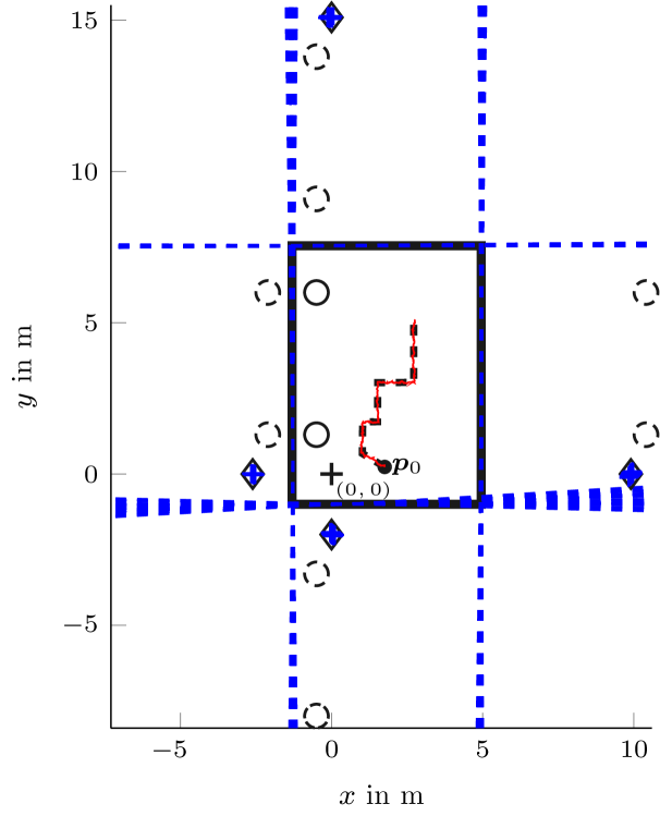
Figure 2: Considered scenario for performance evaluation with three PAs, four reflective surfaces and corresponding MVAs and VAs, as well as agent trajectory.

The proposed robust sampling for MVA-based RF-SLAM is validated in the indoor scenario shown in Figure 2. The scenario consists of four reflective surfaces, i.e., $K=4$ MVAs, as well as two PAs at positions $\bm{p}_{\mathrm{pa}}^{(1)}=[-0.5\hskip 2.84526pt\hskip 2.84526pt6]^{\text{T}}$ and $\bm{p}_{\mathrm{pa}}^{(3)}=[-0.5\hskip 2.84526pt\hskip 2.84526pt1.3]^{\text{T}}$. We compare the proposed method with MVA-based RF-SLAM that relies on bootstrap sampling [12].

The agent’s state-transition PDF $f(\bm{x}_{n}|\bm{x}_{n-1})$, with $\bm{x}_{n}=[\bm{p}_{n}^{\text{T}}\;\bm{v}_{n}^{\text{T}}]^{\text{T}}$, is defined by a linear, near constant-velocity motion model [20, Sec. 6.3.2], i.e., $\bm{x}_{n}=\bm{A}\bm{x}_{n-1}+\bm{B}\bm{\omega}_{n}$. Here, $\bm{A}\in\mathbb{R}^{4\times 4}$ and $\bm{B}\in\mathbb{R}^{4\times 2}$ are as defined in [20, Sec. 6.3.2] (with sampling period $\Delta T=1\,\text{s}$), and the driving process $\bm{\omega}_{n}$ is iid across $n$, zero-mean, and Gaussian with covariance matrix $\sigma_{\omega}^{2}\mathbb{I}_{2}$, where $\mathbb{I}_{2}$ denotes the $2\times 2$ identity matrix and $\sigma_{\omega}=0.0032\,\text{m}/\text{s}^{2}$. For the sake of numerical stability, we introduced a small regularization noise to the PMVA state $\bm{p}_{k,\mathrm{mva}}$ at each time $n$, i.e., $\underline{\bm{p}}_{k,\mathrm{mva}}=\bm{p}_{k,\mathrm{mva}}+\bm{a}_{k}$, where $\bm{a}_{k}$ is iid across $k$, zero-mean, and Gaussian with covariance matrix $\sigma_{\bm{a}}^{2}\mathbb{I}_{2}$ and $\sigma_{\bm{a}}=10^{-5}\,\text{m}$.

We performed 300 simulation runs using 30,000 samples, each using the floor plan and agent trajectory shown in Fig. 2. In each simulation run, we generated noisy distance measurements $z_{m,n}^{(j)}$ according to (2) with noise standard deviation $\sigma_{m,n}^{(j)}=0.1\,$m and detection probability $p_{\mathrm{d}}=0.95$. In addition, a mean number $\mu_{\mathrm{fa}}=1$ of false alarm measurements $z_{m,n}^{(j)}$ were generated according to a false alarm PDF $f_{\mathrm{fa}}(z_{m,n}^{(j)})$ that is uniform on $[0\,\text{m}\hskip 0.85358pt\hskip 0.85358pt\hskip 0.85358pt30\,\text{m}]$. The samples for the initial agent state are drawn from a 4-D uniform distribution with center $\bm{x}_{0}=[\bm{p}_{0}^{\text{T}}\;0\;\,0]^{\text{T}}$, where $\bm{p}_{0}$ is the starting position of the actual agent trajectory. The support of each position component about the respective center is given by $[-0.1\,\text{m},0.1\,\text{m}]$ and of each velocity component is given by $[-0.01\,\text{m/s},0.01\,\text{m/s}]$. At time $n=0$, the number of MVAs is $K_{0}=0$, i.e., no prior map information is available. The prior distribution for new PMVA states $f_{\mathrm{n}}(\overline{\bm{y}}_{m,n})$ is uniform on the square region given by $[-15\,\text{m},\hskip 0.85358pt15\,\text{m}]\hskip 0.85358pt\times\hskip 0.85358pt[-15\,\text{m},\hskip 0.85358pt15\,\text{m}]$ around the center of the floor plan shown in Fig. 2 and the mean number of new PMVA at time $n$ is $\mu_{n}=0.01$. The probability of survival is $p_{\mathrm{s}}=0.999$, the detection threshold is $p_{\mathrm{de}}=0.5$, and the pruning threshold is $p_{\mathrm{pr}}=10^{-3}$. The parameters for robust sampling are $N_{1}=5$, $N_{2}=10$, and $N_{\text{max}}=120$, respectively.

(a)

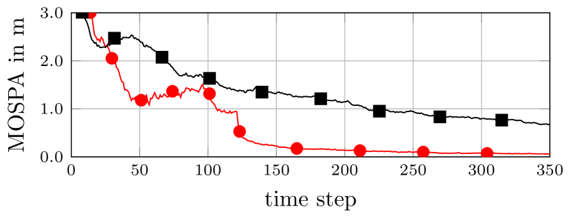
(b)

Figure 3: Preliminary performance results: (a) RMSE position errors of the MVAs and (b) RMSE of the mobile agent.

As an example, Fig. 2 depicts for one simulation run the posterior PDFs represented by samples of the MVA positions and corresponding reflective surfaces as well as estimated agent tracks. Fig. 3a shows the mean optimal subpattern assignment (MOSPA) errors [21] of the MVA positions, all versus time $n$. The MOSPA errors are based on the Euclidean metric with cutoff parameter $c=5\,$m and order $p=1$. The red line shows the MOSPA errors of the proposed MVA-based SLAM algorithm and the black line shows the MOSPA errors of the algorithm presented in [12]. The MOSPA error of the proposed MVA-based SLAM algorithm converges to a much smaller mapping error than that of the algorithm presented in [12]. This can be explained by the symmetric multi-modality of the marginal posterior PDFs. The proposed robust sampling avoids the behavior where all samples collapse into the wrong mode. However, since the robust sampling “excites” the multi-modality of the marginal PDF of the MVAs, the MOSPA error remains quite large until robust sampling is disabled at time $n=120$. Finally, Fig. 3b shows the RMSEs of the agent positions of the converged simulation runs versus time $n$. We define a simulation run to be converged if $\{\forall n:||\hat{\bm{x}}_{n}-\bm{x}_{n}||<0.5\}$. For the converged runs both methods have an agent RMSE below $0.1\,$m, however, the agent RMSE provided by the proposed algorithms is still significantly smaller. More importantly, only one of the $300$ simulation runs diverged for the proposed algorithm, but $38\,$% of the simulation runs diverged for the algorithm in [12].

VII Conclusions and Future Work

In this paper, we introduced MVA-based RF-SLAM with an improved sampling technique that is suitable for challenging scenarios where only range measurements are available, and only one or two PAs are deployed. Our numerical evaluation demonstrated significant performance advantages of the proposed method compared to the recently introduced conventional MVA-based RF-SLAM. Promising directions for future research are an extension of MVA-based RF-SLAM to (i) angle measurements provided by antenna arrays and (ii) higher-order reflections from flat surfaces.

References

- [1] K. Witrisal, P. Meissner, E. Leitinger, Y. Shen, C. Gustafson, F. Tufvesson, K. Haneda, D. Dardari, A. F. Molisch, A. Conti, and M. Z. Win, “High-accuracy localization for assisted living,” IEEE Signal Process. Mag., vol. 33, no. 2, pp. 59–70, Mar. 2016.
- [2] C. Gentner, T. Jost, W. Wang, S. Zhang, A. Dammann, and U. C. Fiebig, “Multipath assisted positioning with simultaneous localization and mapping,” IEEE Trans. Wireless Commun., vol. 15, no. 9, pp. 6104–6117, Sep. 2016.
- [3] E. Leitinger, F. Meyer, F. Hlawatsch, K. Witrisal, F. Tufvesson, and M. Z. Win, “A Belief Propagation Algorithm for Multipath-Based SLAM,” IEEE Trans. Wireless Commun., vol. 18, no. 11, Dec. 2019.
- [4] R. Mendrzik, F. Meyer, G. Bauch, and M. Z. Win, “Enabling situational awareness in millimeter wave massive MIMO systems,” IEEE J. Sel. Topics Signal Process., vol. 13, no. 5, pp. 1196–1211, Sep. 2019.
- [5] H. Durrant-Whyte and T. Bailey, “Simultaneous localization and mapping: Part I,” IEEE Robot. Autom. Mag., vol. 13, no. 2, pp. 99–110, Jun. 2006.
- [6] M. Dissanayake, P. Newman, S. Clark, H. Durrant-Whyte, and M. Csorba, “A solution to the simultaneous localization and map building (SLAM) problem,” IEEE Trans. Robot. Autom., vol. 17, no. 3, pp. 229–241, Jun. 2001.
- [7] J. Mullane, B.-N. Vo, M. Adams, and B.-T. Vo, “A random-finite-set approach to Bayesian SLAM,” IEEE Trans. Robot., vol. 27, no. 2, pp. 268–282, Apr. 2011.
- [8] E. Leitinger, S. Grebien, and K. Witrisal, “Multipath-based SLAM exploiting AoA and amplitude information,” in Proc. IEEE ICCW-19, Shanghai, China, May 2019, pp. 1–7.
- [9] F. Meyer and K. L. Gemba, “Probabilistic focalization for shallow water localization,” J. Acoust. Soc, vol. 150, no. 2, pp. 1057–1066, 2021.
- [10] F. Meyer and J. L. Williams, “Scalable detection and tracking of geometric extended objects,” IEEE Trans. Signal Process., vol. 69, pp. 6283–6298, 2021.
- [11] M. S. Arulampalam, S. Maskell, N. Gordon, and T. Clapp, “A tutorial on particle filters for online nonlinear/non-Gaussian Bayesian tracking,” IEEE Trans. Signal Process., vol. 50, no. 2, pp. 174–188, Feb. 2002.
- [12] E. Leitinger and F. Meyer, “Data fusion for multipath-based SLAM,” in Proc. Asilomar-20, Pacifc Grove, CA, USA, Oct. 2020, pp. 934–939.
- [13] M. A. Badiu, T. L. Hansen, and B. H. Fleury, “Variational Bayesian inference of line spectra,” IEEE Trans. Signal Process., vol. 65, no. 9, pp. 2247–2261, May 2017.
- [14] F. Meyer, P. Braca, P. Willett, and F. Hlawatsch, “A scalable algorithm for tracking an unknown number of targets using multiple sensors,” IEEE Trans. Signal Process., vol. 65, no. 13, pp. 3478–3493, Jul. 2017.
- [15] F. Meyer, T. Kropfreiter, J. L. Williams, R. A. Lau, F. Hlawatsch, P. Braca, and M. Z. Win, “Message passing algorithms for scalable multitarget tracking,” Proc. IEEE, vol. 106, no. 2, pp. 221–259, Feb. 2018.
- [16] H. V. Poor, An Introduction to Signal Detection and Estimation, 2nd ed. New York: Springer-Verlag, 1994.
- [17] F. R. Kschischang, B. J. Frey, and H.-A. Loeliger, “Factor graphs and the sum-product algorithm,” IEEE Trans. Inf. Theory, vol. 47, no. 2, pp. 498–519, Feb. 2001.
- [18] F. Meyer, O. Hlinka, H. Wymeersch, E. Riegler, and F. Hlawatsch, “Distributed localization and tracking of mobile networks including noncooperative objects,” IEEE Trans. Signal Inf. Process. Netw., vol. 2, no. 1, pp. 57–71, Mar. 2016.
- [19] A. Doucet, N. de Freitas, and N. Gordon, Sequential Monte Carlo Methods in Practice. New York, NY: Springer, 2001.
- [20] Y. Bar-Shalom, T. Kirubarajan, and X.-R. Li, Estimation with Applications to Tracking and Navigation. New York, NY, USA: Wiley, 2002.
- [21] D. Schuhmacher, B.-T. Vo, and B.-N. Vo, “A consistent metric for performance evaluation of multi-object filters,” IEEE Trans. Signal Process., vol. 56, no. 8, pp. 3447–3457, Aug. 2008.