Guided Safe Shooting: model based reinforcement learning with safety constraints

Abstract

In the last decade, reinforcement learning successfully solved complex control tasks and decision-making problems, like the Go board game. Yet, there are few success stories when it comes to deploying those algorithms to real-world scenarios. One of the reasons is the lack of guarantees when dealing with and avoiding unsafe states, a fundamental requirement in critical control engineering systems. In this paper, we introduce Guided Safe Shooting (GuSS), a model-based RL approach that can learn to control systems with minimal violations of the safety constraints. The model is learned on the data collected during the operation of the system in an iterated batch fashion, and is then used to plan for the best action to perform at each time step. We propose three different safe planners, one based on a simple random shooting strategy and two based on MAP-Elites, a more advanced divergent-search algorithm. Experiments show that these planners help the learning agent avoid unsafe situations while maximally exploring the state space, a necessary aspect when learning an accurate model of the system. Furthermore, compared to model-free approaches, learning a model allows GuSS reducing the number of interactions with the real-system while still reaching high rewards, a fundamental requirement when handling engineering systems.

1 Introduction

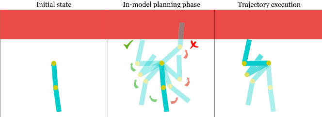
Figure 1: An illustrative example of planning with model-based approach on the Acrobot environment. The agent controls the torque on the first joint with the goal of getting its end effector as high as possible, avoiding the unsafe zone (red area). Starting in the rest position (left) the agent uses its model to find the best plan (middle) that will maximize the reward while satisfying the safety constraint and execute it on the real system (right). The example is especially relevant to applications in which safety and reward are traded off.

In recent years, deep Reinforcement Learning (RL) solved complex sequential decision-making problems in a variety of domains, such as controlling robots, and video and board games [23, 4, 32]. However, in the majority of these cases, success is limited to a simulated world. The application of these RL solutions to real-world systems is still yet to come. The main reason for this gap is the fundamental principle of RL of learning by trial and error to maximize a reward signal [34]. This framework requires unlimited access to the system to explore and perform actions possibly leading to undesired outcomes. This is not always possible, for example, considering the task of finding the optimal control strategy for a data center cooling problem [17], the RL algorithm could easily take actions leading to high temperatures during the learning process, affecting and potentially breaking the system. Another domain where safety is crucial is robotics. Here unsafe actions could not only break the robot but could potentially also harm humans. This issue, known as safe exploration, is a central problem in AI safety [3]. This is why most achievements in RL are in simulated environments, where the agents can explore different behaviors without the risk of damaging the real system. However, those simulators are not always accurate enough, if available at all, leading to suboptimal control strategies when deployed on the real-system [30].

With the long-term goal of deploying RL algorithms on real engineering systems, it is imperative to overcome those limitations. A straightforward way to address this issue is to develop algorithms that can be deployed directly on the real system that provide guarantees in terms of constraints, such as safety, to ensure the integrity of the system. This could potentially have a great impact, as many industrial systems require complex decision-making, which efficient RL systems can easily provide. Going towards this goal, in this paper we introduce Guided Safe Shooting (GuSS), a safe Model Based Reinforcement Learning (MBRL) algorithm that learns a model of the system and uses it to plan for a safe course of actions through Model Predictive Control (MPC) [12]. GuSS learns the model in an iterated batch fashion [22, 14], allowing for minimal real-system interactions. This is a desirable property for safe RL approaches, as fewer interactions with the real-system mean less chance of entering unsafe states, a condition difficult to attain with model-free safe RL methods [1, 29, 35]. Moreover, by learning a model of the system, this allows flexibility and safety guarantees as using the model we can anticipate unsafe actions before they occur. Consider the illustrative example in Fig. 1: the agent, thanks to the model of its dynamics, can perform “mental simulation” and select the best plan to attain its goal while avoiding unsafe zones. This contrasts with many of the methods in the literature that address the problem of finding a safe course of action through Lagrangian optimization or by penalizing the reward function [36, 21, 9]. GuSS avoids unsafe situations by discarding trajectories that are deemed unsafe using the model predictions. Within this framework, we propose three different safe planners, one based on a simple random shooting strategy and two based on MAP-Elites (ME) [25], a more advanced divergent-search algorithm. These planners are used to generate, evaluate, and select the safest actions with the highest rewards. Using divergent-search methods for planning allows the agent to more widely explore the possible courses of actions. This leads to both a safer and more efficient search, while covering a higher portion of the state space, an important factor when learning a model, given that more exploratory datasets lead to better models [40].

Experiments conducted on two different environments show that GuSS can efficiently deal with sensitive systems, avoiding unsafe states while learning a good model of the system. The presented results highlight how the model and planners can easily find strategies reaching high rewards with minimal costs, even when the two metrics are antithetical, as is the case for the Safe Acrobot environment.

To recap, the contributions of the paper are the following:

• We introduce Guided Safe Shooting (GuSS), an MBRL method capable of efficiently learning to avoid unsafe states while optimizing the reward, outperforming both model-free and other model-based safe approaches;

• We propose the use of divergent-search methods as MAP-Elites (ME) as planning techniques in MBRL approaches;

• We present 3 different planners, Safe Random Shooting (S-RS), Safe MAP-Elites (S-ME), Pareto Safe MAP-Elites (PS-ME), that can generate a wide array of action sequences while discarding the ones deemed unsafe during planning.

2 Related Work

Some of the most common techniques addressing safety in RL rely on solving a Constrained Markov Decision Process (CMDP) [2] through model-free RL methods [1, 29, 35, 13, 41]. Among these approaches, a well-known method is CPO [1] which adds constraints to the policy optimization process in a fashion similar to TRPO [31]. A similar approach is taken by PCPO [39] and its extension [38]. The algorithm works by first optimizing the policy with respect to the reward and then projecting it back on the constraint set in an iterated two-step process. A different strategy consists in storing all the “recovery” actions that the agent took to leave unsafe regions in a separate replay buffer [13]. This buffer is used whenever the agent enters an unsafe state by selecting the most similar transition in the safe replay buffer and performing the same action to escape the unsafe state.

Model-free RL methods need many interactions with the real-system in order to collect the data necessary for training. This can be a huge limitation in situations in which safety is critical, where increasing the number of samples increases the probability of entering unsafe states. MBRL limits this problem by learning a model of the system that can then be used to learn a safe policy. This allows increased flexibility in dealing with unsafe situations, even more if the safety constraints change in time.

Many of these methods work by modifying either the cost or the reward function to push the algorithm away from unsafe areas. The authors of uncertainty guided Cross-Entropy Methods (CEM) [36] extend PETS [8] by modifying the objective function of the CEM-based planner to avoid unsafe areas. In this setting, an unsafe area is defined as the set of states for which the ensemble of models has the highest uncertainty. A different strategy is to inflate the cost function with an uncertainty-aware penalty function, as done in CAP [21]. This cost change can be applied to any MBRL algorithm and its conservativeness is automatically tuned through the use of a PI controller. Another approach, SAMBA [9], uses Gaussian Processes (GP) to model the environment. This model is then used to train a policy by including the safety constraint in the optimization process through Lagrangian multipliers. Closer to GuSS are other methods using a trajectory sampling approach to select the safest trajectories generated by CEM [37, 19]. This lets us deal with the possible uncertainties of the model predictions that could lead to consider a trajectory safe when it is not.

3 Background

In this section, we introduce the basic concepts of safe-RL and divergent-search algorithms, on which our method builds.

3.1 Safe Reinforcement Learning

Reinforcement learning problems are usually represented as a Markov decision process (MDP) $\mathcal{M}=\langle\mathcal{S},\mathcal{A},\mathcal{T},r,\gamma\rangle$, where $\mathcal{S}$ is the state space, $\mathcal{A}$ is the action space, $\mathcal{T}:\mathcal{S}\times\mathcal{A}\rightarrow\mathcal{S}$ is the transition dynamics, $r:\mathcal{S}\times\mathcal{A}\rightarrow\mathbb{R}$ is the reward function and $\gamma\in[0,1]$ is the discount factor. Let $\Delta(\mathcal{X})$ denote the family of distributions over a set $\mathcal{X}$. The goal is to find a policy $\pi:\mathcal{S}\rightarrow\Delta(\mathcal{A})$ which maximizes the expected discounted return $\pi^{*}=\underset{\pi}{\arg\max}$ $\mathbb{E}_{\pi}\left[\sum_{t}\gamma^{t}r(s_{t},a_{t})\right]$ [34]. This formulation can be easily accommodated to incorporate constraints, for example representing safety requirements. To do so, similarly to the reward function, we define a new cost function $\mathcal{C}:\mathcal{S}\times\mathcal{A}\rightarrow\mathbb{R}$ which, in our case, is a simple indicator for whether an unsafe interaction has occurred ($\mathcal{C}_{t}=1$ if the state is unsafe and $\mathcal{C}_{t}=0$ otherwise). The new goal is then to find an optimal policy $\pi^{*}$ with a high expected reward $\mathbb{E}_{\pi}\left[\sum_{t}\gamma^{t}r(s_{t},a_{t})\right]$ and a low safety cost $\mathbb{E}_{\pi}\left[\sum_{t}C(s_{t},a_{t})\right]$. One way to solve this new problem is to rely on constrained Markov Decision processes (CMDPs) [2] by adding constraints on the expectation [15] or on the variance of the return [7].

3.2 Model Based Reinforcement Learning

In this work, we address the issue of respecting safety constraints through an MBRL approach [24]. In this setting, the transition dynamics $p_{\text{real}}$ are estimated using the data collected when interacting with the real system. The objective is to learn a model $p(s_{t},a_{t})\rightsquigarrow s_{t+1}$ to predict $s_{t+1}$ given $s_{t}$ and $a_{t}$ and use it to learn an optimal policy $\pi^{*}$. In this work, we considered the iterated-batch learning approach (also known as growing batch [16] or semi-batch [33]). In this setting, the model is trained and evaluated on the real-system through an alternating two-step process. The two steps consist in (i) applying and evaluating the learned policy on the environment for a whole episode and (ii) then training the model on the growing dataset of transitions collected during the evaluation $\tau$ itself $\mathcal{T}r_{t}=\{(s_{1},a_{1},r_{1},c_{1},s^{\prime}_{1})^{0},\dots,(s_{t},a_{t},r_{t},c_{t},s^{\prime}_{t})^{0},\dots,(s_{1},a_{1},r_{1},c_{1},s^{\prime}_{1})^{\tau},\dots,(s_{t},a_{t},r_{t},c_{t},s^{\prime}_{t})^{\tau}\}$ and updating the policy. The process is repeated until a given number of evaluations or a certain model precision is reached.

3.3 Quality Diversity

Quality-Diversity (QD) methods are a family of Evolution Algorithms (EAs) performing divergent search with the goal of generating a collection of diverse but highly performing policies [28, 11]. The divergent search is performed over a, usually hand-designed, behavior space $\mathcal{B}$ in which we represent the behavior of the evaluated policies.

The way the search is performed depends on the QD method employed. Some methods try to maximize a distance between the behavior descriptors of the generated policies [18, 26]. Other methods, like the well known ME [25] used in this paper, discretize $\mathcal{B}$ through a grid and try to fill every cell of the grid. ME starts by randomly generating $M$ policies, parametrized by $\phi\in\Phi$, and evaluating them in the environment. The behavior descriptor $b_{i}\in\mathcal{B}$ of a policy $\phi_{i}$ is then calculated from the sequence of states traversed by the system during the policy evaluation. This descriptor is then assigned to the corresponding cell in the discretized behavior space. If no other policy with the same behavior descriptor is discovered, $\phi_{i}$ is stored as part of the collection of policies $\mathcal{A}_{\text{ME}}$ returned by the method. On the contrary, the algorithm only stores, in the collection, the policy with the highest reward among those with the same behavior descriptor. This affords the gradual increase of the quality of the policies stored in $\mathcal{A}_{\text{ME}}$. At this point, ME randomly samples a policy from the stored one, and uses it to generate a new policy $\tilde{\phi}_{i}$ to evaluate. The generation of $\tilde{\phi}_{i}$ is done by adding random noise to its parameters through a variation function $\mathbb{V}(\cdot)$. The cycle repeats until the given evaluation budget $N$ is depleted. The algorithm is shown in Appendix A in Alg. 2.

4 Method

In this section, we describe in detail how GuSS trains the model and designs the planners. An overview of the method is presented in Alg. 1. The code is available at: <URL hidden for review>.

1 INPUT: real-system $p_{\text{real}}$, number of episodes $M$, number of action sequences for planning step $N$, planning horizon length $h$, episode length $T$, initial random policy $\pi^{0}$;

2 RESULT: learned model $p(\cdot)$ and planner;

3 Initialize empty trace $\mathcal{T}r=\emptyset$;

4 $s_{0}\leftlsquigarrow p_{\text{real}}$ $\triangleright$ Sample initial state from real system

5 for t in [0, …, T] do

6       $a_{t}\leftlsquigarrow\pi^{0}(s_{t})$ $\triangleright$ Generate random action

7       $\mathcal{T}r=\mathcal{T}r\bigcup(a_{t},s_{t})$ $\triangleright$ Store transition in trace

8       $s_{t+1}\leftlsquigarrow p_{\text{real}}(s_{t},a_{t})$ $\triangleright$ Apply action on real system and get new state

9      

10for i in [1,…,M] do

11       $p^{i}\leftarrow\text{TRAIN}(p^{i-1},\mathcal{T}r)$ $\triangleright$ Train model

12       for t in [0, …, T] do

13             $a_{t}\leftlsquigarrow\text{PLAN}(p^{i},s_{t},h,N)$ $\triangleright$ Use planner to generate next action

14             $\mathcal{T}r=\mathcal{T}r\bigcup(a_{t},s_{t})$ $\triangleright$ Store transition in trace

15             $s_{t+1}\leftlsquigarrow p_{\text{real}}(s_{t},a_{t})$ $\triangleright$ Apply action on real system and get new state

16            

Algorithm 1 Guided Safe Shooting (GuSS)

4.1 Training the model

Let $\mathcal{T}r_{t}=\{(s_{1},a_{1},r_{1},c_{1},s^{\prime}_{1})...(s_{t},a_{t},r_{t},c_{t},s^{\prime}_{t})\}$ be a system trace consisting of $t$ steps and $(s_{t},a_{t})$ a state-action tuple. The goal is to train a model $p$ to predict $s_{t+1}$ given the previous $(s_{t},a_{t})$. This model can be learned in a supervised fashion given the history trace $\mathcal{T}r_{t}$. We chose as $p$ a deterministic deep auto-regressive mixture density network (DARMDN_det) [5], which has proven to have good properties when used in MPC [14]. More details on the model parameters and training can be found in Appendix.

4.2 Planning for safety

The trained model $p(s_{t},a_{t})$ is used in an MPC fashion to select the action $a_{t}$ to apply on the real system. This means that at every time step $t$ we use the model to evaluate $N$ action sequences by simulating the trajectories of length $h$ from state $s_{t}$. For each action sequence, the return $R$ and the cost $C$

$$R=\sum_{k=0}^{h}\gamma^{k}r(\tilde{s_{k}},a_{k}),\quad C=\sum_{k=0}^{h}\gamma^{k}c(\tilde{s_{k}},a_{k});$$ (1)

are evaluated, where $\tilde{s_{k}}$ is the state generated by the model $p(\cdot)$ and $\gamma$ the discount factor. GuSS then selects the first action of the best sequence, with respect to both the return and the cost. In this work, we assume that both the reward function $r(s,a)$ and the cost function $c(s,a)$ are given. In reality, this is not limiting, as in many real engineering settings both the reward and the cost are known and given by the engineer. We tested three different approaches to generate and evaluate safe action sequences at planning time.

4.2.1 Safe Random Shooting (S-RS)

Based on the Random Shooting planner used in [14], Safe Random Shooting (S-RS) generates $N$ random sequences of actions $a_{i}\in A$ of length $h$. These sequences are then evaluated on the model starting from state $s_{t}$. The next action $a_{t}$ to apply on the real system is selected from the action sequence with the lowest cost. If multiple action sequences have the same cost, $a_{t}$ is selected from the one with the highest reward among them. The pseudocode of the planner is shown in Appendix B.1.

4.2.2 Safe MAP-Elites (S-ME)

Safe MAP-Elites (S-ME) is a safe version of the ME algorithm presented in Section 3.3. Rather than directly generating sequences of actions as done by S-RS, here we generate the weights $\phi$ of small Neural Networks (NNs) that are then used to generate actions depending on the state provided as input: $\phi(s_{t})=a_{t}$. This removes the dependency on the horizon length $h$ of the size of the search space present in S-RS. After the evaluation of a policy $\phi_{i}$, this is added to the collection $\mathcal{A}_{ME}$. If another policy with the same behavior descriptor has already been found, S-ME only keeps the policy with the lowest cost. If the costs are the same, the one with the highest reward will be stored.

Moreover, at each generation, the algorithm samples $K$ policies $\phi$ from the collection to generate $K$ new policies $\tilde{\phi}$. For this step, only the policies with $C=0$ are considered. If there are enough policies in the collection satisfying this requirement, the probability of sampling each policy is weighted by its reward. On the contrary, if only $k<K$ policies with $C=0$ are in the collection, the missing $K-k$ are randomly generated. This increases the exploration and can be useful in situations in which it is difficult not to incur in any cost. The pseudocode of the planner is shown in Appendix B.2.

4.2.3 Pareto Safe MAP-Elites (PS-ME)

Another safe version of the ME algorithm presented in Section 3.3.

Contrary to S-ME which only samples policies for which $C=0$, PS-ME sorts all the policies present in the collection into non-dominated fronts. The $K$ policies are then sampled from the best non-dominated front. In case less than $K$ policies are present on this front, PS-ME samples them from the other non-dominated front, in decreasing order of non-domination, until all $K$ policies are selected.

This strategy takes advantage of the search process operated until that point even when not enough safe solutions are present, rather than relying on random policies as done with S-ME. The pseudo code of the planner is shown in Appendix B.3.

5 Experimental Setup

We test GuSS on two different safe-RL setups to demonstrate its performance.

5.1 Safe Pendulum

Figure 2: Pendulum upright task.

A safe version of OpenAI’s swing up pendulum [20], in which the unsafe region corresponds to the angles in the $[20^{\circ},30^{\circ}]$ range, shown in red in Fig. 2. The task consists in swinging the pendulum up without crossing the unsafe region. The agent controls the torque applied to the central joint and receives a reward given by $r=-\theta^{2}+0.1\dot{\theta}^{2}+0.001a^{2}$, where $\theta$ is the angle of the pendulum and $a$ the action generated by the agent. Every time-step in which $\theta\in[20^{\circ},30^{\circ}]$ leads to a cost penalty of 1. The state observations consists of the tuple $s=(\cos(\theta),\sin(\theta),\dot{\theta})$. Each episode has a length of $T=200$.

5.2 Safe Acrobot

Figure 3: Acrobot upright task.

A safe version of the Acrobot environment [6], shown in Fig. 3. It consists in an underactuated double pendulum in which the agent can control the second joint through discrete torque actions $a=\{-1,0,1\}$. The state of the system is observed through six observables $s=(\cos(\theta_{0}),\sin(\theta_{0}),\cos(\theta_{1}),\sin(\theta_{1}),\dot{\theta}_{0},\dot{\theta}_{1})$. The reward $r\in[0,4]$ corresponds to the height of the tip of the double pendulum with respect to the hanging position. The unsafe area corresponds to each point for which the height of the tip of the double pendulum is above 3 with respect to the hanging position, shown in red in Fig. 3. Each episode has a length of $T=200$ and each time-step spent in the unsafe region leads to a cost penalty of 1.

For this environment, the constraint directly goes against the maximization of the reward. This is similar to many real-world setups in which one performance metric needs to be optimized while being careful not to go out of safety limits. An example of this is an agent controlling the cooling system of a room whose goal is to reduce the total amount of power used while also keeping the temperature under a certain level. The lowest power is used when the temperature is highest, but this would render the room unusable. This means that an equilibrium has to be found between the amount of used power and the temperature of the room, similarly on how the tip of the acrobot has to be as high as possible while still being lower than 3.

6 Results

We compare GuSS with the three different planners introduced in Sec. 4.2 against various baselines. To have a baseline about how much different are the performances of safe methods with respect to unsafe ones, we compared against two unsafe versions of GuSS: RS and ME. RS performs random shooting to plan for the next action, while ME uses vanilla MAP-Elites as a planner, without taking into account any safety requirement. We also compared against the safe MBRL approach RCEM [19] and its respective unsafe version, labeled CEM. Moreover, to show the efficiency of model-based approaches when dealing with safety requirements, we compared against three model-free baselines: CPO [1], TRPO lag and PPO lag; all of them come from the Safety-Gym benchmark [29].

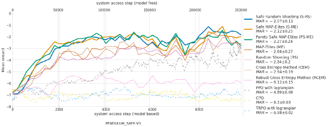
(a)

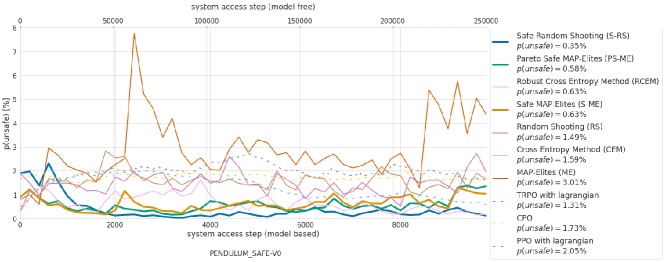
(b)

Figure 4: Mean reward and probability percentage of unsafe results for Pendulum environment with unsafe region. Dashed line indicate Model-free baselines and plain one Model-based approaches. Thicker line represent the proposed algorithms.

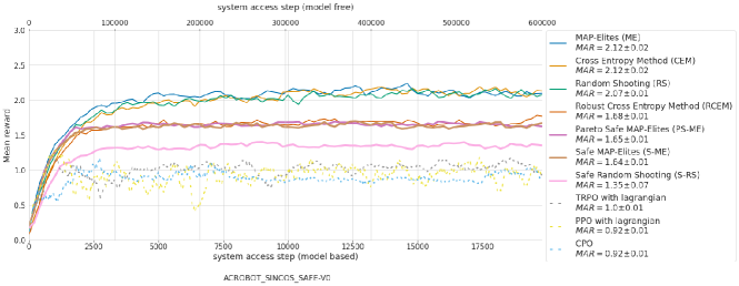
(a)

(b)

Figure 5: Mean reward and probability percentage of unsafe results for Acrobot environment with unsafe region. Dashed line indicate Model-free baselines and plain one Model-based approaches. Thicker line represent the proposed algorithms.

The algorithms are compared according to four metrics: Mean Asymptotic Reward (MAR), Mean Reward Convergence Pace (MRCP), Probability percentage of unsafe (p(unsafe)[%]) and transient probability percentage of unsafe (p(unsafe)[%]_trans).

Table 1: Summary of the different methods on the two different environments Pendulum and Acrobot. MAR is the mean asymptotic reward, MRCP($r_{thr}$) is the number of system access steps needed to achieve $r_{thr}$ of the optimum reward, $p(\text{unsafe})[\%]$ and $p(\text{unsafe})[\%]_{trans}$ are the probability percentage of being unsafe during epochs. All the metrics are average over all epochs and seeds and $\downarrow$ and $\uparrow$ mean lower and higher the better, respectively. The best safe methods with respect to each metric are highlighted in bold. All $\pm$ values are 90% Gaussian confidence interval.

Method	MAR $\uparrow$		MRCP$\times 10^{3}\downarrow$		$p(\text{unsafe})[\%]\downarrow$		$p(\text{unsafe})_{trans}[\%]\downarrow$
	Pendulum $r_{thr}=-2.5$
GuSS (S-RS)	-2.09 $\hskip 2.84544pt\pm\hskip 2.84544pt$	0.09	2.12 $\hskip 2.84544pt\pm\hskip 2.84544pt$	1.45	0.35 $\hskip 2.84544pt\pm\hskip 2.84544pt$	0.63	1.23 $\hskip 1.42271pt\pm\hskip 2.84544pt$	1.28
GuSS (S-ME)	-2.2 $\hskip 2.84544pt\pm\hskip 2.84544pt$	0.16	2.0 $\hskip 2.84544pt\pm\hskip 2.84544pt$	0.9	0.63 $\hskip 2.84544pt\pm\hskip 2.84544pt$	0.57	0.54 $\hskip 1.42271pt\pm\hskip 2.84544pt$	0.57
GuSS (PS-ME)	-2.27 $\hskip 2.84544pt\pm\hskip 2.84544pt$	0.17	2.10 $\hskip 2.84544pt\pm\hskip 2.84544pt$	1	0.58 $\hskip 2.84544pt\pm\hskip 2.84544pt$	0.52	0.6 $\hskip 1.42271pt\pm\hskip 2.84544pt$	0.56
RCEM	-6.12 $\hskip 2.84544pt\pm\hskip 2.84544pt$	0.15	6.7 $\hskip 2.84544pt\pm\hskip 2.84544pt$	0.81	0.63 $\hskip 2.84544pt\pm\hskip 2.84544pt$	0.64	0.84 $\hskip 1.42271pt\pm\hskip 2.84544pt$	0.7
RS	-2.7 $\hskip 2.84544pt\pm\hskip 2.84544pt$	0.14	2.60 $\hskip 2.84544pt\pm\hskip 2.84544pt$	1.2	1.49 $\hskip 2.84544pt\pm\hskip 2.84544pt$	1.0	1.36 $\hskip 1.42271pt\pm\hskip 2.84544pt$	0.61
ME	-2.53 $\hskip 2.84544pt\pm\hskip 2.84544pt$	0.19	1.90 $\hskip 2.84544pt\pm\hskip 2.84544pt$	0.7	3.01 $\hskip 2.84544pt\pm\hskip 2.84544pt$	2.78	2.01 $\hskip 1.42271pt\pm\hskip 2.84544pt$	1.95
CEM	-2.99 $\hskip 2.84544pt\pm\hskip 2.84544pt$	0.15	1.64 $\hskip 2.84544pt\pm\hskip 2.84544pt$	0.41	1.59 $\hskip 2.84544pt\pm\hskip 2.84544pt$	0.89	1.43 $\hskip 1.42271pt\pm\hskip 2.84544pt$	0.85
CPO	-6.06 $\hskip 2.84544pt\pm\hskip 2.84544pt$	0.04	22 $\hskip 2.84544pt\pm\hskip 2.84544pt$	0.0	1.73 $\hskip 2.84544pt\pm\hskip 2.84544pt$	0.92	1.59 $\hskip 1.42271pt\pm\hskip 2.84544pt$	0.78
PPO lag	-4.1 $\hskip 2.84544pt\pm\hskip 2.84544pt$	0.12	138 $\hskip 2.84544pt\pm\hskip 2.84544pt$	65	2.05 $\hskip 2.84544pt\pm\hskip 2.84544pt$	1.75	2.15 $\hskip 1.42271pt\pm\hskip 2.84544pt$	1.48
TRPO lag	-7.02 $\hskip 2.84544pt\pm\hskip 2.84544pt$	0.03	161 $\hskip 2.84544pt\pm\hskip 2.84544pt$	55	1.31 $\hskip 2.84544pt\pm\hskip 2.84544pt$	0.91	2.07 $\hskip 1.42271pt\pm\hskip 2.84544pt$	0.89
	Acrobot $r_{thr}=1.6$
GuSS (S-RS)	1.35 $\hskip 2.84544pt\pm\hskip 2.84544pt$	0.07	1.6 $\hskip 2.84544pt\pm\hskip 2.84544pt$	0.26	1.1 $\hskip 2.84544pt\pm\hskip 2.84544pt$	1.05	1.85 $\hskip 1.42271pt\pm\hskip 2.84544pt$	1.56
GuSS (S-ME)	1.64 $\hskip 2.84544pt\pm\hskip 2.84544pt$	0.01	1.36 $\hskip 2.84544pt\pm\hskip 2.84544pt$	0.25	1.1 $\hskip 2.84544pt\pm\hskip 2.84544pt$	1.22	2.45 $\hskip 1.42271pt\pm\hskip 2.84544pt$	1.92
GuSS (PS-ME)	1.65 $\hskip 2.84544pt\pm\hskip 2.84544pt$	0.01	1.56 $\hskip 2.84544pt\pm\hskip 2.84544pt$	0.11	1.42 $\hskip 2.84544pt\pm\hskip 2.84544pt$	1.62	3.75 $\hskip 1.42271pt\pm\hskip 2.84544pt$	2.77
RCEM	1.68 $\hskip 2.84544pt\pm\hskip 2.84544pt$	0.01	1.60 $\hskip 2.84544pt\pm\hskip 2.84544pt$	0.37	2.01 $\hskip 2.84544pt\pm\hskip 2.84544pt$	1.4	2.85 $\hskip 1.42271pt\pm\hskip 2.84544pt$	1.84
RS	2.07 $\hskip 2.84544pt\pm\hskip 2.84544pt$	0.01	1.28 $\hskip 2.84544pt\pm\hskip 2.84544pt$	0.29	24.8 $\hskip 2.84544pt\pm\hskip 2.84544pt$	8.3	10.85 $\hskip 1.42271pt\pm\hskip 2.84544pt$	7.36
ME	2.12 $\hskip 2.84544pt\pm\hskip 2.84544pt$	0.02	1.12 $\hskip 2.84544pt\pm\hskip 2.84544pt$	0.24	25.6 $\hskip 2.84544pt\pm\hskip 2.84544pt$	7.91	12.18 $\hskip 1.42271pt\pm\hskip 2.84544pt$	7.95
CEM	2.12 $\hskip 2.84544pt\pm\hskip 2.84544pt$	0.02	1.40 $\hskip 2.84544pt\pm\hskip 2.84544pt$	0.43	24.9 $\hskip 2.84544pt\pm\hskip 2.84544pt$	8.91	9.14 $\hskip 1.42271pt\pm\hskip 2.84544pt$	7.17
CPO	0.94 $\hskip 2.84544pt\pm\hskip 2.84544pt$	0.01	87 $\hskip 2.84544pt\pm\hskip 2.84544pt$	59	5.43 $\hskip 2.84544pt\pm\hskip 2.84544pt$	1.74	4.35 $\hskip 1.42271pt\pm\hskip 2.84544pt$	2.49
PPO lag	0.94 $\hskip 2.84544pt\pm\hskip 2.84544pt$	0.01	24 $\hskip 2.84544pt\pm\hskip 2.84544pt$	3	3.7 $\hskip 2.84544pt\pm\hskip 2.84544pt$	1.94	4.02 $\hskip 1.42271pt\pm\hskip 2.84544pt$	2.46
TRPO lag	1.02 $\hskip 2.84544pt\pm\hskip 2.84544pt$	0.01	37 $\hskip 2.84544pt\pm\hskip 2.84544pt$	22	4.2 $\hskip 2.84544pt\pm\hskip 2.84544pt$	2.0	4.31 $\hskip 1.42271pt\pm\hskip 2.84544pt$	2.53

Mean Asymptotic Reward (MAR). Given a trace $\mathcal{T}r$ and a reward $r_{t}=r(s_{t},a_{t})$ obtained at each step $t$, we define the mean reward as $R(\mathcal{T}r)=\frac{1}{T}\sum_{t=1}^{T}r_{t}$. The mean reward in iteration $\tau$ is then $MR(\tau)=R(\mathcal{T}r^{(\tau)}_{t})$. The measure of asymptotic performance (MAR), is the mean reward in the second half of the epochs (we set $N$ so that the algorithms converge after less than $N/2$ epochs) $MAR=\frac{2}{N}\sum_{\tau=N/2}^{N}MR(\tau)$.

Mean Reward Convergence Pace (MRCP). To assess the speed of convergence, we define the MRCP as the number of steps needed to achieve an environment-specific reward threshold $r_{thr}$. The unit of MRCP($r_{thr}$) is real-system access steps, to make it invariant to epoch length, and because it better translates the sample efficiency of the different methods.

Probability percentage of unsafe ($p(\text{unsafe})[\%]$). To compare the safety cost of the different algorithms, we compute the probability percentage of being unsafe during each episode as $p(\text{unsafe})=100*\frac{1}{T}\sum_{k=0}^{T}\mathcal{C}_{k}$ where $T$ is the number of steps per episode. We also compute the transient probability percentage $p(\text{unsafe})_{trans}[\%]$ as a measure to evaluate safety at the beginning of the training phase, usually the riskiest part of the training process. It is computed by taking the mean of $p(\text{unsafe})$ on the first 15% training epochs.

The results are shown in Table 1. The MAR scores and the $p(\text{unsafe})[\%]$ for the pendulum system are shown in Fig. 4, while the ones for the acrobot system are in Fig. 5. Fig. 6 shows the visited states distributions for the Safe Pendulum environment. Additional plots are presented in Appendices D and E.

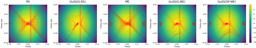
Figure 6: Explored states for Safe Pendulum (first row).For Safe Pendulum a state $s$ corresponds to the angular position and velocity of the pendulum $(\theta,\dot{\theta})$. The states are color coded according to the corresponding reward. The red-shaded area corresponds to the unsafe area. Each point represent an explored state. Red points are safe states while blue points are unsafe ones. The size of the point is proportional to the number of times that state has been visited.

7 Discussion

The results presented in Sec. 6 show how GuSS can reach high performances on both test environments while keeping safety cost low. As expected, on Acrobot, safe methods reach lower MAR scores compared to unsafe ones due to these last ones ignoring the safety constraints. At the same time, this leads to much higher $p(\text{unsafe})$ for unsafe approaches. Interestingly, this is not the case on Pendulum where unsafe approaches tend to have lower MAR scores compared to safe methods even while not respecting safety criteria. The best unsafe method, ME, has in fact a MAR of $-2.53\pm 0.19$ while the worst MBRL safe method, PS-ME, has a MAR of $-2.27\pm 0.17$ $(\text{p}<1e-08)$. This is likely due to the unsafe region effectively halving the search space. The left hand side in fact provides lower "safe rewards" compared to the right hand side, pushing the safe algorithms to focus more on swinging the arm towards the right than the left. This is particularly visible in Fig. 6 between the safe and unsafe methods where the unsafe area cleanly cuts the distribution of visited states. Moreover, while the safe methods, and in particular ME cover a larger part of the state space, the safe ones tend to focus much more on the high rewarding state.

When comparing the performances of the different safe planners for GuSS, it is possible to notice how the simpler S-RS planner outperforms the more complex S-ME and PS-ME on Pendulum with respect to both MAR $(\text{p}<0.02)$ and $p(\text{unsafe})$ $(\text{p}<0.05)$. This is not the case on the more complex Acrobot, where the improved search strategies performed by S-ME and PS-ME reach higher MAR scores compared to S-RS $(\text{p}<0.02)$, while being comparable with respect to the safety cost. This hints at the fact that while a simple strategy like S-RS is very efficient in simple set-ups, more advanced planning techniques are needed in more complex settings. RCEM the closest method to GuSS, failed on Pendulum but reached higher MAR on Acrobot, however with twice the safety cost.

The results also show how model-free approaches require at least one order of magnitude more interactions with the real-system than MBRL methods while still having worse MAR scores and higher safety costs.

8 Conclusion and Future work

In this study, we proposed GuSS, a model based planning method for safe reinforcement learning. We tested the method on two constrained environments and the results show that, while being simple, GuSS provides good results in terms of safety and reward trade-off with minimal computational complexity. Moreover, we observed that in some settings, like Safe Pendulum, the introduction of safety constraints can lead to a better completion of the task. Further experiments are needed to confirm this effect, but if this holds, it could be possible to take advantage of it in a curriculum learning fashion: starting from strict safety constraints and incrementally relaxing them to get to the final task and safety requirement. This could help even more in the application of RL methods to real engineering systems, allowing the engineers handling the system to be more confident in the performances of the methods.

Notwithstanding the great results obtained by our proposed approach, the performances of GuSS are still tied to the accuracy of the model. If the model is wrong, it could easily lead the agent to unsafe states. A possible solution to this is to have uncertainty aware models that can predict their own uncertainty on the sampled trajectories. At the same time, the ME-based safe planners we proposed also suffer from the limitation of many QD approaches, namely the need to hand-design the behavior space. While some works have been proposed to address this issue [10, 27], these add another layer of complexity to the system, possibly reducing performance with respect to the safety constraints.

Appendix A MAP-Elites Pseudocode

Algorithm 2 shows the pseudocode of the MAP-Elites (ME) method.

1 INPUT: real system $p_{\text{real}}$, initial state $s_{0}$, evaluation budget $N$, parameter space $\Phi$, discretized behavior space $\mathcal{B}$, variation function $\mathbb{V}(\cdot)$, number of initial policies $M$, episode length $H$;

2 RESULT: collection of policies $\mathcal{A}_{\text{ME}}$;

3 $\mathcal{A}_{\text{ME}}=\emptyset$ $\triangleright$ Initialize empty collection

4

5$\Gamma\leftarrow\text{SAMPLE}(\Phi,M)$ $\triangleright$ Sample initial $M$ policies

6

7$R,C,\mathcal{T}_{real}=\text{ROLLOUT}(p_{\text{real}},s_{0},\phi_{i},H),~{}~{}\forall\phi_{i}\in\Gamma$ $\triangleright$ Evaluate policies in the real system

8

9$b_{i}=f(\phi_{i},\mathcal{T}^{i}_{real}),\quad\forall\phi_{i}\in\Gamma~{}\text{and}~{}\forall\mathcal{T}^{i}_{real}\in\mathcal{T}_{real}$ $\triangleright$ Calculate policies behavior descriptors

10

11$\mathcal{A}_{\text{ME}}\leftarrow\phi_{i},~{}~{}\forall\phi_{i}\in\Gamma$ $\triangleright$ Store policies in collection

12

13while $N$ not depleted do

14       $\Gamma\leftlsquigarrow\text{SELECT}(\mathcal{A}_{\text{ME}},K,\Phi)$ $\triangleright$ Select $K$ policies from collection

15      

16      $\tilde{\Gamma}\leftlsquigarrow\mathbb{V}(\Gamma)$ $\triangleright$ Generate new policies

17      

18      $R,C,\mathcal{T}_{real}=\text{ROLLOUT}(p_{\text{real}},s_{0},\tilde{\phi}_{i},H),~{}~{}\forall\tilde{\phi}_{i}\in\tilde{\Gamma}$ $\triangleright$ Evaluate new policies in the real system

19      

20      $b_{i}=f(\tilde{\phi}_{i},\mathcal{T}^{i}_{real}),\quad\forall\tilde{\phi}_{i}\in\tilde{\Gamma}~{}\text{and}~{}\forall\mathcal{T}^{i}_{real}\in\mathcal{T}_{real}$ $\triangleright$ Calculate behavior descriptors

21      

22      $\mathcal{A}_{\text{ME}}\leftarrow\tilde{\phi}_{i},~{}~{}\forall\tilde{\phi}_{i}\in\tilde{\Gamma}$ $\triangleright$ Store policies in collection

23      

Algorithm 2 MAP-Elites

Appendix B Planners Pseudocode

This appendix contains the pseudo code of the three planners introduced in the paper. Each planner evaluates a policy on the model through a ROLLOUT function detailed in Alg. 3.

1

2INPUT: model $p$, initial state $s_{0}$, policy $\phi$, horizon length $h$;

3 RESULT: collected reward $R$, collected cost $C$, simulated trace $\mathcal{T}_{model}$;

4

5$\mathcal{T}_{model}=\emptyset$ $\triangleright$ Initialize empty trace

6 for j in [0, …, h] do

7       $a_{j}\leftlsquigarrow\phi(s_{j})$ $\triangleright$ Draw action from policy

8       $s_{j+1}\leftlsquigarrow p(s_{j},a_{j})$ $\triangleright$ Draw next predicted state

9       $\mathcal{T}_{model}=\mathcal{T}_{model}\bigcup(s_{j},a_{j})$ $\triangleright$ Update trace

10      

11$R=\sum_{j=0}^{h}\gamma^{j}r(s_{j},a_{j})$ $\triangleright$ Calculate reward of action sequence

12 $C=\sum_{j=0}^{h}\gamma^{j}c(s_{j},a_{j})$ $\triangleright$ Calculate cost of action sequence

Algorithm 3 ROLLOUT

B.1 Safe Random Shooting

Algorithm 4 shows the pseudocode of the Safe Random Shooting (S-RS) planner.

1 INPUT: model $p$, current real-system state $s_{t}$, planning horizon $h$, evaluated action sequences $N$, action space $\mathcal{A}$;

2 RESULT: action to perform $a_{t}$;

3 $\text{AS}=\emptyset$ $\triangleright$ Initialize empty collection of action sequences

4 for i in [0, …, N] do

5       $\phi_{i}=[a_{t},\dots,a_{t+h}]\leftlsquigarrow\text{SAMPLE}(\mathcal{A},h)$ $\triangleright$ Sample action sequence

6       $R_{i}$, $C_{i}$, $\mathcal{T}^{i}_{model}$ = ROLLOUT($p$, $s_{t}$, $\phi_{i}$, $h$) $\triangleright$ Evaluate action sequence

7       $\text{AS}=\text{AS}\bigcup(\phi_{i},R_{i},C_{i})$ $\triangleright$ Store evaluated action sequence

8      

9$\text{AS}_{\text{lc}}\leftlsquigarrow\text{AS}$ $\triangleright$ Get action sequences with lowest cost

10 $\phi_{\text{best}}\leftlsquigarrow\text{AS}_{\text{lc}}$ $\triangleright$ Get action sequence with highest reward

11 $a_{t}\leftlsquigarrow\phi_{\text{best}}(s_{t})$ $\triangleright$ Get next action

Algorithm 4 S-RS

B.2 Safe MAP-Elites

Algorithm 6 shows the pseudocode of the Safe MAP-Elites (S-ME) method. The SELECT function is shown in Alg. 5.

1 INPUT: Collection of policies $\mathcal{A}_{\text{ME}}$, Number of policies to select $K$, Policy parameter space $\Phi$ ;

2 RESULT: set of selected policies $\Gamma$;

3 $\Gamma=\emptyset$ $\triangleright$ Initialize empty set of selected policies

4

5$\Gamma\leftlsquigarrow\mathcal{A}_{\text{ME}}[C=0]$ $\triangleright$ Select policies with $C=0$ from collection 

6if $\text{size}(\Gamma)<K$ then

7       $\Gamma=\Gamma\bigcup\text{SAMPLE}(\Phi)$ $\triangleright$ Sample missing policies from parameter space

8      

Algorithm 5 SELECT function of S-ME planner

1 INPUT: model $p$, current real-system state $s_{t}$, planning horizon $h$, evaluated action sequences $N$, discretized behavior space $\mathcal{B}$, variation function $\mathbb{V}(\cdot)$, number of initial policies $M$, number of policies per iteration $K$, policy parameter space $\Phi$ ;

2 RESULT: action to perform $a_{t}$;

3 $\mathcal{A}_{\text{ME}}=\emptyset$ $\triangleright$ Initialize empty collection of policies

4

5$\Gamma\leftarrow\text{SAMPLE}(\Phi,M)$ $\triangleright$ Sample initial $M$ policies

6

7$R,C,\mathcal{T}_{model}=\text{ROLLOUT}(p,s_{t},\phi_{i},h),\quad\forall\phi_{i}\in\Gamma$ $\triangleright$ Evaluate policies in the model

8

9$b_{i}=f(\phi_{i},\mathcal{T}^{i}_{model}),\quad\forall\phi_{i}\in\Gamma~{}\text{and}~{}\forall\mathcal{T}^{i}_{model}\in\mathcal{T}_{model}$ $\triangleright$ Calculate policies behavior descriptors

10

11$\mathcal{A}_{\text{ME}}\leftarrow\phi_{i},~{}~{}\forall\phi_{i}\in\Gamma$ $\triangleright$ Store policies in collection

12

13while $N$ not depleted do

14       $\Gamma\leftlsquigarrow\text{SELECT}(\mathcal{A}_{\text{ME}},K,\Phi)$ $\triangleright$ Select $K$ policies with $C=0$ from collection

15      

16      $\tilde{\Gamma}\leftlsquigarrow\mathbb{V}(\Gamma)$ $\triangleright$ Generate new policies

17      

18      $R,C,\mathcal{T}_{model}=\text{ROLLOUT}(p,s_{t},\tilde{\phi}_{i},h),\quad\forall\tilde{\phi}_{i}\in\tilde{\Gamma}$ $\triangleright$ Evaluate new policies in the model

19      

20      $b_{i}=f(\tilde{\phi}_{i},\mathcal{T}^{i}_{model}),\quad\forall\tilde{\phi}_{i}\in\tilde{\Gamma}~{}\text{and}~{}\forall\mathcal{T}^{i}_{model}\in\mathcal{T}_{model}$ $\triangleright$ Calculate behavior descriptors

21      

22      $\mathcal{A}_{\text{ME}}\leftarrow\tilde{\phi}_{i},~{}~{}\forall\tilde{\phi}_{i}\in\tilde{\Gamma}$ $\triangleright$ Store policies in collection

23      

24$\Gamma_{\text{lc}}\leftlsquigarrow\text{AS}$ $\triangleright$ Get policies with lowest cost

25

26$\phi_{\text{best}}\leftlsquigarrow\Gamma_{\text{lc}}$ $\triangleright$ Get policy with highest reward

27

28$a_{t}\leftlsquigarrow\phi_{\text{best}}(s_{t})$ $\triangleright$ Get next action

Algorithm 6 S-ME

B.3 Pareto Safe MAP-Elites

The Pareto Safe MAP-Elites (PS-ME) planner works similarly to the S-ME one with the exception of the SELECT function at line 9 of Alg. 6. So for this planner we just report the pseudocode of this function in Alg. 7.

1 INPUT: Collection of policies $\mathcal{A}_{\text{ME}}$, Number of policies to select $K$, Policy parameter space $\Phi$ ;

2 RESULT: set of selected policies $\Gamma$;

3 $\Gamma=\emptyset$ $\triangleright$ Initialize empty set of selected policies

4

5$[\Gamma^{0}_{\text{ND}},\dots,\Gamma^{n}_{\text{ND}}]\leftlsquigarrow$ NON_DOMINATED_SORT($\mathcal{A}_{\text{ME}}$) $\triangleright$ Sort collection into non dominated fronts

6

7$i=0$

8 while size$(\Gamma)<K$ do

9       $\Gamma\leftlsquigarrow\Gamma^{i}_{\text{ND}}$ $\triangleright$ Select policies from best front

10       $i=i+1$

11      

Algorithm 7 SELECT function of PS-ME planner

Appendix C Training and hyper-parameters selection

All the training of model-based and model-free methods have been perform in parallel with 6 CPU servers. Each server had 16 Intel(R) Xeon(R) Gold CPU’s and 32 gigabytes of RAM.

C.1 Model Based method

Table 2: Model and Agent Hyper-parameters

		Safe Pendulum	Safe Acrobot
	Model
	Optimizer	Adam	Adam
	Learning rate	1e-3	1e-3
(DARMDNdet)	Nb layers	2	2
	Neurons per layer	50	50
	Nb epochs	300	300
	Planning Agents
CEM and RCEM	Horizon	10	10
	Nb actions sequence	20	20
	Nb elites	10	10
S-RS and RS	Horizon	10	10
	Nb actions sequence	100	100
ME, S-ME, PS-ME	Horizon	10	10
	Nb policies	100	100
	Nb initial policies	25	25
	Nb policies per iteration	5	5
	Behavior space grid size	50 $\times$ 50	50 $\times$ 50
	Nb policy params.	26	83
	Nb policy hidden layers	1	2
	Nb policy hidden size	5	5
	Policy activation func.	Sigmoid	Sigmoid

C.2 Model Free method

All model free algorithms implementation and hyper-parameters were taken from the https://github.com/openai/safety-starter-agents repository.

Appendix D Optimality

Safe-RL algorithms have to optimize the reward while minimizing the cost. Choosing which algorithm is the best is a multi-objective optimization problem. Fig. 7 shows where each of the methods tested in this paper resides with respect to the MAR score and the p(unsafe). Methods labeled with the same number belong to the same optimality front with respect to the two metrics. A lower label number indicates an higher performance of the method.

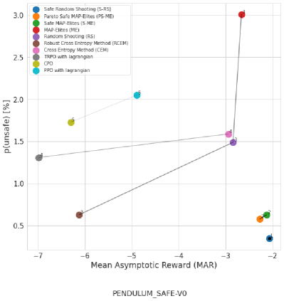
(a)

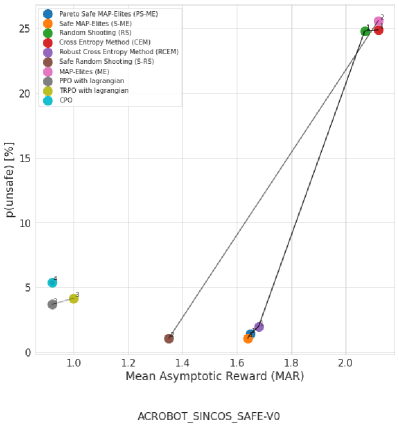
(b)

Figure 7:

Appendix E Exploration plots

In this section we present plots about the explored state distribution for the different algorithms on the two environments.

The State Coverage plots, leftmost one in the figures, represents the density of times a state has been explored. The unsafe area is highlighted in red.

The Reward Heatmap plots, center ones, show the distribution of the visited states overimposed to the reward landscape. The unsafe area is highlighted in red.

The Reward bins plots, rightmost ones, show the histogram of visited stated with respect to the reward of that state. The histograms are generated by dividing the interval between the minimum and maximum reward possible in the environment into 10 buckets and counting how many visited states obtain that reward.

It is possible to see on the reward plots for the Safe Acrobot environment in Appendix E.2 how the safety constraint limits the number of times the states with $r>3$ are visited by safe methods compared to unsafe ones.

E.1 Safe Pendulum

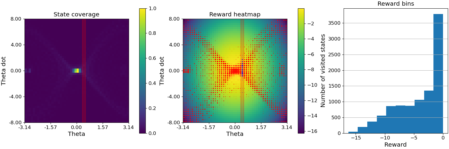
Figure 8: Exploration plot for RS on Safe Pendulum.

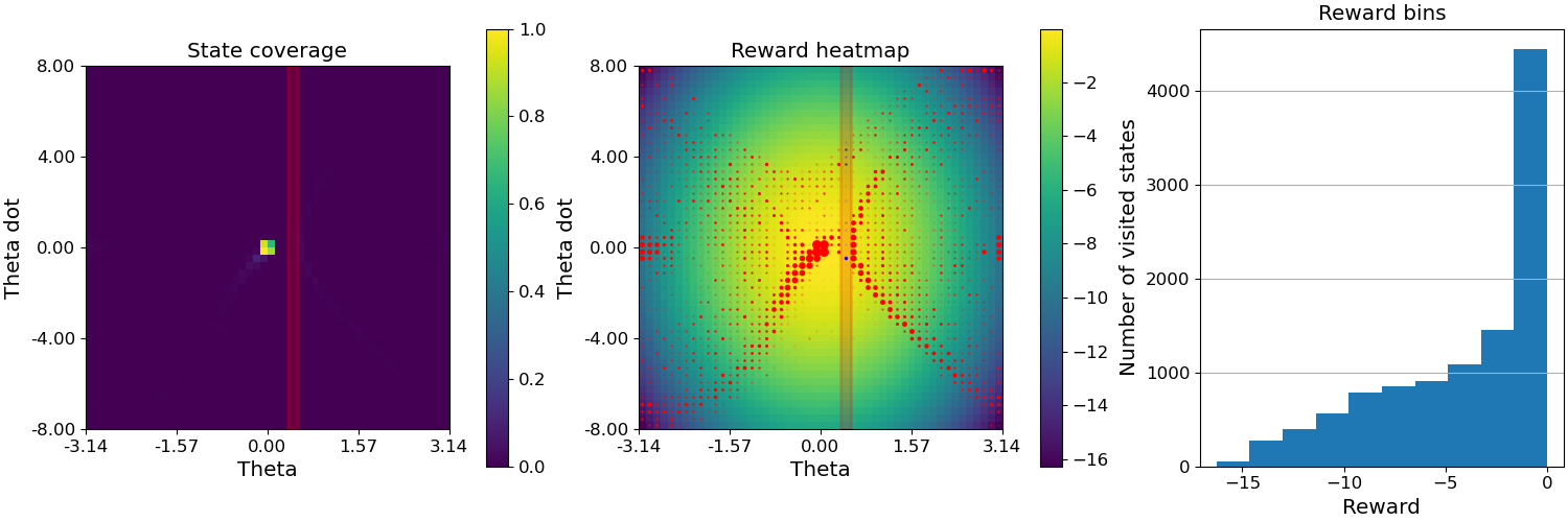
Figure 9: Exploration plot for GuSS (S-RS) on Safe Pendulum.

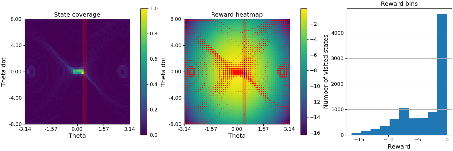
Figure 10: Exploration plot for ME on Safe Pendulum.

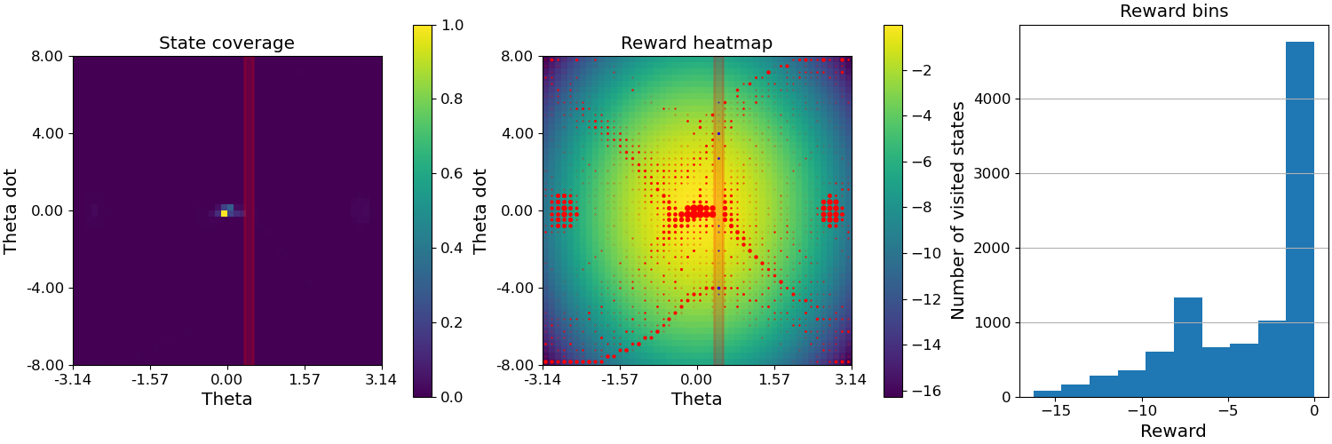
Figure 11: Exploration plot for GuSS (S-ME) on Safe Pendulum.

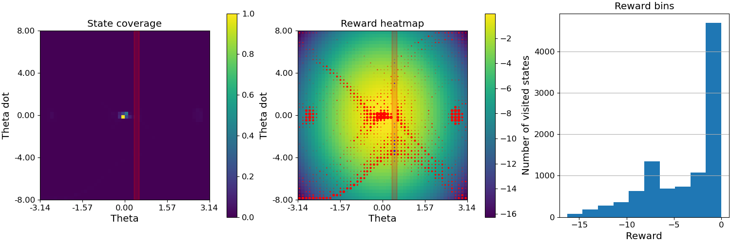
Figure 12: Exploration plot for GuSS (PS-ME) on Safe Pendulum.

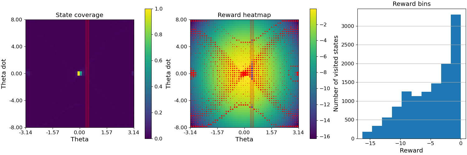
Figure 13: Exploration plot for CEM on Safe Pendulum.

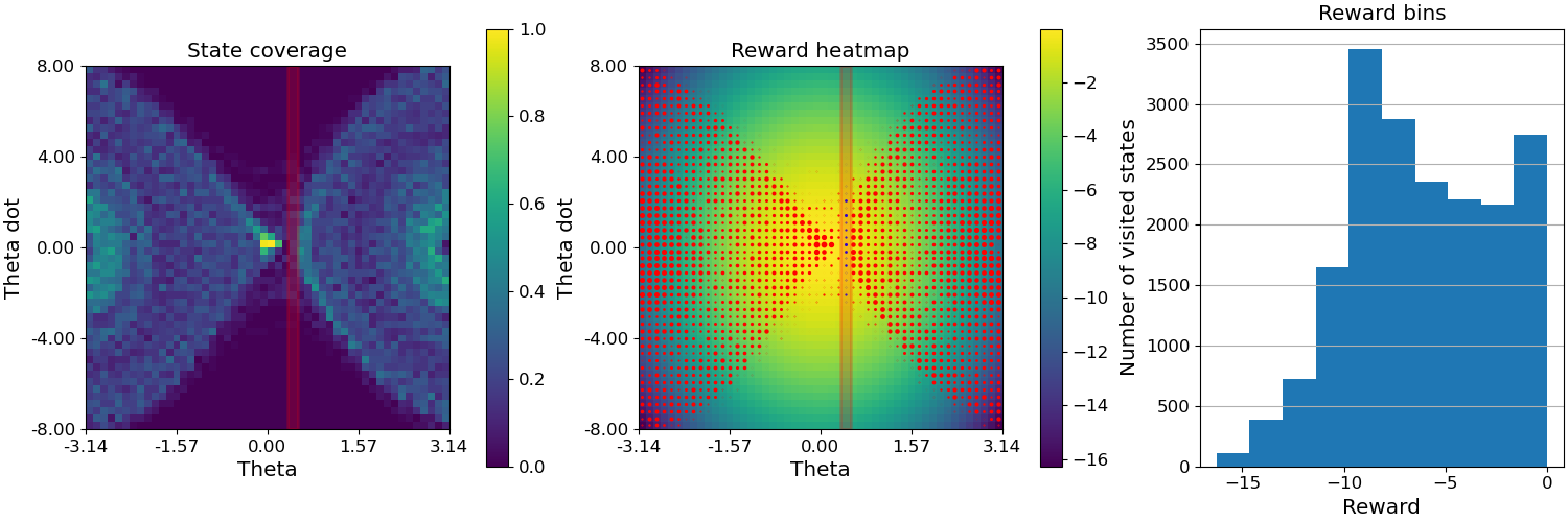
Figure 14: Exploration plot for RCEM on Safe Pendulum.

E.2 Safe Acrobot

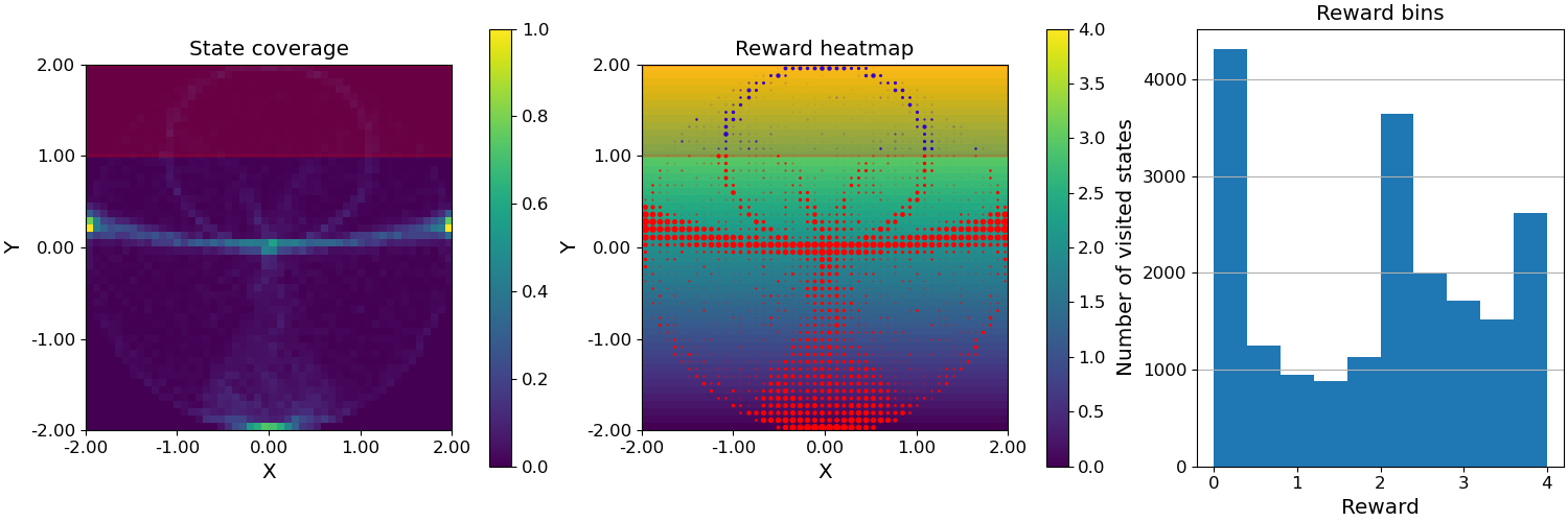
Figure 15: Exploration plot for RS on Safe Acrobot.

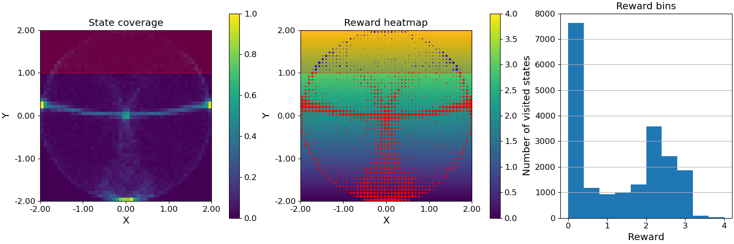
Figure 16: Exploration plot for GuSS (S-RS) on Safe Acrobot.

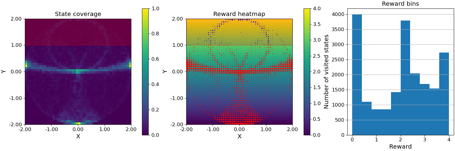
Figure 17: Exploration plot for ME on Safe Acrobot.

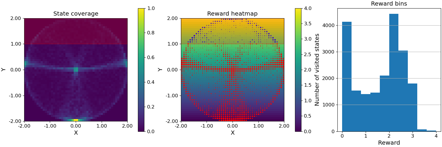
Figure 18: Exploration plot for GuSS (S-ME) on Safe Acrobot.

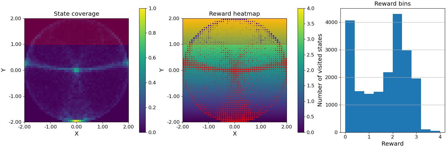
Figure 19: Exploration plot for GuSS (PS-ME) on Safe Acrobot.

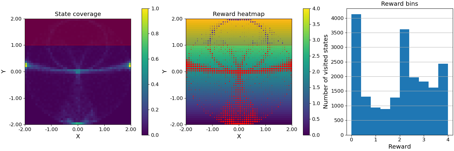
Figure 20: Exploration plot for CEM on Safe Acrobot.

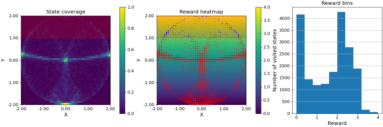
Figure 21: Exploration plot for RCEM on Safe Acrobot.

References

- [1] Joshua Achiam, David Held, Aviv Tamar and Pieter Abbeel “Constrained policy optimization” In International conference on machine learning, 2017, pp. 22–31 PMLR
- [2] Eitan Altman “Constrained Markov decision processes: stochastic modeling” Routledge, 1999
- [3] Dario Amodei et al. “Concrete problems in AI safety” In arXiv preprint arXiv:1606.06565, 2016
- [4] OpenAI: Marcin Andrychowicz et al. “Learning dexterous in-hand manipulation” In The International Journal of Robotics Research 39.1 SAGE Publications Sage UK: London, England, 2020, pp. 3–20
- [5] Christopher M Bishop “Mixture density networks” Aston University, 1994
- [6] Greg Brockman et al. “Openai gym” In arXiv preprint arXiv:1606.01540, 2016
- [7] Yinlam Chow, Mohammad Ghavamzadeh, Lucas Janson and Marco Pavone “Risk-constrained reinforcement learning with percentile risk criteria” In The Journal of Machine Learning Research 18.1 JMLR. org, 2017, pp. 6070–6120
- [8] Kurtland Chua, Roberto Calandra, Rowan McAllister and Sergey Levine “Deep reinforcement learning in a handful of trials using probabilistic dynamics models” In Advances in neural information processing systems 31, 2018
- [9] Alexander I Cowen-Rivers et al. “Samba: Safe model-based & active reinforcement learning” In Machine Learning Springer, 2022, pp. 1–31
- [10] Antoine Cully “Autonomous skill discovery with quality-diversity and unsupervised descriptors” In Proceedings of the Genetic and Evolutionary Computation Conference, 2019, pp. 81–89
- [11] Antoine Cully and Yiannis Demiris “Quality and diversity optimization: A unifying modular framework” In IEEE Transactions on Evolutionary Computation 22.2 IEEE, 2017, pp. 245–259
- [12] Carlos E Garcia, David M Prett and Manfred Morari “Model predictive control: Theory and practice—A survey” In Automatica 25.3 Elsevier, 1989, pp. 335–348
- [13] Hao-Lun Hsu, Qiuhua Huang and Sehoon Ha “Improving Safety in Deep Reinforcement Learning using Unsupervised Action Planning” In arXiv preprint arXiv:2109.14325, 2021
- [14] Balázs Kégl, Gabriel Hurtado and Albert Thomas “Model-based micro-data reinforcement learning: what are the crucial model properties and which model to choose?” In arXiv preprint arXiv:2107.11587, 2021
- [15] Prashanth La and Mohammad Ghavamzadeh “Actor-critic algorithms for risk-sensitive MDPs” In Advances in neural information processing systems 26, 2013
- [16] Sascha Lange, Thomas Gabel and Martin Riedmiller “Batch reinforcement learning” In Reinforcement learning Springer, 2012, pp. 45–73
- [17] Nevena Lazic et al. “Data center cooling using model-predictive control” In Advances in Neural Information Processing Systems 31 Curran Associates, Inc., 2018, pp. 3814–3823
- [18] Joel Lehman and Kenneth O Stanley “Evolving a diversity of virtual creatures through novelty search and local competition” In Proceedings of the 13th annual conference on Genetic and evolutionary computation, 2011, pp. 211–218
- [19] Zuxin Liu et al. “Constrained Model-based Reinforcement Learning with Robust Cross-Entropy Method” In arXiv preprint arXiv:2010.07968, 2020
- [20] Carlos Luis “SwingUp Pendulum”, https://gym.openai.com/envs/Pendulum-v0/
- [21] Yecheng Jason Ma, Andrew Shen, Osbert Bastani and Dinesh Jayaraman “Conservative and Adaptive Penalty for Model-Based Safe Reinforcement Learning” In arXiv preprint arXiv:2112.07701, 2021
- [22] Tatsuya Matsushima et al. “Deployment-Efficient Reinforcement Learning via Model-Based Offline Optimization” In International Conference on Learning Representations, 2021
- [23] Volodymyr Mnih et al. “Human-level control through deep reinforcement learning” In nature 518.7540 Nature Publishing Group, 2015, pp. 529–533
- [24] Thomas M. Moerland, Joost Broekens and Catholijn M. Jonker “Model-based Reinforcement Learning: A Survey” In arXiv preprint arXiv:2006.16712, 2021 arXiv:2006.16712 [cs.LG]
- [25] Jean-Baptiste Mouret and Jeff Clune “Illuminating search spaces by mapping elites” In arXiv preprint arXiv:1504.04909, 2015
- [26] Giuseppe Paolo, Alexandre Coninx, Stéphane Doncieux and Alban Laflaquière “Sparse reward exploration via novelty search and emitters” In Proceedings of the Genetic and Evolutionary Computation Conference, 2021, pp. 154–162
- [27] Giuseppe Paolo, Alban Laflaquiere, Alexandre Coninx and Stephane Doncieux “Unsupervised learning and exploration of reachable outcome space” In 2020 IEEE International Conference on Robotics and Automation (ICRA), 2020, pp. 2379–2385 IEEE
- [28] Justin K Pugh, Lisa B Soros and Kenneth O Stanley “Quality diversity: A new frontier for evolutionary computation” In Frontiers in Robotics and AI 3 Frontiers, 2016, pp. 40
- [29] Alex Ray, Joshua Achiam and Dario Amodei “Benchmarking safe exploration in deep reinforcement learning” In arXiv preprint arXiv:1910.01708 7, 2019, pp. 1
- [30] Erica Salvato, Gianfranco Fenu, Eric Medvet and Felice Andrea Pellegrino “Crossing the Reality Gap: a Survey on Sim-to-Real Transferability of Robot Controllers in Reinforcement Learning” In IEEE Access IEEE, 2021
- [31] John Schulman et al. “Trust region policy optimization” In International conference on machine learning, 2015, pp. 1889–1897 PMLR
- [32] David Silver et al. “Mastering the game of Go with deep neural networks and tree search” In nature 529.7587 Nature Publishing Group, 2016, pp. 484–489
- [33] Satinder Singh, Tommi Jaakkola and Michael Jordan “Reinforcement learning with soft state aggregation” In Advances in neural information processing systems 7, 1994
- [34] Richard S Sutton and Andrew G Barto “Reinforcement learning: An introduction” MIT press, 2018
- [35] Chen Tessler, Daniel J Mankowitz and Shie Mannor “Reward constrained policy optimization” In arXiv preprint arXiv:1805.11074, 2018
- [36] Stefan Radic Webster and Peter Flach “Risk Sensitive Model-Based Reinforcement Learning using Uncertainty Guided Planning” In arXiv preprint arXiv:2111.04972, 2021
- [37] Min Wen and Ufuk Topcu “Constrained cross-entropy method for safe reinforcement learning” In Advances in Neural Information Processing Systems 31, 2018
- [38] Tsung-Yen Yang, Justinian Rosca, Karthik Narasimhan and Peter J Ramadge “Accelerating safe reinforcement learning with constraint-mismatched policies” In arXiv preprint arXiv:2006.11645, 2020
- [39] Tsung-Yen Yang, Justinian Rosca, Karthik Narasimhan and Peter J Ramadge “Projection-based constrained policy optimization” In arXiv preprint arXiv:2010.03152, 2020
- [40] Denis Yarats et al. “Don’t Change the Algorithm, Change the Data: Exploratory Data for Offline Reinforcement Learning” In arXiv preprint arXiv:2201.13425, 2022
- [41] Yiming Zhang, Quan Vuong and Keith Ross “First order constrained optimization in policy space” In Advances in Neural Information Processing Systems 33, 2020, pp. 15338–15349