Geo-NI: Geometry-aware Neural Interpolation for Light Field Rendering

Abstract

In this paper, we present a Geometry-aware Neural Interpolation (Geo-NI) framework for light field rendering. Previous learning-based approaches either rely on the capability of neural networks to perform direct interpolation, which we dubbed Neural Interpolation (NI), or explore scene geometry for novel view synthesis, also known as Depth Image-Based Rendering (DIBR). Instead, we incorporate the ideas behind these two kinds of approaches by launching the NI with a novel DIBR pipeline. Specifically, the proposed Geo-NI first performs NI using input light field sheared by a set of depth hypotheses. Then the DIBR is implemented by assigning the sheared light fields with a novel reconstruction cost volume according to the reconstruction quality under different depth hypotheses. The reconstruction cost is interpreted as a blending weight to render the final output light field by blending the reconstructed light fields along the dimension of depth hypothesis. By combining the superiorities of NI and DIBR, the proposed Geo-NI is able to render views with large disparity with the help of scene geometry while also reconstruct non-Lambertian effect when depth is prone to be ambiguous. Extensive experiments on various datasets demonstrate the superior performance of the proposed geometry-aware light field rendering framework.

I Introduction

Light field (LF) describes rays travelling from all directions in a free space [1], demultiplexing the angular information lost in conventional 2D imaging. Benefits from the LF rendering technologies [1, 2], LF enables to reproduce photorealistic views in real-time, enabling travelling freely in metaverse. Standard LF rendering technologies require a Nyquist rate view sampling, i.e., densely-sampled LF with disparities between adjacent views to be less than one pixel [3]. However, existing densely-sampled LF devices or systems [4] either suffers from a long period of acquisition time or falls into the well-known resolution trade-off problem, i.e., sacrificing the spatial resolution for a dense sampling in the angular domain.

With the success of deep learning in artificial intelligence [5], recent researches [6, 7, 8, 9] are stepping towards deep learning-based interpolation, which we refer to as Neural Interpolation (NI), or Depth Image-Based Rendering (DIBR) using a sparsely-sampled LF in the angular domain. On the one hand, typical learning-based NI methods [10, 7, 11] directly map the low angular resolution LF to densely-sampled LF through diverse network architectures. These methods are highly effective in modelling non-Lambertian effects. Nevertheless, the perception range (receptive filed) of the network [12, 13] limits the performance on LF with large disparities, leading to aliasing effects in the reconstructed LF. On the other hand, state-of-the-art learning-based DIBR methods [6, 9, 14] resort to depth estimation followed by view synthesis, which is considered to be a more efficient way to deal with the large disparity issue than only relying on the receptive filed. But these methods require depth consistency along the angular dimension, and thus, often fail to handle the depth ambiguity caused by the non-Lambertian effect.

In this paper, we propose a learning-based framework for geometry-aware LF rendering to address the non-Lambertian and large disparity issues by launching the NI within a novel DIBR pipeline. We term the framework as Geo-NI, as shown in Fig. 1. Specifically, we bridge the gap between the standard NI and DIBR by shearing the input LF with a set of depth hypotheses. The NI part is achieved via a neural network that directly interpolates the sheared LFs. Then the DIBR part is implemented via another neural network to assess the reconstruction quality of the neural interpolated LFs under the depth hypotheses. The DIBR part constructs a cost volume, where each value in the volume can be interpreted as a weight for blending the final rendered (output) LF, as shown in Fig. 1. We therefore name the volume reconstruction cost volume. By incorporating the two parts, the proposed Geo-NI framework is able to synthesize views with large disparity while also reconstruct non-Lambertian effect when depth is prone to be ambiguous.

To efficiently extract high-level LF feature in the NI and DIBR parts, we propose a hierarchical packing-unpacking structure that is able to encode and decode the LF features. The building block of the packing/unpacking structure is spatial-to-channel/channel-to-spatial pixel shuffling followed by convolutional layers. With the help of the spatial-channel pixel shuffling, the networks in Geo-NI are able to efficiently gain a large perceptive field by intactly compressing the spatial resolution and restore it without losing high frequencies. In summary, we make the following contributions:

• A Geometry-aware Neural Interpolation (Geo-NI) framework that joints neural interpolation and depth-based view synthesis for solving non-Lambertian and large disparity challenges in an end-to-end manner;

• A novel reconstruction cost volume derived from the DIBR pipeline that guides the blending of the LFs sheared by different depth hypotheses as well as the rendering of scene depth, as shown in Fig, 1;

• A hierarchical packing-unpacking structure that efficiently encodes and decodes the LF features via spatial-channel pixel shuffling.

We demonstrate the superiority of the proposed Geo-NI framework by performing extensive evaluations on various LF datasets. The proposed network presents high-quality DSLF on challenging cases with both non-Lambertian effects and large disparities.

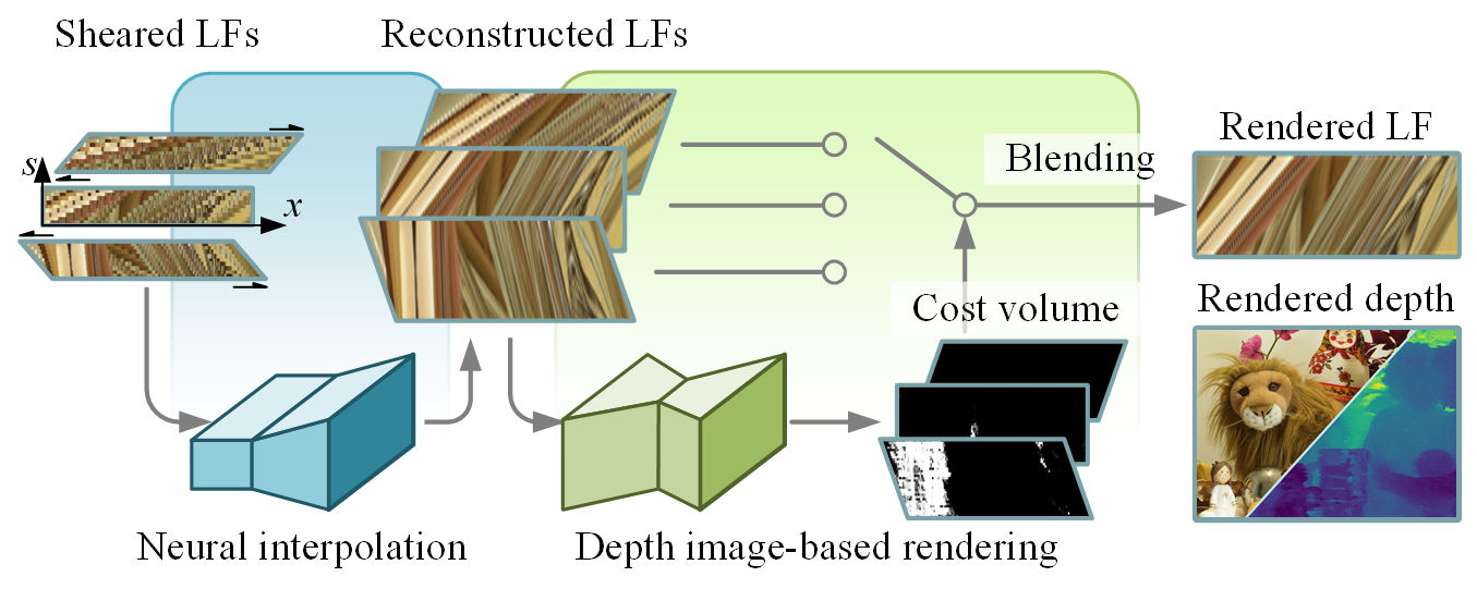
Figure 1: We present Geo-NI framework for geometry-aware light field rendering by launching the Neural Interpolation (NI) within a novel Depth Image-Based Rendering (DIBR) pipeline. The proposed framework is able to render LFs with large disparity while also reconstruct the non-Lambertian effects. LF courtesy of Adhikarla et al. [15].

II Related Work

II-A Plenoptic Sampling and Reconstruction

These approaches treat LF reconstruction as the approximation of plenoptic function using a set of samples. The analysis tools in the Fourier domain show that the sampling produces spectrum replicas along the sample dimensions. Under sparse sampling, the replicas will overlap with its original spectrum, resulting aliasing effects in the LF signals. Classical approaches by Chai et al. [16] and Zhang et al. [17] formulate the reconstruction as filtering of the aliasing high-frequencies while keeping the original spectrum as completely as possible. In [18], Vagharshakyan et al. explored a shearlet transform of composite directions and scales in the Fourier domain to remove the aliasing high-frequencies. To handle the occlusion problem, Zhu et al. [19] proposed an occlusion field theory to quantify the occlusion degree, and designed a reconstruction filter to compensate the missing information caused by the occlusion.

Researchers also focus on training a deep neural network to directly inference the densely-sampled LF from the low angular resolution input [10, 7, 11, 20]. We term this kind of approaches as Neural Interpolation (NI) since they regard the reconstruction as a learning-based interpolation problem of the missing pixels (samples) without exploiting scene geometry. An initial work by Yoon et al. [10] first interpolates the low angular resolution LF with bicubic operation, then employs a convolutional network to refine the reconstructed LF. For explicitly handling the aliasing effects, Wu et al. [7] proposed a “blur-restoration-deblur” framework that first suppresses the high frequency components in the spatial dimension and then restores them via a non-blind deconvolution. Wang et al. [21] applied 3D convolution layers to reconstruct the two angular dimensions of the input LF sequentially. However, the small perception range, i.e., receptive filed [12, 13], impedes the networks to capture long-term correspondences in the input LF, resulting limited performances.

Recent works resort to a deeper network or an efficient architectures to enlarge the receptive field. Yeung et al. [11] directly fed the entire 4D LF into a pseudo 4D convolutional network, and proposed a novel spatial-angular alternating convolution to iteratively refine the angular dimensions of the LF. Jin et al. [14] further extended the spatial-angular alternating convolution to the problem of compressive LF reconstruction. Zhu et al. [20] introduced an U-net architecture to enlarge the receptive field using strided convolutional layers and convLSTM layers [23]. Liu et al. [24], Zhang et al. [25] and Meng et al. [26] applied residual blocks [27] and dense blocks [28] to prevent gradient vanishment when increasing the depth of the networks. Ying et al. [22] proposed a LF disentangling mechanism to disentangle the coupled spatial-angular information by using dilated and strided convolutions directly on the macro-pixel image. However, since the actual size of the receptive field can be smaller than its theoretical size [13], simply pursuing a deeper network without modeling the scene geometry still limits the performance of NI-based approaches.

II-B Depth Image-based Rendering

These approaches first estimate the scene geometry (or depth), then warp the input images to the target viewpoint according to the estimated geometry and blend them. Standard LF depth estimation approaches follow the pipeline of stereo matching [29], which consists of feature description (extraction), cost computation, cost aggregation (or cost volume filtering), depth regression and post refinement. Because the difference of the data attribute, LF provides various depth cues for the feature description and cost computation, e.g., structure tensor-based local direction estimation [30], orthographic Hough transform for curve estimation [31], depth from correspondence [32], depth from defocus [33, 34] and depth from parallelogram cues [35]. Some recent learning-based approaches also explored the cost aggregation and depth regression in the aforementioned pipeline with 2D or 3D convolution networks [36, 37].

For rendering or synthesizing a novel view, typical DIBR approaches first warp the input views to the novel viewpoint with sub-pixel accuracy and then blend them using different strategy, such as total variation optimization [30], soft blending [38] and learning-based synthesis [39, 40, 41]. The most representative DIBR approaches [42, 6] using deep learning techniques employ a sequential network setting, and train the network models by minimizing errors between the synthesized views and the desired outputs (labels). An initial work by Kalantari et al. [6] proposed an end-to-end DIBR framework using two sequential networks to infer depth and color, respectively. Following this setting, Shi et al. [43] proposed to render novel views by blending the warped images in both pixel-level and feature-level. Meng et al. [44] introduced a network for estimating warping confidences that address the errors around occlusion regions. Jin et al. proposed a spatial-angular alternating refinement network for images warped by using a regular sampling pattern (four corner views) [45] and a flexible sampling pattern [46].

Different from the sequential network settings, recent researches [47, 48] focus on decomposing input RGB images into depth-dependent layers, which is dubbed Multi-Plane Image (MPI). For example, Zhou et al. [47] proposed a learning-based framework that infers a single MPI and a background image from two stereo images and synthesizes novel views via alpha blending. Based on this pioneer work, Mildenhall et al. [9] proposed to infer an MPI for each view in the input LF and synthesize novel views by blending the local MPIs.

The aforementioned DIBR approaches directly blending the views warped according to the depth map or depth-related layers, which is highly effective for scenes with large disparity. However, since the depth information is deduced based on the Lambertian assumption, it will appear ambiguity around non-Lambertian regions, resulting in ghosting effects in the synthesized views. In this paper, instead of directly performing pixel or layer-wise warping using depth information, we propose to render the entire high-angular resolution LF by blending the neural interpolated LFs. Due to the NI does not rely on depth information, the proposed Geo-NI framework shows higher reconstruction quality around non-Lambertian regions.

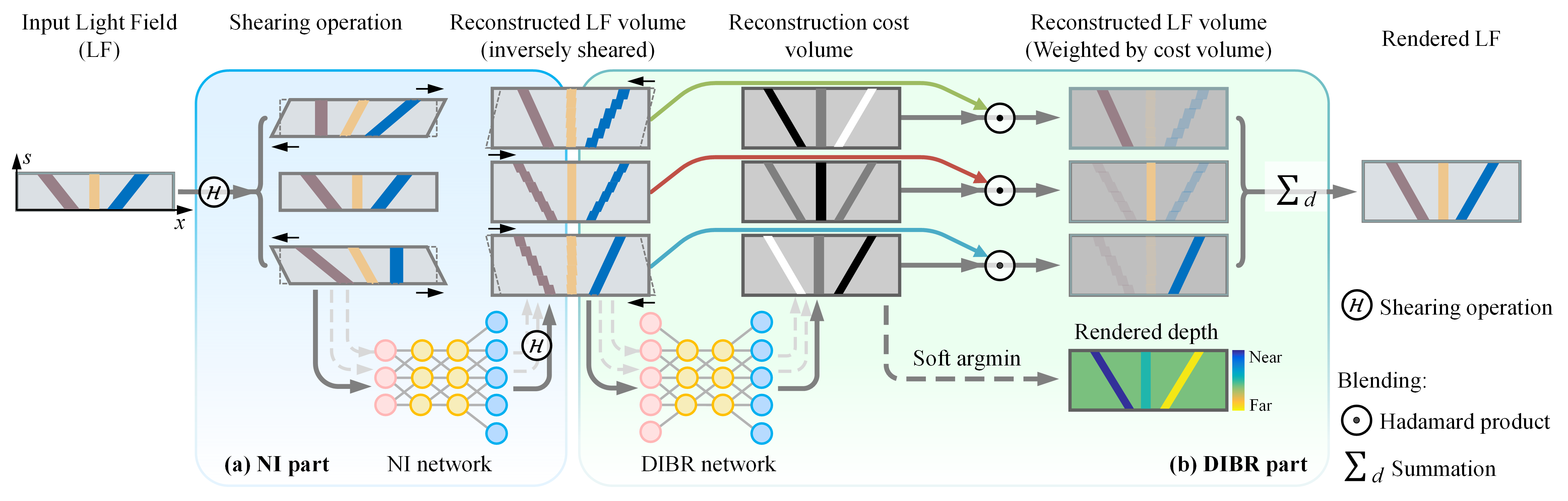
Figure 2: The proposed Geo-NI framework is composed of two parts: (a) a Neural Interpolation (NI) part that directly reconstructs the sheared LF (Sec. III-B); and (b) a Depth Image-Based Rendering (DIBR) part that assigns a reconstruction cost map to each reconstructed LF (Sec. III-B). The DIBR part then blend the reconstructed LFs according to the reconstruction cost. The input is a 3D slice ($L(u,v,s)$ or $L(v,u,t)$) of the LF. We visualize the slices as 2D EPIs for better understanding.

III Methodology

A LF can be parameterized as a 4D function using two-plane representation [1], i.e., $\mathbb{L}(x,y,s,t)\in\mathbb{R}^{W\times H\times A_{s}\times A_{t}}$ with $(x,y)$ denoting the spatial plane and $(s,t)$ the angular plane. A sub-aperture image is obtained by fixing two angular dimensions of the 4D LF $I(x,y)=\mathbb{L}_{s^{*},t^{*}}(x,y)$. An Epipolar Plane Image (EPI) is extracted by fixing one spatial dimension and one angular dimension, $E(x,s)=\mathbb{L}_{y^{*},t^{*}}(x,s)$ or $E(y,t)=\mathbb{L}_{x^{*},s^{*}}(y,t)$. In this paper, we use 3D LF slice with two spatial dimensions and one angular dimension, i.e., $L(x,y,s)=\mathbb{L}_{t^{*}}(x,y,s)$ or $L(y,x,t)=\mathbb{L}_{s^{*}}(x,y,t)$. By splitting LFs into 3D slices, the proposed method can be applied to both 3D LFs from a single-degree-of-freedom gantry system [15, 49] and 4D LFs from plenoptic camera [50] or camera array system. For the reconstruction of a 4D LF $\mathbb{L}(x,y,s,t)$, we employ a hierarchical reconstruction strategy introduced in [7]. In the first step, we first reconstruct 3D LFs using slices $\mathbb{L}_{t^{*}}(x,y,s)$ and $\mathbb{L}_{s^{*}}(x,y,t)$ as input. We then apply the previously reconstructed 3D slices to synthesize the final 4D LF.

In this section, we first introduce the Geometry-aware Neural Interpolation (Geo-NI) framework in Sec. III-A, then discuss the relation between the Geo-NI and standard DIBR pipeline in Sec. V-B, and finally present the proposed hierarchical packing-unpacking structure in details (Sec. III-B).

III-A Geometry-aware Neural Interpolation Framework

In this paper, we hope to design a geometry-aware LF rendering framework that promises to solve the non-Lambertian and large disparity issues in an end-to-end manner. Our proposal is to solve these issues by implanting the characteristic of NI into a DIBR pipeline. The overall framework is depicted in Fig. 2. In the following, we will explain the details of the proposed framework according to the order of the dataflow.

Shearing operation. It is an essential module that bridges the NI part and the DIBR part in the proposed framework. The shearing operation directly alters disparity by shifting all the sub-aperture images synchronously [51, 33]. For an input 3D LF slice $L(x,y,s)$ (or $L(y,x,t)$), we first shear it with a set of depth hypotheses $d\in D$. The shearing operation can be formulate as follows

$$\mathcal{H}_{d}(L(x,y,s))=L(x+(s-\frac{S}{2})\cdot d,y,s),$$ (1)

where $\mathcal{H}_{d}(\cdot)$ denotes the shearing operation with depth hypothesis $d$ and $S$ is the angular resolution of the input LF slice. The vanilla implementation in [51, 33] describes the shearing operation as $L(x+s\cdot d,y,s)$. We add the term $-\frac{S}{2}\cdot d$ to avoid losing too many boundary pixels in the spatial dimension $x$. Besides, in our implementation we use zero padding for the blank regions caused by the shearing operation.

Neural interpolation. The shearing operation generates $D$ sheared LF slices $\mathcal{H}_{d\sim D}(L(x,y,s))$ as indicated in Fig. 2(a). We then feed the slices into a neural network, which we dubbed NI network, to directly reconstruct them into high angular resolution LFs. This step can be denoted as

$$\bar{L}_{d}(x,y,s)=f_{N}(\mathcal{H}_{d}(L(x,y,s));\theta),$$

where $f_{N}(\cdot;\theta)$ is the NI network with trainable parameters $\theta$. Detailed configuration of the NI network will be introduced in Sec. III-B. Note that the reconstructed LFs after this step are still under the deformation effect of the shearing operation. Therefore, we apply another shearing operation to eliminate this effect after the plenoptic reconstruction, which is termed as inverse shearing for short. This step can be denoted as

$$\tilde{L}_{d}(x,y,s)=\mathcal{H}_{-\frac{d}{\alpha}}(\bar{L}_{d}(x,y,s)),$$

where $\alpha$ is the upsampling factor in the angular dimension and $\mathcal{H}$ is the shearing operation described in Eqn. 1. Due to the reconstruction, the shear amount in the inverse shearing operation is $-\frac{d}{\alpha}$ rather than $-d$.

Reconstruction cost volume. In this step, we define the aliasing in reconstructed LF as a kind of cost, which is similar with the matching cost in typical depth estimation or DIBR. We term the cost as reconstruction cost. After the reconstruction and the inverse shearing, we feed the slices $\tilde{L}_{d\sim D}(x,y,s)$ into another neural network, which is termed as DIBR network, as shown in Fig. 2(b). The DIBR network outputs a reconstruction cost volume $\mathcal{C}_{d\sim D}(x,y,s)$ that indicates the aliasing degree of the reconstructed LFs. This step can be described as

$$\mathcal{C}_{d}(x,y,s)=f_{D}(\tilde{L}_{d}(x,y,s);\vartheta),d\in D,$$

where $f_{D}(\cdot;\vartheta)$ denotes the DIBR network with trainable parameters $\vartheta$. Detailed configuration of the DIBR network will be introduced in Sec. III-B. Despite the objective of the proposed Geo-NI is LF reconstruction, we can conveniently render a depth map from the DIBR network. Please refer to Sec. V-A for detail.

Blending. The final rendered high-angular resolution LF $\hat{L}(x,y,s)$ is obtained by blending the reconstructed LFs sheared by all the depth hypotheses $\tilde{L}_{d\sim D}(x,y,s)$. In this perspective, the reconstruction cost volume $\mathcal{C}_{d\sim D}(x,y,s)$ is considered as weight maps. While directly weighting each reconstructed LF $\tilde{L}_{d}$ by reconstruction cost $\mathcal{C}_{d}$ will cause numerical instability. We therefore use normalized cost to formulate the blending

$$\begin{split}\hat{L}(x,y,s)&=\sum_{d}\tilde{L}_{d}(x,y,s)\odot\sigma_{d}(-\mathcal{C}_{d}(x,y,s)),\\ \sigma_{d}(-\mathcal{C}_{d}(x,y,s))&=\frac{\exp(-\mathcal{C}_{d}(x,y,s))}{\sum_{d}\exp(-\mathcal{C}_{d}(x,y,s))},\end{split}$$ (2)

where $\odot$ is the Hadamard product, i.e., element-wise multiplication and $\sigma_{d}$ is the softmax function. It should be noted that a smaller reconstruction cost indicates less degree of aliasing effect in the reconstructed LF, i.e., a higher reconstruction quality. We therefore normalize the reconstruction cost volume $\mathcal{C}_{d\sim D}(x,y,s)$ using softmin nonlinearity in Eqn. 2.

III-B Packing-Unpacking Network

Typical learning-based reconstruction methods [52, 47, 9, 53] pursue a larger size of receptive field through spatial downsampling to achieve a higher reconstruction quality, e.g., strided convolutions, max-pooling and average-pooling. However, recent researches [54, 55, 56] show that the commonly used downsampling methods ignore the sampling theorem, leading to performance degradation for tasks requiring fine-grained details. In comparison, we propose a novel hierarchical packing-unpacking structure that is able to efficiently increasing the receptive field while also preserving high frequency details for LF reconstruction, as shown in Fig. 3(a). In the following, we first introduce the proposed packing-unpacking structure, and then present the NI and DIBR networks constructed based on the structure.

III-B1 Hierarchical packing-unpacking structure

In a packing block, we encode high spatial resolution LF (features) into high-level features by using a Spatial-to-Channel Pixel Shuffling (S2C-PS) [57] followed by a residual module [27] of two convolutional layers, as shown in the left part of Fig. 3(b). Analogously, in an unpacking block we replace the S2C-PS with its reverse operation, Channel-to-Spatial Pixel Shuffling (C2S-PS), to achieve the decode, as shown in the right part of Fig. 3(b). Different with the vanilla version in [57], we only fold one spatial dimension of feature maps into extra feature channels since the depth information is mainly weaved in one spatial dimension on the epipolar plane, as shown in Fig. 3(c). For example, the 5D feature tensor $\phi\in\mathbb{R}^{B\times W\times H\times A\times C}$ is converted to $\phi^{\prime}\in\mathbb{R}^{B\times W/2\times H\times A\times 2C}$ using the S2C-PS operation.

By stacking the blocks symmetrically, we then construct a hierarchical packing-unpacking structure that reduces the spatial resolution of the input LF in the bottleneck. Since the S2C-PS and S2C-PS are two reversible operations, the proposed packing-unpacking structure is able to gain a large receptive field without high frequency loss.

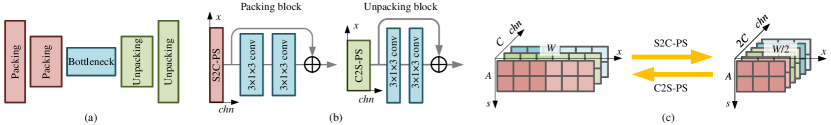
Figure 3: (a) An illustration of packing-unpacking network; (b) The packing block for the encoder (left) and the unpacking block decoder (right); (b) An illustration of Spatial-to-Channel Pixel Shuffle (S2C-PS) and Channel-to-Spatial Pixel Shuffle (C2S-PS).

III-B2 Network architectures

The networks in our proposed framework can be split into three parts: an encoder that extract high-level but low resolution features from high (spatial) resolution input, a bottleneck that performs non-linear mapping, and a decoder that restore high resolution target, i.e., a LF or a slice of the reconstruction cost volume, from high-level low resolution features. Table I lists the detail configurations of the NI and DIBR networks. The encoders and decoders of the NI and DIBR networks incorporate two packing-unpacking blocks symmetrically. We use a fold factor of 2 for each packing block and a fold factor of $1/2$ for each unpacking block. In the tables, we term the fold factor as stride factor for the convenience. For each residual module in the packing/unpacking block, we apply leaky ReLU activation after the first convolutional layers.

TABLE I: Detail configuration of the proposed NI network, where $k$ denotes the kernel size, $s$ the stride, Conv the 3D convolution layer, Deconv the 3D deconvolution layer and $\oplus$ the element-wise addition. $A^{\prime}=\alpha(A-1)+1$ is the angular resolution of the output LF. We ignore the batch dimension of tensors here.

Layer	$k$	$s$	Output Dim.
Encoder
Conv1	[3, 3, 3]	[1, 1, 1]	$W\times H\times A_{1}\times 16$
Pack.1	-	[2, 1, 1]	$W/2\times H\times A_{1}\times 32$
Pack.2	-	[2, 1, 1]	$W/4\times H\times A_{1}\times 64$
Bottleneck: $\times 1$ for NI network, $\times K$ for DIBR network
Conv2	[3, 1, 3]	[1, 1, 1]	$W/4\times H\times A_{1}\times 64$
Conv3	[3, 1, 3]	[1, 1, 1]	$W/4\times H\times A_{1}\times 64$
Conv3$\oplus$Pack.2	-	-	$W/4\times H\times A_{1}\times 64$
Reconstruction: $\times 1$ for NI network, $\times 0$ for DIBR network
DeConv	[5, 1, $2\alpha+1$]	[1, 1, $\frac{1}{\alpha}$]	$W/4\times H\times A_{2}\times 64$
Decoder
Unpack.1	-	[1/2, 1, 1]	$W/2\times H\times A_{2}\times 32$
Unpack.2	-	[1/2, 1, 1]	$W\times H\times A_{2}\times 16$
Conv5	[3, 3, 3]	[1, 1, 1]	$W\times H\times A_{2}\times 1$

The main difference between the NI and DIBR networks is as follows. For the NI network, we use one residual module ($K=1$) in the bottleneck. We insert a deconvolutional layer (also known as transposed convolution layer) of stride [1, 1, $1/\alpha$] at the end of the bottleneck to achieve plenoptic reconstruction. Thus, the angular resolutions of the output features are $A_{1}=A$ and $A_{2}=\alpha(A-1)+1$. For the DIBR network, we stack $K=2$ residual modules in the bottleneck. The angular resolutions of the output features are $A_{1}=A_{2}=\alpha(A-1)+1$.

III-B3 Discussions

In our practical implementation, we do not employ skip connections (like those in standard U-net [58]) to concatenate low-level features in the encoder with high-level features in the decoder. Because the residual modules [27] have already provided a path for the flow of information and gradients throughout the network. Please refer to Sec. IV-C for the comparison between the proposed packing-unpacking structure and standard U-net.

The inputs of the networks are 6 dimensional tensors of shape $D\times B\times W\times H\times A\times C$ (i.e., shear, batch, width, height, angular and channel). A straightforward implementation is to employ a network that is fully convolutional along the shear, width, height and angular dimensions. However, this architecture design will make the network parameters extremely large due to the requirement of 4D convolution. Fortunately, each slice $\mathcal{H}_{d}(L)$ in the reconstruction task (NI network) or $\tilde{L}_{d}$ in the cost assignment task (DIBR network) is independent along the shear dimension. Therefore, we can feed them to the networks slice by slice, i.e., $\mathcal{H}_{d}(L)$ or $\tilde{L}_{d}$. In our practice implementation, we employ a more efficient implementation by reshaping the network inputs into 5 dimensional tensors of shape $DB\times W\times H\times A\times C$. Then the reconstructed slices or the reconstruction cost volume can be inferred with a single forward-propagation.

III-C Implementation

III-C1 Training objective

In a narrow sense, the objectives between the NI and DIBR networks in our framework is different. The objective of the NI network is to reconstruct a high angular resolution LF. While the objective of the DIBR network is to evaluate whether the LF is well reconstructed under a certain depth hypothesis. The latter objective is hard to achieve when the ground truth depth is unavailable. Fortunately, from a macro perspective, the objective of the entire framework is to synthesize a high-quality LF. In addition, all modules in our framework are differentiable, and thus, the proposed Geo-NI framework can be trained in an end-to-end manner.

We measure the $L_{1}$ distance between the reconstructed light filed $\tilde{L}$ and the desired high angular resolution LF $L$ to optimize the parameters $\theta$ in the NI network, and the $L_{1}$ distance between the final output $\hat{L}$ and the desired LF $L$ to optimize the parameters $\vartheta$ in the DIBR network. The overall training objective is formulated as follows

$$\min_{\theta,\vartheta}\sum_{n}\|\tilde{L}^{(n)}_{d^{*}}-L^{(n)}\|_{1}+\|\hat{L}^{(n)}\odot\mathcal{M}-L^{(n)}\odot\mathcal{M}\|_{1},$$

where $\tilde{L}_{d^{*}}$ indicates the LF with shear amount $d=0$, $n$ denotes the $n^{\text{th}}$ training instance, $\mathcal{M}$ is a binary mask that avoids computing the loss on pixels that do not have valid values caused by the shearing operation and $\odot$ denotes element-wise multiplication.

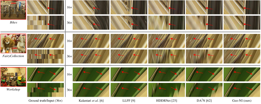
Figure 4: Comparison of the results (reconstructed EPIs) on LFs from the MPI Light Field Archive [15] (reconstruction scales $16\times$ and $36\times$). The second column shows the ground truth EPI and the input EPI for $36\times$ reconstruction.

III-C2 Training Data

We train the networks in the proposed Geo-NI framework by using LFs from the Stanford (New) Light Field Archive [59], which contains 12 LFs with $17\times 17$ views (the Lego Gantry Self Portrait is excluded due to the moving object in the scene). Since the network input is 3D LFs, we can extract 17 $L(x,y,s)$ and 17 $L(y,x,t)$ in each 4D LF set. To enhance the performance of the DIBR network, we augment the extracted 3D LFs using the shearing operation in Eqn. 1 with shear amounts $d=\pm 2$. This augmentation increases the number of training examples by 2 times. In the training procedure, we crop the extracted 3D LFs into sub-LFs with spatial resolution $128\times 18$ (width and height) and a stride of 40 pixels. We have three settings with respect to the reconstruction factors $\alpha=4,7$ in the NI network. Thus, the input/output angular resolution of the training samples for the Geo-NI framework are 5/17 and 3/15, respectively. Although the reconstruction factor of the network is fixed, we can achieve a flexible upsampling rate through network cascade.

III-C3 Training Details

In our implementation, the reconstruction is performed on the luminance channel (Y channel) in the YCbCr color space. The parameters in the networks are initialized with values drawn from the normal distribution (zero mean and standard deviation of $1\times 10^{-2}$). We optimize the networks by using ADAM solver [60] with learning rate of $1\times 10^{-4}$ ($\beta_{1}=0.9$, $\beta_{2}=0.999$) and mini-batch size of 8. The network converges after $200$ epochs on the training dataset. The proposed Geo-NI is implemented in the Pytorch framework [61].

IV Evaluations

In this section, we evaluate the proposed Geo-NI framework on various kinds of LFs, including those from both gantry systems and from plenoptic camera (Lytro Illum [50]). We mainly compare our method with two depth-based methods, Kalantari et al. [6] (depth-based) and LLFF [9] (MPI representation) and four depth-independent methods, Wu et al. [7], Yeung et al. [11], HDDRNet [26] and DA²N [62]. The quantitative evaluations is reported by measuring the average PSNR and SSIM [63] values over the synthesized views of the luminance channel in the YCbCr space. Please refer to the submitted video for more qualitative results.

Figure 5: Comparison of the results on LFs from the CIVIT Dataset [49] (reconstruction scales $16\times$ and $36\times$). The second column shows the ground truth EPI and the input EPI for $36\times$ reconstruction.

TABLE II: Quantitative results (PSNR/SSIM) of reconstructed light fields on LFs from the MPI Light Field Archive [15].

	Scale	Bikes	FairyCollection	LivingRoom	Mannequin	WorkShop	Average
Kalantari et al. [6]	$16\times$	30.67 / 0.935	32.39 / 0.952	41.62 / 0.973	37.15 / 0.970	33.94 / 0.971	35.15 / 0.960
Wu et al. [7]		31.22 / 0.951	30.33 / 0.942	42.43 / 0.991	39.53 / 0.989	33.49 / 0.977	35.40 / 0.970
Yeung et al. [11]		32.67 / 0.967	31.82 / 0.969	43.54 / 0.993	40.82 / 0.992	37.21 / 0.988	37.21 / 0.982
LLFF [9]		34.95 / 0.963	34.01 / 0.966	44.73 / 0.987	39.92 / 0.985	37.61 / 0.985	38.24 / 0.977
HDDRNet [26]		33.97 / 0.976	35.08 / 0.979	44.83 / 0.997	40.60 / 0.993	38.54 / 0.992	38.60 / 0.987
DA2N [62]		35.79 / 0.984	36.23 / 0.981	45.91 / 0.996	40.83 / 0.992	40.11 / 0.994	39.77 / 0.990
Geo-NI (NI only)		36.65 / 0.987	38.05 / 0.989	47.27 / 0.997	41.51 / 0.993	41.68 / 0.995	41.03 / 0.992
Geo-NI (bilinear)		34.02 / 0.980	34.96 / 0.985	39.89 / 0.993	37.59 / 0.989	36.04 / 0.989	36.50 / 0.987
Geo-NI (U-net)		35.07 / 0.980	38.25 / 0.987	45.77 / 0.995	41.17 / 0.992	39.25 / 0.993	39.90 / 0.990
Geo-NI (ours)		36.95 / 0.989	38.76 / 0.991	46.96 / 0.997	41.52 / 0.993	41.85 / 0.996	41.21 / 0.993
Kalantari et al. [6]	$36\times$	26.99 / 0.869	28.34 / 0.905	37.10 / 0.929	33.82 / 0.945	29.61 / 0.938	31.71 / 0.917
Wu et al. [7]		25.44 / 0.856	23.60 / 0.807	35.31 / 0.948	31.79 / 0.945	25.42 / 0.873	28.31 / 0.886
Yeung et al. [11]		26.92 / 0.896	27.12 / 0.897	37.44 / 0.970	33.77 / 0.963	28.70 / 0.932	30.79 / 0.932
LLFF [9]		27.40 / 0.892	28.56 / 0.918	39.54 / 0.980	33.53 / 0.949	30.12 / 0.949	31.83 / 0.938
HDDRNet [26]		26.35 / 0.886	24.50 / 0.853	36.17 / 0.966	32.47 / 0.960	27.16 / 0.919	29.33 / 0.917
DA2N [62]		27.94 / 0.917	26.52 / 0.903	38.39 / 0.975	35.70 / 0.976	29.80 / 0.961	30.67 / 0.932
Geo-NI (NI only)		27.86 / 0.916	27.58 / 0.921	41.22 / 0.988	35.11 / 0.974	31.54 / 0.972	32.66 / 0.954
Geo-NI (bilinear)		28.57 / 0.934	29.37 / 0.949	37.23 / 0.987	33.48 / 0.972	31.73 / 0.975	32.08 / 0.963
Geo-NI (U-net)		28.99 / 0.932	29.16 / 0.939	40.08 / 0.984	34.49 / 0.969	32.32 / 0.972	33.01 / 0.959
Geo-NI (ours)		30.00 / 0.950	31.13 / 0.961	43.02 / 0.993	35.36 / 0.976	34.37 / 0.984	34.78 / 0.973

IV-A Evaluations on Light Fields from Gantry Systems

IV-A1 Experiment settings

The comparisons are performed on 3D LFs from the MPI Light Field Archive [15] and the CIVIT Dataset [49]. The resolutions of the datasets are $960\times 720\times 101$ and $1280\times 720\times 193$ (width, height and angular). In this experiment, we use two upsampling scale settings to evaluate the capability of the proposed Geo-NI: $16\times$ reconstruction using 7/13 views as input (MPI Light Field Archive [15]/CIVIT Dataset [49]) and $36\times$ reconstruction using 3/6 views as input. The depth hypotheses $d\in D$ for the shearing operation are set to $\{0,\pm 4,\pm 8,\pm 12,\pm 16\}$ for $16\times$ reconstruction and $\{0,\pm 4,\pm 8,\pm 12,\pm 16,\pm 20,\pm 24,\pm 28\}$ for $36\times$ reconstruction, respectively.

Since the vanilla version of the network by Yeung et al. [11] and Meng et al. [26] (HDDRNet) were specifically designed for 4D LFs, we modify their convolutional layers to fit the 3D input while keeping its network architecture unchanged. We re-train the networks in the state-of-the-art methods (Kalantari et al. [6], Yeung et al. [11], LLFF [9] and HDDRNet [26] by using the same training dataset as the proposed Geo-NI. Due to the particularity of the training datasets, we compare DA²N [62] using the released network parameters. We perform network cascade to achieve different upsampling scales, i.e., two (three) cascades for $16\times$ ($36\times$) upsampling using a network of reconstruction factor $\alpha=4$.

TABLE III: Quantitative results (PSNR/SSIM) of reconstructed light fields on LFs from the CIVIT Dataset [49].

	Scale	Seal & Balls	Castle	Holiday	Dragon	Flowers	Average
Kalantari et al. [6]	$16\times$	43.13 / 0.985	36.03 / 0.965	32.44 / 0.961	39.50 / 0.985	35.21 / 0.973	37.26 / 0.974
Wu et al. [7]		45.21 / 0.994	35.20 / 0.977	35.58 / 0.987	46.39 / 0.997	41.60 / 0.995	40.80 / 0.990
Yeung et al. [11]		44.38 / 0.992	37.86 / 0.989	36.06 / 0.988	45.52 / 0.997	42.30 / 0.994	41.22 / 0.992
LLFF [9]		45.50 / 0.990	38.60 / 0.971	36.69 / 0.984	44.80 / 0.992	41.19 / 0.989	41.36 / 0.985
HDDRNet [26]		44.24 / 0.997	39.88 / 0.991	38.09 / 0.992	44.26 / 0.997	42.04 / 0.996	41.70 / 0.995
DA2N [62]		46.19 / 0.996	40.77 / 0.992	37.99 / 0.992	47.19 / 0.998	41.95 / 0.996	42.82 / 0.995
Geo-NI (NI only)		49.42 / 0.998	41.43 / 0.992	39.02 / 0.993	48.57 / 0.998	44.65 / 0.997	44.62 / 0.996
Geo-NI (bilinear)		39.43 / 0.995	38.30 / 0.990	34.70 / 0.987	39.82 / 0.997	38.48 / 0.994	38.15 / 0.993
Geo-NI (U-net)		47.72 / 0.997	41.26 / 0.992	38.21 / 0.991	47.85 / 0.997	42.19 / 0.995	43.44 / 0.995
Geo-NI (ours)		49.25 / 0.998	41.50 / 0.993	39.12 / 0.993	48.58 / 0.998	44.73 / 0.997	44.63 / 0.996
Kalantari et al. [6]	$36\times$	38.01 / 0.977	32.95 / 0.948	29.11 / 0.928	35.49 / 0.975	32.51 / 0.959	33.61 / 0.957
Wu et al. [7]		37.34 / 0.969	31.15 / 0.960	27.99 / 0.927	33.77 / 0.974	34.02 / 0.977	32.54 / 0.961
Yeung et al. [11]		38.56 / 0.979	33.12 / 0.971	29.97 / 0.952	36.95 / 0.986	34.93 / 0.982	34.71 / 0.974
LLFF [9]		40.55 / 0.982	33.95 / 0.954	30.16 / 0.941	37.99 / 0.980	33.50 / 0.969	35.23 / 0.965
HDDRNet [26]		40.15 / 0.984	33.35 / 0.972	30.62 / 0.957	35.83 / 0.985	36.76 / 0.988	35.34 / 0.977
DA2N [62]		43.96 / 0.992	36.58 / 0.983	32.78 / 0.973	43.61 / 0.996	36.67 / 0.988	38.72 / 0.986
Geo-NI (NI only)		44.23 / 0.993	36.75 / 0.985	32.72 / 0.974	43.66 / 0.996	37.54 / 0.990	38.98 / 0.987
Geo-NI (bilinear)		37.91 / 0.992	35.31 / 0.983	30.97 / 0.968	38.12 / 0.995	35.10 / 0.987	35.48 / 0.985
Geo-NI (U-net)		44.46 / 0.993	36.82 / 0.982	32.27 / 0.969	44.06 / 0.996	37.02 / 0.985	38.93 / 0.985
Geo-NI (ours)		45.78 / 0.996	37.50 / 0.987	32.96 / 0.976	45.39 / 0.997	38.36 / 0.991	40.00 / 0.990

IV-A2 Qualitative comparison

Fig. 4 shows three reconstruction results on LFs (Bikes, FairyCollection and WorkShop) from the MPI Light Field Archive [15]. And Fig. 5 shows the reconstruction results on LFs (Castle, Holiday and Flowers) from the CIVIT Dataset [49]. We demonstrate results with upsampling scale $16\times$ as well as $36\times$ on these two datasets. The maximum disparity range of the $36\times$ reconstruction reaches 75 pixels in the FairyCollection case [15].

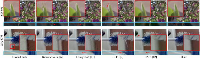
Figure 6: Comparison of the results on LFs from Lytro Illum. The results show the reconstructed views, zoom-in regions and the EPIs at the location marked by red lines. LFs are Flowers1 and IMG1743 from the 30 Scenes [6].

The qualitative comparisons indicate that the proposed Geo-NI framework is able to produce high-quality reconstruction on scenes with large disparities or non-Lambertian effects. The depth-based methods, Kalantari et al. [6] and LLFF [9], show high performance on simple structured scenes with large disparities while the depth-independent methods, HDDRNet [26] and DA²N [62], appear aliasing effects especially for $36\times$ reconstruction, e.g., the WorkShop case in Fig. 4. For scenes with complex structures or non-Lambertian effects but with relatively small disparities, the depth-independent methods, HDDRNet [26] and DA²N [62], outperforms the depth-based methods, Kalantari et al. [6] and LLFF [9], e.g., the cases Bikes and FairyCollection in Fig. 4 and the three cases in Fig. 5. However, the original structure or non-Lambertian effects will not be preserved in the results by the baseline methods when the input views are extremely sparse ($36\times$). The proposed Geo-NI is able to effectively combine the advantages of depth-based methods and depth-independent methods, and produces plausible reconstruction results on challenge cases with large disparities, complex structures or non-Lambertian effects.

IV-A3 Quantitative comparison

The quantitative results of $16\times$ and $36\times$ reconstructions for the MPI Light Field Archive [15] and the CIVIT Dataset [49] are shown in Table II and Table III, respectively. For LFs with relatively small disparities ($16\times$ reconstruction), the methods without any depth information by Wu et al. [7], Yeung et al. [11] and Meng et al. [26] (HDDRNet) is comparable to the depth-based methods by Kalantari et al. [6] and Mildenhall et al. [9] (LLFF). However, the performances of the depth-free methods drop quickly when the disparity is large. For example, on the CIVIT Dataset [49] (Table III), the PSNR of the method by Wu et al. [7] is 3dB higher than the method by Kalantari et al. [6] for $16\times$ reconstruction but 1dB lower for $36\times$ reconstruction. Compared with the baseline methods, the proposed Geo-NI framework shows superior performance on both LF datasets.

IV-B Evaluations on Light Fields from Lytro Illum

IV-B1 Experiment settings

The comparisons are performed on 4D LFs from three Lytro Illum datasets, the 30 Scenes dataset (30 LFs) by Kalantari et al. [6], and the Reflective (32 LFs) and Occlusions (51 LFs) categories from the Stanford Lytro Light Field Archive [64]. In this experiment, the upsampling factor is set to $7\times$ using $2\times 2$ views as input to reconstruct a $8\times 8$ LF. The depth hypotheses $d\in D$ for the shearing operation is set to $\{0,\pm 4,\pm 8,\pm 12,\pm 16\}$.

In addition to the methods evaluated in Sec. IV-A, we also compare the proposed Geo-NI framework with a depth-based method by Meng et al. [44]. Since the vanilla versions of the networks in [6, 11, 21, 26, 44] are trained on Lytro LFs, we use their released network parameters without re-training. The networks by Wu et al. [7] and Mildenhall et al. [9] (LLFF) are re-trained using the same dataset introduced in Sec. III-C2.

TABLE IV: Quantitative results (PSNR/SSIM) of reconstructed views on LFs from Lytro Illum [50] ($7\times$ reconstruction, $2\times 2\rightarrow 8\times 8$).

	30 Scenes [6]	Reflective [64]	Occlusions [64]
Kalantari et al. [6]	38.21 / 0.974	35.84 / 0.942	31.81 / 0.895
Wu et al. [7]	36.28 / 0.965	36.48 / 0.962	32.19 / 0.907
Yeung et al. [11]	39.22 / 0.977	36.47 / 0.947	32.68 / 0.906
LLFF [9]	38.17 / 0.974	36.40 / 0.948	31.96 / 0.901
HDDRNet [26]	38.33 / 0.967	36.77 / 0.931	32.78 / 0.909
Meng et al. [44]	39.14 / 0.970	37.01 / 0.950	33.10 / 0.912
DA2N [62]	38.99 / 0.986	36.72 / 0.975	33.14 / 0.950
Geo-NI (NI only)	36.15 / 0.957	37.43 / 0.973	32.12 / 0.932
Geo-NI (bilinear)	40.28 / 0.990	37.44 / 0.976	34.35 / 0.965
Geo-NI (U-net)	39.96 / 0.988	37.18 / 0.974	33.59 / 0.957
Geo-NI (ours)	40.68 / 0.990	38.05 / 0.977	34.54 / 0.964

IV-B2 Qualitative comparison

Fig. 6 shows two results for $7\times$ reconstruction ($2\times 2\rightarrow 8\times 8$) on LFs (Flower1 and IMG1743) from the 30 Scenes [6]. In the IMG1743 case, the maximum disparity reaches about 26 pixels between input views.

In the first case, the depth-independent methods by Yeung et al. [11] and DA²N [62] produce promising results due to the relatively small disparities. While the depth-base methods by Kalantari et al. [6] and LLFF [9] produce ghosting or tearing artifacts around occlusion boundaries. In the second case, the result by Yeung et al. [11] appears aliasing effects in the background due to the large disparity. While the DA²N [62] network generates blurry result as shown by the background door in the zoom-in figure and EPI. For the depth-based methods, the networks by Kalantari et al. [6] produce sever aliasing effects due to errors in depth estimation. The MPI-based method, LLFF [9], shows plausible result in the second case. However, the plane assignment error introduces tearing artifacts in the rendered view, as shown by the zoom-in figure. In comparison, the proposed Geo-NI framework provides reconstructed LFs with higher view consistency (as shown in the demonstrated EPIs).

IV-B3 Quantitative comparison

Table IV lists the quantitative results (PSNR/SSIM) averaged on LFs in each dataset. Limited by the baseline between viewpoints, the disparity range of LFs from Lytro Illum is smaller than that from gantry system, despite we only sample two viewpoints in each angular dimension, i.e., generally smaller than 14 pixels. Therefore, the depth-independent methods are able to achieve comparable or even superior performances than the depth-based methods. Since the DIBR network is able to elaborately select LFs with the highest reconstruction quality, the proposed Geo-NI achieves the highest PSNR and SSIM values among the depth-based and depth-independent methods.

IV-C Ablation studies

In this subsection, we empirically investigate the modules in the proposed Geo-NI framework by performing the following ablation studies.

Figure 7: The performance (PSNR) of the Geo-NI framework for different downsampling scales vs. different settings of shear range. Each grid shows the PSNR value (averaged on LFs from the MPI Light Field Archive [15]) of a certain downsampling scale under a certain setting of shear range.

IV-C1 Shear range

We investigate the capability of the Geo-NI framework under different settings of shear range (range of shear amounts). We implement this experiment by evaluating the performance of the Geo-NI under different downsampling scales when choosing different ranges of shear amounts (depth hypotheses), where different downsampling scales will lead to different disparity ranges in the input LF. The result (evaluated on the MPI Light Field Archive [15]) is plotted in Fig. 7, where the horizontal axis denotes the downsampling scale and the vertical axis the shear range. The shear values are evenly sampled every 4 pixels within the range. The result shows that the proposed Geo-NI is able to achieve a high-quality reconstruction when a reasonable shear range is provided. For instance, for the donwnsampling scale 48, the disparity range averaged on the test LFs is around $[-30,35]$, the Geo-NI provides the best reconstruction results when the shear range is set to $[-32,32]$ or $[-40,40]$. In addition, the result also indicates that the Geo-NI is robust to the settings of shear range. For example, for the donwnsampling scale 32 (averaged disparity range $[-20,23]$), the quantitative result varies from 35.49dB to 35.53dB (0.04dB gap) when we set the shear range from $[-24,24]$ or $[-48,48]$. Therefore, the proposed Geo-NI is able to generate satisfactory results even when an optimal shear range is not provided.

IV-C2 Neural interpolation only

This setting demonstrates the effectiveness of the DIBR part by detaching all components behind the NI network, which also equals to setting the depth hypotheses to zeros. We term this setting as “Geo-NI (NI only)” for short. As shown by the results in Table II, III and IV, without using the proposed DIBR part, the Geo-NI (NI only) is able to perform high-quality reconstruction at small downsampling scale (please refer to results of $16\times$ reconstruction in Table II, III), even achieving the highest PSNR value on cases LivingRoom [15] and Seal & Balls [49]. But the performances deceases significantly when the input LFs become sparser, e.g., the PSNR decreases 2dB for $36\times$ reconstruction on LFs from the MPI Light Field Archive [15]. On the other hand, it also indicates that the Geo-NI framework is able to enhance the performance of the NI network for LFs with large disparities via the selection of a proper shear amount.

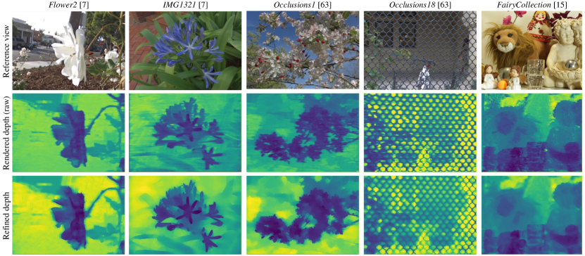
Figure 8: Illustration of rendered depth maps using reconstruction cost volumes produced by the DIBR network. The middle row shows the depth maps rendered from the raw reconstruction cost volumes. The last row shows the refined depth maps using the classical cost volume filtering method in [65].

IV-C3 Geo-NI with bilinear interpolation

In this experiment, we replace the NI network with a simple bilinear interpolation, denoted as “Geo-NI (bilinear)” for short. Benefiting from the perception of scene geometry in the DIBR part, the Geo-NI outperforms the most baseline methods at large downsampling scale (please refer to results of $36\times$ reconstruction in Table II, III and $7\times$ reconstruction in Table IV), despite it does not use a powerful neural network for LF reconstruction. This ablation study further illustrates the efficacy of the DIBR part in the proposed Geo-NI framework.

IV-C4 Packing-unpacking structure

We validate the effectiveness of the proposed packing-unpacking structure by replacing it with a typical 3D U-net, denoted as “Geo-NI (U-net)” for short. Specifically, we discard the S2C-PS (C2S-PS) operations in the packing (unpacking) blocks, and use convolution (deconvolution) layers with stride 2 ($1/2$) to compress (restore) the spatial information. We also use skip connections between the encoder and decoder instead of those in the residual blocks to transmit the high frequency components. The dimensions of the network parameters are kept the same to the packing-unpacking network. As shown by the quantitative results listed in Table II, III and IV, the Geo-NI (U-net) also achieves a considerable performance with the help of the aliasing measurement mechanism in the DIBR part. However, the Geo-NI with U-net suffers from performance degradation compared with the complete structure, which demonstrates the effectiveness of the packing-unpacking structure.

V Further Analysis

In this section, we first introduce the byproduct of the proposed Geo-NI framework, i.e., depth rendering using reconstruction cost volume, then analyse the relation to conventional DIBR and learning-based DIBR.

V-A Depth Map Rendering

The reconstruction cost in the DIBR network implicitly selects a proper shear amount (i.e., depth value) from the hypotheses, which is essentially similar with the purpose of matching cost. Therefore, the DIBR network, to some extent, can be interpreted as a depth estimator. In a standard depth estimation pipeline, the initial depth map can be extracted from the cost volume using the WTA strategy [29], i.e., $\mathop{\arg\min}_{d\in D}\mathcal{C}_{d}$. However, this strategy is not able to regress a smooth disparity estimate. In our implementation, we use the soft argmin operation introduced by Kendall et al. [36] to extract the depth information $\mathcal{D}$ as

$$\mathcal{D}(x,y,s)=\sum_{d\in D}d\cdot\sigma_{d}(-\mathcal{C}_{d}(x,y,s)).$$ (3)

It should be noted that the extracted depth $\mathcal{D}$ is a 3D tensor indicating the variation along the angular dimension.

Fig. 8 shows the rendered depth by using the reconstruction cost volume in the proposed Geo-NI framework. The second and the last rows demonstrate depth maps rendered by using the raw reconstruction cost volumes and the filtered volumes using the classical cost volume filtering method proposed by Hosni et al. in [65]. The proposed Geo-NI is able to perceive the occlusion boundary despite the training objective of the networks is only LF rendering, as shown by the cases Occlusion1 and Occlusion18 in Fig. 8.

V-B Relation to Depth-Image-based Rendering

V-B1 Relation to conventional DIBR

Conventional DIBR methods first estimate the depth of the scene, then blend the warped views based on the scene geometry (depth). For the depth estimation, these methods typically construct a cost volume that records the matching cost of each pixel along the dimension of depth hypothesis. The depth of the scene is solved from the cost volume using Winner Takes All (WTA) strategy [29], e.g., argmin operation. Instead of focusing on solving the depth, our idea is to render the desired LF directly from the cost volume.

But conventional cost volume in DIBR has following problems to reach our idea: i) The cost measures the correspondence between features, it cannot be used to synthesis novel views straightforwardly; ii) The cost is usually aggregated along the angular dimension, leading to dimension mismatching with the LF data. We address these problems by measuring the aliasing effects of the sheared LFs in replacing of the correspondences of a single view. On the one hand, measuring the aliasing effect in the DIBR network helps to guarantee the photo-consistency for Lambertian regions with large disparities, as shown in Fig. 9 (black arrow). On the other hand, it preserves the non-Lambertian effect reconstructed by the NI network since there is no assumption of depth consistency along the angular dimension, as shown in Fig. 9 (red arrow).

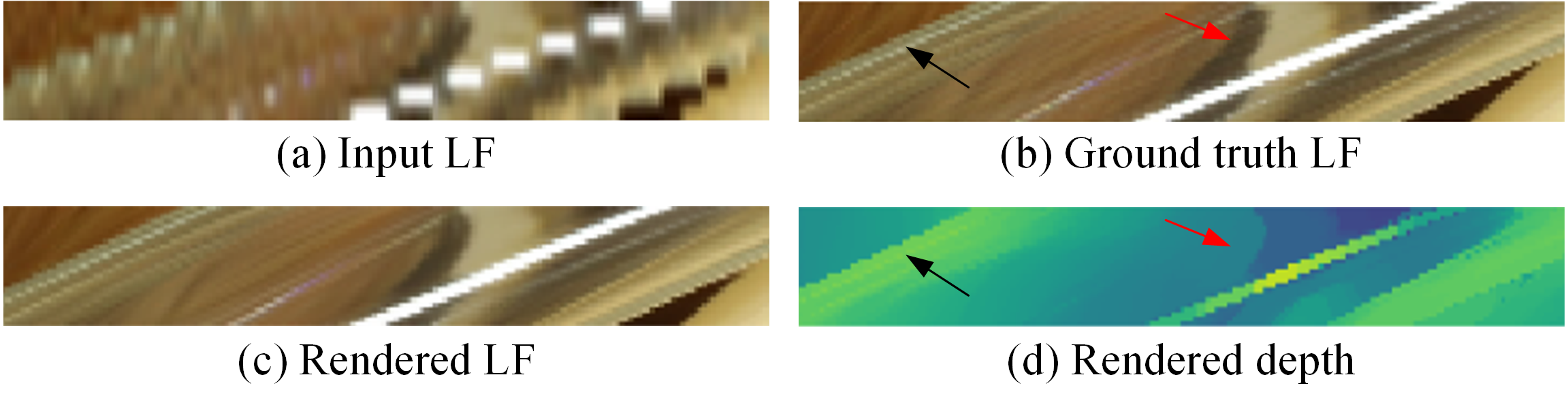
Figure 9: Measuring the aliasing effect in the reconstructed LF instead of the correspondence in standard cost volume helps to guarantee the photo-consistency for Lambertian regions with large disparities (as shown by the black arrow) as well as the non-Lambertian effect (as shown by the regions around the red arrow).

V-B2 Relation to learning-based DIBR

Standard learning-based DIBR methods [6, 43, 45, 46, 41] first estimate depth or optical flow via a neural network, and then refine the warped views or feature maps through another network to synthesize the novel view. The refinement network serves to correct the warping errors caused by the depth (flow) estimation network. However, when a region deviates too far from its proper position and the refinement network does not have a large enough receptive field, it will not be corrected. In comparison, the depth perception in the Geo-NI is moved to the rear part of the framework. For regions with small disparities and non-Lambertian effects, the NI network will yield good enough results. For regions with large disparities, the DIBR network is able to select high-quality reconstructed LFs under a certain shear amount through the lens of aliasing.

V-B3 Relation to reconstruction without implicit depth

In our previous works [66, 62], we use a similar strategy that deploys sheared LFs or EPIs in learning-based methods. However, the concept in this paper is fundamentally different. First, in the proposed framework, we elaborately implant NI within the DIBR pipeline. While in [62], a fusion network is applied to directly blend the sheared EPIs without utilizing the concept of DIBR. The DIBR pipeline in the proposed framework is able to turn the deep neural network into a white box by explaining how the network weights each slice of sheared LF using reconstruction cost. Second, all the modules in our framework is differentiable, ensuring the end-to-end optimization. In contrast, the method in [66] uses non-differentiable post-processing to reconstruct the high-angular resolution LF. Third, the method in [66] requires depth propagation between views before the reconstruction. In the proposed Geo-NI framework, we measure the aliasing effects of the neural interpolated LFs to generate a 3D depth volume (as described in Eqn. 3) rather than a single view, which guarantees the view consistency in the rendered LFs.

VI Conclusions

We have proposed a geometry-aware neural interpolation by launching a Neural Interpolation (NI) network within a Depth Image-Based Rendering (DIBR) pipeline. The NI network serves to reconstruct high angular resolution LFs which are sheared under a set of depth hypotheses. And the DIBR network is developed to construct a reconstruction cost volume through measuring the degrees of aliasing in the neural interpolated LFs, which is then applied for rendering the final LF. We have shown that the reconstruction cost volume in the DIBR network can be used to render scene depth of each view in the LFs. In addition, since we do not compel depth consistency between views, non-Lambertian effects reconstructed by the NI network can be maintained. For the NI and DIBR networks, we have designed a hierarchical packing-unpacking structure that effectively encodes and decodes LF features via spatial-channel pixel shuffling. Evaluations on various LF datasets have demonstrated that the combination of NI and DIBR pipeline is able to render high-quality LFs with large disparities and non-Lambertian effects.

Gaochang Wu received the BE and MS degrees in mechanical engineering in Northeastern University, Shenyang, China, in 2013 and 2015, respectively, and Ph.D. degree in control theory and control engineering in Northeastern University, Shenyang, China in 2020. He is currently an associate professor in the State Key Laboratory of Synthetical Automation for Process Industries, Northeastern University. His current research interests include image processing, light field processing and deep learning.

Yuemei Zhou received the B.E. degree from Beihang University (BUAA), Beijing, China, in 2018. She is currently pursuing the Ph.D. degree with the Department of Automation, Tsinghua University. Her research interests include image synthesis, image super-resolution and computational photography.

Yebin Liu received the BE degree from Beijing University of Posts and Telecommunications, China, in 2002, and the PhD degree from the Automation Department, Tsinghua University, Beijing, China, in 2009. He has been working as a research fellow at the computer graphics group of the Max Planck Institute for Informatik, Germany, in 2010. He is currently an associate professor in Tsinghua University. His research areas include computer vision and computer graphics.

Lu FANG is currently an Associate Professor at Tsinghua University. She received her Ph.D in Electronic and Computer Engineering from HKUST in 2011, and B.E. from USTC in 2007, respectively. Dr. Fang’s research interests include image / video processing, vision for intelligent robot, and computational photography. Dr. Fang serves as TC member in Multimedia Signal Processing Technical Committee (MMSP-TC) in IEEE Signal Processing Society.

Tianyou Chai received the Ph.D. degree in control theory and engineering from Northeastern University, Shenyang, China, in 1985. He has been with the Research Center of Automation, Northeastern University, Shenyang, China, since 1985, where he became a Professor in 1988 and a Chair Professor in 2004. His current research interests include adaptive control, intelligent decoupling control, integrated plant control and systems, and the development of control technologies with applications to various industrial processes. Prof. Chai is a member of the Chinese Academy of Engineering, an academician of International Eurasian Academy of Sciences, IEEE Fellow and IFAC Fellow. He is a distinguished visiting fellow of The Royal Academy of Engineering (UK) and an Invitation Fellow of Japan Society for the Promotion of Science (JSPS).

References

- [1] M. Levoy and P. Hanrahan, “Light field rendering,” in SIGGRAPH, 1996, pp. 31–42.
- [2] S. J. Gortler, R. Grzeszczuk, R. Szeliski, and M. F. Cohen, “The lumigraph,” in Siggraph, vol. 96, no. 30, 1996, pp. 43–54.
- [3] Z. Lin and H.-Y. Shum, “A geometric analysis of light field rendering,” International Journal of Computer Vision, vol. 58, no. 2, pp. 121–138, 2004.
- [4] G. Wu, B. Masia, A. Jarabo, Y. Zhang, L. Wang, Q. Dai, T. Chai, and Y. Liu, “Light field image processing: An overview,” IEEE JSTSP, vol. 11, no. 7, pp. 926–954, 2017.
- [5] D. Silver, J. Schrittwieser, K. Simonyan, I. Antonoglou, A. Huang, and e. a. Arthur Guez, “Mastering the game of go without human knowledge,” Nature, vol. 550, no. 7676, pp. 354–359, 2017.
- [6] N. K. Kalantari, T.-C. Wang, and R. Ramamoorthi, “Learning-based view synthesis for light field cameras,” ACM TOG, vol. 35, no. 6, 2016.
- [7] G. Wu, Y. Liu, L. Fang, Q. Dai, and T. Chai, “Light field reconstruction using convolutional network on epi and extended applications,” IEEE Transactions on Pattern Analysis and Machine Intelligence, vol. 41, no. 7, pp. 1681–1694, 2019.
- [8] R. S. Overbeck, D. Erickson, D. Evangelakos, M. Pharr, and P. Debevec, “A system for acquiring, processing, and rendering panoramic light field stills for virtual reality,” in SIGGRAPH, 2019, pp. 1–15.
- [9] B. Mildenhall, P. P. Srinivasan, R. Ortiz-Cayon, N. K. Kalantari, R. Ramamoorthi, R. Ng, and A. Kar, “Local light field fusion: Practical view synthesis with prescriptive sampling guidelines,” ACM Transactions on Graphics (TOG), vol. 38, no. 4, pp. 1–14, 2019.
- [10] Y. Yoon, H.-G. Jeon, D. Yoo, J.-Y. Lee, and I. So Kweon, “Learning a deep convolutional network for light-field image super-resolution,” in CVPRW, 2015, pp. 24–32.
- [11] H. W. F. Yeung, J. Hou, J. Chen, Y. Y. Chung, and X. Chen, “Fast light field reconstruction with deep coarse-to-fine modeling of spatial-angular clues,” in ECCV, 2018, pp. 138–154.
- [12] J. Long, Z. Ning, and T. Darrell, “Do convnets learn correspondence?” Advances in Neural Information Processing Systems, vol. 2, pp. 1601–1609, 2014.
- [13] B. Zhou, A. Khosla, A. Lapedriza, A. Oliva, and A. Torralba, “Object detectors emerge in deep scene cnns,” in International Conference on Learning Representations, 2015.
- [14] J. Jin, J. Hou, J. Chen, S. Kwong, and J. Yu, “Light field super-resolution via attention-guided fusion of hybrid lenses,” in Proceedings of the 28th ACM International Conference on Multimedia, 2020, pp. 193–201.
- [15] V. K. Adhikarla, M. Vinkler, D. Sumin, R. K. Mantiuk, K. Myszkowski, H.-P. Seidel, and P. Didyk, “Towards a quality metric for dense light fields,” in Proceedings of the IEEE Conference on Computer Vision and Pattern Recognition, 2017, pp. 58–67.
- [16] J.-X. Chai, X. Tong, S.-C. Chan, and H.-Y. Shum, “Plenoptic sampling,” in Proceedings of the 27th annual conference on Computer graphics and interactive techniques. ACM Press/Addison-Wesley Publishing Co., 2000, pp. 307–318.
- [17] C. Zhang and T. Chen, “Spectral analysis for sampling image-based rendering data,” IEEE Transactions on Circuits and Systems for Video Technology, vol. 13, no. 11, pp. 1038–1050, 2003.
- [18] S. Vagharshakyan, R. Bregovic, and A. Gotchev, “Light field reconstruction using shearlet transform,” IEEE TPAMI, vol. 40, no. 1, pp. 133–147, 2018.
- [19] C. Zhu, H. Zhang, Q. Liu, Z. Zhuang, and L. Yu, “A signal-processing framework for occlusion of 3D scene to improve the rendering quality of views,” IEEE Transactions on Image Processing, vol. 29, pp. 8944–8959, 2020.
- [20] H. Zhu, M. Guo, H. Li, Q. Wang, and A. Robleskelly, “Revisiting spatio-angular trade-off in light field cameras and extended applications in super-resolution,” IEEE Transactions on Visualization and Computer Graphics, pp. 1–15, 2019.
- [21] Y. Wang, F. Liu, K. Zhang, Z. Wang, Z. Sun, and T. Tan, “High-fidelity view synthesis for light field imaging with extended pseudo 4DCNN,” IEEE Transactions on Computational Imaging, vol. 6, pp. 830–842, 2020.
- [22] Y. Wang, L. Wang, G. Wu, J. Yang, W. An, J. Yu, and Y. Guo, “Disentangling light fields for super-resolution and disparity estimation.” IEEE Transactions on Pattern Analysis and Machine Intelligence, pp. 1–1, 2021.
- [23] X. Shi, Z. Chen, H. Wang, D. Yeung, W. Wong, and W. Woo, “Convolutional lstm network: a machine learning approach for precipitation nowcasting,” in NIPS, 2015, pp. 802–810.
- [24] D. Liu, Y. Huang, Q. Wu, R. Ma, and P. An, “Multi-angular epipolar geometry based light field angular reconstruction network,” IEEE Transactions on Computational Imaging, vol. 6, pp. 1507–1522, 2020.
- [25] S. Zhang, S. Chang, Z. Shen, and Y. Lin, “Micro-lens image stack upsampling for densely-sampled light field reconstruction,” IEEE Transactions on Computational Imaging, vol. 7, pp. 799–811, 2021.
- [26] N. Meng, H. K.-H. So, X. Sun, and E. Y. Lam, “High-dimensional dense residual convolutional neural network for light field reconstruction,” IEEE Transactions on Pattern Analysis and Machine Intelligence, vol. 43, no. 3, pp. 873–886, 2021.
- [27] K. He, X. Zhang, S. Ren, and J. Sun, “Deep residual learning for image recognition,” in 2016 IEEE Conference on Computer Vision and Pattern Recognition (CVPR), 2016, pp. 770–778.
- [28] G. Huang, Z. Liu, L. van der Maaten, and K. Q. Weinberger, “Densely connected convolutional networks,” in IEEE Conference on Computer Vision and Pattern Recognition (CVPR), 2017, pp. 4700–4708.
- [29] D. Scharstein and R. Szeliski, “A taxonomy and evaluation of dense two-frame stereo correspondence algorithms,” International journal of computer vision, vol. 47, no. 1-3, pp. 7–42, 2002.
- [30] S. Wanner and B. Goldluecke, “Variational light field analysis for disparity estimation and super-resolution,” IEEE TPAMI, vol. 36, no. 3, pp. 606–619, 2014.
- [31] A. Vianello, J. Ackermann, M. Diebold, and B. Jähne, “Robust hough transform based 3d reconstruction from circular light fields,” in IEEE Conference on Computer Vision and Pattern Recognition, 2018, pp. 7327–7335.
- [32] C.-T. Huang, “Robust pseudo random fields for light-field stereo matching,” in Proceedings of the IEEE International Conference on Computer Vision, 2017, pp. 11–19.
- [33] M. W. Tao, S. Hadap, J. Malik, and R. Ramamoorthi, “Depth from combining defocus and correspondence using light-field cameras,” in ICCV, 2013, pp. 673–680.
- [34] T.-C. Wang, A. A. Efros, and R. Ramamoorthi, “Occlusion-aware depth estimation using light-field cameras,” in ICCV, 2015, pp. 3487–3495.
- [35] S. Zhang, H. Sheng, C. Li, J. Zhang, and Z. Xiong, “Robust depth estimation for light field via spinning parallelogram operator,” Computer Vision and Image Understanding, vol. 145, pp. 148–159, 2016.
- [36] A. Kendall, H. Martirosyan, S. Dasgupta, P. Henry, R. Kennedy, A. Bachrach, and A. Bry, “End-to-end learning of geometry and context for deep stereo regression,” in Proceedings of the IEEE International Conference on Computer Vision, 2017, pp. 66–75.
- [37] Y.-J. Tsai, Y.-L. Liu, M. Ouhyoung, and Y.-Y. Chuang, “Attention-based view selection networks for light-field disparity estimation,” in Proceedings of AAAI Conference on Artificial Intelligence (AAAI), 2020, p. 1.
- [38] E. Penner and L. Zhang, “Soft 3D reconstruction for view synthesis,” ACM TOG, vol. 36, no. 6, p. 235, 2017.
- [39] K. Ko, Y. J. Koh, S. Chang, and C.-S. Kim, “Light field super-resolution via adaptive feature remixing,” IEEE Transactions on Image Processing, vol. 30, pp. 4114–4128, 2021.
- [40] Y. Zhou, G. Wu, Y. Fu, K. Li, and Y. Liu, “Cross-MPI: Cross-scale stereo for image super-resolution using multiplane images,” in IEEE Conference on Computer Vision and Pattern Recognition, 2021, pp. 14 842–14 851.
- [41] M. Guo, J. Jin, H. Liu, and J. Hou, “Learning dynamic interpolation for extremely sparse light fields with wide baselines,” in IEEE International Conference on Computer Vision (ICCV), October 2021, pp. 2450–2459.
- [42] J. Flynn, I. Neulander, J. Philbin, and N. Snavely, “Deepstereo: Learning to predict new views from the world’s imagery,” in CVPR, 2015.
- [43] J. Shi, X. Jiang, and C. Guillemot, “Learning fused pixel and feature-based view reconstructions for light fields,” in IEEE Conference on Computer Vision and Pattern Recognition, 2020.
- [44] N. Meng, K. Li, J. Liu, and E. Y. Lam, “Light field view synthesis via aperture disparity and warping confidence map,” IEEE Transactions on Image Processing, vol. 30, pp. 3908–3921, 2021.
- [45] J. Jin, J. Hou, H. Yuan, and S. Kwong, “Learning light field angular super-resolution via a geometry-aware network.” in Proceedings of the AAAI Conference on Artificial Intelligence, vol. 34, no. 7, 2020, pp. 11 141–11 148.
- [46] J. Jin, J. Hou, J. Chen, H. Zeng, S. Kwong, and J. Yu, “Deep coarse-to-fine dense light field reconstruction with flexible sampling and geometry-aware fusion.” IEEE Transactions on Pattern Analysis and Machine Intelligence, no. 1, pp. 1–1, 2020.
- [47] T. Zhou, R. Tucker, J. Flynn, G. Fyffe, and N. Snavely, “Stereo magnification: Learning view synthesis using multiplane images,” in SIGGRAPH, 2018.
- [48] J. Flynn, M. Broxton, P. Debevec, M. DuVall, G. Fyffe, R. Overbeck, N. Snavely, and R. Tucker, “Deepview: View synthesis with learned gradient descent,” in IEEE Conference on Computer Vision and Pattern Recognition, 2019, pp. 2367–2376.
- [49] S. Moreschini, F. Gama, R. Bregovic, and A. Gotchev, “Civit dataset: Horizontal-parallax-only densely-sampled light-fields,” https://civit.fi/densely-sampled-light-field-datasets/.
- [50] “Lytro.” https://www.lytro.com/.
- [51] R. Ng, M. Levoy, M. Brédif, G. Duval, M. Horowitz, and P. Hanrahan, “Light field photography with a hand-held plenoptic camera,” in Stanford University Computer Science Tech Report, 2005.
- [52] G. Eilertsen, J. Kronander, G. Denes, R. K. Mantiuk, and J. Unger, “Hdr image reconstruction from a single exposure using deep cnns,” Acm Transactions on Graphics, 2017.
- [53] Y. Tan, H. Zheng, Y. Zhu, X. Yuan, X. Lin, D. Brady, and L. Fang, “Crossnet++: Cross-scale large-parallax warping for reference-based super-resolution,” IEEE Transactions on Pattern Analysis and Machine Intelligence, vol. 43, no. 12, pp. 4291–4305, 2020.
- [54] R. Zhang, “Making convolutional networks shift-invariant again,” in International conference on machine learning (PMLR), 2019, pp. 7324–7334.
- [55] V. Guizilini, R. Ambrus, S. Pillai, A. Raventos, and A. Gaidon, “3d packing for self-supervised monocular depth estimation,” in IEEE Conference on Computer Vision and Pattern Recognition (CVPR), 2020, pp. 2485–2494.
- [56] S. Zheng, J. Lu, H. Zhao, X. Zhu, Z. Luo, Y. Wang, Y. Fu, J. Feng, T. Xiang, P. H. Torr, and L. Zhang, “Rethinking semantic segmentation from a sequence-to-sequence perspective with transformers,” in IEEE Conference on Computer Vision and Pattern Recognition (CVPR), 2021, pp. 6881–6890.
- [57] W. Shi, J. Caballero, F. Huszar, J. Totz, A. P. Aitken, R. Bishop, D. Rueckert, and Z. Wang, “Real-time single image and video super-resolution using an efficient sub-pixel convolutional neural network,” in IEEE Conference on Computer Vision and Pattern Recognition, 2016, pp. 1874–1883.
- [58] O. Ronneberger, P. Fischer, and T. Brox, “U-net: Convolutional networks for biomedical image segmentation,” in International Conference on Medical Image Computing and Computer-Assisted Intervention, 2015, pp. 234–241.
- [59] “Stanford (New) Light Field Archive.” http://lightfield.stanford.edu/lfs.html.
- [60] D. P. Kingma and J. Ba, “Adam: A method for stochastic optimization,” in International Conference on Learning Representations, 2015.
- [61] A. Paszke, S. Gross, F. Massa, A. Lerer, J. Bradbury, G. Chanan, T. Killeen, Z. Lin, N. Gimelshein, L. Antiga, A. Desmaison, A. Kopf, E. Yang, Z. DeVito, M. Raison, A. Tejani, S. Chilamkurthy, B. Steiner, L. Fang, J. Bai, and S. Chintala, “Pytorch: An imperative style, high-performance deep learning library,” in Advances in Neural Information Processing Systems, vol. 32, 2019, pp. 1–12.
- [62] G. Wu, Y. Liu, L. Fang, and T. Chai, “Revisiting light field rendering with deep anti-aliasing neural network.” IEEE Transactions on Pattern Analysis and Machine Intelligence, pp. 1–1, 2021.
- [63] Z. Wang, A. C. Bovik, H. R. Sheikh, and E. P. Simoncelli, “Image quality assessment: from error visibility to structural similarity,” IEEE TIP, vol. 13, no. 4, pp. 600–612, 2004.
- [64] “Stanford Lytro Light Field Archive.” http://lightfields.stanford.edu/.
- [65] A. Hosni, C. Rhemann, M. Bleyer, C. Rother, and M. Gelautz, “Fast cost-volume filtering for visual correspondence and beyond,” IEEE Transactions on Pattern Analysis and Machine Intelligence, vol. 35, no. 2, pp. 504–511, 2013.
- [66] G. Wu, Y. Liu, Q. Dai, and T. Chai, “Learning sheared epi structure for light field reconstruction,” IEEE Transactions on Image Processing, vol. 28, no. 7, pp. 3261–3273, 2019.