HORSES3D: a high-order discontinuous Galerkin solver for flow simulations and multi-physics applications

Abstract

We present the latest developments of our High-Order Spectral Element Solver (HORSES3D), an open source high-order discontinuous Galerkin framework, capable of solving a variety of flow applications, including compressible flows (with or without shocks), incompressible flows, various RANS and LES turbulence models, particle dynamics, multiphase flows, and aeroacoustics. We provide an overview of the high-order spatial discretisation (including energy/entropy stable schemes) and anisotropic p-adaptation capabilities. The solver is parallelised using MPI and OpenMP showing good scalability for up to 1000 processors. Temporal discretisations include explicit, implicit, multigrid, and dual time-stepping schemes with efficient preconditioners. Additionally, we facilitate meshing and simulating complex geometries through a mesh-free immersed boundary technique. We detail the available documentation and the test cases included in the GitHub repository.

PROGRAM SUMMARY

Program Title: HORSES3D
CPC Library link to program files: (to be added by Technical Editor)
Developer’s repository link: private GitHub repository.
Code Ocean capsule: (to be added by Technical Editor)
Licensing provisions: MIT
Programming language: Fortran 2008
External routines/libraries: METIS, MPI, HDF5, MKL, PETSc (all are optional).
Nature of problem: HORSES3D is a high-order discontinuous Galerkin framework, capable of solving a variety of flow applications, including compressible flows (with or without shocks), incompressible flows, various RANS and LES turbulence models, particle dynamics, multiphase flows, and aeroacoustics.
Solution method: high-order discontinuous Galerkin Spectral Element (DGSEM) and explicit/implicit time-steppers.
Additional comments including restrictions and unusual features: HORSES3D is a multiphysics environment where the compressible Navier-Stokes equations, the incompressible Navier–Stokes equations, the Cahn–Hilliard equation and entropy–stable variants are solved. Arbitrary high–order, p–anisotropic discretisations are used, including static and dynamic p–adaptation methods (feature-based and truncation error-based). Explicit and implicit time-steppers for steady and time-marching solutions are available, including efficient multigrid and preconditioners. Numerical and analytical Jacobian computations with a coloring algorithm have been implemented. Multiphase flows are solved using a diffuse interface model: Navier–Stokes/Cahn–Hilliard. Turbulent models implemented include RANS: Spalart-Allmaras and LES: Smagorinsky, Wale, Vreman; including wall models. Immersed boundary methods can be used, to avoid creating body fitted meshes. Acoustic propagation can be computed using Ffowcs-Williams and Hawkings models. HORSES3D supports curvilinear, hexahedral, conforming meshes in GMSH, HDF5 and SpecMesh/HOHQMesh format. A hybrid CPU-based parallelisation strategy (shared and distributed memory) with OpenMP and MPI is followed.

1 Introduction

To simulate and predict complex flows, the non-linear Navier-Stokes (NS) equations that govern fluid flow need to be solved numerically. Traditional simulation solvers that use low-order methods (order $\leq$ 2, for example, finite differences or finite volumes) have been widely adopted by industry and academia to simulate fluid flows, but have limitations when high accuracy is required [1]. Low-order numerical techniques (most commercial codes) suffer from non-negligible numerical errors (e.g., dissipative and dispersive errors) that can increase unphysical dissipation and dispersion of flow structures and provide unrealistic results.

An alternative, to low order solvers, is to employ high-order discretisations based on polynomial approximations of the solution. These methods are characterised by low numerical errors, and their ability to use mesh refinement through an increased number of mesh nodes (h-refinement) and/or polynomial enrichment (p-refinement) to achieve highly accurate solutions. Such high-order polynomial methods produce an exponential decay of the error for smooth solutions instead of the algebraic decay characteristic of low-order techniques.

Typical aircraft aerodynamic simulations require an order of 50 to 100M degrees of freedom ($dof$), if low-order methods are used. Using high-order methods, the overall number of $dof$ can be reduced for a desired level of accuracy. Given a numerical scheme, the numerical error $e$ is proportional to $(dof)^{P}$, where $P$ is the order, see [2]. To achieve similar errors (i.e. $e_{HO}\approx e_{LO}$) between high- ($HO$) and low-order ($LO$) methods, the high-order mesh may be coarsened following: $(dof)_{HO}=\exp(P_{LO}/P_{HO}.\log[(dof)_{LO}])$. Selecting $P_{LO}=2$ and $P_{HO}=5$, one finds for $(dof)_{LO}=100M$ a corresponding mesh size $(dof)_{HO}=1.6k$; that is, a factor of 60000 decrease in $dof$ for the same accuracy. Of course, this estimate is optimistic, since in reality small cells are required near walls to resolve boundary layers. Nevertheless, this estimate illustrates how high-order methods can enable simulations with fewer degrees of freedom (while maintaining accuracy). Additional accuracy can be achieved with a limited increase in cost, when using local anisotropic p-refinement (i.e. only particular mesh elements and directions use high-order polynomials), [3, 4, 5, 6].

High-order numerical methods of spectral type (order $>$ 2) were first developed in the 1970s (e.g., [7]) and have typically been perceived as accurate but expensive methods, with a lack of flexibility (for complex geometries) and robustness (tendency to crash) when applied to complex turbulent flows. Although widely adopted in academia and particularly for low Reynolds numbers during the 1980s and 90s, it was not until the 2000s that these became a realistic alternative to well-established low-order techniques (finite differences or finite volumes). One of the main reasons for the increasing acceptance has been the development of high-order discontinuous Galerkin (DG) variants that include interelement fluxes that enhance robustness (when compared to classic high-order continuous methods). DG has seen a remarkable recent increase in popularity in the last 10 years. DG methods were first developed by Reed $\&$ Hill in the framework of neutron transport equations [8], but remained unexploited until the late 1990s, when the method was generalised to convection-diffusion problems that are used to simulate fluid flows: see, e.g., [9, 10]. Today, DG methods have been used to solve a wide variety of flows, including incompressible, compressible, or multiphase flows, but still need developments to become accepted within the industry (e.g., increased speed and robustness for turbulent flows).

DG is paving its way towards industry through research centres. For example, Airbus, Dyson, McLaren F1 or Siemens-Gamesa have collaborated with our group in various European projects to evaluate high-order methods. In these projects, aeronautical European research centres (e.g., ONERA or DLR) were also involved. DG methods are relatively mature for aeronautical applications, but require further developments to be widely adopted by industry (not necessarily aeronautical).

In this work, we summarise the main features included in our high-order DG solver HORSES3D:

The work is structured as follows. In Sec. 2, we contextualise HORSES3D with a review of the main capabilities of available high-order academic solvers. The rest of the paper can be split in two parts. In the first part: Numerical Method (Sec. 3), we describe the original features of the solver that was first conceived to solve the compressible Navier-Stokes equations. This part includes meshing (Sec. 3.1), the compressible Navier-Stokes solver (Sec. 3.2), the discontinuous Galerkin spatial discretisation (Sec. 3.3), the possibility to include alternate physics (Sec. 3.4), the available energy/entropy stable formulations to enhance stability (Sec. 3.5), local spatial p-adaption (Sec. 3.6), the time advancement methods available (Sec. 3.7) and parallelisation benchmarks (Sec. 3.8).

In the second part: Multiphysics (Sec. 4), we detail the extended capabilities of HORSES3D , including turbulent modelling (Sec. 4.1), incompressible flows (Sec. 4.2), multiphase flows (Sec. 4.3), shock capturing (Sec. 4.4), particle dynamics (Sec. 4.5), aeroacoustics (Sec. 4.6) and immersed boundaries (Sec. 4.7).

2 Review of high-order solvers

A range of high-order academic solvers exist and are briefly summarised in Table 1, where we include their main capabilities. We provide references for each solver and outline here the capabilities of interest when compared to HORSES3D. This list is a non-exhaustive summary where we have not included commercial software. The table reflects that HORSES3D provides a unique set of capabilities to simulate complex flows.

	HORSES3D	Nek5000	Nektar++	Semtex	deal.II	Flexi/Fluxo	Trixi	PyFR
References		[11]	[12, 13]	[14]	[15]	[16, 17]	[18, 19]	[20]
Language	Fortran	Fortran	C++	C++	C++	Fortran	Julia	Python
Spatial discretisation	DG	CG	CG/DG	CG	CG/DG	DG	DG	FR
Incompressible	✓	✓	✗	✓	✓	✗	✗	✓
Compressible	✓	✗	✓	✗	✓	✓	✓	✓
Energy/Entropy stable	✓	✗	✗	✗	✗	✓	✓	✗
p-adaptation	✓	✓	✓	✗	✓	✓	✓	✓
Steady/Unsteady	S/U	U	U	U	S/U	U	U	S/U
LES	✓	✓	✓	✓	✓	✓	✓	✓
RANS	✓	✗	✗	✗	✗	✗	✗	✗
Multiphase	✓	✓	✗	✗	✓	✗	✗	✓
Shocks	✓	✗	✓	✗	✓	✓	✓	✓
Particles	✓	✓	✓	✓	✓	✗	✗	✗
Aeroacoustics	✓	✗	✓	✗	✓	✗	✓	✗
Immersed Boundaries	✓	✗	✓	✗	✗	✗	✗	✗

Table 1: Summary of high-order solvers and capabilities.

3 Numerical methods

HORSES3D is a Fortran 2003 object-oriented solver, originally developed to solve the compressible Navier-Stokes equations using DG discretisations and explicit time marching. In this section, we detail the compressible solver together with the spatial- and temporal-time advancement schemes.

3.1 Meshing and Post-processing

The solver supports curvilinear, hexahedral and conforming meshes in GMSH [21], HDF5[22] and SpecMesh/HOHQMesh [23] format. Linear meshes generated in Gambit, ICEM, or CGNS can be curved and converted to HDF5 using HOPR [24]. If the user prefers to avoid generating body fitted meshes, we provide a mesh-free immersed boundary capability, which is detailed in (Sec. 4.7).

Tecplot and Paraview [25, 26] can be used to post-process the results. We have developed a post-processing utility horses2plt that allows interpolating to homogeneous nodal points (from Gauss-Legendre or Gauss-Lobatto) and modifying the polynomial order for visualisation purposes. The tool also allows to extract derived variables, such as vorticity and Q-criterion (if gradients are enabled during the simulation) or Reynolds Stresses (if the statistics are enabled during the simulation).

3.2 Compressible Navier-Stokes

The 3D Navier-Stokes equations can be compactly written as

$$\bm{u}_{t}+\nabla\cdot\accentset{\,\leftrightarrow}{\mathbf{F}}_{e}=\nabla\cdot\accentset{\,\leftrightarrow}{\mathbf{F}}_{v},$$ (1)

where $\bm{u}$ is the state vector of conservative variables $\bm{u}=[\rho,\rho v_{1},\rho v_{2},\rho v_{3},\rho e]^{T}$, $\accentset{\,\leftrightarrow}{\mathbf{F}}_{e}$ are the inviscid, or Euler fluxes,

$$\accentset{\,\leftrightarrow}{\mathbf{F}}_{e}=\left[\begin{array}[]{ccc}\rho v_{1}&\rho v_{2}&\rho u_{3}\\ \rho v_{1}^{2}+p&\rho v_{1}v_{2}&\rho v_{1}v_{3}\\ \rho v_{1}v_{2}&\rho v_{2}^{2}+p&\rho v_{2}v_{3}\\ \rho v_{1}v_{3}&\rho v_{2}v_{3}&\rho v_{3}^{2}+p\\ \rho v_{1}H&\rho v_{2}H&\rho v_{3}H\end{array}\right],$$ (2)

where $\rho$, $e$, $H=E+p/\rho$, and $p$ are the density, total energy, total enthalpy and pressure, respectively, and $\vec{v}=[v_{1},v_{2},v_{3}]^{T}$ is the velocity. Additionally, $\accentset{\,\leftrightarrow}{\mathbf{F}}_{v}$ defines the viscous fluxes,

$$\accentset{\,\leftrightarrow}{\mathbf{F}}_{v}=\left[\begin{array}[]{ccc}0&0&0\\ \tau_{xx}&\tau_{xy}&\tau_{xz}\\ \tau_{yx}&\tau_{yy}&\tau_{yz}\\ \tau_{zx}&\tau_{zy}&\tau_{zz}\\ \sum_{j=1}^{3}v_{j}\tau_{1j}+\kappa T_{x}&\sum_{j=1}^{3}v_{j}\tau_{2j}+\kappa T_{y}&\sum_{j=1}^{3}v_{j}\tau_{3j}+\kappa T_{z}\end{array}\right],$$ (3)

where $\kappa$ is the thermal conductivity, $T_{x},T_{y}$ and $T_{z}$ denote the temperature gradients and the stress tensor $\bm{\tau}$ is defined as $\bm{\tau}=\mu(\nabla\vec{v}+(\nabla\vec{v})^{T})-2/3\mu\bm{I}\nabla\cdot\vec{v}$, with $\mu$ the dynamic viscosity and $\bm{I}$ the three-dimensional identity matrix.

3.3 Spatial discretisation: discontinuous Galerkin

HORSES3D discretises the Navier-Stokes equations using the Discontinuous Galerkin Spectral Element Method (DGSEM), which is a particularly efficient nodal version of DG schemes [27]. For simplicity, here we only introduce the fundamental concepts of DG discretisations. More details can be found in [28, 29].

The physical domain is tessellated with non-overlapping curvilinear hexahedral elements, $e$, which are geometrically transformed to a reference element, $el$. This transformation is performed using a polynomial transfinite mapping that relates the physical coordinates $\vec{x}$ and the local reference coordinates $\vec{\xi}$. The transformation is applied to (1) resulting in the following:

$$J\bm{u}_{t}+\nabla_{\xi}\cdot\accentset{\,\leftrightarrow}{\tilde{\mathbf{F}}}_{e}=\nabla_{\xi}\cdot\accentset{\,\leftrightarrow}{\tilde{\mathbf{F}}}_{v},$$ (4)

where $J$ is the Jacobian of the transfinite mapping, $\nabla_{\xi}$ is the differential operator in the reference space and $\accentset{\,\leftrightarrow}{\tilde{\mathbf{F}}}$ are the contravariant fluxes [27].

To derive DG schemes, we multiply (4) by a locally smooth test function $\phi_{j}$, for $0\leq j\leq P$, where $P$ is the polynomial degree, and integrate over an element $el$ to obtain the weak form

$$\int_{el}J\bm{u}_{t}\phi_{j}+\int_{el}\nabla_{\xi}\cdot\accentset{\,\leftrightarrow}{\tilde{\mathbf{F}}}_{e}\phi_{j}=\int_{el}\nabla_{\xi}\cdot\accentset{\,\leftrightarrow}{\tilde{\mathbf{F}}}_{v}\phi_{j}.$$ (5)

We can now integrate by parts the term with the inviscid fluxes, $\accentset{\,\leftrightarrow}{\tilde{\mathbf{F}}}_{e}$, to obtain a local weak form of the equations (one per mesh element) with the boundary fluxes separated from the interior

$$\int_{el}J\bm{u}_{t}\phi_{j}+\int_{\partial el}\accentset{\,\leftrightarrow}{\tilde{\mathbf{F}}}_{e}\cdot\hat{\mathbf{n}}\phi_{j}-\int_{el}\accentset{\,\leftrightarrow}{\tilde{\mathbf{F}}}_{e}\cdot\nabla_{\xi}\phi_{j}=\int_{el}\nabla_{\xi}\cdot\accentset{\,\leftrightarrow}{\tilde{\mathbf{F}}}_{v}\phi_{j},$$ (6)

where $\hat{n}$ is the unit outward vector of each face of the reference element ${\partial el}$. We replace discontinuous fluxes at inter–element faces by a numerical inviscid flux, $\accentset{\,\leftrightarrow}{\tilde{\mathbf{F}}}_{e}^{\star}$, to couple the elements,

$$\int_{el}J\bm{u}_{t}\cdot\phi_{j}+\int_{\partial el}{\accentset{\,\leftrightarrow}{\tilde{\mathbf{F}}}_{e}^{\star}}\cdot\hat{\mathbf{n}}\phi_{j}-\int_{el}\accentset{\,\leftrightarrow}{\tilde{\mathbf{F}}}_{e}\cdot\nabla_{\xi}\phi_{j}=\int_{el}\nabla_{\xi}\cdot\accentset{\,\leftrightarrow}{\tilde{\mathbf{F}}}_{v}\phi_{j}.$$ (7)

This set of equations for each element is coupled through the inviscid fluxes $\accentset{\,\leftrightarrow}{\tilde{\mathbf{F}}}_{e}^{\star}$ and governs the numerical characteristics, see for example the classic book by Toro [30]. Note that one can proceed similarly and integrate by parts the viscous terms (see, for example, [31, 32, 33, 34]). The viscous terms require further manipulations to obtain usable discretisations (Bassi Rebay 1 and 2 or Interior Penalty) and, for the sake of simplicity, here we retain the simple volume form:

$$\int_{el}J\bm{u}_{t}\cdot\phi_{j}+\int_{\partial el}\underbrace{{\accentset{\,\leftrightarrow}{\tilde{\mathbf{F}}}_{e}^{\star}}\cdot\hat{\mathbf{n}}}_{\text{Convective fluxes}}\phi_{j}-\int_{el}\accentset{\,\leftrightarrow}{\tilde{\mathbf{F}}}_{e}\cdot\nabla_{\xi}\phi_{j}=\int_{el}(\underbrace{\nabla_{\xi}\cdot\accentset{\,\leftrightarrow}{\tilde{\mathbf{F}}}_{v}}_{\text{Viscous term}})\cdot\phi_{j}.$$ (8)

The final step, to obtain a usable numerical scheme, is to approximate the numerical solution and fluxes by polynomials (of order $P$) and to use Gaussian quadrature rules to numerically approximate volume and surface integrals. In HORSES3D we allow for Gauss-Legendre and Gauss–Lobatto quadrature points. The former are more accurate but the latter allow for the derivation of energy/entropy stable formulations, see details in (Sec. 3.5)

Riemann solvers are the classic option to include numerical dissipation in DG schemes [35, 1], however, for large enough Reynolds numbers, we typically include turbulence closure models for additional dissipation (Sec. 4.1).

3.4 Implementation of alternate physics

The code was initially developed to solve the Navier-Stokes equations (1) in the form of a conservation law. Most of the physical systems introduced in Sec. 4 can be described within this framework with alternate definitions of the conserved variables $\bm{u}$, convective fluxes $\accentset{\,\leftrightarrow}{\mathbf{F}}_{e}$ and viscous fluxes $\accentset{\,\leftrightarrow}{\mathbf{F}}_{v}$. Of course, changing the definitions of these quantities affects the numerical part of the solver, e.g., the convective Riemann fluxes used. Among the exceptions, we have the multiphase system described in Sec. 4.3, which contains non-conservative terms that cannot be described within this framework, see details in Sec. 4.3.

All the code that includes the definition of conserved variables, fluxes, and the numerics associated (e.g., numerical fluxes) is organised into a library called Physics, so the set of equations that the code solves can be changed by modifying the Physics library. The alternate systems described in Sec. 4 have been constructed in this way. At compilation time, different executables are generated (one for each different physics implemented in HORSES3D). This framework allows for some flexibility, while keeping the efficiency of a one-physics-tailored code.

3.4.1 The problem file

HORSES3D incorporates a dynamic library that is compiled separately (after) from the main code compilation. This library includes several useful subroutines that enhance the interaction level of the user with the code and provides interfaces so that the core solver does not have to be altered for special cases. The main subroutines included are:

The problem file library allows the user to customise the behaviour of the solver for specific purposes. For instance, a pressure probe could be defined using specific interpolation operators to extract the state at a specific location in the flow using UserDefinedFinalSetup. The necessary memory for this variable can be allocated in UserDefinedStartup, and post-processes (e.g., filtered) through UserDefinedPeriodicOperation. The final result could then be output in the desired format using UserDefinedFinalize. .

3.5 Energy/Entropy stable versions

HORSES3D can use Gauss-Lobatto (GL) quadrature points (in addition to Gauss) for the integral approximation, which, through the Summation-By-Parts Simultaneous-Approximation Term (SBP-SAT) property [36, 37], allows one to recover the continuous property of energy/entropy conservation at a discrete level. This enhances the robustness of the simulations, especially in the presence of high numerical aliasing (e.g., under-resolved turbulence) [38]. There is a plethora of work focused on the construction of entropy- and energy-stable schemes for the discontinuous Galerkin method [36, 39, 40, 41, 28, 42, 43, 44] and the references therein. Useful reviews on energy/entropy stable schemes for discontinuous Galerkin schemes are [40, 45].

Recently, we have extended entropy-stable schemes to the Spalart-Allmaras RANS equations [52] and multiphase flows (i.e. Navier-Stokes coupled to Cahn-Hilliard with local $p-adaptation$ [53]), and these have been implemented in HORSES3D.

3.6 Spatial p-adaptation

The code allows the selection of a different polynomial order ($P$) for each element. Additionally, the polynomial order can be different in each spatial dimension ($P_{x}$, $P_{y}$, $P_{z}$), allowing anisotropic p-adaptation. Treatment of the geometrical representation of the p-non-conforming faces for general curvilinear hexahedral elements is performed following the rules presented in [54]. The coupling between the faces of elements with different polynomial orders is performed using the mortar method [55], which does not retain entropy stability. Selection of the polynomial order inside each element can be performed before the simulation starts (along with the mesh generation process) or as an automated process for steady or unsteady simulations. The automatic adaptation process requires a sensor that specifies which elements should be refined/coarsened. Details of sensor computation and adaptation process are explained in the following sections.

3.6.1 Sensor for adaptation

Our preferred adaptation algorithm included in HORSES3D uses the truncation error, which is an efficient sensor for mesh adaptation [56, 57]. Similarly to adjoint mesh adaptation, truncation error adaptation targets the source of the discretisation error, rather than adapting polluted regions [56]. Additionally, we have shown that the truncation error controls all functional errors (e.g., error in lift or drag prediction) [3].

The truncation error can be estimated using the $\tau-$estimation technique. The estimation of the truncation error is cheap compared to adjoint techniques. The foundation of the $\tau-$ estimation for high-order was established in [58, 59]. This technique permits the estimation of the truncation error on a hierarchy of meshes and therefore allows the selection (in one step) of the correct polynomial order for each element in each spatial direction. $\tau-$estimation was recently improved [5] to be a byproduct of a multigrid cycle.

Automatic mesh adaptation can also be performed using a feature-based approach. This is applied to perform p-adaptation for the Cahn-Hilliard equation and for the incompressible Navier-Stokes/Cahn-Hilliard system (multiphase flows), see sections (Sec. 4.2) and (Sec. 4.3). The application of interest is to locally refine the region of the interface between the different phases, as it contains large gradients that need to be resolved to ensure the correctness of the solution.

3.6.2 Adaptation process

The truncation error adaptation algorithm performs mesh p-adaptation for steady and unsteady simulations. For steady flows, a simulation is conducted with a moderate polynomial order, $P$, and converged until the residual is smaller than the truncation error threshold set as the objective for the adapted mesh. Then, the truncation error is estimated with the $\tau$-estimation technique for all the polynomial orders coarser than the initial one. For every element, the lowest polynomial order (or polynomial order combination for anisotropic mesh adaptation) that meets the truncation error threshold is selected. If the polynomial orders from $1$ to $P$ do not meet the truncation error threshold, an extrapolation process is performed to select the correct polynomial order. In Fig. 1 an example of a p-adapted mesh based on truncation errors is shown. See [3, 4, 6] for more examples of truncation error-based adaptation for the compressible Navier-Stokes equations. For unsteady flows, the process is similar; however, no initial converged simulation is required, the truncation error is estimated and the mesh is adapted every prescribed number of iterations [53].

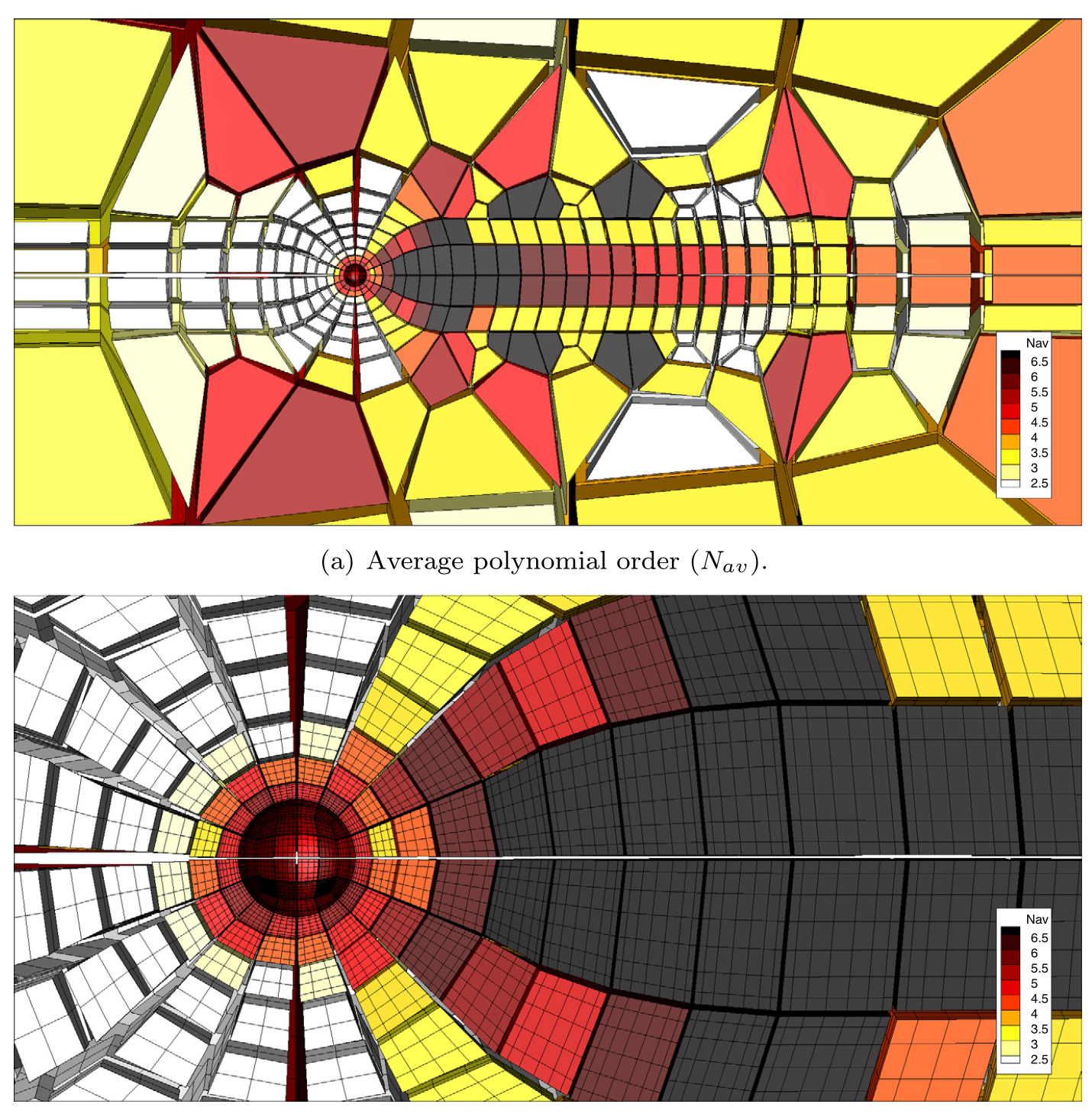
Figure 1: Example of a p-adapted mesh for the flow around a sphere at Reynolds 200. The contours indicate the average polynomial order (Pav=(P1 +P2 +P3)/3). Taken from [6].

The adaptation process requires the user to select a target truncation error threshold for the adapted mesh. This threshold does not have any direct physical or engineering meaning and has been seen as a drawback of the methodology in the past. However, we have recently shown [60] how to link the truncation error threshold with any flow functional (e.g., lift, drag), bypassing this limitation .

The multiphase flow applications (Sec. 4.3) are of unsteady nature, and thus require the use of dynamic adaptation. In this case, it is crucial to have an adequate resolution in the region of the interface between different fluids. The tracking algorithm uses the value of the phase field parameter $\phi$ of the Cahn-Hilliard equation. The interface is defined as the region where $0.1\leq\phi\leq 0.9$. Thus, knowing the location of the interface throughout the simulation, we adapt the elements that contain part of the interface between different phases. This process, shown in Fig. 2, is detailed in [61, 53], as well as the method through which it can be automated.

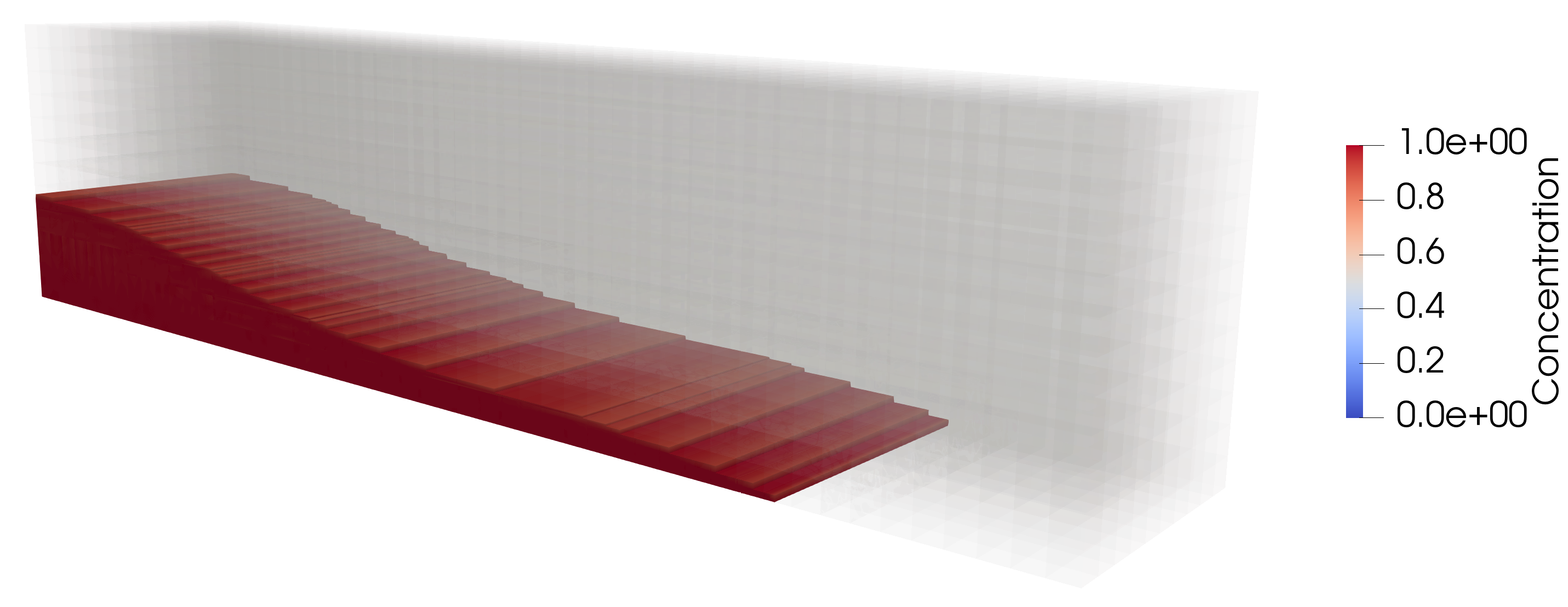
(a) $t=2$

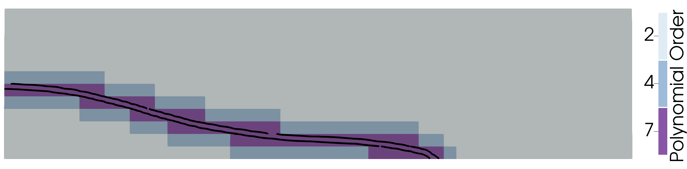
(b) $t=2$

Figure 2: Instances of the dam break test case showing the initial condition and the flow configuration at $t=2\;s$. Taken from [53].

3.7 Time advancement

There are several temporal integration strategies in HORSES3D, which are tailored for specific solvers. By default, the low-storage explicit Runge-Kutta of order 3 [62] is used as a time-stepping strategy for any given problem. This can be changed by the user to an explicit Runge-Kutta 4^th order [63] or to more sophisticated methods described below.

For steady-state simulations, the non-linear p-multigrid method (also known as Full Approximate Scheme – FAS) [6] is employed. FAS employs several explicit (local time-stepping, optimised Runge-Kutta coefficients for steady-state) [64, 65] and semi-implicit (BIRK, LU-SGS, ILU(0)) [66, 67, 68] convergence acceleration strategies, presented in Fig. 4. An example of convergence for a laminar test case is presented in Fig. 3.

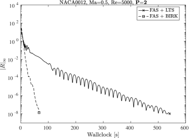
(a)

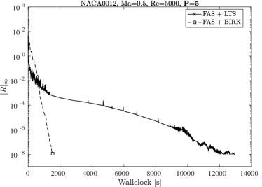
(b)

Figure 3: Figures present convergence for a laminar test case (NACA0012 airfoil with $\text{Re}=5000$, $\text{Ma}=0.5$ and $\text{AoA}=0$) using FAS with explicit and semi-implicit convergence acceleration. The explicit FAS uses a five stage 2${}^{\text{nd}}$ order Runge-Kutta smoother [65] with local time-stepping. The semi-implicit FAS uses the BIRK smoother [68]. A low (left figure) and high (right figure) uniform polynomial discretisations are considered.

For time-accurate simulations (e.g., Large Eddy Simulations), implicit time integration can be used with Backward Difference Formulas (BDF) of order $1,...,5$, or 6^th order Rosenbrock-type Runge-Kutta schemes [69]. The Jacobian can be computed analytically for the Navier-Stokes equations and also numerically when other equations need to be included (e.g., Spalart-Allmaras) using a coloring algorithm [70, 71] to improve performance.

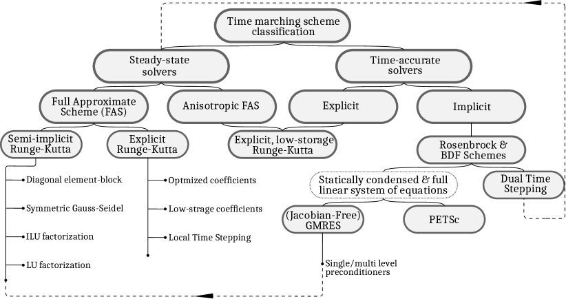
Figure 4: Classification of time-marching schemes employed in HORSES3D.

3.8 Parallelisation and efficiency

To reduce the computational cost, all techniques are parallelised for hybrid systems to run on multiprocessor CPUs combining MPI and OpenMP. Let us note that DG methods have compact stencils for unstructured meshes, and hence are highly parallelisable since each element has many structured internal degrees of freedom (related to the polynomial degree).

Numerical experiments for explicit time-stepping have been performed on the Taylor-Green Vortex (TGV) problem [72]. The TGV problem has been widely used to report the subgrid-scale modelling capabilities of ILES approaches and discretisations [43, 73, 74]. The results are shown in Fig. 5.

We observe very good scalability when using high polynomial orders and MPI + OpenMP architectures up to a thousand cores; see Fig. 5.b, where we get 86% of the ideal performance for 600 cores and $P=6$.

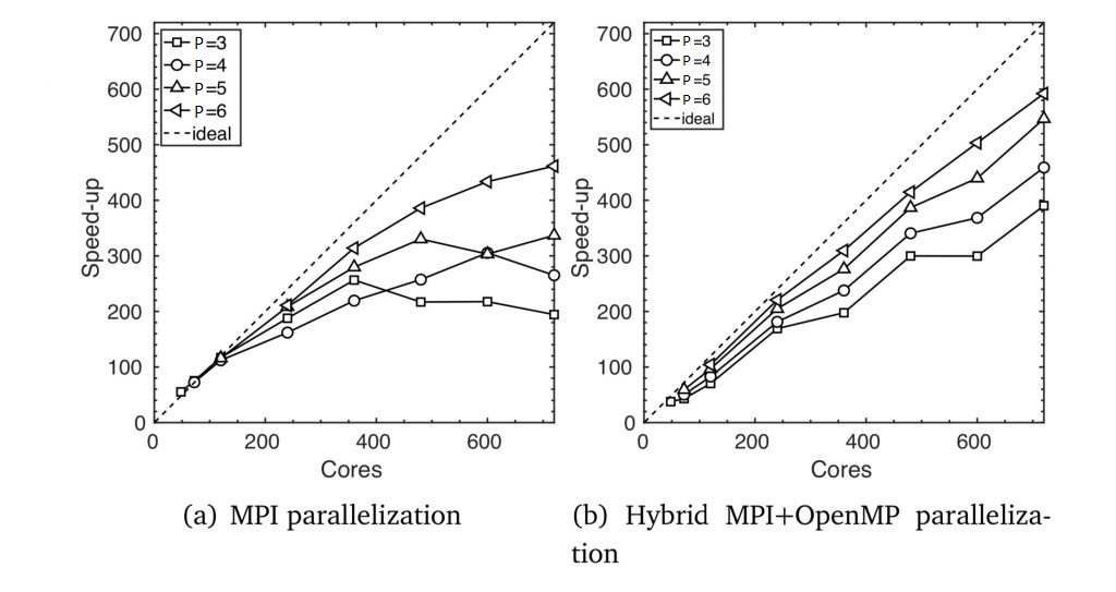
Figure 5: HORSES3D scalability solving the TGV problem with a $64^{3}$ mesh using a) MPI and b) MPI/OpenMP.

4 Multiphysics

In this section, we detail the various multiphysics applications included in HORSES3D. Namely, we detail the turbulence closure models (RANS and LES), the incompressible flow formulation, multiphase modelling, shock capturing, flow-particle dynamics, aeroacoustics and immersed boundaries.

4.1 Turbulence closure models

A particular challenge related to the numerical simulation of fluid flows relates to turbulence modelling. The main characteristic of turbulent flows is the presence of a broad spectrum, where a wide range of length and time scales coexist [75]. It is the multiscale character (in time and space) of turbulent flows, which scales with the Reynolds number (i.e. ratio of inertia to viscous forces) that renders the numerical treatment of turbulence a difficult task.

The Direct Numerical Simulation (DNS) approach solves the Navier-Stokes equations without additional modelling. Consequently, it requires a very high spatial and temporal resolution and is thus restricted to moderately low Reynolds. To compute large Reynolds number flows in complex configurations, it is necessary to introduce a certain degree of modelling to limit the cost. There are two main approaches: the Reynolds Averaged NS (RANS) approach and the Large Eddy Simulation (LES) technique. Both types are included in HORSES3D.

The RANS solver uses the negative Spalart-Allmaras model from [76, 64], while the LES models consider both explicit or implicit subgrid modelling. An example of the results derived using the HORSES3D framework is presented in Figure 6, where we consider the Common Research Model [77].

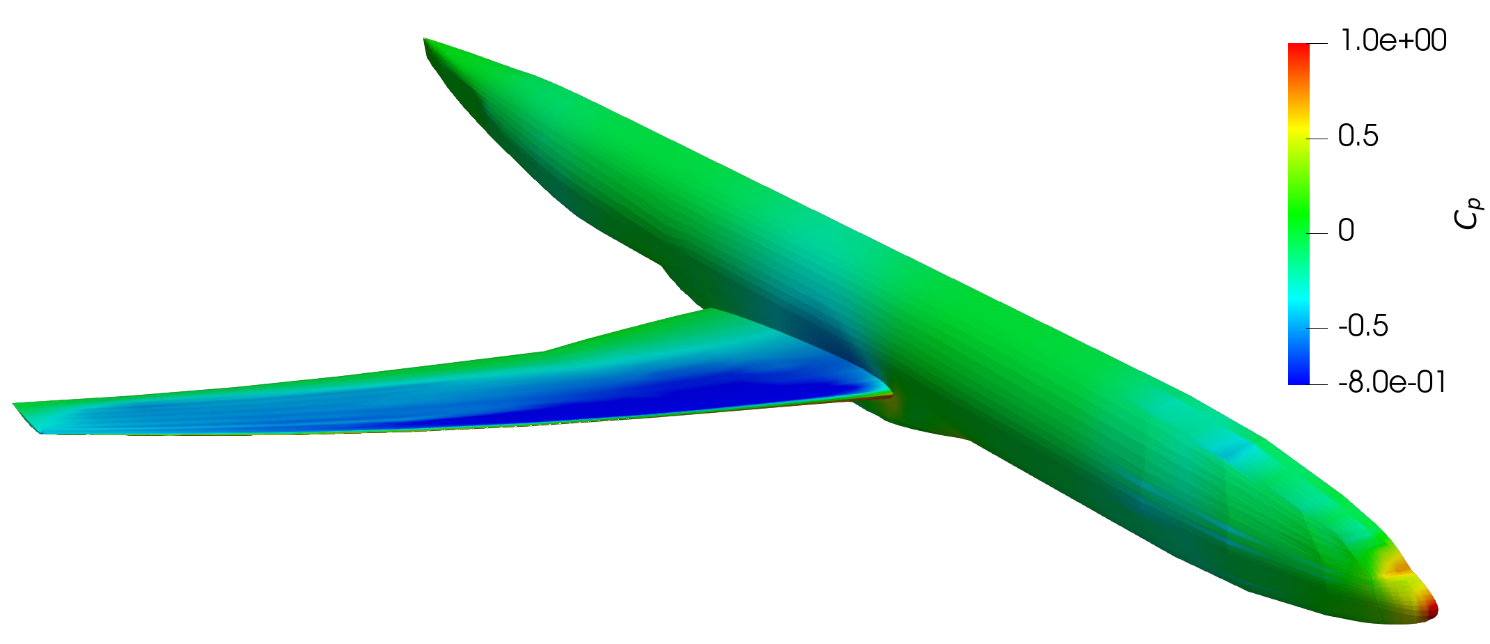
(a)

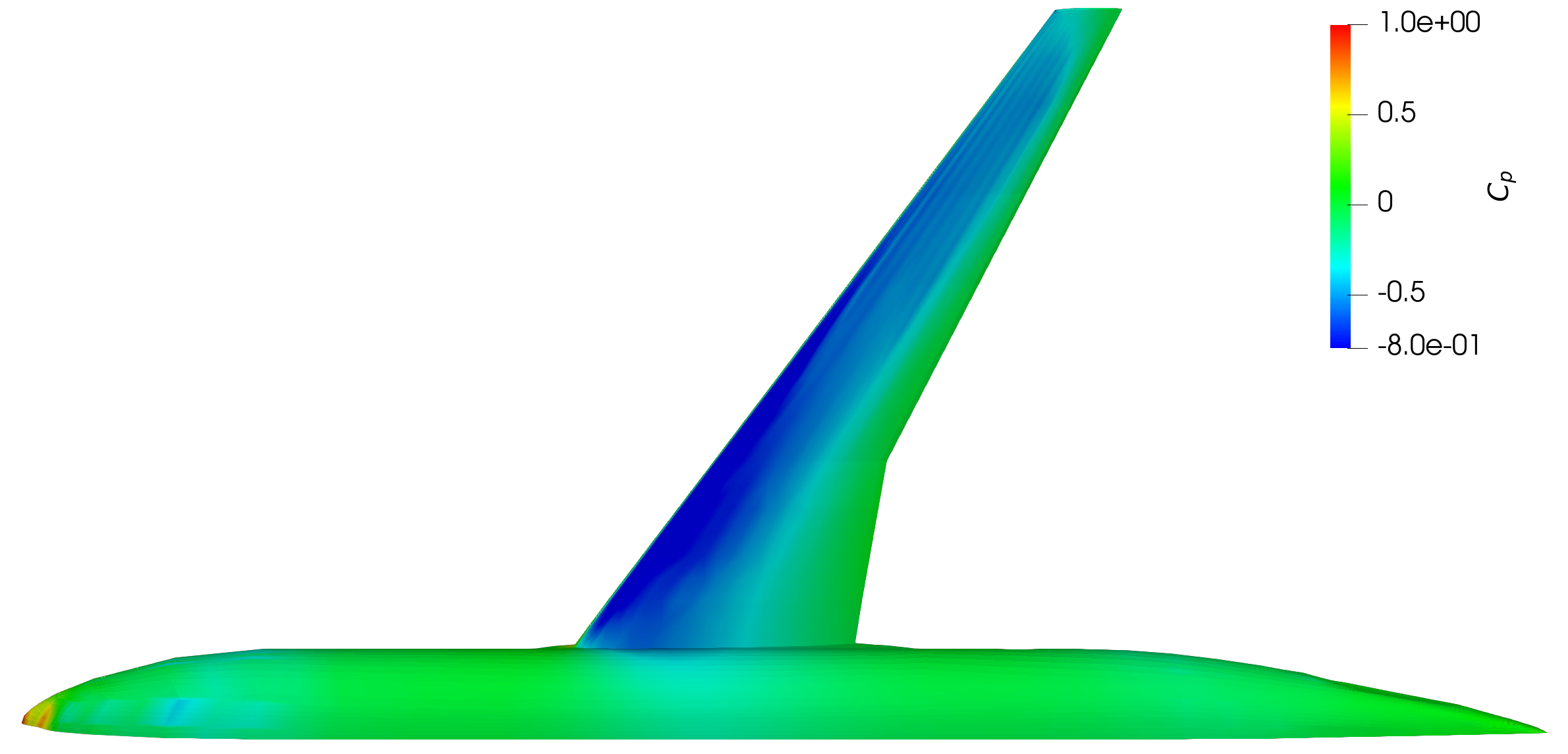
(b)

Figure 6: Pressure contour over the surface of the Common Research Model (CRM) for M=0.85, Re=$5\cdot 10^{6}$ and AoA = $2.3^{\circ}$ using the HORSES3D RANS module with split-form inviscid fluxes. The computations have been done on a $\mathrm{3^{rd}}$ order ($P=2$) hexahedral mesh from [78].

The explicit LES approach uses spatial filtering where the large structures are resolved, reducing the modelling to the small unresolved turbulent structures (i.e. small eddies), which behave in an isotropic fashion. We have implementations for classic LES models, including Smagorinsky [79, 80], Wale [81], and Vreman [82]. In addition, we developed in [74] a SVV-Smagorinsky model where the Spectral Vanishing Viscosity technique was combined with a Smagorinsky LES model to enhance the closure model. The model was capable of maintaining low dissipation levels for laminar flows, while providing the correct dissipation for all wave–number ranges in turbulent regimes.

In recent years, Implicit Large Eddy Simulation (ILES) methods [83] have gained popularity. This approach, increasingly popular when combined with high-order numerical methods (e.g., DG), uses the dissipation inherited from the numerical scheme to mimic turbulent effects of unresolved scales. DG methods have dissipation and dispersive errors, which are confined to high wavenumbers, and therefore introduce numerical dissipation primarily to under-resolved wave-lengths [84]. This property makes them very suitable for ILES, since dissipation only acts at under-resolved scales, as explained in [29, 85, 86, 87]. Riemman solvers are the classic option to include numerical dissipation in DG schemes [1, 35], since they naturally arise when discretising the non-linear terms. A comparison of different fluxes for homogeneous turbulence can be found in [88, 74]. A different option is to modify the viscous terms to enhance the approximation’s dissipative properties. The modification has been proposed in [29] using an increased penalty parameter (compared to the minimum required to ensure coercivity of the scheme) when discretising the viscous terms using an interior penalty formulation.

When combined with high-order DG methods, ILES provide valuable results even for challenging problems such as the prediction of turbulent quantities, detached flows and laminar-turbulent transition on airfoils, see, for example, [89, 29, 90, 83, 74, 91, 92]. Finally, a promising approach is to combine robust energy-stable methods (e.g., skew symmetric variants) with ILES techniques (e.g., Spectral Vanishing Viscosity) to provide accurate simulation at high Reynolds numbers, see [85, 74]. As an example of ILES performance, we calculated the averaged values for the lift and drag on a NACA0012, using a hexahedral mesh with 18000 elements, with $P=4$ (2.2 million degrees of freedom). Fig. 7 compares the aerodynamic coefficients with the experimental data for various angles of attack and the two solvers. Fig. 7 [Left] shows the lift coefficient against AoA and Fig. 7 [Right] depicts the lift-drag polar for $\text{Re}=1\times 10^{6}$. We observe very good agreement with the experimental data.

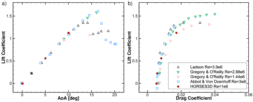
Figure 7: Lift and drag for a NACA 0012 at Re=1e6; comparisons between HORSES3D (ILES version) with experimental data. Adapted from [90]

4.2 Incompressible Flows

Among the various incompressible Navier-Stokes models, HORSES3D uses an artificial compressibility formulation [93], which converts the elliptic problem into a hyperbolic system of equations, at the expense of a non divergence–free velocity field. However, it allows one to avoid constructing an approximation that satisfies the inf–sup condition, see [94, 95] and the references therein. The artificial compressibility model is commonly combined with dual time–stepping, which solves an inner pseudo-time-step loop until velocity divergence errors are lower than a selected threshold and then performs the physical time marching. This methodology is well suited for use as a fluid flow engine for interface–tracking multiphase flow models, as it allows the density to vary spatially $\rho\left(\vec{x},t\right)$. The artificial compressibility system of equations is

$$\rho_{t}+\vec{\nabla}\cdot\left(\rho\vec{u}\right)=0,$$ (9)

$$\left(\rho\vec{u}\right)_{t}+\vec{\nabla}\cdot\left(\rho\vec{u}\vec{u}\right)=-\vec{\nabla}p+\vec{\nabla}\cdot\left(\frac{1}{\mathrm{Re}}\left(\vec{\nabla}\vec{u}+\vec{\nabla}\vec{u}^{T}\right)\right)+\frac{1}{\mathrm{Fr^{2}}}\rho\vec{e}_{g},$$ (10)

$$p_{t}+c_{0}^{2}\vec{\nabla}\cdot\vec{u}=0,$$ (11)

where Re is the Reynolds number, Fr is the Froude number, $c_{0}^{2}$ is the artificial speed of sound, and $\vec{e}_{g}$ is the gravitational acceleration.

4.3 Multiphase

Phase field models describe the phase separation dynamics of two immiscible liquids by minimising a chosen free–energy. For an arbitrary free–energy function, it is possible to construct different phase field models. Among the most popular, one can find the Cahn–Hilliard [96] and the Allen–Cahn [97] models. The popularity of the first, despite being a fourth-order operator in space, comes from its ability to conserve the phases. HORSES3D permits the solution of the Cahn-Hilliard equation. For a detailed explanation of the model, see [98].

The multiphase flow solver implemented in HORSES3D is constructed by a combination of the diffuse interface model of Cahn–Hilliard [96] with the incompressible Navier–Stokes equations with variable density and artificial compressibility [93]. This model is entropy stable and guarantees phase conservation with an accurate representation of surface tension effects. For a detailed explanation of the model, see [28]. The modified entropy-stable version approximates

$$c_{t}+\vec{\nabla}\cdot\left(c\vec{u}\right)=M_{0}\vec{\nabla}^{2}\mu,$$ (12)

$$\sqrt{\rho}\left(\sqrt{\rho}\vec{u}\right)_{t}+\vec{\nabla}\cdot\left(\frac{1}{2}\rho\vec{u}\vec{u}\right)+\frac{1}{2}\rho\vec{u}\cdot\vec{\nabla}\vec{u}+c\vec{\nabla}\mu=-\vec{\nabla}p+\vec{\nabla}\cdot\left(\eta\left(\vec{\nabla}\vec{u}+\vec{\nabla}\vec{u}^{T}\right)\right)+\rho\vec{g},$$ (13)

$$p_{t}+\rho_{0}c_{0}^{2}\vec{\nabla}\cdot\vec{u}=0,$$ (14)

where $c$ is the phase field parameter, $M_{0}$ is the mobility, $\mu$ is the chemical potential, $\eta$ is the viscosity and $c_{0}$ is the artificial speed of sound. In [28], we provide a comparison between standard and entropy-stable discretisations. Through several numerical experiments, the superior robustness characteristics of the entropy-stable scheme are highlighted in comparison to the standard scheme. Among the test cases considered, there is a two–phase flow of oil and water within a pipe [28] and a 3D dam break test case [53].

For phase field modelling, it is important to adequately resolve the region of the interface between different phases, as it contains large gradients. In HORSES3D, the local refinement around the interface is carried out through p-adaptation. The original scheme presented in [28] has been extended to support p-non-conforming elements and has been modified accordingly so that it is entropy-stable even for p-non-conforming elements, see Fig. 8. The detailed analysis and modifications to the original scheme are presented in [53].

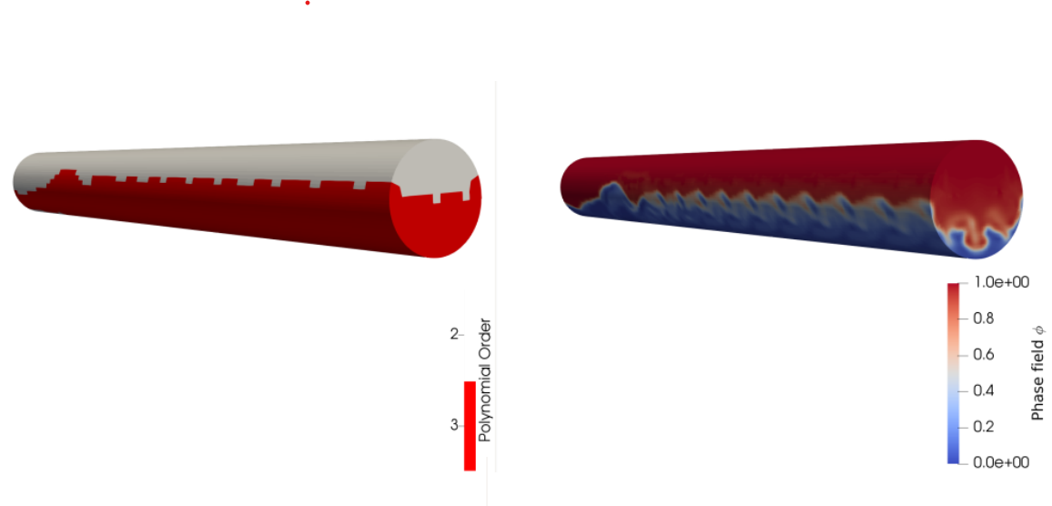
Figure 8: Annular flow test case of water and oil. On the left, the polynomial order distribution is presented for the p-adaptive scheme based on the interface tracking refinement. On the right, the flow structure is presented for the developed flow. Taken from [53].

4.4 Shock capturing

Supersonic flows present additional difficulties to high-order spectral elements, where the favourable accuracy and convergence properties of these schemes can be damaged by the Gibbs phenomenon near shocks. HORSES3D implements a special type of artificial viscosity to handle shocks. In the case of the Navier-Stokes equations, discontinuities due to compressibility effects have an actual width proportional to the viscosity, $\mu$ [99]. This motivates the introduction of an artificial viscous term  $\accentset{\,\leftrightarrow}{\mathbf{F}}_{a}$ into the equations to control the effective $\mu$ at each element to smooth the solution.

HORSES3D includes two options for $\accentset{\,\leftrightarrow}{\mathbf{F}}_{a}$: the viscous flux of the Navier-Stokes equations and the Guermond-Popov entropy-stable flux [100], which also includes a regularisation term in the density equation. Regardless of the selected viscous flux, and to minimise artificial viscosity in smooth regions, we introduce an Spectral Vanishing Viscosity (SVV) formulation and apply a frequency-dependent filter kernel $\mathcal{F}$ to these fluxes, so that the additional term has the form $\accentset{\,\leftrightarrow}{\mathbf{F}}_{a}^{\mathcal{F}}=\mathcal{F}\star\accentset{\,\leftrightarrow}{\mathbf{F}}_{a}$. We implement the filter kernels of [101, 102, 103]. Since the code is a nodal DGSEM framework, we transform the fluxes to the Legendre modal space, $\{L_{i}\}$, where the application of this filter is simply an element-wise product of the fluxes and the kernel, and then we return to the nodal space to recover the filtered flux.

The stability of this new term is analysed in terms of the evolution of the entropy. Physically plausible solutions of the Navier-Stokes equations must agree with elemental laws such as the conservation of the energy or a non-decreasing entropy. We impose this by defining a mathematical entropy function that represents the underlying law and requiring it to be bounded. In this case, the mathematical entropy, $S$, is defined in terms of the non-decreasing physical entropy as

$$S=-\rho s,\quad s=\ln p-\gamma\ln\rho.$$ (15)

We also introduce the concept of entropy variables $\bm{w}$, which are computed from (15) as

$$\bm{w}=\frac{\partial S}{\partial\bm{u}},\quad\bm{u}=(\rho,\rho\vec{v},\rho e)^{T}.$$ (16)

To ensure the stability of the new term, a detailed semi-discrete entropy analysis (see [104, 105, 52]) shows that filtering has to be applied in a very specific form. Expressing the baseline flux as

$$\accentset{\,\leftrightarrow}{\mathbf{F}}_{a}=\mathcal{B}\accentset{\,\leftrightarrow}{\mathbf{G}},\quad\mathcal{B}=\mathcal{L}^{T}\mathcal{D}\mathcal{L},\quad\accentset{\,\leftrightarrow}{\mathbf{G}}=\nabla\bm{w},$$ (17)

where $\mathcal{B}$ is a symmetric matrix, and $\mathcal{L}$ and $\mathcal{D}$ are the matrices of its $\textbf{L}^{T}\textbf{D}\textbf{L}$ decomposition, the filtered flux, $\accentset{\,\leftrightarrow}{\mathbf{F}}_{a}^{\mathcal{F}}$, is obtained by filtering only one half of (17),

$$\accentset{\,\leftrightarrow}{\mathbf{F}}_{a}^{\mathcal{F}}=\frac{1}{\sqrt{J}}\mathcal{L}^{T}\sqrt{\mathcal{D}}\mathcal{F}\star\left(\sqrt{J\mathcal{D}}\mathcal{L}\accentset{\,\leftrightarrow}{\mathbf{G}}\right),$$ (18)

where $J$ is the Jacobian of the transformation from the reference element to the physical elements of the mesh, see Sec. 3.3. A detailed explanation of this derivation can be found in [106].

The SVV approach has proven to be useful for the simulation of turbulent and supersonic flows (see Figure 9); however, the treatment of discontinuities requires a higher amount of dissipation that can be achieved only by adding non-filtered dissipation in troubled regions. Since this is only required near discontinuities, we use a sensor, $s_{\rho}$, based on the average value of the density gradient to detect troubled elements and modify the filter there,

$$s_{\rho}=\int_{el}J\lvert\nabla_{\xi}\rho\rvert^{2}.$$ (19)

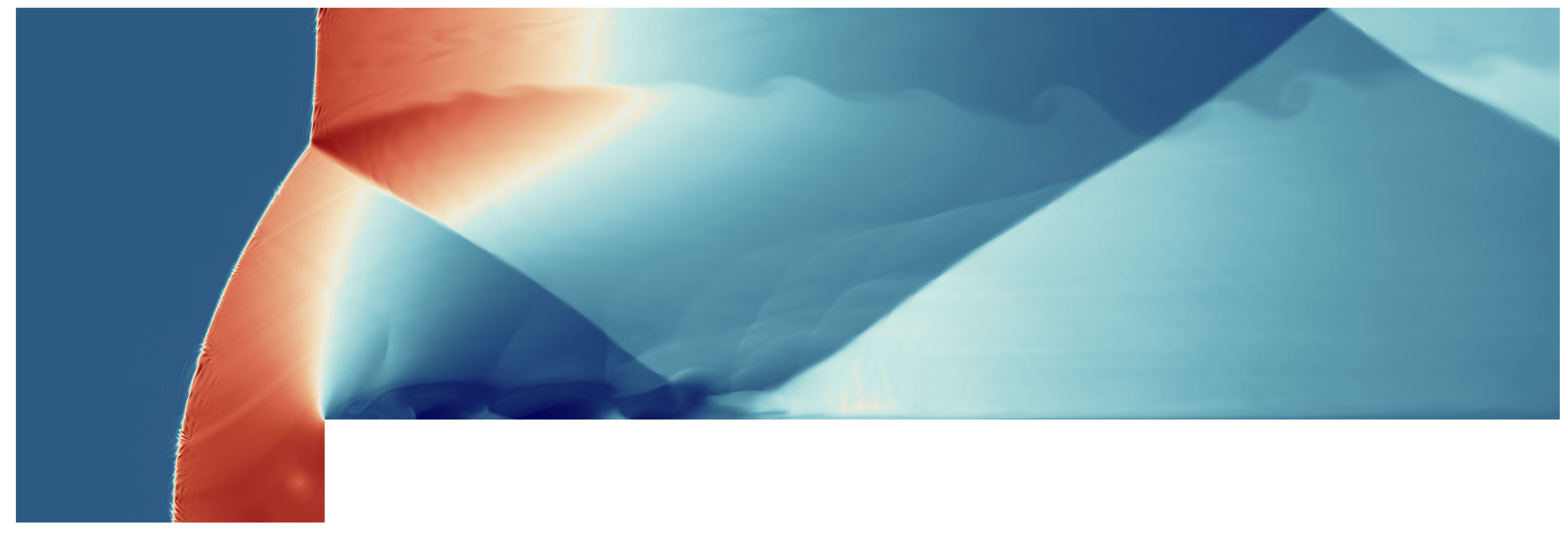
Figure 9: Facing forward step case at $\tau=10$ with an incoming flow at Ma=3 and 3653 elements with polynomial degree $P=7$. Adapted from [106].

4.5 Particles

HORSES3D includes a two-way coupled Lagrangian solver. The model presented here is based on [107].

Particles are tracked along their trajectories, according to the simplified particle equation of motion, where only contributions from Stokes drag and gravity are retained,

$$\frac{dy_{i}}{dt}=u_{i},\quad\frac{du_{i}}{dt}=\frac{v_{i}-u_{i}}{\tau_{p}}+g_{i},$$ (20)

where $u_{i}$ and $y_{i}$ are the ith components of velocity and position of the particle, respectively. Furthermore, $v_{i}$ accounts for the continuous velocity of the fluid at the position of the particle. We consider spherical Stokesian particles, so their mass and aerodynamic response time are $m_{p}=\rho_{p}\pi D_{p}^{3}/6$ and $\tau_{p}=\rho_{p}D_{p}^{2}/18\mu$, respectively, $\rho_{p}$ being the particle density and $D_{p}$ the particle diameter.

Each particle is considered to be subject to a radiative heat flux $I_{o}$. The carrier phase is transparent to radiation, whereas the incident radiative flux on each particle is completely absorbed. Because we focus on relatively small volume fractions, the fluid-particle medium is considered to be optically thin. Under these hypotheses, the direction of the radiation is inconsequential, and each particle receives the same radiative heat flux, and its temperature $T_{p}$ is governed by

$$\frac{d}{dt}(m_{p}c_{V,p}T_{p})=\frac{\pi D_{p}^{2}}{4}I_{o}-\pi D_{p}^{2}h(T_{p}-T),$$ (21)

where $c_{V,p}$ is the specific heat of the particle, which is assumed to be constant with respect to temperature. $T_{p}$ is the particle temperature and $h$ is the convective heat transfer coefficient, which for a Stokesian particle can be calculated from the Nusselt number $Nu=hD_{p}/k=2$.

In practical simulations, integrating the trajectory of every particle is too expensive. Therefore, particles are agglomerated into parcels, each of them accounting for many particles with the same physical properties, position, velocity, and temperature. The evolution of the parcels is tracked with the same set of equations presented for the particles.

The two-way coupling means that fluid flow is modified because of the presence of particles. Therefore, the Navier-Stokes equations (1) are enriched with the following source terms:

$$\bm{S}=\beta\left[\begin{array}[]{c}0\\ \sum_{n=1}^{N_{p}}\frac{m_{p}}{\tau_{p}}(u_{1,n}-v_{1})\delta(\mathbf{x}-\mathbf{y}_{n})\\ \sum_{n=1}^{N_{p}}\frac{m_{p}}{\tau_{p}}(u_{2,n}-v_{2})\delta(\mathbf{x}-\mathbf{y}_{n})\\ \sum_{n=1}^{N_{p}}\frac{m_{p}}{\tau_{p}}(u_{3,n}-v_{3})\delta(\mathbf{x}-\mathbf{y}_{n})\\ \sum_{n=1}^{N_{p}}\pi D_{p}^{2}h(T_{p,n}-T)\delta(\mathbf{x}-\mathbf{y}_{n})\end{array}\right],$$ (22)

where $\delta$ is the Dirac delta function, $N_{p}$ is the number of parcels, $\beta$ is the number of particles per parcel and $u_{i,n}$, $\mathbf{y}_{i,n}$, $T_{p,n}$ are the velocity, spatial coordinates, and temperature of the parcel nth.

The ordinary differential equation (ODE) system (20), (21) that controls the evolution of parcels is integrated in time using a low storage Runge-Kutta 3 method [62]. Integration is separated from the integration of the Navier-Stokes equations. The properties of the fluid (velocity, viscosity, and temperature) at the position of the parcel are evaluated using the interpolation routines included in HORSES3D. These routines work at the element level, so a routine to find the element to which the parcel belongs in general unstructured meshes is also included. The Dirac delta, $\delta(\mathbf{x}-\mathbf{y}_{n})$, which appears in the source term, see (22), can be dealt with in a simple way in the DG setting, since it can be integrated exactly in the weak form.

The coupled-particle model has been used to analyse a particle-laden flow in a channel subject to radiation, which is representative of particle solar radiation systems. Details of the test case can be found in [108]. The results obtained with HORSES3D were obtained with a Cartesian mesh of 4000 elements and a number of particles per parcel $\beta=160$, see Fig. 10. The results of HORSES3D are compared in Fig. 11 with the one-dimensional and three-dimensional simulations performed in [108]. The results of HORSES3D do not exactly match the three-dimensional simulations of [108] as the effect of preferential concentration at the inlet was not considered. Besides HORSES3D uses parcels (agglomerations of particles). This artificial concentration of particles creates local peaks in temperature, which results in an increase of the average temperature.

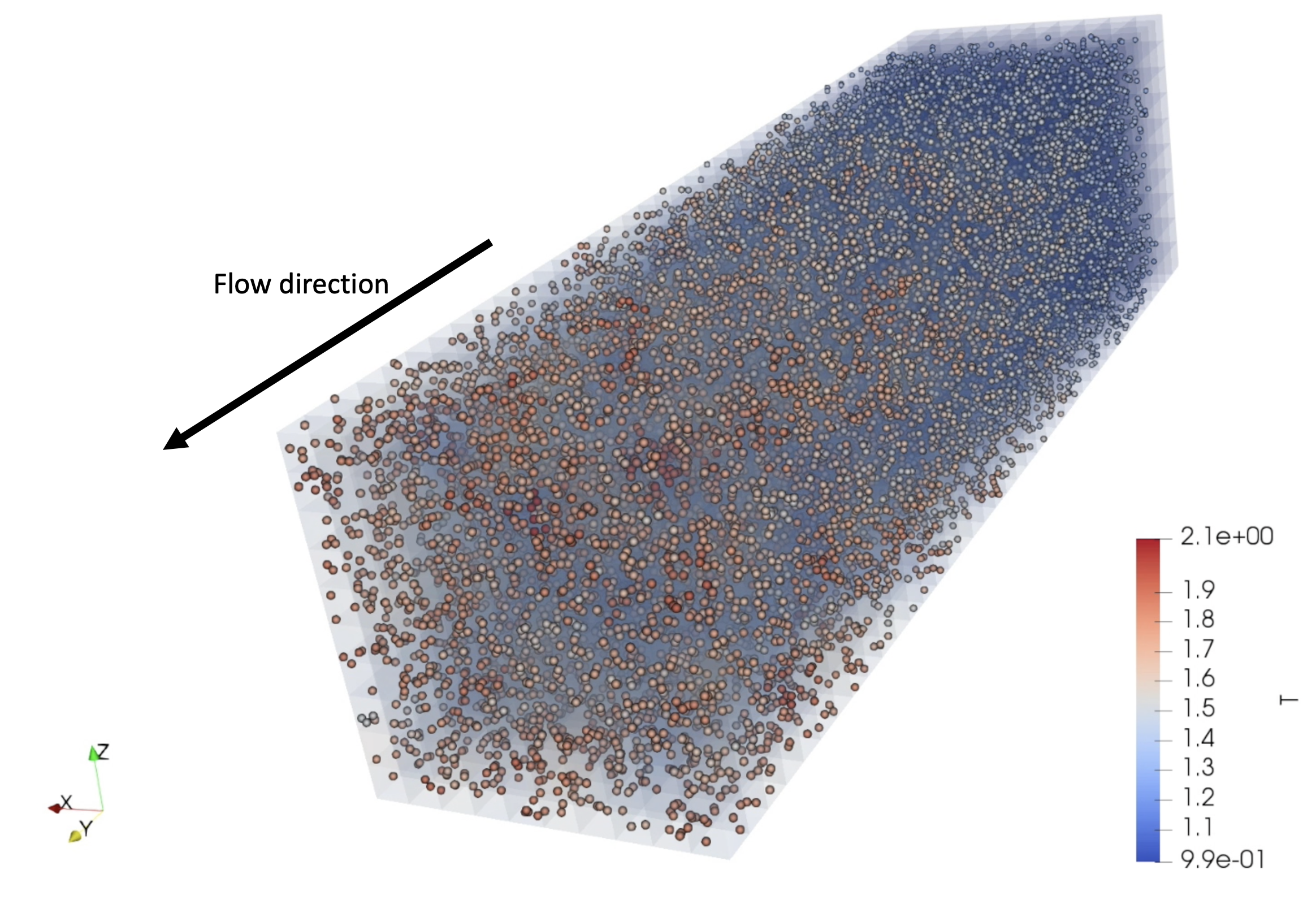
Figure 10: Visualisation of a particle-laden flow in a channel subject to radiation. Particles and gas are injected into the channel at the same temperature. The temperatures of the particles increase in the direction of the flow as a result of the effect of radiation. Details of the test case are given in [108].

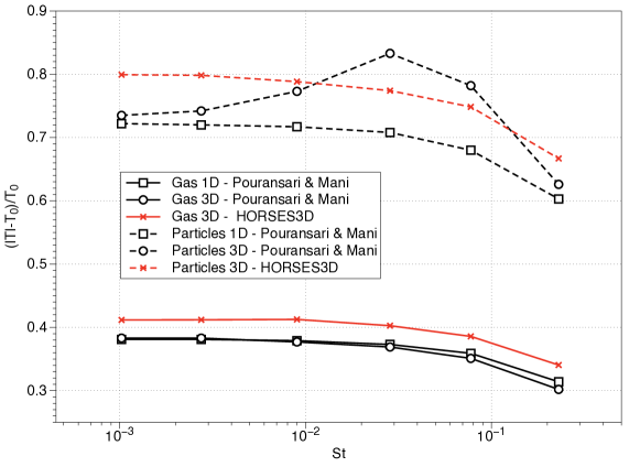
Figure 11: Mean temperatures of gas and particles at the outlet of a channel subject to radiation. $T_{0}=300$ K is the reference temperature, while $St$ is the Stokes number. Details of the test case are given in [108].

4.6 Computational Aeroacoustics

Computational aeroacoustics (CAA) can be divided into two categories. The first one, noise generation, is characterised by turbulence and non-linear interactions near solid surfaces. The second category is noise propagation and can be simplified to a linear propagation of the sound waves.

An approach in CAA is to solve the near and far fields together, using the compressible Navier–Stokes equations on the whole domain, obtaining all the physical effects on the solution without needing external models. This approach is called Direct Noise Computation (DNC), and can deal with complex acoustics, such as acoustic feedback. The compressible Navier–Stokes of HORSES3D is spectrally accurate and therefore well suited to provide accurate acoustics (e.g., pressure fluctuations).

The other possibility for CAA is to use acoustic analogies, which decouple the near and far fields into two computational regions, the so-called hybrid approach. Here, the CAA solution becomes a two-step process, where the near field is computed first and independently of the propagation [109] using the HORSES3D compressible Navier–Stokes solver. Subsequently, equivalent acoustic sources can be extracted from the well-resolved near-field region, to feed the propagation problem, which is solved in the far field. This decoupling enables faster computations since the near-field that requires highly accurate flow computations can be performed separately from the acoustic propagation step.

HORSES3D can compute aeroacustics using the direct approach and also acoustic analogies. In particular, the Ffowcs-Williams and Hawkings (FWH) aeroacoustic analogy [110] is implemented. FWH rearranges the compressible NS equations into an inhomogeneous wave equation. The solution of this wave equation can be obtained in an integral representation (computed numerically). The FWH uses a fictitious surface located in the near-field, where the Navier–Stokes solution is gathered and used to calculate the integral solution. This surface can coincide with the solid boundary of the body (having a solid surface) or be located at an arbitrary position in the flow field (being a permeable surface). HORSES3D allows both possibilities.

Our implementation follows the formulation by Najafi [111], and Ghorbanias [112], where the equations are recast as a convective wave equation. This formulation clearly separates the flow velocity fluctuations ($v_{i}$), surface velocities ($v_{i}$), and the free-stream velocity ($U_{0i}$) as follows:

$$\begin{split}&\bigg{(}\frac{\partial^{2}}{\partial t^{2}}+U_{0i}U_{0j}\frac{\partial^{2}}{\partial x_{i}\partial x_{j}}+2U_{0i}\frac{\partial^{2}}{\partial x_{i}\partial t}-c_{0}^{2}\frac{\partial^{2}}{\partial x_{i}\partial x_{i}}\bigg{)}(H(f)\rho^{\prime})=\\ &\bigg{(}\frac{\partial}{\partial t}+U_{0i}\frac{\partial}{\partial x_{i}}\bigg{)}\big{(}Q_{i}n_{i}\delta(f)\big{)}-\frac{\partial}{\partial x_{i}}\big{(}L_{ij}n_{j}\delta(f)\big{)}+\frac{\partial^{2}}{\partial x_{i}\partial x_{j}}\big{(}T_{ij}H(f)\big{)},\end{split}$$ (23)

where the zero subscript refers to the undisturbed or free-stream flow, $\rho^{\prime}$ is the density fluctuation, $Q_{i}$, $L_{ij}$, $T_{ij}$ are the loading, thickness, and quadrupole terms, respectively, $n_{i}$ is the $i^{th}$ component of the normal at the surface, $H(f)$ is the Heaviside function and $\delta(f)$ is the Dirac delta function. The right-hand side of (23) represents the source terms for the FWH noise model and are calculated from the velocities and pressure (and its time derivative) that are computed by the compressible Navier-Stokes solver. In this implementation, quadrupoles are neglected and so are their contributions to the viscous stress tensor, but they can be easily added if necessary.

The acoustic pressure $p^{\prime}=p-p_{0}$ can be obtained from the density fluctuation, as $p^{\prime}=c_{0}^{2}\rho^{\prime}$ in the far field (where $\rho^{\prime}/\rho_{0}<<1$). For wind tunnel scenarios, most of the terms needed to solve (23) cancel out, and as a result, only two components of the acoustic pressure fluctuation are solved, namely

$$p^{\prime}(\mathbf{x},t)=p_{T}^{\prime}(\mathbf{x},t)+p_{L}^{\prime}(\mathbf{x},t),$$ (24)

$$4\pi p_{T}^{\prime}=\int_{S}{\Bigg{[}\frac{\big{(}1-M_{0i}R_{i}\big{)}\dot{Q_{i}}n_{i}}{R^{*}}\Bigg{]}_{\tau_{e}}dS}\\ -\int_{S}{\Bigg{[}\frac{U_{0i}\hat{R^{*}_{i}}Q_{i}n_{i}}{R^{*2}}\Bigg{]}_{\tau_{e}}dS},$$ (25)

$$4\pi p_{L}^{\prime}=\int_{S}{\Bigg{[}\frac{\dot{L}_{ij}n_{j}\hat{R_{i}}}{c_{0}R^{*}}\Bigg{]}_{\tau_{e}}dS}\\ +\int_{S}{\Bigg{[}\frac{L_{ij}n_{j}\hat{R^{*}_{i}}}{R^{*2}}\Bigg{]}_{\tau_{e}}dS},$$ (26)

where $p_{T}$ is the thickness pressure fluctuation, $p_{L}$ is the loading pressure fluctuation, $c_{0}$ is the speed of sound, $M_{0}$ is the free-stream Mach number, $U_{0}$ is the free-stream velocity, $R$ is the phase radius, $R^{*}$ the amplitude radius (see [113] for a more detailed explanation), and the hat ( $\hat{}$ ) of both $R$ and $R^{*}$ represents the partial derivatives of the radius quantities. The subscript $\tau_{e}$ indicates that the integrals are calculated at the emission retarded time defined as $\tau_{e}=t-R/c_{0}$, see [114] for more details.

For static observers, the retarded time can be calculated analytically, as opposed to when considering bodies with motion. A source time-dominant algorithm is used [115], where at each numerical time-step (also known as emission time) the observer time is calculated, allowing for a time-advancing approach. All integrals from (25) and (26) are numerically evaluated on each h-mesh face of the FWH surface, using the high-order (p-mesh) discretisation at the face, which is inherently related to the Gauss-Legendre (or Gauss-Lobatto) nodes.

A classic validation case for evaluating an FWH implementation is the stationary monopole in a moving medium [116]. The tested monopole has a reference length $l=1$, an amplitude $A/(lc_{0})=9.98\times 10^{-5}$, an angular frequency $\omega l/c_{0}=4\pi$, a free-stream Mach number $M_{0}=0.5$, and a centre at the origin $x_{0}=[0,0,0]$. Fig. 12 shows the prediction of the acoustic pressure for an observer located at $500l$ in the streamwise direction, where a good prediction of the frequency against the analytical solution is obtained, while there is a relative error of around 7% for the amplitude.

Another case of classical study is the sound generated by an airfoil in an external flow [117, 118], where the noise is scattered by the trailing edge. The setup is a NACA 0012 at $\text{Re}=1\times 10^{5}$ based on the airfoil chord, and $\text{Ma}=0.4$. DNC computations can be performed in the near field, as shown in Fig. 13(a) for the dilation field, where acoustic waves can be seen to be generated at the trailing edge and propagated to the far field. Furthermore, the directivity of the acoustic pressure in the far field (at a $r=2C$) can be seen in Fig. 13(b), computed by the FWH analogy. The expected dipole shape is obtained for this case.

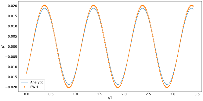
Figure 12: Stationary monopole in a moving medium [116]. Comparison between analytical and FWH acoustic pressure.

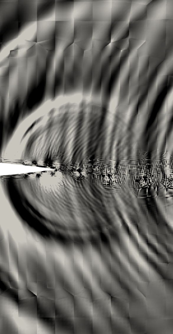
(a)

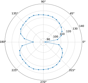
(b)

Figure 13: NACA 0012 aeroacoustics at $\text{Re}=1\times 10^{5}$.

4.7 Mesh free - Immersed Boundary method

In addition to classic body fitted simulations, HORSES3D includes an Immersed Boundary (IB) technique. IB is a mesh-free method that allows the simulation of complex and moving geometries on simple Cartesian meshes. By avoiding the necessity of body fitting mesh, the grid generation process can be skipped, thus shortening a very time-consuming step.

IB was first introduced by Peskin [119] and comes in many flavours; see the review by Kim and Choi [120]. A possible implementation of IB is volume penalisation, where to simulate the presence of a geometry, a source term is applied to the Navier-Stokes equations. This approach has recently been extended to high-order methods by our group [121, 122]. The method is simple, robust, and can be easily extended to moving geometries.

The IB mask $\chi(\vec{x},t)$ distinguishes the penalised region (inside the geometry) $\Omega_{s}$ and the outer region (fluid region), $\Omega_{f}$, as

$$\chi(\vec{x},t)=\begin{cases}1,&\text{if }\vec{x}\in\Omega_{s}\\ 0,&\text{if }\vec{x}\in\Omega_{f},\end{cases}$$ (27)

where $\vec{x}$ is the coordinate vector. The geometry is considered to be a porous media whose permeability approaches zero to mimic solid geometries. Given the velocity of the geometry $\vec{u}_{s}=\left(u_{s},v_{s},w_{s}\right)$, a source term

$$\textbf{S}=\frac{\chi}{\eta}\begin{pmatrix}0\\ \rho u_{s}-\rho u\\ \rho v_{s}-\rho v\\ \rho w_{s}-\rho w\\ \frac{\rho}{2}\left(u_{s}^{2}+v_{s}^{2}+w_{s}^{2}\right)-\frac{\rho}{2}\left(u^{2}+v^{2}+w^{2}\right).\\ \end{pmatrix}$$ (28)

is added to the Navier-Stokes equations, where $\eta$ is the permeability, $\rho$ and $u,v,w$ the density and velocity components, respectively. Once the mask is generated, the source term (28) is applied to the degrees of freedom and the equations are solved.

In HORSES3D, the mask is constructed using a ray-tracing approach. The input is a CAD (STL) file representing the geometry to be simulated and a generic mesh. A surface-area heuristic KD-tree is built that contains the whole body. This type of KD-tree is known to improve the efficiency of the ray-tracing algorithm. The construction of the KD-tree is parallelised using MPI and OpenMP. The OpenMP construction implements breadth-first and depth-first parallelisation. The first is used at the starting levels of the KD-tree where the number of triangles, defining the surface geometry in the STL file, is usually big enough to justify the parallelisation of the loops performed on the objects; the latter is used so that each of the remaining KD-tree’s branches is performed by a single thread (interested readers are referred to [123]). When MPI is used, the CAD file is split into a number of partitions equal to the number of slaves. A KD-tree is built for each partition, reducing the computational time since the total number of triangles in the partitions is smaller than the initial one.

A key aspect of IB is the computation of the aerodynamic forces acting on the body, which requires a reconstruction of the surface data. The idea is to find the value of the state variables on the interpolation points over the body surface (IP) and perform surface integration. In general, for what concerns the IB approach, none of the degrees of freedom where the solution is computed lies on the body surface; hence, interpolation is needed. We use the inverse distance weight to compute the state at each interpolation point:

$$Q_{IP}=\frac{\sum_{i}\frac{Q_{i}}{d_{i}}}{\sum_{i}\frac{1}{d_{i}}},$$ (29)

where $Q_{IP}$ is the state at the interpolation point, $d_{i}$ is the distance between the $i^{th}$-degree of freedom and the surface normal passing through the interpolation point, and $Q_{i}$ is the state at the $i^{th}$-degree of freedom. Data reconstruction is performed starting from the so-called band region, i.e. the set of all degrees of freedom lying in the fluid region ($\Omega_{f}$) close enough to the body surface. These degrees of freedom are candidates for being inside the set of points used for the interpolation. HORSES3D uses a nearest neighbour algorithm to find the $n$ points (where $n$ is a user-defined parameter) closer to the IP point and, once all the values of the IPs are known, integration is performed.

Fig. 14 shows how the IB method can be used to simulate a horizontal wind turbine. In this case the tower and nacelle are static, but the blades rotate with a constant rotational speed. It can be seen that the IB method captures the leading edge accelerations and blade tip vortices without the necessity of generating a complex body-fitted mesh. As an alternative for compute horizontal axis turbines, we have recently implemented various actuator line formulations.

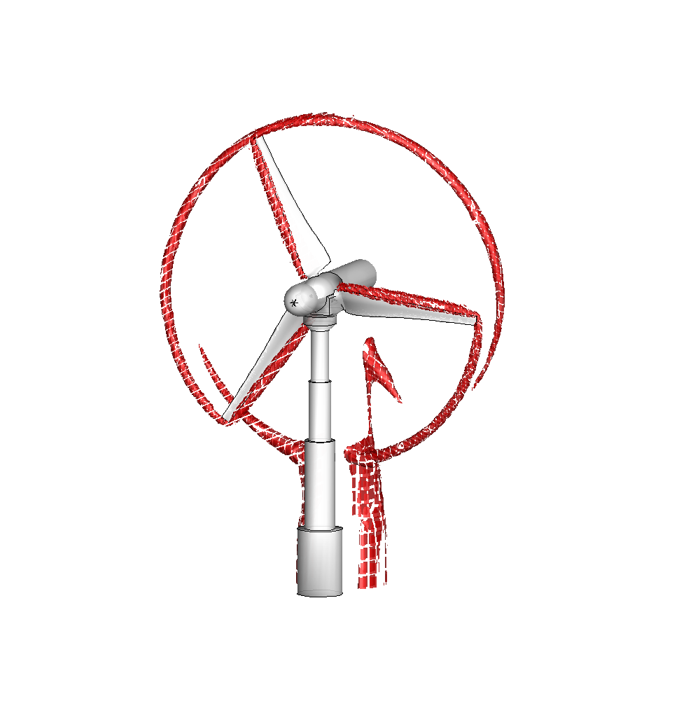
(a)

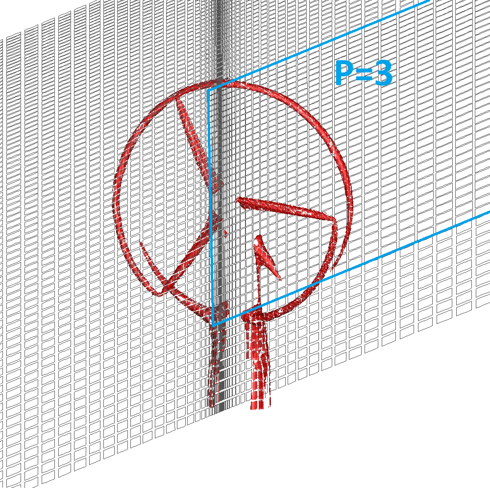
(b)

Figure 14: Wind turbine simulation with immersed boundary method. Isosurface of velocity magnitude showing tip vortex and the acceleration region at the blade leading edge.

5 Licensing, code structure, manuals and test cases

The code is maintained and available on GitHub. HORSES3D is a copyright of NUMATH https://numath.dmae.upm.es under the MIT License. NUMATH (Numerical Methods in Aerospace Technology) is a research group belonging to the School of Aeronautics in Madrid (Universidad Politécnica de Madrid). The objective of the group is to develop high-order numerical methods.

5.1 GitHub and continuous integration

The source code of HORSES3D is stored on GitHub. It has a number of test cases to check the various physics and numerical methods. The objective of test cases is to quickly check if a new commit “breaks” the code. To that end, once a new functionality is implemented, a test case is generated that checks it. The solution of this test case is stored and compared to that obtained with new versions of the code. The process of running the test cases and checking the solutions is integrated within the GitHub workflow framework. It is set to run automatically with a pull request trigger. Furthermore, a more complete test case suit is run on a monthly basis to check the code in more detail (e.g., compilation and run with different compilers in serial/parallel, etc.).

5.2 Documentation

HORSES3D includes a $doc$ folder with documentation and user manuals where all parameters are identified. The solver uses control files, $*.control$, where the parameters and boundary conditions for the simulations are set.

These cases are integrated into the Github workflow framework and run automatically (see previous section).

6 Future directions

We are constantly updating HORSES3D with new features, multiphysics and coupling it with new techniques. For example, we have recently linked HORSES3D to neural networks to accelerate simulations and have allowed the solver to call other external libraries through Python interfaces. Future directions include:

• Neural networks to accelerate high-order methods:

  High-order discontinuous Galerkin methods allow accurate solutions through the use of high-order polynomials inside each mesh element. Increasing the polynomial order leads to high accuracy, but increases the cost. On the one hand, high-order polynomials require more restrictive time-steps when using explicit temporal schemes, and on the other hand, the quadrature rules lead to more costly evaluations per iteration. In a recent work, we propose to accelerate high-order DG methods using Neural Networks. To this aim, we train a Neural Network using a high-order discretisation, to extract a corrective forcing that can be applied to a low order solution with the aim of recovering high-order accuracy. With this corrective forcing term, we can run a low-order solution (low cost) and correct the solution to obtain high-order accuracy; see details in [124, 125].

• Coupling with other solvers (e.g., MFEM [126, 127]) using Python:

  It is often advantageous to link flow solvers with external libraries (e.g., when performing fluid-structure interaction coupling or conjugate heat transfer). In these cases, external libraries can be called to perform part of the simulation (structural calculation or solving heat/radiation). To allow for this flexibility, we have developed an interface from Fortran to Python. Using this interface, it is possible to call Python routines at any point of the CFD calculation. Additionally, it is possible to call other libraries written in C/C++ from Python.

7 Conclusions

HORSES3D is an open-source parallel framework for the solution of non-linear partial differential equations. The solver allows the simulation of compressible flows (with and without shocks), incompressible flows, RANS and LES turbulence models, particle dynamics, multiphase flows, and aeroacoustics. The numerical schemes provide fast computations, especially when selecting high-order polynomials and MPI/OpenMP combinations for a large number of processors. Entropy-stable schemes, local anisotropic p-adaptation, and efficient dual time-stepping and multigrid allow the solver to tackle problems of industrial relevance, such as aircrafts and wind turbines.

The modularity and object-oriented programming architecture allow for easy integration of new physics and numerical methodologies, ensuring the necessary flexibility in a research focused solver.

References

- [1] Z. Wang, R. Fidkowski, K.and Abgrall, F. Bassi, D. Caraeni, A. Cary, H. Deconinck, R. Hartmann, K. Hillewaert, H. Huynh, N. Kroll, G. May, P. Persson, B. van Leer, M. Visbal, High-order CFD methods: current status and perspective, International Journal for Numerical Methods in Fluids 72 (8) (2013) 811–845.
- [2] Z. Wang, A perspective on high-order methods in computational fluid dynamics, Science China Physics, Mechanics & Astronomy 59 (1) (2016) 1–6.
- [3] M. Kompenhans, G. Rubio, E. Ferrer, E. Valero, Adaptation strategies for high order discontinuous Galerkin methods based on Tau-estimation, Journal of Computational Physics 306 (2016) 216–236.
- [4] M. Kompenhans, G. Rubio, E. Ferrer, E. Valero, Comparisons of p-adaptation strategies based on truncation-and discretisation-errors for high order discontinuous Galerkin methods, Computers Fluids 139 (2016) 36–46.
- [5] A. M. Rueda-Ramírez, G. Rubio, E. Ferrer, E. Valero, Truncation error estimation in the p-anisotropic discontinuous Galerkin spectral element method, Journal of Scientific Computing 78 (1) (2019) 433–466.
- [6] A. M. Rueda-Ramírez, J. Manzanero, E. Ferrer, G. Rubio, E. Valero, A p-multigrid strategy with anisotropic p-adaptation based on truncation errors for high-order discontinuous Galerkin methods, Journal of Computational Physics 378 (2019) 209–233.
- [7] D. Gottlieb, S. A. Orszag, Numerical analysis of spectral methods: theory and applications, SIAM, 1977.
- [8] W. H. Reed, T. R. Hill, Triangular mesh methods for the neutron transport equation, Tech. rep., Los Alamos Scientific Lab., N. Mex.(USA) (1973).
- [9] F. Bassi, S. Rebay, A high-order accurate discontinuous finite element method for the numerical solution of the compressible Navier–Stokes equations, Journal of Computational Physics 131 (2) (1997) 267–279.
- [10] F. Bassi, S. Rebay, G. Mariotti, S. Pedinotti, M. Savini, A high-order accurate discontinuous finite element method for inviscid and viscous turbomachinery flows, in: Proceedings of the 2nd European Conference on Turbomachinery Fluid Dynamics and Thermodynamics, Antwerpen, Belgium, 1997, pp. 99–109.
- [11] P. Fischer, J. Kruse, J. Mullen, H. Tufo, J. Lottes, S. Kerkemeier, NEK5000–open source spectral element CFD solver, Argonne National Laboratory, Argonne National Laboratory, Mathematics and Computer Science Division, Argonne, IL (2008).
-
[12]
C. Cantwell, D. Moxey, A. Comerford, A. Bolis, G. Rocco, G. Mengaldo, D. De
Grazia, S. Yakovlev, J.-E. Lombard, D. Ekelschot, B. Jordi, H. Xu,
Y. Mohamied, C. Eskilsson, B. Nelson, P. Vos, C. Biotto, R. Kirby,
S. Sherwin,
Nektar++:
An open-source spectral/hp element framework, Computer Physics
Communications 192 (2015) 205–219.
doi:https://doi.org/10.1016/j.cpc.2015.02.008.
URL https://www.sciencedirect.com/science/article/pii/S0010465515000533 -
[13]
D. Moxey, C. D. Cantwell, Y. Bao, A. Cassinelli, G. Castiglioni, S. Chun,
E. Juda, E. Kazemi, K. Lackhove, J. Marcon, G. Mengaldo, D. Serson,
M. Turner, H. Xu, J. Peiró, R. M. Kirby, S. J. Sherwin,
Nektar++:
Enhancing the capability and application of high-fidelity spectral/hp element
methods, Computer Physics Communications 249 (2020) 107110.
doi:https://doi.org/10.1016/j.cpc.2019.107110.
URL https://www.sciencedirect.com/science/article/pii/S0010465519304175 -
[14]
H. Blackburn, D. Lee, T. Albrecht, J. Singh,
Semtex:
A spectral element–fourier solver for the incompressible
Navier–Stokes equations in cylindrical or Cartesian coordinates,
Computer Physics Communications 245 (2019) 106804.
doi:https://doi.org/10.1016/j.cpc.2019.05.015.
URL https://www.sciencedirect.com/science/article/pii/S0010465519301730 -
[15]
W. Bangerth, R. Hartmann, G. Kanschat,
Deal.II—a general-purpose
object-oriented finite element library, ACM Trans. Math. Softw. 33 (4)
(2007) 24–es.
doi:10.1145/1268776.1268779.
URL https://doi.org/10.1145/1268776.1268779 -
[16]
G. J. Gassner, A. R. Winters, D. A. Kopriva,
Split
form nodal discontinuous Galerkin schemes with summation-by-parts property
for the compressible Euler equations, Journal of Computational Physics 327
(2016) 39–66.
doi:https://doi.org/10.1016/j.jcp.2016.09.013.
URL https://www.sciencedirect.com/science/article/pii/S0021999116304259 -
[17]
F. Hindenlang, G. J. Gassner, C. Altmann, A. Beck, M. Staudenmaier, C.-D. Munz,
Explicit
discontinuous Galerkin methods for unsteady problems, Computers & Fluids
61 (2012) 86–93, ”High Fidelity Flow Simulations” Onera Scientific Day.
doi:https://doi.org/10.1016/j.compfluid.2012.03.006.
URL https://www.sciencedirect.com/science/article/pii/S004579301200093X - [18] H. Ranocha, M. Schlottke-Lakemper, A. R. Winters, E. Faulhaber, J. Chan, G. Gassner, Adaptive numerical simulations with Trixi.jl: A case study of Julia for scientific computing, Proceedings of the JuliaCon Conferences 1 (1) (2022) 77. arXiv:2108.06476, doi:10.21105/jcon.00077.
- [19] M. Schlottke-Lakemper, A. R. Winters, H. Ranocha, G. J. Gassner, A purely hyperbolic discontinuous Galerkin approach for self-gravitating gas dynamics, Journal of Computational Physics 442 (2021) 110467. arXiv:2008.10593, doi:10.1016/j.jcp.2021.110467.
-
[20]
F. Witherden, A. Farrington, P. Vincent,
PyFR:
An open source framework for solving advection–diffusion type problems on
streaming architectures using the flux reconstruction approach, Computer
Physics Communications 185 (11) (2014) 3028–3040.
doi:https://doi.org/10.1016/j.cpc.2014.07.011.
URL https://www.sciencedirect.com/science/article/pii/S0010465514002549 - [21] C. Geuzaine, J.-F. Remacle, Gmsh: A 3-D finite element mesh generator with built-in pre- and post-processing facilities, International Journal for Numerical Methods in Engineering 79 (2009) 1309 – 1331.
- [22] M. Folk, A. Cheng, K. Yates, HDF5: A file format and I/O library for high performance computing applications, in: Proceedings of Supercomputing, Vol. 99, 1999, pp. 5–33.
- [23] D. A. Kopriva, et al., HOHQMesh, the high order hex-quad mesher, https://github.com/trixi-framework/HOHQMesh.
- [24] F. Hindenlang, T. Bolemann, C.-D. Munz, Mesh curving techniques for high order discontinuous Galerkin simulations, in: IDIHOM: Industrialization of High-Order Methods-A Top-Down Approach, Springer, 2015, pp. 133–152.
- [25] J. Ahrens, B. Geveci, C. Law, Paraview: An end-user tool for large data visualization, The visualization handbook 717 (8) (2005).
- [26] U. Ayachit, The paraview guide: a parallel visualization application, Kitware, Inc., 2015.
-
[27]
D.A. Kopriva,
Implementing spectral
methods for partial differential equations, Springer Netherlands, 2009.
doi:10.1007/978-90-481-2261-5.
URL http://dx.doi.org/10.1007/978-90-481-2261-5 - [28] J. Manzanero, G. Rubio, D. A. Kopriva, E. Ferrer, E. Valero, Entropy–stable discontinuous Galerkin approximation with summation–by–parts property for the incompressible Navier–Stokes/Cahn–Hilliard system, Journal of Computational Physics (2020) 109363.
-
[29]
E. Ferrer,
An
interior penalty stabilised incompressible discontinuous Galerkin Fourier
solver for implicit large eddy simulations, Journal of Computational Physics
348 (2017) 754 – 775.
doi:https://doi.org/10.1016/j.jcp.2017.07.049.
URL http://www.sciencedirect.com/science/article/pii/S0021999117305570 -
[30]
E. Toro, Riemann Solvers
and Numerical Methods for Fluid Dynamics: A Practical Introduction, Springer
Berlin Heidelberg, 2009.
URL https://books.google.se/books?id=SqEjX0um8o0C - [31] D. Arnold, F. Brezzi, B. Cockburn, L. Marini, Unified analysis of discontinuous Galerkin methods for elliptic problems, SIAM Journal of Numerical Analysis 39 (5) (2001) 1749–1779.
- [32] E. Ferrer, A high order discontinuous Galerkin - Fourier incompressible 3D Navier-Stokes solver with rotating sliding meshes for simulating cross-flow turbines, Ph.D. thesis, Oxford University, UK (2012).
-
[33]
E. Ferrer, R. Willden,
A
high order discontinuous Galerkin finite element solver for the
incompressible Navier–Stokes equations, Computers & Fluids 46 (1)
(2011) 224–230, 10th ICFD Conference Series on Numerical Methods for Fluid
Dynamics (ICFD 2010).
doi:https://doi.org/10.1016/j.compfluid.2010.10.018.
URL https://www.sciencedirect.com/science/article/pii/S0045793010002860 -
[34]
E. Ferrer, R. H. Willden,
A
high order discontinuous Galerkin – Fourier incompressible 3D
Navier–Stokes solver with rotating sliding meshes, Journal of
Computational Physics 231 (21) (2012) 7037–7056.
doi:https://doi.org/10.1016/j.jcp.2012.04.039.
URL https://www.sciencedirect.com/science/article/pii/S0021999112002215 - [35] A. Beck, T. Bolemann, D. Flad, H. Frank, G. Gassner, F. Hindenlang, C. Munz, High-order discontinuous Galerkin spectral element methods for transitional and turbulent flow simulations, International Journal for Numerical Methods in Fluids 76 (8) (2014) 522–548.
- [36] T. C. Fisher, M. H. Carpenter, High-order entropy stable finite difference schemes for nonlinear conservation laws: Finite domains, Journal of Computational Physics 252 (2013) 518–557.
- [37] M. H. Carpenter, T. C. Fisher, E. J. Nielsen, S. H. Frankel, Entropy stable spectral collocation schemes for the Navier–Stokes equations: Discontinuous interfaces, SIAM Journal on Scientific Computing 36 (5) (2014) B835–B867.
-
[38]
J. Manzanero, G. Rubio, E. Ferrer, E. Valero, D. A. Kopriva,
Insights on aliasing driven
instabilities for advection equations with application to Gauss-Lobatto
discontinuous Galerkin methods, J. Sci. Comput. 75 (3) (2018) 1262–1281.
doi:10.1007/s10915-017-0585-6.
URL https://doi.org/10.1007/s10915-017-0585-6 - [39] D. A. Kopriva, G. J. Gassner, An energy stable discontinuous Galerkin spectral element discretization for variable coefficient advection problems, SIAM Journal on Scientific Computing 36 (4) (2014) A2076–A2099.
- [40] G. J. Gassner, A. R. Winters, D. A. Kopriva, Split form nodal discontinuous Galerkin schemes with summation-by-parts property for the compressible Euler equations, Journal of Computational Physics 327 (2016) 39–66.
- [41] G. J. Gassner, A. R. Winters, F. J. Hindenlang, D. A. Kopriva, The BR1 scheme is stable for the compressible Navier–Stokes equations, Journal of Scientific Computing 77 (1) (2018) 154–200.
- [42] T. Chen, C.-W. Shu, Entropy stable high order discontinuous Galerkin methods with suitable quadrature rules for hyperbolic conservation laws, Journal of Computational Physics 345 (2017) 427–461.
- [43] A. R. Winters, R. C. Moura, G. Mengaldo, G. J. Gassner, S. Walch, J. Peiro, S. J. Sherwin, A comparative study on polynomial dealiasing and split form discontinuous Galerkin schemes for under-resolved turbulence computations, Journal of Computational Physics 372 (2018) 1–21.
- [44] G. J. Gassner, A skew-symmetric discontinuous Galerkin spectral element discretization and its relation to SBP-SAT finite difference methods, SIAM Journal on Scientific Computing 35 (3) (2013) A1233–A1253.
- [45] T. Chen, C.-W. Shu, Review of entropy stable discontinuous Galerkin methods for systems of conservation laws on unstructured simplex meshes (2020).
- [46] Y. Morinishi, Skew-symmetric form of convective terms and fully conservative finite difference schemes for variable density low-mach number flows, Journal of Computational Physics 229 (2) (2010) 276–300.
-
[47]
F. Ducros, F. Laporte, T. Soulères, V. Guinot, P. Moinat, B. Caruelle,