Geometric Graph-Theoretic Aspects of Quantum Stabilizer Codes

Abstract

We propose a systematic procedure for the construction of graphs associated with binary quantum stabilizer codes. The procedure is characterized by means of the following three step process. First, the stabilizer code is realized as a codeword-stabilized (CWS) quantum code. Second, the canonical form of the CWS code is determined and third, the input vertices are attached to the graphs. In order to verify the effectiveness of the procedure, we implement the Gottesman stabilizer code characterized by multi-qubit encoding operators for the resource-efficient error correction of arbitrary single-qubit errors. Finally, the error-correcting capabilities of the Gottesman eight-qubit quantum stabilizer code is verified in graph-theoretic terms as originally advocated by Schlingemann and Werner.

I Introduction

We divide the Introduction into two parts. In the first subsection, we discuss relevant background information. In the second subsection, we present our motivations together with our main objectives.

I.1 Background Information

Classical graphs die ; west ; wilson are known to be intimately related to quantum error correcting codes (QECCs) knill97 ; gotty . The first formulation of QECCs constructed from classical graphs and finite dimensional Abelian groups is attributed to the work of Schlingemann and Werner (SW-work) werner . In Ref. werner , the authors pointed out that one problem with the (non-graphical) schemes of quantum error correction is that the verification of their error correcting capabilities often requires tedious computations cafaro10A ; cafaro10B ; cafaro11 . They therefore concluded that it would be desirable to develop new, perhaps more transparent approaches for constructing error correcting codes, within which more direct geometric intuition might be exploited. While it was verified in werner that all codes constructed from graphs are stabilizer codes, it nevertheless remains unclear how typical stabilizer codes may be embedded into the proposed graphical scheme. For this reason, the full utility of the graphical approach to quantum coding for stabilizer codes cannot be fully realized unless the aforementioned embedding issue is resolved. In dirk , Schlingemann (S-work) clarifies this issue by demonstrating that each quantum stabilizer code (either binary or nonbinary) can be fully described as a graph code and vice-versa. Almost simultaneously, inspired by the work presented in werner , the equivalence of graphical quantum codes and stabilizer codes was also uncovered by Grassl et al. in markus .

In Refs. markus ; markus1 , the starting point for constructing a graph of a stabilizer code is the recognition that a stabilizer code corresponds to a symplectic code viewed as a sub-code of a self-dual code. The construction begins by selecting a generator matrix $G_{\text{old}}^{\prime}\overset{\text{def}}{=}\left(X^{\prime}|Z^{\prime}\right)$ for the self-dual code. Then, with a clever joint action on $G_{\text{old}}^{\prime}$ by the symmetric group (permutation of the columns of the matrix), the symplectic group (local action on sub-matrices of the generator matrix), and by additional column operations, $G_{\text{old}}^{\prime}$ can be recast as $G_{\text{new}}^{\prime}\overset{\text{def}}{=}\left(I|C\right)$ with $C$ being a symmetric matrix with all entries on the diagonal of $C$ equal to zero. The code generated by $G_{\text{new}}^{\prime}$ is equivalent to the self-dual code. Finally, a graphical QECC which is equivalent to the stabilizer code corresponding to the symplectic code is specified by the adjacency matrix $\Gamma\overset{\text{def}}{=}\left[O\text{, }B\text{; }B^{t}\text{, }C\right]$ with $B^{t}$ defining the symplectic code as a sub-code of the self-dual code. Despite its undeniable generality, the scheme presented by Grassl et al. does not address in an explicit, practical manner how to construct the self-dual code in terms of its generator matrix. Furthermore, the scheme does not explain in a specific manner how to transition from $G_{\text{old}}^{\prime}$ to $G_{\text{new}}^{\prime}$ via the wreath product of the symplectic group $\mathrm{Sp}_{2}\left(p\right)$ and the symmetric group $\mathrm{S}_{n}$ (that is, the group of isometries of the symplectic space $\mathbf{F}_{p^{2}}^{n}$ that additionally preserve the Hamming weight).

A crucial advancement for the description and understanding of the connections among properties of graphs and stabilizer codes was achieved due to the introduction of graph states (and cluster states hans ) in the graphical construction of QECCs as presented by Hein et al. in hein . In this work the correspondence between graph states and graphs was shown and special attention was devoted to understanding how the entanglement in a graph state is related to the topology of its underlying graph. In hein , it was also emphasized that codewords of various QECCs can be regarded as special instances of graph states. Furthermore, criteria for the equivalence of graph states under local unitary transformations expressed entirely on the level of the underlying graphs were presented. Similar findings were deduced by Van den Nest et al. in bart (VdN-work) where a constructive scheme that establishes how each stabilizer state is equivalent to a graph state under the action of local Clifford operations was presented. In particular, an algorithmic procedure for transforming any binary quantum stabilizer code into a graph code was described. In this manner, the primary finding of Schlingemann in dirk is reproduced in bart for the special case of binary quantum states. Most significantly, an algorithmic procedure for transforming any binary quantum stabilizer code into a graph code appears in bart . To the best of our knowledge, the results provided by Schlingemann in dirk and Van den Nest et al. in bart have yet to be fully and jointly exploited to establish a systematic procedure for generating graphs associated with arbitrary binary stabilizer codes with emphasis on verification of their error-correcting capabilities. Indeed, this last point represents one of the original motivations for introducing graphs into quantum error correction (QEC) werner .

The codeword-stabilized (CWS) quantum code formalism represents a unifying scheme for the construction of either additive or nonadditive QECCs, for cases involving both binary cross (CWS-work) and nonbinary states chen . Furthermore, every CWS code in its canonical form can be completely characterized by means of a graph and a classical code. In particular, any CWS code is locally Clifford equivalent to a CWS code with a graph state stabilizer and word operators consisting only of $Z$s cross . Since stabilizer codes, graph codes and graph states can all be recast within the CWS formalism, it should prove instructive to investigate the graphical depiction of stabilizer codes as originally envisioned by Schlingemann and Werner within the context of the generalized framework wherein stabilizer codes are realized as CWS codes. Proceeding along this path of inquiry, it will become evident that graph states in QEC as presented in hein emerges naturally. What is more, the algorithmic procedure for transforming any binary quantum stabilizer code into a graph code as depicted in bart can be employed and jointly leveraged with the results obtained in dirk , where the notions of coincidence and adjacency matrices of classical graphs in QEC are introduced. For the sake of completeness, we emphasize that the CWS formalism has already been used in the literature for the graphical construction of binary yu1 as well as nonbinary yu2 (both additive/stabilizer and nonadditive) QECCs. In yu1 for instance, by regarding stabilizer codes as CWS codes and utilizing a graphical approach to quantum coding, a classification of all extremal stabilizer codes up to eight qubits along with the formulation of the optimal $\left(\left(10\text{, }24\text{, }3\right)\right)$ code together with a family of $1$-error detecting nonadditive codes exhibiting the highest encoding rate, so far obtained, was presented. With the foresight of imagination, a graphical quantum computation based directly on graphical objects is also envisioned in yu1 . Indeed, this vision recently moved a step closer to reality in the work of Beigi et al. beigi . In this article, a systematic procedure for generating binary and non-binary concatenated quantum codes based on graph concatenation (essentially) within the CWS framework was developed. Graphs corresponding to both the inner and the outer codes are concatenated by means of a simple graph operation, namely the generalized local complementation operation beigi . Despite their findings, the authors of beigi correctly point out that the elusive role played by graphs in QEC is still poorly understood. Indeed, in neither yu1 nor beigi are the authors concerned with the joint exploitation of the results provided by Van den Nest et al. in bart or Schlingemann in dirk to provide a systematic procedure for constructing graphs associated with arbitrary binary stabilizer codes with emphasis on the verification of their error correcting capabilities. By contrast, we aim in the present work to investigate such topics and further, hope to enhance our understanding of the role played by classical graphs in quantum coding.

I.2 Motivations and Objectives

In this article, we propose a systematic scheme for the construction of graphs exhibiting both input and output vertices associated with arbitrary binary stabilizer codes. Our scheme is implemented via the following three step process: first, the stabilizer code is realized as a CWS quantum code; second, the canonical form of the CWS code is determined; third, the input vertices are attached to those graphs initially containing only output vertices. In order to verify the effectiveness of our scheme, we present the graphical construction of the Gottesman $\left[\left[8\text{, }3\text{, }3\right]\right]$ stabilizer code characterized by multi-qubit encoding operators danielpra . In particular, the error-correcting capabilities of the $\left[\left[8\text{, }3\text{, }3\right]\right]$ eight-qubit quantum stabilizer code is verified in graph-theoretic terms as originally advocated by Schlingemann and Werner. Finally, possible generalizations of our scheme for the graphical construction of both stabilizer and nonadditive nonbinary quantum codes is briefly addressed.

Our proposed scheme differs from the Grassl et al. scheme markus ; markus1 in several respects.

• Different motivations. The two schemes were proposed to address different sets of motivations. The 2002 Grassl et al. work was motivated by the desire to provide an answer to the question raised by Schlingemann and Werner in 2001 on whether or not every stabilizer code was equivalent to a graphical quantum error correction code. By contrast, our investigation is partially motivated by the scientific curiosity to re-examine the graphical quantum error correction conditions proposed by Schlingemann and Werner in 2001 in the presence of the established connection between graph codes and stabilizer codes by Grassl et al. and, independently, by Schlingemann in 2002.

• Different range of applicability. The two schemes have different fields of relevance. Our scheme is less general and abstract. In particular, unlike the Grassl et al. scheme, our method is limited to two-level quantum systems (qubits) and binary stabilizer codes. Furthermore, we do not consider in a quantitative manner $d$-level quantum systems (qudits) and nonbinary stabilizer codes. Despite its lack of generality, our scheme does apply in a very practical manner to any binary stabilizer code. Moreover, it does provide a simple, explicit method for analytically constructing a graphical depiction of a stabilizer code with graph-theoretic verification of its error correction capabilities. To the best of our knowledge, a scheme with these particular features is absent in the literature.

• Different techniques. The two schemes utilize different techniques. In the Grassl et al. scheme, it is explained that the construction of a graphical representation of a stabilizer code can be achieved in three steps: first, the scheme exploits the fact that any stabilizer code that is specified via a code over $\mathbf{F}_{p^{m}}$ can be recast as a stabilizer code over the prime field $\mathbf{F}_{p}$ (that is, symplectic codes over $\mathbf{F}_{p^{2}}$ knill01 ); second, the stabilizer corresponding to a graphical code is computed by means of finite symplectic geometry methods rains99 ; finally, after suitable matrix computations, the construction of a graphical representation of a stabilizer code follows. In particular, the technique used in their work establishes a connection between quadratic forms and quantum codes. Our scheme, as previously mentioned, is obtained by combining, in a suitably chosen logical manner, previously known results: i) the 2009 CWS formalism by Cross et al. cross ; ii) the 2004 equivalence of graph states under local unitary Clifford transformations by Van den Nest et al. bart ; iii) the 2002 connection between graphs and stabilizer codes dirk . These techniques employed in our scheme were clearly not available to Grassl et al. in 2002. While quadratic forms and their connection to graphical quantum codes play a key, explicit role in the Grassl et al. scheme, they do not in our approach. The role played by quadratic forms is covered by graph states in our scheme. In addition, the role played by transformations in symmetric and symplectic groups is replaced in our work by local unitary and local Clifford transformations. In addition, while Grassl et al. work was primarily conceptual, our work is more applied in nature. Despite our practical original motivation however, in the process of implementing our scheme we establish intriguing connections among the CWS formalism, the algorithmic procedure to transform a stabilizer state into a graph state, and the work on the link between graph and stabilizer codes.

For completeness, we remark that this paper is a rewritten shorter version of the unpublished work in Ref. graph14 . In this shorter version, we limit our discussion to stabilizer binary codes, we chose to discuss in detail a single application of our proposed scheme and, above all, we clarify our objectives by underlying the differences between our scheme and existing previous works on graphical constructions of quantum stabilizer codes. In this way, we hope to achieve a higher degree of clarity and simplicity so that our work can be fully appreciated by the interested readers.

The layout of this article is as follows. In Section II, the CWS quantum code formalism is explained in brief. In Section III, we re-examine several basic elements of the Schlingemann-Werner work (SW-work, werner ), the Schlingemann work (S-work, dirk ) and, finally, the Van den Nest et al. work (VdN-work, bart ). We focus on the aspects of these works that are relevant to the development of our scheme. In Section IV, we formally describe our scheme and, as an illustrative prominent and important example, apply it to the graphical construction of the Gottesman $\left[\left[8\text{, }3\text{, }3\right]\right]$ quantum stabilizer code danielpra ; cafaro14a ; cafaro14b . Concluding remarks appear in Section V. Finally, we present some preliminary technical material on graphs, graph states, graph codes, local Clifford transformations on graph states as well as local complementations on graphs in Appendix A.

II The Codeword-Stabilized work

As mentioned in the Introduction, we propose an alternative, systematic approach to find a graphical depiction of binary stabilizer quantum codes. Our scheme provides a methodical and explicit step-by-step analytic construction of graphical depictions of stabilizer codes. Our method, restricted to binary stabilizer codes, can be regarded as an alternative to the 2002 Grassl et al. scheme. In order to facilitate an ease of reading, we refer to preliminary aspects of graphs, graph states, graph codes, local Clifford transformations on graph states as well as local complementations on graphs in Appendix A. In what follows, we begin by focusing on the CWS-work.

The category of CWS codes includes the set of all stabilizer codes as well as several nonadditive codes. For the sake of completeness, we point out the existence of quantum codes that cannot be recast within the CWS framework as mentioned in cross and illustrated in ruskai . CWS codes cast in standard form can be specified in terms of a graph $G$ and a (nonadditive, in general) classical binary code $\mathcal{C}_{{}^{\text{classical}}}$. The $n$ vertices of the graph $G$ correspond to the $n$ qubits of the code, while the adjacency matrix of graph $G$ is denoted $\Gamma$. Given the graph state $\left|G\right\rangle$ and the binary code $\mathcal{C}_{{}^{\text{classical}}}$, a unique base state $\left|S\right\rangle$ along with a set of word operators $\left\{w_{l}\right\}$ can be specified. The base state $\left|S\right\rangle$ is a single stabilizer state that is stabilized by the word stabilizer $\mathcal{S}_{\text{CWS}}$, with the latter being an element of a maximal Abelian subgroup of the Pauli group $\mathcal{P}_{\mathcal{H}_{2}^{n}}$.

Let us denote by $\left(\left(n\text{, }K\text{, }d\right)\right)$ a quantum code of $n$ qubits that serves to encode $K$ dimensions with distance $d$. Following cross , it can be shown that an $\left(\left(n\text{, }K\text{, }d\right)\right)$ codeword stabilized code with word operators $\mathcal{W}\overset{\text{def}}{=}\left\{w_{l}\right\}$ where $l\in\left\{1\text{,..., }K\right\}$ and codeword stabilizer $\mathcal{S}_{\text{CWS}}$ is locally Clifford equivalent to a codeword stabilized code with word operators $\mathcal{W}^{\prime}$,

$$\mathcal{W}^{\prime}\overset{\text{def}}{=}\left\{w_{l}^{\prime}=Z^{\mathbf{c}_{l}}\right\}\text{,}$$ (1)

and codeword stabilizer $\mathcal{S}_{\text{CWS}}^{\prime}$,

$$\mathcal{S}_{\text{CWS}}^{\prime}\overset{\text{def}}{=}\left\langle S_{l}^{\prime}\right\rangle=\left\langle X_{l}Z^{\mathbf{r}_{l}}\right\rangle\text{,}$$ (2)

where the quantities $\mathbf{c}_{l}$s are codewords defining the classical binary code $\mathcal{C}_{\text{classical}}$ and $\mathbf{r}_{l}$ is the $l$th row vector of the adjacency matrix $\Gamma$ of the graph $G$. Observe that $I^{i}$, $X^{i}$, $Y^{i}$, $Z^{i}$ (or, equivalently, $X^{i}=\sigma_{x}^{i}$, $Y^{i}=\sigma_{y}^{i}$, $Z^{i}=\sigma_{z}^{i}$) denote the identity matrix and the three Pauli operators acting on the qubit $i\in V$ with $V$ denoting the set of vertices of the graph. For clarity, we point out that the quantity $Z^{\mathbf{v}}$ appearing in Eq. (2) is the notational shorthand for

$$Z^{\mathbf{v}}\overset{\text{def}}{=}Z^{v_{1}}\otimes\text{...}\otimes Z^{v_{n}}\text{,}$$ (3)

where the symbol “$\otimes$” denotes the tensor product (which, for notational simplicity, may be omitted in the rest of the manuscript) and $\mathbf{v}\overset{\text{def}}{=}\left(v_{1}\text{,..., }v_{n}\right)\in\mathbf{F}_{2}^{n}$ is a binary $n$-dimensional vector with $\mathbf{F}_{2}\overset{\text{def}}{=}\left\{0\text{, }1\right\}$. It is therefore evident that any CWS code is locally Clifford equivalent to a CWS code with a graph-state stabilizer and word operators consisting only of $Z$s. Furthermore, the word operators can always be chosen so as to include the identity. It can be said that Eqs. (1) and (2) effectively characterize the so-called standard form of a CWS quantum code. For a CWS code expressed in standard form, the base state $\left|S\right\rangle$ is a graph state. Furthermore, the code-space of a CWS code is spanned by a set of basis vectors resulting from application of the word operators $w_{l}$ on the base state $\left|S\right\rangle$, yielding

$$\mathcal{C}_{\text{CWS}}\overset{\text{def}}{=}\text{{Span}}\left\{\left|w_{l}\right\rangle\right\}\text{ with, }\left|w_{l}\right\rangle\overset{\text{def}}{=}w_{l}\left|S\right\rangle\text{.}$$ (4)

Hence, the dimension of the code-space is equal to the number of word operators. These operators are Pauli operators belonging to $\mathcal{P}_{\mathcal{H}_{2}^{n}}$ that anti-commute with one or more of the stabilizer generators of the base state. Hence, word operators act to map the base state onto an orthogonal state. The only exception is, in general, the inclusion of the identity operator within the set of word operators. This fact implies that the base state is also a codeword of the quantum code. Indeed, these base states are simultaneously eigenstates of the stabilizer generators with the exception that some of the eigenvalues differ from $+1$. Additionally, it can be verified that a single qubit Pauli error $X$, $Z$ or $ZX$ acting on a codeword $\omega\left|S\right\rangle$ of a CWS code in standard form is equivalent (up to a sign) to another multi-qubit error consisting of $Z$s with $\omega$ denoting a word operator. Since all errors reduce to $Z$s, the original quantum error model can be transformed into a classical error model characterized, in general, by multi-qubit errors. The map $\mathcal{C}l_{\mathcal{S}_{\text{CWS}}}$ that defines this transformation reads,

$$\mathcal{C}l_{\mathcal{S}_{\text{CWS}}}:\mathcal{E}\ni E\overset{\text{def}}{=}\pm Z^{\mathbf{v}}X^{\mathbf{u}}\mapsto\mathcal{C}l_{\mathcal{S}_{\text{CWS}}}\left(\pm Z^{\mathbf{v}}X^{\mathbf{u}}\right)\overset{\text{def}}{=}\mathbf{v\oplus}{\displaystyle\bigoplus\limits_{l=1}^{n}}u_{l}\mathbf{r}_{l}\in\left\{0\text{, }1\right\}^{n}\text{,}$$ (5)

where $\mathcal{E}$ denotes the set of Pauli errors $E$, $\mathbf{r}_{l}$ is the $l^{\text{th}}$ row of the adjacency matrix $\Gamma$ for the graph $G$ and $u_{l}$ is the $l$th bit of the vector $\mathbf{u}$. At this juncture, we point out that it was demonstrated in cross that any stabilizer code is a CWS code. Specifically, a quantum stabilizer code $\left[\left[n,k,d\right]\right]$ (where the parameters $n$, $k$, $d$ denote the length, dimension and distance of the quantum code, respectively) with stabilizer $\mathcal{S}\overset{\text{def}}{=}\left\langle S_{1}\text{,..., }S_{n-k}\right\rangle$ where $S_{j}$ with $j\in\left\{1\text{,..., }n-k\right\}$ denote the stabilizer generators $\bar{X}_{1}$,…, $\bar{X}_{k}$ and logical operations $\bar{Z}_{1}$,…, $\bar{Z}_{k}$ is equivalent to a CWS code defined by,

$$\mathcal{S}_{\text{CWS}}\overset{\text{def}}{=}\left\langle S_{1}\text{, ..., }S_{n-k}\text{, }\bar{Z}_{1}\text{,..., }\bar{Z}_{k}\right\rangle\text{,}$$ (6)

and word operators $\omega_{\mathbf{v}}$,

$$\omega_{\mathbf{v}}\overset{\text{def}}{=}\bar{X}_{1}^{\left(\mathbf{v}\right)_{1}}\otimes\text{...}\otimes\bar{X}_{k}^{\left(\mathbf{v}\right)_{k}}\text{.}$$ (7)

Note that the vector $\mathbf{v}$ denotes a $k$-bit string and $\left(\mathbf{v}\right)_{l}\overset{\text{def}}{=}v_{l}$ with $l\in\left\{1\text{,..., }k\right\}$ is the $l^{\text{th}}$ bit of the vector $\mathbf{v}$. For further details on binary CWS quantum codes, we direct the reader to cross . Finally, for a recent investigation on the symmetries of CWS codes, we refer to tqc .

III From graphs to stabilizer codes and vice-versa

In this Section, we turn our attention to a re-examination of some basic elements of the Schlingemann-Werner work (SW-work, werner ), the Schlingemann work (S-work, dirk ) and, finally, the Van den Nest et al. work (VdN-work, bart ). We restrict our focus to the aspects of these works that are especially relevant for the implementation of our proposed scheme.

III.1 The Schlingemann-Werner work

The basic graphical formulation of quantum codes within the SW-work werner can be described as follows. Quantum codes can be completely defined in terms of a uni-directed graph $G\left(V\text{, }E\right)$ which is characterized by a set $V$ of $n$ vertices and a set of edges $E$, specified by a coincidence matrix $\Xi$, exhibiting input and output vertices as well as a finite Abelian group structure $\mathcal{G}$ with non-degenerate, symmetric bi-character $\chi$. We remark that there are various types of matrices that may be used to specify a given graph such as incidence and adjacency matrices die , for instance. The coincidence matrix introduced in werner is essentially the adjacency matrix of a graph with both input and output vertices. The adjacency matrix should not be confused with the so-called incidence matrix of a graph. The sets of input and output vertices are denoted by $X$ and $Y$, respectively. Let $\mathcal{G}$ represent any finite, additive Abelian group of cardinality $\left|\mathcal{G}\right|=n$, with the addition operation denoted by ”$+$” and null element $0$. A non-degenerate symmetric bi-character is a map,

$$\chi:\mathcal{G}\times\mathcal{G}\ni\left(g\text{, }h\right)\mapsto\chi\left(g\text{, }h\right)=\left\langle g\text{, }h\right\rangle\in\mathbb{C}$$ (8)

satisfying the following properties: (i) $\left\langle g\text{, }h\right\rangle=\left\langle h\text{, }g\right\rangle$, $\forall g$, $h\in\mathcal{G}$; (ii) $\left\langle g\text{, }h_{1}+h_{2}\right\rangle=\left\langle g\text{, }h_{1}\right\rangle\left\langle g\text{, }h_{2}\right\rangle$, $\forall g$, $h_{1}$, $h_{2}\in\mathcal{G}$; (iii) $\left\langle g\text{, }h\right\rangle=1$ $\forall h\in\mathcal{G}\Leftrightarrow g=0$. If $\mathcal{G}=\mathbb{Z}_{n}\overset{\text{def}}{=}\left\{0\text{,..., }n-1\right\}$ (the cyclic group of order $n$) with addition modulo $n$ specifies a group operation, then the bi-character map $\chi$ may be chosen as

$$\chi\left(g\text{, }h\right)=\left\langle g\text{, }h\right\rangle\overset{\text{def}}{=}e^{i\frac{2\pi}{n}gh}\text{, }$$ (9)

with $g$, $h\in\mathbb{Z}_{n}$. The encoding operator $\mathbf{v}_{G}$ of an error correcting code is an isometry (i.e. a bijective map between two metric spaces that preserve distances),

$$\mathbf{v}_{G}:L^{2}\left(\mathcal{G}^{X}\right)\rightarrow L^{2}\left(\mathcal{G}^{Y}\right)\text{,}$$ (10)

where $L^{2}\left(\mathcal{G}^{X}\right)$ is the $\left|X\right|$-fold tensor product $\mathcal{H}^{\otimes X}$ with $\mathcal{H}=L^{2}\left(\mathcal{G}\right)$. The Hilbert space $\mathcal{H}$ is the space of integrable functions over $\mathcal{G}$ with $\mathcal{G}\overset{\text{def}}{=}\mathbb{Z}_{2}$ in the qubit case. Similarly, $L^{2}\left(\mathcal{G}^{Y}\right)$ is the $\left|Y\right|$-fold tensor product $\mathcal{H}^{\otimes Y}$. The Hilbert space $L^{2}\left(\mathcal{G}\right)$ is defined as,

$$L^{2}\left(\mathcal{G}\right)\overset{\text{def}}{=}\left\{\psi\left|\psi:\mathcal{G}\rightarrow\mathbb{C}\right.\right\}\text{,}$$ (11)

with the scalar product between two elements $\psi_{1}$ and $\psi_{2}$ in $L^{2}\left(\mathcal{G}\right)$ being defined by,

$$\left\langle\psi_{1}\text{, }\psi_{2}\right\rangle\overset{\text{def}}{=}\frac{1}{\left|\mathcal{G}\right|}\sum_{g}\bar{\psi}_{1}\left(g\right)\psi_{2}\left(g\right)\text{.}$$ (12)

The action of $\mathbf{v}_{G}$ on $L^{2}\left(\mathcal{G}^{X}\right)$ is prescribed by werner ,

$$\left(\mathbf{v}_{G}\psi\right)\left(g^{Y}\right)\overset{\text{def}}{=}\int dg^{X}\mathbf{v}_{G}\left[g^{X\cup Y}\right]\psi\left(g^{X}\right)\text{,}$$ (13)

where $\mathbf{v}_{{}_{G}}\left[g^{X\cup Y}\right]$ represents the integral kernel of isometry $\mathbf{v}_{{}_{G}}$ and is given by werner ,

$$\mathbf{v}_{G}\left[g^{X\cup Y}\right] =\left|\mathcal{G}\right|^{\frac{\left|X\right|}{2}}\prod\limits_{\left\{z\text{, }z^{\prime}\right\}}\chi\left(g_{z}\text{, }g_{z^{\prime}}\right)^{\Xi\left(z\text{, }z^{\prime}\right)}=\left|\mathcal{G}\right|^{\frac{\left|X\right|}{2}}\prod\limits_{\left\{z\text{, }z^{\prime}\right\}}\left[\exp\left(\frac{2\pi i}{p}g_{z}g_{z^{\prime}}\right)\right]^{\Xi\left(z\text{, }z^{\prime}\right)}$$

$$=\left|\mathcal{G}\right|^{\frac{\left|X\right|}{2}}\prod\limits_{\left\{z\text{, }z^{\prime}\right\}}\left[\exp\left(\frac{2\pi i}{p}g_{z}\Xi\left(z\text{, }z^{\prime}\right)g_{z^{\prime}}\right)\right]=\left|\mathcal{G}\right|^{\frac{\left|X\right|}{2}}\exp\left(\frac{\pi i}{p}g^{X\cup Y}\cdot\Xi\cdot g^{X\cup Y}\right)\text{.}$$ (14)

The product in Eq. (14) must be taken over each two-element subsets $\left\{z\text{, }z^{\prime}\right\}$ in $X\cup Y$. By substituting Eq. (14) into Eq. (13), the action of $\mathbf{v}_{G}$ upon $L^{2}\left(\mathcal{G}^{X}\right)$ takes the form,

$$\left(\mathbf{v}_{G}\psi\right)\left(g^{Y}\right)=\int dg^{X}\left|\mathcal{G}\right|^{\frac{\left|X\right|}{2}}\exp\left(\frac{\pi i}{p}g^{X\cup Y}\cdot\Xi\cdot g^{X\cup Y}\right)\psi\left(g^{X}\right)\text{.}$$ (15)

Recall that the sequential steps of a QEC cycle can be described as follows,

$$\rho\overset{\text{coding}}{\longrightarrow}\mathbf{v}\rho\mathbf{v}^{\ast}\equiv\rho^{\prime}\text{, }\rho^{\prime}\overset{\text{noise}}{\longrightarrow}\mathbf{T}\left(\rho^{\prime}\right)=\sum\limits_{\alpha}F_{\alpha}\rho^{\prime}F_{\alpha}^{\ast}\equiv\rho^{\prime\prime}\text{, }\rho^{\prime\prime}\overset{\text{recovery}}{\longrightarrow}\mathbf{R}\left(\rho^{\prime\prime}\right)=\rho\text{,}$$ (16)

that is,

$$\mathbf{R}\left(\mathbf{T}\left(\mathbf{v}\rho\mathbf{v}^{\ast}\right)\right)=\rho\text{,}$$ (17)

where the symbol “$\ast$” in Eq. (17) denotes Hermitian conjugation. Furthermore, the traditional Knill-Laflamme error-correction conditions read,

$$\left\langle\mathbf{v}\psi_{1}\text{, }F_{\alpha}^{\ast}F_{\beta}\mathbf{v}\psi_{2}\right\rangle=\omega\left(F_{\alpha}^{\ast}F_{\beta}\right)\left\langle\psi_{1}\text{, }\psi_{2}\right\rangle\text{,}$$ (18)

where the multiplicative factor $\omega\left(F_{\alpha}^{\ast}F_{\beta}\right)$ is independent of the states $\psi_{1}$ and $\psi_{2}$. The graphical analogue of Eq. (18) is given by,

$$\left\langle\mathbf{v}\psi_{1}\text{, }F\mathbf{v}\psi_{2}\right\rangle=\omega\left(F\right)\left\langle\psi_{1}\text{, }\psi_{2}\right\rangle\text{,}$$ (19)

for all operators $F$ in $\mathcal{U}(E)$ which coincides with the set of operators in $L^{2}(\mathcal{G}^{Y})$ that are localized in $E\subset Y$. Hence, operators in $\mathcal{U}(E)$ are given by the tensor product of an arbitrary operator on $\mathcal{H}^{\otimes E}$ with the identity on $\mathcal{H}^{\otimes Y\backslash E}$. Note that $\left\{F_{\alpha}\right\}$ in Eq. (18) are error operators that belong to a linear subspace of operators acting on the output Hilbert space. The quantity $F$ in Eq. (19), instead, is an element of $\mathcal{U}(E)$. Following Ref. werner , the transition from Eq. (18) to Eq. (19) occurs once one realizes that the error operators $F_{\alpha}^{\ast}F_{\beta}$ in Eq. (18) can be localized on arbitrary sets of $2e$ elements. Thus, any operator which exhibits this localization property can be recast as a linear combination of such errors $F_{\alpha}^{\ast}F_{\beta}$.

A graph code corrects $e$ errors provided it detects all error configurations $E\subset Y$ with $\left|E\right|\leq 2e$. Given such a graphical construction of the encoding operator $\mathbf{v}_{G}$ as appears in Eq. (15), together with the graphical quantum error-correction conditions in Eq. (19), the primary finding of Schlingemann and Werner can be restated as follows: given a finite Abelian group $\mathcal{G}$ and a weighted graph $G$, an error configuration $E\subset Y$ is detected by the quantum code $\mathbf{v}_{G}$ if and only if given

$$d^{X}=0\text{ and }\Xi_{E}^{X}d^{E}=0\text{,}$$ (20)

then,

$$\Xi_{X\cup E}^{I}d^{X\cup E}=0\Rightarrow d^{X\cup E}=0\text{,}$$ (21)

with $I=Y\backslash E$. In general, the condition $\Xi_{B}^{A}d^{B}=0$ constitute a set of equations, one for each integration vertex $a\in A$: for each vertex $a\in A$, we must sum $d_{b}$ for all vertices $b\in B$ connected to $a$, and equate it to zero. Furthermore, we emphasize that the fact $v_{G}$ is an isometry is equivalent to the detection of zero errors. As pointed out by Werner and Schlingemann in Ref. werner , this can be can be explained by setting $F=\mathbf{1}$ in Eq. (19). In graph-theoretic terms, the detection of zero errors requires $\Xi_{X}^{Y}d^{X}=0$, implying that $d^{X}=0$. We assume that Eq. (21) with the additional constraints in Eq. (20) constitute the weak version (necessary and sufficient conditions) of the graph-theoretic error detection conditions. It is worth noting that sufficient (but not necessary) graph-theoretic error detection conditions can be introduced as well. In particular, an error configuration $E$ is detectable by a quantum code if,

$$\Xi_{X\cup E}^{I}d^{X\cup E}=0\Rightarrow d^{X\cup E}=0\text{.}$$ (22)

We refer to the conditions in Eq. (22) without any additional graph-theoretic constraints like those provided in Eq. (20) as the strong version (sufficient conditions) of the graph-theoretic error detection conditions. For completeness, we emphasize that the non-graphical sufficient but not necessary (that is, strong) error correction conditions are specified by the relations

$$\left\langle\mathbf{v}\psi_{1}\text{, }F_{\alpha}^{\ast}F_{\beta}\mathbf{v}\psi_{2}\right\rangle=\delta_{\alpha\beta}\left\langle\psi_{1}\text{, }\psi_{2}\right\rangle\text{,}$$ (23)

while the necessary and sufficient (that is, weak) Knill-Laflamme error correction conditions are in Eq. (18). Furthermore, we recall that in graph-theoretic terms, a code corrects $e$ errors if and only if it detects all error configurations $E\subset Y$ with $\left|E\right|\leq 2e$. Therefore, the ability to correct any one-qubit error demands the detectability of any two-qubit error. In this sense, we may interchangeably talk about either error correction or error detection conditions in our work.

III.2 The Schlingemann-work

Schlingemann was able to demonstrate that stabilizer codes, either binary or nonbinary, are equivalent to graph codes and vice-versa. In the context of our proposed scheme, the main finding uncovered in the S-work dirk may be stated as follows. Consider a graph code with only one input and $\left(n-1\right)$-output vertices. Its corresponding coincidence matrix $\Xi_{n\times n}$ can be written as,

$$\Xi_{n\times n}\overset{\text{def}}{=}\left(\begin{array}[c]{cc}0_{1\times 1}&\mathcal{B}_{1\times\left(n-1\right)}^{\dagger}\\ \mathcal{B}_{\left(n-1\right)\times\left(1\right)}&\mathcal{A}_{\left(n-1\right)\times\left(n-1\right)}\end{array}\right)\text{,}$$ (24)

where $\mathcal{A}_{\left(n-1\right)\times\left(n-1\right)}$ denotes the $\left(n-1\right)\times\left(n-1\right)$-symmetric adjacency matrix $\Gamma_{\left(n-1\right)\times\left(n-1\right)}$. Then, the graph code with symmetric coincidence matrix $\Xi_{n\times n}$ in Eq. (24) is equivalent to stabilizer codes associated with the isotropic subspace $\mathcal{S}_{\text{isotropic}}$ defined as,

$$\mathcal{S}_{\text{isotropic}}\overset{\text{def}}{=}\left\{\left(\mathcal{A}k\left|k\right.\right):k\in\ker\mathcal{B}^{\dagger}\right\}\text{,}$$ (25)

that is, omitting phase factors, with the binary stabilizer group $\mathcal{S}_{\text{binary}}$,

$$\mathcal{S}_{\text{binary}}\overset{\text{def}}{=}\left\{g_{k}=X^{k}Z^{Ak}:k\in\ker\mathcal{B}^{\dagger}\right\}\text{.}$$ (26)

Observe that a stabilizer operator $g_{k}\in\mathcal{S}_{\text{binary}}$ for an $n$-vertex graph has a $2n$-dimensional binary vector space representation such that $g_{k}\leftrightarrow v_{g_{k}}\overset{\text{def}}{=}\left(\mathcal{A}k\left|k\right.\right)\in\mathbf{F}_{2}^{2n}$.

More generally, consider a $\left[\left[n,k,d\right]\right]$ binary quantum stabilizer code associated with a graph $G\left(V\text{, }E\right)$ characterized by the $\left(n+k\right)\times\left(n+k\right)$ symmetric coincidence matrix $\Xi_{\left(n+k\right)\times\left(n+k\right)}$,

$$\Xi_{\left(n+k\right)\times\left(n+k\right)}\overset{\text{def}}{=}\left(\begin{array}[c]{cc}0_{k\times k}&\mathcal{B}_{k\times n}^{\dagger}\\ \mathcal{B}_{n\times k}&\Gamma_{n\times n}\end{array}\right)\text{.}$$ (27)

In order to attach the input vertices, $\Xi$ must be constructed such that the following conditions are satisfied: i) first, $\det\Gamma_{n\times n}=0$ ($\operatorname{mod}2$); ii) second, the matrix $\mathcal{B}_{k\times n}^{\dagger}$ must define a $k$-dimensional subspace in $\mathbf{F}_{2}^{n}$ spanned by $k$ linearly independent binary vectors of length $n$ not included in the Span of the row-vectors defining the symmetric adjacency matrix $\Gamma_{n\times n}$,

$$\text{{Span}}\left\{\vec{v}_{1}\text{,..., }\vec{v}_{k}\right\}\cap\text{ {Span}}\left\{\vec{v}_{\Gamma}^{\left(1\right)}\text{,..., }\vec{v}_{\Gamma}^{\left(n\right)}\text{ }\right\}=\left\{\emptyset\right\}\text{,}$$ (28)

where $\vec{v}_{j}\in\mathbf{F}_{2}^{n}$ for $j\in\left\{1\text{,..., }k\right\}$ and $\vec{v}_{\Gamma}^{\left(i\right)}\in\mathbf{F}_{2}^{n}$ for $i\in\left\{1\text{,..., }n\right\}$; iii) third, Span$\left\{\vec{v}_{1}\text{,..., }\vec{v}_{k}\right\}$ contains a vector $\vec{v}_{B}\in\mathbf{F}_{2}^{n}$ such that $\vec{v}_{B}\cdot\vec{v}_{\Gamma}^{\left(i\right)}=0$ for any $i\in\left\{1\text{,..., }n\right\}$. Condition i) is needed to avoid disconnected graphs. Condition ii) is required to have a well defined isometry capable of detecting zero errors. Finally, condition iii) is needed to generate an isotropic subspace, specifically an Abelian subgroup of the Pauli group (the so-called stabilizer group) with,

$$\left(\Gamma\vec{v}_{\Gamma}^{\left(l\right)}\text{, }\vec{v}_{\Gamma}^{\left(l\right)}\right)\odot\left(\Gamma\vec{v}_{\Gamma}^{\left(m\right)}\text{, }\vec{v}_{\Gamma}^{\left(m\right)}\right)=0\text{, }$$ (29)

for any pair $\left(\vec{v}_{\Gamma}^{\left(l\right)}\text{, }\vec{v}_{\Gamma}^{\left(m\right)}\right)$ with $1\leq l$, $m\leq n$ in $\left\{\vec{v}_{\Gamma}^{\left(1\right)}\text{,..., }\vec{v}_{\Gamma}^{\left(n\right)}\right\}$ where the symbol “$\odot$” denotes the symplectic product gaitan . From Eq. (29), we remark that an isotropic subspace of a symplectic vector space is a vector subspace on which the symplectic form vanishes robert98 .

Note that in a more general framework like that presented in dirk , three types of vertices may be considered: input, auxiliary and output vertices. The input vertices label the input systems and are used for encoding. The auxiliary vertices are inputs used as auxiliary degrees of freedom for implementing additional constraints for the protected code subspace. Finally, output vertices label the output quantum systems.

III.3 The Van den Nest-work

The main achievement of the VdN-work in bart is the construction of a highly effective algorithmic procedure for translating the action of local Clifford operations on graph states into transformations on their corresponding graphs. The starting point of the algorithm is a stabilizer state $\left[\left[n,0,d\right]\right]$. Moreover, the graphs considered in the VdN-work have only output vertices and no input vertices.

Before describing this procedure, we remark that it is a straightforward task to verify that a graph state given by the adjacency matrix $\Gamma$ corresponds to a stabilizer matrix $\mathcal{S}_{b}\overset{\text{def}}{=}\left(\Gamma\left|I\right.\right)$ and transpose stabilizer $\mathcal{T}\overset{\text{def}}{=}\mathcal{S}_{b}^{\text{T}}=\binom{\Gamma}{I}$. With that said, consider a quantum stabilizer state with stabilizer matrix,

$$\mathcal{S}_{b}\overset{\text{def}}{=}\left(Z\left|X\right.\right)\text{,}$$ (30)

and transpose stabilizer $\mathcal{T}$ given by,

$$\mathcal{T}\overset{\text{def}}{=}\mathcal{S}_{b}^{\text{T}}=\binom{Z^{\text{T}}}{X^{\text{T}}}\equiv\binom{A}{B}\text{.}$$ (31)

Let us focus on the structure of $\mathcal{S}_{b}$ that appears in Eq. (30). Given a set of generators of the stabilizer, the stabilizer matrix $\mathcal{S}_{b}$ is generated by assembling the binary representations of the generators as the rows of a full rank $\left(n\times 2n\right)$-matrix. The transpose of the binary stabilizer matrix (i.e., the transpose stabilizer) $\mathcal{T}$  is simply the full rank $\left(2n\times n\right)$-matrix obtained from $\mathcal{S}_{b}$ upon exchange of rows with columns. The purpose of the algorithmic scheme is to convert the transpose stabilizer $\mathcal{T}$ in Eq. (31) of a given stabilizer state into the transpose stabilizer $\mathcal{T}^{\prime}=$ $\binom{A^{\prime}}{B^{\prime}}$ of an equivalent graph state. The matrix $A^{\prime}$ represents the adjacency matrix of the corresponding graph. Two scenarios may occur: i) $B$ is an $n\times n$ invertible matrix; ii) $B$ is not an invertible matrix. In the first scenario where $B$ is invertible, a right-multiplication of the transpose stabilizer $\mathcal{T}=$ $\binom{A}{B}$ by $B^{-1}$ will implement a basis change, an operation that generates an equivalent stabilizer state,

$$\mathcal{T}B^{-1}=\binom{A}{B}B^{-1}=\binom{AB^{-1}}{I}\text{.}$$ (32)

Then, the matrix $AB^{-1}$ will denote the resulting adjacency matrix of the corresponding graph. Furthermore, if the matrix $AB^{-1}$ has nonzero diagonal elements, we can set these elements to zero in order to satisfy the standard requirements of the definition of an adjacency matrix of simple graphs. In the second scenario where $B$ is not invertible, we can always find a suitable local Clifford unitary transformation $U$ such that bart ,

$$\mathcal{S}_{b}\overset{\text{def}}{=}\left(Z\left|X\right.\right)\overset{U}{\rightarrow}\mathcal{S}_{b}^{\prime}\overset{\text{def}}{=}\left(Z^{\prime}\left|X^{\prime}\right.\right)\text{,}$$ (33)

and,

$$\mathcal{T}\overset{\text{def}}{=}\mathcal{S}_{b}^{\text{T}}=\binom{Z^{\text{T}}}{X^{\text{T}}}\equiv\binom{A}{B}\overset{U}{\rightarrow}\mathcal{T}^{\prime}\overset{\text{def}}{=}\mathcal{S}_{b}^{\prime\text{T}}=\binom{Z^{{}^{\prime}\text{T}}}{X^{\prime\text{T}}}\equiv\binom{A^{\prime}}{B^{\prime}}\text{,}$$ (34)

with $\det B^{\prime}\neq 0$. Therefore, by right-multiplication of $\mathcal{T}^{\prime}$ with $B^{\prime-1}$, we obtain

$$\mathcal{T}^{\prime}B^{\prime-1}=\binom{A^{\prime}}{B^{\prime}}B^{\prime-1}=\binom{A^{\prime}B^{\prime-1}}{I}\text{.}$$ (35)

Thus, the adjacency matrix of the corresponding graph becomes $A^{\prime}B^{\prime-1}$.

For clarity, we emphasize that the VdN-work was concerned with the special case of the equivalence between stabilizer and graph states. Instead, it was Schlingemann in Ref. dirk who investigated in a more abstract manner the equivalence between stabilizer and graph codes. The algorithmic scheme described above for transforming any binary quantum stabilizer state into a graph state is very important for our proposed method of generating graph-theoretic quantum stabilizer codes as will become clear in the following Section.

IV The procedure

In this Section, we formally describe our procedure in general terms. Then, for illustration, we apply it to the graphical construction of the Gottesman $\left[\left[8\text{, }3\text{, }3\right]\right]$ eight-qubit quantum stabilizer code characterized by multi-qubit encoding operators for the error correction of single amplitude damping errors.

IV.1 Description of the procedure

Our ultimate goal in this Section is the construction of classical graphs $G\left(V\text{, }E\right)$ with both input and output vertices defined by the coincidence matrix $\Xi$. The graphs $G\left(V\text{, }E\right)$ are generated for the purpose of verifying the error-correcting capabilities of the corresponding quantum stabilizer codes via the graph-theoretic error correction conditions described in the SW-work. In order to achieve this goal, we propose a systematic procedure based on a rather simple idea: the CWS-, VdN- and S-works must be combined in such a manner that, in view of our goal, the weak points of one method should be compensated by the strong points of another method. A summary of the main graph-theoretic results that we exploit in our scheme is displayed in Table I.

Year	Authors	Graph-Theoretic Results	Topics for Further Discussion
2001	Schlingemann-Werner	QECCs from graph codes	Non-uniqueness of representation
2002	Schlingemann	Stabilizer codes as graph codes	Non-uniqueness of representation
2002	Grassl et al.	Stabilizer codes as graph codes	Non-uniqueness of representation
2004	Van den Nest et al.	Local-Clifford equivalence of graph states	Equivalence of graph codes
2009	Cross et al.	Local-Clifford equivalence of graph codes	Construction of local unitaries

Table 1: Schematic description of years, name of investigators, graph-theoretic results, and issues for further investigation.

IV.1.1 Step one

The CWS formalism represents a general framework wherein both binary-nonbinary and/or additive-nonadditive quantum codes can be described. For this reason, the starting point for our procedure is the realization of binary stabilizer codes as CWS quantum codes. Although this is a relatively straightforward step, the CWS code that one obtains is not, in general, expressed in the standard canonical form. From the CWS-work in cross , it is known that there exists local (unitary) Clifford operations that allows, in principle, to write a CWS code that realizes the binary stabilizer code in standard form. The CWS-work does not however, suggest any algorithmic process by which to achieve this standard form. In the absence of a systematic process, identifying a local Clifford unitary $U$ such that $\mathcal{S}_{\text{CWS}}^{\prime}\overset{\text{def}}{=}U\mathcal{S}_{\text{CWS}}U^{\dagger}$ (every element $s^{\prime}\in\mathcal{S}_{\text{CWS}}^{\prime}$ can be written as $UsU^{\dagger}$ for some $s\in\mathcal{S}_{\text{CWS}}$) may prove to be quite tedious. Fortunately, this difficulty can be avoided. Before explaining how this may be accomplished, let us introduce the codeword stabilizer matrix $\mathcal{H}_{\mathcal{S}_{\text{CWS}}}\overset{\text{def}}{=}\left(Z\left|X\right.\right)$ corresponding to the codeword stabilizer $\mathcal{S}_{\text{CWS}}$.

IV.1.2 Step two

The main achievement of the VdN-work in bart is the following: each stabilizer state is shown to be equivalent to a graph state under local Clifford operations. Observe that a stabilizer state can be regarded as a quantum code with parameters $\left[\left[n\text{, }0\text{, }d\right]\right]$. Our idea is to exploit the algorithmic scheme provided by the VdN-work by translating the starting point of the algorithmic scheme into the CWS language. To that end, we replace the generator matrix of the stabilizer state with the codeword stabilizer matrix $\mathcal{H}_{\mathcal{S}_{\text{CWS}}}$. The matrix $\mathcal{H}_{\mathcal{S}_{\text{CWS}}}$ corresponds to the codeword stabilizer $\mathcal{S}_{\text{CWS}}$ of the CWS code that realizes the binary stabilizer code whose graphical depiction is being sought. In this manner, we may readily apply the VdN algorithmic scheme so as to determine the standard form of the CWS code and, if necessary, the explicit expression for the local unitary Clifford operation that connects the non-standard to the standard forms of the CWS code. After applying the VdN algorithmic scheme adapted to the CWS formalism, we can generate a graph specified in terms of a symmetric adjacency matrix $\Gamma$ with only output vertices. The issue remaining to be addressed is how to attach possible input vertices to the graph associated with the $\left[\left[n\text{, }k\text{, }d\right]\right]$ binary stabilizer codes with $k\neq 0$.

IV.1.3 Step three

Unlike the VdN-work whose findings are limited to binary quantum states, the S-work extends its range of applicability to include both binary and non-binary quantum codes. In particular, it was shown in dirk that any stabilizer code is a graph code and vice-versa. Despite the extended range of applicability of the S-work, it lacked any analogue of the algorithmic scheme found in the VdN-work. Nevertheless, one result of the S-work provides a crucial element of our proposed method for generating graph-theoretic quantum stabilizer codes. Specifically, it was shown that a graph code with associated graph $G\left(V\text{, }E\right)$ containing both input and output vertices and corresponding symmetric coincidence matrix $\Xi$ is equivalent to stabilizer codes associated with a suitable isotropic subspace $\mathcal{S}_{\text{isotropic}}$. Recall that at the conclusion of step two above, we essentially have the isotropic subspace and the graph without input vertices (i.e. the symmetric adjacency matrix $\Gamma$ embedded in the more general coincidence matrix $\Xi$). Therefore, by exploiting the recently mentioned finding of the S-work in reverse (we are allowed to do this since a graph code is equivalent to a stabilizer code and vice-versa), we can construct the full coincidence matrix $\Xi$ and consequently, be able to attach the input vertices to the graph. The question now arises: what can we do with the graphical depiction of a binary stabilizer code?

IV.1.4 Step four

In the SW-work, outstanding graphical QEC conditions were introduced werner . These conditions however, were only partially employed in the construction of quantum codes associated with graphs and further, the quantum codes need not have been stabilizer codes. By logically combining the CWS-, VdN- and S-works, the power of the graphical QEC conditions in werner can be fully exploited in a systematic manner in both directions: from graph codes to stabilizer codes and vice-versa.

In summary, given a binary quantum stabilizer code $\mathcal{C}_{\text{stabilizer}}$, the systematic procedure that we propose can be described in the following$\ \left(3+1\right)$-points. (1) Realize the stabilizer code $\mathcal{C}_{\text{stabilizer}}$ as a CWS quantum code $\mathcal{C}_{\text{CWS}}$. (2) Find the graph $G\left(V\text{, }E\right)$ with only output vertices characterized by the symmetric adjacency matrix $\Gamma$ associated with $\mathcal{C}_{\text{CWS}}$ in the standard form. This may be accomplished by applying the VdN-work adapted to the CWS formalism to identify the standard form of the CWS code that realizes the stabilizer code whose graphical depiction is being sought. (3) Exploit the S-work to identify the extended graph with both input and output vertices characterized by the symmetric coincidence matrix $\Xi$ associated with the isometric encoding map that defines $\mathcal{C}_{\text{CWS}}$. (3+1) Use the SW-work to apply the graph-theoretic error-correction conditions to the extended graph in order to explicitly verify the error-correcting capabilities of the corresponding $\mathcal{C}_{\text{stabilizer}}$ realized as a $\mathcal{C}_{\text{CWS}}$ quantum code. In Table II, we summarize the four steps that characterize our proposed scheme.

Scheme	Technique	Description
step-$1$	CWS-work	Find a codeword stabilizer matrix (CSM) for the $\left[\left[n,k,d\right]\right]$ stabilizer code
step-$2$	VdN-work	Construct $\Gamma_{n\times n}^{\left(\mathrm{out}\right)}$ with $\det\Gamma_{n\times n}^{\left(\mathrm{out}\right)}=0$ from the standard form of the CSM
step-$3$	S-work	Construct $\Xi_{\left(n+k\right)\times\left(n+k\right)}^{\left(\mathrm{in+out}\right)}\overset{\text{def}}{=}\left(\begin{array}[c]{cc}O_{k\times k}&\mathcal{B}_{k\times n}^{\dagger\left(\mathrm{in}\right)}\\ \mathcal{B}_{n\times k}^{\left(\mathrm{in}\right)}&\Gamma_{n\times n}^{\left(\mathrm{out}\right)}\end{array}\right)$ using $\Gamma_{n\times n}^{\left(\mathrm{out}\right)}$ and identifying $\mathcal{B}_{k\times n}^{\dagger\left(\mathrm{in}\right)}$
step-$4$	SW-work	Verify the graphical error correction conditions, $\Xi_{X\cup E}^{I}d^{X\cup E}=0\Rightarrow d^{X\cup E}=0$

Table 2: Schematic description of the four steps that specify our proposed scheme for constructing a graphical representation of a binary stabilizer code.

IV.2 Application of the procedure

In our view, there is no better means by which to describe and understand the effectiveness of our proposed scheme than to work out in detail a simple illustrative example. In what follows, we wish to determine the graph associated with the Gottesman $\left[\left[8,3,3\right]\right]$ stabilizer code, which is a special case of a class of $\left[\left[2^{j},2^{j}-j-2,3\right]\right]$ codes danielpra .

IV.2.1 Step one

The stabilizer $\mathcal{S}_{\text{b}}^{\text{Gottesman}}$ of the Gottesman $\left[\left[8,3,3\right]\right]$ stabilizer code is given by,

$$\mathcal{S}_{\text{b}}^{\text{Gottesman}}=\left\langle g_{1}\text{, }g_{2}\text{, }g_{3}\text{, }g_{4}\text{, }g_{5}\right\rangle\text{,}$$ (36)

where the code encodes three logical qubits into eight physical qubits and corrects all single-qubit errors. The five stabilizer generators in Eq. (36) are given by gaitan ,

$$g_{1}\overset{\text{def}}{=}X^{1}X^{2}X^{3}X^{4}X^{5}X^{6}X^{7}X^{8}\text{, }g_{2}\overset{\text{def}}{=}Z^{1}Z^{2}Z^{3}Z^{4}Z^{5}Z^{6}Z^{7}Z^{8}\text{, }g_{3}\overset{\text{def}}{=}X^{2}X^{4}Y^{5}Z^{6}Y^{7}Z^{8}\text{,}$$

$$g_{4}\overset{\text{def}}{=}X^{2}Z^{3}Y^{4}X^{6}Z^{7}Y^{8}\text{, }g_{5}\overset{\text{def}}{=}Y^{2}X^{3}Z^{4}X^{5}Z^{6}Y^{8}\text{,}$$ (37)

and a suitable choice for the logical operations $\bar{X}_{i}$ and $\bar{Z}_{i}$ with $i\in\left\{1\text{, }2\text{, }3\right\}$ reads,

$$\bar{X}_{1}\overset{\text{def}}{=}X^{1}X^{2}Z^{6}Z^{8}\text{, }\bar{X}_{2}\overset{\text{def}}{=}X^{1}X^{3}Z^{4}Z^{7}\text{, }\bar{X}_{3}\overset{\text{def}}{=}X^{1}Z^{4}X^{5}Z^{6}\text{, }\bar{Z}_{1}\overset{\text{def}}{=}Z^{2}Z^{4}Z^{6}Z^{8}\text{, }\bar{Z}_{2}\overset{\text{def}}{=}Z^{3}Z^{4}Z^{7}Z^{8}\text{, }\bar{Z}_{3}\overset{\text{def}}{=}Z^{5}Z^{6}Z^{7}Z^{8}\text{.}$$ (38)

Therefore, when regarded within the CWS framework cross , the codeword stabilizer $\mathcal{S}_{\text{CWS}}^{\text{Gottesman}}$ of the CWS code that realizes the stabilizer code $\mathcal{S}_{\text{b}}^{\text{Gottesman}}$ is given by,

$$\mathcal{S}_{\text{CWS}}^{\text{Gottesman}}\overset{\text{def}}{=}\left\langle g_{1}\text{, }g_{2}\text{, }g_{3}\text{, }g_{4}\text{, }g_{5}\text{, }\bar{Z}_{1}\text{, }\bar{Z}_{2}\text{, }\bar{Z}_{3}\right\rangle\text{.}$$ (39)

From Eq. (39), we note that the codeword stabilizer matrix $\mathcal{H}_{\mathcal{S}_{\text{CWS}}^{\text{Gottesman}}}$ associated with the codeword stabilizer $\mathcal{S}_{\text{CWS}}^{\text{Gottesman}}$ can be formally written as,

$$\mathcal{H}_{\mathcal{S}_{\text{CWS}}^{\text{Gottesman}}}\overset{\text{def}}{=}\left(Z\left|X\right.\right)=\left(\begin{array}[c]{cccccccc}0&0&0&0&0&0&0&0\\ 1&1&1&1&1&1&1&1\\ 0&0&0&0&1&1&1&1\\ 0&0&1&1&0&0&1&1\\ 0&1&0&1&0&1&0&1\\ 0&1&0&1&0&1&0&1\\ 0&0&1&1&0&0&1&1\\ 0&0&0&0&1&1&1&1\end{array}\left|\begin{array}[c]{cccccccc}1&1&1&1&1&1&1&1\\ 0&0&0&0&0&0&0&0\\ 0&1&0&1&1&0&1&0\\ 0&1&0&1&0&1&0&1\\ 0&1&1&0&1&0&0&1\\ 0&0&0&0&0&0&0&0\\ 0&0&0&0&0&0&0&0\\ 0&0&0&0&0&0&0&0\end{array}\right.\right)\text{,}$$ (40)

with $\det\left(X\right)=0$.

IV.2.2 Step two

Upon consideration of Eq. (39), we observe that $\mathcal{S}_{\text{CWS}}^{\text{Gottesman}}$ is locally Clifford equivalent to,

$$\mathcal{S}_{\text{CWS}}^{\prime\text{Gottesman}}\overset{\text{def}}{=}U\mathcal{S}_{\text{CWS}}^{\text{Gottesman}}U^{\dagger}\text{,}$$ (41)

with $U\overset{\text{def}}{=}I^{1}\otimes H^{1}\otimes H^{2}\otimes H^{3}\otimes H^{5}$ where $H$ denotes the Hadamard transformation. Therefore, $\mathcal{S}_{\text{CWS}}^{\prime\text{Gottesman}}$ reads,

$$\mathcal{S}_{\text{CWS}}^{\prime\text{Gottesman}}\overset{\text{def}}{=}\left\langle g_{1}^{\prime}\text{, }g_{2}^{\prime}\text{, }g_{3}^{\prime}\text{, }g_{4}^{\prime}\text{, }g_{5}^{\prime}\text{, }\bar{Z}_{1}^{\prime}\text{, }\bar{Z}_{2}^{\prime}\text{, }\bar{Z}_{3}^{\prime}\right\rangle\text{,}$$ (42)

with,

$$g_{1}^{\prime}\overset{\text{def}}{=}Z^{1}Z^{2}Z^{3}X^{4}Z^{5}X^{6}X^{7}X^{8}\text{, }g_{2}^{\prime}\overset{\text{def}}{=}X^{1}X^{2}X^{3}Z^{4}X^{5}Z^{6}Z^{7}Z^{8}\text{, }g_{3}^{\prime}\overset{\text{def}}{=}Z^{2}X^{4}Y^{5}Z^{6}Y^{7}Z^{8}\text{, }$$

$$g_{4}^{\prime}\overset{\text{def}}{=}Z^{2}X^{3}Y^{4}X^{6}Z^{7}Y^{8}\text{, }g_{5}^{\prime}\overset{\text{def}}{=}Y^{2}Z^{3}Z^{4}Z^{5}Z^{6}Y^{8}\text{,}$$ (43)

and,

$$\bar{Z}_{1}^{\prime}\overset{\text{def}}{=}X^{2}Z^{4}Z^{6}Z^{8}\text{, }\bar{Z}_{2}^{\prime}\overset{\text{def}}{=}X^{3}Z^{4}Z^{7}Z^{8}\text{, }\bar{Z}_{3}^{\prime}\overset{\text{def}}{=}X^{5}Z^{6}Z^{7}Z^{8}\text{.}$$ (44)

The codeword stabilizer matrix $\mathcal{H}_{\mathcal{S}_{\text{CWS}}^{\prime\text{Gottesman}}}$ associated with the codeword stabilizer $\mathcal{S}_{\text{CWS}}^{\prime\text{Gottesman}}$ is given by,

$$\mathcal{H}_{\mathcal{S}_{\text{CWS}}^{\prime\text{Gottesman}}}\overset{\text{def}}{=}\left(Z^{\prime}\left|X^{\prime}\right.\right)=\left(\begin{array}[c]{cccccccc}1&1&1&0&1&0&0&0\\ 0&0&0&1&0&1&1&1\\ 0&1&0&0&1&1&1&1\\ 0&1&0&1&0&0&1&1\\ 0&1&1&1&1&1&0&1\\ 0&0&0&1&0&1&0&1\\ 0&0&0&1&0&0&1&1\\ 0&0&0&0&0&1&1&1\end{array}\left|\begin{array}[c]{cccccccc}0&0&0&1&0&1&1&1\\ 1&1&1&0&1&0&0&0\\ 0&0&0&1&1&0&1&0\\ 0&0&1&1&0&1&0&1\\ 0&1&0&0&0&0&0&1\\ 0&1&0&0&0&0&0&0\\ 0&0&1&0&0&0&0&0\\ 0&0&0&0&1&0&0&0\end{array}\right.\right)\text{,}$$ (45)

where $\det X^{\prime}\neq 0$. Therefore, we can find a suitable graph with only output vertices that is associated with the $\left[\left[8,3,3\right]\right]$ code by applying the VdN algorithmic procedure. By considering the transpose of $\mathcal{H}_{\mathcal{S}_{\text{CWS}}^{\prime}}$,

$$\mathcal{T}^{\prime}\overset{\text{def}}{=}\mathcal{H}_{\mathcal{S}_{\text{CWS}}^{\prime\text{Gottesman}}}^{\text{T}}=\binom{Z^{\prime\text{T}}}{X^{\prime\text{T}}}\equiv\binom{A^{\prime}}{B^{\prime}}\text{,}$$ (46)

we find that $B^{\prime}$ is a $8\times 8$ invertible matrix with inverse $B^{\prime-1}$ given by,

$$B^{\prime-1}=\left(\begin{array}[c]{cccccccc}0&1&0&0&0&0&0&0\\ 0&1&0&0&1&0&0&0\\ 0&1&0&1&0&1&1&0\\ 1&0&1&1&0&0&0&0\\ 0&1&1&0&0&0&0&1\\ 1&0&0&1&0&0&0&0\\ 1&0&1&0&0&0&0&0\\ 1&0&0&1&1&0&0&0\end{array}\right)\text{.}$$ (47)

Since $\det X^{\prime}\neq 0$, we can use the VdN-work to determine the $8\times 8$ adjacency matrix $\Gamma=A^{\prime}B^{\prime-1}$ of a graph that realizes the $\left[\left[8,3,3\right]\right]$ code,

$$\Gamma=A^{\prime}B^{\prime-1}=\left(\begin{array}[c]{cccccccc}0&0&0&1&0&1&1&0\\ 0&0&0&1&0&1&0&1\\ 0&0&0&1&0&0&1&1\\ 1&1&1&0&0&0&0&0\\ 0&0&0&0&0&1&1&1\\ 1&1&0&0&1&0&0&0\\ 1&0&1&0&1&0&0&0\\ 0&1&1&0&1&0&0&0\end{array}\right)\overset{\text{def}}{=}\Gamma^{\text{Gottesman}}\text{,}$$ (48)

where $A^{\prime}=Z^{\prime\text{T}}$ and $B^{\prime}=X^{\prime\text{T}}$. We observe that the graph associated with the adjacency matrix $\Gamma_{\text{Gottesman}}$ (with $\det\Gamma^{\text{Gottesman}}\neq 0$) in Eq. (48) is the cube. As a side remark, we recall that a graph uniquely determines a graph state, while two graph states determined by two graphs are equivalent (up to some local Clifford transformations) if and only if these two graphs are related to each other via local complementations (LC) bart . Avoiding unnecessary formalities, we recall that a local complementation of a graph on a vertex $v$ can be regarded as the the operation where, in the neighborhood of $v$, we connect all the disconnected vertices and disconnect all the connected vertices. In particular, upon applying a local complementation with respect to the vertex $1$ on the graph with adjacency matrix $\Gamma_{\text{Gottesman}}$ in Eq. (48), we obtain

$$\Gamma^{\text{Gottesman}}\overset{\text{def}}{=}\left(\begin{array}[c]{cccccccc}0&0&0&1&0&1&1&0\\ 0&0&0&1&0&1&0&1\\ 0&0&0&1&0&0&1&1\\ 1&1&1&0&0&0&0&0\\ 0&0&0&0&0&1&1&1\\ 1&1&0&0&1&0&0&0\\ 1&0&1&0&1&0&0&0\\ 0&1&1&0&1&0&0&0\end{array}\right)\overset{\text{LC}_{v=1}}{\longrightarrow}\Gamma^{\prime\text{Gottesman}}\overset{\text{def}}{=}\left(\begin{array}[c]{cccccccc}0&0&0&1&0&1&1&0\\ 0&0&1&0&1&0&1&0\\ 0&1&0&0&1&1&0&0\\ 1&0&0&0&1&1&1&1\\ 0&1&1&1&0&0&0&0\\ 1&0&1&1&0&0&1&1\\ 1&1&0&1&0&1&0&1\\ 0&0&0&1&0&1&1&0\end{array}\right),$$ (49)

where $\det\Gamma^{\prime\text{Gottesman}}=0$.

For the sake of completeness, we also point out that all graphs up to $12$ vertices have been classified under LCs and graph isomorphisms parker . Furthermore, the number of graphs on $n$ unlabeled vertices, or the number of connected graphs with $n$ vertices, can be found in sloane . Finally, a very recent database of interesting graphs appears in dam .

IV.2.3 Step three

Let us consider the symmetric adjacency matrix $\Gamma_{\text{Gottesman}}$ as given in Eq. (48). How do we find the enlarged graph with corresponding symmetric coincidence matrix $\Xi_{\text{Gottesman}}$ given $\Gamma_{\text{Gottesman}}$? Recall that the graph related to $\Gamma_{\text{Gottesman}}$ realizes a stabilizer code $\mathcal{S}_{\text{b}}^{\prime\text{Gottesman}}$ which is locally Clifford equivalent to the Gottesman $\left[\left[8,3,3\right]\right]$ code $\mathcal{S}_{\text{b}}^{\text{Gottesman}}$ with standard binary stabilizer matrix $\mathcal{S}_{\text{CWS}}^{\prime\text{Gottesman}}$ given by $\mathcal{S}_{\text{CWS}}^{\prime\text{Gottesman}}\overset{\text{def}}{=}\left\langle g_{1}^{\prime}\text{, }g_{2}^{\prime}\text{, }g_{3}^{\prime}\text{, }g_{4}^{\prime}\text{, }g_{5}^{\prime}\text{, }\bar{Z}_{1}^{\prime}\text{, }\bar{Z}_{2}^{\prime}\text{, }\bar{Z}_{3}^{\prime}\right\rangle$ as defined in Eq. (42). Recall further, that for a graph code with both $1$-input and $n$-output vertices, its corresponding coincidence matrix $\Xi_{\left(n+1\right)\times\left(n+1\right)}$ has the form expressed in Eq. (27). The graph code with symmetric coincidence matrix $\Xi_{\left(n+1\right)\times\left(n+1\right)}$ is equivalent to stabilizer codes associated with the isotropic subspace $\mathcal{S}_{\text{isotropic}}$ defined as $\mathcal{S}_{\text{isotropic}}\overset{\text{def}}{=}\left\{\left(\mathcal{A}k\left|k\right.\right):k\in\ker\mathcal{B}^{\dagger}\right\}$ in Eq. (25), that is, omitting unimportant phase factors, with the binary stabilizer group $\mathcal{S}_{\text{b}}$ given by $\mathcal{S}_{\text{b}}\overset{\text{def}}{=}\left\{g_{k}=X^{k}Z^{\mathcal{A}k}:k\in\ker\mathcal{B}^{\dagger}\right\}$ in Eq. (26). In our specific example, in agreement with the three conditions for attaching input vertices as outlined in the S-work paragraph, we obtain

$$\Xi^{{}_{\text{Gottesman}}}=\Xi_{11\times 11}^{\text{Gottesman}}\overset{\text{def}}{=}\left(\begin{array}[c]{cc}O_{3\times 3}&\mathcal{B}_{3\times 8}^{\dagger}\\ \mathcal{B}_{8\times 3}&\Gamma_{8\times 8}^{\prime\text{Gottesman}}\end{array}\right)\text{,}$$ (50)

with $\Gamma_{8\times 8}^{\prime\text{Gottesman}}$ in Eq. (49), $O_{3\times 3}$ being the $3\times 3$ null-matrix, and $\mathcal{B}_{3\times 8}^{\dagger}$ is given by

$$\mathcal{B}_{3\times 8}^{\dagger}\overset{\text{def}}{=}\left(\begin{array}[c]{cccccccc}1&1&1&0&0&1&1&1\\ 0&1&0&1&1&0&1&0\\ 0&0&1&1&1&1&0&0\end{array}\right)\text{.}$$ (51)

Hence, by applying the S-work and considering $\Gamma^{\prime\text{Gottesman}}$ in Eq. (49) together with Eqs. (50) and (51), the enlarged graph defined by the following $11\times 11$ symmetric coincidence matrix $\Xi^{{}_{\text{Gottesman}}}$ associated with the graph including both input and output vertices becomes,

$$\Xi^{{}_{\text{Gottesman}}}\overset{\text{def}}{=}\left(\begin{array}[c]{ccccccccccc}0&0&0&1&1&1&0&0&1&1&1\\ 0&0&0&0&1&0&1&1&0&1&0\\ 0&0&0&0&0&1&1&1&1&0&0\\ 1&0&0&0&0&0&1&0&1&1&0\\ 1&1&0&0&0&1&0&1&0&1&0\\ 1&0&1&0&1&0&0&1&1&0&0\\ 0&1&1&1&0&0&0&1&1&1&1\\ 0&1&1&0&1&1&1&0&0&0&0\\ 1&0&1&1&0&1&1&0&0&1&1\\ 1&1&0&1&1&0&1&0&1&0&1\\ 1&0&0&0&0&0&1&0&1&1&0\end{array}\right)\text{.}$$ (52)

For the sake of completeness, we point out that the above-mentioned three conditions for attaching input vertices are satisfied: i) $\det\Gamma^{\prime\text{Gottesman}}=0$; ii) $\mathrm{Span}\left\{\vec{v}_{1}\text{, }\vec{v}_{2}\text{, }\vec{v}_{3}\right\}\cap\mathrm{Span}\left\{\vec{v}_{\Gamma^{\prime\text{Gottesman}}}^{\left(1\right)}\text{,..., }\vec{v}_{\Gamma^{\prime\text{Gottesman}}}^{\left(8\right)}\right\}=\left\{\varnothing\right\}$, with $\mathcal{B}_{8\times 3}\overset{\text{def}}{=}\left[\vec{v}_{1}\text{, }\vec{v}_{2}\text{, }\vec{v}_{3}\right]$ and $\Gamma^{\prime\text{Gottesman}}\overset{\text{def}}{=}\left[\vec{v}_{\Gamma^{\prime\text{Gottesman}}}^{\left(1\right)}\text{,..., }\vec{v}_{\Gamma^{\prime\text{Gottesman}}}^{\left(8\right)}\right]$; iii) there exists a $\vec{v}_{\mathcal{B}}\in\mathrm{Span}\left\{\vec{v}_{1}\text{, }\vec{v}_{2}\text{, }\vec{v}_{3}\right\}$ such that $\vec{v}_{\mathcal{B}}\cdot\vec{v}_{\Gamma^{\prime\text{Gottesman}}}^{\left(j\right)}=0$ for any $1\leq j\leq 8$. In Fig. $1$, we display the graph of a quantum code that is locally Clifford equivalent to Gottesman’s $\left[\left[8,3,3\right]\right]$ code. In Fig. 1, we depict the graph for a code that is locally Clifford equivalent to the Gottesman $\left[\left[8,3,3\right]\right]$-code.

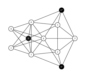
Figure 1: Graph for a quantum code that is locally Clifford equivalent to the Gottesman [[8,3,3]]-code.

IV.2.4 Step four

To verify that the code associated with the $\left[\left[8,3,3\right]\right]$ graph corrects any one error, we must verify that the code detects any two errors. Specifically, for every two-element error configuration $E$, we must have

$$\Gamma_{X\cup E}^{I}d^{X\cup E}=0\Rightarrow d^{X\cup E}=0\text{,}$$ (53)

where $I\overset{\text{def}}{=}Y\backslash E$ with $E$, $X$, $Y$ denoting the error configuration, the input vertices, and the output vertices, respectively. In our specific case, we have

$$X\overset{\text{def}}{=}\left\{0\text{, }0^{\prime}\text{, }0^{\prime\prime}\right\}\text{, }Y\overset{\text{def}}{=}\left\{1\text{,..., }8\right\}\text{, }E\overset{\text{def}}{=}\left\{e_{1}\text{, }e_{2}\right\}\text{, and }X\cup E\overset{\text{def}}{=}\left\{0\text{, }0^{\prime}\text{, }0^{\prime\prime}\text{, }e_{1}\text{, }e_{2}\right\}\text{,}$$ (54)

where $e_{1,2}\in\left\{1\text{,..., }8\right\}$ and the number of two-element error configurations (that is, the number of sets $X\cup E$) is $\binom{8}{2}=28$. Observe that when applying Eq. (53), the input vertices play exactly the same role as an error. For a fixed integration vertex $y\in I\overset{\text{def}}{=}Y\backslash E$ and a given two-element error configuration $E$, the condition $\Gamma_{X\cup E}^{I}d^{X\cup E}=0$ is a set of $\left|I\right|=\left|Y\right|-\left|E\right|=8-2=6$-equations. In total, we have to verify $28$-systems of linear algebraic equations with each system defined by $6$-equations. In particular, for each $y_{\ast}$ we have to sum the $d_{x}$ for all vertices $x\in X\cup E$. For the sake of clarity, consider the two-error configuration $E=\left\{0\text{, }0^{\prime}\text{, }0^{\prime\prime}\text{, }5\text{, }7\right\}$. The corresponding linear system specified by six constraint equations is given by,

$$\left\{\begin{array}[c]{c}y_{\ast}=1:d_{0}+d_{7}=0\\ y_{\ast}=2:d_{0}+d_{0^{\prime}}+d_{5}+d_{7}=0\\ y_{\ast}=3:d_{0}+d_{0^{\prime\prime}}+d_{5}=0\\ y_{\ast}=4:d_{0^{\prime}}+d_{0^{\prime\prime}}+d_{5}+d_{7}=0\\ y_{\ast}=6:d_{0}+d_{0^{\prime\prime}}+d_{7}=0\\ y_{\ast}=8:d_{0}+d_{7}=0\end{array}\right.\text{.}$$ (55)

From simple algebraic manipulations, it can be shown that the system in Eq. (55) yields $d_{0}=d_{0^{\prime}}=d_{0^{\prime\prime}}=d_{5}=d_{7}=0$. Therefore, the two-error configurations $\left\{0\text{, }0^{\prime}\text{, }0^{\prime\prime}\text{, }5\text{, }7\right\}$ is detectable. Following this line of reasoning, it can be verified that any of the $\binom{8}{2}$ graphical two-error configurations $\left\{0\text{, }0^{\prime}\text{, }0^{\prime\prime}\text{, }e_{1}\text{, }e_{2}\right\}$ with $e_{1,2}\in\left\{1\text{,..., }8\right\}$ is detectable. Thus, the code corrects any single-qubit error.

V Concluding remarks

In this article, we proposed a systematic scheme for the construction of graphs with both input and output vertices associated with arbitrary binary stabilizer codes. The scheme is characterized by three main steps: first, the stabilizer code is realized as a CWS quantum code; second, the canonical form of the CWS code is uncovered; third, the input vertices are attached to the graphs. To verify the effectiveness of the scheme, we implemented the Gottesman $\left[\left[8\text{, }3\text{, }3\right]\right]$ stabilizer code characterized by multi-qubit encoding operators for the error correction of single amplitude damping errors. In particular, the error-correcting capabilities of the $\left[\left[8\text{, }3\text{, }3\right]\right]$ eight-qubit quantum stabilizer code is verified in graph-theoretic terms as originally advocated by Schlingemann and Werner.

Our two main contributions proposed in this article can be stated as follows:

• First, our investigation features robust pedagogical and explanatory value. Indeed, the construction of graphs not only occurs via a novel alternative scheme, but is also illustrated in a step-by-step fashion via explicit analytical computations. This step-by-step procedure is helpful for three reasons. i) First, it highlights one of the main consequence of the choices made during explicit application of the scheme, that is to say, different choices lead to the emergence of non-isomorphic graphs which yield equivalent graphical quantum codes that are all suitable representations of the same stabilizer code as originally pointed out by Grassl et al. in Refs. markus ; markus1 . Indeed, while each graph state corresponds uniquely to a graph, two graph states can be equivalent under local unitary transformations and yield two, non-isomorphic, distinct graphs. Therefore, as previously mentioned, there could be non-isomorphic graphs which all yield graph codes that are distinct suitable representations of the very same stabilizer code. For an interesting and relatively recent discussion on the relation between graph states and graph codes, we refer to Ref. hwang16 . ii) Second, it provides a unifying framework to construct graphical depictions of known binary stabilizer codes, with the former being sparsely available in the current literature. During this process, we are also able to provide new graphical depictions in the presence of both single and multi-qubit encodings. iii) Third, it allows to reconsider the importance of the original graphical quantum error correction conditions after establishing the clear connection between stabilizer and graph codes.

• Second, the algorithmic construction of our proposed scheme also offers pure theoretical and conceptual value. Indeed, we show how the hybrid logical blending of different results- the CWS formalism cross , the algorithmic procedure to transform a stabilizer state into a graph state bart , and the concise link between graph codes and stabilizer codes dirk - lead to an alternative method for constructing graphs of binary stabilizer codes. In the process, we argue that all these different results become even more relevant and powerful within our scheme since, among other things, they solve an old problem in a new fashion. In particular, i) the Cross et al. CWS formalism provides a unifying framework for QEC code design. Once the stabilizer code is realized as a CWS code, such a code is locally equivalent to another CWS code in its standard form. In order to find such a standard form, a suitable local Clifford (unitary) transformation has to be identified. The CWS formalism does not address this specific issue. Nevertheless, identifying the standard form of a CWS code can be especially useful when regarding stabilizer codes as graph codes, and vice-versa. ii) To determine the standard form of a CWS code corresponding to a given stabilizer code, we exploit the algorithmic procedure proposed by Van den Nest et al. for transforming any binary quantum stabilizer state into a graph state. We adapt this algorithmic procedure to the CWS language by replacing the generator matrix of the stabilizer state with the codeword stabilizer of the CWS code that realizes the binary stabilizer code whose depiction is being investigated. At the end of this step, one has the adjacency matrix $\Gamma$ of the graph with only output vertices for the stabilizer code associated with a suitable isotropic subspace. The work by Van den Nest et al. is not concerned with the issue of finding the extended graph of the stabilizer code, that is, the graph with both input and output vertices (to which, we associate the coincidence matrix $\Xi$). iii) To find the extended graph of a $\left[\left[n\text{, }k\text{, }d\right]\right]$ binary stabilizer code, we need to attach input vertices to the graph associated with $\Gamma$. To achieve this goal, we take advantage of a finding attributed to Schlingemann: a graph code with associated extended graph including both input and output vertices is equivalent to stabilizer codes associated with a suitable isotropic subspace. Since each stabilizer code can be realized as a graph code and vice-versa, we exploit the afore-mentioned finding in reverse to obtain $\Xi$. iv) After completing the steps described above, we are able to construct a graph for arbitrary stabilizer codes. Then, the original graphical quantum error correction and detection conditions proposed by Schlingemann and Werner in Ref. werner can be re-examined and their usefulness can be tested.

The scheme proposed in this article is limited to binary stabilizer codes. How do we begin addressing from a graph-theoretic perspective non-binary beigi2 and continuous-variable (CV) zang5 codes? What about non-additive codes? We believe that the extension of our proposed scheme to codes of this kind will likely pose a highly non-trivial challenge. Despite its evident limitations, we view our work as a serious effort that not only expands the interplay among several theoretical formalisms werner ; dirk ; bart ; cross , but it also contributes in a non-trivial manner to the rich relationship between graph theory and stabilizer formalism in quantum information guhne17 ; adcock20 , with special relevance to quantum error correction wagner18 . Finally, in view of the progressive advances in the field, we are confident that the generalization of our current work could be readily achieved with concerted and persistent effort.

Appendix A Technical concepts

In this Appendix, we present a brief review of several technical concepts. First, the notions of graphs, graph states and graph codes are introduced. Second, local Clifford transformations on graph states and local complementations on graphs are briefly presented.

A.1 Graphs, graph states, and graph codes

Graphs. A graph $G\overset{\text{def}}{=}G\left(V\text{, }E\right)$ is specified by a set $V$ of $n$ vertices together with a set of edges $E$, the latter being characterized by the adjacency matrix $\Gamma$ die ; west ; wilson . The matrix $\Gamma$ is an $n\times n$ symmetric matrix with vanishing diagonal elements, where $\Gamma_{ij}=1$ if vertices $i$, $j$ are connected and $\Gamma_{ij}=0$ otherwise. The neighborhood of a vertex $i$ corresponds to the set of all vertices $v\in V$ that are connected to $i$ and is defined by $N_{i}\overset{\text{def}}{=}\left\{v\in V:\Gamma_{iv}=1\right\}$. When the vertices $a$, $b\in V$ coincide with the end points of an edge, they are said to be adjacent. An $\left\{a\text{, }c\right\}$ path is an ordered list of vertices $a=a_{1}$, $a_{2}$,…, $a_{n-1}$, $a_{n}=c$, such that $\forall i$, $a_{i}$ and $a_{i+1}$ are adjacent. A connected graph is one that has an $\left\{a\text{, }c\right\}$ path for any two $a$, $c\in V$, otherwise the graph is disconnected. A vertex represents a physical system, e.g. a qubit (two-dimensional Hilbert space), qudit ($d$-dimensional Hilbert space, for an example of quantum error correction with qudits, we refer to cafaro12 ), or continuous variables (CV) (continuous Hilbert space, for an example of quantum error correction with CVs, we refer to ralph11 ). An edge between two vertices represents the physical interaction between the corresponding systems. In what follows, we will exclusively consider simple graphs. Simple graphs are those that contain neither loops (i.e. edges connecting vertices with itself) nor multiple edges. For the sake of completeness, we remark that is is possible to make a distinction between different types of vertices. For example, one can assign some vertices as inputs, and others as outputs.

Graph states. Graph states hans describe multipartite entangled states which play a key-role in the graphical construction of QECCs codes and additionally, play an important role in quantum secret sharing damian2008 which to a certain extent, is equivalent to error correction anne2013 . For a recent experimental demonstration of a graph state quantum error correcting code, we refer the reader to damian2014 . Consider a system of $n$ qubits that are labeled by the $n$ vertices in $V$. Furthermore, denote by $I^{i}$, $X^{i}$, $Y^{i}$, $Z^{i}$ (or equivalently, $X^{i}\equiv\sigma_{x}^{i}$, $Y^{i}\equiv\sigma_{y}^{i}$, $Z^{i}\equiv\sigma_{z}^{i}$) the identity matrix and the three Pauli operators acting on the qubit $i\in V$. The $n$-qubit graph state $\left|G\right\rangle$ associated with the graph $G$ is defined by hein ,

$$\left|G\right\rangle\overset{\text{def}}{=}{\displaystyle\prod\limits_{\Gamma_{ij}=1}}\mathcal{U}_{ij}\left|+\right\rangle_{x}^{V}=\frac{1}{\sqrt{2^{n}}}{\displaystyle\sum\limits_{\vec{\mu}=\mathbf{0}}^{\mathbf{1}}}\left(-1\right)^{\frac{1}{2}\vec{\mu}\cdot\Gamma\cdot\vec{\mu}}\left|\vec{\mu}\right\rangle_{z}\text{,}$$ (56)

where $\left|+\right\rangle_{x}^{V}$ is the joint $+1$ eigenstate of $X^{i}$ with $i\in V$, and $\mathcal{U}_{ij}$ is the controlled phase gate between qubits $i$ and $j$ given by,

$$\mathcal{U}_{ij}\overset{\text{def}}{=}\frac{1}{2}\left[I+Z_{i}+Z_{j}-Z_{i}Z_{j}\right]\text{,}$$ (57)

and $\left|\vec{\mu}\right\rangle_{z}$ being the joint eigenstate of $Z^{i}$ with $i\in V$ and $\left(-1\right)^{\mu_{i}}$ as eigenvalues. The graph-state basis of the $n$-qubit Hilbert space $\mathcal{H}_{2}^{n}$ is given by $\left\{\left|G^{C}\right\rangle\overset{\text{def}}{=}Z^{C}\left|G\right\rangle\right\}$, where $C$ is an element of the set of all subsets of $V$ denoted by $2^{V}$. A collection of subsets $\left\{C_{1}\text{,..., }C_{K}\right\}$ specifies a $K$-dimensional subspace of $\mathcal{H}_{2}^{n}$ that is spanned by the graph-state basis $\left\{\left|G^{C_{i}}\right\rangle\right\}$ with $i=1$,…, $K$. The graph state $\left|G\right\rangle$ is the unique joint $+1$ eigenstate of the $n$-vertex stabilizers $\mathcal{G}_{i}$ with $i\in V$ defined as hein ,

$$\mathcal{G}_{i}\overset{\text{def}}{=}X^{i}Z^{N_{i}}\overset{\text{def}}{=}X^{i}{\displaystyle\prod\limits_{j\in N_{i}}}Z^{j}\text{.}$$ (58)

Graph codes. A graph code, first introduced in the field of QEC in werner and later reformulated in the graph state formalism hein , is defined to be one in which a graph $G$ is given and the codespace (or coding space) is spanned by a subset of the graph state basis. These states are regarded as codewords, although we recall that what is significant from the perspective of the QEC properties is the subspace they span, not the codewords themselves robert98 .

A.2 Local Clifford transformations and local complementations

A.2.1 Transformations on quantum states 

The Clifford group $\mathcal{C}_{n}$ is the normalizer of the Pauli group $\mathcal{P}_{\mathcal{H}_{2}^{n}}$ in $\mathcal{U}\left(2^{n}\right)$, i.e. it is the group of unitary operators $U$ satisfying $U\mathcal{P}_{\mathcal{H}_{2}^{n}}U^{\dagger}=\mathcal{P}_{\mathcal{H}_{2}^{n}}$. The local Clifford group $\mathcal{C}_{n}^{l}$ is a subgroup of $\mathcal{C}_{n}$ and is comprised of all $n$-fold tensor products of elements in $\mathcal{C}_{1}$. The Clifford group is generated by a simple set of quantum gates, namely the Hadamard gate $H$, the phase gate $P$ and the CNOT gate $U_{\text{CNOT}}$ gaitan . Using the well-known representations of the Pauli matrices in the computational basis, it is straightforward to verify that the action of $H$ on such matrices reads,

$$\sigma_{x}\rightarrow H\sigma_{x}H^{\dagger}=\sigma_{z}\text{, }\sigma_{y}\rightarrow H\sigma_{y}H^{\dagger}=-\sigma_{y}\text{, }\sigma_{z}\rightarrow H\sigma_{z}H^{\dagger}=\sigma_{x}\text{.}$$ (59)

The action of the phase gate $P$ on $\sigma_{x}$, $\sigma_{y}$ and $\sigma_{z}$ is given by,

$$\sigma_{x}\rightarrow P\sigma_{x}^{\dagger}P=\sigma_{y}\text{, }\sigma_{y}\rightarrow P\sigma_{y}^{\dagger}P=-\sigma_{x}\text{, }\sigma_{z}\rightarrow P\sigma_{z}^{\dagger}P=\sigma_{z}\text{.}$$ (60)

Finally, the CNOT gate leads to the following transformations rules,

$$\sigma_{x}\otimes I \rightarrow U_{\text{CNOT}}\left(\sigma_{x}\otimes I\right)U_{\text{CNOT}}^{\dagger}=\sigma_{x}\otimes\sigma_{x}\text{, }I\otimes\sigma_{x}\rightarrow U_{\text{CNOT}}\left(I\otimes\sigma_{x}\right)U_{\text{CNOT}}^{\dagger}=I\otimes\sigma_{x}\text{,}$$

$$\sigma_{z}\otimes I \rightarrow U_{\text{CNOT}}\left(\sigma_{z}\otimes I\right)U_{\text{CNOT}}^{\dagger}=\sigma_{z}\otimes I\text{, }I\otimes\sigma_{z}\rightarrow U_{\text{CNOT}}\left(I\otimes\sigma_{z}\right)U_{\text{CNOT}}^{\dagger}=\sigma_{z}\otimes\sigma_{z}\text{.}$$ (61)

Observe that the CNOT gate propagates bit flip errors from the control to the target, and phase errors from the target to the control. As a side remark, we stress that another useful two-qubit gate is the controlled-phase gate $U_{\text{CP}}\overset{\text{def}}{=}\left(I\otimes H\right)U_{\text{CNOT}}\left(I\otimes H\right)$. The controlled-phase gate has the following action on the generators of $\mathcal{P}_{\mathcal{H}_{2}^{2}}$,

$$\sigma_{x}\otimes I \rightarrow U_{\text{CP}}\left(\sigma_{x}\otimes I\right)U_{\text{CP}}^{\dagger}=\sigma_{x}\otimes\sigma_{z}\text{, }I\otimes\sigma_{x}\rightarrow U_{\text{CP}}\left(I\otimes\sigma_{x}\right)U_{\text{CP}}^{\dagger}=\sigma_{z}\otimes\sigma_{x}\text{,}$$

$$\sigma_{z}\otimes I \rightarrow U_{\text{CP}}\left(\sigma_{z}\otimes I\right)U_{\text{CP}}^{\dagger}=\sigma_{z}\otimes I\text{, }I\otimes\sigma_{z}\rightarrow U_{\text{CP}}\left(I\otimes\sigma_{z}\right)U_{\text{CP}}^{\dagger}=I\otimes\sigma_{z}\text{.}$$ (62)

It is evident that a controlled-phase gate does not propagate phase errors, though a bit-flip error on one qubit spreads to a phase error to another qubit. It is worth noting that a unitary operator $U$ that fixes the stabilizer group $\mathcal{S}_{\text{stabilizer}}$ (we refer to daniel-phd for a detailed exposition of the quantum stabilizer formalism in QEC) of a quantum stabilizer code $\mathcal{C}_{\text{stabilizer}}$ under conjugation is an encoded operation. In other words, $U$ is an encoded operation that maps codewords to codewords whenever $U\mathcal{S}_{\text{stabilizer}}U^{\dagger}=\mathcal{S}_{\text{stabilizer}}$. In particular, if $\mathcal{S}^{\prime}\overset{\text{def}}{=}U\mathcal{S}U^{\dagger}$ (every element of $\mathcal{S}^{\prime}$ can be written as $UsU^{\dagger}$ for some $s\in\mathcal{S}$) and $\left|c\right\rangle$ is a codeword stabilized by every element in $\mathcal{S}$, then $\left|c^{\prime}\right\rangle=U\left|c\right\rangle$ is stabilized by every stabilizer element in $\mathcal{S}^{\prime}$.

A.2.2 Transformations on graphs

If there exists a local unitary (LU) transformation $U$ such that $U\left|G\right\rangle=\left|G^{\prime}\right\rangle$, the states $\left|G\right\rangle$ and $\left|G^{\prime}\right\rangle$ will have the same entanglement properties. If $\left|G\right\rangle$ and $\left|G^{\prime}\right\rangle$ are graph states, then we say that their corresponding graphs $G$ and $G^{\prime}$ will represent equivalent quantum codes, with the same distance, weight distribution, and other properties. Ascertaining whether two graphs are LU-equivalent is a difficult task, but a sufficient condition for equivalence was given in hein . Let the graphs $G\overset{\text{def}}{=}G\left(V\text{, }E\right)$ and $G^{\prime}\overset{\text{def}}{=}G^{\prime}\left(V\text{, }E^{\prime}\right)$ on $n$ vertices correspond to the $n$-qubit graph states $\left|G\right\rangle$ and $\left|G^{\prime}\right\rangle$. We define the two $2\times 2$ unitary matrices,

$$\tau_{x}\overset{\text{def}}{=}\sqrt{-i\sigma_{x}}=\frac{1}{\sqrt{2}}\left(\begin{array}[c]{cc}-1&i\\ i&-1\end{array}\right)\text{ and }\tau_{z}\overset{\text{def}}{=}\sqrt{i\sigma_{z}}=\left(\begin{array}[c]{cc}\omega&0\\ 0&\omega^{3}\end{array}\right)\text{,}$$ (63)

with $\omega^{4}=i^{2}=-1$, where $\sigma_{x}$ and $\sigma_{z}$ are Pauli matrices. Given a graph $G\overset{\text{def}}{=}G\left(V=\left\{0\text{,..., }n-1\right\}\text{, }E\right)$ corresponding to the graph state $\left|G\right\rangle$, we define a local unitary transformation $U_{a}$,

$$U_{a}\overset{\text{def}}{=}{\displaystyle\bigotimes\limits_{i\in N_{a}}}\tau_{x}^{\left(i\right)}{\displaystyle\bigotimes\limits_{i\notin N_{a}}}\tau_{z}^{\left(i\right)}\text{,}$$ (64)

where $a\in V$ is any vertex, $N_{a}\subset V$ is the neighborhood of $a$, and $\tau_{x}^{\left(i\right)}$ means that the transform $\tau_{x}$ should be applied to the qubit corresponding to vertex $i$. Given a graph $G$, if there exists a finite sequence of vertices $\left(u_{0}\text{,..., }u_{k-1}\right)$ such that $U_{u_{k-1}}$…$U_{u_{0}}\left|G\right\rangle=\left|G^{\prime}\right\rangle$, then $G$ and $G^{\prime}$ are LU-equivalent hein . It was discovered by Hein et al. and by Van den Nest et al. that the sequence of transformations mapping $\left|G\right\rangle$ to $\left|G^{\prime}\right\rangle$ can equivalently be expressed as a sequence of simple graph operations taking $G$ to $G^{\prime}$. In particular, it was shown in bart that a graph $G$ uniquely determines a graph state $\left|G\right\rangle$ while two graph states ($\left|G_{1}\right\rangle$ and $\left|G_{2}\right\rangle$) determined by two graphs ($G_{1}$ and $G_{2}$) are equivalent up to some local Clifford transformations if and only if these two graphs are related to each other by local complementations (LCs). The concept of LCs was originally introduced by Bouchet in france . A LC of a graph on a vertex $v$ refers to the operation in the neighborhood of $v$ whereby we connect all disconnected vertices and simultaneously disconnect all the connected vertices. All graphs up to $12$ vertices have been classified under LCs and graph isomorphisms parker . It is abundantly clear that the relationship between graphs and quantum codes can be rather complicated since one graph may provide non-equivalent codes and different graphs may provide equivalent codes. It has been established however, that the family of codes given by a graph is equivalent to the family of codes given by a local complementation of that graph.

As mentioned earlier, unitary operations $U$ in the local Clifford group $\mathcal{C}_{n}^{l}$ act on graph states $\left|G\right\rangle$. There also exists graph theoretic rules (i.e. transformations acting on graphs), which correspond to local Clifford operations. These operations generate the orbit of any graph state under local Clifford operations. The LC orbit of a graph $G$ is the set of all non-isomorphic graphs, including $G$ itself, that can be transformed into $G$ by means of any sequence of LCs and vertex permutations. The transformation laws for a graph state $\left|G\right\rangle$ and a graph stabilizer $\mathcal{S}_{\Gamma}$ under local unitary transformations $U$ read,

$$\left|G\right\rangle\rightarrow\left|G^{\prime}\right\rangle=U\left|G\right\rangle\text{ and }\mathcal{S}_{\Gamma}\rightarrow\mathcal{S}_{\Gamma^{\prime}}=U\mathcal{S}_{\Gamma}U^{\dagger}\text{,}$$ (65)

respectively. Neglecting overall phases, it can be shown that local Clifford operations $U\in\mathcal{C}_{n}^{l}$ are equivalent to the symplectic transformations $Q$ of $\mathbb{Z}_{2}^{2n}$ which preserve the symplectic inner product moor . Therefore, the $\left(2n\times 2n\right)$-matrices $Q$ satisfy the relation $Q^{T}PQ=P$ where the symbol “$T$” denotes the transpose operation and $P$ is the $\left(2n\times 2n\right)$-matrix that defines a symplectic inner product in $\mathbb{Z}_{2}^{2n}$, namely

$$P\overset{\text{def}}{=}\left(\begin{array}[c]{cc}0&I\\ I&0\end{array}\right)\text{.}$$ (66)

Furthermore, since local Clifford operations act on each qubit separately, they have the additional block structure

$$Q\overset{\text{def}}{=}\left(\begin{array}[c]{cc}A&B\\ C&D\end{array}\right)\text{,}$$ (67)

where the $\left(n\times n\right)$-blocks $A$, $B$, $C$, $D$ are diagonal. It was shown in bart that each binary stabilizer state is equivalent to a graph state. In particular, each graph state characterized by the adjacency matrix $\Gamma$ corresponds to a stabilizer matrix $\mathcal{S}_{b}\overset{\text{def}}{=}\left(\Gamma\left|I\right.\right)$ and transpose stabilizer (generator matrix) $\mathcal{T}\overset{\text{def}}{=}\mathcal{S}_{b}^{T}=\binom{\Gamma}{I}$. The generator matrix $\binom{\Gamma^{\prime}}{I}$ for a graph state with adjacency matrix $\Gamma^{\prime}$ reads,

$$\binom{\Gamma}{I}\rightarrow\binom{\Gamma^{\prime}}{I}=\left(\begin{array}[c]{cc}A&B\\ C&D\end{array}\right)\binom{\Gamma}{I}\left(C\Gamma+D\right)^{-1}\text{,}$$ (68)

where,

$$\Gamma^{\prime}\overset{\text{def}}{=}Q\left(\Gamma\right)=\left(A\Gamma+B\right)\left(C\Gamma+D\right)^{-1}\text{.}$$ (69)

Observe that in order to have properly defined generator matrices in Eq. (68), $C\Gamma+D$ must be non-singular and $\Gamma^{\prime}$ must have vanishing diagonal elements. The graphical analogue of the transformation law in Eq. (69) was provided in bart . Before stating this result however, the introduction of additional terminology is required.

Two vertices $i$ and $j$ of a graph $G=G\left(V\text{, }E\right)$ are called adjacent vertices, or neighbors, if $\left\{i\text{, }j\right\}\in E$. The neighborhood $N\left(i\right)\subseteq V$ of a vertex $i$ is the set of all neighbors of $i$. A graph $G^{\prime}=G^{\prime}\left(V^{\prime}\text{, }E^{\prime}\right)$ which satisfies $V^{\prime}\subseteq V$ and $E^{\prime}\subseteq E$ is a subgraph of $G$ and one writes $G^{\prime}\subseteq G$. For a subset $A\subseteq V$ of vertices, the induced subgraph $G\left[A\right]\subseteq G$ is the graph with vertex set $A$ and edge set $\left\{\left\{i\text{, }j\right\}\in E:i\text{, }j\in A\right\}$. If $G$ has an adjacency matrix $\Gamma$, its complement $G^{\text{c}}$ is the graph with adjacency matrix $\Gamma+\mathbf{I}$, where $\mathbf{I}$ is the $\left(n\times n\right)$-matrix whose elements are all ones, except for the diagonal entries which are zeros. For each vertex $i=1$,…, $n$, a local complementation $g_{i}$ sends the $n$-vertex graph $G$ to the graph $g_{i}\left(G\right)$ which is obtained by replacing the induced subgraph $G\left[N\left(i\right)\right]$ by its complement. In other words,

$$\Gamma\rightarrow\Gamma^{\prime}\equiv g_{i}(\Gamma)\overset{\text{def}}{=}\Gamma+\Gamma\Lambda_{i}\Gamma+\Lambda^{\left(i\right)}\text{,}$$ (70)

where $\Lambda_{i}$ has a $1$ on the $i$th diagonal entry, zeros elsewhere and $\Lambda^{\left(i\right)}$ is a diagonal matrix such that it yields zeros on the diagonal of $g_{i}(\Gamma)$. Finally, the graphical analogue of Eq. (69) becomes,

$$Q_{i}\left(\Gamma\right)=g_{i}(\Gamma)\text{,}$$ (71)

with,

$$Q_{i}\overset{\text{def}}{=}\left(\begin{array}[c]{cc}I&\text{{diag}}\left(\Gamma_{i}\right)\\ \Lambda_{i}&I\end{array}\right)\text{,}$$ (72)

where diag$\left(\Gamma_{i}\right)\overset{\text{def}}{=}$diag$\left(\Gamma_{i1}\text{,..., }\Gamma_{in}\right)$. In our proposed scheme, the matrix $Q_{i}$ in Eq. (72) represents a transformation that links two distinct binary vector representations $\left\{v_{S_{k}}\right\}$ and $\left\{v_{S_{k}^{\prime}}\right\}\overset{\text{def}}{=}\left\{Q_{i}v_{S_{k}}\right\}$ of operators $\left\{S_{k}\right\}$ and $\left\{S_{k}^{\prime}\right\}\overset{\text{def}}{=}\left\{US_{k}U^{\dagger}\right\}$ that belong to two distinct codeword stabilizers $\mathcal{S}_{\text{CWS}}$ and $\mathcal{S}_{\text{CWS}}^{\prime}$ associated to graphs with adjacency matrices $\Gamma$ and $\Gamma^{\prime}\equiv g_{i}(\Gamma)$, respectively. Observe that by substituting (72) into (69) and using (70), Eq. (71) gives

$$Q_{i}\left(\Gamma\right)=g_{i}(\Gamma)\Leftrightarrow\Gamma+\Gamma\Lambda_{i}\Gamma+\Lambda^{\left(i\right)}=\Gamma+\Gamma\Lambda_{i}\Gamma+\left[\text{{diag}}\left(\Gamma_{i}\right)+\text{{diag}}\left(\Gamma_{i}\right)\Lambda_{i}\Gamma\right]\text{,}$$ (73)

that is,

$$\Lambda^{\left(i\right)}=\text{{diag}}\left(\Gamma_{i}\right)+\text{{diag}}\left(\Gamma_{i}\right)\Lambda_{i}\Gamma\text{.}$$ (74)

The translation of the action of local Clifford operations on graph states into the action of local complementations on graphs as presented in Eq. (71) is a major achievement of bart .