Spectral branch points of the Bloch-Torrey operator

Abstract

We investigate the peculiar feature of non-Hermitian operators, namely, the existence of spectral branch points (also known as exceptional or level crossing points), at which two (or many) eigenmodes collapse onto a single eigenmode and thus loose their completeness. Such branch points are generic and produce non-analyticities in the spectrum of the operator, which, in turn, result in a finite convergence radius of perturbative expansions based on eigenvalues and eigenmodes that can be relevant even for Hermitian operators. We start with a pedagogic introduction to this phenomenon by considering the case of $2\times 2$ matrices and explaining how the analysis of more general differential operators can be reduced to this setting. We propose an efficient numerical algorithm to find spectral branch points in the complex plane. This algorithm is then employed to show the emergence of spectral branch points in the spectrum of the Bloch-Torrey operator $-\nabla^{2}-igx$, which governs the time evolution of the nuclear magnetization under diffusion and precession. We discuss their mathematical properties and physical implications for diffusion nuclear magnetic resonance experiments in general bounded domains.

1 Introduction

Hermitian (or self-adjoint) operators play the central role in quantum and classical physics by governing a broad variety of natural phenomena, such as diffusion, wave propagation, or evolution of a quantum state. Spectral properties of these operators have been thoroughly investigated [1, 2, 3, 4, 5, 6]. In many practically relevant cases, a Hermitian operator has a discrete (or pure point) spectrum of real eigenvalues, while the associated eigenfunctions (also called eigenmodes or eigenvectors) form a complete orthogonal basis in the underlying functional space. As an expansion of a function on that basis reduces the operator to a multiplication operator, the related spectral expansions are commonly used, e.g., in quantum mechanics and in stochastic theory. Even though Hermitian operators form an “exceptional” set of operators (in the same sense as real numbers are “exceptional” among complex numbers), they are most often encountered in applications. In turn, more general non-Hermitian operators that may possess a discrete, continuous or even empty spectrum, present a richer variety of spectral properties [7]. Even if the spectrum is discrete, some eigenvalues may coalesce at specific branch points (also known as exceptional points or level crossing points), at which the completeness of eigenmodes is generally lost, thus failing conventional spectral expansions [2, 4]. As spectral branch points lie in the complex plane, this failure can be unnoticed but still relevant even for Hermitian operators. For instance, Bender and Wu studied an anharmonic (quartic) quantum oscillator governed by the Hamiltonian ${\mathcal{B}}(g)=-d^{2}/dx^{2}+x^{2}+gx^{4}$ and discovered an infinity of branch points that cause divergence of the perturbation series in powers of $g$ for the ground-energy state [8] (see [9, 10, 11, 12] for further details and extensions). Even if the parameter $g$ is real and the operator ${\mathcal{B}}(g)$ is thus Hermitian, the accumulation of branch points near the origin prohibits a perturbative approach to this problem. In other words, the existence of branch points may crucially affect the spectral expansions of Hermitian operators as well.

Peculiar properties of spectral branch points have been studied for various non-Hermitian operators (see, e.g., [13, 14, 15, 16, 17, 18, 19, 20, 21, 22, 23, 24] and references therein). While a branch point often involves two eigenvalues, higher-order branch points offer even richer mathematical structure and physical properties. For instance, Jin considered two symmetrically coupled asymmetric dimers and discussed phase transitions when encircling the exceptional points [25]. Hybrid exceptional points that exhibit different dispersion relations along different directions in the parameter space, were studied on a two-state system of coupled ferromagnetic waveguides with a bias magnetic field [26], while high-order exceptional points in supersymmetric arrays of coupled resonators or waveguides under a gradient gain and loss were discussed in [27] (see also [28, 29]).

Apart from being an object of intensive mathematical investigations, spectral branch points have recently found numerous physical implications. For instance, Xu et al. reported an experimental realization of the transfer of energy between two vibrational modes of a cryogenic optomechanical device that arises from the presence of an exceptional point in the spectrum of that device [30]. More generally, a dynamical encircling of an exceptional point in parameter space may lead to the accumulation of a geometric phase and thus realize a robust and asymmetric switch between different modes, as shown experimentally for scattering through a two-mode waveguide with suitably designed boundaries and losses [31] (see also [32, 33]). Yoon et al. constructed two coupled silicon-channel waveguides with photonic modes that transmit through time-asymmetric loops around an exceptional point in the optical domain, taking a step towards broadband on-chip optical devices based on non-Hermitian topological dynamics [34]. Along the same line, Schumer et al. designed a structure that allows the lasing mode to encircle a non-Hermitian exceptional point so that the resulting state transfer reflects the unique topology of the associated Riemann surfaces associated with this singularity [35]. This approach aimed to provide a route to developing versatile mode-selective active devices and to shed light on the interesting topological features of exceptional points. Hassan et al. theoretically analyzed the behavior of two coupled states whose dynamics are governed by a non-Hermitian Hamiltonian undergoing cyclic variations in the diagonal terms [36]. They obtained analytical solutions that explain the asymmetric conversion into a preferred mode and the chiral nature of this mechanism. However, the latest experiments on a fibre-based photonic emulator showed that chiral state transfer can be realized without encircling an exceptional point and seems to be mostly attributed to the non-trivial landscape of the energy Riemann surfaces [37].

In this paper, we investigate the spectral branch points of the Bloch-Torrey differential operator $\mathcal{B}(g)=-\nabla^{2}-igx$, acting on a subspace of square-integrable functions on a bounded Euclidean domain $\Omega\subset{\mathbb{R}}^{d}$ [38]. For $g\in{\mathbb{R}}$, this non-Hermitian operator describes diffusion and precession of nuclear spins under a magnetic field gradient [39, 40, 41, 42, 43, 44, 45, 46]. While spectral properties of the Bloch-Torrey operator have been studied in the past [47, 48, 49, 50, 51, 52, 53, 54, 55, 56, 57], a systematic analysis of its branch points is still missing. In fact, we are aware of a single work by Stoller et al. [47], who discussed spectral branch points of the Bloch-Torrey operator on an interval with reflecting endpoints. In addition, few numerical examples of branch points for some planar domains were given in [56]. We start with a pedagogic introduction to spectral branch points in Sec. 2 by considering a basic example of $2\times 2$ matrices (this introductory section may be skipped by an expert reader). Section 3 describes our main results. We first look at the spectral branch points of the Bloch-Torrey operator $\mathcal{B}(g)$ in parity-symmetric domains. In order to deal with arbitrary domains, we present a numerical algorithm for determining spectral branch points in the complex plane. In particular, we illustrate that branch points generally lie outside the real axis when the parity symmetry is lost. In Sec. 4, we outline how the presence of branch points implies a finite convergence radius of perturbative expansions. In particular, we estimate this radius for the Bloch-Torrey operator in two domains and discuss its immediate consequences for diffusion nuclear magnetic resonance (NMR) experiments. Section 5 concludes the paper with a summary of main results and future perspectives.

2 Pedagogic introduction to spectral branch points

In this section, we provide a pedagogic introduction to spectral branch points from a general point of view for non-expert readers. This is a simplified sketch of classical descriptions that can be found in most textbooks on spectral theory [2, 3, 4, 7, 58].

Let $\mathcal{B}(g)$ denote a linear operator on a vector space $E$ that depends analytically on a complex parameter $g$. We assume that $\mathcal{B}(g)$ has a discrete spectrum for any $g\in\mathbb{C}$, and $\{\lambda_{n}(g)\}$ denotes the set of its eigenvalues, i.e., the poles of the resolvent $(\mathcal{B}(g)-\lambda\mathcal{I})^{-1}$. Intuitively, one can expect that each $\lambda_{n}(g)$ depends “smoothly” on $g$, except for some points, at which two (or many) eigenvalues coincide. For a Hermitian operator, crossing of eigenvalues does not alter the spectral properties and does keep analytical dependence on $g$. In contrast, crossing of two eigenvalues of a non-Hermitian operator at some point $g_{0}$ results in a non-analytical dependence on $g$ in a vicinity of $g_{0}$. Moreover, the behavior of the corresponding eigenmodes drastically changes at $g_{0}$, as described below.

2.1 Spectral branch points as complex branch points of a multi-valued function

The spectrum $\{\lambda_{n}(g)\}$ of the operator $\mathcal{B}(g)$ is often obtained by solving an equation of the form

$$F(\lambda,g)=0,$$ (1)

where $F$ is an analytical function of $\lambda$ and $g$. For a matrix, this function is simply its characteristic polynomial, while a differential operator generally yields a transcendental function $F$. For example, the operator $\mathcal{B}=-\partial_{x}^{2}+g$ on the interval $(0,1)$ with Dirichlet boundary condition leads to the spectral equation: $F(\lambda,g)=\sin(\sqrt{\lambda-g})=0$.

To illustrate how branch points may result from the spectral equation (1), let us consider a simple example:

$$F(\lambda,g)=\lambda^{2}-g=0\;.$$ (2)

This equation can be inverted to obtain $\lambda$ as a function of $g$ but the inversion of the square function makes $\lambda(g)$ a multi-valued function with two possible values (i.e., two sheets in the complex plane):

$$\lambda_{1}(g)=\sqrt{g}\;,\qquad\lambda_{2}(g)=-\sqrt{g}\;.\\$$ (3)

The multi-valued character of $\lambda(g)$ is closely related to the absence of the unique determination of the argument of a complex number and the need of a cut in the complex plane. In what follows, we employ the usual convention that the cut is along the negative real semi-axis. In other words, the square root is defined as follows:

$$\sqrt{\rho\,e^{i\theta}}=\sqrt{\rho}\,e^{i\theta/2}\;,\qquad\rho>0\,,\;-\pi<\theta\leq\pi\;.$$ (4)

This choice makes the real part of $\sqrt{g}$ a continuous function when $g$ crosses the cut (i.e., when $\theta$ jumps from $\pi$ to $-\pi$). However, the imaginary part of $\sqrt{g}$ is not continuous and jumps from $i\sqrt{\rho}$ to $-i\sqrt{\rho}$. Figure 1 shows the multi-valued function $\lambda(g)=\pm\sqrt{g}$. One can see two sheets are individually discontinuous at the cut, but both sheets taken together form a continuous surface. By performing a $2\pi$ turn around $g=0$, one goes from one sheet to the other, and a full $4\pi$ turn is required to go back to the initial point.

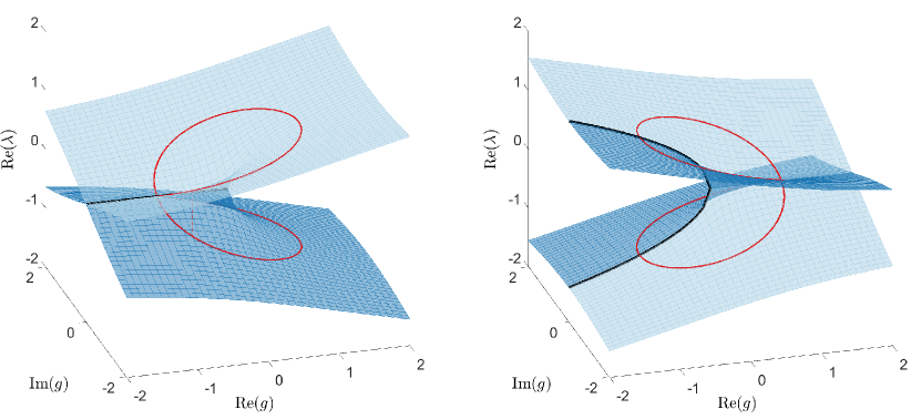
Figure 1: Plot of the real part (left) and imaginary part (right) of the multi-valued function $\lambda(g)=\pm\sqrt{g}$ (“$+$” sheet in light blue and “$-$” sheet in dark blue). The cut along the real negative semi-axis is represented as a thick black line. Each sheet is discontinuous at the cut but both of them form a single continuous surface $\lambda(g)$. The red contour depicts a full $4\pi$ turn around $g=0$ on the surface $\lambda(g)$. After a $2\pi$ turn from the point $(\lambda_{0},g_{0})$, one reaches the point $(\lambda_{0},-g_{0})$, as indicated by the red dashed line.

This basic example can be extended to other multi-valued functions. For instance, the inversion of the equation

$$F(\lambda,g)=(\lambda^{2}-1)^{2}-g=0$$ (5)

makes $\lambda(g)$ a multi-valued function with four possible values (i.e., four sheets in the complex plane):

$$\lambda_{1}(g)=\sqrt{\sqrt{g}+1}\;,\qquad\lambda_{2}(g)=\sqrt{-\sqrt{g}+1}\;,$$ (6)

$$\lambda_{3}(g)=-\sqrt{\sqrt{g}+1}\;,\qquad\lambda_{4}(g)=-\sqrt{-\sqrt{g}+1}\;.$$ (7)

This multi-valued function, shown on Fig. 2, exhibits three branch points, at which two sheets coincide: $\lambda_{1}(0)=\lambda_{2}(0)=1$, $\lambda_{3}(0)=\lambda_{4}(0)=-1$, and $\lambda_{2}(1)=\lambda_{4}(1)=0$ (note that the first two branch points occur at the same value $g=0$). Although it is visually more complicated than the square root function, it is essentially the combination of three $\sqrt{g}$-type branch points that connect four sheets together. By circling around all branch points (a contour shown in red), one goes through all sheets and reaches the initial point after a $6\pi$ turn.

Figure 2: Plot of the real part (left) and imaginary part (right) of the multi-valued function $\lambda(g)=\pm\sqrt{\pm\sqrt{g}+1}$. Four sheets are shown by different colors: $++$ in light blue, $+-$ in dark blue, $-+$ in light green and $--$ in dark green. The red contour depicts a full $6\pi$ turn around all branch points, and illustrates that all sheets are connected to each other to form a unique multi-valued surface.

In general, spectral branch points of an operator $\mathcal{B}(g)$ are related to branch points of a complex multi-valued function. From a mathematical point of view, the eigenvalues $\lambda_{1}(g),\lambda_{2}(g),\ldots$ can be interpreted as different sheets of a unique multi-valued function $\lambda(g)$ that results from the inversion of the transcendental eigenvalue equation (1). In the next subsection, we explain by computations with $2\times 2$ matrices that two crossing eigenvalues behave as $\sqrt{g-g_{0}}$ in a vicinity of their branch point.

2.2 Matrix model

Figure 3: Illustration of the transition from two real eigenvalues (left) to a complex conjugate pair (right). At $g=g_{0}$, $\lambda_{n}$ and $\lambda_{n^{\prime}}$ coincide in the complex plane. By integrating the resolvent $(\mathcal{B}(g)-\lambda\mathcal{I})^{-1}$ over a contour $\mathcal{C}_{\lambda}$, one obtains a two-dimensional projector $\Pi(g)$ that is analytical in $g$ because the resolvent is analytical outside of poles (i.e., away from the eigenvalues of $\mathcal{B}(g)$).

We illustrate the phenomenon of spectral branch points on the simplest case of a $2\times 2$ matrix (see also, e.g., [14, 59]). Although an operator ${\mathcal{B}}(g)$ acting on an infinite-dimensional vector space cannot be reduced to a matrix, the coalescence of two eigenmodes and eigenvalues is essentially captured by a computation on a vector space of dimension $2$ (note that the coalescence of a larger number of eigenmodes, that can be realized with larger matrices, leads to branch points of higher order and involves a higher-dimensional space, see [25, 26, 27] and references therein; this case is not considered here). To explain this point, we follow the suggestion by B. Helffer illustrated on Fig. 3. Let us choose an integration contour $\mathcal{C}_{\lambda}$ in the complex $\lambda$-plane that circles around two simple (non-degenerate) eigenvalues $\lambda_{n}$ and $\lambda_{n^{\prime}}$. We assume that these (and only these) eigenvalues coalesce at $g=g_{0}$. Since the spectrum is discrete, it is possible to choose the contour $\mathcal{C}_{\lambda}$ such that no other eigenvalue cross it over $|g-g_{0}|<\epsilon$ for a given small enough $\epsilon>0$. By integrating the resolvent $(\mathcal{B}(g)-\lambda\mathcal{I})^{-1}$ of the operator $\mathcal{B}(g)$ over the contour $\mathcal{C}_{\lambda}$, one obtains a two-dimensional projector $\Pi(g)$ over the space spanned by the associated eigenmodes $v_{n}$ and $v_{n^{\prime}}$, at least for $g\neq g_{0}$. Note that $\Pi(g)$ is a function of the parameter $g$ with values in the infinite-dimensional space of continuous operators over the vector space $E$. Such a resolvent expansion in the vicinity of a branch point is well known since the 1960s. For the illustrative purposes of this section, we focus on the main ideas and skip mathematical details, subtleties, and proofs that can be found in classical textbooks on operator theory (see, e.g., [3, 4]).

Since the integration contour $\mathcal{C}_{\lambda}$ does not cross any eigenvalue, the resolvent is an analytical function of $\lambda$ and $g$ over $\mathcal{C}_{\lambda}$, therefore $\Pi(g)$ is an analytical function of $g$. In particular, the image of $\Pi(g)$ is two-dimensional, even at the branch point $g=g_{0}$. As one will see, this does not imply that there are still two linearly independent eigenmodes $v_{n}$ and $v_{n^{\prime}}$ at that point. The restriction of the operator $\mathcal{B}(g)$ to the image of $\Pi(g)$ yields a $2\times 2$ matrix $\mathsf{A}(g)$. If there is no other spectral branch point over the considered range of $g$, the restriction of the operator to the kernel of $\Pi(g)$ is analytical, therefore the non-analyticity of the spectrum of $\mathcal{B}(g)$ is fully captured by the matrix $\mathsf{A}(g)$ as claimed above.

We consider a $2\times 2$ matrix of the general form

$$\mathsf{A}(g)=\left[\begin{array}[]{cc}\lambda_{0}+a&b\\ c&\lambda_{0}-a\end{array}\right]\;,$$ (8)

where $\lambda_{0},a,b,c$ are smooth functions of $g$ (the smoothness results from the analyticity of the projector $\Pi(g)$). One can easily compute its eigenvalues $\lambda_{\pm}$ and eigenvectors $\mathsf{X}_{\pm}$:

$$\lambda_{\pm}=\lambda_{0}\pm\sqrt{d}\;,\qquad\mathsf{X}_{\pm}=\left[\begin{array}[]{c}b\\ \pm\sqrt{d}-a\end{array}\right]\;,$$ (11)

where $d=bc+a^{2}$. If $d\neq 0$, the eigenvalues are distinct while the associated eigenvectors are linearly independent. In turn, if $d(g_{0})=0$ at some point $g_{0}$, the eigenvalues coincide at $g=g_{0}$. We first consider a Hermitian matrix and then we show how the general non-Hermitian case differs qualitatively.

(i) If $\mathsf{A}(g)$ is Hermitian for all values of $g$, then $a\in\mathbb{R}$ and $c=b^{*}$, so that $d=|b|^{2}+a^{2}$ is real and non-negative. Furthermore, the condition $d(g_{0})=0$ implies $a(g_{0})=b(g_{0})=c(g_{0})=0$. This also yields $d^{\prime}(g_{0})=0$, while $d^{\prime\prime}(g_{0})\neq 0$ in general, so that the eigenvalues in a vicinity of $g_{0}$ are approximately equal to

$$\lambda_{\pm}\approx\lambda_{0}(g_{0})\pm\sqrt{d^{\prime\prime}(g_{0})/2}\,(g-g_{0})\;.$$ (12)

Thus one can draw two main conclusions: (i) the spectrum does not present non-analytical branch points, the eigenvalues merely cross each other at $g=g_{0}$; (ii) the dimension of the eigenspace $E_{\lambda_{0}}$ at $g=g_{0}$ is $2$. Such a coalescence point is called diabolic point [60, 15, 16, 61].

(ii) Now we turn to the non-Hermitian case. The function $d(g)$ takes complex values and crosses $0$ at $g=g_{0}$ with a non-zero derivative $d^{\prime}(g_{0})$. The phases of $\lambda_{\pm}-\lambda_{0}$ undergo a $\pi/2$ jump when $g$ passes through the critical value $g_{0}$ and the absolute value of $\lambda_{\pm}-\lambda_{0}$ behaves typically as $\sqrt{d^{\prime}(g_{0})(g-g_{0})}$ for $g$ close to $g_{0}$. In particular, if $d(g)$ is real (positive for $g<g_{0}$ and negative for $g>g_{0}$), and if $\lambda_{0}(g_{0})$ is real, one obtains in a vicinity of the critical value $g_{0}$:

$$g<g_{0}\qquad \left\{\begin{array}[]{l}\mathrm{Re}(\lambda_{\pm})\approx\lambda_{0}(g_{0})\pm\sqrt{d^{\prime}(g_{0})(g_{0}-g)}\\ \mathrm{Im}(\lambda_{\pm})=0\end{array}\right.\vspace{6pt}$$ (15)

$$g>g_{0}\qquad \left\{\begin{array}[]{l}\mathrm{Re}(\lambda_{\pm})=\lambda_{0}(g_{0})\\ \mathrm{Im}(\lambda_{\pm})\approx\pm\sqrt{d^{\prime}(g_{0})(g-g_{0})}\end{array}\right.$$ (18)

At the critical value $g=g_{0}$, the matrix $\mathsf{A}(g_{0})$ is in general not diagonalizable. Without loss of generality, let us assume that $b(g_{0})\neq 0$. The matrix $\mathsf{A}(g_{0})$ can then be reduced to a Jordan block with an eigenvector $\mathsf{X}_{0}$ and a generalized eigenvector $\mathsf{Y}_{0}$:

$$\mathsf{A}(g_{0})\mathsf{X}_{0}=\lambda_{0}\mathsf{X}_{0}\;,\qquad\mathsf{X}_{0}=\left[\begin{array}[]{c}b(g_{0})\\ -a(g_{0})\end{array}\right]\;,$$ (21)

$$\mathsf{A}(g_{0})\mathsf{Y}_{0}=\lambda_{0}\mathsf{Y}_{0}+\mathsf{X}_{0}\;,\qquad\mathsf{Y}_{0}=\left[\begin{array}[]{c}0\\ 1\end{array}\right]\;.$$ (24)

Note that since the derivative of $\sqrt{d(g)}$ is infinite at $g=g_{0}$, one has

$$\mathsf{Y}_{0}={\left.\kern-1.2pt\frac{d\mathsf{X}_{\pm}}{d\lambda_{\pm}}\right|_{g=g_{0}}}\;,$$ (25)

where the derivative yields the same result for $(\mathsf{X}_{+},\lambda_{+})$ and $(\mathsf{X}_{-},\lambda_{-})$. Moreover, if $\mathsf{A}(g)$ is a symmetric matrix (i.e. $b=c$), then $\mathsf{X}_{0}^{T}\mathsf{X}_{0}=a^{2}(g_{0})+b^{2}(g_{0})=d(g_{0})=0$, i.e., $\mathsf{X}_{0}$ is “orthogonal” to itself for the real scalar product.

In comparison to the Hermitian case, there are two main conclusions: (i) the spectrum is non-analytical at $g=g_{0}$; (ii) the eigenvectors $\mathsf{X}_{\pm}$ of $\mathsf{A}(g)$ collapse onto a single eigenvector $\mathsf{X}_{0}$ as $g\to g_{0}$, and the matrix $\mathsf{A}(g_{0})$ can be reduced to a Jordan block with a generalized eigenvector $\mathsf{Y}_{0}$ given by the rate of change of the eigenvectors $\mathsf{X}_{\pm}$ with their corresponding eigenvalues $\lambda_{\pm}$, evaluated at the critical point $g=g_{0}$. Such a coalescence point is called exceptional point.

We summarize the results for the Hermitian and non-Hermitian cases graphically on Fig. 4. We emphasize that the dichotomy “Hermitian $\leftrightarrow$ no branching” versus “non-Hermitian $\leftrightarrow$ branching” is specific to two-dimensional matrices. For instance, if one considers a $4\times 4$ matrix made of two $2\times 2$ blocks where one is Hermitian and the other is non-Hermitian, then the eigenvalues of the Hermitian block do not exhibit any branch point when they cross, even if the whole matrix is not Hermitian. This somewhat artificial example shows that there is no general relation between branch points and the non-Hermitian property, except that the spectrum of a Hermitian operator never branches. By reducing the full operator to a low-dimensionality matrix on the subspace associated to the crossing point, one can make precise statements about branching and Hermitian character, as we did in this two-dimensional case. The “translation” of the above conclusions to the case of the Bloch-Torrey operator and their consequences on spectral decompositions are detailed in Sec. 3.3.

 

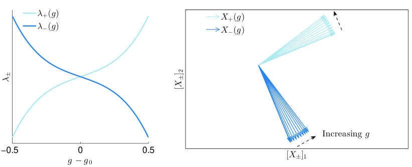
Figure 4: Eigenvalues and eigenvectors of a general $2\times 2$ matrix $\mathsf{A}(g)$. (Top) Hermitian case: the eigenvalues $\lambda_{\pm}(g)$ cross each other at $g=g_{0}$, the eigenvectors $X_{\pm}(g)$ are always orthogonal to each other and do not exhibit any particular behavior at $g=g_{0}$. (Bottom) non-Hermitian case: the eigenvalues $\lambda_{\pm}(g)$ exhibit a typical square-root behavior near $g=g_{0}$ (indicated by a red cross), the eigenvectors $X_{\pm}(g)$ collapse onto a single vector at $g=g_{0}$ (indicated by a red arrow). Note that $g$ was sampled with additional points near $g_{0}$ for a better visualization of the branching. The complex $X_{\pm}$ vectors were plotted with the convention that $\mathrm{arg}([X_{\pm}]_{1})=0$.

3 The Bloch-Torrey operator

In this section we apply the previous considerations to the Bloch-Torrey operator which governs the time evolution of the transverse magnetization $m(t,\mathbf{r})$ in diffusion NMR experiments [39, 40, 41, 42, 43, 44, 45, 46]. For a given Euclidean domain $\Omega\subset{\mathbb{R}}^{d}$ ($d\geq 1$) with a smooth enough boundary $\partial\Omega$, the transverse magnetization of the spin-bearing particles obeys the Bloch-Torrey equation [38]

$$\partial_{t}\,m(t,\mathbf{r})=D\nabla^{2}m(t,\mathbf{r})+i\gamma Gx\,m(t,\mathbf{r}),$$ (26)

subject to some initial magnetization $m(0,\mathbf{r})$ and to Neumann boundary condition:

$${\left.\kern-1.2pt\mathbf{n}\cdot\nabla m\right|_{\partial\Omega}}=0\;,$$ (27)

where $\mathbf{n}$ is the inward normal vector at the boundary, $D$ is the diffusion coefficient, $\gamma$ is the gyromagnetic ratio, and $G$ is the amplitude of the magnetic field gradient applied along some spatial direction $x$ (here the gradient is considered to be time-independent). The Laplace operator $\nabla^{2}$ governs diffusion of the spin-bearing particles while the imaginary “potential” $-i\gamma Gx$ describes the magnetization precession in the transverse plane due to the applied magnetic field gradient. Denoting $g=\gamma G/D$, the solution of this equation can be formally written as $m(t,\mathbf{r})=e^{-\mathcal{B}(g)Dt}m(0,\mathbf{r})$, where we introduced the Bloch-Torrey operator

$$\mathcal{B}(g)=-\nabla^{2}-igx$$ (28)

that acts on functions on the domain $\Omega$, subject to the boundary condition (27) (for a rigorous mathematical definition, see e.g. [53, 54, 55]). Even though the parameter $g$ is real in the context of diffusion NMR, we consider the general case $g\in{\mathbb{C}}$.

In the one-dimensional setting, $\mathcal{B}(g)$ is more commonly known as the (complex) Airy operator [4, 51]. For a half-line $\Omega=\mathbb{R}_{+}$, its eigenmodes are known explicitly in terms of the Airy function, whereas the eigenvalues are expressed in terms of its zeros [47, 50, 51] (see also [62, 63] for relations to higher-order polynomial potentials). This is the only known example, for which the spectrum of the Bloch-Torrey operator is fully explicit. Even for an interval, $\Omega=(a,b)$, one has to solve numerically a transcendental equation to determine the eigenvalues (see [47, 50] for details). Despite this difficulty, Stoller et al. managed to discover and accurately characterize branch points in the spectrum [47].

In higher dimensions ($d\geq 2$), a linear combination of the Laplace operator $-\nabla^{2}$ and a coordinate-linear potential term $-igx$ along a single spatial direction naturally suggests a spatial splitting of the setup into this (longitudinal) direction and its orthogonal (transversal) coordinate hyperplane. One can therefore represent the Bloch-Torrey operator as a sum of the corresponding one-dimensional Airy-type operator and the Laplace operator in the transversal hyperplane. The mode coupling (and mixing) occurs through the boundary conditions (27). The spectral properties of the Bloch-Torrey operator have been studied in different geometric settings, including bounded, unbounded and periodic domains [48, 49, 50, 51, 52, 53, 54, 55, 56, 57]. For instance, the asymptotic behavior of the eigenvalues and eigenfunctions in the semi-classical limit $g\to\infty$ has been analyzed. In turn, the existence of branch points in the spectrum of the Bloch-Torrey operator in Euclidean domains with $d\geq 2$ remains unknown, except for a numerical example given in [56].

Throughout this section we assume that the domain $\Omega$ is bounded. Under this assumption, the gradient term is a bounded perturbation of the Laplace operator that ensures the existence of a discrete set of eigenpairs (eigenmode and eigenvalue) $(v_{n},\lambda_{n})$, indexed by $n=1,2,\ldots$ and ordered according to the growing real part of $\lambda_{n}$. If $g$ is not a branch point (see below), the eigenmodes are orthonormal, $(v_{n}|v_{k})=\delta_{n,k}$, with respect to the bilinear form

$$(f|g)=\int_{\Omega}f(\mathbf{r})g(\mathbf{r})\,d\mathbf{r}\;.$$ (29)

We recall that there is no complex conjugate in the definition of $(\cdot|\cdot)$ because the Bloch-Torrey operator is not Hermitian. This normalization implies that each eigenmode is defined up to a sign (in contrast to Hermitian operators, there is no arbitrary phase factor $e^{i\alpha}$).

We first show how spectral branch points appear for real values of $g$ in parity symmetric domains. Interestingly, this branching phenomenon is associated to a dramatic change in the behavior of the eigenmodes of the Bloch-Torrey operator, with an abrupt transition from delocalized to localized states (see below). Then we turn to general domains and present a simple numerical algorithm to detect branch points in the complex $g$-plane.

3.1 Parity-symmetric domains

Let us assume that the domain $\Omega$ is invariant by an isometric transformation that reverses the $x$-axis (i.e., $\pi$ rotation around an axis orthogonal to $\mathbf{e_{x}}$ or mirror symmetry with respect to the plane orthogonal to $\mathbf{e_{x}}$), see Fig. 5. We call this transformation $x$-parity in short and denote it by $\mathcal{P}_{x}$. Under the combination $x$-parity and complex conjugation, the Bloch-Torrey operator becomes

$$\mathcal{P}_{x}\mathcal{B}(g)^{*}=(-\nabla^{2}-ig(-x))^{*}=\mathcal{B}(g^{*})\;.$$ (30)

In this subsection, we focus on the case of real $g$ so that the Bloch-Torrey operator is invariant under $x$-parity plus complex conjugation (since the complex conjugation is associted with time reversal in quantum mechanics, one usually speaks about ${\mathcal{P}}{\mathcal{T}}$ symmetry). Therefore, if $v_{n}$ is an eigenmode with an eigenvalue $\lambda_{n}$, then $\mathcal{P}_{x}v_{n}^{*}$ is an eigenmode with the eigenvalue $\lambda_{n}^{*}$. This leads to two possible situations.

Figure 5: Illustration of two domains that are symmetric under $x$-parity: (left) the domain is symmetric under mirror symmetry indicated by red dotted line; (right) the domain is symmetric under central symmetry indicated by red cross.

1. the eigenvalue $\lambda_{n}$ is real (and simple), so that $v_{n}=\pm\mathcal{P}_{x}v_{n}^{*}$. In this case, the eigenmode $v_{n}$ is “symmetric” in the sense that $|v_{n}|$ is invariant by $x$-parity. Note that this is consistent with the previous paragraph: the imaginary part of $\lambda_{n}$ is zero and the eigenmode is centered around $x=0$. We call such an eigenmode “delocalized” as it spreads over the whole domain.

2. two eigenvalues $\lambda_{n}$ and $\lambda_{n^{\prime}}$ form a complex conjugate pair, so that $v_{n^{\prime}}=\pm\mathcal{P}_{x}v_{n}^{*}$. This means that the eigenmode $v_{n^{\prime}}$ is an $x$-parity “reflection” of $v_{n}$. We call such an eigenmode “localized” as it is mainly concentrated on one side of the domain and is almost zero on the other side.

The transition from case (i) to case (ii), i.e. from two real eigenvalues $\lambda_{n}$ and $\lambda_{n^{\prime}}$ to a complex conjugate pair may occur only if $\lambda_{n}$ and $\lambda_{n^{\prime}}$ coincide at some value $g_{0}$. As illustrated on Fig. 3, the coalescence of two eigenvalues results in a branch point in the spectrum, i.e., a non-analyticity. Such branch points mark the transition from delocalized eigenmodes (i) to localized eigenmodes (ii) that are at the origin of the localization regime. This phenomenon was first discovered by Stoller et al. for the Bloch-Torrey operator in an interval with Neumann boundary condition [47].

Figure 6 illustrates their discovery and the above discussion for the unit interval $(-1/2,1/2)$. On the top, the real and imaginary parts of the first two eigenvalues $\lambda_{1}(g)$ and $\lambda_{2}(g)$ are shown as functions of $g$ (this figure can be considered as a zoom of the rescaled figure 3 from [47]). At $g=0$, one retrieves the eigenvalues of the second derivative operator ${\mathcal{B}}(0)=-d^{2}/dx^{2}$: $\lambda_{n}(0)=\pi^{2}(n-1)^{2}$, with $n=1,2,3,\ldots$. A transition from two real eigenvalues to a complex conjugate pair occurs at the branch point $g_{c}\approx 18.1$, in perfect agreement with the theoretical prediction by Stoller et al. (see also Sec. 4). This qualitative change of the eigenvalues is also reflected in the behavior of the associated eigenmodes $v_{1}(x)$ and $v_{2}(x)$, whose real and imaginary parts are shown on the middle and bottom panels of Fig. 6. Here we plot $51$ eigenmodes for $51$ equally spaced values of $g$ ranging from $0$ to $100$. At $g=0$, one retrieves the eigenmodes of the second derivative with Neumann boundary conditions at $x=\pm 1/2$, namely $v_{1}(x)=1$ and $v_{2}(x)=\sqrt{2}\sin(\pi x)$. As $g$ increases up to $g_{c}$, the shape of these eigenmodes continuously changes but they remain to be qualitatively similar and “delocalized”. In particular, the real parts of $v_{1}(x)$ and $v_{2}(x)$ are respectively symmetric and antisymmetric with respect to the middle point of the interval. However, at the branch point, there is a drastic change in the behavior of these eigenmodes. As two eigenmodes coalesce into a single one, their normalization factors $(v_{1}|v_{1})^{2}$ and $(v_{2}|v_{2})^{2}$ vanish (see below), implying a considerable increase of the amplitudes of $v_{1}$ and $v_{2}$ for $g$ near $g_{0}$ (see thick blue curves). For $g>g_{c}$, the parity symmetry of these eigenmodes implies $\mathrm{Re}(v_{2}(x))=\mathrm{Re}(v_{1}(1-x))$ and $\mathrm{Im}(v_{2}(x))=-\mathrm{Im}(v_{1}(1-x))$. As $g$ increases, the eigenmode $v_{1}(x)$ progressively shifts to the right endpoint $x=1$, near which it is getting more and more localized (i.e., its amplitude on the left half of the interval is reduced). Likewise, the eigenmode $v_{2}(x)$ is getting localized near the left endpoint $x=0$. Such an abrupt change in the shape and symmetries of the eigenmodes at the branch point is a remarkable feature of non-Hermitian operators.

The above argument also implies that if the branch point $g_{0}$ with the smallest amplitude $|g_{0}|$ lies on the real axis, all eigenvalues $\lambda_{n}(g)$ of the Bloch-Torrey operator are necessarily real for any $0<g<|g_{0}|$. This is an example of a non-Hermitian operator with a real spectrum. Actually, there are many families of such operators [64, 65, 66, 67, 68, 69, 70, 71] (see also a review [72]).

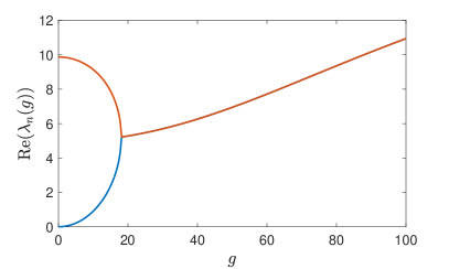
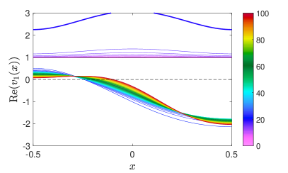
Figure 6: The spectrum of the Bloch-Torrey operator on the interval $(-1/2,1/2)$ with Neumann boundary conditions. (Top) The real (left) and imaginary (right) part of the first two eigenvalues $\lambda_{1}(g)$ and $\lambda_{2}(g)$ as functions of $g$. A transition from of two real eigenvalues to a complex conjugate pair occurs at the branch point $g_{c}\approx 18.06$. (Middle, Bottom) The real (left) and imaginary (right) part of the first eigenmode $v_{1}(x)$ (middle) and of the second eigenmode $v_{2}(x)$ (bottom). $51$ plotted curves correspond to $51$ equally spaced values of $g$ from $0$ to $100$ (shown by colorbar). Black line depicts the Laplacian eigenmodes ($g=0$), whereas thick blue line shows the eigenmodes at $g=18$ (near the branch point $g_{c}\approx 18.06$).

3.2 Arbitrary bounded domains

For a parity-symmetric domain, the spectrum exhibits branch points at particular values of the gradient $g\in{\mathbb{R}}$. In contrast, for a general domain without parity symmetry, all eigenvalues are generally complex for non-zero $g$ and there is generally no branch point on the real line. However, this is true only for real values of $g$. By allowing $g$ to take complex values, one may recover branch points for general bounded domains. In other words, an asymmetry of the domain typically “shifts” branch points away from the real axis.

The point of view onto spectral branch points as complex branch points of a multi-valued function reveals a way to find them in the complex plane. Let us consider a closed contour $\mathcal{C}_{g}$ in the complex $g$-plane and compute the contour integral

$$I_{n}(\mathcal{C}_{g})=\oint_{\mathcal{C}_{g}}\lambda_{n}(g)\,\mathrm{d}g\;.$$ (31)

If $\mathcal{C}_{g}$ does not enclose any branch point, then $\lambda_{n}(g)$ is analytical inside the contour for any sheet $n=1,2,\ldots$, and one has $I_{n}(\mathcal{C}_{g})=0$. In contrast, if the contour $\mathcal{C}_{g}$ encloses branch points, the contour integral along $\mathcal{C}_{g}$ is generally non zero anymore. Therefore, one can find branch points by the following algorithm:

1. choose an initial closed contour $\mathcal{C}_{g}$ and compute $I_{n}(\mathcal{C}_{g})$ with $n=1,2,\ldots,N$ for a large enough number $N$ of sheets by following continuously the contour $\mathcal{C}_{g}$;

2. if the obtained value is not zero, split the contour in smaller closed contours and perform the integral over each smaller contour;

3. identify contours with non-zero integrals and repeat the previous step for each of them.

In this way, one can determine a finite number of branch points inside the initial contour. However, additional restrictions on the spectral properties are needed to ensure that all branch points inside the contour are identified. For instance, branch points should not accumulate near a point inside the contour. Figure 7 illustrates an application of this algorithm for the Bloch-Torrey operator on a symmetric domain (a disk) and an asymmetric domain (an oval).

 

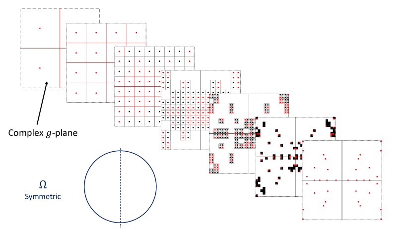
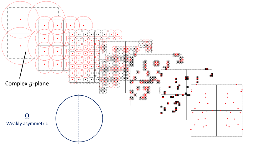
Figure 7: Several iterations of the algorithm that finds spectral branch points of the Bloch-Torrey operator in the complex $g$-plane. The red dots indicate contours that yield a non-zero contour integral. The initial range of $g$ is a square in the complex plane, from $-200(1+i)$ to $200(1+i)$. We emphasize that there are infinitely many branch points in the complex plane but only a finite number appears because of the finite range of $g$. (Top) The domain $\Omega$ is a disk and we apply the algorithm with square integration contours. (Bottom) The domain $\Omega$ is slightly asymmetric (a thin dashed line helps to visualize the asymmetry) and we apply the algorithm with circular integration contours. Compared to the pattern of branch points for a disk, the top-bottom symmetry is lost but branch points still exist. Note that the left-right symmetry is preserved in both plots, as discussed in the text.

In practice, each integral is computed numerically by discretizing its contour $\mathcal{C}_{g}$, i.e., $I_{n}(\mathcal{C}_{g})\approx I_{n}^{\rm num}(\mathcal{C}_{g})$. As a consequence, the numerically computed integral is never equal to $0$, even if there is no branch point inside the contour. One needs therefore to choose a numerical threshold $\chi$ to distinguish between “zero” and “non-zero” integrals (indicated in Fig. 7 by black and red dots, respectively). A compromise should be found between reliability and speed of the algorithm. In fact, a too high threshold may result in missed branch points: if $0<|I_{n}(\mathcal{C}_{g})|<\chi$, such branch point(s) inside the contour $\mathcal{C}_{g}$ are not detected. In turn, a too small threshold generally leads to a large number of evaluations of contour integrals: even if there is no branch point inside $\mathcal{C}_{g}$ (and thus $I_{n}(\mathcal{C}_{g})=0$), numerical errors may result in $|I_{n}^{\rm num}(\mathcal{C}_{g})|>\chi$, so that the algorithm continues subdivisions into smaller contours until all the contour integrals become less than $\chi$. Since each integral requires the computation of the eigenvalues $\lambda_{n}(g)$ along the contour $\mathcal{C}_{g}$, a bad choice of the threshold may be very time-consuming (see A for the spectrum computation in the case of the Bloch-Torrey operator). For the particular example shown on Fig. 7, one can see that the threshold was chosen somewhat too low because some red squares at the initial steps eventually disappeared after a large number of iterations. In other words, a suspicion of missed branch points was dismissed but it required an excessive number of computations.

The choice of the contour is also a matter of compromise. On one hand, one can choose a contour shape that tiles the plane, like a square. This choice allows one to have non-overlapping integration contours to avoid counting one branch point twice. On the other hand, one can choose a smooth contour, like a circle. This results in a higher numerical accuracy for the integral computation and thus allows one to lower the threshold. However, this requires an additional criterion to discard “double” branch points that may result from overlapping contours. Both options are illustrated on Fig. 7.

Figure 8: Real (top) and imaginary (bottom) part of the spectrum of the Bloch-Torrey operator in a disk (see also top panel of Fig. 7). Several sheets are shown by different colors. The figure reveals a rich pattern of branch points, with a similar structure as in Figs. 1 and 2.

Let us inspect the pattern of branch points shown on Fig. 7. Performing a complex conjugation of the Bloch-Torrey operator,

$$\mathcal{B}(g)^{*}=-\nabla^{2}+ig^{*}x=-\nabla^{2}-i(-g^{*})x\;,$$ (32)

we see that the branch points are always symmetric under the transformation $g\to-g^{*}$, that explains the left-right symmetry of their pattern. Furthermore, the pattern for $x$-parity-symmetric domains (like a disk) exhibits a top-bottom symmetry, according to

$$\mathcal{P}_{x}\mathcal{B}(g)^{*}=-\nabla^{2}-ig^{*}x\;,$$ (33)

where we used the parity symmetry to write $\mathcal{P}_{x}\nabla^{2}=\nabla^{2}$. The above equation shows that for an $x$-parity symmetric domain, the pattern of branch points is symmetric under the transformation $g\to g^{*}$, i.e. the top-bottom symmetry. Note that the existence of branch points on the real axis is consistent with the top-bottom symmetry of their pattern.

To get a complementary insight, Fig. 8 shows several sheets of the multi-valued function $\lambda(g)$ for the Bloch-Torrey operator in a disk. Although the figure is visually complicated due to the superposition of numerous sheets, one can recognize the basic square-root structure of branch points illustrated on Fig. 1.

3.3 Spectral decomposition at a branch point

Let us “translate” the general statements of Sec. 2.2 about the second-order branch points analyzed with a matrix model, into the language of eigenmodes of the Bloch-Torrey operator. In particular, we investigate the validity of the spectral decomposition

$$f(\mathbf{r})\binrel@{=}\binrel@@{\mathop{\kern 0.0pt=}\limits^{?}}\sum_{n}{(f|v_{n})}v_{n}(\mathbf{r})\;,$$ (34)

where the bilinear form $(\cdot|\cdot)$ is defined in Eq. (29). As the eigenbasis formed by $v_{n}$ is not necessarily complete, the validity of Eq. (34), which was often used in physics literature, is not granted. As the arguments and techniques employed below are rather standard, we focus on qualitative explanations while mathematical details can be found, e.g., in [58, 15, 16, 61, 59].

3.3.1 Behavior of the eigenmodes at a branch point.

Let us consider two eigenpairs $(v_{1},\lambda_{1})$ and $(v_{2},\lambda_{2})$ that undergo branching at $g=g_{0}$. The matrix model of Sec. 2.2 shows that $v_{1}$ and $v_{2}$ collapse onto a single eigenmode $v_{0}$ at the branch point. Moreover, since $v_{1}$ and $v_{2}$ are “orthogonal” with respect to the bilinear form $(\cdot|\cdot)$ if $g\neq g_{0}$, we conclude by continuity that $v_{0}$ is self-orthogonal, i.e. $(v_{0}|v_{0})=0$. We outline that the condition $(v_{0}|v_{0})=0$ may be achieved for a nonzero complex-valued function $v_{0}$ because $(\cdot|\cdot)$ does not contain complex conjugate, see Eq. (29).

The computations in Sec. 2.2 imply the following behavior in a vicinity of the branch point $g_{0}$:

$$v_{1}(\mathbf{r})\approx\beta_{1}(g)\left[v_{0}(\mathbf{r})+(g-g_{0})^{1/2}y_{0}(\mathbf{r})\right]\;,$$ (35)

$$v_{2}(\mathbf{r})\approx\beta_{2}(g)\left[v_{0}(\mathbf{r})-(g-g_{0})^{1/2}y_{0}(\mathbf{r})\right]\;,$$ (36)

where $\beta_{1}(g)$ and $\beta_{2}(g)$ are normalization constants, and the function $y_{0}(\mathbf{r})$ is a priori unknown and depends on the details of the branch point under study. The form (3.3.1) ensures that $v_{1}$ and $v_{2}$ are orthogonal to each other to the first order in $(g-g_{0})^{1/2}$, i.e., $(v_{1}|v_{2})=O(g-g_{0})$. Moreover, the normalization conditions imply

$$1 =(v_{1}|v_{1})\approx 2\beta_{1}^{2}(g)(g-g_{0})^{1/2}(v_{0}|y_{0}),$$ (37)

$$1 =(v_{2}|v_{2})\approx-2\beta_{2}^{2}(g)(g-g_{0})^{1/2}(v_{0}|y_{0}),$$ (38)

therefore

$$v_{1}(\mathbf{r})\approx C(g-g_{0})^{-1/4}v_{0}(\mathbf{r})+C(g-g_{0})^{1/4}y_{0}(\mathbf{r})\;,$$ (39)

$$v_{2}(\mathbf{r})\approx iC(g-g_{0})^{-1/4}v_{0}(\mathbf{r})-iC(g-g_{0})^{1/4}y_{0}(\mathbf{r})\;,$$ (40)

with the constant $C=(2(v_{0}|y_{0}))^{-1/2}$. We recall that the eigenvalues $\lambda_{1}$ and $\lambda_{2}$ behave near $g_{0}$ as

$$\lambda_{1}\approx\lambda_{0}(g_{0})+(g-g_{0})^{1/2}\eta_{0}\;,\qquad\lambda_{1}\approx\lambda_{0}(g_{0})-(g-g_{0})^{1/2}\eta_{0}\;,$$ (41)

with an unknown coefficient $\eta_{0}$. By writing the Bloch-Torrey operator as

$$\mathcal{B}=\mathcal{B}_{0}-i(g-g_{0})x\;,\qquad\mathrm{with}\quad\mathcal{B}_{0}=-\nabla^{2}-ig_{0}x,$$ (42)

one can expand the eigenmode equation $\mathcal{B}v_{1}=\lambda_{1}v_{1}$ in powers of $(g-g_{0})$ and get in the lowest order

$$\mathcal{B}_{0}y_{0}=\lambda_{0}y_{0}+\eta_{0}v_{0}\;.$$ (43)

One recognizes in this equation the typical Jordan block associated to a branch point (see Sec. 2.2).

3.3.2 Regularity of the spectral decomposition at a branch point.

The above equations (3.3.1) reveal that the eigenmodes $v_{1}$ and $v_{2}$ diverge as $(g-g_{0})^{-1/4}$ at the branch point. This behavior is intuitively expected because $v_{1}$ and $v_{2}$ tend to the self-orthogonal eigenmode $v_{0}$, therefore the normalization constants $\beta_{1}$ and $\beta_{2}$ should diverge as $g\to g_{0}$. One may wonder whether this divergence produces specific effects in the spectral decomposition (34) such as a resonance effect when two eigenmodes near a branch point could dominate the series. We show here that this is not the case because two infinitely large contributions in Eq. (3.3.1) cancel each other, yielding a continuous behavior in the limit $g\to g_{0}$. Note that this regularization follows from the general argument that the projector $\Pi(g)$ over the space spanned by $v_{1}$ and $v_{2}$ is an analytical function of $g$ at the branch point (see Sec. 2.2).

Let us isolate the terms with $v_{1}$ and $v_{2}$ in the sum (34) and define

$$f_{1,2}(\mathbf{r})=(f|v_{1})v_{1}(\mathbf{r})+(f|v_{2})v_{2}(\mathbf{r})\;.$$ (44)

Now we use the expansions (3.3.1) to obtain, in a vicinity of the branch point:

$$f_{1,2}(\mathbf{r}) \approx C^{2}\biggl{(}(g-g_{0})^{-1/4}(f|v_{0})+(g-g_{0})^{1/4}(f|y_{0})\biggr{)}$$ (45)

$$\times\biggl{(}(g-g_{0})^{-1/4}v_{0}(\mathbf{r})+(g-g_{0})^{1/4}y_{0}(\mathbf{r})\biggr{)}$$

$$-C^{2}\biggl{(}(g-g_{0})^{-1/4}(f|v_{0})-(g-g_{0})^{1/4}(f|y_{0})\biggr{)}$$

$$\times\biggl{(}(g-g_{0})^{-1/4}v_{0}(\mathbf{r})-(g-g_{0})^{1/4}y_{0}(\mathbf{r})\biggr{)},$$

which simplifies to

$$f_{1,2}(\mathbf{r})\approx\frac{(f|y_{0})}{(v_{0}|y_{0})}v_{0}(\mathbf{r})+\frac{(f|v_{0})}{(v_{0}|y_{0})}y_{0}(\mathbf{r})+O((g-g_{0})^{1/2})\;.$$ (46)

Two important observations can be made: (i) the diverging terms $(g-g_{0})^{-1/4}$ have canceled each other so that $f_{1,2}(\mathbf{r})$ has a finite value in the limit $g\to g_{0}$; (ii) at the branch point, $f_{1,2}(\mathbf{r})$ is expressed as a linear combination of the eigenmode $v_{0}(\mathbf{r})$ and the additional function $y_{0}(\mathbf{r})$. This shows that the spectral decomposition is still valid if the eigenmode family is supplemented with a “generalized eigenmode” $y_{0}(\mathbf{r})$. Note that the function $y_{0}(\mathbf{r})$ is the analogous of the vector $Y_{0}$ for the matrix model considered in Sec. 2.2.

If the function $f$ represents the magnetization, then one can compute its time evolution by exponentiating the Bloch-Torrey operator ${\mathcal{B}}(g_{0})$ over the basis $(v_{0},y_{0},v_{3},v_{4},\ldots)$. The only difference with the general case $g\neq g_{0}$ lies in the $2\times 2$ Jordan block associated to the pair $v_{0},y_{0}$ (see Eq. (43)) that yields

$$\exp\left(-t\left[\begin{array}[]{cc}\lambda_{0}&\eta_{0}\\ 0&\lambda_{0}\end{array}\right]\right)=\exp(-\lambda_{0}t)\left[\begin{array}[]{cc}1&-\eta_{0}t\\ 0&1\end{array}\right]\;.$$ (47)

One may recognize the typical $te^{-t}$ evolution of a critically damped harmonic oscillator, which also originates from the exponential of a Jordan block. Therefore, the evolution of the magnetization during an extended gradient pulse at $g_{0}$ is given by

$$m(t,\mathbf{r})=\frac{(1|y_{0})-\eta_{0}t(1|v_{0})}{(v_{0}|y_{0})}v_{0}(\mathbf{r})e^{-\lambda_{0}t}+\frac{(1|v_{0})}{(v_{0}|y_{0})}y_{0}(\mathbf{r})e^{-\lambda_{0}t}+\sum_{n\geq 3}(1|v_{n})v_{n}(\mathbf{r})e^{-\lambda_{n}t}\;.$$ (48)

In summary, the spectral expansion (34) is valid for any $g$ except for a set $\mathcal{E}$ of branch points. In turn, when $g=g_{0}\in\mathcal{E}$, the two eigenmodes $v_{n}$ and $v_{n^{\prime}}$ that correspond to equal eigenvalues $\lambda_{n}(g_{0})=\lambda_{n^{\prime}}(g_{0})$, merge into a single eigenmode $v_{0}$ that should thus be supplemented by a generalized eigenmode $y_{0}$. A rigorous demonstration of this conclusion and its further developments present an interesting perspective.

3.4 Summary

Figure 9 summarizes our findings by showing several eigenvalues and the corresponding eigenmodes of the Bloch-Torrey operator in a disk of diameter $L$, as a function of the dimensionless quantity $Lg^{1/3}$. The power $1/3$ has no particular significance but was chosen to improve the clarity of the figure. At $g=0$, the Bloch-Torrey operator is reduced to the Laplace operator with the well-known eigenmodes [73]. The rotational invariance of the disk implies that some eigenvalues are twice degenerate, in which case one eigenmode can be transformed to its “twin” by an appropriate rotation. When $g>0$ is small enough, the symmetries of the eigenmodes are preserved and can be distinguished by signs $(\pm,\pm)$, where the first sign refers to the symmetry along the $x$-axis ($+$ for symmetric and $-$ for antisymmetric), and the second sign refers to the symmetry along the $y$-axis. The symmetry of the Laplacian eigenmodes is of considerable importance because the gradient term $igx$ couples only the modes with the same symmetry along $y$ and with the opposite symmetries along $x$. In other words, the gradient couples $(+,+)$ to $(-,+)$ and $(-,-)$ to $(+,-)$. For example, the first branch point (blue curves) involves the constant eigenmode with symmetry $(+,+)$, and the eigenmode with symmetry $(-,+)$ immediately above. A more complicated branching pattern can be observed with the light orange curve, which has a $(+,+)$ symmetry. One can see that it goes up and branches with the dark orange curve that corresponds to the $(-,+)$ eigenmode at the top of the figure. However, a careful examination reveals that this eigenmode branches first with the $(+,+)$ eigenmode right below it, then they split again before branching with the light orange curve.

At a large gradient strength, nearly all plotted eigenvalues have branched, and the associated eigenmodes are localized on one side of the domain. Consistently with our results, eigenvalues with positive imaginary part correspond to eigenmodes localized on the left side of the disk. By applying the theory of localization at a curved boundary [74, 48], one can assign to each eigenmode two indices $(n,l)$ that describe the behavior of the eigenmode in the directions perpendicular and parallel to the boundary. As the order $n$ increases, the extension of the eigenmodes along $x$ increases until a point where they cannot be localized anymore. This explains why the branch points associated to larger values of $n$ occur at larger values of $g$.

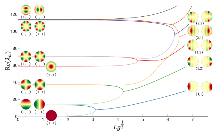
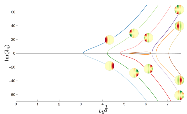
Figure 9: Spectral properties of the Bloch-Torrey operator in a disk of diameter $L=1$. Real (top) and imaginary (bottom) parts of several eigenvalues $\lambda_{n}(g)$ as functions of $Lg^{1/3}$. At $g=0$, one retrieves the eigenvalues of the Laplace operator with Neumann boundary condition: $\lambda_{1}(0)=0$, $\lambda_{2}(0)=\lambda_{3}(0)=4(j^{\prime}_{1,1})^{2}\approx 13.56$, $\lambda_{4}(0)=\lambda_{5}(0)=4(j^{\prime}_{2,1})^{2}\approx 37.31$, $\lambda_{6}(0)=4(j^{\prime}_{0,2})^{2}\approx 58.68$, etc., where $j^{\prime}_{n,k}$ denotes the $k$-th zero of $J^{\prime}_{n}(z)$ [73]. The symmetries of the corresponding eigenmodes are distinguished by two signs $(\pm,\pm)$. The spectrum exhibits branch points for some values of $g$, above which the corresponding eigenmodes drastically change their shapes. For $g>g_{c}$, the profile of the corresponding eigenmodes is characterized by two indices $(n,l)$ that represent loosely the number of oscillations perpendicular and parallel to the boundary, respectively.

4 Discussion

In many applications, the governing operator ${\mathcal{B}}(g)$ admits a natural representation ${\mathcal{B}}(g)={\mathcal{B}}(0)+g{\mathcal{V}}$, in which ${\mathcal{B}}(0)$ and $g{\mathcal{V}}$ describe respectively an “unperturbed” system and its perturbation. For instance, in quantum mechanics, ${\mathcal{B}}(0)$ can be the kinetic energy $-\hbar^{2}\nabla^{2}/(2m)$ of a particle of mass $m$, while $g{\mathcal{V}}$ be an applied potential. In diffusion NMR, ${\mathcal{B}}(0)=-\nabla^{2}$ and ${\mathcal{V}}=ix$ describe the diffusion motion and spin precession, respectively. As an exact computation of the eigenvalues and eigenmodes of the operator ${\mathcal{B}}(g)$ is often challenging, one resorts to perturbative expansions on the basis of a simpler operator ${\mathcal{B}}(0)$. For instance, the cumulant expansion of the macroscopic signal is the cornerstone of the current theory of diffusion NMR [43, 46]. In particular, its first-order and second-order truncations, known as the Gaussian phase approximation and the kurtosis model, are among the most commonly used models for fitting and interpreting the NMR signal in medical applications (see [43, 46, 75, 76, 77, 78] and references therein). Despite their practical success, we argue that the cumulant expansion and other perturbative expansions have generally a finite radius of convergence, i.e., they unavoidably fail to describe the quantity of interest (e.g., the macroscopic signal) at large $g$.

In this light, the branch point with the smallest absolute value plays a particularly important role by providing the upper bound $g_{c}$ on the convergence radius $g_{\rm max}$ outside of which small-$g$ expansions fail because of the non-analyticity of the spectrum. In other words, such expansions diverge for any $|g|\geq g_{c}\geq g_{\rm max}$. Note that the convergence radius may be smaller than $g_{c}$ so that the opposite inequality, $|g|<g_{c}$, does not ensure the convergence. A simple scaling argument yields that $g_{c}=\eta/L^{3}$, where $L$ is a characteristic size of the domain, while $\eta$ is a dimensionless parameter that depends on the domain (and, in general, on its orientation with respect to the applied gradient). Stoller et al. determined the set of branch points of the Bloch-Torrey operator on an interval of length $L$ with reflecting endpoints (see Table II in [47]). In particular, they found $\eta_{\rm int}=8(\sqrt{3}\frac{27}{32}j_{1}^{2})\approx 18.06$, where $j_{1}\approx 1.243$ is the first zero of the Bessel function $J_{-2/3}(z)$ of the first kind. This theoretical value is in perfect agreement with our numerical computations shown on Fig. 6. For a disk of diameter $L$, Fig. 9 suggests $Lg_{c}^{1/3}\approx 3.1$, from which $\eta_{\rm disk}\approx 30$. This critical value implies an upper bound for the magnetic field gradient

$$G<G_{c}\approx\eta\frac{D}{\gamma L^{3}}\,,$$ (49)

which is the necessary (not sufficient) condition for the convergence of perturbative low-gradient expansions.

Let us estimate this upper bound on the gradient for some experimental settings. For instance, for a diffusion NMR with hyperpolarized xenon-129 gas in a cylinder of diameter $L$ [74], one has $D\approx 3.7\cdot 10^{-5}~{}\mathrm{m}^{2}~{}\mathrm{s}^{-1}$ and $\gamma\approx 7.4\cdot 10^{6}~{}\mathrm{T}^{-1}~{}\mathrm{s}^{-1}$, so that $G_{c}\approx 19$ mT/m for $L=2$ mm, and $G_{c}\approx 2.7$ mT/m for $L=3.8$ mm. These are small gradients, which are available and often used in most clinical MRI scanners. As illustrated on Fig. 6 from [74], the lowest-order (Gaussian phase) approximation captures correctly the macroscopic signal behavior at $G$ below $5-10$ mT/m, and then fails. In other words, the lowest-order truncation of the cumulant expansion may eventually be accurate above the upper bound $G_{c}$. This is even more striking in an experiment realized for water molecules confined between two parallel plates [49], for which $D\approx 2.4\cdot 10^{-9}~{}\mathrm{m}^{2}~{}\mathrm{s}^{-1}$, $\gamma\approx 2.68\cdot 10^{8}~{}\mathrm{T}^{-1}~{}\mathrm{s}^{-1}$, and $L=0.16$ mm, so that $G_{c}\approx 3.9\cdot 10^{-2}$ mT/m, whereas the lowest-order expansion is applicable to up $10-15$ mT/m. One sees that $G_{c}$ tell us nothing about the applicability range of low-order-truncated expansions. For instance, the Gaussian phase approximation can be accurate on a much broader range of gradients, far beyond $G_{c}$. However, any attempt to improve such a low-order-truncated expansion by adding many next-order terms (higher cumulants) is doomed to fail for $G>G_{c}$. This is a typical feature of an asymptotic series, which is divergent but its truncation may yield an accurate approximation (as, e.g., in the case of the Stirling’s approximation for the Gamma function). As branch points may exist for any bounded domain, such asymptotic expansions should be used with caution. The proof of existence of branch points in general bounded domains and the numerical computation of the convergence radius (or at least of its upper bound $g_{c}$) present important perspectives for future research.

We note that the finite radius of convergence of the cumulant expansion was earlier discussed by Frøhlich et al. for a one-dimensional model in the limit of narrow-gradient pulses [79]. In that case, the gradient pulse of duration $t$ effectively applies a $e^{iqx}$ phase pattern across the domain with the wavenumber $q=\gamma Gt$, and the decay of the magnetization is caused by the “blurring” of this pattern due to diffusion [80, 81]. In this regime, the signal is an analytical function of $bD=q^{2}DT$ (with $T$ being the inter-pulse time [82]) because it is controlled by the spectrum of the Laplace operator that does not have branch points. As Frøhlich et al. explained, the finite convergence radius of the cumulant expansion is merely caused by the use of the Taylor series of the logarithm function and is therefore related to the smallest (in absolute value) complex value of $bD$ for which the signal is zero. In contrast, we argue here that the non-analyticity of the spectrum of the Bloch-Torrey operator at branch points intrinsically restricts the range of applicability of low-gradient expansions in bounded domains. Moreover, it is not the $b$-value, which is commonly used to characterize the gradient setup, but the gradient strength $G$ that controls the convergence radius.

5 Conclusion

In this paper, we investigated the spectrum of the Bloch-Torrey operator in bounded domains and focused on its branch points at which two eigenvalues coincide. Using a matrix model, we explained the origin and the square-root structure of these points. The major difference with respect to the Hermitian case is the non-analytical behavior in a vicinity of a branch point, as well as a transformation of two linearly independent eigenmodes into a single eigenmode and a generalized eigenmode. We argued how the geometric structure of the eigenmodes and their symmetries drastically change below and above the branch point, and described the consequent localization of eigenmodes at sufficiently large gradient $g$, which is responsible for the emergence of the localization regime in diffusion NMR [47, 48, 83, 74, 80]. We discussed some consequences of these spectral properties, in particular, how the branch point with the smallest amplitude determines an upper bound on the convergence radius of perturbative expansions such as the cumulant expansion for the macroscopic signal in diffusion NMR experiments.

For $x$-parity symmetric domains, the existence of branch points lying on the real axis follows from the paired structure of the eigenmodes and eigenvalues. However, this symmetry argument is not applicable for arbitrary bounded domains. To reveals the existence of branch points in this general setting, we presented an efficient numerical algorithm for determining the branch points in the complex plane. This algorithm revealed typical patterns of branch points for symmetric and asymmetric domains. In particular, if some branch points may lie on the real axis for symmetric domains, this is generally not the case for asymmetric domains. In the latter case, even though there may be no branching for any real $g$, the convergence radius of perturbative expansions is still finite, due to the presence of branch points beyond the real axis. This suggests that a better mathematical understanding of the spectral properties of the Bloch-Torrey operator requires considering complex-valued gradients as well.

The focus on the Bloch-Torrey operator in bounded domains was mainly dictated by our will to present the spectral properties in a pedagogic way by avoiding mathematical subtleties and related technical difficulties of more general settings. For instance, the spectrum of the Bloch-Torrey operator ${\mathcal{B}}(g)=-\nabla^{2}-igx$ is known to be discrete as $-igx$ is a bounded perturbation to the unbounded Laplace operator. However, we expect that many features presented in this paper are rather general. In particular, recent works brought evidence that the spectrum of the Bloch-Torrey operator in the exterior of a compact domain and in some periodic domains can be discrete as well [54, 56, 57]. This statement may sound counter-intuitive because the spectrum of the Laplace operator, corresponding to $g=0$, is continuous for unbounded or periodic domains. In other words, the limiting behavior of the spectral properties of ${\mathcal{B}}(g)$ in the vicinity of $g=0$ is singular, whereas basic perturbative approaches would fail for any $g$. These spectral properties remain poorly understood; in particular, there is no information on the branch points in such unbounded domains, except for some numerical evidence reported in [56]. We believe that future investigations in this direction will improve our understanding of the localization regime in diffusion NMR. Furthermore, one can study spectral branch points for many other non-Hermitian operators by applying projectors and resorting to finite-dimensional matrices, or by using our numerical algorithm.

Our study brings more evidence that the current perturbative approach to the theory of diffusion NMR should be revised. Even though this approach was successful for moderate gradients, it has fundamental and practical limitations, in particular, due to the finite convergence radius. Such a revision may be fruitful even from a broader scientific perspective. In fact, the current perturbative approach aims at eliminating the mathematical challenges by reducing the analysis of the non-Hermitian Bloch-Torrey operator to the study of the Hermitian Laplace operator. Perhaps, it is time to address these challenges in a more rigorous, non-perturbative way and to explore much richer spectral features of the non-Hermitian Bloch-Torrey operator to gain new theoretical insights and experimental modalities in diffusion NMR.

Appendix A Numerical computation of the spectrum

In this appendix, we briefly describe the numerical procedure for computing the spectrum of the Bloch-Torrey operator. Here we rely on the so-called matrix formalism [84, 85, 86, 87, 88], in which the differential operator $\mathcal{B}(g)=-\nabla^{2}-igx$ is represented by an infinite-dimensional matrix $\mathsf{\Lambda}-ig\mathsf{B}$, where $\mathsf{\Lambda}$ is the diagonal matrix formed by the eigenvalues of the Laplace operator $-\nabla^{2}$ with Neumann boundary condition, while the matrix

$$\mathsf{B}_{n,n^{\prime}}=\int\limits_{\Omega}d\mathbf{r}\,u_{n}(\mathbf{r})\,x\,u_{n^{\prime}}^{*}(\mathbf{r})$$ (50)

represents a linear potential $x$ in the complete basis of eigenfunctions $u_{n}$ of the Laplace operator. In other words, one can expand an eigenmode $v_{n}$ of ${\mathcal{B}}(g)$ as

$$v_{n}(\mathbf{r})=\sum\limits_{j}{\mathsf{V}}_{n,j}\,u_{j}(\mathbf{r}),$$ (51)

substitute its into the eigenvalue equation ${\mathcal{B}}(g)v_{n}=\lambda_{n}(g)v_{n}$, multiply it by another Laplacian eigenfunction function $u_{k}^{*}(\mathbf{r})$ and integrate over the confining domain $\Omega$ to get

$$\sum\limits_{j}{\mathsf{V}}_{n,j}\underbrace{\int\limits_{\Omega}d\mathbf{r}\,\bigl{(}{\mathcal{B}}(g)\,u_{j}(\mathbf{r})\bigr{)}\,u^{*}_{k}(\mathbf{r})}_{\bigl{[}\mathsf{\Lambda}-ig\mathsf{B}\bigr{]}_{j,k}}=\lambda_{n}(g){\mathsf{V}}_{n,k}\,,$$ (52)

where we used the orthogonality of eigenfunctions $u_{k}$ to simplify the right-hand side. In a matrix form, this set of linear equations reads

$${\mathsf{V}}(\mathsf{\Lambda}-ig\mathsf{B})=\mathsf{\Lambda}(g){\mathsf{V}},$$ (53)

where $\mathsf{\Lambda}(g)$ is the diagonal matrix with eigenvalues $\lambda_{n}(g)$ of the Bloch-Torrey operator. The matrix $\mathsf{\Lambda}-ig\mathsf{B}$ is then truncated and diagonalized numerically in a standard way. The eigenvalues of the truncated matrix approximate $\lambda_{n}(g)$, whereas the associated eigenvectors determine the coefficients ${\mathsf{V}}_{n,j}$ needed to reconstruct the eigenmodes $v_{n}$ of the Bloch-Torrey operator via truncated expansions (51) over the eigenfunctions $u_{n}$.

The advantage of the matrix formalism is that the matrices $\mathsf{\Lambda}$ and $\mathsf{B}$ have to be constructed only once for a given domain $\Omega$ that facilitates computation of the eigenvalues $\lambda_{n}(g)$ as functions of $g$. For some symmetric domains (e.g., an interval, a disk, or a sphere), the eigenvalues and eigenfunctions of the Laplace operator are well known; moreover, the integrals in (50) determining the matrix $\mathsf{B}$ were also computed exactly [89, 88, 90]. We used the explicit formulas for an interval to draw Fig. 6 and those for a disk to produce Figs. 7(top), 8, and 9. In turn, for other domains, the eigenvalues and eigenfunctions of the Laplace operator, as well as the integrals in (50), can be found numerically. To plot Fig. 7(bottom), we used a finite element method implemented as a PDEtool in Matlab (see more details in [56, 80]).

References

- [1] Reed M and Simon B 1972 Methods of Mathematical Physics (New York: Academic Press)
- [2] Kato T 1966 Perturbation Theroy of Linear Operators (Berlin: Springer)
- [3] Baumgartel H 1985 Analytic Perturbation Theory for Matrices and Operators (Operator Theory Series, Advances and Applications vol 15; Basel: Birkhauser)
- [4] Helffer B 2013 Spectral theory and its applications (Cambridge University Press)
- [5] Zinn-Justin J 1989 Quantum Field Theory and Critical Phenomena (Oxford: Oxford Science)
- [6] Hall BC 2013 Quantum Theory for Mathematicians (Graduate Texts in Mathematics, vol. 267, Springer, New York)
- [7] Moiseyev N 2011 Non-Hermitian quantum mechanics (Cambridge University Press)
- [8] Bender CM and Wu TT 1969 Anharmonic oscillator Phys. Rev. 184 1231–1260
- [9] Simon B 1970 Coupling constant analyticity for the anharmonic oscillator Ann. Phys. NY 58 76–136
- [10] Delabaere E and Pham F 1997 Unfolding the quartic oscillator Ann. Phys. NY 261 180–218
- [11] Shapiro B and Tater M 2019 On spectral asymptotics of quasi-exactly solvable sextic oscillator, Exp. Math. 28 16-23
- [12] Shapiro B and Tater M 2022 On spectral asymptotics of quasi-exactly solvable quartic potential, Anal. Math. Phys. 12 2
- [13] Berry MV 2004 Physics of Nonhermitian Degeneracies Czech. J. Phys. 54 1039
- [14] Heiss WD 2004 Exceptional points of non-Hermitian operators J. Phys. A: Math. Gen. 37 2455–2464
- [15] Seyranian AP, Kirillov ON and Mailybaev AA 2005 Coupling of eigenvalues of complex matrices at diabolic and exceptional points J. Phys. A: Math. Gen. 38 1723-1740
- [16] Kirillov ON, Mailybaev AA and Seyranian AP 2005 Unfolding of eigenvalue surfaces near a diabolic point due to a complex perturbation J. Phys. A: Math. Gen. 38 5531-5546
- [17] Rubinstein J, Sternberg P, and Ma Q 2007 Bifurcation Diagram and Pattern Formation of Phase Slip Centers in Superconducting Wires Driven with Electric Currents Phys. Rev. Lett. 99 167003
- [18] Cartarius H, Main J, and Wunner G 2007 Exceptional Points in Atomic Spectra Phys. Rev. Lett. 99 173003
- [19] Cejnar P, Heinze S, and Macek M 2007 Coulomb Analogy for Non-Hermitian Degeneracies near Quantum Phase Transitions Phys. Rev. Lett. 99 100601
- [20] Klaiman S, Günther U, and Moiseyev N 2008 Visualization of Branch Points in PT-Symmetric Waveguides Phys. Rev. Lett. 101 080402
- [21] Chang C-H, Wang S-M, and Hong T-M 2009 Origin of branch points in the spectrum of PT-symmetric periodic potentials Phys. Rev. A 80 042105
- [22] Ceci S, Döring M, Hanhart C, Krewald S, Meissner U-G, and Svarc A 2011 Relevance of complex branch points for partial wave analysis Phys. Rev. C 84 015205
- [23] Shapiro B and Zarembo K 2017 On level crossing in random matrix pencils. I. Random perturbation of a fixed matrix, J. Phys. A: Math. Theor. 50 045201
- [24] Grøsfjeld T, Shapiro B, and Zarembo K 2019 On level crossing in random matrix pencils. II. Random perturbation of a random matrix J. Phys. A: Math. Theor. 52 214001
- [25] Jin L 2018 Parity-time-symmetric coupled asymmetric dimers Phys. Rev. A 97 012121
- [26] Zhang X-L and Chan CT 2018 Hybrid exceptional point and its dynamical encircling in a two-state system Phys. Rev. A 98 033810
- [27] Zhang SM, Zhang XZ, Jin L, and Song Z 2020 High-order exceptional points in supersymmetric arrays Phys. Rev. A 101 033820
- [28] Demange G and Graefe E-M 2012 Signatures of three coalescing eigenfunctions J. Phys. A: Math. Theor. 45 025303
- [29] Melanathuru R, Malzard S, and Graefe E-M 2022 Landau-Zener transitions through a pair of higher-order exceptional points Phys. Rev. A 106 012208
- [30] Xu H, Mason D, Jiang L, and Harris JGE 2016 Topological energy transfer in an optomechanical system with exceptional points Nature 537 80-83
- [31] Doppler J, Mailybaev AA, Böhm J, Kuhl U, Girschik A, Libisch F, Milburn TJ, Rabl P, Moiseyev N, and Rotter S 2016 Dynamically encircling an exceptional point for asymmetric mode switching Nature 537, 76-79
- [32] Zhang X-L, Wang S, Hou B, and Chan CT 2018 Dynamically Encircling Exceptional Points: In situ Control of Encircling Loops and the Role of the Starting Point Phys. Rev. X 8 021066
- [33] Feilhauer J, Schumer A, Doppler J, Mailybaev AA, B’́ohm J, Kuhl U, Moiseyev N, and Rotter S 2020 Encircling exceptional points as a non-Hermitian extension of rapid adiabatic passage Phys. Rev. A 102 040201(R)
- [34] Yoon JW, Choi Y, Hahn C, Kim G, Song SH, Yang K-Y, Lee JY, Kim Y, Lee CS, Shin JK, Lee H-S, and Berini P 2018 Time-asymmetric loop around an exceptional point over the full optical communications band Nature 562 86-90
- [35] Schumer A, Liu YGN, LeshinJ, DingL, Alahmadi Y, Hassan AU, Nasari H, Rotter S, Christodoulides DN, and Khajavikhan M 2022 Topological modes in a laser cavity through exceptional state transfer Science 375 884-888
- [36] Hassan AU, Zhen B, Soljačić M, Khajavikhan M, and Christodoulides DN 2017 Dynamically Encircling Exceptional Points: Exact Evolution and Polarization State Conversion Phys. Rev. Lett. 118 093002
- [37] Nasari H, Lopez-Galmiche G, Lopez-Aviles HE, Schumer A, Hassan AU, Zhong Q, Rotter S, LiKamWa P, Christodoulides DN, and Khajavikhan M 2022 Observation of chiral state transfer without encircling an exceptional point Nature 605 256-261
- [38] Torrey HC 1956 Bloch equations with diffusion terms Phys Rev. 104 563–565
- [39] Callaghan PT 1991 Principles of Nuclear Magnetic Resonance Microscopy (Clarendon Press, 1st ed)
- [40] Price W 2009 NMR studies of translational motion: Principles and applications (Cambridge Molecular Science)
- [41] Jones DK 2011 Diffusion MRI: Theory, Methods, and Applications (Oxford University Press, New York)
- [42] Axelrod S and Sen PN 2001 Nuclear magnetic resonance spin echoes for restricted diffusion in an inhomogeneous field: Methods and asymptotic regimes, J. Chem. Phys. 114 6878–6895
- [43] Grebenkov DS 2007 NMR survey of reflected Brownian motion Rev. Mod. Phys. 79 1077–1137
- [44] Grebenkov DS 2009 Laplacian eigenfunctions in NMR. II. Theoretical advances Conc. Magn. Res. A 34A 264–296
- [45] Grebenkov DS 2016 From the microstructure to diffusion NMR, and back, in Diffusion NMR of Confined Systems : Fluid Transport in Porous Solids and Heterogeneous Materials (Ed. R. Valiullin, The Royal Society of Chemistry), 52–110)
- [46] Kiselev VG 2017 Fundamentals of diffusion MRI physics NMR Biomed. 30 e3602
- [47] Stoller SD, Happer W, and Dyson FJ 1991 Transverse spin relaxation in inhomogeneous magnetic fields Phys. Rev. A 44 7459–7477
- [48] de Swiet TM and Sen PN 1994 Decay of nuclear magnetization by bounded diffusion in a constant field gradient J. Chem. Phys. 100 5597–5604
- [49] Hürlimann MD, Helmer KG, de Swiet TM, and Sen PN 1995 Spin echoes in a constant gradient and in the presence of simple restriction J. Magn. Reson. A 113 260–264
- [50] Grebenkov DS 2014 Exploring diffusion across permeable barriers at high gradients. II. Localization regime J. Magn. Reson. 248 164–176
- [51] Grebenkov DS, Helffer B, and Henry R 2017 The complex Airy operator on the line with a semipermeable barrier SIAM J. Math. Anal. 49 1844–1894
- [52] Herberthson M, Özarslan E, Knutsson H, and Westin C-F 2017 Dynamics of local magnetization in the eigenbasis of the Bloch-Torrey operator J. Chem. Phys. 146 124201
- [53] Grebenkov DS and Helffer B 2018 On spectral properties of the Bloch-Torrey operator in two dimensions SIAM J. Math. Anal. 50 622–676
- [54] Almog Y, Grebenkov DS, and Helffer B 2018 Spectral semi-classical analysis of a complex Schrödinger operator in exterior domains J. Math. Phys. 59 041501
- [55] Almog Y, Grebenkov DS, and Helffer B 2019 On a Schrödinger operator with a purely imaginary potential in the semiclassical limit Commun. Part. Diff. Eq. 44 1542–1604
- [56] Moutal N, Moutal A, and Grebenkov DS 2020 Diffusion NMR in periodic media: efficient computation and spectral properties J. Phys. A: Math. Theor. 53 325201
- [57] Grebenkov DS, Helffer B, and Moutal N 2021 On the spectral properties of the Bloch-Torrey equation in infinite periodically perforated domains, Chapter 10 in Partial Differential Equations, Spectral Theory, and Mathematical Physics: The Ari Laptev Anniversary Volume (Eds. P. Exner, R. L. Frank, F. Gesztesy, H. Holden and T. Weidl, EMS Series of Congress Reports Vol. 18, EMS Press, Berlin) 177–195
- [58] Seyranian AP and Mailybaev AA 2003 Multiparameter Stability Theory with Mechanical Applications (Singapore: World Scientific)
- [59] Günther U, Rotter I, and Samsonov B 2007 Projective Hilbert space structures at exceptional points J. Phys. A 40 8815–8833
- [60] Berry MV and Wilkinson M 1984 Diabolical points in the spectra of triangles Proc. R. Soc. Lond. A 392 15-43
- [61] Günther U and Kirillov ON 2006 A Krein space related perturbation theory for MHD -dynamos and resonant unfolding of diabolical points J. Phys. A: Math. Gen. 39 10057-10076
- [62] Voros A 1999 Airy function - exact WKB results for potentials of odd degree J. Phys. A: Math. Gen. 32 1301–1311
- [63] Voros A 1999 Exact resolution method for general 1D polynomial Schrödinger equation J. Phys. A: Math. Gen. 32 5993–6007
- [64] Bender C M and Boettcher S 1998 Real spectra in non-hermitian hamiltonians having PT-symmetry Phys. Rev. Lett. 80 5243-5246
- [65] Cannata F, Junker G and Trost J 1998 Schrödinger operators with complex potential but real spectrum Phys. Lett. A 246 219–226
- [66] Delabaere E and Pham F 1998 Eigenvalues of complex hamiltonians with PT-symmetry I Phys. Lett. A 250 25–28
- [67] Delabaere E and Pham F 1998 Eigenvalues of complex hamiltonians with PT-symmetry II Phys. Lett. A 250 29–32
- [68] Bender CM, Boettcher S, and Meisinger PN 1999 PT-symmetric quantum mechanics J. Math. Phys. 40 2201–2229
- [69] Fernández FM, Guardiola R, Ros J, and Znojil M 1999 A family of complex potentials with real spectrum J. Phys. A: Math. Gen. 32 3105–16
- [70] Mezincescu GA 2000 Some properties of eigenvalues and eigenfunctions of the cubic oscillator with imaginary coupling constant J. Phys. A: Math. Gen. 33 4911–4916
- [71] Delabaere E and Trinh DT 2000 Spectral analysis of the complex cubic oscillator J. Phys. A: Math. Gen. 33 8771–8796
- [72] Bender CM 2007 Making sense of non-Hermitian Hamiltonians Rep. Prog. Phys. 70 947–1018
- [73] Grebenkov DS and Nguyen B-T 2013 Geometrical structure of Laplacian eigenfunctions SIAM Rev. 55 601–667
- [74] Moutal N, Demberg K, Grebenkov DS, and Kuder TA 2019 Localization regime in diffusion NMR: theory and experiments J. Magn. Reson. 305 162–174
- [75] Jensen JH, Helpern JA, Ramani A, Lu H, and Kaczynski K 2005 Diffusional Kurtosis Imaging: The Quantification of Non-Gaussian Water Diffusion by Means of Magnetic Resonance Imaging, Magn. Reson. Med. 53 1432-1440
- [76] Trampel R, Jensen JH, Lee RF, Kamenetskiy I, McGuinness G, and Johnson G 2006 Diffusional Kurtosis Imaging in the Lung Using Hyperpolarized 3He Magn. Reson. Med. 56 733-737
- [77] Le Bihan D and Johansen-Berg H 2012 Diffusion MRI at 25 - Exploring brain tissue structure and function NeuroImage 61 324-341
- [78] Novikov D, Fieremans E, Jespersen S, and Kiselev VG 2018 Quantifying brain microstructure with diffusion MRI: Theory and parameter estimation NMR Biomed. e3998
- [79] Frohlich AF, Ostergaard L, and Kiselev VG 2006 Effect of Impermeable Boundaries on Diffusion-Attenuated MR Signal, J. Magn. Reson. 179 223-233
- [80] Moutal N and Grebenkov DS 2020 The localization regime in a nutshell J. Magn. Reson. 320 106836
- [81] Moutal N 2020 Study of the Bloch-Torrey equation associated to diffusion magnetic resonance imaging PhD thesis (available at https://tel.archives-ouvertes.fr/tel-02926470)
- [82] Stejskal EO 1965 Use of spin echoes in a pulsed magnetic-field gradient to study anisotropic, restricted diffusion and flow J. Chem. Phys. 43 3597-3603
- [83] Grebenkov DS 2018 Diffusion MRI/NMR at high gradients: Challenges and perspectives Microporous Mesoporous Mater. 269 79–82
- [84] Caprihan A, Wang LZ, and Fukushima E 1996 A multiple-narrow-pulse approximation for restricted diffusion in a time-varying field gradient J. Magn. Res. A 118 94–102
- [85] Callaghan PT 1997 A simple matrix formalism for spin echo analysis of restricted diffusion under generalized gradient waveforms J. Magn. Reson. 129 74–84
- [86] Barzykin AV 1998 Exact solution of the Torrey-Bloch equation for a spin echo in restricted geometries Phys. Rev. B. 58 14171–14174
- [87] Sukstanskii AL and Yablonskiy DA 2002 Effects of Restricted Diffusion on MR Signal Formation J. Magn. Reson. 157 92–105
- [88] Grebenkov DS 2008 Laplacian eigenfunctions in NMR. I. A numerical tool Conc. Magn. Reson. A 32A 277–301
- [89] Grebenkov DS 2008 Analytical solution for restricted diffusion in circular and spherical layers under inhomogeneous magnetic fields J. Chem. Phys. 128 134702
- [90] Grebenkov 2010 Pulsed-gradient spin-echo monitoring of restricted diffusion in multilayered structures J. Magn. Reson. 205 181–195