Prospects of Gravitational Wave Follow-up Through a Wide-field Ultra-violet Satellite: a Dorado Case Study

Abstract

The detection of gravitational waves from binary neuron star merger GW170817 and electromagnetic counterparts GRB170817A and AT2017gfo kick-started the field of gravitational wave multimessenger astronomy. The optically red to near infra-red emission (‘red’ component) of AT2017gfo was readily explained as produced by the decay of newly created nuclei produced by rapid neutron capture (a kilonova). However, the ultra-violet to optically blue emission (‘blue’ component) that was dominant at early times ($\lesssim$ 1.5 days) received no consensus regarding its driving physics. Among many explanations, two leading contenders are kilonova radiation from a lanthanide-poor ejecta component or shock interaction (cocoon emission). In this work, we simulate AT2017gfo-like light curves and perform a Bayesian analysis to study whether an ultra-violet satellite capable of rapid gravitational wave follow-up, could distinguish between physical processes driving the early ‘blue’ component. We find that a Dorado-like ultra-violet satellite, with a 50 deg² field of view and a limiting magnitude (AB) of 20.5 for a 10 minute exposure is able to distinguish radiation components up to at least 160 Mpc if data collection starts within 3.2 or 5.2 hours for two possible AT2017gfo-like light curve scenarios. Additional sensitivity and additional filters may allow for a longer acceptable response time. We also study the degree to which parameters can be constrained with the obtained photometry. We find that, while ultra-violet data alone constrains parameters governing the outer ejecta properties, the combination of both ground-based optical and space-based ultra-violet data allows for tight constraints for all but one parameter of the kilonova model up to 160 Mpc. These results imply that an ultra-violet mission like Dorado would provide unique insights into the early evolution of the post-merger system and its driving emission physics. In addition, this study shows that ultra-violet plus optical multi-wavelength detections provide complementary constraints, jointly covering a broader range of early ejecta properties.

tablenum SIXtablenum

1 Introduction

The LIGO-Virgo collaboration (LVC) can now regularly detect and study gravitational waves from the final moments of inspiraling compact object mergers (Abbott et al., 2020). At least some compact binary mergers involving a neutron star (NS) are expected to produce electromagnetic (EM) counterparts, depending on mass-ratio and spins (for a review, see e.g. Nakar, 2020). The discovery of a binary neutron star (BNS) merger GW170817 (Abbott et al., 2017a) and subsequent EM counterparts, the $\gamma$-ray burst (GRB) GRB170817A (Goldstein et al., 2017; Savchenko et al., 2017) and , optical and (UVOIR) counterpart AT2017gfo (e.g., Abbott et al., 2017b, c; Arcavi et al., 2017; Chornock et al., 2017; Coulter et al., 2017; Kasliwal et al., 2017; Lipunov et al., 2017; Shappee et al., 2017; Soares-Santos et al., 2017; Valenti et al., 2017), kick-started the era of GW multimessenger astronomy. AT2017gfo exhibited a featureless thermal spectrum, peaking in the near-UV at $\sim$ 1 day (‘blue’ component). After this time the blue component faded while the optically red and near infra-red (NIR) emission (‘red’ component) shifted further towards the IR (e.g., Arcavi et al., 2017; Cowperthwaite et al., 2017; McCully et al., 2017; Nicholl et al., 2017; Shappee et al., 2017).

It has long been predicted that the ejecta of BNS or black hole neutron star (BHNS) mergers can host a thermal transient powered by the radioactive decay of heavy elements formed by rapid neutron captures (r-process), and these astrophysical transients have been named macronovae or kilonovae (Lattimer & Schramm, 1974; Li & Paczyński, 1998; Kulkarni, 2005; Metzger et al., 2010). While the red component of AT2017gfo is consistent with predictions from several kilonova models (Kasen et al., 2013; Tanaka & Hotokezaka, 2013; Rosswog et al., 2017; Wollaeger et al., 2018) the blue component is hotter, more luminous, and faster rising than what is predicted by the aforementioned models (Drout et al., 2017; Kasliwal et al., 2017). One way to explain the full light curve evolution is by considering the presence of multiple distinct ejecta components (e.g., Kasen et al., 2017; Tanaka et al., 2017; Villar et al., 2017). In such a scenario, ejecta with a higher electron fraction ($Y_{e}\gtrsim$ 0.25) would produce material with a lower lanthanide fraction and subsequently brighter, bluer, day-long emission. Such an ejecta component with higher electron fraction could correspond to neutrino driven or magnetized winds from a long lived NS central remnant (e.g., Shibata et al., 2017; Metzger et al., 2018; Nedora et al., 2021) but in the case of AT2017gfo such winds would have difficulties explaining the high velocities inferred for the early emission. Still, Waxman et al. (2018) found that a single ejecta component kilonova model, but with a uniform time dependent opacity ($\kappa\propto t^{\gamma}$), is consistent with the available data. Alternatively, other model ingredients may be driving the blue component such as a precursor powered by free neutron decay (Metzger et al., 2015; Gottlieb & Loeb, 2020) or shock interaction, also known as cocoon emission (Kasliwal et al., 2017; Piro & Kollmeier, 2018).

One critical aspect that was missing in the observations of AT2017gfo was UV data in the first hours. Swift/UVOT obtained their first exposure in the ultraviolet band ($\sim$ 200 – 300 nm) at $\Delta t=0.6$ days (15 hours) after the GW trigger (Evans et al., 2017) of GW170817. Early time UV data would provide the essential diagnostic to identify the main mechanism or combination of mechanisms that power the UV and optically blue radiation in the first few hours (Arcavi, 2018). One way to obtain such data would be by having a large field of view (FoV) UV satellite on stand-by to rapidly follow up on GW triggers to find the target in the GW localization sky area while it is still bright in UV in the first few hours. Two missions that have been proposed to fulfill this purpose are ULTRASAT (Sagiv et al., 2014) and UVEX (Kulkarni et al., 2021). In Section 5, we discuss the applicability of our findings to these currently planned UV missions. We also note that recently Chase et al. (2022) performed a kilonova detectability study for a wide range of wide-field instruments.

Performing early UV follow-up of GW events was also an objective of Dorado, a mission concept that was submitted to the 2019 NASA Astrophysics Mission of Opportunity call for proposals. This study assumes Dorado’s follow-up and observational capabilities when simulating UV photometry. Summary mission specifications of Dorado, ULTRASAT and UVEX are given in Table 1 and we discuss Dorado and the simulation of photometric data in detail in Section 3.3.

Table 1: Mission specifications of mission concept Dorado and proposed missions ULTRASAT and UVEX. From left to right, the table presents the 5$\sigma$ limiting magnitude (AB) for given exposure time, response time, FoV, and orbit type. LEO, GEO, and HEO are low earth, geo-synchronous, and high earth orbit respectively.

Mission	5$\sigma$ (AB)	Response time	$\Omega$ (deg2)	Orbit
Dorado	20.5 (10 min. exp.)	$\sim$ 30 min.	50	LEO
ULTRASAT	22.3 (15 min. exp.)	$\sim$ 30 min.	200	GEO
UVEX	25 (15 min. exp.)	$\lesssim$ 3 hr.	12	HEO

In this study, we perform a Bayesian analysis to examine to what degree satellite-based UV photometry could distinguish between two competing emission models for AT2017gfo-like blue emission. The two models considered are r-process nucleosynthesis (kilonova) and shock interaction (cocoon emission). Currently, these two options are prominent in the literature, and the data of AT2017gfo allows for either a pure shock interaction or kilonova scenario to explain the blue component. In addition, we study to what degree the data constrains parameters of either model. We also perform an analysis with ground-based optical and joint and optical (UVO) data to examine the added value of early UV photometry. Finally, we study how delayed observation affects model selection and parameter estimation for satellite-based UV.

This paper is structured as follows: Section 2 describes the kilonova and shock interaction models. Section 3 describes the Bayesian theoretical framework and the simulation of light curves and photometric data. Section 4 presents the results of the Bayesian analysis. Section 5 presents our main findings, implications for planned UV missions, discusses caveats for this work, and concludes.

2 Radiation Models

This section provides a summary of the physics of the two radiation models and discusses the model parameters.

2.1 Nucleosynthesis Powered Model

The first radiation model is the Hotokezaka & Nakar (2020) model for radiation powered by $\beta$-decay of radioactive elements produced through r-process nucleosynthesis (kilonova). This is a semi-analytic model, based on the Arnett model (Arnett, 1982). The latter models the light curves for supernovae and as such includes the radioactive decay of ⁵⁶Ni and ⁵⁶Co. Hotokezaka & Nakar (2020) applies to kilonovae however, and solves the time evolution of $\beta$-decay chains for all elements up to a certain mass $A$ to get the radioactive power of each decay chain. For simulations performed here elements up to $A=209$ are included. Here, we do not include the heating due to $\alpha$-decay and fission because their contributions are rather small in the early times, where kilonovae are expected to be bright in UV. Thermalization is treated similar to analytic methods presented by Kasen & Barnes (2019); Waxman et al. (2019), with injection energies of each decay product specified per decay chain.

The model assumes isotropic geometry where radial density structure of the ejecta is modeled as a function of time $t$ and velocity $v$, given by

$$\rho(t,v)=\rho_{0}(t)\left(\frac{v}{v_{\rm min}}\right)^{-n}\quad(v_{\rm min}\leq v\leq v_{\rm max}),$$ (1)

where $\rho_{0}(t)$ ensures that the full $M_{\rm ej}$ is retrieved when the density $\rho(t,v)$ is integrated over the full velocity range [$v_{\rm min},v_{\rm max}$]. Parameter $n$ defines how steeply the power-law density distribution falls off. The ejecta are modeled here as finely discretized mass shells, and a notable feature is that radiative transfer is improved by accounting for radiation escape from mass shells with different expansion velocities in the case where the diffusion time is long compared to the dynamical time.

We also note that the model uses a concentric piece-wise opacity distribution. While the Hotokezaka & Nakar (2020) model allows up to two opacities, our adaptation expands the model to allow for an arbitrary number of $m$ zones. An array of $m+1$ velocities defines the borders of these expanding opacity zones, specifying each transition velocity. Nevertheless, in this work we use only two opacity zones, with inner opacity $\kappa_{\rm in}$ and outer opacity $\kappa_{\rm out}$. The velocities are $v_{\rm min}$, $v_{\rm transition}$ and $v_{\rm max}$. Note that bound-bound transitions of heavy elements dominate the kilonova opacities, which in reality vary with the wavelengths and ejecta conditions such as temperature and density (e.g., Tanaka et al., 2020; Banerjee et al., 2020). Here, however, we assume opacity to be constant with time and wavelengths for simplicity. An effective radius and temperature is calculated such that the model produces effective blackbody radiation. Our adaptation of the model is publicly available on GitHub.

2.2 Shock Interaction Powered Model

The second radiation model is an analytical shock interaction model derived by Piro & Kollmeier (2018). It follows analytical work presented in Nakar & Piran (2017) and includes some added details to facilitate comparison with AT2017gfo. In this model, a relativistic GRB jet punches through ejecta material, depositing some of its energy to the ejecta, and thereby inflating it to create a shock heated cocoon. The light curve is powered by cooling emission of this shock-heated material. Such a model could also represent a shock driven by a short-lived magnetar (Metzger et al., 2018). Similar to the kilonova model, this model contains no angular dependence and emits effective blackbody radiation.

The shock model assumes an initial shock radius $R$ corresponding to the radius of the ejecta at the time when the GRB first punches through. For GW170817, $R$ is $\sim$ $${10}^{10}$-${10}^{11}$$ $\mathrm{c}\mathrm{m}$, corresponding to a jet traveling at $\sim$ $c$ taking about $\sim$ 1.7 seconds to emerge, as derived from the delay time between GW170817 and GRB170817A (Abbott et al., 2017b; Goldstein et al., 2017; Savchenko et al., 2017). The shocked envelope is assumed to have energy distributed with respect to velocity as

$$\frac{dE}{dv}\propto v^{-s},$$ (2)

where it is assumed that $s>-1$. The parameter $s$ encodes ignorance on how exactly the jet deposits its energy in the ejecta. As in Piro & Kollmeier (2018), we assume $s=3$ which is derived from AT2017gfo. The luminosity $L$, effective temperature $T_{\mathrm{eff}}$ and effective radius $r_{\mathrm{eff}}$ are given by

$$L =$9.5\text{\times}{10}^{40}$\kappa_{0.1}^{-3/5}M_{0.01}^{2/5}v_{0.1}^{8/5}R_{10}t_{\mathrm{day}}^{-4/5}\mathrm{\;erg\ s}^{-1},$$ (3)

$$T_{\mathrm{eff}} =$6.2\text{\times}{10}^{3}$\kappa_{0.1}^{-7/30}M_{0.01}^{1/60}v_{0.1}^{1/15}R_{10}^{1/4}t_{\mathrm{day}}^{-8/15}\mathrm{\;K},$$ (4)

$$r_{\mathrm{eff}} =$3\text{\times}{10}^{14}$\kappa_{0.1}^{1/6}M_{0.01}^{1/6}v_{0.1}^{2/3}t_{\mathrm{day}}^{2/3}\mathrm{\;cm},$$ (5)

where $M_{0.01}$ is the shocked mass in units of $0.01M_{\odot}$, $\kappa_{0.1}$ is the opacity in units of $0.1\text{\,}\mathrm{c}\mathrm{m}^{2}\mathrm{/}\mathrm{g}$, $v_{0.1}$ is the minimum ejecta velocity in units of 0.1 c, $R_{10}$ is the initial shock radius in units of ${10}^{10}\text{\,}\mathrm{c}\mathrm{m}$, and $t_{\mathrm{day}}$ denotes the days elapsed since merger.

3 Methodology

We perform a Bayesian analysis to quantify the degree to which various photometric data distinguishes the radiation models and allows for parameter estimation. This section elaborates on our methodology and is structured as follows: Section 3.1 provides a short summary of the relevant theory of Bayesian model selection and parameter estimation. The Bayesian analysis takes as input observed data and, in this study, that data is simulated in two steps. Firstly, Section 3.2 defines ‘fiducial’ (i.e. AT2017gfo-like) light curves computed with the models introduced in Section 2. Secondly, Section 3.3 lays out how an observation of these light curves is simulated, producing simulated photometric data.

3.1 Bayesian framework

Bayesian model selection and parameter estimation (for an in-depth review, see e.g. Sivia & Skilling, 2006) rely on some data $D$, and a model $M$ described by a set of parameters $\theta$. The posterior probability is given by

$$P(\theta|D,M)=\frac{P(D|\theta,M)P(\theta|M)}{P(D|M)}=\frac{\mathcal{L}(\theta)\pi(\theta)}{\mathcal{Z}},$$ (6)

where $\mathcal{L}(\theta)=P(D|\theta,M)$ is the likelihood function and $\pi(\theta)=P(\theta|M)$ is the prior. The evidence (marginal likelihood) $\mathcal{Z}$ is given by

$$\mathcal{Z}=P(D|M)=\int_{\Omega_{\theta}}\mathcal{L}(\theta)\pi(\theta)\mathrm{d}\theta,$$ (7)

with the integral taken over the whole domain $\Omega_{\theta}$ of $\theta$. For a given set of data $D$, we can quantify how it supports one model $M_{A}$ compared to another $M_{B}$ by the ratio of evidences. This is also known as the Bayes factor:

$$\mathcal{B}^{A}_{B}=\frac{P(D|M_{A})}{P(D|M_{B})}=\frac{\mathcal{Z}_{A}}{\mathcal{Z}_{B}}.$$ (8)

Using Bayes’ rule, we can relate the Bayes factor to the posterior ratio:

$$\frac{P(M_{A}|D)}{P(M_{B}|D)}=\frac{P(D|M_{A})}{P(D|M_{B})}\frac{P(M_{A})}{P(M_{B})}=\mathcal{B}_{B}^{A}\frac{P(M_{A})}{P(M_{B})},$$ (9)

where $P(M_{i})$, $i=A,B$ is the prior probability of each model. Equation 9 shows that the posterior ratio is equivalent to the prior ratio ‘updated’ by the Bayes factor, because the Bayes factor is the term that contains all information regarding the new data. In other words, the Bayes factor quantifies the ‘distinguishability power’ of a set of data. A value of $\mathcal{B}^{A}_{B}>1$ means that $M_{A}$ is more strongly supported by the data under consideration than $M_{B}$. Kass & Raftery (1995) provide a guide for interpretation of Bayes factors and judge that $\mathcal{B}^{A}_{B}>100$ (or $\log_{10}(\mathcal{B}^{A}_{B})>2$) can be regarded as being “decisive”. We will assume this number as a threshold for confident model selection.

3.2 Fiducial light curves

There is no consensus in the early evolution of light curves of BNS mergers. While one EM counterpart of a BNS merger was recorded with AT2017gfo, this data set lacks UV data before 15 hours (Evans et al., 2017) and optical data before 10 hours (Drout et al., 2017). Even if earlier data was available, UVOIR radiation from BNS mergers more generally is also expected to be diverse depending on various binary and post-merger properties. We discuss this diversity and how it affects the conclusions of this study in more detail in Section 5. Being limited to photometric data of AT2017gfo, the simulated light curves for the Bayesian study are based on AT2017gfo.

We employ both radiation models discussed in Section 2 to simulate the photometric data. Additionally, we use the kilonova model twice with different $v_{\rm max}$ and $\kappa_{\rm low}$, which allows for additional coverage of early UV brightness allowed by photometric data obtained from AT2017gfo. Figure 1 shows these three ‘fiducial light curves’, and they are discussed in more detail in the remainder of this section.

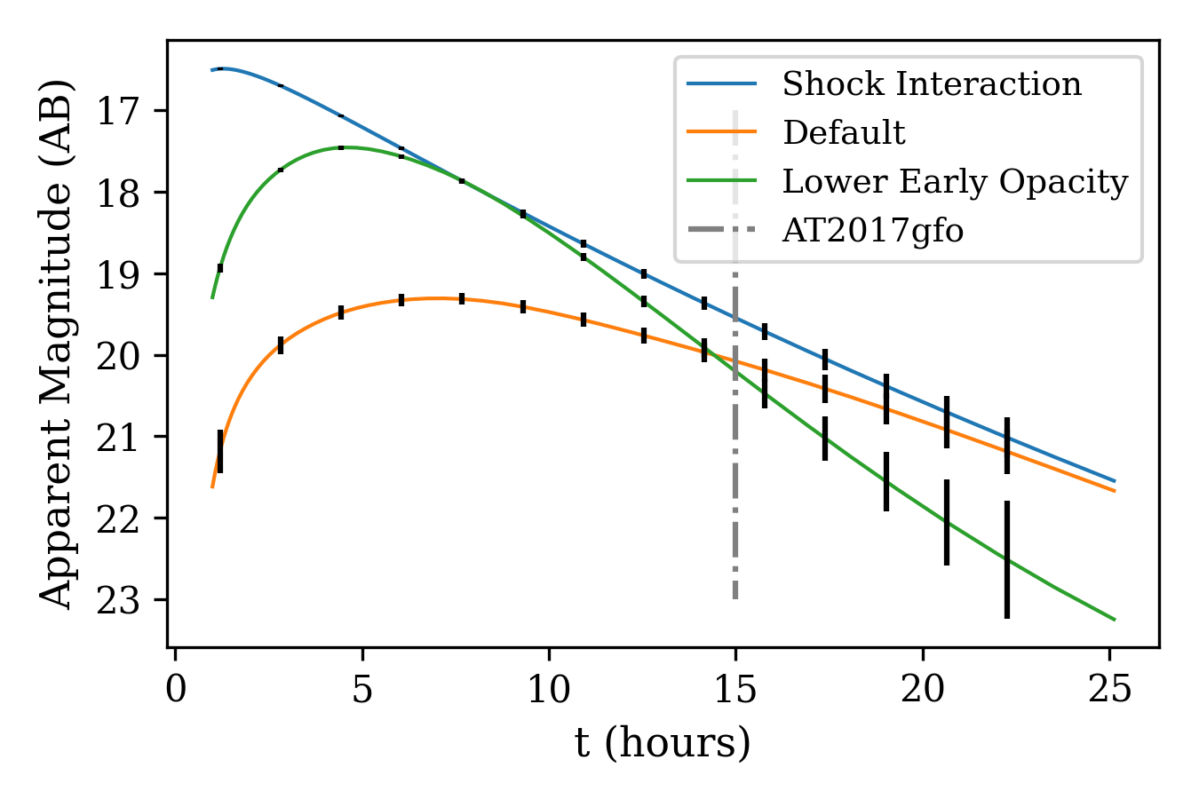
Figure 1: Comparison of AT2017gfo-like light curves in the Dorado UV band ($185215\text{\,}\mathrm{n}\mathrm{m}$) for kilonova models and shock interaction model at luminosity distance $d_{L}=$40\text{\,}\mathrm{M}\mathrm{p}\mathrm{c}$$. The data points correspond to 10 minute exposures that occur with a cadence of 97 minutes. There are fourteen data points in total for all light curves that are observed with identical timing. For reference, the dashdotted line indicates the timing of the first UV data recorded of AT2017gfo by Swift/UVOT at 15 hours (Evans et al., 2017).

The first fiducial light curve we call the ‘default’ light curve and is computed with the kilonova model using the same model parameters as Hotokezaka & Nakar (2020) to fit AT2017gfo. They found the resulting light curve to reasonably fit to the bolometric light curve and temperature data of AT2017gfo (taken from Arcavi, 2018; Waxman et al., 2018). The input parameters as well as prior distributions for the Bayesian analysis are given in Table 2.

Table 2: Input parameters to the kilonova and shock interaction models. On the left hand side, input parameter symbols are given along with units in parentheses. The prior density of the parameters are given in the third column, where the U(min, max) notation is used to indicate the minimum and maximum values of a uniform probability distribution. In the right hand column, the fiducial values for the fiducial light curves are given.

Parameter (Unit)	Description	Prior Density	Fiducial value
Default [Lower Early Opacity] Kilonova Model
$M_{\mathrm{ej}}$ (M⊙)	Ejecta mass	U(0.01, 0.1)	0.05
$v_{\mathrm{min}}$ (c)	Minimum ejecta velocity	U(0.05, 0.2)	0.1
$v_{\mathrm{max}}$ (c)	Maximum ejecta velocity	U(0.3, 0.8) [U(0.21, 0.8)]	0.4 [0.23]
$n_{\mathrm{ej}}$	Power law index of ejecta density distribution	U(3.5, 5)	4.5
$v_{\mathrm{transition}}$ (c)	Transition velocity between high and low $\kappa$	U($v_{\mathrm{min}}$, $v_{\mathrm{max}}$)	0.2 [0.2]
$\kappa_{\mathrm{high}}$ (cm2/g)	Effective grey opacity for $v\leq v_{\mathrm{\kappa}}$	U(1, 10)	3
$\kappa_{\mathrm{low}}$ (cm2/g)	Effective grey opacity for $v\geq v_{\mathrm{\kappa}}$	U(0.1, 1) [U(0.01, 0.1)]	0.5 [0.04]
Shock Interaction Powered Model
$M_{\mathrm{sh}}$ (M⊙)	Shocked ejecta mass	U(0.005, 0.05)	0.01
$v_{\mathrm{sh}}$[c]	Shocked ejecta minimum velocity	U(0.1, 0.3)	0.2
$R_{0}$ (1010 cm)	Initial shock radius	U(1, 10)	5
$\kappa_{\mathrm{sh}}$ (cm2/g)	Effective grey opacity of shocked ejecta	U(0.1, 1)	0.5

The second fiducial light curve is called the ‘lower early opacity’ light curve. Its inclusion here is motivated by recent work by Banerjee et al. (2020) who found light curves with early UV brightness that peak 1.5–2 magnitude brighter than the ‘default’ model. Rather than using a (multiple zone) gray opacity model, they performed a radiative transfer simulation using opacities calculated by taking into account atomic structures, including highly ionized light r-process elements ($Z=20-56$). The ‘lower early opacity’ light curve is a least squares fit with our kilonova model to both their simulated peak brightness and real Swift/UVOT data from AT2017gfo in AB magnitude. For this fit, we only allowed $v_{\rm transition}$, $v_{\rm max}$, $\kappa_{\rm low}$ to vary, which minimizes the change on the late time light curve while allowing for a good fit with the early UV light curve of Banerjee et al. (2020). The resulting $v_{\rm transition}$, $v_{\rm max}$, $\kappa_{\rm low}$ are shown in Table 2, but we find that $v_{\rm transition}$ remains the same. We also note that the AB magnitude of the ‘lower early opacity’ light curve at 0.1 day is brighter by $\sim$ 1 mag than the ‘light r-process+Sm+Nd+Eu’ model of Banerjee et al. (2022), where they perform a radiative transfer simulation accounting for the expansion opacities of highly ionized lanthanide elements. Thirdly and lastly, a fiducial light curve is produced by the shock interaction model. We use the fit to AT2017gfo provided by Piro & Kollmeier (2018) assuming $s=3$. These parameters too are given in Table 2.

3.3 Simulation of photometric data

Using all the fiducial light curves, we simulate photometric data as observed by Dorado in UV and by Las Cumbres Observatory (LCO) in the optical r-band. While more optical bands (such as u, g, and i) are available, we found that their inclusion minimally affected model selection and parameter estimation (compared to just the r-band) and omitted them in exchange for reduced computational time.

Dorado was a mission concept (Singer et al., 2021) consisting of a SmallSat (slightly larger than a 12U CubeSat) spacecraft equipped with a 13 cm refractive (7 element) telescope with a 50 deg² FoV. The instrument adopts a single (fixed) band-pass over the wavelength range from $185215\text{\,}\mathrm{n}\mathrm{m}$. The Dorado camera employs delta-doped charge coupled device (CCD) detectors to provide surface passivation and reflection-limited response over the UV bandpass (Nikzad et al., 2017). The spacecraft was designed to accommodate a wide range of low-Earth orbits and given ride-share availability we assume a noon-midnight sun synchronous (polar) orbit with a 600 km altitude for the simulations described here.

For the simulation of Dorado photometric data, representative observational cadences were derived using the dorado-scheduling software package. dorado-scheduling can generate realistic observational sequences for gravitational-wave localizations, including exclusion constraints (Sun, Moon, and Earth limb), as well as satellite down time for passages through the South Atlantic Anomaly. The software can define optimized observing strategies based on the GW localization region and distance, as well as a (position-dependent) exposure time calculator (see below). However, for these simulations we assumed the first data point is observed at $\Delta t=72$ min post merger (to allow for time to uplink to the spacecraft), and a fixed exposure time of 10 minutes every orbit (97 minute cadence) on a single pointing.

Signal-to-noise estimates were derived using the dorado-sensitivity, the exposure time calculator for the Dorado mission. dorado-sensitivity generates realistic foreground models for zodiacal light (based on spacecraft and target location), as well as airglow emission (based on location within the orbit). While the software is capable of incorporating Milky Way dust extinction, this is not included here. The fiducial light curve is folded through the Dorado effective area curve to generate the expected source counts, and then compared with the background (including both foreground and source shot noise). For reference, for a 10 minute exposure, Dorado’s 5$\sigma$ limiting magnitude for an isolated point source is typically $\sim$ 20.5 mag (AB).

For ground-based optical observations, we similarly use the same detection schedule for all simulated events but starting at 12 hours and with a 12 hour cadence up to 48 hours. To calculate this photometric data we use an exposure time calculator (ETC) constructed using data of LCO instruments. LCO is a network of 25 telescopes at seven sites around the world, sensitive in optical and NIR wavelengths. Being purpose-built to observe transient events, it robotically schedules observations and leverages its global network to observe around the clock and make rapid observations of targets of opportunity, evading potential local weather limitations (Brown et al., 2013).

4 Bayesian Analysis

This study employs Dynesty (Speagle, 2020) for Nested Sampling (Skilling, 2004, 2006). Nested Sampling is a method for simultaneously estimating posterior probability $P(\theta|D,M)$ (see Equation 6) and evidence $\mathcal{Z}$ (see Equation 7). The full pipeline for simulation of photometric data and subsequent Bayesian analysis is publicly available on Github. This section presents the results of the Bayesian analysis, and is structured as follows: Section 4.1 presents the results of model selection and parameter estimation via photometric data consisting of satellite-based UV, ground-based optical, and both. Section 4.2 considers satellite-based UV photometric data but analyzes the effect of delayed observation of the target.

4.1 Model Selection and Parameter Estimation for UV, Optical and Joint Data

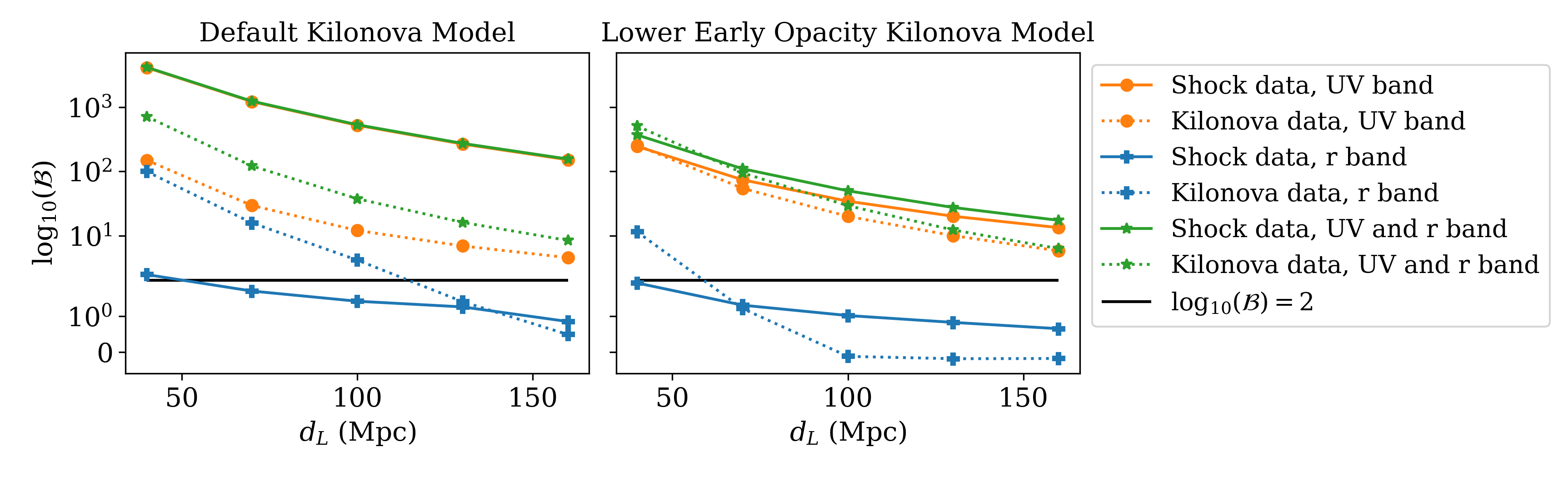
Figure 2: Bayes factors obtained from employing satellite-based UV, ground-based optical or joint UVO photometric data. Left: Resulting Bayes factors when attempting to distinguish the shock interaction model from ‘default’ kilonova model. Note here that the results obtained from shock data in UV+r bands overlap the results from the UV band. Right: Same, but now distinguishing the shock interaction model from the ‘lower early opacity’ kilonova model. The solid (dotted) lines correspond to Bayes factors resulting when using simulated data produced by the shock interaction model (kilonova model). The black horizontal line indicates the $\log_{10}(\mathcal{B})=2$ threshold for decisive evidence.

Figure 2 shows Bayes factors as a function of luminosity distance of the merger. In all cases up to $160\text{\,}\mathrm{M}\mathrm{p}\mathrm{c}$, the kilonova models can be confidently distinguished from the shock interaction model using only UV data. Conversely, the optical data is able to distinguish the models only up to $\sim$ 110 (60) $\mathrm{M}\mathrm{p}\mathrm{c}$ for the ‘default’ (‘lower early opacity’) light curves. Moreover, optical data produced by the shock interaction light curve presents edge cases at $40\text{\,}\mathrm{M}\mathrm{p}\mathrm{c}$ and beyond this distance the data is insufficient to distinguish the models. The combined UVO data set allows for (marginally) better distinguishability than the UV data.

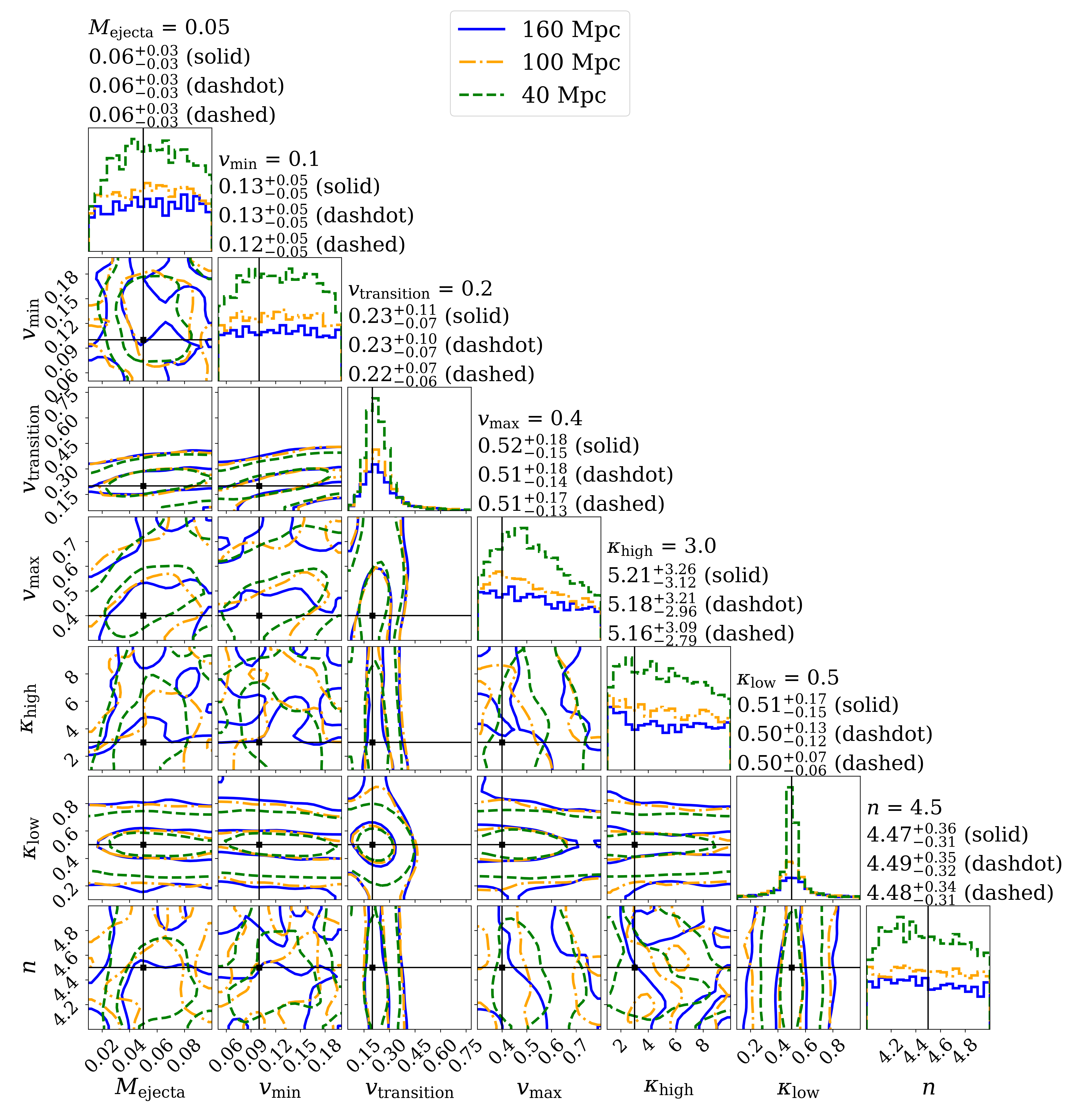
Figure 3: Posterior distributions of the parameters of the ‘default’ kilonova model, for an AT2017gfo-like event at $d_{L}$ = $40\text{\,}\mathrm{M}\mathrm{p}\mathrm{c}$, $100\text{\,}\mathrm{M}\mathrm{p}\mathrm{c}$ and $160\text{\,}\mathrm{M}\mathrm{p}\mathrm{c}$. The sub-figures on the diagonal of the corner plots display the PPD and the fiducial values for the model parameters (black lines). The sub-figure titles on the diagonal list the 0.16, 0.5, and 0.84 fractional quantiles. The contours in the 2D plots indicate the 2D 1$\sigma$ (39%) and 2$\sigma$ (86%) credible regions.

To get a handle on parameter estimation and its distance dependency, Figure 3 shows the posterior probability distributions (PPD) for the ‘default’ kilonova model at three selected luminosity distances: $d_{L}$ = $40\text{\,}\mathrm{M}\mathrm{p}\mathrm{c}$, $100\text{\,}\mathrm{M}\mathrm{p}\mathrm{c}$ and $160\text{\,}\mathrm{M}\mathrm{p}\mathrm{c}$. Two out of the seven model parameters: $v_{\mathrm{transition}}$ and $\kappa_{\mathrm{low}}$, are well constrained by the UV photometric data, but especially so at the most close-by distance at $40\text{\,}\mathrm{M}\mathrm{p}\mathrm{c}$. We note that these two parameters in part define the outer opacity zone of the ejecta outflow. Because the outer opacity zone is bright in UV (for these parameter values such that the light curves resemble AT2017gfo) we expect these parameters to be relatively well constrained by the UV photometric data. The remaining 5 parameters are not significantly constrained.

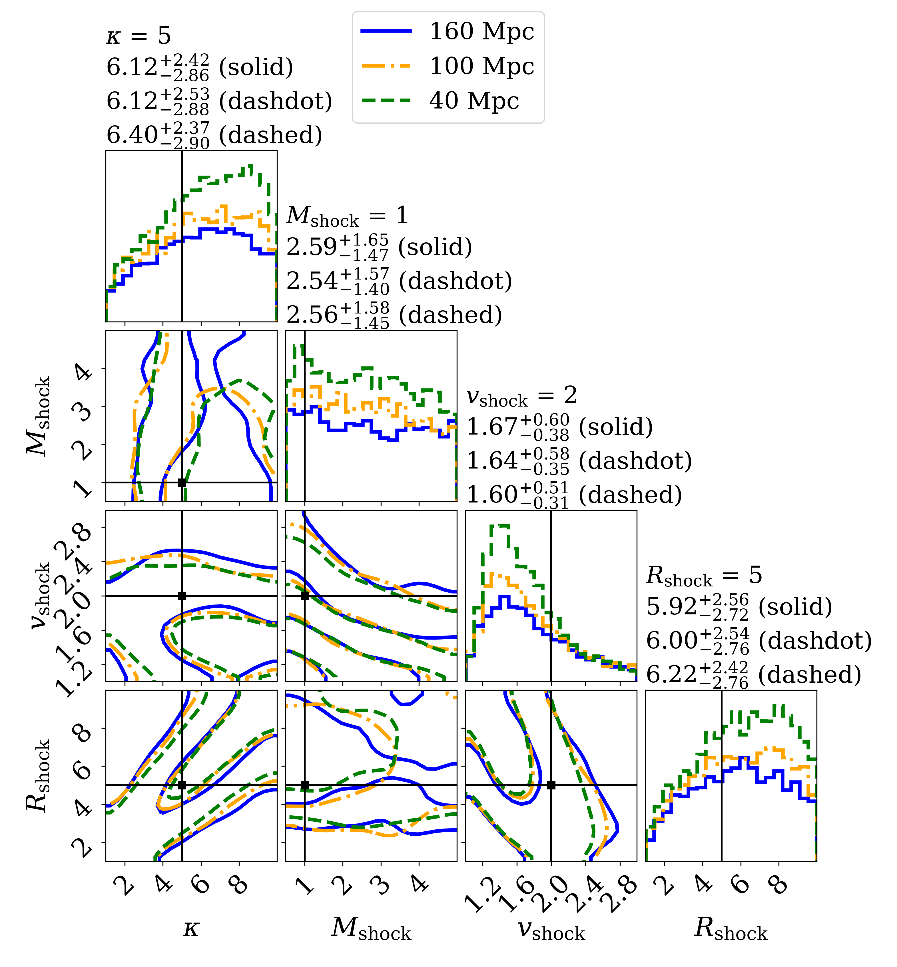
Figure 4: Same as Figure 3 but for the shock interaction model.

Figure 4 shows the PPD for the shock interaction model. Even for $40\text{\,}\mathrm{M}\mathrm{p}\mathrm{c}$ the parameters are constrained only slightly within prior ranges. As is evident from the figure, this lack in constraining of parameters is due to parameter degeneracy in this model. We find the following degeneracy in the model: consider a set of parameters $M_{1}$, $\kappa_{1}$ and $R_{1}$ that produce some $L_{1}$, $T_{\mathrm{eff},1}$ and $r_{\mathrm{ph},1}$. There exists another set of parameters, $M_{2}=\phi^{-1}M_{1}$, $\kappa_{2}=\phi\kappa_{1}$ and $R_{2}=\phi R_{1}$, where $\phi$ is some constant. Substituting these into Equations 3, 4 and 5, all factors $\phi$ cancel and we are left with $L_{1}=L_{2}$, $T_{\mathrm{eff},1}=T_{\mathrm{eff},2}$ and $r_{\mathrm{ph},1}=r_{\mathrm{ph},2}$. This means that the blackbody spectrum is identical for different parameters. Because of this degeneracy, parameters cannot be individually constrained even if observing in multiple bands. We note however, that in the case of AT2017gfo, the $R_{\mathrm{shock}}$ could be independently constrained from the time delay between GWs and GRB. In such a case $\kappa$ would become constrained, but a degeneracy remains between $M_{\rm shock}$ and $v_{\rm shock}$ ($M_{2}=\phi^{-4}M_{1}$ and $v_{2}=\phi v_{1}$).

Figure 5 shows the results for the ‘default’ kilonova model again (same as $40\text{\,}\mathrm{M}\mathrm{p}\mathrm{c}$ in Figure 3), but now also including a comparison with ground-based optical photometric data and with the combined data of both bands. In isolation ground-based optical observations constrain $M_{\mathrm{ejecta}}$ and $\kappa_{\mathrm{high}}$ more accurately and precisely than the UV. For $v_{\mathrm{min}},v_{\mathrm{transition}},v_{\mathrm{max}},\kappa_{\mathrm{high}}$ and $n$, performance of either single band is comparable, but constraints on $\kappa_{\mathrm{low}}$ are much worse for the optical than UV. However, in combination ground-based optical and UV are complementary to each other, providing significant improvement compared to using either band in isolation. In that case, all parameters except $n$ are well constrained.

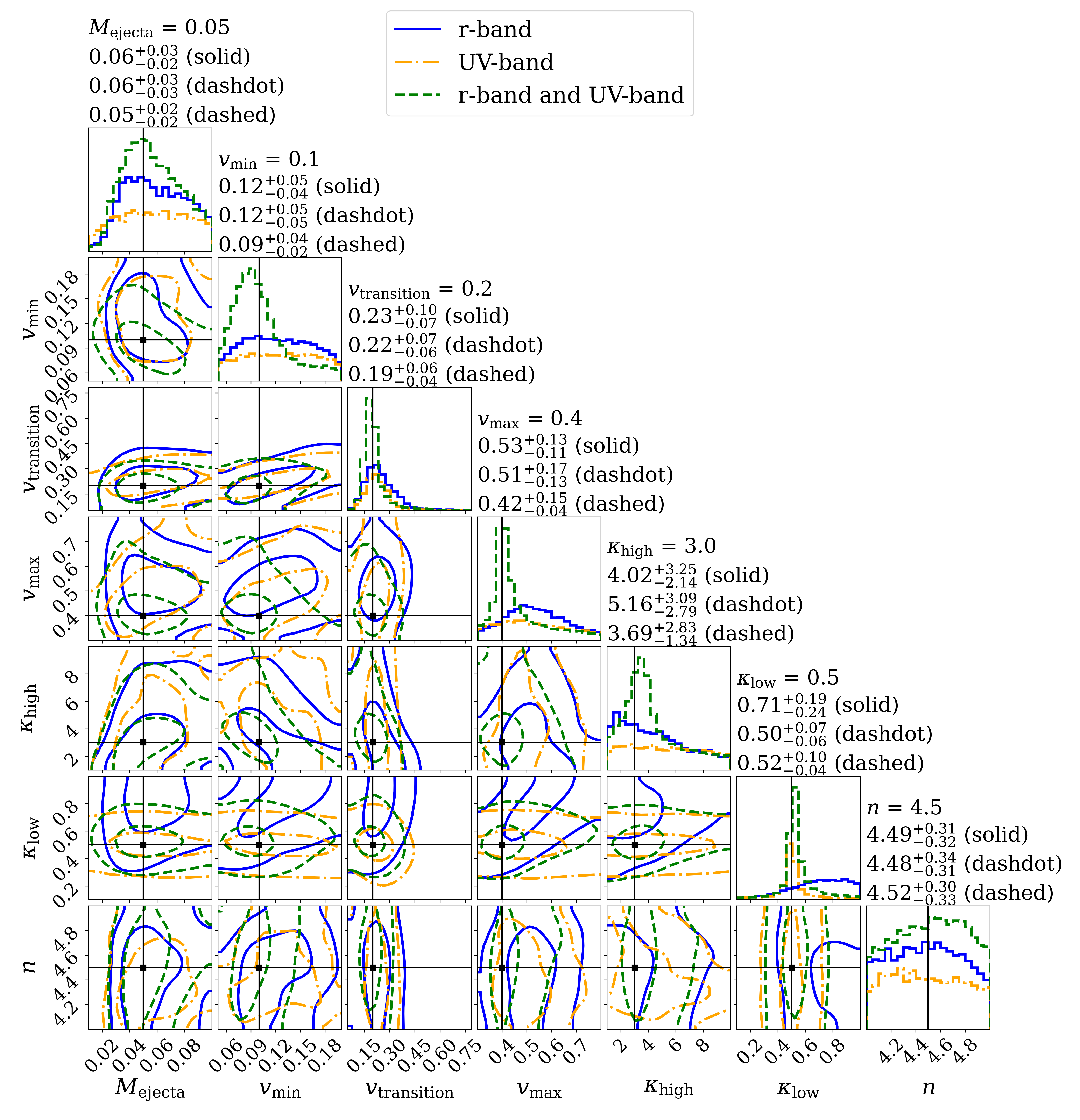
Figure 5: Similar to Figure 3, but now comparing results for parameter estimation using ground-based optical photometric data (solid), using satellite-based UV photometric data (dashdot) and both (dashed) for an event at $40\text{\,}\mathrm{M}\mathrm{p}\mathrm{c}$.

4.2 Delayed detection

The time it takes from GW trigger to first on-target exposure (effective response time) should be as short as possible to capture the physics that govern the early post-merger system. This is especially relevant for the UV compared to optical and IR because the emission rises and fades more rapidly ($\sim$ hours compared to $\sim$ days and $\sim\,$weeks respectively). Figure 6 shows the results for model selection using satellite-based UV photometric data, where the data set as a whole was shifted forwards in time with various delays as indicated in the figure. Note that the cases for data at $1.2\text{\,}\mathrm{h}$ are identical to the UV data in Figure 2. For distances up to $160\text{\,}\mathrm{M}\mathrm{p}\mathrm{c}$, it is possible to distinguish the models if the first data is collected up to 5.2 (3.2) hours after GW trigger for the ‘default’ (‘lower early opacity’) light curves. For $40\text{\,}\mathrm{M}\mathrm{p}\mathrm{c}$ and beyond, the models cannot be distinguished if the first data is collected after 13.2 hours.

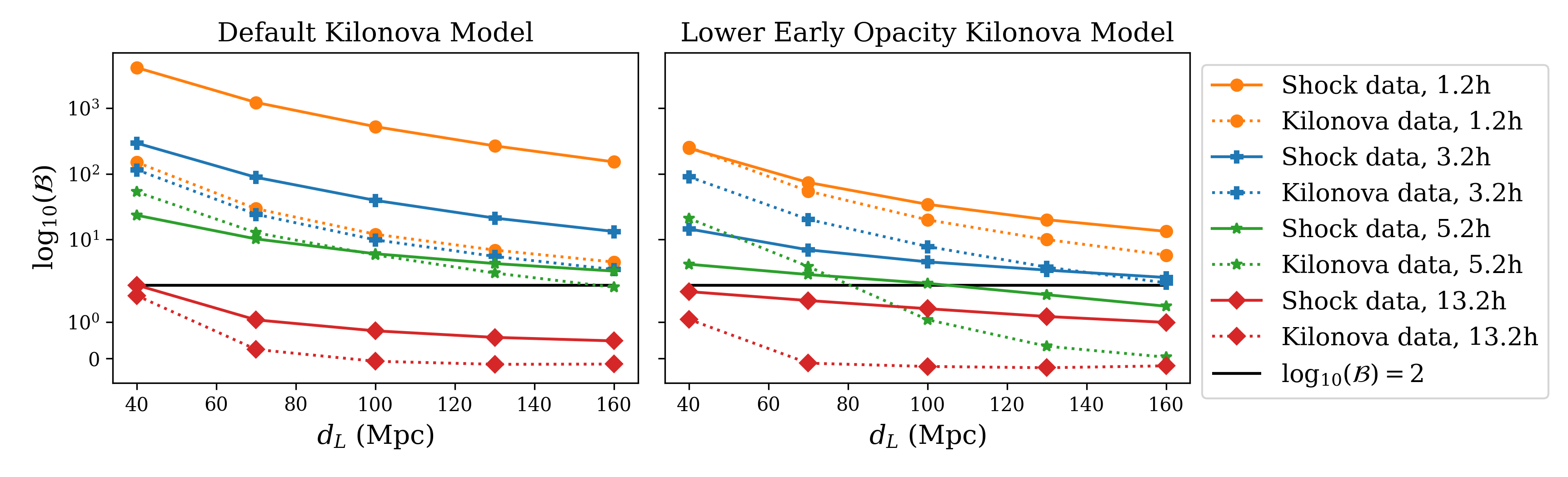
Figure 6: Bayes factors obtained from model selection using satellite-based UV photometric data. The data is shifted in time such that the first data point is obtained at $1.2$, $3.2$, $5.2$ and $13.2$ hours after GW trigger. The distinction between left and right, dotted and solid lines as well as the black horizontal line are explained in the caption of Figure 2.

Figure 7 shows the results for parameter estimation for increasingly delayed photometric data. Note that the results for $1.2\text{\,}\mathrm{h}$ are identical to $40\text{\,}\mathrm{M}\mathrm{p}\mathrm{c}$ in Figure 3. All parameters experience worsening constraints for increasing response time. Of the two parameters that were previously well constrained for satellite-based UV photometric data, $v_{\mathrm{transition}}$ is still well constrained even for data starting at $25.2\text{\,}\mathrm{h}$ while $\kappa_{\mathrm{low}}$ is not well constrained beyond $13.2\text{\,}\mathrm{h}$. We posit that $v_{\mathrm{transition}}$ may be well constrained even with such delayed data because it affects both opacity zones, while $\kappa_{\mathrm{low}}$ only plays a role in defining the quicker fading outer opacity zone.

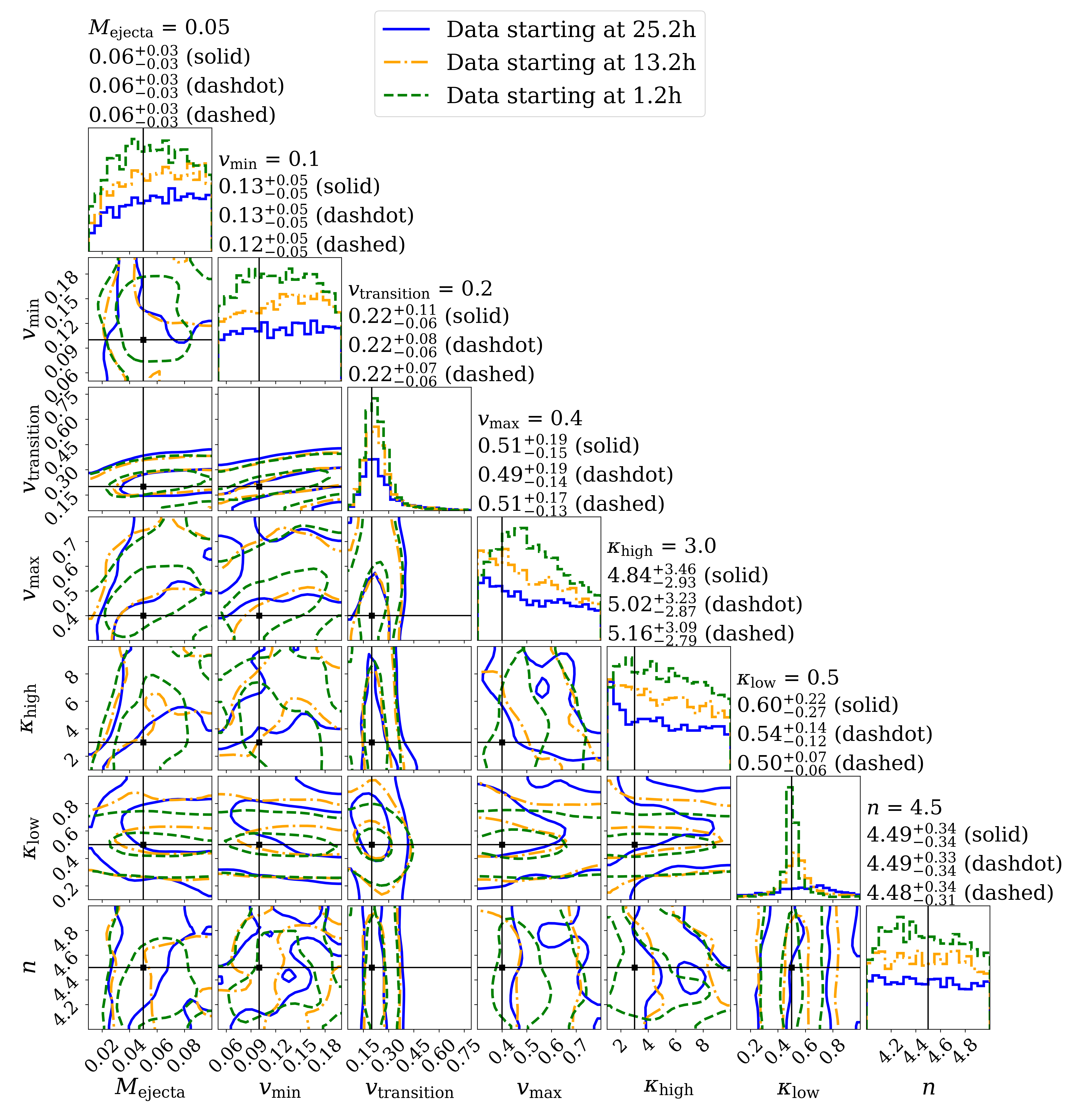
Figure 7: Similar to Figure 3, but now with the satellite-based UV photometric data at $40\text{\,}\mathrm{M}\mathrm{p}\mathrm{c}$ shifted in time such that the first data point is obtained at $1.2$, $13.2$ and $25.2$ hours.

5 Discussion and Conclusion

We have performed model selection and parameter estimation, assuming AT2017gfo-like ‘blue’ emission produced by either kilonova or shock interaction radiation and assuming observational capabilities of a UV satellite (Dorado) and a ground-based observation network (LCO). Our main findings are threefold:

Firstly, our results suggest that satellite-based UV photometric data, unaided by ground-based optical follow-up would be sufficient to distinguish these models for an event up to at least $160\text{\,}\mathrm{M}\mathrm{p}\mathrm{c}$ for all considered scenarios. Conversely, ground-based optical photometric data only selects models up to $\sim$ $110\text{\,}\mathrm{M}\mathrm{p}\mathrm{c}$ in the most optimistic scenario and has considerably worse performance ($\sim$ $40\text{\,}\mathrm{M}\mathrm{p}\mathrm{c}$) in other scenarios. Combined UVO photometric data only marginally improves model selection beyond what is possible with only UV data.

Secondly, we find that combined UVO photometric data allows the full set of parameters (save $n$, which defines steepness of the ejecta velocity profile) of our kilonova model to be well constrained. In comparison, photometric data from either UV or optical alone constrains smaller subsets of the parameters and with reduced accuracy and precision. This result suggests that multiple-wavelength detections are essential for constraining early ejecta geometry and opacity.

Thirdly, we find that the data allows to discern between the models if first data is observed no later than 3.2 (5.2) hours after GW trigger for the ‘default’ (‘lower early opacity’) light curves up to $160\text{\,}\mathrm{M}\mathrm{p}\mathrm{c}$. Moreover, after $13.2\text{\,}\mathrm{h}$ the models can no longer be discerned beyond $40\text{\,}\mathrm{M}\mathrm{p}\mathrm{c}$. These results indicate that rapid on-target observations on the order of a few hours is necessary for distinguishing the kilonova from shock interaction models through UV photometric data.

To place these results in broader context, we comment on prospects for planned wide-field UV instruments to detect and characterize EM counterparts during the O5 observation run of GW observatories Advanced LIGO, Virgo and KAGRA (HLVK) in 2024 and beyond. We focus here on O5, because the launch dates of ULTRASAT (2025) and UVEX ($\sim$ 2028) are in part overlapping with O5.

Simulations of GW detections in O5 were done by Petrov et al. (2022). From their simulated data set (Singer, 2021) we compute that of BNS events within 160 Mpc, 69% are localized within 100 deg², which would be easily followed up by Dorado within a single orbit. The fraction of events that meet both distance and localization criteria, multiplied by the annual detection rate (190, from Petrov et al. (2022)) gives an annual detection rate of $\sim$ 3.2. If we include events up to 400 Mpc, we find that still 46% of events are localized within 100 deg², corresponding to an annual rate of $\sim$ 20 events. Thus, for BNS mergers, if we assume similar brightness to AT2017gfo (see below), we expect an annual detection rate of $\sim$ $3.2$ of which shock interaction and kilonova radiation could be distinguished and kilonova ejecta parameters constrained with a Dorado-like satellite. For BHNS mergers, which have not been simulated here, the expected number of detected EM counterparts should be much lower, as only a small region of BHNS parameter space will lead to disruption of the NS (Foucart, 2020). While the simulations performed here are specific to Dorado, some of the findings also are relevant to currently planned wide-field UV missions. To start with, the wide-field UV mission ULTRASAT is more sensitive than Dorado with a limiting magnitude of $\sim$ 22.3 (5$\sigma$, AB, 3$\times$$300\text{\,}\mathrm{s}$ exposure) and has a larger FoV at 200 deg² (Asif et al., 2021). Because of this, and ULTRASATs ability to point to a given ToO within 30 minutes (Sagiv et al., 2014), it is both sensitive and quick enough to provide the UV data for model selection and constraints as suggested by simulations here. Secondly, UVEX is even more sensitive with a limiting magnitude of 25 (AB, 5$\sigma$) but has a smaller FoV of 12 deg². In addition, UVEX will provide additional detail in the light curves and spectra through its two (far and near UV) sensors and on-board spectroscope (Kulkarni et al., 2021). Because this mission has additional capabilities, applicability of these results to this mission is not straightforward. For both we recommend separate simulations that accurately represent their mission parameters to assess capability for model distinction and parameter estimation.

Finally, we remark on the various simplifying assumptions made in this study that may affect the robustness of above findings. To start with, throughout this work we have made the assumption that the EM counterparts of BNS mergers all are similar to that of AT2017gfo. This introduces a ‘AT2017gfo-bias’ in our predictions for the ability of a future UV satellite to achieve science goals. It is as of yet uncertain how representative AT2017gfo is for the actual kilonova population and O4 and O5 are expected to shed light on this. This population is expected to be diverse, for example due to binary properties such as mass ratio and spins, but also post-merger properties such as remnant outcome (e.g. Kawaguchi et al., 2020) and jet-ejecta interaction (e.g. Klion et al., 2021). These are expected to have an effect on ejecta geometry and composition which in turn affects brightness and color of light curves.

Another assumption underlying this study is that both models assume isotropic ejecta. However, the photon emission as well as composition and geometry of the ejecta are not expected to be spherically symmetric (e.g. Metzger, 2017; Heinzel et al., 2021). Other models that include the inclination angle, such as the grid of 2D simulations presented by Wollaeger et al. (2021), would allow for a more representative study covering the angular dependence of UV light curves. Still, Heinzel et al. (2021) recommend the inclusion of $\sim$ 1 mag uncertainties for kilonova models used in Bayesian studies relating to inclination angle to capture yet unknown systematic model uncertainties.

We also note that a significant source of uncertainty remains in the nuclear physics taking place in these high energy events. For example, Zhu et al. (2022) find that uncertainties in nuclear inputs lead to typically one order of magnitude variation in inferred nuclear heating, bolometric luminosity and ejecta mass.

Lastly, although the scope of this study was limited to shock interaction and kilonova radiation, we note that a more comprehensive study may include additional radiation scenarios, such as a neutron precursor or winds driven by a long-lived remnant, and also a combination of emission channels.

In conclusion, these results show that UV data offers a unique window to distinguish the processes governing the early post-merger system. For Dorado, rapid follow-up as well as the ability to quickly localize the target within a few hours catches the quickly fading UV emission, allowing to distinguish models. We also find that through multi-wavelength observations the kilonova emission can be constrained up to at least $160\text{\,}\mathrm{M}\mathrm{p}\mathrm{c}$, unlocking a fuller understanding of the geometry and opacity of the ejecta outflow.

BD is grateful to the whole Dorado team for their development of the mission concept, which enabled this detailed case study. BD acknowledges support from ERC Consolidator grant No. 865768 AEONS (PI: Anna Watts).

References

- Abbott et al. (2017a) Abbott, B. P., Abbott, R., Abbott, T. D., et al. 2017a, Phys. Rev. Lett., 119, 161101, doi: 10.1103/PhysRevLett.119.161101
- Abbott et al. (2017b) —. 2017b, ApJ, 848, L12, doi: 10.3847/2041-8213/aa91c9
- Abbott et al. (2017c) —. 2017c, ApJ, 848, L13, doi: 10.3847/2041-8213/aa920c
- Abbott et al. (2020) —. 2020, Living Reviews in Relativity, 23, 3, doi: 10.1007/s41114-020-00026-9
- Arcavi (2018) Arcavi, I. 2018, ApJ, 855, L23, doi: 10.3847/2041-8213/aab267
- Arcavi et al. (2017) Arcavi, I., McCully, C., Hosseinzadeh, G., et al. 2017, ApJ, 848, L33, doi: 10.3847/2041-8213/aa910f
- Arnett (1982) Arnett, W. D. 1982, ApJ, 253, 785, doi: 10.1086/159681
- Asif et al. (2021) Asif, A., Barschke, M., Bastian-Querner, B., et al. 2021, in Society of Photo-Optical Instrumentation Engineers (SPIE) Conference Series, Vol. 11821, Society of Photo-Optical Instrumentation Engineers (SPIE) Conference Series, 118210U, doi: 10.1117/12.2594253
- Banerjee et al. (2022) Banerjee, S., Tanaka, M., Kato, D., et al. 2022, Opacity of the highly ionized lanthanides and the effect on the early kilonova, arXiv, doi: 10.48550/ARXIV.2204.06861
- Banerjee et al. (2020) Banerjee, S., Tanaka, M., Kawaguchi, K., Kato, D., & Gaigalas, G. 2020, ApJ, 901, 29, doi: 10.3847/1538-4357/abae61
- Brown et al. (2013) Brown, T. M., Baliber, N., Bianco, F. B., et al. 2013, PASP, 125, 1031, doi: 10.1086/673168
- Chase et al. (2022) Chase, E. A., O’Connor, B., Fryer, C. L., et al. 2022, ApJ, 927, 163, doi: 10.3847/1538-4357/ac3d25
- Chornock et al. (2017) Chornock, R., Berger, E., Kasen, D., et al. 2017, ApJ, 848, L19, doi: 10.3847/2041-8213/aa905c
- Coulter et al. (2017) Coulter, D. A., Foley, R. J., Kilpatrick, C. D., et al. 2017, Science, 358, 1556, doi: 10.1126/science.aap9811
- Cowperthwaite et al. (2017) Cowperthwaite, P. S., Berger, E., Villar, V. A., et al. 2017, ApJ, 848, L17, doi: 10.3847/2041-8213/aa8fc7
- Droettboom et al. (2018) Droettboom, M., Caswell, T. A., Hunter, J., et al. 2018, Matplotlib/Matplotlib V2.2.2, v2.2.2, Zenodo, Zenodo, doi: 10.5281/zenodo.1202077
- Drout et al. (2017) Drout, M. R., Piro, A. L., Shappee, B. J., et al. 2017, Science, 358, 1570, doi: 10.1126/science.aaq0049
- Evans et al. (2017) Evans, P. A., Cenko, S. B., Kennea, J. A., et al. 2017, Science, 358, 1565, doi: 10.1126/science.aap9580
- Foreman-Mackey (2016) Foreman-Mackey, D. 2016, The Journal of Open Source Software, 1, 24, doi: 10.21105/joss.00024
- Foucart (2020) Foucart, F. 2020, Frontiers in Astronomy and Space Sciences, 7, 46, doi: 10.3389/fspas.2020.00046
- Goldstein et al. (2017) Goldstein, A., Veres, P., Burns, E., et al. 2017, ApJ, 848, L14, doi: 10.3847/2041-8213/aa8f41
- Gottlieb & Loeb (2020) Gottlieb, O., & Loeb, A. 2020, MNRAS, 493, 1753, doi: 10.1093/mnras/staa363
- Heinzel et al. (2021) Heinzel, J., Coughlin, M. W., Dietrich, T., et al. 2021, MNRAS, 502, 3057, doi: 10.1093/mnras/stab221
- Hotokezaka & Nakar (2020) Hotokezaka, K., & Nakar, E. 2020, ApJ, 891, 152, doi: 10.3847/1538-4357/ab6a98
- Hunter (2007) Hunter, J. D. 2007, Computing in Science and Engineering, 9, 90, doi: 10.1109/MCSE.2007.55
- Jones et al. (2001–) Jones, E., Oliphant, T., Peterson, P., et al. 2001–, SciPy: Open source scientific tools for Python. http://www.scipy.org/
- Kasen et al. (2013) Kasen, D., Badnell, N. R., & Barnes, J. 2013, ApJ, 774, 25, doi: 10.1088/0004-637X/774/1/25
- Kasen & Barnes (2019) Kasen, D., & Barnes, J. 2019, ApJ, 876, 128, doi: 10.3847/1538-4357/ab06c2
- Kasen et al. (2017) Kasen, D., Metzger, B., Barnes, J., Quataert, E., & Ramirez-Ruiz, E. 2017, Nature, 551, 80, doi: 10.1038/nature24453
- Kasliwal et al. (2017) Kasliwal, M. M., Nakar, E., Singer, L. P., et al. 2017, Science, 358, 1559, doi: 10.1126/science.aap9455
- Kass & Raftery (1995) Kass, R. E., & Raftery, A. E. 1995, Journal of the American Statistical Association, 90, 773, doi: 10.1080/01621459.1995.10476572
- Kawaguchi et al. (2020) Kawaguchi, K., Shibata, M., & Tanaka, M. 2020, ApJ, 893, 153, doi: 10.3847/1538-4357/ab8309
- Klion et al. (2021) Klion, H., Duffell, P. C., Kasen, D., & Quataert, E. 2021, MNRAS, 502, 865, doi: 10.1093/mnras/stab042
- Kluyver et al. (2016) Kluyver, T., Ragan-Kelley, B., Pérez, F., et al. 2016, in Positioning and Power in Academic Publishing: Players, Agents and Agendas, ed. F. Loizides & B. Schmidt, IOS Press, 87 – 90
- Kulkarni (2005) Kulkarni, S. R. 2005, arXiv e-prints, astro. https://arxiv.org/abs/astro-ph/0510256
- Kulkarni et al. (2021) Kulkarni, S. R., Harrison, F. A., Grefenstette, B. W., et al. 2021, arXiv e-prints, arXiv:2111.15608. https://arxiv.org/abs/2111.15608
- Lattimer & Schramm (1974) Lattimer, J. M., & Schramm, D. N. 1974, ApJ, 192, L145, doi: 10.1086/181612
- Li & Paczyński (1998) Li, L.-X., & Paczyński, B. 1998, ApJ, 507, L59, doi: 10.1086/311680
- Lipunov et al. (2017) Lipunov, V. M., Gorbovskoy, E., Kornilov, V. G., et al. 2017, ApJ, 850, L1, doi: 10.3847/2041-8213/aa92c0
- McCully et al. (2017) McCully, C., Hiramatsu, D., Howell, D. A., et al. 2017, ApJ, 848, L32, doi: 10.3847/2041-8213/aa9111
- Metzger (2017) Metzger, B. D. 2017, Living Reviews in Relativity, 20, 3, doi: 10.1007/s41114-017-0006-z
- Metzger et al. (2015) Metzger, B. D., Bauswein, A., Goriely, S., & Kasen, D. 2015, MNRAS, 446, 1115, doi: 10.1093/mnras/stu2225
- Metzger et al. (2018) Metzger, B. D., Thompson, T. A., & Quataert, E. 2018, ApJ, 856, 101, doi: 10.3847/1538-4357/aab095
- Metzger et al. (2010) Metzger, B. D., Martínez-Pinedo, G., Darbha, S., et al. 2010, MNRAS, 406, 2650, doi: 10.1111/j.1365-2966.2010.16864.x
- Nakar (2020) Nakar, E. 2020, Phys. Rep., 886, 1, doi: 10.1016/j.physrep.2020.08.008
- Nakar & Piran (2017) Nakar, E., & Piran, T. 2017, ApJ, 834, 28, doi: 10.3847/1538-4357/834/1/28
- Nedora et al. (2021) Nedora, V., Bernuzzi, S., Radice, D., et al. 2021, ApJ, 906, 98, doi: 10.3847/1538-4357/abc9be
- Nicholl et al. (2017) Nicholl, M., Berger, E., Kasen, D., et al. 2017, ApJ, 848, L18, doi: 10.3847/2041-8213/aa9029
- Nikzad et al. (2017) Nikzad, S., Jewell, A. D., Hoenk, M. E., et al. 2017, Journal of Astronomical Telescopes, Instruments, and Systems, 3, 036002, doi: 10.1117/1.JATIS.3.3.036002
- Oliphant (2007) Oliphant, T. E. 2007, Computing in Science and Engineering, 9, 10, doi: 10.1109/MCSE.2007.58
- Perez & Granger (2007) Perez, F., & Granger, B. E. 2007, Computing in Science and Engineering, 9, 21, doi: 10.1109/MCSE.2007.53
- Petrov et al. (2022) Petrov, P., Singer, L. P., Coughlin, M. W., et al. 2022, ApJ, 924, 54, doi: 10.3847/1538-4357/ac366d
- Piro & Kollmeier (2018) Piro, A. L., & Kollmeier, J. A. 2018, ApJ, 855, 103, doi: 10.3847/1538-4357/aaaab3
- Rosswog et al. (2017) Rosswog, S., Feindt, U., Korobkin, O., et al. 2017, Classical and Quantum Gravity, 34, 104001, doi: 10.1088/1361-6382/aa68a9
- Sagiv et al. (2014) Sagiv, I., Gal-Yam, A., Ofek, E. O., et al. 2014, AJ, 147, 79, doi: 10.1088/0004-6256/147/4/79
- Savchenko et al. (2017) Savchenko, V., Ferrigno, C., Kuulkers, E., et al. 2017, ApJ, 848, L15, doi: 10.3847/2041-8213/aa8f94
- Shappee et al. (2017) Shappee, B. J., Simon, J. D., Drout, M. R., et al. 2017, Science, 358, 1574, doi: 10.1126/science.aaq0186
- Shibata et al. (2017) Shibata, M., Fujibayashi, S., Hotokezaka, K., et al. 2017, Phys. Rev. D, 96, 123012, doi: 10.1103/PhysRevD.96.123012
- Singer (2021) Singer, L. 2021, Data-driven expectations for electromagnetic counterpart searches based on LIGO/Virgo public alerts: O5 simulations, Zenodo, doi: 10.5281/zenodo.4765752
- Singer et al. (2021) Singer, L. P., Cenko, S., & Dorado Science Team. 2021, in American Astronomical Society Meeting Abstracts, Vol. 53, American Astronomical Society Meeting Abstracts, 309.05
- Sivia & Skilling (2006) Sivia, D., & Skilling, J. 2006, Data analysis: a Bayesian tutorial (OUP Oxford)
- Skilling (2004) Skilling, J. 2004, in American Institute of Physics Conference Series, Vol. 735, Bayesian Inference and Maximum Entropy Methods in Science and Engineering: 24th International Workshop on Bayesian Inference and Maximum Entropy Methods in Science and Engineering, ed. R. Fischer, R. Preuss, & U. V. Toussaint, 395–405, doi: 10.1063/1.1835238
- Skilling (2006) Skilling, J. 2006, Bayesian Analysis, 1, 833 , doi: 10.1214/06-BA127
- Soares-Santos et al. (2017) Soares-Santos, M., Holz, D. E., Annis, J., et al. 2017, ApJ, 848, L16, doi: 10.3847/2041-8213/aa9059
- Speagle (2020) Speagle, J. S. 2020, MNRAS, 493, 3132, doi: 10.1093/mnras/staa278
- Tanaka & Hotokezaka (2013) Tanaka, M., & Hotokezaka, K. 2013, ApJ, 775, 113, doi: 10.1088/0004-637X/775/2/113
- Tanaka et al. (2020) Tanaka, M., Kato, D., Gaigalas, G., & Kawaguchi, K. 2020, MNRAS, 496, 1369, doi: 10.1093/mnras/staa1576
- Tanaka et al. (2017) Tanaka, M., Utsumi, Y., Mazzali, P. A., et al. 2017, PASJ, 69, 102, doi: 10.1093/pasj/psx121
- Tange (2021) Tange, O. 2021, GNU Parallel 20211222 (’Støjberg’), Zenodo, doi: 10.5281/zenodo.5797028
- Valenti et al. (2017) Valenti, S., Sand, D. J., Yang, S., et al. 2017, ApJ, 848, L24, doi: 10.3847/2041-8213/aa8edf
- van der Walt et al. (2011) van der Walt, S., Colbert, S. C., & Varoquaux, G. 2011, Computing in Science and Engineering, 13, 22, doi: 10.1109/MCSE.2011.37
- Villar et al. (2017) Villar, V. A., Guillochon, J., Berger, E., et al. 2017, ApJ, 851, L21, doi: 10.3847/2041-8213/aa9c84
- Waxman et al. (2019) Waxman, E., Ofek, E. O., & Kushnir, D. 2019, ApJ, 878, 93, doi: 10.3847/1538-4357/ab1f71
- Waxman et al. (2018) Waxman, E., Ofek, E. O., Kushnir, D., & Gal-Yam, A. 2018, MNRAS, 481, 3423, doi: 10.1093/mnras/sty2441
- Wollaeger et al. (2018) Wollaeger, R. T., Korobkin, O., Fontes, C. J., et al. 2018, MNRAS, 478, 3298, doi: 10.1093/mnras/sty1018
- Wollaeger et al. (2021) Wollaeger, R. T., Fryer, C. L., Chase, E. A., et al. 2021, ApJ, 918, 10, doi: 10.3847/1538-4357/ac0d03
- Zhu et al. (2022) Zhu, Y., Barnes, J., Lund, K. A., et al. 2022, in European Physical Journal Web of Conferences, Vol. 260, European Physical Journal Web of Conferences, 03004, doi: 10.1051/epjconf/202226003004