Threshold transient growth as a criterion for turbulent mean profiles

Abstract

Lozano-Duran et al (J. Fluid Mech., 914, A8, 2021) have recently identified the ability of streamwise-averaged turbulent streak fields ${\cal U}(y,z,t)\hat{\mbox{\boldmath$x$}}$ in minimal channels to produce short-term transient growth as the key linear mechanism needed to sustain turbulence at $Re_{\tau}=180$. Here, we model this streak transient growth as a two-stage linear process by first selecting the dominant streak structure expected to emerge over the eddy turnover time on the turbulent mean profile $U(y)\hat{\mbox{\boldmath$x$}}$, and then examining the secondary growth on this (frozen) streak field ${\cal U}(y,z)\hat{\mbox{\boldmath$x$}}$. Choosing the mean streak amplitude and eddy turnover time consistent with simulations recovers the growth thresholds found by Lozano-Duran et al. (2021) for sustained turbulence. Interestingly, even more growth is possible for less-optimal streaks of approximately double the spanwise wavelength at the larger amplitudes found in simulations. This most energetic streak spacing, however, starts to approach the optimal streak in a larger geometry at higher $Re_{\tau}$ where the growth possible on each also comes together. Our results feed into the idea that the short-term perturbation growth properties of the turbulent mean profile is a much more plausible criterion of turbulence existence than the asymptotic (linear) stability as originally suggested by Malkus (J. Fluid Mech., 521, 1, 1956).

1 Introduction

In turbulent wall-bounded shear flows, only the mean flow is energised by external driving effects and so it has to pass on some of its energy to the fluctuation field. Linearising the Navier-Stokes equations around the mean velocity profile is sufficient to capture all the possible energy transfer processes. Hence, linear models based on modal stability analysis or transient growth are popular tools used in flow control (Kim & Bewley, 2007; Rowley & Dawson, 2017). Recently, in a comprehensive cause-and-effect study, Lozano-Duran et al. (2021) (hereafter LD21) identified that transient growth around the streamwise-averaged velocity profile is the essential linear mechanism needed to sustain turbulence in plane channel flow with a particular threshold of the growth needed to sustain the turbulence at $Re_{\tau}=180$ in a minimal flow unit. This result hints at a possible and interesting update on Malkus’s (1956) well-known but defunct hypothesis that the turbulent mean profile $U(y)\hat{\mbox{\boldmath$x$}}$ (where $x$ is the streamwise and $y$ the cross-shear directions) is marginally (linearly) stable. Instead, the result of LD21 suggests that there may be some sort of statistical (linear) transient growth threshold on the extended mean profiles ${\cal U}(y,z,t)\hat{\mbox{\boldmath$x$}}$ (where $z$ is the spanwise direction) realised in the flow (‘statistical’ here means in some averaged sense over the family of realised profiles ${\cal U}(y,z,t)$ parametrised by time $t$ rather than ‘statistical stability’ ideas considered in Markeviciute & Kerswell (2023)). An alternative perspective is that the mean $U(y)\hat{\mbox{\boldmath$x$}}$ has a threshold for nonlinear transient growth where the growth possible for perturbations of a finite amplitude ( the amplitude of the observed streak field ${\cal U}(y,z,t)-U(y)$ ) have to be considered.

The work of LD21 needs extending, however, to larger flow domains to test robustness and higher $Re_{\tau}$ to reveal how the threshold growth possibly scales. Unfortunately, the amount of computation involved is forbidding which suggests trying to identify and study a theoretical proxy. So motivated, we build a simple two-stage model of primary and secondary linear transient growth here and use this to suggest how LD21’s results would generalise. The primary linear process is the energy transfer from the streamwise- and spanwise-averaged velocity profile $U(y)\hat{\mbox{\boldmath$x$}}$ via streamwise rolls to spanwise-dependent but streamwise-independent streaks ${\bf\cal U}(y,z,t)\hat{\mbox{\boldmath$x$}}$ due to the non-normality of the linear operator. This transient growth process is now well understood (e.g. Orr (1907); Farrell (1988) for laminar flows and Kim & Lim (2000); del Alamo & Jimenez (2006); Cossu et al. (2009) in turbulent settings). The streak formation can also be explained through a stable mode in statistically forced turbulence modelled with Statistical State Dynamics (SSD) (Farrell et al., 2017), or by the pattern forming properties of the lift-up, shear and diffusion of the mean profile (Chernyshenko & Baig, 2005). Most notably, Butler & Farrell (1993) were able to show that the observed spanwise streak spacing was consistent with optimal disturbances constrained to grow maximally over an eddy turnover time.

Taking the new base flow as the final primary streak structure added to the mean velocity profile, the secondary linear process can be considered to model the subsequent streak breakdown. The exact linear mechanism driving the breakdown has been widely discussed. While some studies emphasised the importance of the modal instability of the streaks (Hamilton et al., 1995; Andersson et al., 2001), Schoppa & Hussain (2002) showed that most of the streaks observed in simulations are in fact exponentially stable and suggested transient growth as the driving mechanism of streak breakdown. The feasibility of this conclusion was debated (Jiménez, 2018) and alternative explanations such as parametric streak instability considered (Farrell & Ioannou, 1999; Farrell et al., 2016). Recently, in their exhaustive cause-and-effect study of possible secondary linear mechanisms, LD21 showed that transient growth fuelled by ‘push-over’ and Orr mechanisms (Orr, 1907) is the necessary ingredient in sustaining turbulence in minimal channels at least at $Re_{\tau}=180$. However, it remains unknown what perturbations and primary streak amplitudes lead to transient growth levels sufficient to sustain turbulence, the understanding of which could enhance flow control strategies. Previous work in this direction is mainly DNS-based including the direct-adjoint looping optimisation of the non-linear Navier-Stokes equations around a laminar Poiseuille profile with varying amplitude streak (Cossu et al., 2007).

In this paper we design a two-stage transient growth process to study the optimal perturbation energy gain starting from a $U(y)\hat{\mbox{\boldmath$x$}}$ mean flow generated by DNS in a minimal channel. A (primary) transient growth calculation is then performed in the same spirit as Butler & Farrell (1993) which seeks the maximal streak produced over the local eddy turnover time $T$, viz

$${\rm Primary\,\,growth}:\quad U(y)\hat{\mbox{\boldmath$x$}}+\varepsilon{\bm{\tilde{u}}}(y,z,0)\xrightarrow{\text{max}_{{\bm{\tilde{u}}}(y,z,0)}E_{p}}U(y)\hat{\mbox{\boldmath$x$}}+\varepsilon{\bm{\tilde{u}}}(y,z,T)$$ (1)

where $E_{p}:=\int_{V}\tfrac{1}{2}{\bm{\tilde{u}}}(y,z,T)^{2}d^{3}{\bf x}$ and $\int_{V}\tfrac{1}{2}{\bm{\tilde{u}}}(y,z,0)^{2}d^{3}{\bf x}=1$ and $\varepsilon\rightarrow 0$ is assumed. This selects a unique streak structure ${\bm{\tilde{u}}}(y,z,T)$ but not an amplitude since only $O(\varepsilon)$ terms are retained. We then examine the (secondary) transient growth possible on a new base flow of mean plus frozen, final streak field across an array of streak amplitudes $A$ - i.e. ${\cal U}(y,z;A):=U(y)\hat{\mbox{\boldmath$x$}}+A{\bm{\tilde{u}}}(y,z,t)$ - as a function of $t$ (see expression given in (11) below), viz

$${\rm Secondary\,\,growth}:\quad{\cal U}(y,z;A)\hat{\mbox{\boldmath$x$}}+\varepsilon{\bm{\check{u}}}(x,y,z,0)\xrightarrow{\text{max}_{{\bm{\check{u}}}(x,y,z,0)}E_{s}}{\cal U}(y,z;A)\hat{\mbox{\boldmath$x$}}+\varepsilon{\bm{\check{u}}}(y,z,t)$$ (2)

where $E_{s}:=\int_{V}\tfrac{1}{2}{\bm{\check{u}}}(x,y,z,t)^{2}d^{3}{\bf x}$ and $\int_{V}\tfrac{1}{2}{\bm{\check{u}}}(x,y,z,0)^{2}d^{3}{\bf x}=1$. This simple process is found to capture transient growth of the perturbations consistent with observations in LD21 at $Re_{\tau}=180$ when streak amplitudes seen in the DNS and $t=T$ the local eddy turnover time are used. We then exploit this correspondence to predict what sort of transient growth can be achieved in larger channels and higher Reynolds numbers.

2 Problem set-up

2.1 Mean velocity profile

To obtain the mean velocity profile for the primary transient growth calculations, either direct numerical simulations were performed in the minimal channel flow unit (Jiménez & Moin, 1991) using the DNS code Dedalus (Burns et al., 2020) or data was imported from the large channel turbulent runs of Lee & Moser (2015) (hereafter LM15).

The streamwise, wall-normal and spanwise directions of the channel are labelled as $x,y$ and $z$ respectively with corresponding velocity fields $u,v,w$ and pressure $p$. Variables are non-dimensionalised by the channel half-height $h$ and the average wall shear velocity $u_{\tau}$, which together with kinematic viscosity $\nu$ define the Reynolds number

$$Re_{\tau}\vcentcolon=u_{\tau}h/\nu.$$

The incompressible Navier-Stokes equations are then

$$\frac{\partial{\bf u}}{\partial t}+{\bf u}\cdot\mbox{\boldmath$\nabla$}{\bf u} =-\mbox{\boldmath$\nabla$}p+\frac{1}{Re_{\tau}}\nabla^{2}{\bf u}+\hat{\mbox{\boldmath$x$}},$$ (3)

$$\mbox{\boldmath$\nabla$}\cdot{\bf u} =0.$$ (4)

with an imposed streamwise pressure gradient $-\nabla P=\hat{\mbox{\boldmath$x$}}$. The same minimal flow domain, $(L_{x}^{+},L_{y}^{+},L_{z}^{+})=(337,2Re_{\tau},168)$ (superscript ‘+’ indicates relative to viscous units of $\nu/u_{\tau}$), is used as in LD21. No-slip boundary conditions were imposed at the channel walls located at $y=\pm 1$ and periodicity imposed in the streamwise and spanwise directions. Discretization was through a triple Fourier-Chebyshev-Fourier expansion in $x,y$ and $z$ respectively in Dedalus. For the minimal channel, the mean velocity profile $U(y)$ was obtained by averaging over the interval $[T_{0},T_{0}+T]$ with $T_{0}>0$ chosen to avoid initial transients and is shown for $Re_{\tau}=180,\,360$ and $720$ in Figure 1. Also shown are the mean profiles from the ‘large’ channel runs of LM15 where $(L_{x},L_{y},L_{z})=(8\pi,2,3\pi)$. They agree well up to at least $y^{+}\approx 50$ consistent with the estimate $0.3L_{z}^{+}$ given by Flores & Jiménez (2010) and so well above $y^{+}\approx 18$ where the primary streaks are found to be located. Whether this is enough to study higher $Re_{\tau}$ or not is unclear and will be discussed below. The outputs of the simulations were checked by using different resolutions e.g. $N_{y}=90$ and $N_{y}=180$ for $Re_{\tau}=360$, $N_{y}=180$ and $N_{y}=256$ for $Re_{\tau}=720$ (LD21 use second order finite differences across half the channel for their calculations and $T_{0}+T=300$).

$Re_{\tau}$	$N_{y}$		$L_{x},L_{y},L_{z}$	$\lambda_{x}^{+}$	$\lambda_{z}^{+}$		$t^{+}_{e}(y^{+}_{*})$	$\lambda_{z}^{p+}$		$\left(\bar{A}\pm\sigma\right)\sqrt{Re_{\tau}}$
$180$	90		$1.87,2,0.93$	$337$	$168$		$57.6$	$84$		$0.366\pm 0.088$
$180$	90		$1.87,2,0.93$	$337$	$168$		$57.6$	$168$		$0.918\pm 0.174$
$360$	180		$0.94,2,0.47$	$337$	$168$		$48.6$	$84$		$0.309\pm 0.065$
$720$	180		$0.47,2,0.23$	$337$	$168$		$44.6$	$84$		$0.255\pm 0.043$
$180$	186		$8\pi,2,3\pi$	$4,524$	$1,696$		$35.0$	$74$		$0.406$
$180$	186		$8\pi,2,3\pi$	$4,524$	$1,696$		$36.0$	$154$		$1.323$
$550$	376		$8\pi,2,3\pi$	$13,823$	$5,184$		$35.0$	$74$		$0.279$
$550$	376		$8\pi,2,3\pi$	$13,823$	$5,184$		$37.0$	$136$		$0.758$

Table 1: Parameters for the different cases considered. Top, results for the minimal box simulations and bottom, results using data from Lee & Moser (2015). $N_{y}$ is the wall-normal Chebyshev resolution used in transient growth calculations, $\lambda_{x}^{+}$ and $\lambda_{z}^{+}$ are the largest streamwise and spanwise wavelengths present, $\lambda_{z}^{p+}$ is the primary streak spacing and $t^{+}_{e}$ is the estimated eddy-turnover time.

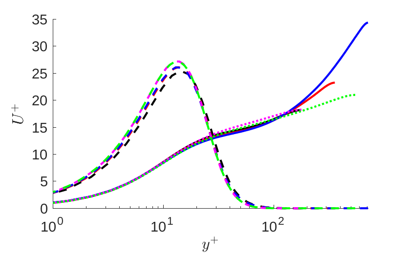
Figure 1: $U^{+}(y^{+})$ (black, red and blue solid lines for minimal channels at $Re_{\tau}=180,360$ and $720$ respectively, magenta and green dotted lines for LM15 channels at $Re_{\tau}=180$ and $550$ respectively). The primary streak profiles $A\tilde{u}^{0}_{n_{p}}(y;t_{p})$ (see expression (11) below) with $n_{p}=2$ or $\lambda_{z}^{p+}=84$ and $74$ for the minimal and large channels respectively, are shown using dashed lines and the corresponding colours with $A=10/\sqrt{Re_{\tau}}$ to highlight their similarity ($\tilde{u}^{0}_{n_{p}}(y;t_{p})$ is normalised to have the same amplitude as $U$ which scales with $\sqrt{Re_{\tau}}$ in viscous units). The primary streaks are all peaked at $y^{+}\approx 18$ consistent with the findings of Butler & Farrell (1993).

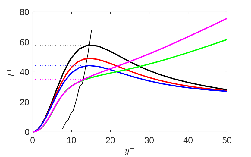
Figure 2: Eddy turnover time $t^{+}_{e}=q^{2}/\epsilon\,Re_{\tau}$ (black, red and blue lines for $Re_{\tau}=180,360$ and $720$ respectively, magenta and green lines for $Re^{LM15}_{\tau}=180$ and $550$ respectively) The location of the optimal streak as a function of the optimisation time is shown as a thin black curve for the minimal channel (the kinks in the curve are due to the discrete changes in optimal spanwise wavenumber of the streak). Chosen primary transient growth time horizons are marked with dotted lines. See Table 1 for numerical values of $t_{e}^{+}$ at the various $Re_{\tau}$.

2.2 Primary transient growth

We consider primary transient growth of the perturbations to the mean velocity profile $U(y)$ defined as $[{\tilde{u}},{\tilde{v}},{\tilde{w}}]=[u-U,v,w]$ and decomposed into streamwise and spanwise Fourier modes as follows:

$$[{\bm{\tilde{u}}}(x,y,z,t),{\tilde{p}}(x,y,z,t)]=\sum_{m,n}[\,\bm{\tilde{u}}^{m}_{n}(y,t),\tilde{p}^{m}_{n}(y,t)\,]\exp(im\alpha x+in\beta z)+c.c.$$ (5)

where $\alpha:=2\pi/L_{x}$ and $\beta:=2\pi/L_{z}$. The linearised Navier-Stokes equations around the mean $U(y)\hat{\mbox{\boldmath$x$}}$ for each $(m,n)$ are

$$\partial_{t}\bm{\tilde{u}}^{m}_{n}+im\alpha U\bm{\tilde{u}}^{m}_{n}+(\partial_{y}U)\tilde{v}^{m}_{n}\bm{\hat{x}}=-\bm{\nabla}\tilde{p}^{m}_{n}+\frac{1}{Re_{\tau}}\nabla^{2}\bm{\tilde{u}}^{m}_{n},\quad\bm{\nabla}\cdot\bm{\tilde{u}}^{m}_{n}=0$$ (6)

and can be treated separately. Due to the non-normality of the linear operator, the perturbations can experience transient growth in energy quantified by the (primary) gain

$$G_{p}(m,n,t_{p}):=\sup_{\bm{\tilde{u}}^{m}_{n}(y,0)}\frac{||\bm{\tilde{u}}^{m}_{n}(y,t_{p})||^{2}}{||\bm{\tilde{u}}^{m}_{n}(y,0)||^{2}}$$ (7)

where the energy norm is calculated by

$$E^{m}_{n}\vcentcolon=||\bm{\tilde{u}}^{m}_{n}||^{2}=\int_{-1}^{1}|\tilde{u}^{m}_{n}|^{2}+|\tilde{v}^{m}_{n}|^{2}+|\tilde{w}^{m}_{n}|^{2}\,dy.$$ (8)

The goal of the primary transient growth calculation is to identify the streamwise-independent streak field $\tilde{u}^{0}_{n_{p}}(y;t_{p})\exp(in_{p}\beta z)$ (with wavelength $\lambda_{z}^{p}:=2\pi/n_{p}\beta$) which achieves optimal energy growth at time $t_{p}$. This will then be used as the 2-dimensional streak field upon which to study secondary growth. Two issues require discussion: a) how to choose $t_{p}$ (which then specifies the streak spacing) and b) what amplitude to make the streaks for the secondary growth analysis.

2.3 Timescale for primary transient growth

Choosing the primary transient growth timescale $t_{p}$ presents a challenge as the global (over all $t_{p}$) optimal growth is achieved at a time much greater than characteristic timescale of turbulent fluctuations by perturbations with larger than observed spanwise spacing. Butler & Farrell (1993) realised that perturbations can only grow over the time limited by the eddy turnover time $t^{+}_{e}(y^{+})=q^{2}(y^{+})/\epsilon(y^{+})\,Re_{\tau}$ (the ratio of the characteristic turbulent velocity squared $q^{2}$ and dissipation rate $\epsilon$ at a given distance $y^{+}$ from the wall, given in viscous units) before being disrupted by turbulent fluctuations. Butler & Farrell (1993) suggested choosing $t^{+}_{p}=t^{+}_{e}(y^{+}_{*})$ where $y^{+}_{*}$ is the unique wall distance where the optimal streak is positioned given a growth time equal to the local eddy turnover time. While such restriction of the primary transient growth timescale was debated by Waleffe & Kim (1997) and Chernyshenko & Baig (2005), it provides a practical approach to obtain realistic streamwise streak profiles and will be used below. To calculate the eddy turnover time we use the following definitions:

$$q^{2}(y):=\frac{1}{TL_{z}L_{x}}\int_{T_{0}}^{T_{0}+T}\int_{0}^{L_{z}}\int_{0}^{L_{x}}\left[(u-U)^{2}+v^{2}+w^{2}\right]\,dx\,dz\,dt$$ (9)

$$\epsilon(y):=\frac{1}{TL_{z}L_{x}}\int_{T_{0}}^{T_{0}+T}\int_{0}^{L_{z}}\int_{0}^{L_{x}}|\mbox{\boldmath$\nabla$}({\bf u}-U\hat{\mbox{\boldmath$x$}})|^{2}\,dx\,dz\,dt.$$ (10)

Then, we compare the centre of the streak location (defined by maximum velocity) as a function of the streak optimisation time to the eddy turnover time $t^{+}_{e}$ as a function of the distance from the wall $y^{+}$, plotted using viscous units in Figure 2. The intersection points are at $t^{+}_{p}=57.6,\,48.6$ and $44.6$ for $Re_{\tau}=180,\,360$ and $720$ respectively in the minimal channel (giving a streak spacing of $\lambda_{z}^{p+}=84$) and at $t^{+}_{p}=35.0$ in the large channel for both $Re_{\tau}=180$ and $550$ (giving a streak spacing of $\lambda_{z}^{p+}=74$): see Table 1.

2.4 Amplitude for the primary streak

For the secondary transient growth calculation, the streamwise-independent base flow is defined as:

$${\cal U}(y,z)\hat{\mbox{\boldmath$x$}}:=U(y)\hat{\mbox{\boldmath$x$}}+\biggl{[}A{\tilde{u}}^{0}_{n_{p}}(y;t_{p})\exp(2\pi iz/\lambda_{z}^{p})+c.c\biggr{]}\hat{\mbox{\boldmath$x$}}$$ (11)

where $A$ is the primary streak amplitude with normalisation $||\tilde{u}^{0}_{n_{p}}(y;t_{p})||^{2}=||U||^{2}$ ( the ${\tilde{v}}^{0}_{n_{p}}$ component is not used). Without loss of generality, the streak field is chosen to be symmetric about $z=0$ and then ${\tilde{u}}^{0}_{n_{p}}(y;t_{p})$ is real. The amplitude $A$ was deduced directly from time-averaging our DNS data in the minimal channel or via the DNS data reported by LM15 for the larger channel. In the below, the mean amplitude, $\bar{A}$, and standard deviation $\sigma$ were collected for the minimal channel whereas only $\bar{A}$ was available for the large channel (see Table 1).

2.5 Secondary transient growth

Secondary transient growth perturbations are superimposed on the streak field ${\cal U}$ given in (11) so that ${\bm{\check{u}}}=[{\check{u}},{\check{v}},{\check{w}}]=[u-{\cal U},v,w]$ where ${\bm{\check{u}}}$ is assumed infinitesimally small. The secondary perturbation is decomposed into Fourier modes,

$$[{\bm{\check{u}}}(x,y,z,t),\check{p}(x,y,z,t)]=\sum_{m}[{\bm{\check{u}}}^{m}(y,z,t),\check{p}^{m}(y,z,t)]\exp{(im\alpha x)}$$ (12)

where

$$[{\bm{\check{u}}}^{m}(y,z,t),\check{p}^{m}(y,z,t)]=\sum^{N}_{n=-N}[{\bm{\check{u}}}^{m}_{n}(y,t),\check{p}^{m}_{n}(y,t)]\exp{(2\pi i(\mu+n)z/\lambda_{z}^{p})},$$ (13)

and $\mu\in[0,\tfrac{1}{2}]$ is a ‘modulation’ parameter . The secondary disturbance only has the same spanwise wavelength as the streak field when $\mu=0$ (no modulation) otherwise the spanwise wavelength of the secondary perturbation increases by a factor $1/\mu$ over that of the primary perturbation (e.g. the ‘subharmonic value of $\mu=\tfrac{1}{2}$ corresponds to the secondary having double the spanwise wavelength of the primary). In the periodic minimal box, formally we should consider all $\mu$ such that $1/\mu\in\mathbb{N}$ and $1/\mu$ is a factor of $n_{p}$ (note considering only $\mu\in(0,\tfrac{1}{2}]$ is sufficient due to the symmetries $\mu\rightarrow\mu\pm 1$ and $\mu\rightarrow-\mu$ under complex conjugation assuming $N$ is large enough).

In the linearised equations determining how ${\bm{\check{u}}}$ evolves, the Fourier modes in $x$ can be treated separately but the spanwise wavenumbers are coupled by the streak field adding new terms to the linearised equations (6):

$$\begin{split}\partial_{t}{\bm{\check{u}}}^{m}_{n}&+\overbrace{im\alpha[U{\bm{\check{u}}}^{m}_{n}+A{\tilde{u}}_{n_{p}}^{0}{\bm{\check{u}}}^{m}_{n-1}+A{\tilde{u}}_{n_{p}}^{0*}{\bm{\check{u}}}^{m}_{n+1}]}^{{\rm advection}}+\overbrace{(\partial_{y}U){\check{v}}^{m}_{n}\bm{\hat{x}}}^{{\rm lift-up}}\\ +&\underbrace{A\left[\partial_{y}{\tilde{u}}_{n_{p}}^{0}{\check{v}}^{m}_{n-1}+\partial_{y}{\tilde{u}}_{n_{p}}^{0*}{\check{v}}^{m}_{n+1}\right]\bm{\hat{x}}}_{{\rm extra\,\,lift-up}}+\underbrace{\tfrac{2\pi i}{\lambda_{z}^{p}}A\left[{\tilde{u}}_{n_{p}}^{0}{\check{w}}^{m}_{n-1}-{\tilde{u}}_{n_{p}}^{0*}{\check{w}}^{m}_{n+1}\right]\bm{\hat{x}}}_{{\rm push-over}}\\ &\hskip 28.45274pt=-\left(\begin{array}[]{c}im\alpha\\ \partial_{y}\\ 2\pi i(\mu+n)/\lambda_{z}^{p}\end{array}\right)\check{p}^{m}_{n}+\frac{1}{Re_{\tau}}\biggl{[}\partial_{y}^{2}-m^{2}\alpha^{2}-\frac{4\pi^{2}(\mu+n)^{2}}{(\lambda_{z}^{p})^{2}}\biggr{]}{\bm{\check{u}}}^{m}_{n}\end{split}$$ (14)

$$im\alpha{\check{u}}^{m}_{n}+\partial_{y}{\check{v}}^{m}_{n}+\frac{2\pi i(\mu+n)}{\lambda_{z}^{p}}{\check{w}}^{m}_{n}=0$$ (15)

We solve equations (14)-(15) for each value of $m$ (or equivalently wavelength $\lambda_{x}=2\pi/m\alpha=L_{x}/m$) separately while $2N_{z}+1$ spanwise modes are coupled using $n\in[-N_{z},N_{z}]$. The definition of the secondary gain is

$$G^{m}_{s}(t_{s};\lambda_{z}^{p+},A,Re_{\tau}):=\sup_{{\bm{\check{u}}}^{m}(y,0)}\frac{||{\bm{\check{u}}}^{m}(y,z,t_{s})||^{2}}{||{\bm{\check{u}}}^{m}(y,z,0)||^{2}}$$ (16)

and

$$G_{s}(t_{s};\lambda_{z}^{p+},A,Re_{\tau}):=\max_{m}G^{m}_{s}(t_{s};\lambda_{z}^{p+},A,Re_{\tau}).$$ (17)

is the optimal gain across the set of wavenumbers considered. We explore how this optimal gain changes as the primary streak amplitude $A$ is increased over the range of values observed in the simulations.

$N_{e}$		$\lambda_{x}^{+}=337$		$\lambda_{x}^{+}=674$
$T=0.2$  400		37.07 +  2.5 $\times 10^{-10}i$		6.38  -  1.1 $\times 10^{-9}i$
500		39.81		12,42 -  5.4 $\times 10^{-10}i$
600		40.61		19.80 -  2.2 $\times 10^{-2}i$
800		40.98		26.86 + 1.8 $\times 10^{-1}i$
1200		41.04		27.97 -  4.6 $\times 10^{-4}i$
1600		41.04		28.06 -  9.9 $\times 10^{-3}i$
$T=0.6$  400		7.79		1.99
500		8.56		2.01
600		8.76		2.02 + 1.7 $\times 10^{-5}i$
800		8.84		2.02 + 2.8 $\times 10^{-5}i$
1200		8.85		2.02 -  4.3 $\times 10^{-5}i$
1600		8.85		2.02 + 4.8 $\times 10^{-5}i$

Table 2: Convergence of growth factors with $N_{e}$, the number of eigenfunctions taken for the large channel and $Re_{\tau}=180$ using the narrow streak ($\lambda_{z}^{p+}=84$) primary flow at $T=0.2$ and $T=0.6$ with $\mu=0.001$ which mimicks the unmodulated case. Imaginary parts smaller than $10^{-10}$ are ignored. These results show that high wavenumbers and small times (top right) give problems whereas low wavenumbers and large times (bottom left) are easier to resolve.

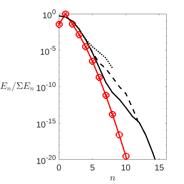
Figure 3: Energy distribution over spanwise wavenumbers $n$ for the optimal secondary transient growth mode at $\lambda_{x}=L_{x}$ and $Re_{\tau}=180$ in the minimal channel with primary streak $\lambda_{z}^{p+}=84$ and amplitude $\bar{A}$. Shown for $N_{z}=8,12$ and $16$ using black dotted, dashed and solid lines for the input modes (respectively), and red crosses, circles and a solid line (respectively) for the output modes. This figure indicates that even for $N_{z}=8$, there is a spectral drop off in energy of six orders of magnitude.

2.6 Numerical implementation

To perform the primary and secondary transient growth calculations, we follow the matrix-algebra approach described in Reddy & Henningson (1993) albeit with an adjustment to overcome a numerical issue. If ${\bf q}_{j}=(u_{j},v_{j},w_{j},p_{j})$ is the $j$th eigenfunction corresponding to the eigenvalue $\lambda_{j}$ and ordered by increasing damping rate $-Re(\lambda_{j})$, then Reddy & Henningson (1993) define the eigenvalue ‘overlap’ matrix as

$$C_{jk}:=\langle{\bf q}_{j},{\bf q}_{k}\rangle:=\int\int_{-1}^{1}\int u_{j}^{*}u_{k}+v_{j}^{*}v_{k}+w_{j}^{*}w_{k}\,\,dxdydz$$ (18)

where the inner product is that induced by the energy norm defined in (8), the integration is over a wavelength in $x$ and $z$, and ^∗ indicates complex conjugation. This matrix is diagonal if the eigenfunctions form an orthonormal set but, as is typical for shear flow problems, is dense here. It is, however, Hermitian and positive definite which means it has a Cholesky decomposition ${\bf C}={\bf F^{H}}{\bf F}$ where ${\bf F}$ is a real upper triangular matrix with positive entries along the diagonal and ${\bf F^{H}}:=({\bf F}^{*})^{T}$ is its Hermitian conjugate. Then the largest growth can be computed by squaring the largest singular value of ${\bf F}e^{t\mbox{\boldmath$\Lambda$}}{\bf F}^{-1}$ where $e^{t\mbox{\boldmath$\Lambda$}}$ is the diagonal matrix exponential with $e^{t\lambda_{j}}$ on the diagonal (see equation (30) in Reddy & Henningson (1993)). This approach, however, fails if ${\bf C}$ becomes non-positive definite through numerical errors as then the Cholesky decomposition aborts (Matlab actually advocates this as the best indicator of whether a matrix is positive definite or not). This sometimes happens for the secondary growth calculations when the matrices get too large (e.g. $O(10^{4})$ in dimension). An alternative approach employed is to handle the maximisation directly. If ${\bf u}=\sum_{j=1}^{N_{e}}a_{j}{\bf q}_{j}e^{t\lambda_{j}}$, then the energy growth is

$$G:=\max_{{\bf a}}\frac{{\bf a}^{\bf H}e^{t\mbox{\boldmath$\Lambda$}^{\bf H}}{\bf C}\,e^{t\mbox{\boldmath$\Lambda$}}{\bf a}}{{\bf a}^{\bf H}{\bf C}\,{\bf a}}$$ (19)

where ${\bf a}\in{\mathbb{C}}^{N_{e}}$ is the vector of coefficients which define the initial condition in terms of the eigenfunctions. The Euler-Lagrange equation which identifies (local and global) maximisers is

$$\sigma{\bf C}\,{\bf a}=e^{t\mbox{\boldmath$\Lambda$}^{\bf H}}{\bf C}\,e^{t\mbox{\boldmath$\Lambda$}}{\bf a}$$ (20)

which is a generalised eigenvalue problem where the largest $\sigma$ gives the global maximum. Again, there is a problem if ${\bf C}$ is not positive definite as then $\sigma$ fails to be real and positive. However, crucially the algorithm doesn’t suffer a hard failure but instead returns a number displaced off the positive real line. The relative size of the imaginary part to the real part gives some indication of the accuracy of the real part: see Table 2.

The symmetry in the wall-normal direction allows disturbances satisfying the symmetries

$$Z_{-}:(u,v,w,p)(x,y,z,t) \to(u,-v,w,p)(x,-y,z,t)$$

$$\&\quad Z_{+}:(u,v,w,p)(x,y,z,t) \to(-u,v,-w,-p)(x,-y,z,t)$$ (21)

to be considered separately. Discretisation of the linear operators corresponding to equations (6) and (14)-(15) produce matrices of size $2N_{y}$ and $2N_{y}(2N_{z}+1)$ respectively. For the primary transient growth calculation, $N_{e}=80$ eigenfunctions were used in the expansion which was tested by accurately reproducing the results in Butler & Farrell (1993) who use a modelled mean profile. Optimal streaks located near the wall were found to be the same for $Z_{-}$ and $Z_{+}$, and so the primary streak profile was chosen with $Z_{-}$ symmetry. No change in the optimal streaks were observed repeating the calculation with double the wall-normal resolution.

For the secondary transient growth calculation, a spanwise truncation of $N_{z}=8$ proved adequate typically giving a spectral drop off of over six orders of magnitude in the energy: see figure 6 which compares $N_{z}=8$, $12$ and $16$. The choice of appropriate $N_{e}$ is more delicate with increasing values needed for smaller $\lambda_{x}$ and short times: see Table 2. Typically $N_{e}=500-800$ was used as a compromise between accuracy and runtimes. In all cases, secondary perturbations with $Z_{-}$ symmetry yielded dominant transient growth values and are presented in this paper.

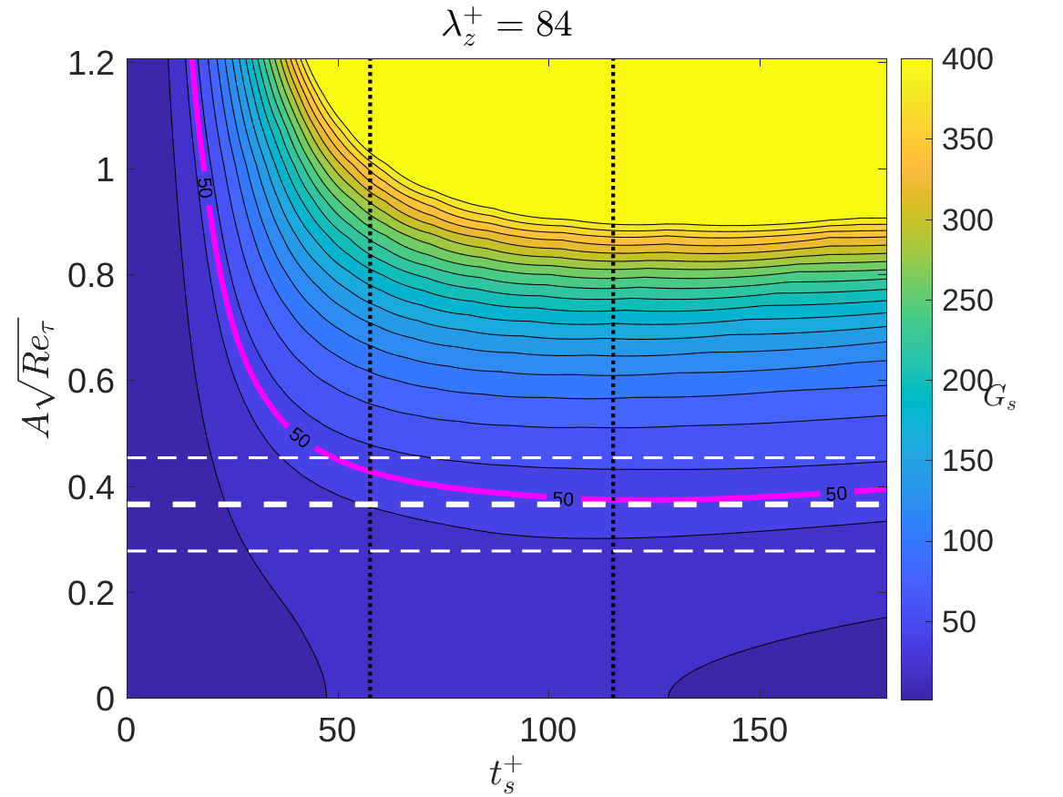
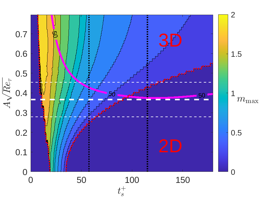
Figure 4: Left: secondary transient growth $G_{s}$ contour plots on the $(t_{s}^{+},A\sqrt{Re_{\tau}})$ plane at $Re_{\tau}=180$ for $\lambda^{+}_{z}=84$. Contour increments are 20. Right: corresponding optimal streamwise wavenumber $\alpha m_{max}=2\pi/\lambda_{x}^{+}$ over the set $m\in\{0,0.1,\ldots,2\}$ (there are 10 equally-spaced contour levels). A red dotted curve separates the regions where perturbations with $m=0$ (2D) and $m>0$ (3D) are optimal. In both plots, the white long dashed line shows $\bar{A}$ for the streaks with standard deviations are indicated by short dashed lines (both from DNS). Time horizons $t_{e}^{+}$ and $2t_{e}^{+}$ are marked with vertical black dotted lines and a magenta (left) or red (right) solid contour show the $G_{s}((\lambda_{x}^{+})_{\max})=50$ threshold.

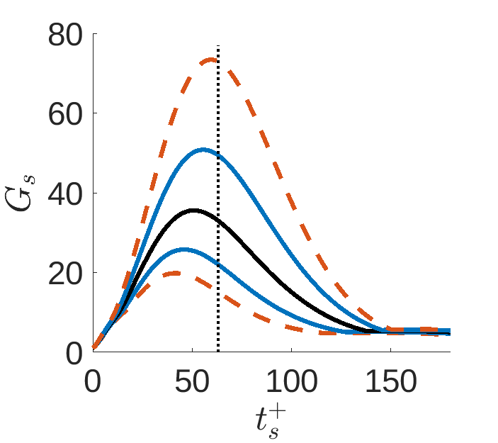
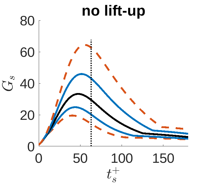
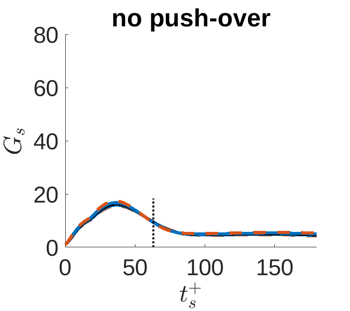
Figure 5: Secondary transient growth of perturbations with $\lambda_{x}=L_{x}$ ($m=1$) at $Re_{\tau}=180$ for $\lambda_{z}^{+}=84$. Energy gain $G_{s}(1,t_{s};A,180)$ is shown for different primary streak amplitudes $A=[\bar{A}_{84},\bar{A}_{84}\pm\sigma,\bar{A}_{84}\pm 2\sigma]$ (solid black, solid dark blue and dashed orange lines) and found a) with full linear mechanism b) excluding ‘lift-up’ c) excluding ‘push-over’. Dotted vertical lines show the $t_{s}=0.35$ time horizon.

3 Results

3.1 Two-Stage Optimisation

We first consider the minimal domain and $Re_{\tau}=180$ used by LM21. The approach taken here is to do two optimisations in sequence to estimate the energy growth possible in the flow over timescales consistent with the eddy turnover times near the wall. The first optimisation is used to define the streak field using linear transient growth analysis and the second optimisation then finds the optimal secondary growth on the primary streak field once it has been given an amplitude. The first has already been discussed with the result that a primary streak of spanwise spacing $\lambda_{z}^{p+}=84$ emerges using the approach advocated by Butler & Farrell (1993). The results of the secondary optimal gain $G_{s}(t_{s}^{+};84,A,Re_{\tau})$ contoured over the $(t_{s}^{+},A\sqrt{Re_{\tau}})$ plane is shown in Figure 4 with the associated optimising wavenumber index $m$ shown on the right. In their §6.3, LD21 discuss a threshold of $G_{s}=50$ for sustainable turbulence (although their figure 22 actually suggests the threshold is closer to 40 than 50) and so this contour is highlighted. The optimal growth possible at a representative time of $t_{e}^{+}=57.6$ is

$$G_{s}(t_{e}^{+};84,\bar{A}_{84},180)=38.4$$ (22)

with $m_{max}=0.7$ over the set $m\in\{0,0.1,\ldots,2\}$ ($\lambda_{x}^{+}=480$) rising to $\approx 55$ when the streak amplitude is $\bar{A}_{84}+\sigma$: here $\bar{A}_{\lambda_{z}^{+}}$ is defined as the observed mean amplitude for a streak of spanwise wavelength $\lambda_{z}^{+}$. This then gives growth levels consistent with the findings of LD21. It’s worth remarking that the secondary optimal energy gain is assessed here for disturbances with up to 5 times longer wavelength than fit in the original DNS (an advantage of this approach). Fig. 4 also shows that this growth is quite insensitive to the optimisation time $t_{s}$: the $G_{s}=50$ contour sits in the $\bar{A}$ range $[\bar{A}_{84},\bar{A}_{84}+\sigma]$ from about $t_{s}^{+}\approx 50$ up to well over 150. The optimal wavenumber $m_{max}$, however, does monotonically decrease from $0.7$ down to 0 as $t_{s}$ increases with the 3D-to-2D transition occurring near $t_{s}^{+}=100$.

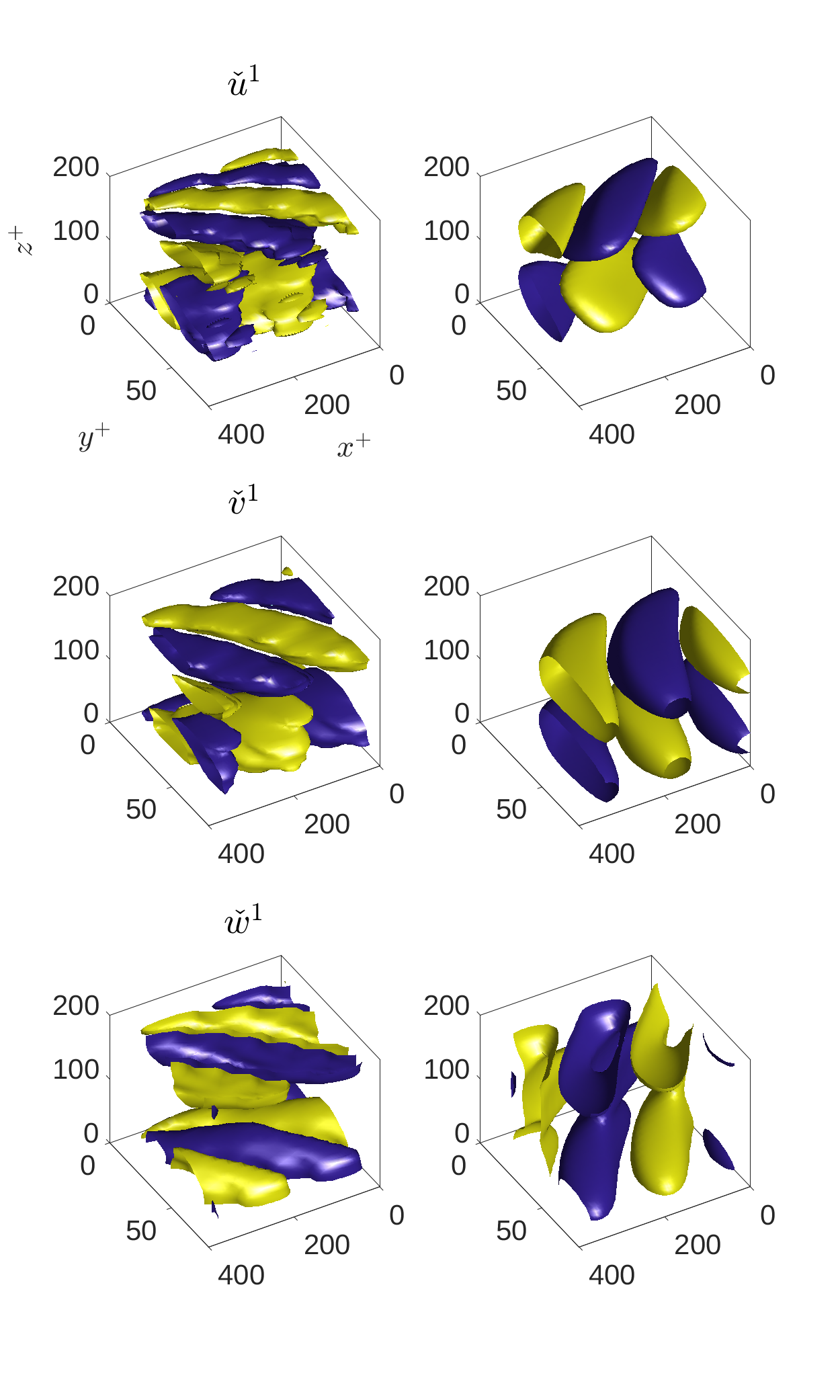
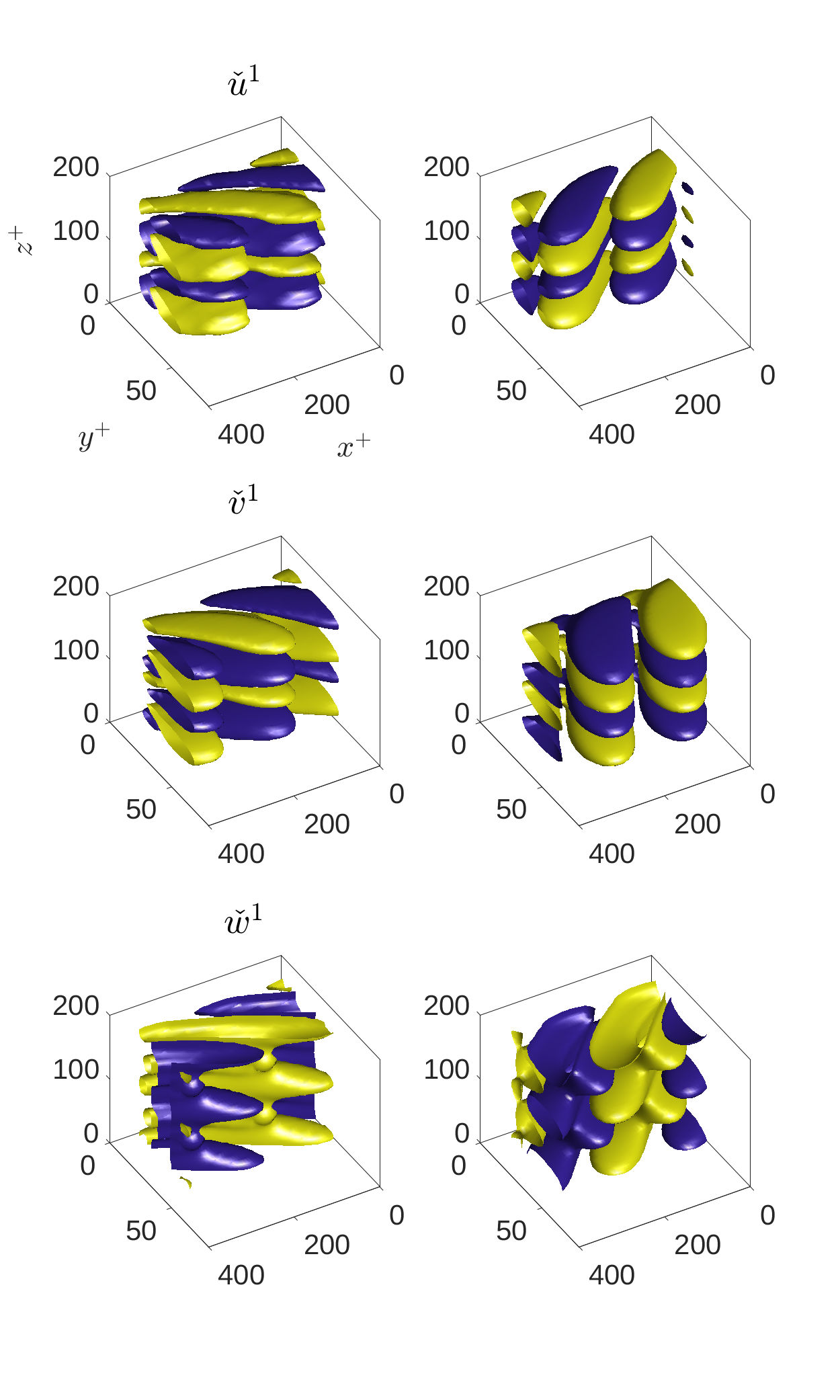
Figure 6: Optimal secondary transient growth modes with $\lambda_{x}^{+}=337$ at $Re_{\tau}=180$, primary streak amplitude $A=\bar{A}$ and $t_{e}$. Shown for small channel streaks with $\lambda^{+}_{z}=168$ (left two columns) and $\lambda^{+}_{z}=84$ (right two columns). Optimal input velocities are shown on the left column and optimal output velocities are shown on the right column of the two-column structure. The blue and yellow isosurfaces show $\pm 0.2$ of the maximum of each velocity component. The key takeaway is that there are similar structures for short and long streaks, with the structures reaching further from the wall for longer streaks.

A key finding from LD21 (see their §6.4) is that the ‘lift-up’ mechanism is not important for the growth they observe but the ‘push-over’ and Orr mechanisms are. To test this in our calculations, we consider the growth for the specific case of $m=1$ ($\lambda_{x}^{+}=337$) which just fits in the minimal channel and so was considered by LD21, and suppress either the lift-up or push-over mechanisms in turn: see Fig. 5. With both present, the growth can range from 20 to 74 as the streak amplitude increases from $\bar{A}_{84}-2\sigma$ to $\bar{A}_{84}+2\sigma$. The maximum growth at $A=\bar{A}_{84}$ is observed at $t^{+}_{s}=50$ which is very close to the eddy turnover time $t^{+}_{e}=57.6$ chosen in Section 2.3 suggesting that both primary and secondary transient growth processes might evolve over similar timescales. These results are in good agreement with LD21 where energy gains of the frozen-in-time-streak field reach $\mathcal{O}(100)$ at $T^{LD}_{max}=0.35$ or in viscous units $63$ (see discussion surrounding their Figure 9). Further agreement with LD21 is found when considering the effect of lift-up and push-over mechanisms on the optimal gain values. While excluding the lift-up mechanism has only a minor decreasing effect on the secondary transient growth, excluding the push-over mechanism causes the maximum optimal gain to collapse to $G_{s}\approx 16$ independent of the streak amplitude and shifting the optimal timescale back to $t_{s}=0.20$. We thus also find that the ‘push-over’ mechanism is essential to obtain sufficient levels of transient growth needed to sustain turbulence whereas the lift-up mechanism is not.

Figure 6 illustrates a typical secondary optimal example at streamwise wavenumber $m=1$ ($\lambda_{x}^{+}=337$) for the streak amplitude $A=\bar{A}_{84}$ (the optimal is shown in the third column and the final evolved state in the fourth column from left). Similar to the optimal modes found around the laminar velocity profile with a spanwise streak (Cossu et al., 2007), the optimal modes are tilted upstream at the start of the process (flow is from right to left) and are then tilted downstream at the time of the maximum energy gain, with the wall-normal velocity component almost perpendicular to the wall. This indicates that the Orr mechanism is operative.

There is, however, one inconsistency with the findings of LD21: their velocity snapshots - e.g. their figures 2 and 3 - show a dominant single streak which corresponds to $n_{p}=1$ or $\lambda_{z}^{p+}=168$ rather than the $n_{p}=2$ or $\lambda_{z}^{p+}=84$ primary optimal found here. Re-examining the DNS shows evidence of $\lambda_{z}^{p+}=84$ streaks but they are clearly dominated by the $\lambda_{z}^{p+}=168$ streaks - see Fig. 7. The DNS indicates that the $\lambda_{z}^{p+}=168$ streaks have a mean amplitude of $0.92/\sqrt{Re_{\tau}}$ compared to $0.37/\sqrt{Re_{\tau}}$ for the $\lambda_{z}^{p+}=84$ with smaller spanwise wavelength streaks having yet smaller amplitudes still. This suggests that the two-stage optimisation procedure described above isn’t quite correct. A small adjustment in it is to take the $n_{p}=1$ optimal streak as the primary i.e. $\lambda_{z}^{p+}=168$ and rerun the secondary optimisation to see what the growth is then.

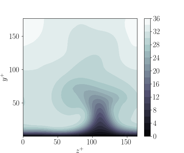
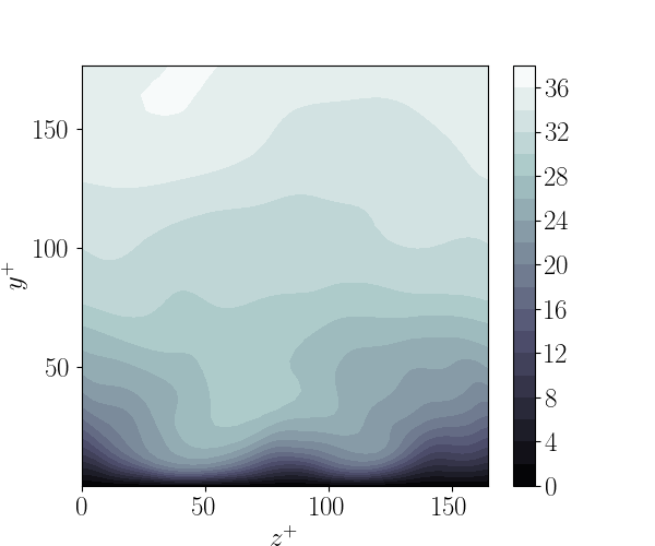
Figure 7: Sample snapshots of the $x$-averaged velocity field $U^{+}(y^{+},z^{+})$ from a $Re_{\tau}=180$ simulation in the minimal channel of LD21. Left: streaks with $\lambda^{p+}_{z}=168$ ($n_{p}=1$) and Right: streaks with $\lambda^{p+}_{z}=84$ ($n_{p}=2$). These figures show that both primary optimal and dominant streaks are visible at different times in the simulations.

3.2 A Modified Two-Stage Optimisation

The two-stage optimisation procedure above identified the optimal primary streak which emerges with the largest growth at the local eddy-turnover time by maximising growth over all initial disturbances of a given spanwise wavelength and then over all spanwise wavelengths $\lambda_{z}^{+}$. Here, given the differences in the observed mean streak amplitudes, we restrict the optimisation to all initial disturbances with $\lambda_{z}^{p+}=168$. The objective is then to compare the secondary growth possible on this less optimal but larger amplitude streak with that available off the optimal $\lambda_{z}^{p+}=84$ streak.

Figure 8 shows the secondary growth for $\lambda_{z}^{p+}=168$ over the $(t_{s}^{+},A\sqrt{Re_{\tau}})$ plane. The relevant turnover time $t_{e}^{+}$ for $\lambda_{z}^{p+}=168$ - the leftmost dotted vertical black line - is essentially the same as for $\lambda_{z}^{p+}=84$. This is because the thin black line in Figure 2 which represents the $y^{+}=y^{+}(t^{+})$ relationship between the maximal streak growth over $t^{+}$ and its peak magnitude location at $y^{+}$ only moves very slightly near its intersection with $t_{e}^{+}(y^{+})$ when the maximization is restricted to just $\lambda_{z}^{p+}=168$ disturbances. The growth possible at $A=\bar{A}_{84}$ is lower than that on the $\lambda_{z}^{p+}=84$ streak,

$$G_{s}(t_{e}^{+};168,\bar{A}_{84},180)\approx 24.6\,<\,G_{s}(t_{e}^{+};84,\bar{A}_{84},180)$$ (23)

with $m_{max}=0.5$ over $m\in\{0,0.1,\ldots,2\}$ as has to be the case. However, at $A=\bar{A}_{168}$ much higher growth is possible, in particular,

$$G_{s}(t_{e}^{+};168,\bar{A}_{168},180)\approx 91.8$$ (24)

with $m_{max}=1$ over $m\in\{0,0.1,\ldots,2\}$. Figure 8 (right) emphasizes the extra growth possible for the wider streak because of its larger amplitude as a function of $t^{+}_{s}$. It might now appear that there is too much growth available to be consistent with LD21 but this is because these estimates are maximums rather than expected values given generic, non-optimal initial secondary perturbations. An recent interesting study making this precisely point is Frame & Towne (2023).

The conclusion of this and the previous sections is then that a two-stage optimisation procedure is able to capture the levels of growth found by LD21 in their DNS and the importance/unimportance of the push-over/lift-up mechanism in this. The slight wrinkle is that the spanwise spacing of the primary streak predicted by the procedure isn’t quite the dominant one seen in the DNS. However, when the optimal streak of that spanwise spacing is swapped in, the maximum growths predicted are entirely consistent with the growths seen by LD21. The questions now are a) how do the possible growths vary with $Re_{\tau}$? and b) how do things change with a larger channel? In the latter, for example, it is unlikely that the most energetic streak will be that with the largest spacing which fits into a larger domain.

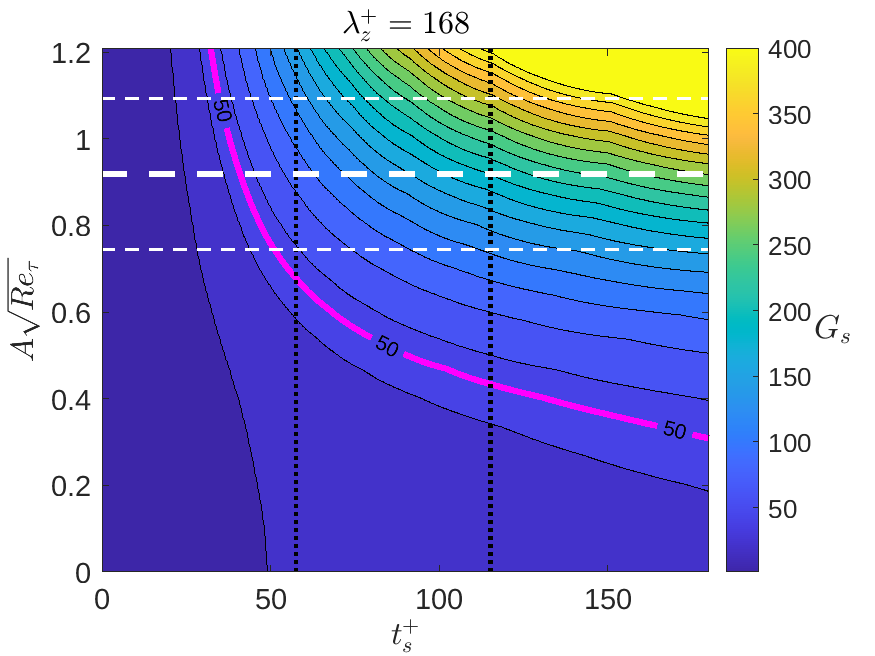
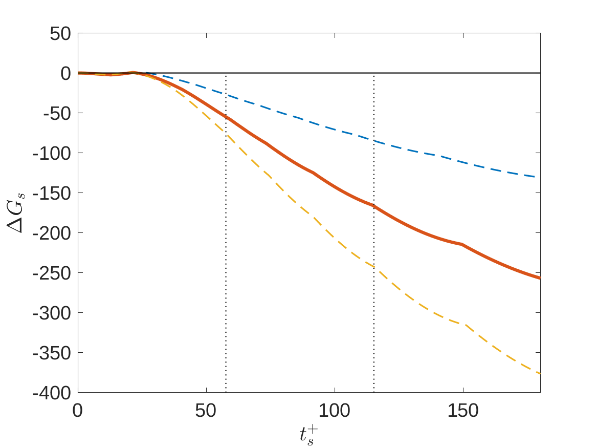
Figure 8: Left: secondary transient growth $G_{s}(t_{s}^{+};168,A,Re_{\tau}=180)$ contour plots over the $(t_{s}^{+},A\sqrt{Re_{\tau}})$ plane. Contour increments are 20. Right: a comparison of the growth achieved at $\lambda_{z}^{+}=84$ and $168$ at their respective average amplitudes: $\Delta G_{s}=G_{s}(t_{e}^{+},84,A_{84},180)-G_{s}(t_{e}^{+},168,A_{168},180)$ where $A_{\lambda_{z}^{+}}=\bar{A}_{\lambda_{z}^{+}}$ (red curve) or $\bar{A}_{\lambda_{z}^{+}}\pm\sigma$ (⁺yellow & _-blue dashed curves). This plot shows that the extra amplitude of the $\lambda_{z}^{+}=168$ streaks creates more secondary growth than the lower amplitude $\lambda_{z}^{+}=84$ streaks.

3.3 Higher $Re_{\tau}$

To explore higher $Re_{\tau}$ without changing the domain, the two-stage optimisation procedure was repeated at $Re_{\tau}=360$ and $Re_{\tau}=720$ in the minimal channel. The optimal primary streak remains $\lambda_{z}^{p+}=84$ and the corresponding zoomed-in contour plots of the optimal transient growth on the $(t_{s}^{+},A\sqrt{Re_{\tau}})$ plane are shown in Figure 9 for relevant primary streak amplitudes observed in the simulations. The plot remains largely unchanged when $Re_{\tau}$ is increased. The mean streak amplitude observed in the simulations is decreasing but the growth actually increases slightly,

$$G_{s}(t_{e}^{+};84,\bar{A}_{84},360)\approx 36.1$$ (25)

and

$$G_{s}(t_{e}^{+};84,\bar{A}_{84},720)\approx 38.4$$ (26)

where, for both, $m_{max}=0.9$ over $m\in\{0,0.1,\ldots,2\}$. The $G_{s}=50$ contour remains within the standard deviation of the mean streak amplitude at $t^{+}_{e}$. The main change is that the contours become steeper for $Re_{\tau}=720$ which results in the contour $G_{s}=55$ reaching the minimum amplitude $\bar{A}\sqrt{Re_{\tau}}$ near $2t^{+}_{e}$ time instead of the $G_{s}=50$ contour for the two lower $Re_{\tau}$. Rather than repeating this process for the $\lambda_{z}^{p+}=168$ streak, we move out of the minimal channel to consider more streak spacings.

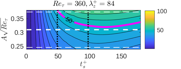
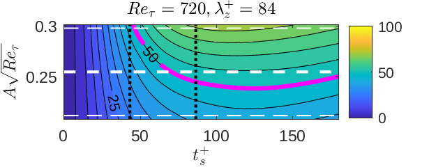
Figure 9: $G_{s}((\lambda_{x}^{+})_{\max})$ zoomed in to the relevant amplitudes at $Re_{\tau}=360$ (left) and $Re_{\tau}=720$ (right) for the optimal streak $\lambda_{z}^{p+}=84$. Time horizons $t_{e}^{+}$ and $2t_{e}^{+}$ are marked with vertical black dotted lines. Horizontal white dashed lines show $\bar{A}\sqrt{Re_{\tau}}$ and $\left(\bar{A}\pm\sigma\right)\sqrt{Re_{\tau}}$. Red solid contour shows $G_{s}((\lambda_{x}^{+})_{\max})=50$ threshold. Contour levels have $\Delta G=5$.

3.4 Larger Geometry

Here, we use the DNS data from the larger channel studied in LM15 (see Table 1 for details) to investigate the presence of larger lengthscales in the two-stage optimisation procedure (e.g. the larger channel is over an order of magnitude wider). The mean profiles shown in Figure 1(top) are fairly similar for $Re_{\tau}=180$ (black solid line versus magenta dotted line) but, as expected, start to deviate in the interior for higher $Re_{\tau}$: compare the profile at $Re_{\tau}=550$ for the larger channel (green dotted line) with the minimal channel profile at $Re_{\tau}=720$ (blue solid line). The eddy turnover time functions $t_{e}^{+}(y^{+})$ also behave differently at large $y^{+}$. However, the key area of the curve at lower $y^{+}$ intersects with the optimal streak function at roughly the same streak position albeit at a reduced turnover time $t_{e}^{+}(y^{+}_{*})$ of 35 for $Re_{\tau}=180$ and 37 for $Re_{\tau}=550$. As a consequence, the resulting optimal primary streaks are very similar in structure (upper plot in figure 1) and spanwise wavelength: $\lambda_{z}^{p+}=74$ in the larger channel for both $Re_{\tau}=180$ and 550 as opposed to $84$ in the minimal channel. The conclusion is then that the primary optimal streaks are truly near-wall structures which have already converged in form at $Re_{\tau}=180$ in a large channel.

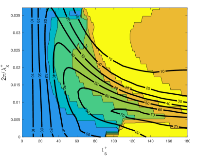
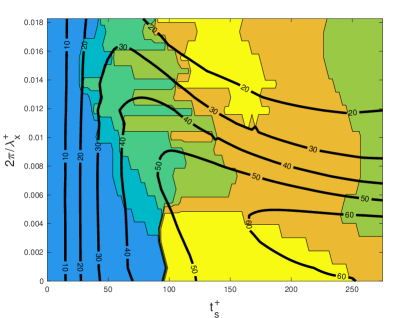
Figure 10: A plot of maximum growth as a function of $t_{s}^{+}$ and streamwise wavenumber $2\pi/\lambda_{x}^{+}$ and optimised over spanwise modulation $\mu\in\{0,0.1,0.2,0.25,0.3333,0.5\}$ for $Re=180$ and $\lambda_{z}^{p+}=84$ (left) and $Re=550$ and $\lambda_{z}^{p+}=74$ (right), both using the mean streak amplitude from LM15. Black contour lines show maximum growth levels and the 6 colours indicate the maximising $\mu$: $\mu=0$ (blue), $0.1$ (light blue), $0.2$ (emerald), $0.25$ (green), $0.3333$ (dark orange), $0.5$ (yellow) in both plots. Values used for $N_{e}$ ranged from 600 to 1200. These plots indicate that a modulated secondary transient is preferred if $t_{s}^{+}$ is large enough (with the spanwise modulation wavelength generally decreasing with increasing $t_{s}^{+}$) and the growth is insensitive to $2\pi/\lambda_{x}^{+}$ at low $t_{s}^{+}$.

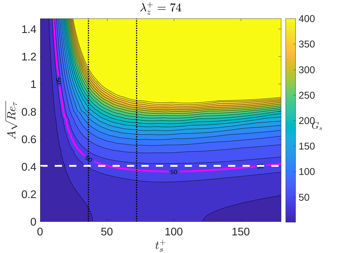
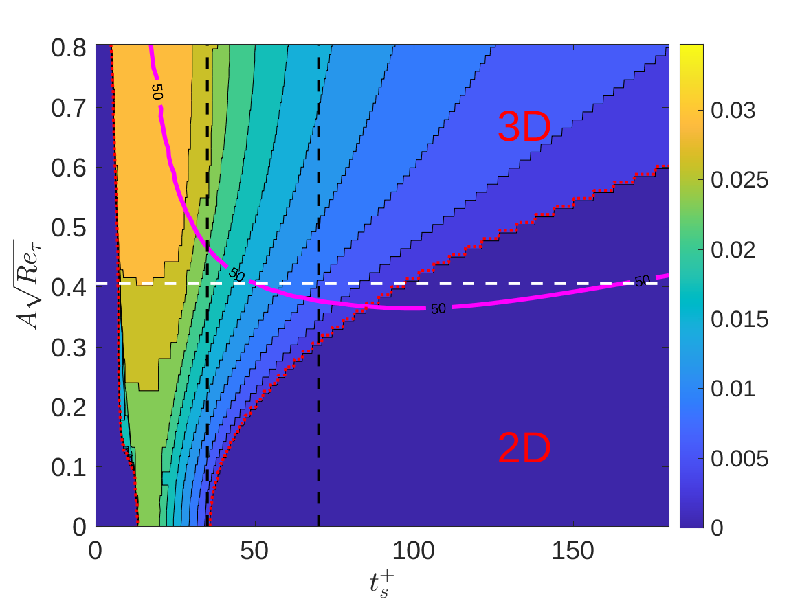
Figure 11: Left: Secondary transient growth $G_{s}$ contour plot over the $(t_{s}^{+},A\sqrt{Re_{\tau}})$ plane at $Re_{\tau}=180$ for the LM15 channel and $\lambda^{+}_{z}=74$. The white dashed line shows $\bar{A}$ for the primary streaks. Time horizons $t_{e}^{+}$ and $2t_{e}^{+}$ are marked with vertical black dotted lines. The magenta solid contour shows $G_{s}((\lambda_{x}^{+})_{max})=50$. Contour increments are 20. Right: corresponding optimal streamwise wavenumber $2\pi/(\lambda_{x}^{+})_{\max}$: 10 contours used. The red dotted curve separates the regions where optimal perturbations are 2D from those which are 3D.

The secondary growth computation is more involved in the larger LM15 channel because secondary perturbations of much larger spanwise wavelength than the primary streaks are possible. Operationally, this means the secondary growth search must be extended to sweep over possible modulation parameters $\mu\in[0,\tfrac{1}{2}]$ (see (13)). To explore whether such modulations are important, the maximum secondary growth at both $Re_{\tau}=180$ and 550 is computed on the optimal primary streak (assumed to have the observed mean amplitude): shown as contours over $(t_{s}^{+},2\pi/\lambda_{x}^{+})$ plane in figure 10. The colours used indicate the modulational parameter which gives the maximum at a given $(t_{s}^{+},2\pi/\lambda_{x}^{+})$ point. Since the $\mu=0$ (no modulation) blue colour is prominent for $t_{s}^{+}\lesssim t_{e}^{+}=35$, the conclusion is that modulational effects are not important here. However for longer times, modulated secondary optimals clearly become preferred which offers an intriguing mechanism for energy to transfer upscale. For the narrative here, however, we no longer need to consider modulational effects.

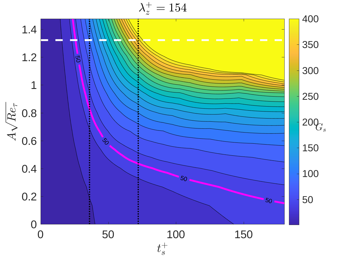
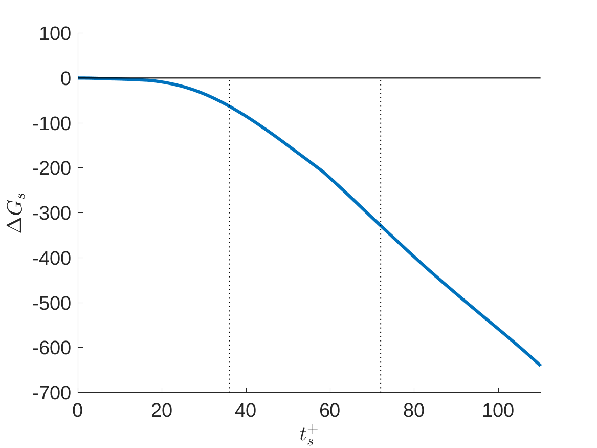
Figure 12: Left: Secondary transient growth $G_{s}$ contour plot over the $(t_{s}^{+},A\sqrt{Re_{\tau}})$ plane at $Re_{\tau}=180$ for the LM15 channel and $\lambda^{p+}_{z}=154$. Time horizons $t_{e}^{+}$ and $2t_{e}^{+}$ are marked with vertical black dotted lines. The magenta solid contour shows $G_{s}((\lambda_{x}^{+})_{\max})=50$. Takeaways: short and long channel similarity, necessity of 3D structures to support secondary growth. 10 equally spaced contours. Right: secondary transient growth difference between the wide and narrow streaks at their respective average amplitudes: $\Delta G_{s}=G_{s}(t_{e}^{+},74,\bar{A}_{74},180)-G_{s}(t_{e}^{+},154,\bar{A}_{154},180)$. Takeaway: long streaks have dominant secondary transient growth over short streaks.

Another interesting observation from figure 10 for $t_{s}^{+}\lesssim t_{e}^{+}=35$ is that the optimal growth rate contours are nearly parallel with the streamwise wavenumber axis. This implies that the maximum over streamwise wavenumbers is almost flat - i.e. the growth only changes slowly with $\lambda_{x}^{+}$ - and it is tempting to speculate would be become increasing close to being flat as $Re_{\tau}\rightarrow\infty$. This would indicate a broadband response of secondary scales growing together on a primary streak. As a result of this phenomenon, it is both difficult and less meaningful to identify the optimal secondary streamwise wavelength in what follows so we only do it for our initial calculation (figure 11).

Taking $\mu=0$ henceforth, figure 11 shows the optimal secondary growth and corresponding wavenumber over the $(t_{s}^{+},A\sqrt{Re_{\tau}})$ plane with $Re_{\tau}=180$ for the optimal streak $\lambda_{z}^{p+}=74$. The contour plots look very similar to the minimal channel results in figure 4 with comparable growth possible, e.g.

$$G_{s}(t_{e}^{+};74,\bar{A}_{74},180)\approx 40.2$$ (27)

where $m_{max}=0.9$ over $m\in\{0,1,\ldots,25\}$ (chosen so the smallest streamwise wavelength $\lambda_{x}=8\pi/25$ is approximately that used in the minimal channel $1.87/2$).

Again the streak of largest observed amplitude, $\lambda_{z}^{p+}=154$, is roughly twice the spacing of the optimal primary streak. The secondary growth associated with this larger streak is shown in figure 12 which also contains a comparison with that possible off the optimal primary but smaller-amplitude streak $\lambda_{z}^{p+}=74$. These plots and corresponding optimals (not shown) are also very similar to the minimal channel results in figure 8 with the estimate

$$G_{s}(t_{e}^{+};154,\bar{A}_{154},180)\approx 97.5$$ (28)

slightly enhanced from the 91.8 of (24). It seems at least at $Re_{\tau}=180$, working in a larger domain does not change the conclusions drawn at the end of §3.2.

At $Re_{\tau}=550$ in the large channel, the primary optimal streak has again $\lambda_{z}^{p+}=74$ whereas the streak of largest mean amplitude is $\lambda_{z}^{p+}=136$ - see Figure 13 for streak energy distribution between streak wavelengths $\lambda_{z}^{p+}$ at $Re_{\tau}=550$.

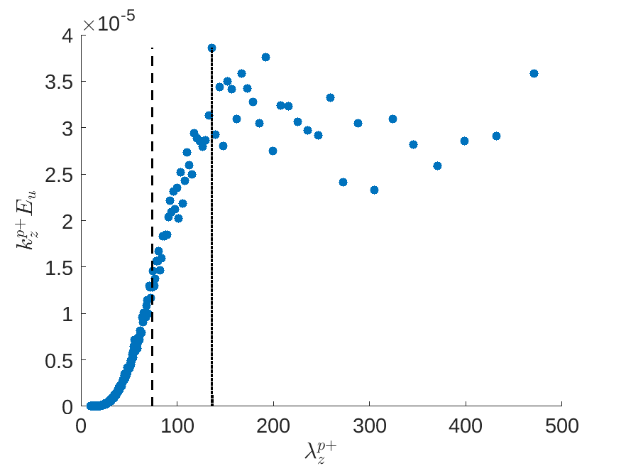
Figure 13: Streak energy $E_{u}$ premultiplied by $k_{z}^{p+}=2\pi/\lambda_{z}^{p+}$ against streak wavelength $\lambda_{z}^{p+}$ in LM15 simulations shown for $Re_{\tau}=550$. The streak energy was integrated up to $y^{+}\approx 18$ to focus on the near-wall structures only. Vertical dashed line shows the optimal streak with $\lambda_{z}^{p+}=74$ and vertical dotted line shows the most energetic streak with $\lambda_{z}^{p+}=136$.

Zoomed-in plots of the secondary growth possible over time and streak amplitude for these are shown in figure 14. The key secondary growth estimators are

$$G_{s}(t_{e}^{+};74,\bar{A}_{74},550)\approx 23.4$$ (29)

and

$$G_{s}(t_{e}^{+};136,\bar{A}_{136},550)\approx 28.4$$ (30)

which are noticeably reduced from $Re_{\tau}=180$ and interestingly much more similar to each other. Assuming this two-stage optimisation is capturing the correct behaviour, this indicates that the required energy growth needed to sustain turbulence is a decreasing function of $Re_{\tau}$.

The fact that the maximum secondary growth for the two primary streaks is much closer at $Re_{\tau}=550$ than $Re_{\tau}=180$ can partially be explained by the convergence of their spanwise wavelengths. But it is more likely that the growth is becoming insensitive to the exact spanwise spacing. Taken together with the emerging insensitivity of the secondary growth to streamwise wavelengths shown in figure 10, this reflects the familiar phenomenon of more and more degrees of freedom becoming active as $Re_{\tau}$ increases.

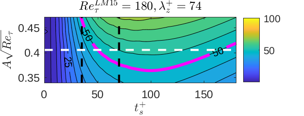
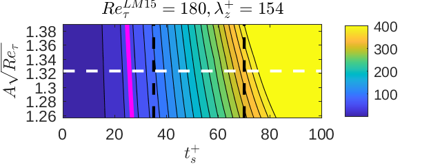
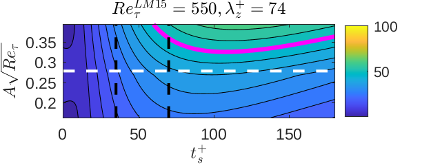
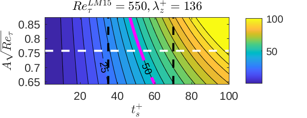
Figure 14: Secondary transient growth for large LM15 channels. Contour levels every $\Delta G=5$ except for top right where contour levels are every $\Delta G=20$. The top plots reproduce the results of figures 11 and 12 in this modified format to aid comparison. The magenta curve is the $G_{s}=50$ contour.

4 Conclusions

In this study we have attempted to dissect the recent observation made in Lozano-Duran et al. (2021) (LD21) that viable streamwise-averaged flows in minimal channels achieve a threshold level of rapid transient growth. By examining a relatively simple two-stage model of primary transient streak growth on a spanwise-invariant mean and then secondary transient growth on the now presumed frozen streaky primary flow, energy gain levels, timescales and the importance of the ‘push-over’ mechanism were all found to be consistent with the results of LD21 at $Re_{\tau}=180$ in their minimal channel. Repeating our analysis for a larger channel using the database of Lee & Moser (2015) (LM15) shows that the findings at $Re_{\tau}=180$ are essentially unchanged: the primary optimal streak has basically the same structure albeit with a slightly modified spanwise spacing and the secondary growth possible is very similar. As in the minimal channel, the DNS data from LM15 suggests that in fact, the most energetic streak has a spanwise spacing roughly twice that of the predicted optimal primary streak and with its higher amplitude, much more secondary energy growth is possible. At $Re_{\tau}=550$, however, this most energetic streak spacing is found to move closer to the optimal primary, which is unchanged from $Re_{\tau}=180$, and their secondary growth properties both decrease and become much more comparable. Our conclusion is then that the threshold transient growth for turbulence sustainability decreases going from $Re_{\tau}=180$ to $Re_{\tau}=550$ but remains driven by the same near-wall streak field.

The main benefit of our modelling approach is its interpretability and the ability to look at larger domains and higher $Re_{\tau}$ relatively cheaply as done here. A DNS needs to be run to estimate the mean profile $U(y)$ (although a parameterised profile would probably suffice), the eddy turnover function $t_{e}^{+}(y^{+})$ and the streak amplitudes. After that, the rest of the calculations are based on the spectral properties of appropriate linear operators. In particular, onerous time-dependent optimisation calculations are avoided. There is no denying, however, that the two-stage optimisation procedure explored here is perhaps the simplest model which could be imagined relevant to LD21 and is admittedly heuristic. The primary streaks are imagined to grow over a time $t_{e}^{+}$ and then artificially ‘frozen’ so a secondary transient growth calculation can be performed typically over another (streak) eddy turnover time $t_{e}^{+}$. This has the advantage of involving only two linear computations performed here using standard matrix algebra albeit with the necessity of inserting the observed amplitude for the streak halfway through the process. A more realistic calculation would be to do a full optimisation problem where the secondary growth is optimised over all possible streak structures again frozen in time. A further step closer to reality would be to allow the streaks to evolve and then even allowing the growing secondary perturbations to influence the streak evolution. These problems are, of course, much more intensive computations seeking to get ever closer to the underlying simulations but at the same time run the risk of losing interpretability as they complexify. Nevertheless, there is no doubt a more joined-up optimisation procedure would be worth pursuing. The recent work computing growth for finite amplitude disturbances (e.g. Kerswell, 2018) points the way forward for examining the growth possible from the mean flow $U(y)\hat{\mbox{\boldmath$x$}}$ in which the initial streak field $[U(y,z,0)-U(y)]\hat{\mbox{\boldmath$x$}}$ is constrained to have a certain amplitude but is otherwise free to be optimised. It would surely be fascinating to see if the optimal which emerges from this one-step optimisation would resemble that assumed in our two-stage procedure.

Another interesting direction for development is trying to estimate expected rather than maximum growth values. LD21 test an ensemble of streamwise-averaged DNS velocity fields for energy growth capability and folding in more of the properties of this into the secondary growth problem would clearly be valuable. A recent study by Frame & Towne (2023) has started to consider how the distribution of fluctuations available to initiate growth can influence the expected growth later. Here, the more relevant calculation would be to study what the expected secondary growth characteristics are on the observed primary streak distribution.

Mechanistically, Lozano-Duran et al. (2021) speculate that both the Orr and ‘push-over’ effects are needed for sustaining turbulence in minimal channels. However, these two processes act over very different timescales: while the Orr mechanism acts on the fast advective timescale ( $\mathcal{O}(0.15h/u_{\tau})$ found by Jiménez (2015) in channel flow), ‘push-over’ acts on the slow viscous timescale. It remains unknown how these two processes synergise in a linear calculation to create optimal growth that cannot be achieved by only one of the two (the ability for one to pump prime the other is clear from nonlinear calculations, e.g. see the appendix B in Kerswell et al. (2014)). A study in the spirit of Jiao et al. (2021), who recently looked at the synergy between the ‘lift-up’ and Orr processes, seems called for although the base flow has to be spanwise-varying to activate ‘push-over’ which will significantly complicate matters.

Finally, we remark that the observation of Lozano-Duran et al. (2021) presents a very plausible correction to Malkus’s (1956) assertion that turbulent (spanwise-averaged) mean profiles are marginally stable. Rather than a long term (asymptotic) spectral condition, the mean profile may actually satisfy a threshold for rapid short term growth instead. The work presented here is consistent with the engine for this growth - the primary streak field - being in the near-wall region and has found that the growth threshold decreases with $Re_{\tau}$. Future DNS work will be needed to corroborate these findings and then the challenge will be to exploit them.

[Acknowledgement]The authors are very grateful to Myoungkyu Lee for generously sharing data from his large channel simulations (Lee & Moser 2015).

[Funding]VKM acknowledges financial support from EPSRC through a PhD studentship. [Declaration of interests] The authors report no conflict of interest.

References

- del Alamo & Jimenez (2006) del Alamo, J. C. & Jimenez, J. 2006 Linear energy amplification in turbulent channels. J. Fluid Mech. 559, 205–213.
- Andersson et al. (2001) Andersson, Paul, Brandt, Luca, Bottaro, Alessandro & Henningson, Dan S. 2001 On the breakdown of boundary layer streaks. Journal of Fluid Mechanics 428, 29–60.
- Burns et al. (2020) Burns, Keaton J., Vasil, Geoffrey M., Oishi, Jeffrey S., Lecoanet, Daniel & Brown, Benjamin P. 2020 Dedalus: A flexible framework for numerical simulations with spectral methods. Physical Review Research 2 (2), 023068, arXiv: 1905.10388.
- Butler & Farrell (1993) Butler, K. M. & Farrell, B. F. 1993 Optimal perturbations and streak spacing in wall-bounded turbulent shear flow. Phys. Fluids 5, 774.
- Chernyshenko & Baig (2005) Chernyshenko, S. I. & Baig, M. F. 2005 The mechanism of streak formation in near-wall turbulence. Journal of Fluid Mechanics 544, 99–131.
- Cossu et al. (2007) Cossu, Carlo, Chevalier, Mattias & Henningson, Dan S. 2007 Optimal secondary energy growth in a plane channel flow. Physics of Fluids 19 (5), 058107, arXiv: https://doi.org/10.1063/1.2736678.
- Cossu et al. (2009) Cossu, C., Pujals, G. & Depardon, S. 2009 Optimal transient growth and very large structures in turbulent boundary layers. J. Fluid Mech. 619, 79.
- Farrell (1988) Farrell, Brian F. 1988 Optimal excitation of perturbations in viscous shear flow. The Physics of Fluids 31 (8), 2093–2102.
- Farrell & Ioannou (1999) Farrell, Brian F. & Ioannou, Petros J. 1999 Perturbation growth and structure in time-dependent flows. Journal of the Atmospheric Sciences 56 (21), 3622 – 3639.
- Farrell et al. (2016) Farrell, Brian F., Ioannou, Petros J., Jiménez, Javier, Constantinou, Navid C., Lozano-Durán, Adrián & Nikolaidis, Marios-Andreas 2016 A statistical state dynamics-based study of the structure and mechanism of large-scale motions in plane poiseuille flow. Journal of Fluid Mechanics 809, 290–315.
- Farrell et al. (2017) Farrell, Brian F., Ioannou, Petros J. & Nikolaidis, Marios-Andreas 2017 Instability of the roll-streak structure induced by background turbulence in pretransitional couette flow. Phys. Rev. Fluids 2, 034607.
- Flores & Jiménez (2010) Flores, Oscar & Jiménez, Javier 2010 Hierarchy of minimal flow units in the logarithmic layer. Physics of Fluids 22 (7), 071704, arXiv: https://doi.org/10.1063/1.3464157.
- Frame & Towne (2023) Frame, P. & Towne, A. 2023 Beyond optimal disturbances: a statistical framework for transient growth. arXiv:2302.11564 .
- Hamilton et al. (1995) Hamilton, James M., Kim, John & Waleffe, Fabian 1995 Regeneration mechanisms of near-wall turbulence structures. Journal of Fluid Mechanics 287, 317–348.
- Jiao et al. (2021) Jiao, Yuxin, Hwang, Yongyun & Chernyshenko, Sergei I. 2021 Orr mechanism in transition of parallel shear flow. Phys. Rev. Fluids 6, 023902.
- Jiménez (2015) Jiménez, Javier 2015 Direct detection of linearized bursts in turbulence. Physics of Fluids 27 (6), 065102.
- Jiménez (2018) Jiménez, Javier 2018 Coherent structures in wall-bounded turbulence. Journal of Fluid Mechanics 842.
- Jiménez & Moin (1991) Jiménez, Javier & Moin, Parviz 1991 The minimal flow unit in near-wall turbulence. Journal of Fluid Mechanics 225, 213–240.
- Kerswell (2018) Kerswell, R. R. 2018 Nonlinear nonmodal stability theory. Ann. Rev. Fluid Mech. 50, 319–345.
- Kerswell et al. (2014) Kerswell, R. R., Pringle, C. C. T. & Willis, A. P. 2014 An optimisation approach for analysing nonlinear stability with transition to turbulence in fluids as an exemplar. Rep. Prog. Phys. 77, 085901.
- Kim & Bewley (2007) Kim, John & Bewley, Thomas R. 2007 A linear systems approach to flow control. Annual Review of Fluid Mechanics 39 (1), 383–417.
- Kim & Lim (2000) Kim, John & Lim, Junwoo 2000 A linear process in wall-bounded turbulent shear flows. Physics of Fluids 12 (8), 1885–1888.
- Lee & Moser (2015) Lee, Myoungkyu & Moser, Robert D. 2015 Direct numerical simulation of turbulent channel flow up to . Journal of Fluid Mechanics 774, 395–415.
- Lozano-Duran et al. (2021) Lozano-Duran, A., Constantinou, N. C., Nikolaidis, M.-A. & Karp, M. 2021 Cause-and-effect of linear mechanisms sustaining wall turbulence. J. Fluid Mech. 914, A8.
- Markeviciute & Kerswell (2023) Markeviciute, V. K. & Kerswell, R. R. 2023 Improved assessment of the statistical stability of turbulent flows using extended Orr-Sommerfeld stability analysis. Journal of Fluid Mechanics 955, A1.
- Orr (1907) Orr, William M’F. 1907 The stability or instability of the steady motions of a perfect liquid and of a viscous liquid. part ii: A viscous liquid. Proceedings of the Royal Irish Academy. Section A: Mathematical and Physical Sciences 27, 69–138.
- Reddy & Henningson (1993) Reddy, Satish C. & Henningson, Dan S. 1993 Energy growth in viscous channel flows. Journal of Fluid Mechanics 252, 209–238.
- Rowley & Dawson (2017) Rowley, Clarence W. & Dawson, Scott T.M. 2017 Model reduction for flow analysis and control. Annual Review of Fluid Mechanics 49 (1), 387–417.
- Schoppa & Hussain (2002) Schoppa, W. & Hussain, F. 2002 Coherent structure generation in near-wall turbulence. Journal of Fluid Mechanics 453, 57–108.
- Waleffe & Kim (1997) Waleffe, Fabian & Kim, John 1997 How streamwise rolls and streaks self-sustain in a shear flow, p. 309–331. Computational Mechanics Publication, Southampton.