Extensions of Yang-Baxter sets

Abstract.

The paper extends the notion of braided set and its close relative - the Yang-Baxter set – to the category of vector spaces and explore structure aspects of such a notion as morphisms and extensions. In this way we describe a family of solutions for the Yang–Baxter equation on $B\otimes C$ (on $B\times C$, respectively) if given $(B,R^{B})$ and $(C,R^{C})$ are two linear (set-theoretic) solutions of the Yang–Baxter equation. One of the key observation is the relation of this question with the virtual pure braid group.

1. Introduction

A solution of the quantum Yang–Baxter equation (YBE) is a linear map $R:V\otimes V\to V\otimes V$ satisfying

(1.0.1) $$R_{12}R_{13}R_{23}=R_{23}R_{13}R_{12},$$

where $V$ is a vector space over a field $K$ and $R_{ij}:V\otimes V\otimes V\to V\otimes V\otimes V$ acts as $R$ on the $(i,j)$ tensor factor and as the identity on the remaining factor. V. M. Buchstaber [18] called the map $R$ which satisfies the YBE by a Yang-Baxter map. The pair $(V,R)$ is said to be a solution of the YBE or simply a solution.

The Yang-Baxter equation, or the 2-simplex equation, or the triangle equation, is one of the basic equations in mathematical physics and in low dimension topology. It lies in the foundation of the theory of quantum groups, solvable models of statistical mechanics, knot theory, braid theory. At first, the YBE appears in the paper of C. N. Yang [57] for studying the many-body problem. Later R. J. Baxter [14] introduced this equation for the study of solvable vertex models in statistical mechanics as the condition of commuting transfer matrices. Another derivation of the YBE follows from the factorization of the $S$-matrix in $1+1$ dimensional Quantum Field Theory (see papers of A. B. Zamolodchikov [55, 56]). The YBE is also essential in Quantum Inverse Scattering Method for integrable systems [53, 54].

V. G. Drinfeld [26] suggested focusing on a specific class of solutions: the set-theoretic, i. e. solutions for which the vector space $V$ is spanned by a set $X$, and $R$ is the linear operator induced by a map $R:X\times X\to X\times X$. In this case we say that $(X,R)$ is a set-theoretic solution to the Yang–Baxter equation or simply a solution to the YBE. We also call the pair $(X,R)$ the Yang-Baxter set. Set-theoretic solutions have connections for example with groups of I-type, Bieberbach groups, bijective 1-cocycles, Garside theory and a wide class of integrable discrete dynamical systems [58, 59, 60].

It is easy to see that for any $X$ the map $P(x,y)=(y,x)$ gives a set-theoretic solution for the YBE. On the other side, if $R$ is a solution for the YBE, then the map $S=PR$ satisfies the braid relation

$$(S\times\mathrm{id})(\mathrm{id}\times S)(S\times\mathrm{id})=(\mathrm{id}\times S)(S\times\mathrm{id})(\mathrm{id}\times S)$$

- the defining relation in the braid group $B_{n}$. Topologically the braid relation is simply the third Reidemeister move of planar diagrams of links. In 1980s D. Joyce [35] and S. V. Matveev [43] introduced quandles as invariants of knots and links and proved that any quandle gives an elementary set-theoretic solution to the braid equation.

It is well known (see, for example, [37, Chapter 10, Section 6]) that any braided set $(X,S)$ with invertible $S:X\times X\to X\times X$ defines a representation $B_{n}\to\operatorname{Sym}(X^{n})$, and the composition $R=PS$ gives an invertible solution for the YBE. We show that this solution $(X,R)$ defines a representation of the virtual pure braid group $VP_{n}$, for any $n\geq 2$, into $\operatorname{Sym}(X^{n})$.

In this paper, we develop such a point of view on solutions for the Yang-Baxter equation or on braidings as a representative of a PROP structure with biarity (2,2) morphisms [42]. Let us recall that PROP is a generalization of the concept of an operad with operations of the highest valency, in particular, an operation that brings a pair of values for given two arguments. These structures are of great importance in the study of multivalued groups [19]. Algebras over PROPs with biarity (2,2) morphisms interpolate between algebras and coalgebras. Apparently, this is why the Yang-Baxter equation plays such a significant role in the theory of Lie-bialgebras and Hopf algebras. In this context the following questions are of great importance: the functors and equivalences between such PROPs, the extensions of such categories and possible classifications. It turns out that in contrast to the notion of extension which is natural in the category of groups here the notion close to the bicrossed product of groups is more general and meaningful. The main result of the paper is related to this. First of all, we investigate special subgroups of the virtual braid group $VP_{n}$, construct extensions of braided sets as representations of subgroups of $VP_{n}$. We also develop the similar formalism in the vector space category, in the case of extensions of quasi-triangular Hopf algebras.

The paper is organized as follows. In Section 2 we recall known facts on Hopf algebras, extensions of braided sets related to group structures and the virtual pure braid group. In Section 3 we establish connection between solutions for the Yang-Baxter equation and representation of the virtual pure braid group and the analog for the braid equation. In Sections 4 and 5 we elaborate the extension procedure in the Hopf algebra and the set-theoretic case respectively. The Section 6 is devoted to the description of the group controlling our extension procedure and interpret our construction in terms of simplicial sets and simplicial groups.

2. Preliminaries

2.1. Hopf algebra

Recall some definitions in the theory of Hopf algebras (see, for example, [37]). Suppose that $H$ is a vector space over a field $K$. Comultiplication on $H$ is a linear map

$$\Delta:H\to H\otimes_{K}H.$$

For $H$ of finite dimension a multiplication on $H$ induces a comultiplication on $H^{*}$ and vice versa - a comultiplication on $H$ induces a multiplication on $H^{*}$. Hence $H^{*}$ becomes an algebra which is not-associative in general.

Let us denote a comultiplication of $h\in H$ by

$$\Delta(h)=\sum h_{i}^{(1)}\otimes h_{i}^{(2)}.$$

Comultiplication $\Delta$ is said to be cocommutative, if

$$\Delta(h)=\sum h_{i}^{(2)}\otimes h_{i}^{(1)}.$$

Comultiplication $\Delta$ is said to be coassociative if the following holds in $H\otimes H\otimes H$:

$$\sum\Delta\left(h_{i}^{(1)}\right)\otimes h_{i}^{(2)}=\sum h_{i}^{(1)}\otimes\Delta\left(h_{i}^{(2)}\right)\Leftrightarrow(\Delta\otimes id_{H})\Delta=(id_{H}\otimes\Delta)\Delta.$$

Counit is a functional $\varepsilon:H\to K$ such that

$$\sum h_{i}^{(1)}\varepsilon\left(h_{i}^{(2)}\right)=\sum\varepsilon\left(h_{i}^{(1)}\right)h_{i}^{(2)},$$

where

$$\Delta(h)=\sum h_{i}^{(1)}\otimes h_{i}^{(2)}.$$

This axiom can be presented in the form

$$(\varepsilon\otimes id_{H})\Delta=\mathrm{id}_{H}=(id_{H}\otimes\varepsilon)\Delta.$$

Definition 2.1.

Let $H$ be a vector space over a field $K$. If there exist coassociative comultiplication $\Delta$ and counit $\varepsilon$ on $H$, then $(H,\Delta,\varepsilon)$ is said to be coalgebra.

Bialgebra $H$ is an associative algebra with unit on which it is defined a coassociative comultiplication

$$\Delta:H\to H\otimes H$$

and counit that are homomorphisms of $K$-algebras.

An antipode of the bialgebra $H$ is an anti-homomorphism

$$S:H\to H$$

such that

$$\sum h_{i}^{(1)}\cdot S\left(h_{i}^{(2)}\right)=\sum S\left(h_{i}^{(1)}\right)\cdot h_{i}^{(2)}=\varepsilon(h)\cdot 1,$$

where

$$\Delta(h)=\sum h_{i}^{(1)}\otimes h_{i}^{(2)}$$

and $\cdot$ is the multiplication in $H$.

Definition 2.2.

Hopf algebra is a bialgebra with a unit, a counit and an antipode.

Example 2.3.

1) Let $G$ be a group, $K[G]$ be a group algebra. Let as define comultiplication $\Delta$, counit $\varepsilon$ and antipode $S$ on elements of $G$:

$$\Delta(g)=g\otimes g,~{}~{}~{}\varepsilon(g)=1,~{}~{}~{}s(g)=g^{-1},$$

and extend by linearity on $K[G]$. We get a cocommutative Hopf algebra.

2) Let $G$ be a finite group. The Hopf algebra $K[G]^{*}$ has a basis $P_{g}$, $g\in G$ on which comultiplication and multiplication are defined by

$$\Delta(P_{g})=\sum_{h}P_{h}\otimes P_{h^{-1}g},~{}~{}~{}P_{g}P_{h}=\delta_{g,h}P_{g}.$$

It means that $\{P_{g}~{}|~{}g\in G\}$ is a set of pairwise orthogonal idempotents sum of which is equal to unit. Further, counit is defined by equalities

$$\varepsilon(P_{1})=1,~{}~{}~{}\varepsilon(P_{g})=0,~{}~{}g\in G,g\not=1,$$

and the antipode is defined by the equality

$$S(P_{g})=P_{g^{-1}}$$

2.2. Extensions of Yang-Baxter sets

Let $X$ be a non-empty set and

$$R:X\times X\to X\times X$$

be a solution for the Yang-Baxter equation,

$$R_{12}R_{13}R_{23}=R_{23}R_{13}R_{12}.$$

(We call such a pair $(X,R)$ a Yang-Baxter set.) We denote the components of $R$ as $R(x,y)=(\sigma_{y}(x),\tau_{x}(y))$ for $x,y\in X$. If $(X,R^{X})$ and $(Y,R^{Y})$ are two Yang-Baxter sets then a map $f:X\to Y$ is said to be a morphism if the following diagram is commutative

$$\begin{diagram}$$

i.e. for any $x,x^{\prime}\in X$ holds

$$R^{Y}(f\times f)(x,x^{\prime})=(f\times f)R^{X}(x,x^{\prime}).$$

For any $y\in Y$ we can defined its preimage

$$f^{-1}(y)=\{x\in X~{}|~{}f(x)=y\}.$$

We will say that $f$ is homogeneous if cardinalities of all preimages $f^{-1}(y)$ are equal. In this case we can find a set of different elements $y_{i}$, $i\in I$, such that $X$ is the disjoint union

$$X=\coprod_{i\in I}f^{-1}(y_{i}).$$

If for some $k\in I$ the following holds

$$R^{X}(f^{-1}(y_{k})\times f^{-1}(y_{k}))\subseteq f^{-1}(y_{k})\times f^{-1}(y_{k}),$$

then we will say that there is a homomorphism of the solution $(X,R^{X})$ to the solution $((Y,y_{k}),R^{Y})$ with the kernel $(f^{-1}(y_{k}),R_{f^{-1}(y_{k})})$.

In some problems it arises a different equivalence relation between the solutions for the Yang-Baxter equation. In the braided set case it was introduced a so-called guitar map which transfroms a solution to YBE on $X$ to a solution of the special kind:

$$R^{\prime}(x,y)=(\sigma_{y}(\tau_{\sigma^{-1}_{x}(y)}(x)),y).$$

This transformation was introduced by Soloviev [51] and developed by Lebed and Vendramin in [61].

2.3. Extension of braided sets induced by a group structure

Let us recall some ideas and results from [46]. A solution $S$ for the braid equation

(2.3.1) $$S_{12}S_{23}S_{12}=S_{23}S_{12}S_{23}$$

can be associated with the following solution for the Yang-Baxter equation

$$R(x,y)=PS(x,y).$$

Let us recall that $X$ is called a braided set if $X$ is equipped with $S:X^{2}\rightarrow X^{2}$ - a solution for the braid equation (2.3.1).

Definition 2.4.

Let us call a set $X$ with a binary algebraic operation $\triangleleft$ self-distributive if $\triangleleft$ satisfies

$$(x\triangleleft y)\triangleleft z=(x\triangleleft z)\triangleleft(y\triangleleft z).$$

Proposition 2.5.

The set $(X,\triangleleft)$ is self-distributive $\Leftrightarrow$ the map

$$S_{\triangleleft}(x,y)\stackrel{{\scriptstyle\rm def}}{{=}}(y,x\triangleleft y)$$

defines a braided set on $X$.

Example 2.6.

Any group $G$ with the conjugation operation $x\triangleleft y=y^{-1}xy$ is a self-distributive set. We call such self-distribute sets grouplike.

These observations allow to connect groups with braided sets. In particular this allows to describe extensions of grouplike braided sets. This is principally due to the well developed theory of group extensions defined by group cohomology [17]. This idea is exploited in [46] to describe solutions for the parametric Yang-Baxter equation.

2.4. Braid group and virtual pure braid group

The braid group $B_{n}$ on $n$ strands $n\geq 2$ is generated by elements $\sigma_{1}$, $\sigma_{2}$, $\ldots$, $\sigma_{n-1}$. The relations of $B_{n}$ are given by

$$\sigma_{i}\sigma_{i+1}\sigma_{i} = \sigma_{i+1}\sigma_{i}\sigma_{i+1};$$

$$\sigma_{i}\sigma_{j} = \sigma_{j}\sigma_{i}\qquad\mbox{if}\qquad|i-j|>1.$$

A generator $\sigma_{i}$ has a geometric interpretation as the braidings of the $i$-th and $(i+1)$-th strands.

The virtual braid group $VB_{n}$ introduced in [38] is generated by the braid group $B_{n}=\langle\sigma_{1},\sigma_{2},\ldots,\sigma_{n-1}\rangle$ and the symmetric group $S_{n}=\langle\rho_{1},\rho_{2},\ldots,\rho_{n-1}\rangle$ with the following relations:

$$\sigma_{i}\sigma_{i+1}\sigma_{i} =\sigma_{i+1}\sigma_{i}\sigma_{i+1} i=1,2,\ldots,{n-2},$$

$$\sigma_{i}\sigma_{j} =\sigma_{j}\sigma_{i} |i-j|\geq 2,$$

$$\rho_{i}^{2} =1 i=1,2,\ldots,{n-1},$$

$$\rho_{i}\rho_{j} =\rho_{j}\rho_{i} |i-j|\geq 2,$$

$$\rho_{i}\rho_{i+1}\rho_{i} =\rho_{i}\rho_{i+1}\rho_{i} i=1,2,\ldots,{n-2},$$

$$\sigma_{i}\rho_{j} =\rho_{j}\sigma_{i} |i-j|\geq 2,$$

$$\rho_{i}\rho_{i+1}\sigma_{i} =\sigma_{i+1}\rho_{i}\rho_{i+1} i=1,2,\ldots,{n-2}.$$

The virtual pure braid group $VP_{n}$, $n\geq 2$, was introduced in [2] as the kernel of the homomorphism $VB_{n}\to S_{n}$, $\sigma_{i}\mapsto(i,i+1)$, $\rho_{i}\mapsto(i,i+1)$ for all $i=1,2,\ldots,i-1$. $VP_{n}$ admits a presentation with the generators $\lambda_{ij},\ 1\leq i\neq j\leq n,$ and the following relations:

(2.4.1) $$\lambda_{ij}\lambda_{kl}=\lambda_{kl}\lambda_{ij},$$

(2.4.2) $$\lambda_{ki}\lambda_{kj}\lambda_{ij}=\lambda_{ij}\lambda_{kj}\lambda_{ki},$$

where distinct letters stand for distinct indices.

These generators of $VP_{n}$ can be expressed from the generators of $VB_{n}$ by the formulas

$$\lambda_{i,i+1} =\rho_{i}\,\sigma_{i},$$

$$\lambda_{i+1,i} =\rho_{i}\,\lambda_{i,i+1}\,\rho_{i}=\sigma_{i}\,\rho_{i}$$

for $i=1,2,\ldots,n-1$, and

$$\lambda_{i,j} =\rho_{j-1}\,\rho_{j-2}\ldots\rho_{i+1}\,\lambda_{i,i+1}\,\rho_{i+1}\ldots\rho_{j-2}\,\rho_{j-1},$$

$$\lambda_{j,i} =\rho_{j-1}\,\rho_{j-2}\ldots\rho_{i+1}\,\lambda_{i+1,i}\,\rho_{i+1}\ldots\rho_{j-2}\,\rho_{j-1}$$

for $1\leq i<j-1\leq n-1$.

We have decomposition $VB_{n}=VP_{n}\rtimes S_{n}$ and $S_{n}$ acts on $VP_{n}$ by the following rules:

Lemma 2.7 ([2]).

Let $a$ be an element of $\langle\rho_{1},\rho_{2},\ldots,\rho_{n-1}\rangle$ and $\bar{a}$ is its image in $S_{n}$ under the isomorphism $\rho_{i}\mapsto(i,i+1)$, $i=1,2,\ldots,n-1$, then for any generator $\lambda_{ij}$ of $VP_{n}$ the following holds

$$a^{-1}\lambda_{ij}a=\lambda_{(i)\bar{a},(j)\bar{a}},$$

where $(k)\bar{a}$ is the image of $k$ under the action of the permutation $\bar{a}$.

The group $VB_{n}$ contains a subgroup $VP_{n}^{+}$ that is generated by elements $\lambda_{ij},\ 1\leq i<j\leq n,$ moreover the map $\lambda_{ji}\mapsto\lambda_{ij}^{-1}$, $1\leq i<j\leq n,$ defines a homomorphism of $VP_{n}$ to $VP_{n}^{+}$.

Example 2.8.

$VP_{3}$ is generated by elements

$$\lambda_{12},~{}~{}\lambda_{21},~{}~{}\lambda_{13},~{}~{}\lambda_{23},~{}~{}\lambda_{31},~{}~{}\lambda_{32},$$

and is defined by the relations

$$\lambda_{ki}\lambda_{kj}\lambda_{ij}=\lambda_{ij}\lambda_{kj}\lambda_{ki}$$

for distinct $i,j,k\in\{1,2,3\}.$ It contains

$$VP_{3}^{+}=\langle\lambda_{12},\lambda_{13},\lambda_{23}~{}|~{}\lambda_{12}\lambda_{13}\lambda_{23}=\lambda_{23}\lambda_{13}\lambda_{12}\rangle$$

that is a group with one defining relation.

It is possible to define another epimorphism $\mu:VB_{n}\to S_{n}$ as follows:

$$\mu(\sigma_{i})=1,\;\mu(\rho_{i})=\rho_{i},\;i=1,2,\dots,n-1\,,$$

where $S_{n}$ is generated by $\rho_{i}$ for $i=1,2,\dots,n-1$. Let us denote by $H_{n}$ the normal closure of $B_{n}$ in $VB_{n}$. It is evident that $\ker\mu$ coincides with $H_{n}$. Let us define elements:

$$x_{i,i+1}=\sigma_{i},~{}~{}x_{i+1,i}=\rho_{i}\sigma_{i}\rho_{i}=\rho_{i}x_{i,i+1}\rho_{i},$$

for $i=1,2,\ldots,n-1$, and

$$x_{i,j}=\rho_{j-1}\cdots\rho_{i+1}\sigma_{i}\rho_{i+1}\cdots\rho_{j-1},$$

$$x_{j,i}=\rho_{j-1}\cdots\rho_{i+1}\rho_{i}\sigma_{i}\rho_{i}\rho_{i+1}\cdots\rho_{j-1},$$

for $1\leq i<j-1\leq n-1$.

The group $H_{n}$ admits a presentation with the generators $x_{k,\,l},$ $1\leq k\neq l\leq n$, and the defining relations:

(2.4.3) $$x_{i,j}\,x_{k,\,l}=x_{k,\,l}\,x_{i,j},$$

(2.4.4) $$x_{i,k}\,x_{k,j}\,x_{i,k}=x_{k,j}\,x_{i,k}\,x_{k,j},$$

where distinct letters stand for distinct indices.

This presentation was found in [47] (see also [3]). There is a decomposition $VB_{n}=H_{n}\rtimes S_{n}$, where $S_{n}=\langle\rho_{1},\dots,\rho_{n-1}\rangle$ acts on the set $\{x_{i,j}\,,\;1\leq i\not=j\leq n\}$ by permutation of indices and we have the next analogous of Lemma 2.7.

Lemma 2.9 ([3]).

Let $a$ be an element of $\langle\rho_{1},\rho_{2},\ldots,\rho_{n-1}\rangle$ and $\bar{a}$ is its image in the symmetric group $S_{n}$ under the isomorphism $\rho_{i}\mapsto(i,i+1)$, $i=1,2,\ldots,n-1$, then for any generator $x_{ij}$ of $H_{n}$ the following holds

$$a^{-1}x_{ij}a=x_{(i)\bar{a},(j)\bar{a}},$$

where $(k)\bar{a}$ is the image of $k$ under the action of the permutation $\bar{a}$.

3. Braided sets and representations of $VB_{n}$

3.1. Solutions of the YBE and representations of $VP_{n}$

As above $P(x,y)=(y,x)$ is a transposition in $X^{2}\to X^{2}$. For $n>2$ define the maps $P_{ij}:X^{n}\to X^{n}$, $1\leq i<j\leq n$, which act as $P$ on $i$-th and $j$-th factors. It is easy to see that the group generated by $P_{i,i+1}$, $i=1,2,\ldots,n-1$, is isomorphic to symmetric group $S_{n}$ and there is an isomorphism of $\langle\rho_{1},\rho_{2},\ldots,\rho_{n-1}\rangle$ to $\langle P_{12},P_{23},\ldots,P_{n-1,n}\rangle$, which is defined by the rule $\rho_{i}\mapsto P_{i,i+1}$.

Suppose that $(X,R)$ is a Yang–Baxter set with invertible map $R:X^{2}\to X^{2}$. For any natural $n\geq 2$ we define the maps $R_{ij}:X^{n}\to X^{n}$ by the formulas

$$R_{i,i+1}=\mathrm{id}^{i-1}\times R\times\mathrm{id}^{n-i-1},~{}~{}R_{i+1,i}=P_{i,i+1}R_{i,i+1}P_{i,i+1}$$

for $i=1,2,\ldots,n-1$, and

$$R_{i,j} =P_{j-1,j}\,P_{j-2,j-1}\ldots P_{i+1,i+2}\,R_{i,i+1}\,P_{i+1,i+2}\ldots P_{j-2,j-1}\,P_{j-1,j},$$

$$R_{j,i} =P_{j-1,j}\,P_{j-2,j-1}\ldots P_{i+1,i+2}\,R_{i+1,i}\,P_{i+1,i+2}\ldots P_{j-2,j-1}\,P_{j-1,j},$$

for $1\leq i<j-1\leq n-1$.

Proposition 3.1.

Suppose that $(X,R)$ is a Yang–Baxter set with invertible $R:X\times X\to X\times X$. Then there is a representation

$$\varphi_{n}^{R}:VP_{n}\to\operatorname{Sym}(X^{n}),~{}~{}\mbox{for any}~{}n\geq 2.$$

Proof.

We proceed by induction on $n$. For $n=2$ the group $VP_{2}=\langle\lambda_{12},\lambda_{21}\rangle$ is isomorphic to $F_{2}$. The map $\lambda_{12}\to R_{12}$, $\lambda_{21}\to R_{21}$ defines a representation

$$\varphi_{2}^{R}:VP_{2}\to\operatorname{Sym}(X^{2}).$$

For $n>2$ define the map $\lambda_{kl}\mapsto R_{kl}$, $1\leq k\not=l\leq n$. To prove that this map defines the expected representation

$$\varphi_{n}^{R}:VP_{n}\to\operatorname{Sym}(X^{n}),$$

it is enough to show that in $\operatorname{Sym}(X^{n})$ the following relations hold

(3.1.1) $$R_{ij}\,R_{kl}=R_{kl}\,R_{ij},$$

(3.1.2) $$R_{ki}\,R_{kj}\,R_{ij}=R_{ij}\,R_{kj}\,R_{ki},$$

where distinct letters stand for distinct indices.

By the construction, the map $R_{ij}$ acts as $R$ on the $i$-th and $j$-th factors and as identity on others. Hence the commutativity relations hold. On the other side since $(X,R)$ is a Yang–Baxter set we get

$$R_{12}\,R_{13}\,R_{23}=R_{23}\,R_{13}\,R_{12}.$$

From Lifting theorem [11] it follows that all relations (3.1.2) hold for arbitrary $n$. ∎

Remark 3.2.

To prove that the relation

$$R_{12}\,R_{13}\,R_{23}=R_{23}\,R_{13}\,R_{12}$$

induces all relations (3.1.2) instead Lifting theorem we use conjugations by elements $P_{ij}$ for which the analog of Lemma 2.7 holds.

3.2. Solutions of the BE and representations of $H_{n}$

It is well known that an invertible solution $(X,S)$ of the BE gives a representation $B_{n}\to\operatorname{Sym}(X^{n})$. We prove some generalization of this fact. To do this let us introduce the maps $S_{ij}:X^{n}\to X^{n}$, $1\leq i\not=j\leq n$ by the rules

$$S_{i,i+1} =S_{i},$$

$$S_{i+1,i} =P_{i,i+1}\,S_{i,i+1}\,P_{i,i+1},$$

for $i=1,2,\ldots,n-1$, and

$$S_{i,j} =P_{j-1,j}\,P_{j-2,j-1}\ldots P_{i+1,i+2}\,S_{i,i+1}\,P_{i+1,i+2}\ldots P_{j-2,j-1}\,P_{j-1,j},$$

$$S_{j,i} =P_{j-1,j}\,P_{j-2,j-1}\ldots P_{i+1,i+2}\,S_{i+1,i}\,P_{i+1,i+2}\ldots P_{j-2,j-1}\,P_{j-1,j},$$

for $1\leq i<j-1\leq n-1$.

The proof of the next proposition is the same as the proof of Proposition 3.1

Proposition 3.3.

Suppose that $(X,S)$ is a braided set with invertible $S:X\times X\to X\times X$. Then the map $x_{\ij}\to S_{ij}$ defines a representation

$$\varphi_{n}^{S}:H_{n}\to\operatorname{Sym}(X^{n}),~{}~{}\mbox{for any}~{}n\geq 2.$$

Corollary 3.4.

Suppose that $(X,S)$ is a braided set with invertible $S:X\times X\to X\times X$, or $(X,R)$ is a Yang-Baxter set with invertible $R:X\times X\to X\times X$. Then there is a representation

$$\psi_{n}:VB_{n}\to\operatorname{Sym}(X^{n}),~{}~{}\mbox{for any}~{}n\geq 2,$$

which is an extension of the representation $\varphi_{n}^{S}$ and $\varphi_{n}^{R}$.

Proof.

If we have a braided set $(X,S)$ with invertible $S$, then define $\psi_{n}$ on the generators of $VB_{n}$ by the rules

$$\psi_{n}(\sigma_{i})=S_{i,i+1},~{}~{}\psi_{n}(\rho_{i})=P_{i,i+1},~{}~{}i=1,2,\ldots,n-1.$$

As we know, $\psi_{n}$ define representations of $B_{n}$ and $S_{n}$. We have to check that the mixed relations of $VB_{n}$ hold after applying $\psi_{n}$. The relation

$$\sigma_{i}\rho_{j}=\rho_{j}\sigma_{i},~{}~{}|i-j|\geq 2,$$

goes to the relation

$$S_{i,i+1}P_{j,j+1}=P_{j,j+1}S_{i,i+1},~{}~{}|i-j|\geq 2,$$

which evidently holds in $\operatorname{Sym}(X^{n})$. The second mixed relation

$$\rho_{i}\rho_{i+1}\sigma_{i}=\sigma_{i+1}\rho_{i}\rho_{i+1},~{}~{}i=1,2,\ldots,{n-2}.$$

goes to the relation

$$P_{i,i+1}P_{i+1,i+2}S_{i,i+1}=S_{i+1,i+2}P_{i,i+1}P_{i+1,i+2},~{}~{}i=1,2,\ldots,{n-2},$$

which is equivalent to

$$S_{i,i+1}^{P_{i+1,i+2}}=S_{i+1,i+2}^{P_{i,i+1}}.$$

Using the conjugation rules we get $S_{i,i+2}=S_{i,i+2}$.

As we know $VB_{n}=H_{n}\rtimes S_{n}$ and the restriction of $\psi_{n}$ to $H_{n}$ gives the representation $\varphi_{n}^{S}:H_{n}\to\operatorname{Sym}(X^{n})$.

Let us recall that for each Yang–Baxter set $(X,R)$ with invertible $R$ we can construct a braided set $(X,S)$ where $S=PR$ is also invertible. ∎

Remark 3.5.

For each invertible linear solution $(V,S)$ of the braid equation or invertible linear solution $(V,R)$ of the YBE we can construct a representation $VB_{n}\to\operatorname{Aut}(V^{\otimes n})$.

4. Extension of quasi-triangular Hopf algebras

Recall that a quasitriangular Hopf algebra is a Hopf algebra $A$ together with an invertible element $R\in A\otimes A$ (the quantum $R$-matrix) satisfying the ‘exchange’ condition

$$\Delta^{op}(a)=R\Delta(a)R^{-1},~{}~{}a\in A,$$

and the compatibility condition

$$(\Delta\otimes\mathrm{id})R=R_{23}R_{13},~{}~{}(\mathrm{id}\otimes\Delta)R=R_{12}R_{13}.$$

These conditions imply that $R$ satisfies the quantum Yang–Baxter equation

$$R_{12}R_{13}R_{23}=R_{23}R_{13}R_{12}.$$

The ‘classical analogue’ of a quasitriangular Hopf algebra is realized in the context of Lie algebras. A Lie bialgebra is a dual pair $(\mathfrak{g},\mathfrak{g}^{*})$ of Lie algebras for which the dual of commutator on $\mathfrak{g}^{*}$, $c:\mathfrak{g}\to\mathfrak{g}\land\mathfrak{g}$, is a cocycle with respect to the adjoint representation. The Lie bialgebra is called quasitriangular if it is equipped with an element $r\in\mathfrak{g}\otimes\mathfrak{g}$ (the classical $r$-matrix) satisfying conditions which are ‘infinitesimal versions’ of those for $R$, the most important of them being the classical Yang–Baxter equation

$$[r_{12},r_{13}]+[r_{12},r_{23}]+[r_{13},r_{13}]=0.$$

We consider $\mathfrak{g}$ as embedded in $U(\mathcal{\mathfrak{g}})$.

4.1. Product of Hopf algebras

Recall some definitions and constructions which one can find in [23, Chapter 4].

A Hopf algebra $A$ over a commutative ring $k$ is said to be almost cocommutative if there is an invertible element $R\in A\otimes A$ such that

$$\Delta^{op}(a)=R\Delta(a)R^{-1}$$

for all $a\in A$.

Recall a construction of the product of Hopf algebras. Let $B(\Delta^{B},\varepsilon^{B},S^{B},R^{B})$ and $C(\Delta^{C},\varepsilon^{C},S^{C},R^{C})$ be Hopf algebras over a commutative ring $K$, and let $R\in C\otimes B$ be an invertible element such that

(4.1.1) $$(\Delta^{C}\otimes id)R=R_{23}R_{13}, (id\otimes\Delta^{B})R=R_{12}R_{13},$$

$$(id\otimes S^{B})R=R^{-1}, (S^{C}\otimes id)R=R^{-1}.$$

Then the tensor product $B\otimes C$ can be endowed with the Hopf algebra structure with the multiplication of the tensor product, a comultiplication given by

$$\Delta(b\otimes c)=R_{23}\Delta_{13}^{B}(b)\Delta_{24}^{C}(c)R_{23}^{-1};$$

an antipode

$$S(b\otimes c)=R_{21}^{-1}(S^{B}(b)\otimes S^{C}(c))R_{21}$$

and a counit

$$\varepsilon(b\otimes c)=\varepsilon^{B}(b)\varepsilon^{C}(c).$$

This algebra is denoted by $B\underset{R}{\otimes}C$.

Theorem 4.1.

Let under the conditions of the previous construction the Hopf algebras $B,C$ be quasi-triangular, i.e. such that the comultiplication is quasi-cocommutative

$$(\Delta^{B})^{op} = R^{B}\Delta^{B}(R^{B})^{-1};$$

$$(\Delta^{C})^{op} = R^{C}\Delta^{C}(R^{C})^{-1};$$

and moreover the following conditions fulfill

$$(\Delta^{B}\otimes id)R^{B}=R_{13}^{B}R_{23}^{B}; (id\otimes\Delta^{B})R^{B}=R_{13}^{B}R_{12}^{B};$$

$$(\Delta^{C}\otimes id)R^{C}=R_{13}^{C}R_{23}^{C}; (id\otimes\Delta^{C})R^{C}=R_{13}^{C}R_{12}^{C}.$$

In such a case the Hopf algebra $B\otimes C$ is also a quasi-triangular with the structure element (the quantum $R$-matrix)

$$\mathcal{R}=R_{41}R_{13}^{B}R_{24}^{C}R_{23}^{-1}.$$

A part of this theorem could be found in [48].

Proof.

Let us represent the opposite comultiplication on $B\otimes C$ in the form:

$$\Delta^{op}(b\otimes c) = P_{13}P_{24}\Delta(b\otimes c)=R_{41}(\Delta_{13}^{B})^{op}(b)(\Delta_{24}^{C})^{op}(c)R_{41}^{-1}$$

$$= R_{41}R_{13}^{B}\Delta_{13}^{B}(b)(R_{13}^{B})^{-1}R_{24}^{C}\Delta_{24}^{C}(c)(R_{24}^{C})^{-1}R_{41}^{-1}$$

$$= R_{41}R_{13}^{B}R_{24}^{C}R_{23}^{-1}\Delta(b\otimes c)R_{23}(R_{13}^{B})^{-1}(R_{24}^{C})^{-1}R_{41}^{-1}.$$

Thus:

$$\Delta^{op}(b\otimes c)=\mathcal{R}\Delta(b\otimes c)\mathcal{R}^{-1}.$$

We now prove that this Hopf algebra is quasi-triangular. We derive several consequences of the conditions (4.1.1) on $R$

(4.1.2) $$R_{12}^{C}R_{23}R_{13} = R_{13}R_{23}R_{12}^{C},$$

(4.1.3) $$R_{23}^{B}R_{12}R_{13} = R_{13}R_{12}R_{23}^{B}.$$

We will use multi-indexes to denote internal tensor components. For example, $\mathcal{R}=R_{41}R_{13}^{B}R_{24}^{C}R_{23}^{-1}$ is indexed as follows:

$$\mathcal{R}_{(12)(34)}.$$

This underlines that this is an element of the space $(B\otimes C)\otimes(B\otimes C).$ Let us prove that:

$$(\Delta_{(12)}\otimes id)\mathcal{R}=\mathcal{R}_{(12)(56)}\mathcal{R}_{(34)(56)}.$$

The R.H.S. of this expression takes the form:

(4.1.4) $$R_{61}R_{15}^{B}R_{26}^{C}R_{25}^{-1}R_{63}R_{35}^{B}R_{46}^{C}R_{45}^{-1}.$$

We will calculate the left part sequentially. First we will apply the operation

$$P_{23}(\Delta^{B}\otimes\Delta^{C}\otimes id\otimes id)$$

to $\mathcal{R}_{(12)(34)}.$ We obtain:

(4.1.5) $$R_{61}R_{63}R_{15}^{B}R_{35}^{B}R_{26}^{C}R_{46}^{C}R_{25}^{-1}R_{45}^{-1}.$$

Then we conjugate an expression with $R_{23}$.

$$R_{23}R_{61}R_{63}R_{15}^{B}R_{35}^{B}R_{26}^{C}R_{46}^{C}R_{25}^{-1}R_{45}^{-1}R_{23}^{-1} = R_{61}{\color[rgb]{0,0,1}R_{23}R_{63}R_{26}^{C}}{\color[rgb]{1,0,1}R_{15}^{B}}R_{35}^{B}{\color[rgb]{1,0,1}R_{46}^{C}}R_{25}^{-1}R_{45}^{-1}R_{23}^{-1}$$

$$R_{61}{\color[rgb]{1,0,1}R_{15}^{B}}{\color[rgb]{0,0,1}R_{26}^{C}R_{63}R_{23}}R_{35}^{B}R_{25}^{-1}{\color[rgb]{1,0,1}R_{46}^{C}}R_{45}^{-1}R_{23}^{-1} = R_{61}R_{15}^{B}R_{26}^{C}R_{63}{\color[rgb]{0,0,1}R_{23}R_{35}^{B}R_{25}^{-1}}R_{46}^{C}R_{45}^{-1}R_{23}^{-1}$$

$$R_{61}R_{15}^{B}R_{26}^{C}R_{63}{\color[rgb]{0,0,1}R_{23}R_{35}^{B}R_{25}^{-1}}R_{46}^{C}R_{45}^{-1}{\color[rgb]{1,0,1}R_{23}^{-1}} = R_{61}R_{15}^{B}R_{26}^{C}R_{63}{\color[rgb]{0,0,1}R_{25}^{-1}R_{35}^{B}R_{23}}{\color[rgb]{1,0,1}R_{23}^{-1}}R_{46}^{C}R_{45}^{-1}.$$

This coincides with (4.1.4). Here we applied (4.1.2) and (4.1.3), the corresponding multipliers were highlighted in blue. In purple we highlighted multipliers that could be freely rearranged. Similarly we prove the identity:

$$(id\otimes\Delta_{(34)})\mathcal{R}=\mathcal{R}_{(12)(56)}\mathcal{R}_{(12)(34)}.$$

∎

4.2. Drinfeld twist

Let $T\in GL(V\otimes V)$ satisfies the braid relation

$$T_{12}T_{23}T_{12}=T_{23}T_{12}T_{23}.$$

Let also consider $F\in GL(V\otimes V)$ and $\Psi$ and $\Phi$ in $GL(V\otimes V\otimes V)$ such that

$$F_{12}\Psi = F_{23}\Phi$$

$$\Phi T_{23} = T_{23}\Phi$$

$$\Psi T_{12} = T_{12}\Psi$$

then $R=FTF^{-1}$ also satisfies the braid relation

$$R_{12}R_{23}R_{12}=R_{23}R_{12}R_{23}.$$

Such a transformation is called Drinfeld twist [25]. This construction was originally proposed in the tensor category in the context of quasi-triangular Hopf algebras deformations. In fact the construction of Theorem 4.1 can be considered as an version of the Drinfeld twist. Let us firstly shift to the braid notation with the help of transpositions $P^{B}$ and $P^{C}$ in $B\otimes B$ and $C\otimes C$ respectively:

$$R^{B} = P^{B}T^{B};$$

$$R^{C} = P^{C}T^{C};$$

$$\mathcal{R}_{(12)(34)} = P^{B}_{13}P^{C}_{24}\mathcal{T}_{(12)(34)}.$$

Then

$$\mathcal{T}_{(12)(34)}=R_{23}T^{B}_{13}T^{C}_{24}R_{23}^{-1}.$$

This expression is a conjugation of the trivial solution $T^{B}_{13}T^{C}_{24}$ for the braid relation on the tensor product $B\otimes C.$ Let us compare this transformation with the Drinfeld twist. In terms of $T^{B}$ and $T^{C}$ the equations (4.1.2) and (4.1.3) take the form:

(4.2.1) $$T_{12}^{C}R_{23}R_{13} = R_{23}R_{13}T_{12}^{C};$$

(4.2.2) $$T_{23}^{B}R_{12}R_{13} = R_{12}R_{13}T_{23}^{B}.$$

To get exactly the Drinfeld twist we have to find such elements $\Psi$ and $\Phi$ in $(B\otimes C)^{\otimes^{3}}$ that

(4.2.3) $$F_{(12)(34)}\Psi_{(12)(34)(56)} = F_{(34)(56)}\Phi_{(12)(34)(56)};$$

(4.2.4) $$\Phi_{(12)(34)(56)}T_{35}^{B}T_{46}^{C} = T_{35}^{B}T_{46}^{C}\Phi_{(12)(34)(56)};$$

(4.2.5) $$\Psi_{(12)(34)(56)}T_{13}^{B}T_{24}^{C} = T_{13}^{B}T_{24}^{C}\Psi_{(12)(34)(56)}.$$

Due to (4.2.1) and (4.2.2) the following choice

$$\Phi = R_{23}R_{25};$$

$$\Psi = R_{45}R_{25};$$

guarantees equation (4.2.4), (4.2.5) and (4.2.3). This choice is argued by [39].

4.3. Infinitesimal version in tensor case

Here we deduce a classical limit of Theorem 4.1.

Theorem 4.2.

Let $r^{B}$ and $r^{C}$ are solutions for the classical Yang-Baxter equation (CYBE) on Lie algebras $B$ and $C$ respectively and $r$ satisfies equations:

(4.3.1) $$[r_{12}^{C},r_{13}+r_{23}]=[r_{23},r_{13}];$$

(4.3.2) $$[r_{12}^{B},r_{12}+r_{13}]=[r_{12},r_{13}].$$

Then

$$\widetilde{r}_{(12)(34)}=r^{B}_{13}+r^{C}_{24}+r_{41}-r_{23}$$

solves the CYBE on $B\otimes C.$

Proof.

The CYBE in this case takes the form:

$$[\widetilde{r}_{(12)(34)},\widetilde{r}_{(12)(56)}+\widetilde{r}_{(34)(56)}]+[\widetilde{r}_{(12)(56)},\widetilde{r}_{(34)(56)}]=0$$

This could be expressed as follows:

$$[r_{13}^{B}+r_{24}^{C}+r_{41}-r_{23},r_{15}^{B}+r_{26}^{c}+r_{61}-r_{25}+r_{35}^{B}+r_{46}^{C}+r_{63}-r_{45}]$$

$$+ [r_{15}^{B}+r_{26}^{c}+r_{61}-r_{25},r_{35}^{B}+r_{46}^{C}+r_{63}-r_{45}].$$

All commutators of $r_{ij}^{B}$ with $r_{kl}^{B}$ provide CYBE for $r^{B}$

$$[r_{13}^{B},r_{15}^{B}]+[r_{13}^{B},r_{35}^{B}]+[r_{15}^{B},r_{35}^{B}]=0.$$

The same thing we see for the commutators of $r^{C}$ with $r^{C}.$ We observe that the commutators between $r^{B}$ and $r^{C}$ are all trivial due to their localization in different tensor component. Let us view in details the commutators of $r_{13}^{B}$ with different $r$’s.

$$[r_{13}^{B},r_{61}+r_{63}]+[r_{61},r_{63}].$$

This is zero due to (4.3.2). The similar formulas gather with other terms. ∎

Remark 4.3.

The conditions (4.3.1) and (4.3.2) on $r$ which are necessary for extension in infinitesimal case can be expressed as Maurer-Cartan condition in an appropriate differential graded Lie algebra. We suppose that it is a relevant version of the cohomological characterization of extensions in this case. We postpone the presentation of this material for the next publications.

5. Extensions in set-theoretic case

5.1. Product of Yang-Baxter sets

In this section we are considering the next

Question 5.1.

Let $B$ and $C$ are two non-empty sets and $R^{B}:B\times B\to B\times B$ and $R^{C}:C\times C\to C\times C$ be Yang–Baxter maps (YBM) on them. It means that these maps satisfy the equalities

$$R^{B}_{12}R^{B}_{13}R^{B}_{23}=R^{B}_{23}R^{B}_{13}R^{B}_{12},~{}~{}~{}R^{C}_{12}R^{C}_{13}R^{C}_{23}=R^{C}_{23}R^{C}_{13}R^{C}_{12}.$$

What YBMs is it possible to define on the direct product $B\times C$?

There is an obvious way to take the direct product $R^{B}\times R^{C}$, which acts by the rule

$$\left(R^{B}\times R^{C}\right)((b_{1},c_{1}),(b_{2},c_{2}))=\left((\sigma_{b_{2}}^{B}(b_{1}),\sigma_{c_{2}}^{C}(c_{1})),(\tau_{b_{1}}^{B}(b_{2}),\tau_{c_{1}}^{C}(c_{2}))\right),$$

where

$$R^{B}(b_{1},b_{2})=\left(\sigma_{b_{2}}^{B}(b_{1}),\tau_{b_{1}}^{B}(b_{2})\right),~{}~{}~{}R^{C}(c_{1},c_{2})=\left(\sigma_{c_{2}}^{C}(c_{1}),\tau_{c_{1}}^{C}(c_{2})\right).$$

Remark 5.2.

If $B$ and $C$ are not only sets but some algebraic systems: groups, racks, bi-racks, skew braces, we can use extensions of these systems. The group case is emphasized in Subsection 2.3. Typically in these constructions the roles of the sets $B$ and $C$ are non-symmetric, one of them is the image and the second one is the kernel of a homomorphism.

Let us define a map $R:C\times B\to C\times B$, $R(c,b)=(\mu(c,b),\nu(c,b))$ such that

$$R^{B}_{23}R_{12}R_{13}=R_{13}R_{12}R^{B}_{23},~{}~{}~{}R^{C}_{12}R_{23}R_{13}=R_{13}R_{23}R^{C}_{12}.$$

The both sides of the first equality are maps on $C\times B\times B\to C\times B\times B$, for the second one - on $C\times C\times B\to C\times C\times B$.

The next lemma is evident

Lemma 5.3.

The next relations hold

(5.1.1) $$R_{15}^{B}R_{41}R_{45}=R_{45}R_{41}R_{15}^{B},$$

(5.1.2) $$R_{45}^{-1}R_{15}^{B}R_{41}=R_{41}R_{15}^{B}R_{45}^{-1},$$

(5.1.3) $$R_{35}^{B}R_{23}R_{25}=R_{25}R_{23}R_{35}^{B},$$

(5.1.4) $$R_{23}^{-1}R_{25}^{-1}R_{35}^{B}=R_{35}^{B}R_{25}^{-1}R_{23}^{-1},$$

(5.1.5) $$R^{B}_{13}R_{61}R_{63}=R_{63}R_{61}R^{B}_{13},$$

(5.1.6) $$R_{26}^{C}R_{63}R_{23}=R_{23}R_{63}R_{26}^{C},$$

(5.1.7) $$R_{23}^{-1}R_{26}^{C}R_{63}=R_{63}R_{26}^{C}R_{23}^{-1},$$

(5.1.8) $$R_{24}^{C}R_{45}R_{25}=R_{25}R_{45}R_{24}^{C},$$

(5.1.9) $$R_{45}^{-1}R_{25}^{-1}R_{24}^{C}=R_{24}^{C}R_{25}^{-1}R_{45}^{-1},$$

(5.1.10) $$R_{46}^{C}R_{61}R_{41}=R_{41}R_{61}R_{46}^{C}.$$

The next theorem is a set-theoretic analogous of Theorem 4.1.

Theorem 5.4.

The pair $(B\times C,\mathcal{R})$ where $\mathcal{R}=R_{41}R^{B}_{13}R^{C}_{24}R^{-1}_{23}$ is a YB set.

Proof.

We have to check the equality

$$\mathcal{R}_{12}\mathcal{R}_{13}\mathcal{R}_{23}=\mathcal{R}_{23}\mathcal{R}_{13}\mathcal{R}_{12}.$$

Take its right side

$$\mathcal{R}_{23}\mathcal{R}_{13}\mathcal{R}_{12}=R_{63}R^{B}_{35}R^{C}_{46}(R^{-1}_{45}\cdot R_{61})R^{B}_{15}(R^{C}_{26}R^{-1}_{25}\cdot R_{41})R^{B}_{13}R^{C}_{24}R^{-1}_{23}.$$

Using commutativity relations and Lemma 5.3 we will move $R_{41}$ to the left. Since $R_{41}$ commutes with $R^{-1}_{25}$ and $R^{C}_{26}$ and respectively $R^{-1}_{45}$ commutes wih $R_{61}$ we obtain

$$\mathcal{R}_{23}\mathcal{R}_{13}\mathcal{R}_{12}=R_{63}R^{B}_{35}R^{C}_{46}R_{61}(R^{-1}_{45}R^{B}_{15}R_{41})R^{C}_{26}R^{-1}_{25}\cdot R^{B}_{13}R^{C}_{24}R^{-1}_{23}.$$

By (5.1.2),

$$\mathcal{R}_{23}\mathcal{R}_{13}\mathcal{R}_{12}=R_{63}R^{B}_{35}(R^{C}_{46}R_{61}R_{41})R^{B}_{15}R^{-1}_{45}R^{C}_{26}R^{-1}_{25}\cdot R^{B}_{13}R^{C}_{24}R^{-1}_{23}.$$

By (5.1.10),

$$\mathcal{R}_{23}\mathcal{R}_{13}\mathcal{R}_{12}=R_{63}R^{B}_{35}(R^{C}_{46}R_{61}R_{41})R^{B}_{15}R^{-1}_{45}R^{C}_{26}R^{-1}_{25}\cdot R^{B}_{13}R^{C}_{24}R^{-1}_{23}.$$

Hence,

$$\mathcal{R}_{23}\mathcal{R}_{13}\mathcal{R}_{12}=R_{63}R_{41}(R^{B}_{35}R_{61})R^{C}_{46}R^{B}_{15}R^{-1}_{45}R^{C}_{26}R^{-1}_{25}\cdot R^{B}_{13}R^{C}_{24}R^{-1}_{23},$$

and

$$\mathcal{R}_{23}\mathcal{R}_{13}\mathcal{R}_{12}=(R_{63}R_{41})R_{61}R^{B}_{35}R^{C}_{46}R^{B}_{15}R^{-1}_{45}R^{C}_{26}R^{-1}_{25}\cdot R^{B}_{13}R^{C}_{24}R^{-1}_{23},$$

that is equal to

$$\mathcal{R}_{23}\mathcal{R}_{13}\mathcal{R}_{12}=R_{41}R_{63}R_{61}R^{B}_{35}R^{C}_{46}R^{B}_{15}R^{-1}_{45}R^{C}_{26}R^{-1}_{25}\cdot R^{B}_{13}R^{C}_{24}R^{-1}_{23}.$$

Take the left hand side

$$\mathcal{R}_{12}\mathcal{R}_{13}\mathcal{R}_{23}=R_{41}R^{B}_{13}R^{C}_{24}(R^{-1}_{23}\cdot R_{61}R^{B}_{15})R^{C}_{26}(R^{-1}_{25}\cdot R_{63})R^{B}_{35}R^{C}_{46}R^{-1}_{45}.$$

Using commutativity relations and Lemma 5.3 we will move $R_{63}$ to the left. Since $R^{-1}_{23}$ commutes with $R_{61}R^{B}_{15}$ and $R_{63}$ commutes with $R^{-1}_{25}$ we get

$$\mathcal{R}_{12}\mathcal{R}_{13}\mathcal{R}_{23}=R_{41}R^{B}_{13}R^{C}_{24}R_{61}R^{B}_{15}(R^{-1}_{23}R^{C}_{26}R_{63})R^{-1}_{25}R^{B}_{35}R^{C}_{46}R^{-1}_{45}.$$

By (5.1.7), $R_{23}^{-1}R_{26}^{C}R_{63}=R_{63}R_{26}^{C}R_{23}^{-1}$. Hence

$$\mathcal{R}_{12}\mathcal{R}_{13}\mathcal{R}_{23}=R_{41}R^{B}_{13}R^{C}_{24}R_{61}(R^{B}_{15}R_{63})R_{26}^{C}R_{23}^{-1}R^{-1}_{25}R^{B}_{35}R^{C}_{46}R^{-1}_{45}.$$

By commutativity we get

$$\mathcal{R}_{12}\mathcal{R}_{13}\mathcal{R}_{23}=R_{41}R^{B}_{13}(R^{C}_{24}R_{61}R_{63})R^{B}_{15}R_{26}^{C}R_{23}^{-1}R^{-1}_{25}R^{B}_{35}R^{C}_{46}R^{-1}_{45}.$$

Since $R^{C}_{24}$ commutes with the product $R_{61}R_{63}$ we obtain

$$\mathcal{R}_{12}\mathcal{R}_{13}\mathcal{R}_{23}=R_{41}(R^{B}_{13}R_{61}R_{63})R^{C}_{24}R^{B}_{15}R_{26}^{C}R_{23}^{-1}R^{-1}_{25}R^{B}_{35}R^{C}_{46}R^{-1}_{45}.$$

By (5.1.5),

$$\mathcal{R}_{12}\mathcal{R}_{13}\mathcal{R}_{23}=R_{41}R_{63}R_{61}R^{B}_{13}R^{C}_{24}R^{B}_{15}R_{26}^{C}R_{23}^{-1}R^{-1}_{25}R^{B}_{35}R^{C}_{46}R^{-1}_{45}.$$

Comparing the right side of the last equality with the corresponding equality for $\mathcal{R}_{23}\mathcal{R}_{13}\mathcal{R}_{12}$ we see that we can reduce both sides from the left by $R_{41}R_{63}R_{61}$. Hence, the equality

$$\mathcal{R}_{12}\mathcal{R}_{13}\mathcal{R}_{23}=\mathcal{R}_{23}\mathcal{R}_{13}\mathcal{R}_{12}$$

takes the form

$$R^{B}_{13}R^{C}_{24}R^{B}_{15}R_{26}^{C}(R_{23}^{-1}R^{-1}_{25}R^{B}_{35})R^{C}_{46}R^{-1}_{45}=R^{B}_{35}R^{C}_{46}R^{B}_{15}(R^{-1}_{45}R^{C}_{26})R^{-1}_{25}R^{B}_{13}R^{C}_{24}R^{-1}_{23}.$$

By (5.1.4) and commutativity we get

$$R^{B}_{13}R^{C}_{24}R^{B}_{15}R_{26}^{C}R^{B}_{35}(R^{-1}_{25}R_{23}^{-1}R^{C}_{46})R^{-1}_{45}=R^{B}_{35}R^{C}_{46}R^{B}_{15}R^{C}_{26}(R^{-1}_{45}R^{-1}_{25}R^{B}_{13})R^{C}_{24}R^{-1}_{23}.$$

By commutativity we induce

$$R^{B}_{13}R^{C}_{24}R^{B}_{15}R_{26}^{C}R^{B}_{35}R^{C}_{46}R^{-1}_{25}R_{23}^{-1}R^{-1}_{45}=R^{B}_{35}R^{C}_{46}R^{B}_{15}R^{C}_{26}R^{B}_{13}(R^{-1}_{45}R^{-1}_{25}R^{C}_{24})R^{-1}_{23}.$$

(5.1.9) gives

$$R^{B}_{13}R^{C}_{24}R^{B}_{15}R_{26}^{C}R^{B}_{35}R^{C}_{46}R^{-1}_{25}R_{23}^{-1}R^{-1}_{45}=R^{B}_{35}R^{C}_{46}R^{B}_{15}R^{C}_{26}R^{B}_{13}R^{C}_{24}R^{-1}_{25}R^{-1}_{45}R^{-1}_{23}.$$

Since $R^{-1}_{45}$ commutes with $R^{-1}_{23}$, we can reduce both sides of the last equality by $R^{-1}_{25}R_{23}^{-1}R^{-1}_{45}$ from the right,

$$R^{B}_{13}R^{C}_{24}R^{B}_{15}R_{26}^{C}R^{B}_{35}R^{C}_{46}=R^{B}_{35}R^{C}_{46}R^{B}_{15}R^{C}_{26}R^{B}_{13}R^{C}_{24}.$$

The last equality is equivalent to

$$R^{B}_{13}R^{B}_{15}R^{B}_{35}\cdot R^{C}_{24}R_{26}^{C}R^{C}_{46}=R^{B}_{35}R^{B}_{15}R^{B}_{13}\cdot R^{C}_{46}R^{C}_{26}R^{C}_{24},$$

which is true. ∎

5.2. Set-theoretic Drinfeld twist

Suppose that $(X,T)$ is a set-theoretic solution to the braid equation (BE) and there exist $F\in Sym(X\times X)$ and $\Phi,\Psi\in Sym(X\times X\times X)$ such that

$$F_{12}\Psi = F_{23}\Phi,$$

$$\Phi T_{23} = T_{23}\Phi,$$

$$\Psi T_{12} = T_{12}\Psi,$$

then $R=FTF^{-1}$ also satisfies the braid equation

$$R_{12}R_{23}R_{12}=R_{23}R_{12}R_{23}.$$

Using the notations of the previous section we put

$$S^{B}=PR^{B},~{}~{}S^{C}=PR^{C}.$$

Then the relations

$$R_{12}^{B}R_{13}^{B}R_{23}^{B}=R_{23}^{B}R_{13}^{B}R_{12}^{B},~{}~{}~{}R_{12}^{C}R_{13}^{C}R_{23}^{C}=R_{23}^{C}R_{13}^{C}R_{12}^{C}$$

ensure the braid relations

$$S_{12}^{B}S_{23}^{B}S_{12}^{B}=S_{23}^{B}S_{12}^{B}S_{23}^{B},~{}~{}~{}S_{12}^{C}S_{23}^{C}S_{12}^{C}=S_{23}^{C}S_{12}^{C}S_{23}^{C}.$$

The relations

$$R_{12}^{C}R_{23}R_{13}=R_{13}R_{23}R_{12}^{C},~{}~{}~{}R_{23}^{B}R_{12}R_{13}=R_{13}R_{12}R_{23}^{B},$$

induce the following

$$S_{12}^{C}R_{23}R_{13}=R_{23}R_{13}S_{12}^{C},~{}~{}~{}S_{23}^{B}R_{12}R_{13}=R_{12}R_{13}S_{23}^{B}.$$

We get the $R$-matrix

$$\mathcal{R}=R_{41}R^{B}_{13}R^{C}_{24}R^{-1}_{23}=P_{12}P_{24}(R_{23}S^{B}_{13}S^{C}_{24}R^{-1}_{23}),$$

and the elements

$$\mathcal{R}_{12}=P_{12}P_{24}(R_{23}S^{B}_{13}S^{C}_{24}R^{-1}_{23}),$$

$$\mathcal{R}_{13}=P_{15}P_{26}(R_{25}S^{B}_{15}S^{C}_{26}R^{-1}_{25}),$$

$$\mathcal{R}_{23}=P_{35}P_{46}(R_{45}S^{B}_{35}S^{C}_{46}R^{-1}_{45}).$$

It is not difficult to prove

Lemma 5.5.

The relation

$$\mathcal{R}_{12}\mathcal{R}_{13}\mathcal{R}_{23}=\mathcal{R}_{23}\mathcal{R}_{13}\mathcal{R}_{12}$$

provides the following

$$\mathcal{S}_{12}\mathcal{S}_{23}\mathcal{S}_{12}=\mathcal{S}_{23}\mathcal{S}_{12}\mathcal{S}_{23},$$

where

$$\mathcal{S}_{12}=R_{23}S^{B}_{13}S^{C}_{24}R^{-1}_{23},~{}~{}\mathcal{S}_{23}=R_{45}S^{B}_{35}S^{C}_{46}R^{-1}_{45}.$$

Hence, we have shown that if we take $T=S^{B}S^{C}$, which evidently satisfies the BE, then $\mathcal{S}=FTF^{-1}$ also satisfies the BE, where $F=F_{12}=R_{23}$ and $F_{23}=R_{45}$.

Let us take

$$\Phi=R_{23}R_{25},~{}~{}~{}\Psi=R_{45}R_{25}.$$

Then the first equality of the system has the form

$$R_{23}\cdot(R_{45}R_{25})=R_{45}\cdot(R_{23}R_{25}).$$

This relation holds due to commutativity of $R_{23}$ and $R_{45}.$

From Lemma 5.3 it follows

Lemma 5.6.

The next relations hold

(5.2.1) $$S_{15}^{B}R_{41}R_{45}=R_{41}R_{45}S_{15}^{B},$$

(5.2.2) $$S_{35}^{B}R_{23}R_{25}=R_{23}R_{25}S_{35}^{B},$$

(5.2.3) $$S^{B}_{13}R_{61}R_{63}=R_{61}R_{63}S^{B}_{13},$$

(5.2.4) $$S_{26}^{C}R_{63}R_{23}=R_{63}R_{23}S_{26}^{C},$$

(5.2.5) $$S_{24}^{C}R_{45}R_{25}=R_{45}R_{25}S_{24}^{C},$$

(5.2.6) $$S_{46}^{C}R_{61}R_{41}=R_{61}R_{41}S_{46}^{C}.$$

The second equality of the system has the form

$$(R_{23}R_{25})(S_{35}^{B}S_{46}^{C})=(S_{35}^{B}S_{46}^{C})(R_{23}R_{25}).$$

Using (5.2.2) and commutativity we rewrite the left hand side as

$$(R_{23}R_{25}S_{35}^{B})S_{46}^{C}=S_{35}^{B}R_{23}R_{25}S_{46}^{C}=S_{35}^{B}S_{46}^{C}R_{23}R_{25}.$$

The third equality of the system has the form

$$(R_{45}R_{25})(S_{13}^{B}S_{24}^{C})=(S_{13}^{B}S_{24}^{C})(R_{45}R_{25}).$$

To check this equality we use the similar arguments as above.

6. Groups $Y_{n}$

In the previous two sections we constructed linear solution of the YBE on a tensor product $B\otimes C$ of two quasi-triangular Hopf algebras $B$ and $C$ and a set-theoretic solution on the direct product $B\times C$ of two YB sets $B$ and $C$. There is a natural question: Is there any group such that these solutions are representations of this group. This section is devoted to this question.

6.1. Definition

We define groups $Y_{n}$ for $n\geq 2$. Let us start with the first non-trivial example $Y_{3}$. This group is generated by three families of elements:

$$b_{13},~{}~{}b_{15},~{}~{}b_{35},~{}~{}c_{24},~{}~{}c_{26},~{}~{}c_{46},~{}~{}d_{23},~{}~{}d_{25},~{}~{}d_{41},~{}~{}d_{45},~{}~{}d_{61},~{}~{}d_{63},$$

and is defined by relations:

– Yang-Baxter relations

$$b_{13}b_{15}b_{35}=b_{35}b_{15}b_{13},~{}~{}~{}c_{24}c_{26}c_{46}=c_{46}c_{26}c_{24};$$

– commutativity relations

$$b_{ij}c_{kl}=c_{kl}b_{ij},~{}~{}b_{ij}\in\{b_{13},b_{15},b_{35}\},~{}~{}c_{kl}\in\{c_{24},c_{26},c_{46}\};$$

$$b_{ij}d_{kl}=d_{kl}b_{ij},~{}~{}c_{ij}d_{kl}=d_{kl}c_{ij},~{}d_{ij}d_{kl}=d_{kl}d_{ij},~{}\mbox{where all indices}~{}i,j,k,l~{}\mbox{are different};$$

– mixed relations

$$b_{13}d_{61}d_{63}=d_{63}d_{61}b_{13},~{}~{}b_{15}d_{41}d_{45}=d_{45}d_{41}b_{15},~{}~{}b_{35}d_{23}d_{25}=d_{25}d_{23}b_{35},$$

$$c_{24}d_{45}d_{25}=d_{25}d_{45}c_{24},~{}~{}c_{26}d_{63}d_{23}=d_{23}d_{63}c_{26},~{}~{}c_{46}d_{61}d_{41}=d_{41}d_{61}c_{46}.$$

One can see that

$$\langle b_{13},b_{15},b_{35}\rangle\cong\langle c_{24},c_{26},c_{46}\rangle\cong VP_{3}^{+},$$

$$\langle b_{13},b_{15},b_{35},c_{24},c_{26},c_{46}\rangle\cong VP_{3}^{+}\times VP_{3}^{+}.$$

Proposition 6.1.

There is a homomorphism of $\tau:Y_{3}\to VP_{6}$ that is defined on the generators:

$$b_{ij}\mapsto\lambda_{ij},~{}~{}c_{kl}\mapsto\lambda_{kl},~{}~{}d_{ij}\mapsto\lambda_{ji}.$$

Proof.

The image of $Y_{3}$ under $\tau$ is a subgroup of $VP_{6}$ which is generated by elements

(6.1.1) $$\lambda_{13},~{}~{}\lambda_{15},~{}~{}\lambda_{35},~{}~{}\lambda_{24},~{}~{}\lambda_{26},~{}~{}\lambda_{46},~{}~{}\lambda_{32},~{}~{}\lambda_{52},~{}~{}\lambda_{14},~{}~{}\lambda_{54},~{}~{}\lambda_{16},~{}~{}\lambda_{36}.$$

To prove that this map on the generators defines a homomorphism of $Y_{3}$ into $VP_{6}$ we need to prove that all relations of $Y_{3}$ go to relations of $VP_{6}$ under $\tau$. The Yang–Baxter relations go to relations

$$\lambda_{13}\lambda_{15}\lambda_{35}=\lambda_{35}\lambda_{15}\lambda_{13},~{}~{}\lambda_{24}\lambda_{26}\lambda_{46}=\lambda_{46}\lambda_{26}\lambda_{24},$$

which hold in $VP_{6}$. The commutativity relations go to relations of the form

$$\lambda_{ij}\lambda_{kl}=\lambda_{kl}\lambda_{ij},$$

where all indexes are different. These relations also hold in $VP_{6}$.

The mixed relations go to relations

$$\lambda_{13}\lambda_{16}\lambda_{36}=\lambda_{36}\lambda_{16}\lambda_{13},~{}~{}\lambda_{15}\lambda_{14}\lambda_{54}=\lambda_{54}\lambda_{14}\lambda_{15},~{}~{}\lambda_{35}\lambda_{32}\lambda_{52}=\lambda_{52}\lambda_{32}\lambda_{35},$$

$$\lambda_{24}\lambda_{54}\lambda_{52}=\lambda_{52}\lambda_{54}\lambda_{24},~{}~{}\lambda_{26}\lambda_{36}\lambda_{32}=\lambda_{32}\lambda_{36}\lambda_{26},~{}~{}\lambda_{46}\lambda_{16}\lambda_{14}=\lambda_{14}\lambda_{16}\lambda_{46},$$

that are relations of $VP_{6}$. ∎

Question 6.2.

Is it true that the homomorphism $\tau$ which was constructed in Proposition 6.1 is injective?

Let us define the elements

$$\Lambda_{12}=d_{41}b_{13}c_{24}d_{23}^{-1},~{}~{}\Lambda_{13}=d_{61}b_{15}c_{26}d_{25}^{-1},~{}~{}\Lambda_{23}=d_{63}b_{35}c_{46}d_{45}^{-1}$$

in $Y_{3}$. As a corollary of Theorem 5.4 we have

Corollary 6.3.

In the group $\langle\Lambda_{12},\Lambda_{13},\Lambda_{23}\rangle\leq Y_{3}$ the following relation holds

$$\Lambda_{12}\Lambda_{13}\Lambda_{23}=\Lambda_{23}\Lambda_{13}\Lambda_{12}.$$

If we denote the image $\tau(\Lambda_{ij})$ by $N_{ij}$, then

$$N_{12}=\lambda_{14}\lambda_{13}\lambda_{24}\lambda_{32}^{-1},~{}~{}N_{13}=\lambda_{16}\lambda_{15}\lambda_{26}\lambda_{52}^{-1},~{}~{}N_{23}=\lambda_{36}\lambda_{35}\lambda_{46}\lambda_{54}^{-1}$$

and these elements satisfy the YB relation

$$N_{12}N_{13}N_{23}=N_{23}N_{13}N_{12}.$$

The group $Y_{n}$ is generated by three families of generators,

$$b_{2i-1,2j-1},~{}~{}c_{2i,2j},~{}~{}1\leq i<j\leq n,~{}~{}d_{2k,2l-1},~{}~{}1\leq k\not=l\leq n,$$

and is defined by relations

– Yang-Baxter relations

$$b_{2i-1,2j-1}b_{2i-1,2k-1}b_{2j-1,2k-1}=b_{2j-1,2k-1}b_{2i-1,2k-1}b_{2i-1,2j-1},~{}~{}~{}c_{2i,2j}c_{2i,2k}c_{2j,2k}=c_{2j,2k}c_{2i,2k}c_{2i,2j},$$

where all indices $i,j,k$ are pairwise distinct;

– commutativity relations

$$b_{2i-1,2j-1}c_{2k,2l}=c_{2k,2l}b_{2i-1,2j-1},~{}~{}1\leq i\not=j\leq n,~{}~{}1\leq k\not=l\leq n,$$

$$b_{2i-1,2j-1}d_{2k,2l-1}=d_{2k,2l-1}b_{2i-1,2j-1},~{}~{}c_{2i,2j}d_{2k,2l-1}=d_{2k,2l-1}c_{2i,2j},~{}~{}d_{2i,2j-1}d_{2k,2l-1}=d_{2k,2l-1}d_{2i,2j-1},$$

where in the last three relations all indices are pairwise distinct;

– mixed relations

$$b_{2i-1,2j-1}d_{2k,2i-1}d_{2k,2j-1}=d_{2k,2j-1}d_{2k,2i-1}b_{2i-1,2j-1},~{}~{}c_{2i,2j}d_{2j,2k-1}d_{2i,2k-1}=d_{2i,2k-1}d_{2j,2k-1}c_{2i,2j},$$

where all indices $i,j,k$ are pairwise distinct.

In particular, for $n=2$ we have

$$Y_{2}=\langle b_{13},c_{24},d_{23},d_{24}~{}|~{}b_{13}c_{24}=c_{24}b_{13},~{}~{}d_{23}d_{24}=d_{24}d_{23}\rangle\cong\mathbb{Z}^{2}*\mathbb{Z}^{2}.$$

Proposition 6.4.

There is a homomorphism $\tau:Y_{n}\rightarrow VP_{2n}$ given by

$$\tau:b_{ij}\mapsto\lambda_{ij};\qquad\tau:c_{ij}\mapsto\lambda_{ij};\qquad\tau:d_{ij}\mapsto\lambda_{ji}.$$

The proof is straightforward.

The principal question of this section has the following answer:

Proposition 6.5.

A Yang–Baxter set $(B\times C,\mathcal{R})$, where $\mathcal{R}=R_{41}R^{B}_{13}R^{C}_{24}R^{-1}_{23}$ defines a representation of $Y_{n}$, $n\geq 2$ in $\operatorname{Sym}\left((B\times C)^{n}\right)$.

6.2. Infinitesimal Lie algebras of $P_{n}$

The pure braid group $P_{n}$ is accompanied with the infinitesimal Lie algebra $L(P_{n})$. By analogy in [13] (see also [4]) it was defined a Lie algebra $L(VP_{n})$ for the group $VP_{n}$. In this section we define a Lie algebra associated with the group $Y_{n}$.

A Lie algebra $L(Y_{3})$ is generated by three families of elements:

$$B_{13},~{}~{}B_{15},~{}~{}B_{35},~{}~{}C_{24},~{}~{}C_{26},~{}~{}C_{46},~{}~{}D_{23},~{}~{}D_{25},~{}~{}D_{41},~{}~{}D_{45},~{}~{}D_{61},~{}~{}D_{63},$$

and is defined by relations:

– Yang-Baxter relations

$$[B_{13},B_{15}]+[B_{13},B_{35}]+[B_{15},B_{35}]=0,~{}~{}[C_{24},C_{26}]+[C_{24},C_{46}]+[C_{26},C_{46}]=0;$$

– commutativity relations

$$[B_{ij},C_{kl}]=0,~{}~{}B_{ij}\in\{B_{13},B_{15},B_{35}\},~{}~{}C_{kl}\in\{C_{24},C_{26},C_{46}\},$$

$$[B_{ij},D_{kl}]=[C_{ij},D_{kl}]=[D_{ij},D_{kl}]=0,~{}\mbox{where all indices}~{}i,j,k,l~{}\mbox{are different};$$

– mixed relations

$$[B_{13},D_{61}]+[B_{13},D_{63}]+[D_{61},D_{63}]=0,~{}~{}[B_{15},D_{41}]+[B_{15},D_{45}]+[D_{41},D_{45}]=0,$$

$$[B_{35},D_{23}]+[B_{35},D_{25}]+[D_{23},D_{25}]=0,$$

$$[C_{24},D_{25}]+[C_{24},D_{45}]-[D_{25},D_{45}]=0,~{}~{}[C_{26},D_{23}]+[C_{26},D_{63}]-[D_{23},D_{63}]=0$$

$$[C_{46},D_{41}]+[C_{46},D_{61}]-[D_{41},D_{61}]=0.$$

From Theorem 4.2 it follows

Corollary 6.6.

In the Lie algebra $L(Y_{3})$ the elements

$$E_{12}=B_{13}+C_{24}+D_{41}-D_{23},~{}~{}E_{13}=B_{15}+C_{26}+D_{61}-D_{25},~{}~{}E_{23}=B_{35}+C_{46}+D_{63}-D_{45},$$

satisfy the CYBE,

$$[E_{12},E_{13}]+[E_{12},E_{23}]+[E_{13},E_{23}]=0.$$

In the previous subsection we construct a group homomorphism $\tau:Y_{3}\to VP_{6}$. This homomorphism induces a homomorphism of Lie algebras.

Proposition 6.7.

It exist a homomorphism of Lie algebras $L(Y_{3})\to L(VP_{6})$ that is defined on the generators by the rules

$$B_{ij}\mapsto L_{ij},~{}~{}C_{kl}\mapsto L_{kl},~{}~{}D_{ij}\mapsto L_{ji}.$$

6.3. Simplicial sets and simplicial groups

Other approach for constructing set-theoretic solutions for the Braid equation on the direct product $B\times C$ is based on an operation of doubling of strings and is presented graphically on Figure 1.

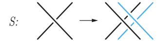
Figure 1. Doubling of $S$

Recall the definition of simplicial groups (see [44, p. 300] or [15]). A sequence of sets $X_{*}=\{X_{n}\}_{n\geq 0}$ is called a simplicial set if there are face maps:

$$d_{i}:X_{n}\longrightarrow X_{n-1}~{}\mbox{for}~{}0\leq i\leq n$$

and degeneracy maps

$$s_{i}:X_{n}\longrightarrow X_{n+1}~{}\mbox{for}~{}0\leq i\leq n,$$

that satisfy the following simplicial identities:

1. $d_{i}d_{j}=d_{j-1}d_{i}$ if $i<j$,

2. $s_{i}s_{j}=s_{j+1}s_{i}$ if $i\leq j$,

3. $d_{i}s_{j}=s_{j-1}d_{i}$ if $i<j$,

4. $d_{j}s_{j}=id=d_{j+1}s_{j}$,

5. $d_{i}s_{j}=s_{j}d_{i-1}$ if $i>j+1$.

Here $X_{n}$ can be geometrically viewed as the set of $n$-simplices including all possible degenerate simplices.

A simplicial group is a simplicial set $X_{*}$ such that each $X_{n}$ is a group and all face and degeneracy operations are group homomorphism.

Let us define a simplicial set $\mathrm{AB}_{*}=\{AB_{n}\}_{n\geq 0}$, where $AB_{n}=B_{n+1}$ and we assume that $B_{1}$ is the trivial group. There are face maps:

$$d_{i}:AB_{n}=B_{n+1}\longrightarrow AB_{n-1}=B_{n}~{}\mbox{for}~{}0\leq i\leq n,$$

that are deletion of the $(i+1)$-th strand and degeneracy maps

$$s_{i}:AB_{n}=B_{n+1}\longrightarrow AB_{n+1}=B_{n+2}~{}\mbox{for}~{}0\leq i\leq n,$$

that are doubling of the $(i+1)$-th strand. Hence, we have a simplicial set

$$\mathrm{AB}_{*}:\ \ \ \ldots\ \begin{matrix}\longrightarrow\\[-9.95845pt] \ldots\\[-7.11317pt] \longrightarrow\\[-9.95845pt] \longleftarrow\\[-9.95845pt] \ldots\\[-7.11317pt] \longleftarrow\end{matrix}\ B_{4}\ \begin{matrix}\longrightarrow\\[-9.95845pt] \longrightarrow\\[-9.95845pt] \longrightarrow\\[-9.95845pt] \longrightarrow\\[-9.95845pt] \longleftarrow\\[-9.95845pt] \longleftarrow\\[-9.95845pt] \longleftarrow\end{matrix}\ B_{3}\ \begin{matrix}\longrightarrow\\[-9.95845pt] \longrightarrow\\[-9.95845pt] \longrightarrow\\[-9.95845pt] \longleftarrow\\[-9.95845pt] \longleftarrow\end{matrix}\ B_{2}\ \begin{matrix}\longrightarrow\\[-9.95845pt] \longrightarrow\\[-9.95845pt] \longleftarrow\end{matrix}\ B_{1}.$$

It is easy to see that this simplicial set is not a simplicial group since the maps $d_{i}$ and $s_{i}$ are not group homomorphism.

Example 6.8.

If we take the action of $s_{0}$ on

$$B_{3}=\langle\sigma_{1},\sigma_{2}~{}||~{}\sigma_{1}\sigma_{2}\sigma_{1}=\sigma_{2}\sigma_{1}\sigma_{2}\rangle,$$

then $s_{0}(\sigma_{1})=e$ and $s_{0}(\sigma_{2})=\sigma_{2}$. Hence, the relation under the action of $s_{0}$ takes the form $\sigma_{2}=\sigma_{2}^{2}$, but it means that $\sigma_{2}=e.$

If we take the action of $d_{0}$ on $B_{3}$, we get

$$d_{0}(\sigma_{1})=\sigma_{2}\sigma_{1},~{}~{}d_{0}(\sigma_{2})=\sigma_{3},$$

and relation takes the form

$$\sigma_{2}\sigma_{1}\cdot\sigma_{3}\cdot\sigma_{2}\sigma_{1}=\sigma_{3}\cdot\sigma_{2}\sigma_{1}\cdot\sigma_{3}.$$

But considering the homomorphism $B_{4}$ to $S_{4}$ we see that this relation is not true in $B_{4}$.

Remark 6.9.

If one takes the pure braid groups instead of the braid groups then as was proved in [15, 24] the corresponding simplicial set is a simplcial group. But in the pure braid group $P_{3}$ we have relations

$$a_{12}a_{13}a_{23}=a_{23}a_{12}a_{13},~{}~{}a_{13}a_{23}a_{12}=a_{23}a_{12}a_{13},$$

which are not the same as the Yang–Baxter relation.

If we define the composition

$$D_{n}=s_{0}s_{1}\ldots s_{n-1}:B_{n}\to B_{2n},$$

that is the doubling of all strands, where we take the composition from the right to the left, then we get the next analogous of Corollary 6.15 in the braid group $B_{2n}$

Lemma 6.10.

The map

$$D_{n}=s_{0}s_{1}\ldots s_{n-1}:B_{n}\to B_{2n},$$

is a group homomorphism and

$$D_{n}(\sigma_{i})=\sigma_{2i}\sigma_{2i+1}\sigma_{2i-1}\sigma_{2i},~{}~{}i=1,2,\ldots,n-1.$$

Remark 6.11.

This statement can be illustrated by Figure 2, where the generators of $B_{n}$ are realized as braidings of pairs of strands.

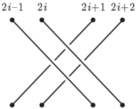
Figure 2. Pairs of strands

Example 6.12.

If we take the action of $D_{3}$ on $B_{3}$, we get the next subgroup of $B_{6}$

$$D_{3}(B_{3})=\langle\sigma_{2}\sigma_{1}\sigma_{3}\sigma_{2},~{}~{}\sigma_{4}\sigma_{3}\sigma_{5}\sigma_{4}~{}||~{}\sigma_{2}\sigma_{1}\sigma_{3}\sigma_{2}\cdot\sigma_{4}\sigma_{3}\sigma_{5}\sigma_{4}\cdot\sigma_{2}\sigma_{1}\sigma_{3}\sigma_{2}=\sigma_{4}\sigma_{3}\sigma_{5}\sigma_{4}\cdot\sigma_{2}\sigma_{1}\sigma_{3}\sigma_{2}\cdot\sigma_{4}\sigma_{3}\sigma_{5}\sigma_{4}\rangle.$$

Remark 6.13.

We defined the doubling $D_{n}$. By analogy we can define tripling and so on. More accurately put

$$D_{n}^{(k)}=s_{0}^{k}s_{1}^{k}\ldots s_{n-1}^{k}:B_{n}\to B_{(k+1)n},~{}~{}k=1,2,\ldots.$$

In particular $D_{n}^{(1)}=D_{n}$.

6.4. Doubling of the pure virtual braid group.

By using the same ideas as in the work [15, 24] on the classical braids in [12] it was introduced a simplicial group

$$\mathrm{VAP}_{*}:\ \ \ \ldots\ \begin{matrix}\longrightarrow\\[-9.95845pt] \ldots\\[-7.11317pt] \longrightarrow\\[-9.95845pt] \longleftarrow\\[-9.95845pt] \ldots\\[-7.11317pt] \longleftarrow\end{matrix}\ VP_{4}\ \begin{matrix}\longrightarrow\\[-9.95845pt] \longrightarrow\\[-9.95845pt] \longrightarrow\\[-9.95845pt] \longrightarrow\\[-9.95845pt] \longleftarrow\\[-9.95845pt] \longleftarrow\\[-9.95845pt] \longleftarrow\end{matrix}\ VP_{3}\ \begin{matrix}\longrightarrow\\[-9.95845pt] \longrightarrow\\[-9.95845pt] \longrightarrow\\[-9.95845pt] \longleftarrow\\[-9.95845pt] \longleftarrow\end{matrix}\ VP_{2}\ \begin{matrix}\longrightarrow\\[-9.95845pt] \longrightarrow\\[-9.95845pt] \longleftarrow\end{matrix}\ VP_{1}$$

on the pure virtual braid groups with $\mathrm{VAP}_{n}=VP_{n+1}$, the face homomorphism

$$d_{i}:\mathrm{VAP}_{n}=VP_{n+1}\longrightarrow\mathrm{VAP}_{n-1}=VP_{n}$$

given by deleting $(i+1)$-th strand for $0\leq i\leq n$, and the degeneracy homomorphism

$$s_{i}:\mathrm{VAP}_{n}=VP_{n+1}\longrightarrow\mathrm{VAP}_{n+1}=VP_{n+2}$$

given by doubling the $(i+1)$-th strand for $0\leq i\leq n$.

As in the case of braid group we can define the map

$$D_{n}^{(k)}=s_{0}^{k}s_{1}^{k}\ldots s_{n-1}^{k}:VP_{n}\to VP_{(k+1)n},~{}~{}k=1,2,\ldots.$$

In particular let us find the image of $VP_{3}$ under the action of $D_{3}=D_{3}^{(1)}$. We can do it using the formulas of actions of $s_{i}$ as on the generators of $VP_{3}$. These formulas were found in [11].

Proposition 6.14.

[11] The degeneracy map $s_{j}:VP_{n}\longrightarrow VP_{n+1}$, $j=0,1,\ldots,n-1$, acts on the generators $\lambda_{k,l}$ and $\lambda_{l,k}$, $1\leq k<l\leq n$, of $VP_{n}$ by the rules

$$s_{i-1}(\lambda_{k,l})=\left\{\begin{array}[]{lr}\lambda_{k+1,l+1}&for~{}i<k,\\ \lambda_{k,l+1}\lambda_{k+1,l+1}&for~{}i=k,\\ \lambda_{k,l+1}&for~{}k<i<l,\\ &\\ \lambda_{k,l+1}\,\lambda_{k,l}&for~{}i=l,\\ &\\ \lambda_{k,l}&for~{}i>l,\end{array}\right.$$

$$s_{i-1}(\lambda_{l,k})=\left\{\begin{array}[]{lr}\lambda_{l+1,k+1}&for~{}i<k,\\ \lambda_{l+1,k+1}\lambda_{l+1,k}&for~{}i=k,\\ \lambda_{l+1,k}&for~{}k<i<l,\\ &\\ \lambda_{l,k}\,\lambda_{l+1,k}&for~{}i=l,\\ &\\ \lambda_{l,k}&for~{}i>l.\end{array}\right.$$

Using this Proposition we can find

$$D_{3}(\lambda_{12})=s_{0}s_{1}s_{2}(\lambda_{12})=s_{0}s_{1}(\lambda_{12})=s_{0}(\lambda_{13}\lambda_{12})=\lambda_{14}\lambda_{24}\lambda_{13}\lambda_{23}=\lambda_{14}\lambda_{13}\lambda_{24}\lambda_{23},$$

and

$$D_{3}(\lambda_{13})=\lambda_{16}\lambda_{15}\lambda_{26}\lambda_{25},~{}~{}~{}D_{3}(\lambda_{23})=\lambda_{36}\lambda_{35}\lambda_{46}\lambda_{45}.$$

Since $D_{3}$ is a homomorphism $VP_{3}^{+}\to VP_{6}^{+}$ then the elements $D_{3}(\lambda_{12})$, $D_{3}(\lambda_{13})$ and $D_{3}(\lambda_{23})$ satisfy the Yang–Baxter relation

$$D_{3}(\lambda_{12})\,D_{3}(\lambda_{13})\,D_{3}(\lambda_{23})=D_{3}(\lambda_{12})\,D_{3}(\lambda_{13})\,D_{3}(\lambda_{23}).$$

On the other hand we have

$$D_{3}(\lambda_{12})=D_{3}(\rho_{1}\sigma_{1})=\rho_{2}\rho_{1}\rho_{3}\rho_{2}\cdot\sigma_{2}\sigma_{1}\sigma_{3}\sigma_{2}.$$

Hence, we constructed the group $Y_{3}$ and a homomorphism $\tau:Y_{3}\to VP_{6}$ Under the canonical homomorphism $VP_{6}\to VP_{6}^{+}$ which sends $\lambda_{ij}$ to $\lambda_{ij}$ and sends $\lambda_{ji}$ to $\lambda_{ij}^{-1}$ for $i<j$ the elements $N_{12},N_{13},N_{23}$ go to elements

$$M_{12}=\lambda_{14}\lambda_{13}\lambda_{24}\lambda_{23},~{}~{}M_{13}=\lambda_{16}\lambda_{15}\lambda_{26}\lambda_{25},~{}~{}M_{23}=\lambda_{36}\lambda_{35}\lambda_{46}\lambda_{45},$$

of $VP_{6}^{+}$, correspondingly. One can see that

$$D_{3}(\lambda_{12})=M_{12},~{}~{}D_{3}(\lambda_{13})=M_{13},~{}~{}D_{3}(\lambda_{23})=M_{23}.$$

Corollary 6.15.

In the group $\langle M_{12},M_{13},M_{23}\rangle\leq VP_{6}^{+}$ the following relation holds

$$M_{12}M_{13}M_{23}=M_{23}M_{13}M_{12}.$$

Remark 6.16.

Proposition 6.4 is less restrictive than Corollary 6.15, it does not demand the involutivity of the corresponding $R$-matrix.

Remark 6.17.

This Corollary is equivalent to the statement of Lemma 6.10. Indeed, one can see that

$$M_{12}=\lambda_{14}\lambda_{13}\lambda_{24}\lambda_{23}=\rho_{3}\rho_{2}\rho_{1}\sigma_{1}\rho_{2}\rho_{3}\cdot\rho_{2}\rho_{1}\sigma_{1}\rho_{2}\cdot\rho_{3}\rho_{2}\sigma_{2}\rho_{3}\cdot\rho_{2}\sigma_{2}=\rho_{2}\rho_{1}\rho_{3}\rho_{2}\cdot\sigma_{2}\sigma_{1}\sigma_{3}\sigma_{2}.$$

On the other side,

$$N_{12}=\lambda_{14}\lambda_{13}\lambda_{24}\lambda_{32}^{-1}=\rho_{3}\rho_{2}\rho_{1}\sigma_{1}\rho_{2}\rho_{3}\cdot\rho_{2}\rho_{1}\sigma_{1}\rho_{2}\cdot\rho_{3}\rho_{2}\sigma_{2}\rho_{3}\cdot\sigma_{2}^{-1}\rho_{2}=\rho_{2}\rho_{3}\rho_{1}\rho_{2}\cdot\sigma_{2}\sigma_{1}\sigma_{3}(\rho_{2}\sigma_{2}^{-1}\rho_{2}),$$

and we see that this element can be constructed from $\lambda_{12}$ using more complicated operation than doubling of strings.

Graphically the operation of constructing of set-theoretic solutions of the YBE on $B\times S$ is presented on Figure 3.

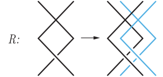
Figure 3. Doubling of $R$

Acknowledgement.

The parts 1, 2 and 4 of the work was caried out with the support of the Russian Science Foundation grant 20-71-10110. The work on parts 3, 5 and 6 was supported by the Ministry of Science and Higher Education of Russia (agreement No. 075-02-2021-1392).

References

• [1] N. Andruskiewitsch and M. Graña, From racks to pointed Hopf algebras, Adv. Math. 178 (2003), no. 2, 177–243.
• [2] V. G. Bardakov, The virtual and universal braids, Fund. Math., 181 (2004), 1–18.
• [3] V. G. Bardakov, P. BellingeriCombinatorial properties of virtual braids, Topology and its Applications, 156 (2009), 1071–1082.
• [4] V. G. Bardakov, R. Mikhailov, V. V. Vershinin and J. Wu, On the pure virtual braid group $PV_{3}$, Commun. in Algebra, 44, no. 3 (2016), 1350–1378.
• [5] V. G. Bardakov, P. Dey and M. Singh, Automorphism groups of quandles arising from groups, Monatsh. Math. 184 (2017), 519–530.
• [6] V. G. Bardakov, T. R. Nasybullov and Mahender Singh, Automorphism groups of quandles and related groups, Monatsh. Math. 189 (2019), 1-21.
• [7] V. G. Bardakov, I. B. S. Passi, and Mahender Singh, Quandle rings, J. Algebra Appl. 18 (2019), no. 8, 1950157, 23 pp, https://doi.org/10.1142/S0219498819501573.
• [8] V. G. Bardakov, Mahender Singh and Manpreet Singh, Free quandles and knot quandles are residually finite, Proc. Amer. Math. Soc. 147 (2019), no. 8, 3621–3633.
• [9] V. G. Bardakov, V. Gubarev, Rota–Baxter operators on groups, arXiv:2103.01848, 26 pp.
• [10] V. G. Bardakov, V. Gubarev, Rota–Baxter groups, skew left braces, and the Yang-Baxter equation, J. Algebra, 596 (2022), 1–24.
• [11] V. G. Bardakov, Jie Wu, Lifting theorem for the virtual pure braid groups, arXiv:2002.08686.
• [12] V. G. Bardakov, J. Wu, On virtual cabling and structure of $4$-strand virtual pure braid group, J. Knot Theory and Ram., 2020.
• [13] L. Bartholdi, B. Enriquez, P. Etingof and E. Rains, Groups and Lie algebras corresponding to the Yang-Baxter equations, J. Algebra, 305, no. 2 (2006), 742–764.
• [14] R. J. Baxter, Partition function of the eight-vertex lattice model. Ann. Physics, 70 (1972), 193–228.
• [15] A. J. Berrick, F. R. Cohen, Y. L. Wong, and J. Wu, Configurations, braids and homotopy groups, J. Amer. Math. Soc, 19, no. 2 (2006), 265–326.
• [16] M. Bonatto, Principal and doubly homogeneous quandles, Monatsh. Math. 191 (2020) 691–717.
• [17] K. S. Brown, Cohomology of groups. New York—Heidelberg-—Berlin, Springer, 1982, 308 pp. (Пер. на рус. яз.: Браун К. С, Когомологии групп. М.: Наука, 1987, 383 с.)
• [18] V. M. Bukhshtaber, Yang–Baxter mappings. (Russian) Uspekhi Mat. Nauk, 53, no. 6 (1998), 241–242; translation in Russian Math. Surveys 53, no. 6 (1998), 1343–1345.
• [19] V. M. Buchstaber, E. G. Rees, Multivalued groups and Hopf n-algebras, Uspekhi Mat. Nauk, 51:4(310) (1996), 149-150; Russian Math. Surveys, 51:4 (1996), 727-729.
• [20] J. Scott Carter, A survey of quandle ideas, Introductory lectures on knot theory, 22–53, Ser. Knots Everything, 46, World Sci. Publ., Hackensack, NJ (2012).
• [21] J. Scott Carter, D. Jelsovsky, S.Kamada, Laurel Langford and Masahico Saito, Quandle cohomology and state-sum invariants of knotted curves and surfaces, Trans. Amer. Math. Soc. 355 (2003), no. 10, 3947–3989.
• [22] F. Catino, I. Colazzo, and P. Stefanelli, The matched product of the solutions to the Yang-Baxter equation of finite order, arXiv:1904.07557v1, 19 pp.
• [23] V. Chari and A. Pressley, A guide to quantum groups, Cambridge University Press, Cambridge, 1995.
• [24] F. R. Cohen, J. Wu, Artin’s braid groups, free groups, and the loop space of the 2-sphere, Q. J. Math., 62, no. 4 (2011), 891–921.
• [25] V. Drinfeld. Quasi-Hopf algebras. Algebra i Analiz, 1(6):114–148, 1989.
• [26] V. G. Drinfeld, On some unsolved problems in quantum group theory, Quantum groups (Leningrad, 1990), 1–8, Lecture Notes in Math., 1510, Springer, Berlin, 1992.
• [27] M. Eisermann, Yang-Baxter deformations of quandles and racks, Algebr. Geom. Topol., 5 (2005), 537–562.
• [28] M. Elhamdadi, J. Macquarrie and R. Restrepo, Automorphism groups of Alexander quandles, J. Algebra Appl. 11 (2012), 1250008, 9 pp.
• [29] M. Elhamdadi, N. Fernando and B. Tsvelikhovskiy, Ring theoretic aspects of quandles, J. Algebra 526 (2019), 166–187.
• [30] R. Fenn and C. Rourke, Racks and links in codimension two, J. Knot Theory Ramifications, 1, no. 4 (1992), 343–406.
• [31] A. Ghobadi, Drinfeld Twists on Skew Braces, arXiv:2105.03286v1.
• [32] L. Guo, An Introduction to Rota–Baxter Algebra. Surveys of Modern Mathematics, vol. 4, International Press, Somerville (MA, USA); Higher education press, Beijing, 2012.
• [33] L. Guo, H. Lang, and Yu. Sheng, Integration and geometrization of Rota–Baxter Lie algebras, Adv. Math., 387 (2021), 107834.
• [34] D. Joyce, An algebraic approach to symmetry with applications to knot theory, PhD Thesis, University of Pennsylvania, 1979. vi+63 pp.
• [35] D. Joyce, A classifying invariant of knots, the knot quandle, J. Pure Appl. Algebra, 23 (1982), 37–65.
• [36] S. Kamada, Knot invariants derived from quandles and racks, Invariants of knots and 3-manifolds (Kyoto, 2001), 103–117 (electronic), Geom. Topol. Monogr., 4, Geom. Topol. Publ., Coventry, (2002).
• [37] C. Kassel, Quantum groups,
• [38] L. H. Kauffman, Virtual knot theory, Eur. J. Comb., 20, no. 7 (1999), 663–690.
• [39] P. Kulish, A. Mudrov On twisting solutions to the Yang-Baxter equation, 2000 Czechoslovak Journal of Physics 50(1): 115-122 DOI: 10.1023/A:1022885317520
• [40] V. Lebed, L. Vendramin On structure groups of set-theoretic solutions to the Yang-Baxter equation, Proc. Edinb. Math. Soc. (2) 62 (2019), no. 3, 683-717.
• [41] O. Loos, Reflexion spaces and homogeneous symmetric spaces, Bull. Amer. Math. Soc. 73 (1967) 250–253.
• [42] M. Markl, Operads and PROPs. Handbook of Algebra, 2008, 87–140. doi:10.1016/s1570-7954(07)05002-4.
• [43] S. Matveev, Distributive groupoids in knot theor, Mat. Sb. (N.S.), 119 (161), no. 1 (9), 1982, 78–88 (in Russian).
• [44] R. Mikhailov and I. B. S. Passi, Lower Central and Dimension Series of Groups, Lecture Notes in Mathematics, 1952, Springer-Verlag Berlin Heidelberg, 2009.
• [45] T. Nosaka, On quandle homology groups of Alexander quandles of prime order, Trans. Amer. Math. Soc. 365 (2013), 3413–3436.
• [46] M. M. Preobrazhenskaya, D. V. Talalaev, Group extensions, fiber bundles, and a parametric Yang–Baxter equation, Theoret. and Math. Phys., 207:2 (2021), 670–677.
• [47] L. Rabenda, mémoire de DEA, Université de Bourgogne (2003).
• [48] Reshetikhin, N. Y., Semenov-Tian-Shansky, M. A. (1988). Quantum R-matrices and factorization problems. Journal of Geometry and Physics, 5(4), 533–550. doi:10.1016/0393-0440(88)90018-6
• [49] М. А. Семенов Тянь-Шанский, Пуассоновы группы и одевающие преобразования, Записки научн. сем. ЛОМИ, 150 (1986), 119–142.
• [50] M. A. Semenov-Tian-Shansky, What is a classical r-matrix?, Funct. Anal. Appl., 17, no. 4 (1983), 259–272.
• [51] A. Soloviev, Non-unitary set-theoretical solutions to the quantum Yang-Baxter equation, Math. Res. Lett., 7, no. 5-6 (2000), 577–596.
• [52] M. Szymik, Quandle cohomology is a Quillen cohomology. Trans. Amer. Math. Soc. 371, no. 8 (2019), 5823–5839.
• [53] E. K. Sklyanin, L. A. Takhtadzhyan, and L. D. Faddeev, The quantum inverse problem method. I, Teor. Mat. Fiz. 40 (1979), no. 2, 194–220; English transl., Theor. and Math. Phys. 40, no. 2 (1979).
• [54] L. A. Takhtadzhyan and L. D. Faddeev, The quantum method for the inverse problem and the XYZ Heisenberg model, Uspekhi Mat. Nauk 34 (1979), no. 5, 13–63; English transl. in Russian Math. Surveys 34, no. 5 (1979).
• [55] A. B. Zamolodchikov, Tetrahedra equations and integrable systems in three dimensional space, Zh. Eksp. Teor. Fiz. 79 (1980) 641664. [English translation: Soviet Phys. JETP 52 (1980) 325–326].
• [56] A. B. Zamolodchikov, Tetrahedron equations and the relativistic S-matrix of straight-strings in 2+1 dimensions, Commun. Math. Phys., 79 (1981), 489–505.
• [57] C. N. Yang, Some exact results for the many-body problem in one dimension with repulsive delta-function interaction. Phys. Rev. Lett., 19 (1967), 1312–1315.
• [58] A. P. Veselov, Integrable maps, Russian Math. Surveys, 46:5 (1991), 1–51
• [59] A. P. Veselov, Yang-Baxter maps and integrable dynamics, Phys.Lett.A 314 (2003) 214
• [60] Vladimir V. Bazhanov, Sergey M. Sergeev, Yang–Baxter maps, discrete integrable equations and quantum groups, Nucl.Phys.B 926 (2018) 509-543.
• [61] V. Lebed, A. Vendramin, Homology of left non-degenerate set-theoretic solutions to the Yang-Baxter equation, Advances Math. 304 (2017), 1219-1261