A reduced order model for domain decompositions with non-conforming interfaces

Abstract

In this paper we propose a reduced order modeling strategy for two-way Dirichlet-Neumann parametric coupled problems solved with domain-decomposition (DD) sub-structuring methods. We split the original coupled differential problem into two sub-problems with Dirichlet and Neumann interface conditions, respectively. After discretization by (e.g.) the finite element method, the full-order model (FOM) is solved by Dirichlet-Neumann iterations between the two sub-problems until interface convergence is reached. We, then, apply the reduced basis (RB) method to obtain a low-dimensional representation of the solution of each sub-problem. Furthermore, we use the discrete empirical interpolation method (DEIM) applied at the interface level to achieve a fully reduced-order representation of the DD techniques implemented. To deal with interface data when non-conforming FE interface discretizations are considered, we employ the INTERNODES method combined with the interface DEIM reduction. The reduced-order model (ROM) is then solved by sub-iterating between the two reduced-order sub-problems until convergence of the approximated high-fidelity interface solutions. The ROM scheme is numerically verified on both steady and unsteady coupled problems, in the case of non-conforming FE interfaces.

1 Introduction

Reduced order modeling (ROM) techniques are numerical methods able to solve differential problems several orders of magnitude faster than conventional, high-fidelity full order models (FOMs), achieving real-time decision making and operational modeling in several contexts, ranging from fluid dynamics [1, 2, 3, 4, 5, 6] to biomedicine [7, 8, 9].

In several cases, domain decomposition (DD) [10, 11] techniques are necessary to (i) split the domain in two or more regions in which either the same or different methods are used to approximate the solution [12, 13, 14, 15], to (ii) solve systems that stem from the assembly of independently generated meshes [16, 17, 18] or to (iii) frame coupled problems where the physical nature of the involved submodels is very different [19]. In the last two cases, interface non-conformity issues can arise and ad-hoc techniques, such as, e.g. the MORTAR method [20, 21, 22] or the INTERNODES method [23, 24, 25] are to be implemented in order to ensure the correct exchange of information at the interface.

Domain decomposition schemes coupled with ROM techniques, especially the reduced basis (RB) method [26, 27, 28], have been first used in [29], where ROMs are applied only on small regions of the domains, for instance for PDEs with discontinuous solutions in those regions where the discontinuity occurs. Similar strategies have been implemented to tackle the numerical simulation of problems in fluid dynamics [30, 31, 32, 33, 34, 35, 36], aerospace engineering [37] and structural mechanics [38, 39], as well as for the optimization of complex systems [40, 41]. A common feature shared by several of these works is the application of a reduced order model in small parts of the domains. Interface conditions, on the other hand, have been usually treated in high-fidelity form through the application of different techniques, e.g. Lagrangian multipliers or Fourier basis functions, for sub-iterating schemes and/or solving the coupled model in monolithic form, naturally imposing interface constraints. In [42] also Dirichlet and Neumann data on conforming interfaces data are also considered in reduced form, while the Dirichlet-Neumann DD iterations structure is preserve by the reduced algorithm. However, at our knowledge, interface non-conformity has never been considered, given its intrinsic complexity.

In this work, we present a Dirichlet-Neumann DD-ROM relying on the RB method able to transfer interface data across non-conforming interfaces. In particular, we consider parametric second-order elliptic and/or parabolic problems solved with Dirichlet-Neumann sub-structuring domain decomposition algorithms. Therefore, we split the problem domain into two non-overlapping subdomains with a common interface and we define two parametrized subproblems with Dirichlet or Neumann interface conditions. RB methods are then applied at the subproblems level to approximate both the subproblems solution together with the Dirichlet or Neumann interface conditions.

To solve the coupled problem and compute the snapshots (for different parameter instances) required to train our ROM, we rely on the finite element (FE) method as high-fidelity FOM. In particular, the FOM solution is sought by sub-iterating between the two submodels solutions until convergence, being this latter reached when the difference between the solution at both sides of the interface falls under a prescribed tolerance. In presence of a non-conforming interface, FOM solutions can be sought through FE based methods such as the MORTAR method or the INTERNODES. In our code, however, we surrogate the non-conforming coupling by solving for each selected parameter instance the coupled problems twice: indeed, we define two possible FE discretizations in the complete domain (each one being obtained by extending to the other subdomain the spatial discretization set in the first one) and compute the solution of each subproblem using both discretizations, one for each simulation, featuring interface conformity. Then, we extract the solution of each of the subproblems (in the discretization originally set for the corresponding subdomain), therefore obtaining two sets of solution snapshots as well as the corresponding Dirichlet and Neumann traces at the common interface that can be seen as the original model solution when interface nonconformity is considered (see Remark 3 and Fig. 1).

The RB method is then applied to define a low-dimensional representation of the solution in each subdomain, while the discrete empirical interpolation method (DEIM) is applied to both Dirichlet and Neumann interface data in order to achieve a fully reduced-order representation of the DD method adopted. In the online phase, a Galerkin projection is used to reduce the subproblems’ dimension obtaining two reduced order subproblems. The solution of the coupled problem, for any new parameter instance, is then found by iterating between the solutions of the two reduced subproblems until (a suitable norm of) the difference between the two solutions at the interface, once traced back at the high-fidelity level, falls below a prescribed tolerance. In this phase, we transfer Dirichlet and Neumann interface data by applying the INTERNODES method and by using the DEIM as well as a low-order piecewise constant interpolation. This approach, which extends the work presented in [43] is still modular, and allows us to achieve a complete reduction of the model at hand, which can be seen as a two-way coupled model, including interface non-conforming grids cases.

The organization of the paper is the following: in Section 2 we present the formulation and the high-fidelity discretization of the parametrized problem, considering both steady and unsteady cases. Section 3 is devoted to the reduced-order formulation of the two sub-problems, while Section 4 is dedicated to the interface Dirichlet and Neumann reduced formulation. In Section 5, the algorithm is numerically verified by means of two test cases dealing with second-order linear PDEs, considering both an elliptic and a parabolic problem. Section 6 then reports some final remarks and possible perspectives of this work.

2 Two-way coupled problem and its FE discretization

We introduce the parameter dependent two-way coupled problem. Such problem can arise from the application of splitting domain decomposition methods to single-physics or multi-physics models. Let us start from the single-physics case, defined on a open bounded domain $\Omega\subset\mathbb{R}^{n}$, $(n=2,3)$ with Lipschitz boundary $\partial\Omega$. $\partial\Omega_{D}$ and $\partial\Omega_{N}$ denote the Dirichlet and the Neumann boundary, such that $\overline{\partial\Omega_{D}}\cup\overline{\partial\Omega_{N}}=\partial\Omega$ and $\partial\Omega_{D}\cap\partial\Omega_{N}=0$. Given the set of parameters $\boldsymbol{\mu}\in\mathscr{P}^{d}$, $d\geq 1$, we search for $u(\boldsymbol{\mu})$ in $\Omega$ such that

$$\begin{cases}\mathcal{L}(\boldsymbol{\mu})u(\boldsymbol{\mu})=f(\boldsymbol{\mu})&\text{in }\Omega\\ u(\boldsymbol{\mu})=g_{D}(\boldsymbol{\mu})&\text{on }\partial\Omega_{D}\\ \partial_{\mathcal{L}(\boldsymbol{\mu})}u(\boldsymbol{\mu})=g_{N}(\boldsymbol{\mu})&\text{on }\partial\Omega_{N},\end{cases}$$ (1)

where $\mathcal{L}(\boldsymbol{\mu})$ is a second-order elliptic operator, $f(\boldsymbol{\mu})$, $g_{D}(\boldsymbol{\mu})$ and $g_{N}(\boldsymbol{\mu})$ are functions defined in $\Omega$, $\partial\Omega_{D}$ and $\partial\Omega_{N}$, respectively, and $\partial_{\mathcal{L}(\boldsymbol{\mu})}u(\boldsymbol{\mu})$ is the conormal derivative associated with the operator $\mathcal{L}(\boldsymbol{\mu})$ on $\partial\Omega$.

Now, we split the computational domain $\Omega$ into two non-overlapping subdomains $\Omega_{1}$ and $\Omega_{2}$ with Lipschitz boundary $\partial\Omega_{i}$, $i=1,2$ and a common interface $\Gamma:=\partial\Omega_{1}\cap\partial\Omega_{2}$. For each $i=1,2$, we call $\partial\Omega_{i,D}=\partial\Omega_{i}\cap\partial\Omega_{D}$ and $\partial\Omega_{i,N}=\partial\Omega_{i}\cap\partial\Omega_{N}$.

The two-domains formulation of model (1) reads [11]:

$$\begin{cases}\mathcal{L}_{i}(\boldsymbol{\mu})u_{i}(\boldsymbol{\mu})=f(\boldsymbol{\mu})&\text{in }\Omega_{i},~{}i=1,2\\ u_{1}(\boldsymbol{\mu})=u_{2}(\boldsymbol{\mu})&\text{on }\Gamma\\ \partial_{\mathcal{L}_{1}(\boldsymbol{\mu})}u_{1}(\boldsymbol{\mu})+\partial_{\mathcal{L}_{2}(\boldsymbol{\mu})}u_{2}(\boldsymbol{\mu})=0&\text{on }\Gamma.\end{cases}$$ (2)

The Dirichlet-Neumann iterative scheme [11, 44] is applied to solve (2). Therefore, starting from the initial guesses $u_{1}^{0}(\boldsymbol{\mu})$ and $u_{2}^{0}(\boldsymbol{\mu})$, for each $k\geq 0$, we search for $u_{1}^{k+1}(\boldsymbol{\mu})$ in $\Omega_{1}$ and $u_{2}^{k+1}(\boldsymbol{\mu})$ in $\Omega_{2}$ such that

$$[left={\empheqlbrace} \mathcal{L}_{1}(\boldsymbol{\mu})u_{1}^{k+1}(\boldsymbol{\mu})=f(\boldsymbol{\mu}) \text{in }\Omega_{1}$$ (3a)

$$u_{1}^{k+1}(\boldsymbol{\mu})=u_{2}^{k}(\boldsymbol{\mu}) \text{on }\Gamma$$ (3b)

$$u_{1}^{k+1}(\boldsymbol{\mu})=g_{D}(\boldsymbol{\mu}) \text{on }\partial\Omega_{1,D}$$ (3c)

$$\partial_{\mathcal{L}_{1}(\boldsymbol{\mu})}u_{1}^{k+1}(\boldsymbol{\mu})=g_{N}(\boldsymbol{\mu}) \text{on }\partial\Omega_{1,N}$$ (3d)

and

$$[left={\empheqlbrace}] \mathcal{L}_{2}(\boldsymbol{\mu})u_{2}^{k+1}(\boldsymbol{\mu})=f(\boldsymbol{\mu}) \text{in }\Omega_{2}$$ (3da)

$$\partial_{\mathcal{L}_{2}(\boldsymbol{\mu})}u_{2}^{k+1}(\boldsymbol{\mu})-\partial_{\mathcal{L}_{1}(\boldsymbol{\mu})}u_{1}^{k+1}(\boldsymbol{\mu})=0 \text{on }\Gamma$$ (3db)

$$u_{2}^{k+1}(\boldsymbol{\mu})=g_{D}(\boldsymbol{\mu}) \text{on }\partial\Omega_{2,D}$$ (3dc)

$$\partial_{\mathcal{L}_{2}(\boldsymbol{\mu})}u_{2}^{k+1}(\boldsymbol{\mu})=g_{N}(\boldsymbol{\mu}) \text{on }\partial\Omega_{2,N},$$ (3dd)

where $\partial_{\mathcal{L}_{i}(\boldsymbol{\mu})}\mathbf{u}(\boldsymbol{\mu})$ is the conormal derivative associated with the operator $\mathcal{L}_{i}(\boldsymbol{\mu})$ on $\partial\Omega_{i}$. Moreover, a relaxation techniques [11] is usually applied to ensure and accelerate the scheme convergence.

Then, we name the problem and the corresponding solution set in $\Omega_{1}$ slave model and slave solution, and the ones set in $\Omega_{2}$ master model and master solution, respectively.

For each $i=1,2$, we first define the local spaces

$$V_{i}=\{v\in H^{1}(\Omega_{i}) ~{}|~{}v=0\text{ on }\partial\Omega_{i,D}\}\quad\text{and}\quad V_{i}^{0}=\{v\in V_{i}~{}|~{}v=0\text{ on }\Gamma\},$$ (3e)

and the space of traces of the elements of $V$ on the interface $\Gamma$, meaning

$$\Lambda=\{\lambda\in H^{1/2}(\Gamma) ~{}|~{}\exists v\in V:v_{|\Gamma}=\lambda\}.\vspace{-0.05cm}$$ (3f)

Moreover, we denote by $\mathcal{R}_{i}:\Lambda\rightarrow V_{i}\ \text{ s.t. }(\mathcal{R}_{i}\eta)_{|\Gamma}=\eta\text{ }\forall\eta\in\Lambda$ any possibile linear and continuous lifting operator from the interface $\Gamma$ to $\Omega_{i}$.

We consider two a-priori independent discretizations $\mathcal{T}_{h_{1}}$ and $\mathcal{T}_{h_{2}}$ on the domains $\Omega_{1}$ and $\Omega_{2}$ that can imply a mesh non-conformity at the interface. For instance, $\mathcal{T}_{h_{i}}$ can be made of simplices (triangles of tetrahedra) or quads (quadrilaterals or hexahedra), depending on the mesh size, a positive parameter $h_{i}>0$. Moreover, different mesh sizes $h_{1}$ and $h_{2}$, or different polynomial degrees $p_{1}$ or $p_{2}$, can be selected. Then, we call $\Gamma_{1}$ and $\Gamma_{2}$ the internal interfaces induced by $\mathcal{T}_{h_{1}}$ and $\mathcal{T}_{h_{2}}$ of $\Omega_{1}$ and $\Omega_{2}$, respectively: we talk of geometrical conformity if $\Gamma_{1}=\Gamma_{2}$ and of geometrical non-conformity if $\Gamma_{1}\not=\Gamma_{2}$. Finally, we assume that for any $T_{i,m}\in\mathcal{T}_{h_{i}}$, $\partial T_{i,m}\cap\partial\Omega$ fully belongs to $\partial\Omega_{i,D}$ or $\partial\Omega_{i,N}$, and that the interfaces $\Gamma_{i}$ do not cut any $T_{i,m}\in\mathcal{T}_{h_{i}}$. According to the test cases in Section 5, hereon we consider only quads elements.

For each partition $\mathcal{T}_{h_{i}}$ we define the finite element approximation spaces as

$$X_{h_{i}}^{q_{i}}=\{v\in C^{0}(\overline{\Omega_{i}}):v_{|T_{i,m}}\circ F_{i,m}\in\mathbb{Q}_{q_{i}},\forall T_{i,m}\in\mathcal{T}_{h_{i}}\},$$

in which $F_{i,m}$ is a smooth bijection that maps the reference quad $(-1,1)^{n}$ into the quad $T_{i,m}$, and $q_{i}$ are chosen integers. The finite dimensional spaces to define the discrete formulation of the exploited problems will be

$$V_{h_{i}}=\{v\in X_{h_{i}}^{q_{i}}:v_{|\partial\Omega_{i,D}}=0\},\quad V_{h_{i}}^{0}=\{v\in V_{h_{i}},v_{|\Gamma}=0\},\quad i=1,2,$$ (3g)

while the spaces of traces on $\Gamma$ are

$$Y_{h_{i}}=\{\lambda=v_{|\Gamma},v\in X_{h_{i}}\}\quad\text{ and }\quad\Lambda_{h_{i}}=\{\lambda=v_{|\Gamma},v\in V_{h_{i}}\}.$$ (3h)

Then, for $i=1,2$, we set the linear and continuous discrete lifting operator

$$\mathcal{R}_{h_{i}}:\Lambda_{h_{i}}\rightarrow V_{h_{i}},\quad\text{ s.t. }\quad(\mathcal{R}_{h_{i}}\eta_{h_{i}})_{|\Gamma}=\eta_{h_{i}},\quad\forall\eta_{h_{i}}\in\Lambda_{h_{i}}.$$ (3i)

In a practical implementation, $\mathcal{R}_{h_{i}}\eta_{h_{i}}$ is a finite element interpolant that imposes the same values of $\eta_{h_{i}}$ at the FE nodes of $\Gamma$ and zeros at any other FE node of $\mathcal{T}_{h_{i}}\backslash\Gamma_{i}$.

We also introduce two independent transfer operators able to exchange information between the independent grids on the interface $\Gamma$, namely

$$\Pi_{12}:Y_{h_{2}}\rightarrow Y_{h_{1}}\quad\text{and}\quad\Pi_{21}:Y_{h_{1}}\rightarrow Y_{h_{2}}.$$

In the non-conforming case, if $\Gamma_{1}$ and $\Gamma_{2}$ coincide, such operators could be the classical Lagrange interpolation operators, while $\Pi_{jk}$ are the identity operators when the meshes are conforming. Instead, if the mesh are non-conforming and $\Gamma_{1}\not=\Gamma_{2}$, $\Pi_{12}$ and $\Pi_{21}$ could be, e.g., Rescaled Localized Radial Basis Function operators, as for the INTERNODES [23, 25, 45].

To exploit a FE-Galerkin approximation to set the high-fidelity FOM and get the algebraic formulation of problems (3) and (3d), it is useful to consider local vectors and matrices. In particular, we define the following set of indices associated with the nodes $\mathbf{x}_{i}\in\mathcal{T}_{h_{i}}$:

$$\begin{split}&\mathcal{I}_{\overline{\Omega}_{i}}=\{1,\dots,N_{i}\},\qquad\mathcal{I}_{i}=\{j\in\mathcal{I}_{\overline{\Omega}_{i}}:\mathbf{x}_{j}\in\overline{\Omega}_{i}\backslash(\overline{\partial\Omega_{D,i}}\cup\mathring{\Gamma_{i}})\}\\ &\mathcal{I}_{\Gamma_{i}}=\{j\in\mathcal{I}_{\overline{\Omega}_{i}}:\mathbf{x}_{j}\in\overline{\Gamma_{i}}\},\qquad\mathcal{I}_{D_{i}}=\{j\in\mathcal{I}_{\overline{\Omega}_{i}}:\mathbf{x}_{j}\in\overline{\partial\Omega_{D,i}}\},\end{split}$$ (3j)

being $N_{i}$ the cardinality of $\mathcal{I}_{\overline{\Omega}_{i}}$.

Then, for each $i=1,2$, we set the local stiffness matrices $\mathbb{A}_{i}(\boldsymbol{\mu})$ so that

$$\mathbb{A}_{i,i}(\boldsymbol{\mu})=\mathbb{A}_{i}(\mathcal{I}_{i},\mathcal{I}_{i};\boldsymbol{\mu})$$

is the submatrix of $\mathbb{A}_{i}(\boldsymbol{\mu})$ of the rows and columns of $\mathbb{A}_{i}(\boldsymbol{\mu})$ whose indices belong to $\mathcal{I}_{i}$, i.e. either the internal nodes of $\Omega_{i}$ and those on $\partial\Omega_{i,N}$. Similarly, we can define $\mathbb{A}_{\Gamma_{i},\Gamma_{i}}(\boldsymbol{\mu})=\mathbb{A}_{i}(\mathcal{I}_{\Gamma_{i}},\mathcal{I}_{\Gamma_{i}};\boldsymbol{\mu})$, $\mathbb{A}_{i,\Gamma_{i}}(\boldsymbol{\mu})=\mathbb{A}_{i}(\mathcal{I}_{i},\mathcal{I}_{\Gamma_{i}};\boldsymbol{\mu})$, $\mathbb{A}_{\Gamma_{i},i}(\boldsymbol{\mu})=\mathbb{A}_{i}(\mathcal{I}_{\Gamma_{i}},\mathcal{I}_{i};\boldsymbol{\mu})$ and $\mathbb{A}_{i,D}(\boldsymbol{\mu})=\mathbb{A}_{i}(\mathcal{I}_{i},\mathcal{I}_{D_{i}};\boldsymbol{\mu})$.

Moreover, if $\mathbf{f}_{N_{i}}(\boldsymbol{\mu})$ and $\mathbf{u}_{N_{i}}(\boldsymbol{\mu})$ are the right hand side vector and the vector of degrees of freedom of the approximated solution in $\overline{\Omega_{i}}$, respectively, we set

$$\mathbf{f}_{i}(\boldsymbol{\mu})=\mathbf{f}_{N_{i}}(\mathcal{I}_{i};\boldsymbol{\mu}),\quad\mathbf{f}_{\Gamma_{i}}(\boldsymbol{\mu})=\mathbf{f}_{N_{i}}(\mathcal{I}_{\Gamma};\boldsymbol{\mu}),$$

$$\mathbf{u}_{i}(\boldsymbol{\mu})=\mathbf{u}_{N_{i}}(\mathcal{I}_{i};\boldsymbol{\mu}),\quad\mathbf{u}_{\Gamma_{i}}(\boldsymbol{\mu})=\mathbf{u}_{N_{i}}(\mathcal{I}_{\Gamma};\boldsymbol{\mu}).$$

Then, by applying the INTERNODES method (see, e.g. [25]) the algebraic form of $\eqref{eq:master_FOM}$ reads as : for each $k\geq 0$, find $\mathbf{u}_{1}^{k+1}(\boldsymbol{\mu})$ solution of

$$\begin{cases}\mathbb{A}_{1,1}(\boldsymbol{\mu})\mathbf{u}_{1}^{k+1}(\boldsymbol{\mu})=\mathbf{f}_{1}(\boldsymbol{\mu})-\mathbb{A}_{1,D}(\boldsymbol{\mu})\mathbf{g}_{D,1}(\boldsymbol{\mu})-\mathbb{A}_{1,\Gamma_{1}}(\boldsymbol{\mu})\mathbf{u}_{\Gamma_{1}}^{k+1}(\boldsymbol{\mu})\\ \mathbf{u}_{\Gamma_{1}}^{k+1}(\boldsymbol{\mu})=\mathbb{R}_{12}\mathbf{u}_{\Gamma_{2}}^{k}(\boldsymbol{\mu}).\end{cases}$$ (3k)

where $\mathbb{R}_{12}$ is the rectangular matrix associated with $\Pi_{12}$.

The algebraic formulation of problem $\eqref{eq:slave_FOM}$ reads as: for each $k\geq 0$, find $\mathbf{u}_{2}^{k+1}(\boldsymbol{\mu})$ such that

$$\begin{cases}\mathbb{A}_{2,2}(\boldsymbol{\mu})\mathbf{u}_{2}^{k+1}(\boldsymbol{\mu})=\mathbf{f}_{2}(\boldsymbol{\mu})+\mathbf{r}_{N_{2}}^{k+1}(\boldsymbol{\mu})-\mathbb{A}_{2,D}(\boldsymbol{\mu})\mathbf{g}_{D,2}(\boldsymbol{\mu})\\ \mathbf{r}_{N_{2}}^{k+1}(\boldsymbol{\mu})=-\mathbb{M}_{\Gamma_{2}}\mathbb{R}_{21}\mathbb{M}_{\Gamma_{1}}^{-1}\mathbf{r}_{N_{1}}^{k+1}(\boldsymbol{\mu}),\end{cases}$$ (3l)

where, for $i=1,2$, $\mathbb{M}_{\Gamma_{i}}$ is the interface mass matrix on $\Gamma_{i}$ and $\mathbb{R}_{21}$ is the matrix associated with $\Pi_{21}$, while

$$\mathbf{r}_{N_{i}}^{k+1}(\boldsymbol{\mu})=\left(\mathbb{A}_{i}(\boldsymbol{\mu})\mathbf{u}_{N_{i}}^{k+1}(\boldsymbol{\mu})-\mathbf{f}_{i}(\boldsymbol{\mu})\right)_{|\Gamma_{i}}.$$ (3m)

Therefore, the complete solutions of subproblems (3) and (3d) are

$$\mathbf{u}_{N_{i}}^{k+1}(\boldsymbol{\mu})=\left[\begin{matrix}\mathbf{u}_{i}^{k+1}(\boldsymbol{\mu})\\ \mathbf{u}_{\Gamma_{i}}^{k+1}(\boldsymbol{\mu})\\ \mathbf{g}_{D,i}(\boldsymbol{\mu})\end{matrix}\right].$$

Further details on the derivation of these systems, which aree indeed quite standard in the DD literature, can be found, e.g., in [11, 25].

The residual vector is the algebraic counterpart of an element of the dual space $Y^{\prime}_{h_{i}}$ of $Y_{h_{i}}$ – see, e.g., [46, Chapter 3] – then we define by $\mathbf{z}_{N_{i}}(\boldsymbol{\mu})$ the element obtained from $\mathbf{r}_{N_{i}}(\boldsymbol{\mu})$ by solving

$$\mathbb{M}_{\Gamma_{i}}\mathbf{z}_{N_{i}}(\boldsymbol{\mu})=\mathbf{r}_{N_{i}}(\boldsymbol{\mu}).$$ (3n)

Here $\mathbf{z}_{N_{i}}(\boldsymbol{\mu})$ is the algebraic counterpart of the Riesz’ element associated with the residual $\mathbf{r}_{N_{i}}(\boldsymbol{\mu})$. In other words, the interface mass matrix becomes the transfer matrix from the Lagrange basis to the dual one and viceversa [25, 47] and the array $\mathbf{z}_{N_{i}}(\boldsymbol{\mu})$ represents the residual in primal form.

Therefore, the matrix $\mathbb{R}_{21}$ transfer the function of $Y_{h_{1}}$ whose nodal values are stored in $\mathbf{z}_{N_{i}}$ (corresponding to the interface residual vectors $\mathbf{r}_{N_{1}}$) at the nodes on $\Gamma_{2}$.

Note that the conforming interface case can be recovered by taking $\mathbb{R}_{12}$ and $\mathbb{M}_{\Gamma_{2}}\mathbb{R}_{21}\mathbb{M}_{\Gamma_{1}}^{-1}$ both equal to the identity matrix.

Remark 1.

When $\partial\Gamma_{i}\cap\partial\Omega_{i,D}\not=0$, the residual $\mathbf{r}_{N_{i}}$ should be corrected to take into account the interpolation process on all the degrees of freedom of $\Gamma_{i}$, including those on $\partial\Gamma_{i}$ (see e.g. [25]). Even if the reduced technique presented in this paper will work in both cases, hereon we will consider only $\partial\Gamma_{i}\cap\partial\Omega_{i,D}=0$.

Remark 2.

The above formulation can be easily extended to time-dependent second-order parabolic PDE problems. In such cases, suitable numerical schemes are implemented to handle the time discretization and Dirichlet-Neumann subdomains iterations must be applied for each time step of the approximated solution [11]. The application of our method to a time-dependent test case will be addressed in Section 5.

Remark 3.

The master and the slave solution snapshots can be directly collected from the FOM computations by solving (3k)-(3m) when (i) conforming discretizations are considered in the two subdomains or (ii) when interpolation/projection methods are implemented to handle non-conforming grids, e.g. MORTAR methods or INTERNODES. In the non-conforming case, however, if FOM interpolation or projection methods are lacking, the snapshots for each subproblem can be surrogated solving for each parameter instance the FOM problem twice, i.e. with two different conforming discretizations. In particular, we first define two possible FE grids in the complete domains by setting on each first subdomain a chosen spatial discretization and extending it (conformingly) to the corresponding second one. Now, both coupled problems feature interface conformity and can be solved with Dirichlet-Neumann iterations. Then, we collect the snapshots of each subproblem and the relative interface data in the discretization set in the non-conforming case for the corresponding subdomain, obtaining two sets of solution and their Dirichlet and Neumann data. Indeed, this snapshots can be seen as the model solution when interface non-conformity is considered (see Fig. 1 for a schematic scatch of the used procedure). In this paper, such techniques is used to collect the snapshots for the test cases reported in Section 5.

Figure 1: Schematic representation of the two discretizations of the domain $\Omega$ used to compute the FOM snapshots (left and center) and the discretization of the domain $\Omega$ used to compute the ROM snapshots (right).

3 Master and slave reduced order problems

The strategy we propose here aims at both reducing separately the two subproblems and using reduced techniques to treat also the Dirichlet and Neumann interface conditions arising from the Dirichlet-Neumann subdomains iterations applied at the reduced level. In particular, this ROM technique is an extension of the one proposed in [43] and combines different RB methods, one set for each subproblem, and the DEIM to treat both the interface conditions, by defining independent reduced order representations of the involved quantities.

We first approximate the FOM solution of the master and slave models by means of a small number of basis functions defined in the corresponding subdomain $\Omega_{i}$ and selected through a POD procedure. Moreover, using the DEIM, we identify a suitable set of basis functions for the master and slave interface snapshots and use them to transfer Dirichlet and Neumann data across conforming or non-conforming interface grids. Lastly, considering the same Dirichlet-Neumann iteration scheme of the high-fidelity FOM, we iterate between the reduced solutions of the two subproblems imposing the continuity of both the interface solutions and fluxes at each iterations (see Fig. 2).

Figure 2: Schematic representation of the reduced order Dirichlet-Neumann domain decomposition algorithm.

The reduced form of master and slave problems is described in this Section, while we derive the procedure to reduce parameter-dependent Dirichlet and Neumann interface conditions in Section 4.

We define the reduced version of problems $\eqref{eq:master_steady_algebraic}$ and $\eqref{eq:slave_steady_algebraic}$ relying on a POD-Galerkin approach [46]. Therefore, in the offline stage we collect the set of snapshots solving the sub-FOMs for a suitable set of parameter values. In particular, we choose as snapshots the FOM slave and master solutions at convergence of the sub-iterations, i.e. $\mathbf{S}_{1}=\{\mathbf{u}_{1}(\boldsymbol{\mu}_{\ell}),\boldsymbol{\mu}_{\ell}\in\mathscr{P}^{d}\}$ and $\mathbf{S}_{2}=\{\mathbf{u}_{2}(\boldsymbol{\mu}_{\ell}),\boldsymbol{\mu}_{\ell}\in\mathscr{P}^{d}\}$, respectively. Sampling of the parameter space is usually done considering a latin hypercube sampling (LHS) method [48, 49].

Remark 4.

From now on, the index $k$ is omitted when quantities at convergence of the Dirichlet-Neumann FOM iterations are considered.

The POD technique is applied to each set of snapshots $\mathbf{S}_{1}$ and $\mathbf{S}_{2}$ and a corresponding set of reduced basis functions is computed and stored for the approximation of the solution on each subdomain. We denote by $n_{i}$ the cardinality of the set of reduced basis functions. Defining $\mathbb{V}_{i}\in\mathbb{R}^{N_{i}\times n_{i}}$, $n_{i}\ll N_{i}$, the matrices whose columns yield the obtained basis functions, the ROM seeks for an approximation of the FOM solutions under the form

$$\mathbf{u}_{1}(\boldsymbol{\mu})\approx\mathbb{V}_{1}\mathbf{u}_{n_{1}}(\boldsymbol{\mu})$$

and

$$\mathbf{u}_{2}(\boldsymbol{\mu})\approx\mathbb{V}_{2}\mathbf{u}_{n_{2}}(\boldsymbol{\mu}).$$

Projecting problems $\eqref{eq:master_steady_algebraic}$ and $\eqref{eq:slave_steady_algebraic}$ onto the reduced spaces defined by $\mathbb{V}_{i}$, starting from an initial guess $\mathbf{u}_{n_{i}}^{0}(\boldsymbol{\mu})$ and $\mathbf{u}_{n_{2}}^{0}(\boldsymbol{\mu})$, in the online phase, for each $k\geq 0$, we search for the reduced solutions $\mathbf{u}_{n_{1}}^{k+1}(\boldsymbol{\mu})\in\mathbb{R}^{n_{1}}$ and $\mathbf{u}_{n_{2}}^{k+1}(\boldsymbol{\mu})\in\mathbb{R}^{n_{2}}$ such that

$$\begin{cases}\mathbb{A}_{n_{1}}(\boldsymbol{\mu})\mathbf{u}_{n_{1}}^{k+1}(\boldsymbol{\mu})=\mathbf{f}_{n_{1}}(\boldsymbol{\mu})-\mathbb{V}_{1}^{T}\mathbb{A}_{1,D}(\boldsymbol{\mu})\mathbf{g}_{D,1}(\boldsymbol{\mu})-\mathbb{V}_{1}^{T}\mathbb{A}_{1,\Gamma_{1}}(\boldsymbol{\mu})\mathbf{u}_{\Gamma_{1}}^{k+1}(\boldsymbol{\mu})\\ \mathbf{u}_{\Gamma_{1}}^{k+1}(\boldsymbol{\mu})=\mathbb{R}_{12}\mathbf{u}_{\Gamma_{2}}^{k}(\boldsymbol{\mu})\end{cases}$$ (3o)

and

$$\begin{cases}\mathbb{A}_{n_{2}}(\boldsymbol{\mu})\mathbf{u}_{n_{2}}^{k+1}(\boldsymbol{\mu})=\mathbf{f}_{n_{2}}(\boldsymbol{\mu})+\mathbb{V}_{2}^{T}\mathbf{r}_{N_{2}}^{k+1}(\boldsymbol{\mu})-\mathbb{V}_{2}^{T}\mathbb{A}_{2,D}\mathbf{g}_{D,2}\\ \mathbf{r}_{N_{2}}^{k+1}(\boldsymbol{\mu})=-\mathbb{M}_{\Gamma_{2}}\mathbb{R}_{21}\mathbb{M}_{\Gamma_{1}}^{-1}\mathbf{r}_{N_{1}}^{k+1}(\boldsymbol{\mu}),\end{cases}$$ (3p)

where

$$\mathbb{A}_{n_{i}}(\boldsymbol{\mu})=\mathbb{V}_{i}^{T}\mathbb{A}_{i,i}(\boldsymbol{\mu})\mathbb{V}_{i},\qquad\mathbf{f}_{n_{i}}(\boldsymbol{\mu})=\mathbb{V}_{i}^{T}\mathbf{f}_{i}(\boldsymbol{\mu}),\qquad i=1,2.$$

Notice that the second equations in problems (3o) and (3p) (the interface equations) are defined in the FOM space, whereas the first ones are in the ROM space. The reduced version of the interface equations will be derived in the following Section.

Remark 5.

For simplicity, in this paper we only consider the case of linear PDE problems. In the case of nonlinear problems, the presence of nonlinear terms in the master and slave formulations can be handled through suitable hyper-reduction techniques like, e.g, the DEIM [50, 51, 52]. The ROM approach would be still modular, requiring the reduction of each subproblem and the treatment of interface data as shown in the next section.

Remark 6.

Time-dependent problems can be reduced with RB methods considering the time variable as an additional parameter of the model. Indeed, in such case the FOM solutions at each time step of the simulation are collected in the set of snapshots, and the reduced basis allows to approximate the time-dependent solution of each subproblem involving vectors of (reduced) degrees of freedom $\mathbf{u}_{n_{1}}$, $\mathbf{u}_{n_{2}}$ that are also time-dependent (see Section 5).

4 Parametric interface data reduction

Dealing with interface conditions highlighted, especially when using non-conforming grids, requires special care. Since the subproblems (3o) and (3p) are parameter-dependent, the interface data naturally inherit the parameter dependency and the DEIM [50, 51, 52, 53, 54, 55, 56] can be applied to both reduce the dimension of such data and to transfer the information across the interface grids. Indeed, using DEIM means: (i) compute a set of basis functions for the quantity of interest employing POD, (ii) use a greedy algorithm to identify a small number of dofs as weights for the corresponding basis functions (in place of the weights used in simple POD). The nodes corresponding to such dofs define the so-called reduced mesh, effectively determining a relation between the FE grids and the reduced space. Therefore, when considering interface reduction, a small number of interface nodes can be selected through the DEIM to described the complete vector of parametrized interface data. In the conforming case, DEIM can be used directly on the quantity of interest, i.e. the interface solution in case of Dirichlet data, or the interface residual in case of Neumann data. For non-conforming interface grids, the residuals (in primal form) must be involved to treat the Neumann terms [17].

In Subsection 4.1 and 4.2 we define the reduction of the Dirichlet and Neumann interface conditions, respectively, when non-conforming interface grids are considered. These new ROM interface conditions are used to substitute the interface equations of problems (3o) and (3p).

4.1 Parameter-dependent Dirichlet data

The parametric interpolation method of the Dirichlet data used in this work is similar to the one introduced in [43]. Such technique relies on the DEIM and can be applied in case of both conforming and non-conforming interface grids.

First, in the offline phase we collect from the slave domain $\Omega_{1}$ the interface snapshots, i.e. we extract the interface (Dirichlet) degrees of freedom obtained for different instances of the parameter vectors from the FOM computation. Notice that, as for the solution reduction, we select only the interface dofs at convergence of the FOM Dirichlet-Neumann iterations, namely

$$\mathbf{S}_{D}=\{\mathbf{u}_{\Gamma_{1}}(\boldsymbol{\mu}_{\ell}),~{}\boldsymbol{\mu}_{\ell}\in\mathscr{P}^{d}\}.$$

Let us denote by $N_{1,\Lambda}$ the number of FOM dofs on $\Gamma_{1}$. A low-dimensional representation of the interface dofs can then be computed by determining a set of $M_{1}\ll N_{1,\Lambda}$ POD basis functions from $\mathbf{S}_{D}$ that we store in the matrix $\boldsymbol{\Phi}_{D}$, with the purpose of getting

$$\mathbf{u}_{\Gamma_{1}}(\boldsymbol{\mu})\approx\boldsymbol{\Phi}_{D}\mathbf{u}_{1,M_{1}}(\boldsymbol{\mu}),$$

where $\mathbf{u}_{1,M_{1}}(\boldsymbol{\mu})$ is a vector of $M_{1}$ coefficients. Furthermore, with a greedy algorithm [54], we select iteratively $M_{1}$ indices in $\{1,\dots,N_{1,\Lambda}\}$, by minimizing the interpolation error over the interface snapshots set $\mathbf{S}_{D}$, according to the maximum norm. the set of such indices is denoted by

$$\mathcal{I}_{1,D}\subset\{1,\dots,N_{1,\Lambda}\},\quad\text{with cardinality }|\mathcal{I}_{1,D}|=M_{1}.$$ (3q)

The points corresponding to th indices of $\mathcal{I}_{1,D}$, are usually referred to as magic points on $\Gamma_{1}$, and are used to impose the Dirichlet interface conditions on $\Gamma_{1}$ for the reduced online problem. Let us denote by $\mathbf{u}_{\Gamma_{1,|\mathcal{I}_{1,D}}}(\boldsymbol{\mu})$ the vector of the FOM dofs at the magic points.

In the online phase, at each Dirichlet-Neumann iteration $k$, we ask that the reduced interface vector $\mathbf{u}_{1,M}^{k+1}(\boldsymbol{\mu})$ satisfies the relation

$$\boldsymbol{\Phi}_{D_{|\mathcal{I}_{1,D}}}\mathbf{u}_{1,M}^{k+1}(\boldsymbol{\mu})=\mathbf{u}_{\Gamma_{1_{|\mathcal{I}_{1,D}}}}^{k+1}(\boldsymbol{\mu}),$$

where $\boldsymbol{\Phi}_{D_{|\mathcal{I}_{1,D}}}\in\mathbb{R}^{M_{1}\times M_{1}}$ is the sub-matrix of $\boldsymbol{\Phi}_{D}$ containing the $\mathcal{I}_{1,D}$ rows specified in (see e.g. [52] for the well-posedness of the above procedure.). The FOM interface dofs on $\Gamma_{1}$ can be then approximated as

$$\mathbf{u}_{\Gamma_{1}}^{k+1}(\boldsymbol{\mu})\approx\boldsymbol{\Phi}_{D}\boldsymbol{\Phi}^{-1}_{D_{|\mathcal{I}_{1,D}}}\mathbf{u}_{\Gamma_{1_{|\mathcal{I}_{1,D}}}}^{k+1}(\boldsymbol{\mu}).$$ (3r)

Now we replace $\mathbf{u}_{\Gamma_{1_{|\mathcal{I}_{1,D}}}}^{k+1}$ with the values of the master solution $\mathbf{u}_{N_{2}}^{k}$ at other points on $\Gamma_{2}$, the ones corresponding to the magic points on $\Gamma_{1}$. Thus, given the position $\mathbf{p}_{1}$ of the magic point corresponding to the index $i_{1,D}\in\mathcal{I}_{1,D}$ in Cartesian coordinates, we search for the corresponding node in the master interface, i.e. for the point $\mathbf{p}_{2}\in\Gamma_{2}$ such that

$$\mathbf{p}_{2}=\min_{\mathbf{p}_{2}^{j}\in\text{nodes}_{\Gamma_{2}}}(\text{dist}(\mathbf{p}_{1}-\mathbf{p}_{2}^{j})).$$

Remark 7.

When the solution of the above minimization problem is not unique, we choose as $\mathbf{p}_{2}$ the last node found by the algorithm that satisfies such relation.

Then, we can define the set $\mathcal{I}_{2,D}$ of the indices on the master grid corresponding to the indices in $\mathcal{I}_{1,D}$, i.e.

$$\mathcal{I}_{2,D}=\{i_{2,D}(i_{1,D})\}_{i_{1,D}\in\mathcal{I}_{1,D}}.$$

Notice that $\mathcal{I}_{2,D}$ is computed in the offline phase.

Finally, in the online phase, we replace the FOM interface values ath the magic points on $\Gamma_{1}$ are with the values of the master solution at the magic points on $\Gamma_{2}$, i.e.,

$$\left(\mathbf{u}_{\Gamma_{1}}^{k+1}(\boldsymbol{\mu})\right)_{i_{1,D}}=\left(\mathbf{u}_{\Gamma_{2}}^{k}(\boldsymbol{\mu})\right)_{i_{2,D}(i_{1,D})},\quad i_{1,D}\in\mathcal{I}_{1,D}.$$ (3s)

More briefly, we write $\mathbf{u}_{\Gamma_{1_{|\mathcal{I}_{1,D}}}}^{k+1}(\boldsymbol{\mu})=\mathbf{u}_{\Gamma_{2_{|\mathcal{I}_{2,D}}}}^{k}(\boldsymbol{\mu})$, so that (3r) becomes

$$\mathbf{u}_{\Gamma_{1}}^{k+1}(\boldsymbol{\mu})\approx\boldsymbol{\Phi}_{D}\boldsymbol{\Phi}^{-1}_{D_{|\mathcal{I}_{1,D}}}\mathbf{u}_{\Gamma_{2_{|\mathcal{I}_{2,D}}}}^{k}(\boldsymbol{\mu}).$$

Remark 8.

The substitution (3s) can be interpreted as a low order interpolation process: first we build the piecewise function $\tilde{\mathbf{u}}_{\Gamma_{2}}^{k}(\boldsymbol{\mu})$ (the orange one in Fig. 3) that interpolates the values of $\mathbf{u}_{\Gamma_{2}}^{k}(\boldsymbol{\mu})$ at the magic points on $\Gamma_{2}$ (the blue dots); then the values $\mathbf{u}_{\Gamma_{1}}^{k+1}(\boldsymbol{\mu})$ at the magic points on $\Gamma_{1}$ (the red symbols) are obtained by evaluating the function $\tilde{\mathbf{u}}_{\Gamma_{2}}^{k}(\boldsymbol{\mu})$ at such points.

Figure 3: Geometrical interpretation of the interface reduction with the DEIM. The blue points represent the magic points on $\Gamma_{2}$ and the values of $\mathbf{u}_{\Gamma_{2}}^{k}$ at these magic points, the orange lines represent the piecewise constant interpolating function $\tilde{\mathbf{u}}_{\Gamma_{2}}^{k}$, while the red crosses are the magic points on $\Gamma_{1}$ and the values of $\mathbf{u}_{\Gamma_{1}}^{k+1}$ at these magic points.

Note that $\mathbf{u}_{\Gamma_{2_{|\mathcal{I}_{2,D}}}}^{k}(\boldsymbol{\mu})$ refers to the approximation of the FOM solution of the master problem that must, therefore, be computed from the ROM solution $\mathbf{u}_{n_{2}}^{k}(\boldsymbol{\mu})$ during the online phase. However, only a part of the approximated FOM master solution is needed, meaning the one at the magic points on $\Gamma_{2}$. One can store the FOM solution at the interface only at the magic points by pre-multiplying the ROM master solution by those rows of $\mathbb{V}_{2}$ corresponding to the magic points, i.e. by the matrix $\mathbb{V}_{2_{|\mathcal{I}_{2,D}}}$.

Therefore, the action of the operator $\mathbb{R}_{12}$ in (3o) (in both conforming and non-conforming cases), can be summarized by

$$\mathbb{R}_{12}\mathbf{u}_{\Gamma_{2}}^{k}(\boldsymbol{\mu})=\boldsymbol{\Phi}_{D}\boldsymbol{\Phi}^{-1}_{D_{|\mathcal{I}_{1,D}}}\mathbb{V}_{2_{|\mathcal{I}_{2,D}}}\mathbf{u}_{n_{2}}^{k}(\boldsymbol{\mu}),$$

and the interface condition in (3o) becomes

$$\mathbf{u}_{\Gamma_{1}}^{k+1}(\boldsymbol{\mu})=\boldsymbol{\Phi}_{D}\boldsymbol{\Phi}^{-1}_{D_{|\mathcal{I}_{1,D}}}\mathbb{V}_{2_{|\mathcal{I}_{2,D}}}\mathbf{u}_{n_{2}}^{k}(\boldsymbol{\mu}).$$

In this way, the last term of $\eqref{eq:master_reduced_problem}$ can be approximated as

$$\mathbb{V}_{1}^{T}\mathbb{A}_{1,\Gamma_{1}}(\boldsymbol{\mu})\mathbf{u}_{\Gamma_{1}}^{k+1}(\boldsymbol{\mu})=\mathbb{V}_{1}^{T}\mathbb{A}_{1,\Gamma_{1}}(\boldsymbol{\mu})\mathbb{R}_{12}\mathbf{u}_{\Gamma_{2}}^{k}(\boldsymbol{\mu})=\mathbb{V}_{1}^{T}\mathbb{A}_{1,\Gamma_{1}}(\boldsymbol{\mu})\boldsymbol{\Phi}_{D}\boldsymbol{\Phi}^{-1}_{D_{\mathcal{I}_{1,D}}}\mathbb{V}_{2_{|\mathcal{I}_{2,D}}}\mathbf{u}_{n_{2}}^{k}(\boldsymbol{\mu}),$$ (3t)

where the matrix product $\mathbb{V}_{1}^{T}\mathbb{A}_{1,\Gamma_{1}}\boldsymbol{\Phi}_{D}\boldsymbol{\Phi}^{-1}_{D_{\mathcal{I}_{1,D}}}\mathbb{V}_{2_{|\mathcal{I}_{2,D}}}$ does not depend on the solution and can be pre-computed and stored in the offline phase.

Note that even if the interface snapshots stored in $\boldsymbol{\Phi}_{D}$ contain the dofs on $\Gamma_{2}$ at convergence of the Dirichlet-Neumann iterations, the reduced coupled model is solved iterating between the reduced master and slave models. For this reason, we have written the index $k$ to the quantities computed in the online stage.

Remark 9.

As for the FOM computation, an initial guess of the Dirichlet interface conditions must be considered, but only at the magic points on $\Gamma_{2}$. Therefore, for $k=0$, the approximated FOM solution $\mathbb{V}_{2_{|\mathcal{I}_{2,D}}}\mathbf{u}_{n_{2}}^{0}$ at the magic points can be substituted with the FOM initial guess $\mathbf{u}^{0}_{2_{|\mathcal{I}_{2,D}}}$.

Remark 10.

Note that if the coupled problem is unsteady, to take into account the time variations of the solution, the interface data at convergence of the Dirichlet-Neumann ˘iterations for each time instant $n=1,\dots,N_{t}$ must be collected in the set of snapshots. Once the POD basis has been computed on this set of snapshots, the interpolation of the Dirichlet data can be performed as in the steady case.

4.2 Parameter-dependent Neumann data

The DEIM used to interpolate the parametric Dirichlet interface conditions can be also applied to the parametric Neumann interface conditions; as before, let us detail the case of a steady problem.

If the interface grids are conforming, for each $k\geq 0$,

$$\mathbf{r}_{N_{2}}^{k+1}(\boldsymbol{\mu})=\mathbf{r}_{N_{1}}^{k+1}(\boldsymbol{\mu})$$

so that the DEIM can be used on the interface residual. Instead, in the non-conforming case, the interface mass matrices are involved (see Section 2). However, recalling definition $\eqref{eq:def_dual_residual}$ of $\mathbf{z}_{N_{i}}(\boldsymbol{\mu})$, i.e. the algebraic counterpart of the Riesz’ element associated with the residual, the second equation of (3p) can be replaced by

$$\mathbf{z}_{N_{2}}^{k+1}(\boldsymbol{\mu})=-\mathbb{R}_{21}\mathbf{z}_{N_{1}}^{k+1}(\boldsymbol{\mu}).$$ (3u)

Therefore, vector $\mathbf{z}_{N_{2}}^{k+1}$ is the quantity to be reduced and reconstructed using the DEIM.

For the sake of generality, in this Subsection we derive the Neumann data approximation for the non-conforming case, however the same procedure also holds for the conforming case.

Starting from (3m)-(3n), for each $\boldsymbol{\mu}$ we compute the interface residual snapshots,

$$\mathbf{S}_{N}=\{\mathbf{z}_{N_{2}}(\boldsymbol{\mu}_{\ell}),\boldsymbol{\mu}_{\ell}\in\mathscr{P}^{d}\}.$$

We remind that these snapshots are saved at convergence of the FOM Dirichlet-Neumann iterations.

Applying the POD, a set of $M_{2}$ basis functions is selected and stored in $\boldsymbol{\Phi}_{N}$, being $M_{2}\ll N_{2,\Lambda}$ (recall that $N_{2,\Lambda}$ is the number of mesh points on $\Gamma_{2}$). Given a generic $\boldsymbol{\mu}$, the vector $\mathbf{z}_{N_{2}}$ is, therefore, approximated as

$$\mathbf{z}_{N_{2}}(\boldsymbol{\mu})=\boldsymbol{\Phi}_{N}\mathbf{z}_{2,M_{2}}(\boldsymbol{\mu}).$$

Then, $M_{2}$ magic points on $\Gamma_{2}$ are selected through a greedy algorithm and their indices in the master grid numbering are collected in the set

$$\mathcal{I}_{2,N}\subset\{1,\dots,N_{2,\Lambda}\},\quad\text{with cardinality }|\mathcal{I}_{2,N}|=M_{2}.$$

In the online phase, at each Dirichlet-Neumann iteration $k$, we need to find $\mathbf{z}_{2,M_{2}}^{k+1}(\boldsymbol{\mu})$ such that

$$\boldsymbol{\Phi}_{N_{|\mathcal{I}_{2,N}}}\mathbf{z}_{2,M_{2}}^{k+1}(\boldsymbol{\mu})=\mathbf{z}_{N_{2_{|\mathcal{I}_{2,N}}}}^{k+1}(\boldsymbol{\mu}),$$

where $\boldsymbol{\Phi}_{N_{|\mathcal{I}_{2,N}}}$ is the restriction of $\boldsymbol{\Phi}_{N}$ to the indices associated with the magic points identified by $\mathcal{I}_{2,N}$, while $\mathbf{z}_{2|\mathcal{I}_{2,N}}^{k+1}(\boldsymbol{\mu})$ is the restriction of $\mathbf{z}_{N_{2}}^{k+1}(\boldsymbol{\mu})$ at such magic points. Then, we can approximate

$$\mathbf{z}_{N_{2}}^{k+1}(\boldsymbol{\mu})\approx\boldsymbol{\Phi}_{N}\boldsymbol{\Phi}_{N_{|\mathcal{I}_{2,N}}}^{-1}\mathbf{z}_{N_{2_{|\mathcal{I}_{2,N}}}}^{k+1}(\boldsymbol{\mu}).$$

Now, $\mathbf{z}_{2_{|\mathcal{I}_{2,N}}}^{k+1}(\boldsymbol{\mu})$ is replaced by the values of $\mathbf{z}_{N_{1}}^{k+1}(\boldsymbol{\mu})$ extracted at the magic points on $\Gamma_{1}$ corresponding to those on $\Gamma_{2}$. As done in the previous Subsection, to find such magic points on $\Gamma_{1}$, we first need to select the set of indices $\mathcal{I}_{1,N}$ on the master interface $\Gamma_{1}$ corresponding to the magic points identified by $\mathcal{I}_{2,N}$. Therefore, denoting by $\mathbf{p}_{2}$ the node in cartesian coordinates corresponding to the index $i_{2,N}$ in $\mathcal{I}_{2,N}$, we search for

$$\mathbf{p}_{1}=\min_{\mathbf{p}_{1}^{j}\in\text{nodes}_{\Gamma_{1}}}(\text{dist}(\mathbf{p}_{2}-\mathbf{p}_{1}^{j})).$$

Then, calling $i_{1,N}(i_{2,N})$ the index of $\mathbf{p}_{1}$ in the numbering of the slave grid, we define the set of indices in the slave grid corresponding to the nodes defined by the indices in $\mathcal{I}_{2,N}$, i.e.

$$\mathcal{I}_{1,N}=\{i_{1,N}(i_{2,N})\}_{i_{2,N}\in\mathcal{I}_{2,N}}.$$

Thus, in the online phase, we impose that

$$\left(\mathbf{z}_{\Gamma_{2}}^{k+1}(\boldsymbol{\mu})\right)_{i_{2,N}}=\left(\mathbf{z}_{\Gamma_{1}}^{k+1}(\boldsymbol{\mu})\right)_{i_{1,N}(i_{2,N})},\quad\text{with }i_{2,N}\in\mathcal{I}_{2,N}$$

or more briefly $\mathbf{z}_{2|\mathcal{I}_{2,N}}^{k+1}(\boldsymbol{\mu})=\mathbf{z}_{1|\mathcal{I}_{1,N}}^{k+1}(\boldsymbol{\mu})$, so that

$$\mathbf{z}_{N_{2}}^{k+1}(\boldsymbol{\mu})\approx\mathbb{R}_{21}\mathbf{z}_{N_{1}}^{k+1}(\boldsymbol{\mu})\approx\boldsymbol{\Phi}_{N}\boldsymbol{\Phi}_{N_{|\mathcal{I}_{2,N}}}^{-1}\mathbf{z}_{1_{|\mathcal{I}_{1,N}}}^{k+1}(\boldsymbol{\mu})$$

and, similarly to the Dirichlet interpolation, the operator $\mathbb{R}_{21}$ here is represented by

$$\mathbb{R}_{21}\mathbf{z}_{N_{1}}^{k+1}(\boldsymbol{\mu})=\boldsymbol{\Phi}_{N}\boldsymbol{\Phi}_{N_{|\mathcal{I}_{2,N}}}^{-1}\mathbf{z}_{1_{|\mathcal{I}_{1,N}}}^{k+1}(\boldsymbol{\mu}),$$

Finally, recalling formula $\eqref{eq:def_dual_residual}$, we can recover the (Neumann) interface condition in the second equation of $\eqref{eq:slave_reduced_problem}$ as

$$\mathbf{r}_{N_{2}}^{k+1}(\boldsymbol{\mu})\approx-\mathbb{M}_{\Gamma_{2}}\boldsymbol{\Phi}_{N}\boldsymbol{\Phi}_{N_{|\mathcal{I}_{2,N}}}^{-1}\mathbb{M}_{\Gamma_{1_{|\mathcal{I}_{1,N}}}}\mathbf{r}_{N_{1_{|\mathcal{I}_{1,N}}}}^{k+1}(\boldsymbol{\mu}).$$ (3v)

Note that the matrix product $\mathbb{V}_{2}^{T}\mathbb{M}_{\Gamma_{2}}\boldsymbol{\Phi}_{N}\boldsymbol{\Phi}_{N_{|\mathcal{I}_{1,N}}}^{-1}\mathbb{M}_{\Gamma_{1_{|\mathcal{I}_{2,N}}}}$ (that appears in (3p) in evaluating $\mathbb{V}_{2}^{T}\mathbf{r}_{N_{2}}^{k+1}(\boldsymbol{\mu})$) does not depend on $\boldsymbol{\mu}$ and can be therefore computed and stored in the offline phase.

Moreover, recalling the definition $\eqref{eq:interface_residual_def_steady}$ of the interface residual, we can recover the dependency of such vectors on the reduced master solution, and it holds

$$\mathbf{r}_{N_{1_{|\mathcal{I}_{1,N}}}}^{k+1}(\boldsymbol{\mu})\approx\left((\mathbb{A}_{1}(\boldsymbol{\mu})\mathbb{V}_{1}\mathbf{u}_{n_{1}}^{k+1}(\boldsymbol{\mu})-\mathbf{f}_{1}(\boldsymbol{\mu}))_{|\Gamma_{1}}\right)_{|\mathcal{I}_{1,N}}.$$ (3w)

However, only the interface residual at the magic points must be computed, reducing the number of floating point operations to compute the matrix-vector operations $\mathbb{A}_{1}(\boldsymbol{\mu})\mathbb{V}_{1}\mathbf{u}_{n_{1}}^{k+1}(\boldsymbol{\mu})$ from $N_{1}\times n_{1}$ to $M_{2}\times n_{1}$.

We notice that magic points on $\Gamma_{1}$ ($\Gamma_{2}$, respectively) found during the Dirichlet phase do not necessarily coincide with the magic points on the same interface during the Neumann phase.

We summarize the interface DEIM reduction, considering both Dirichlet and Neumann processing, in algorithm 1–2, while the complete reduction of the two-way coupled model can be found in algorithms 3–4 concerning the offline training and the online query of the ROM.

We remark that when the interface grids are conforming, a perfect matching between the corresponding nods on the master and slave interface is found. However, this does not happen in the non-conforming case. In such case we are introducing interpolation errors for both the Dirichlet and Neumann interface approximations, especially when the grids differ substantially. Considering the numerical tests of Section 5, to minimize such errors a possible remedy is to consider a finer discretization on the master domain than in the slave one, since the Dirichlet approximation seems to suffer more from the interface difference than the Neumann one.

Another remedy consists in employing more accurate interpolation operators, like Lagrange interpolation, when the interface are geometrically conforming, or the Radial Basis functions interpolations in presence of geometrical non-conforming interfaces. This will be the subject of a future work.

Moreover, given the smaller number of DoFs in the slave interface than in the master one - considering a coarser discretization in the slave domains, as done above - we check the continuity of the interface solution using $\ell 2$ norm of the difference between the approximated solutions (expressed in a high-fidelity format) restricted at the slave interface DoFs, i.e.

$$\|\mathbf{u}_{1_{|\mathcal{I}_{1,D}}}^{k+1}-\mathbf{u}_{2_{|\mathcal{I}_{2,D}}}^{k+1}\|_{\ell_{2}}<\epsilon.$$

Remark 11.

If the coupled problem is unsteady, similarly to the case of parameter-dependent Dirichlet data, to take into account the time variations of the solution, the interface data at convergence of the sub-iterations for each time instant $n=1,\dots,N_{t}$ must be collected in the set of snapshots. Once the POD basis has been computed on this set of snapshots, the interpolation of the Neumann data can be performed as in the steady case.

Algorithm 1 Interface DEIM training procedure

1:procedure [ROM arrays] = Offline(FOM arrays, $\mathscr{P}_{train}$, $\epsilon_{tol_{D}}$, $\epsilon_{tol_{N}}$, tol)

2:     Dirichlet and Neumann data snapshots

3:     for $\boldsymbol{\mu}\in\mathscr{P}_{train}$ do

4:         $\mathbf{u}_{1},~{}\mathbf{u}_{2}\leftarrow$ solve the coupled problem (3k)-(3m) with Dirichlet-Neumann iterations, the convergence is achieved when $\|\mathbf{u}_{\Gamma_{1}}^{k+1}-\mathbf{u}_{\Gamma_{2}}^{k+1}\|_{2}<$tol

5:         $\mathbf{u}_{\Gamma_{1}}\leftarrow$ extract the slave interface solution;

6:         $\mathbf{z}_{N_{2}}\leftarrow$ extract the master primal residual.

7:         $\mathbf{S}_{D}=[\mathbf{S}_{D},\mathbf{u}_{\Gamma_{1}}]$;

8:         $\mathbf{S}_{N}=[\mathbf{S}_{N},\mathbf{z}_{N_{2}}]$;

9:     end for

10:     DEIM reduced-order arrays:

11:     $\mathbf{\Phi}_{D}\leftarrow$ POD($\mathbf{S}_{D},\epsilon_{tol_{D}}$);$\quad\mathcal{I}_{1,D}\leftarrow$ DEIM-indices($\mathbf{\Phi}_{D}$);

12:     $\mathbf{\Phi}_{N}\leftarrow$ POD($\mathbf{S}_{N},\epsilon_{tol_{N}}$);$\quad\mathcal{I}_{2,N}\leftarrow$ DEIM-indices($\mathbf{\Phi}_{N}$);

13:     Dirichlet magic points:

14:     for $i_{1,D}\in\mathcal{I}_{1,D}$ do

15:         $\mathbf{p}_{1}\leftarrow$ get Cartesian coordinates of $i_{1,D}$ node;

16:         $\mathbf{p}_{2}=\min_{\mathbf{p}_{2}^{j}\in node_{\Gamma_{2}}}(\text{dist}(\mathbf{p}_{1}-\mathbf{p}_{2}^{j}))\leftarrow$ search in $\Gamma_{2}$ the nearest node to $\mathbf{p}_{1}\in\Gamma_{1}$;

17:         $i_{2,D}\leftarrow$ get the Dirichlet index for $\mathbf{p}_{2}$;

18:         $\mathcal{I}_{2,D}=[\mathcal{I}_{2,D},i_{2,D}]$;

19:     end for

20:     Neumann magic points:

21:     for $i_{2,N}\in\mathcal{I}_{2,N}$ do

22:         $\mathbf{p}_{2}\leftarrow$ get Cartesian coordinates of $i_{2,N}$ node;

23:         $\mathbf{p}_{1}=\min_{\mathbf{p}_{1}^{j}\in node_{\Gamma_{1}}}(\text{dist}(\mathbf{p}_{2}-\mathbf{p}_{1}^{j}))\leftarrow$ search in $\Gamma_{1}$ the nearest node to $\mathbf{p}_{2}\in\Gamma_{2}$;

24:         $i_{1,N}\leftarrow$ get the Neumann index for $\mathbf{p}_{1}$;

25:         $\mathcal{I}_{1,N}=[\mathcal{I}_{1,N},i_{1,N}]$;

26:     end for

27:end procedure

28:

Algorithm 2 Interface DEIM query

1:procedure [$\mathbf{u}_{1}$,$\mathbf{u}_{2}$] = Online Query(ROM arrays, FOM arrays, $\boldsymbol{\mu}$, tol)

2:     $\mathbf{u}_{2|{\mathcal{I}_{2,D}}}(\boldsymbol{\mu})\leftarrow$ extract Dirichlet magic points on $\Gamma_{2}$;

3:     $\mathbf{u}_{\Gamma_{1}}(\boldsymbol{\mu})\approx\mathbf{\Phi}_{D}\mathbf{\Phi}_{D_{|\mathcal{I}_{1,D}}}^{-1}\mathbf{u}_{2|{\mathcal{I}_{2,D}}}(\boldsymbol{\mu})\leftarrow$ Dirichlet DEIM approximation;

4:     use $\mathbf{u}_{\Gamma_{1}}(\boldsymbol{\mu})$ to solve the slave problem (3o);

5:     $\mathbf{r}_{N_{1_{|\mathcal{I}_{1,N}}}}(\boldsymbol{\mu})\leftarrow$ extract the slave interface residual at the magic points $\mathcal{I}_{1,N}$;

6:     $\mathbf{r}_{N_{2_{|\Gamma_{2}}}}(\boldsymbol{\mu})\approx\mathbb{M}_{\Gamma_{2}}\mathbf{\Phi}_{N}\mathbf{\Phi}_{N_{|\mathcal{I}_{2,N}}}^{-1}\mathbb{M}_{\Gamma_{1}}^{-1}\mathbf{r}_{N_{1|{\mathcal{I}_{1,N}}}}(\boldsymbol{\mu})\leftarrow$ Neumann DEIM approximation ;

7:     $\mathbf{r}_{N_{2}}(\boldsymbol{\mu})\leftarrow$ recover the interface residual, i.e. the Neumann term of the master problem;

8:     apply $\mathbf{r}_{N_{2}}(\boldsymbol{\mu})$ to solve the master problem (3p);

9:end procedure

Algorithm 3 ROM training procedure

1:procedure [ROM arrays] = Offline training(FOM arrays, $\mathscr{P}_{train}$,$\epsilon_{tol_{1}}$,$\epsilon_{tol_{2}}$, $\epsilon_{tol_{D}}$, $\epsilon_{tol_{N}}$, tol)

2:     Solution, Dirichlet and Neumann data snapshots

3:     for $\boldsymbol{\mu}\in\mathscr{P}_{train}$ do

4:         $\mathbf{u}_{1},~{}\mathbf{u}_{2}\leftarrow$ solve the coupled problem (3k)-(3m) with Dirichlet-Neumann iterations, the convergence is achieved when $\|\mathbf{u}_{\Gamma_{1}}^{k+1}-\mathbf{u}_{\Gamma_{2}}^{k+1}\|_{2}<$tol

5:         $\mathbf{u}_{\Gamma_{1}}\leftarrow$ extract the slave interface solution;

6:         $\mathbf{z}_{N_{2}}\leftarrow$ extract the master primal vector of the residual.

7:         $\mathbf{S}_{1}=[\mathbf{S}_{1},\mathbf{u}_{1}]$; $\mathbf{S}_{2}=[\mathbf{S}_{2},\mathbf{u}_{2}]$; $\mathbf{S}_{D}=[\mathbf{S}_{D},\mathbf{u}_{\Gamma_{1}}]$; $\mathbf{S}_{N}=[\mathbf{S}_{N},\mathbf{z}_{2}]$;

8:     end for

9:     POD reduced-order arrays:

10:     $\mathbb{V}_{1}\leftarrow$ POD($\mathbf{S}_{1},\epsilon_{tol_{1}}$);

11:     $\mathbb{V}_{2}\leftarrow$ POD($\mathbf{S}_{2},\epsilon_{tol_{2}}$);

12:     $\{\mathbb{A}_{n_{1}},\mathbf{f}_{n_{1}}\}\leftarrow$ Galerkin projection of the FOM slave arrays onto $\mathbb{V}_{1}$;

13:     $\{\mathbb{A}_{n_{2}},\mathbf{f}_{n_{2}}\}\leftarrow$ Galerkin projection of the FOM master arrays onto $\mathbb{V}_{2}$;

14:     DEIM reduced-order arrays:

15:     $\mathbf{\Phi}_{D}\leftarrow$ POD($\mathbf{S}_{D},\epsilon_{tol_{D}}$);$\quad\mathcal{I}_{1,D}\leftarrow$ DEIM-indices($\mathbf{\Phi}_{D}$);

16:     $\mathbf{\Phi}_{N}\leftarrow$ POD($\mathbf{S}_{N},\epsilon_{tol_{N}}$);$\quad\mathcal{I}_{2,N}\leftarrow$ DEIM-indices($\mathbf{\Phi}_{N}$);

17:     Dirichlet magic points:

18:     for $i_{1,D}\in\mathcal{I}_{1,D}$ do

19:         $\mathbf{p}_{1}\leftarrow$ get Cartesian coordinates of $i_{1,D}$ node;

20:         $\mathbf{p}_{2}=\min_{\mathbf{p}_{2}^{j}\in node_{\Gamma_{2}}}(\text{dist}(\mathbf{p}_{1}-\mathbf{p}_{2}^{j}))\leftarrow$ search in $\Gamma_{2}$ the nearest node to $\mathbf{p}_{1}\in\Gamma_{1}$;

21:         $i_{2,D}\leftarrow$ get the Dirichlet index for $\mathbf{p}_{2}$;

22:         $\mathcal{I}_{2,D}=[\mathcal{I}_{2,D},i_{2,D}]$;

23:     end for

24:     Neumann magic points:

25:     for $i_{2,N}\in\mathcal{I}_{2,N}$ do

26:         $\mathbf{p}_{2}\leftarrow$ get Cartesian coordinates of $i_{2,N}$ node;

27:         $\mathbf{p}_{1}=\min_{\mathbf{p}_{1}^{j}\in node_{\Gamma_{1}}}(\text{dist}(\mathbf{p}_{2}-\mathbf{p}_{1}^{j}))\leftarrow$ search in $\Gamma_{1}$ the nearest node to $\mathbf{p}_{2}\in\Gamma_{2}$;

28:         $i_{1,N}\leftarrow$ get the Neumann index for $\mathbf{p}_{1}$;

29:         $\mathcal{I}_{1,N}=[\mathcal{I}_{1,N},i_{1,N}]$;

30:     end for

31:     $\mathbb{V}_{1}^{T}\mathbb{A}_{1}\boldsymbol{\Phi}_{D}\boldsymbol{\Phi}^{-1}_{D_{|\mathcal{I}_{1,D}}}\mathbb{V}_{2_{|\mathcal{I}_{2,D}}}\leftarrow$ save matrix product for the slave trace term;

32:     $\mathbb{V}_{2}^{T}\mathbb{M}_{\Gamma_{2}}\boldsymbol{\Phi}_{N}\boldsymbol{\Phi}_{N_{|\mathcal{I}_{2,N}}}^{-1}\mathbb{M}_{\Gamma_{1_{|\mathcal{I}_{2,N}}}}\leftarrow$ save matrix product for the master residual term;

33:end procedure

Algorithm 4 ROM query

1:procedure [$\mathbf{u}_{1}$,$\mathbf{u}_{2}$] = Online Query(ROM arrays, FOM arrays, $\boldsymbol{\mu}$, tol)

2:     given the index $k\geq 0$ and the initial guess $\mathbf{u}_{2}^{0}$

3:     while $\|\mathbf{u}_{1_{|\mathcal{I}_{1,D}}}^{k+1}-\mathbf{u}_{2_{|\mathcal{I}_{2,D}}}^{k+1}\|_{\ell_{2}}>$tol do

4:         $\mathbf{u}_{2|{\mathcal{I}_{2,D}}}^{k+1}(\boldsymbol{\mu})\leftarrow$ extract Dirichlet magic points on $\Gamma_{2}$;

5:         $\mathbb{V}_{1}^{T}\mathbb{A}_{1}\boldsymbol{\Phi}_{D}\boldsymbol{\Phi}^{-1}_{D_{\mathcal{I}_{1,D}}}\mathbb{V}_{2_{|\mathcal{I}_{2,D}}}\mathbf{u}_{n_{2}}^{k+1}\leftarrow$ assemble the trace term;

6:         $\tilde{\mathbf{u}}_{n_{1}}^{k+1}(\boldsymbol{\mu})\leftarrow$ solve the slave problem (3o);

7:         $\mathbf{r}_{N_{1_{|\mathcal{I}_{1,N}}}}^{k+1}(\boldsymbol{\mu})\leftarrow$ extract the slave interface residual on the magic points $\mathcal{I}_{1,N}$;

8:         $\mathbb{V}_{2}^{T}\mathbb{M}_{\Gamma_{2}}\boldsymbol{\Phi}_{N}\boldsymbol{\Phi}_{N_{|\mathcal{I}_{2,N}}}^{-1}\mathbb{M}_{\Gamma_{1_{|\mathcal{I}_{2,N}}}}\mathbf{r}_{N_{1_{|\mathcal{I}_{1,N}}}}^{k+1}(\boldsymbol{\mu})\leftarrow$ assemble the interface residual term;

9:         $\mathbf{u}_{n_{2}}^{k+1}(\boldsymbol{\mu})\leftarrow$ solve the master (3p);

10:         relax the master trace on $\Gamma_{2}$

11:         $k\leftarrow k+1$

12:     end while

13:end procedure

5 Numerical results

In this Section we present numerical results obtained solving (i) a steady problem, namely a Dirichlet boundary value problem for a linear diffusion-reaction equation, and (ii) a time-dependent problem, namely an initial-boundary value problem for the heat equation with Neumann boundary conditions. In particular, we aim to investigate the performances of the proposed algorithm by comparing FOM and ROM results in terms of both efficiency and accuracy.

The mathematical models and numerical methods presented in this section have been implemented in C++ and Python languages and based on life${}^{\text{x}}$ (https://lifex.gitlab.io) [57], a in-house high-performance C++ FE library mainly focused on cardiac applications based on deal.II FE core [58] (https://www.dealii.org). Both online and offline stages of the simulations have been performed in serial on a notebook with Intel Core i7-10710U processor and 16GB of RAM.

5.1 Steady case: diffusion-reaction equation

In this first test case we solve the following boundary value problem for a diffusion-reaction equation: find $u\in\Omega$ such that

$$\begin{cases}-\nabla\cdot(\alpha\nabla u)+\beta u=f&\text{in }\Omega\\ u=g_{D}&\text{on }\partial\Omega_{D}\end{cases}$$ (3x)

where the domain $\Omega$ is a hollow spheroid (see Fig. 4) with inner and outer radius equal to $0.5m$ and $3.0m$, respectively, and parameters vector $\boldsymbol{\mu}=(\alpha,\beta)$. Moreover, $f=\frac{\pi}{4}yx^{2}\sin\left(\ \frac{\pi}{2}y\right)\exp(z-1)$, while

$$g_{D}=\begin{cases}0.01&\text{on the external sphere}\\ 0&\text{on the internal sphere}.\end{cases}$$

We split the domain in two hollow spheroids with a common interface (see Fig. 4), and apply the Dirichlet-Neumann iterative scheme so that, given $\lambda_{2}^{0}$, for each $k\geq 0$, we solve the two following sub-problems

$$\begin{cases}-\nabla\cdot(\alpha\nabla u_{1}^{k+1})+\beta u_{1}^{k+1}=f&\text{in }\Omega_{1}\\ u_{1}^{k+1}=0.01&\text{on }\partial\Omega_{1,D}\\ u_{1}^{k+1}=\lambda_{2}^{k}&\text{on }\Gamma_{1}\end{cases}$$

and

$$\begin{cases}-\nabla\cdot(\alpha\nabla u_{2}^{k+1})+\beta u_{2}^{k+1}=f&\text{in }\Omega_{2}\\ u_{2}^{k+1}=0&\text{on }\partial\Omega_{2,D}\\ \alpha\nabla u_{2}^{k+1}\cdot\mathbf{n}_{2}=\alpha\nabla u_{1}^{k+1}\cdot\mathbf{n}_{2}&\text{on }\Gamma_{2},\end{cases}$$

while

$$\lambda_{2}^{k+1}=\omega u_{2_{|\Gamma_{2}}}^{k}+(1-\omega)\lambda_{2}^{k}.$$

The acceleration parameter $\omega$ is fixed among the iterations. In particular, we set $\omega=0.25$ when solving both the FOM and the ROM.

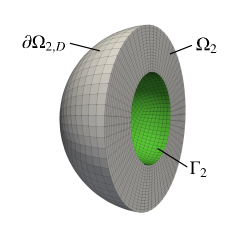
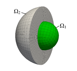
Figure 4: Slave (left) and master (center) domains. In green the interface $\Gamma$.

As FOM dimension, we consider $N=3474$ in the slave domain $\Omega_{1}$ and $N=26146$ in the master domains $\Omega_{2}$. We choose to vary the parameters $\alpha$ and $\beta$ in $[1,10]$ using a LHS to compute the solution snapshots. We select $N_{\text{train}}=150$ to get a sufficiently rich snapshots set to build the reduced bases, while additional $N_{\text{test}}=20$ values of the parameter vectors are chosen to test the method. Moreover, we prescribe for the stopping criteria of the Dirichlet-Neumann iteration a tolerance is $10^{-6}$. On average, FOM solution is found after 23 iterations for the coarser discretization and 24 iterations for the finer one, while ROM solution is found after 32 iterations.

$\alpha=2.35,~{}\beta=9.55$       $\alpha=6.85,~{}\beta=3.25$       $\alpha=4.15,~{}\beta=5.05$

                       

Figure 5: Slave solution FOM (top), ROM (center) solutions and absolute error (bottom) for three different parameter vectors.

$\alpha=2.35,~{}\beta=9.55$       $\alpha=6.85,~{}\beta=3.25$       $\alpha=4.15,~{}\beta=5.05$

Figure 6: Master solution FOM (top), ROM (center) solutions and absolute error (bottom) for three different parameter vectors.

                       

As highlighted in Section 2, Remark 3, for each set of parameters we solve twice the high-fidelity FOM (once with a conforming mesh on $\Omega$ designed starting from the mesh size in $\Omega_{1}$, and the other time with another conforming mesh on $\Omega$ designed starting from the mesh size in $\Omega_{2}$) and once the ROM. Computational errors are evaluated considering the difference between the FOM and ROM solutions in the $H^{1}(\Omega_{i})$ norm, i.e.

$$\|\mathbf{u}_{FOM}(\boldsymbol{\mu})-\mathbf{u}_{ROM}(\boldsymbol{\mu})\|_{H^{1}(\Omega_{i})},\quad i=1,2.$$ (3y)

Fig. 5.1 and 5.1 show three FOM and ROM solutions and the absolute error on the slave and the master domains, respectively, while in Fig. 5.1 we plot the 2-norm of the relative error for different dimensions of the ROM, i.e. for different values of the parameters $n_{1}$, $n_{2}$, $M_{1}$ and $M_{2}$ defined in Sections 3 and 4. After some tests, we chose to consider the same number of basis functions to get a fixed accuracy of the solution for the Dirichlet and Neumann data i.e. $M_{1}=M_{2}$, while we treat independently the number of basis functions $n_{1}$ and $n_{2}$ used for the master and slave reduction. Then, Fig. 5.1 shows an increase, even if small, of the solution accuracy when the number of basis functions of one of the reduced quantities involved in the procedure is increased, as expected from RB theory.

Figure 7: $H^{1}(\Omega_{i})$ mean error ($z$-axis) over the solution for $N_{\text{test}}$ different instances of the parameters between the FOM and ROM solutions varying the number of basis functions used to represent the slave and the master solution $n_{1}$ and $n_{2}$, and the interface data $M_{1}$ and $M_{2}$ ($x$- and $y$-axis). On the top row we fix the number of basis functions of the master problem to 5 (on the left) and to 7 for the slave problem (on the right), while on the bottom we fix to 6 the number of basis function for the interface data representation.

Table 1 compares the computational costs of solving problem (3x) with the proposed ROM rather than with the high-fidelity FOMs. In particular, the ROM is about 2.5 times faster than the FOM employing the coarser discretization, corresponding to a CPU time reduction of about 61%, while we are able to achieved a speed up of about 24 times compared to the FOM employing the finer discretization, corresponding to a reduction of 96% of the computational costs.

	# DoFs or # Basis				CPU time
	Master solution	Slave solution	Master interface	Slave interface	Online	Offline
FOM	3474	3474	386	386	$\sim$3.93$s$
	26146	26146	1538	1538	$\sim$37.16$s$
ROM	7	5	6	6	$\sim$1.55$s$	$\sim$1$h$45$m$

Table 1: High fidelity and reduced order model dimensions and CPU times. We highlight the performances of the ROM model with respect to FOM solution using colors from red (worst) to green (best).

5.2 Unsteady case: time-dependent heat equation

We now apply the proposed technique to a time-dependent problem. In particular, we consider the following initial-boundary value problem for the heat equation

$$\begin{cases}\displaystyle\frac{\partial u}{\partial t}-\nabla\cdot(\alpha\nabla u)=f&\text{in }\Omega\times(0,T)\\ \alpha\nabla u\cdot\mathbf{n}=0&\text{on }\partial\Omega\times(0,T)\\ u=0&\text{in }\Omega\times\{t=0\}\\ \end{cases}$$ (3ag)

being $\Omega=(-0.5,1.5)\times(-0.5,0.5)\times(-0.5,0.5)$ (see Figure 8) and

$$f=\begin{cases}1&\text{if }x<0\land 0.2<t<0.5\\ 0&\text{otherwise}.\end{cases}$$

The problem is parametrized through the coefficient $\alpha$ and – indirectly – through the time variable $t$.

To apply the reduced technique presented in this work, we split $\Omega$ in two cubes with a common plane $x=0.5$ that represents the interface $\Gamma$ (see Fig. 8). The application of Dirichlet-Neumann iterative scheme leads therefore to the two following sub-problems: given $\lambda_{2}^{0}$ on $\Gamma_{2}$, for each $k\geq 0$, solve until convergence of the interface solution

$$\begin{cases}\displaystyle\frac{\partial u_{1}^{k+1}}{\partial t}-\nabla\cdot(\alpha\nabla u_{1}^{k+1})=f&\text{in }\Omega_{1}\times(0,T)\\ \alpha\nabla u_{1}^{k+1}\cdot\mathbf{n}_{1}=0&\text{on }\partial\Omega_{1,N}\times(0,T)\\ u_{1}^{k+1}=\lambda_{2}^{k}&\text{on }\Gamma_{1}\times(0,T)\\ u_{1}^{k+1}=0&\text{in }\Omega_{1}\times\{t=0\}\end{cases}$$ (3ah)

and

$$\begin{cases}\displaystyle\frac{\partial u_{2}^{k+1}}{\partial t}-\nabla\cdot(\alpha\nabla u_{2}^{k+1})=f&\text{in }\Omega_{2}\times(0,T)\\ \alpha\nabla u_{2}^{k+1}\cdot\mathbf{n}_{2}=0&\text{on }\partial\Omega_{2,N}\times(0,T)\\ \alpha\nabla u_{2}^{k+1}\cdot\mathbf{n}_{2}=-\alpha\nabla u_{1}^{k+1}\cdot\mathbf{n}_{1}&\text{on }\Gamma_{2}\times(0,T)\\ u_{2}^{k+1}=0&\text{in }\Omega_{2}\times\{t=0\},\end{cases}$$ (3ai)

while

$$\lambda_{2}^{k+1}=\omega u_{2_{\Gamma_{2}}}^{k}-(1+\omega)\lambda_{2}^{k}.$$

As for the steady test case, a fixed point acceleration strategy with parameter $\omega=0.25$ is applied to accelerate the convergence of the Dirichlet-Neumann scheme for both FOM and ROM computations.

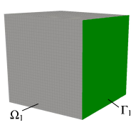
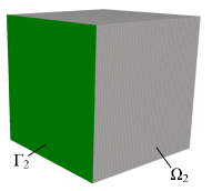
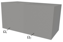
Figure 8: $\Omega_{1}$ (left) and $\Omega_{2}$ (center) and $\Omega$ (right). In green the interface $\Gamma$.

Two different discretizations corresponding to a FOM dimension equal to $N=35937$ for the slave domain and $N=274625$ DoFs for the master domain have been considered. The first order backward Euler scheme with $\Delta t=10^{-2}s$ has been used to handle time discretization. Moreover, the diffusive coefficients $\alpha$ is varied between 0.5 and 5, employing also in this case a LHS strategy to select the snapshots to be computed for the ROM training. In particular, we select $N_{S}=N_{t}N_{\text{train}}$ snapshots to train the ROM, corresponding to $N_{\text{train}}=$10 complete simulations in time, being $N_{t}=100$ the number of time steps in a model simulation. Then, $N_{\text{test}}=2$ simulations of 100 time steps each are considered to test the ROM. The tolerance to stop the Dirichlet-Neumann iteration is $10^{-6}$, which correspond to 18 iterations to find the FOM solution with the coarser discretization, 19 iterations for the FOM solution with the finer discretizations and 17 iterations to find the ROM solution for each time step.

$t=20s$            $t=40s$

Figure 9: Slave solution FOM (top), ROM (center) solutions and absolute error (bottom) for $\alpha=2.75$ and three different time instants.

                       

$t=20s$            $t=40s$

Figure 10: Master solution FOM (top), ROM (center) solutions and absolute error (bottom) for $\alpha=2.75$ and three different time instants.

                       

We compute the $H^{1}(\Omega_{i})$ error (3y) between the ROM and the coarse FOM solutions for the slave problem, and between the ROM and the fine FOM solutions for the master problem. In Figs. 5.2 and 5.2 we draw the ROM and FOM solutions and the absolute errors for three different time instants and some selected values of $\alpha$, while in Fig. 5.2 we plot the $H^{1}(\Omega_{i})$ error for different ROM dimensions. Note that fixing the number of basis functions used for both the slave solution, the master solution, and the interface Dirichlet-Neumann data, we show that the slave and master computational error decrease when increasing the number of basis functions, as expected.

Figure 11: $H^{1}(\Omega_{i})$ mean error ($z$-axis) over the solution for $N_{t}N_{\text{test}}$ different instances of the parameters between the FOM and ROM solutions varying the number of basis functions used to represent the slave and the master solution, and the interface data ($x$- and $y$-axis). On the top row we fix the number of basis functions of the master problem to 10 (on the left) and to 10 for the slave problem (on the right), while on the bottom we fix to 10 the number of basis function for the interface data representation.

Finally, in Table 2 we compare the computational costs of solving the problem with the FOM and the ROM. As before, our reduced technique shows high CPU performances, effectively achieving a speed up of 6.5 times with respect to the FOM solution with the coarsest discretization and of about 55.7 times compared to the finest discretization, corresponding a reduction of about 85% and 98% of the computational costs, respectively. These results refer to a complete simulation of 100 time steps, including some repeated tasks such as the assembling of the right-hand side, according to the time discretization scheme implemented. A hyper-reduction technique can be eventually included to enhance the online performance of the ROM even more.

	# DoFs or # Basis				CPU time
	Master solution	Slave solution	Master interface	Slave interface	Online	Offline
FOM	35937	35937	1089	1089	$\sim$36$m$ 6$s$
	274625	274625	4225	4225	$\sim$5$h$ 8$m$
ROM	10	10	10	10	$\sim$5m 32$s$	$\sim$8$h$

Table 2: FOM and ROM dimensions and CPU times. We highlight the ROM performances with respect to the ones of the FOM using colors from red (worst) to green (best).

6 Conclusion

In this work we have introduced a reduced order modeling technique based on RB methods to decrease the computational costs entailed by the solution of two-way coupled problems employing Dirichlet-Neumann iterative schemes. The modularity of the procedure ensures the efficiency of the ROM through different treatments of the master, slave and interface data reduction. Indeed, the master and the slave modes can be reduced using appropriate RB strategies, while the Dirichlet and the Neumann interface data can be handled through the DEIM inside the INTERNODES method, highlighting the possibility to use such reduced scheme to transmit the interface data between the conforming and non-conforming interface grids. The proposed algorithm can also be applied, in principle, to more general multi-physics problems that are solved through Dirichlet-Neumann domain-decomposition iterative schemes.

The numerical test cases show that our ROM is very cheap in the online phase, outperforming the online CPU time of the FOM when either fine or coarse conforming meshes in the two domains are considered. Indeed, a decrease of the 98% of the CPU time can be achieved in the case of a time-dependent parabolic PDE problem (see Subsection 5.2) with respect to a finite element FOM built over a fine discretization, and of the 85% with respect to a finite element FOM built over a coarser one.

This paper represents (at our knowledge) the first attempt towards the achievement of a fully-reduced RB interpolation based numerical scheme for two-way coupled model.

Future developments concern the use of the INTERNODES method on the FOM offline phase and the use of interpolation operators in the ROM online phase (see Remark 8) that are more accurate than those used in this paper. We are confident in this way to improve the accuracy as well as the efficiency (of the offline phase) of our approach. Finally, a future work will be the derivation of an error estimate for the proposed method.

Considering the results proposed in the last Section, we expect to be able to apply the presented method to more complex and relevant physics-based coupled problems, e.g. cardiac electrophysiological and fluid-structure interaction problems. Moreover, having been able to correctly reduce Dirichlet and Neumann interface data, the final extension of this work would be the application of our technique also to Robin-like interface conditions. All of these aspects will be the focus of future papers.

Statements and Declarations

This research has been funded partly by the European Research Council (ERC) under the European Union’s Horizon 2020 research and innovation programme (grant agreement No. 740132, iHEART “An Integrated Heart Model for the simulation of the cardiac function”, P.I. Prof. A. Quarteroni) and partly by the Italian Ministry of University and Research (MIUR) within the PRIN (Research projects of relevant national interest 2017 “Modeling the heart across the scales: from cardiac cells to the whole organ” Grant Registration number 2017AXL54F).

References

- Forti and Rozza [2014] D. Forti, G. Rozza, Efficient geometrical parametrisation techniques of interfaces for reduced-order modelling: application to fluid-structure interaction coupling problems, International Journal of Computational Fluid Dynamics 28 (2014) 158–169.
- Amsallem et al. [2010] D. Amsallem, J. Cortial, C. Farhat, Toward real-time computational-fluid-dynamics-based aeroelastic computations using a database of reduced-order information, AIAA Journal 48 (2010) 2029–2037.
- Ballarin et al. [2017] F. Ballarin, G. Rozza, Y. Maday, Reduced-order semi-implicit schemes for fluid-structure interaction problems, in: Model Reduction of Parametrized Systems, Springer, 2017, pp. 149–167.
- Ballarin and Rozza [2016] F. Ballarin, G. Rozza, Pod-galerkin monolithic reduced order models for parametrized fluid-structure interaction problems: Pod-galerkin monolithic rom for parametrized fsi problems, International Journal for Numerical Methods in Fluids 82 (2016).
- Lorenzi et al. [2016] S. Lorenzi, A. Cammi, L. Luzzi, G. Rozza, Pod-galerkin method for finite volume approximation of navier-stokes and rans equations, Computer Methods in Applied Mechanics and Engineering 311 (2016).
- Noack et al. [2016] B. Noack, W. Stankiewicz, M. Morzyński, P. Schmid, Recursive dynamic mode decomposition of transient and post-transient wake flows, Journal of Fluid Mechanics 809 (2016) 843–872.
- Ballarin et al. [2016] F. Ballarin, E. Faggiano, S. Ippolito, A. Manzoni, A. Quarteroni, G. Rozza, R. Scrofani, Fast simulations of patient-specific haemodynamics of coronary artery bypass grafts based on a POD-Galerkin method and a vascular shape parametrization, Journal of Computational Physics 315 (2016) 609–628.
- Fresca et al. [2021] S. Fresca, A. Manzoni, L. Dede, A. Quarteroni, Pod-enhanced deep learning-based reduced order models for the real-time simulation of cardiac electrophysiology in the left atrium, Frontiers in Physiology 12 (2021).
- Pagani et al. [2018] S. Pagani, A. Manzoni, A. Quarteroni, Numerical approximation of parametrized problems in cardiac electrophysiology by a local reduced basis method, Computer Methods in Applied Mechanics and Engineering 340 (2018).
- Schwarz [1869] H. Schwarz, Ueber einige abbildungsaufgaben, für die reine und angewandte Mathematik (1869) 105–120.
- Quarteroni and Valli [1999] A. Quarteroni, A. Valli, Domain Decomposition Methods for Partial Differential Equations, Numerical Mathematics and Scientific Computation, Oxford University Press, 1999.
- Glowinski et al. [1983] R. Glowinski, Q. Dinh, J. Periaux, Domain decomposition methods for nonlinear problems in fluid dynamics, Computer Methods in Applied Mechanics and Engineering 40 (1983) 27–109.
- Paz et al. [2010] R. Paz, M. Storti, L. Dalcin, G. Rios, Domain decomposition methods in computational fluid dynamics, Computational Mechanics Research Trends (2010) 495–555.
- Confalonieri et al. [2013] F. Confalonieri, A. Corigliano, M. Dossi, M. Gornati, A domain decomposition technique applied to the solution of the coupled electro-mechanical problem, International Journal for Numerical Methods in Engineering 93 (2013) 137–159.
- Weilun et al. [1998] Q. Weilun, S. Evans, H. Hastings, Efficient integration of a realistic two-dimensional cardiac tissue model by domain decomposition, IEEE Transactions on Biomedical Engineering 45 (1998) 372–385.
- McGee and Padmanabhan [2005] W. McGee, S. Padmanabhan, Non-Conforming Finite Element Methods for Nonmatching Grids in Three Dimensions, volume 40, 2005, pp. 327–334. doi:10.1007/3-540-26825-1_32.
- Oliver et al. [2009] J. Oliver, S. Hartmann, J. Cante, R. Weyler, J. Hernández, A contact domain method for large deformation frictional contact problems. part 1: Theoretical basis, Computer methods in applied mechanics and engineering 198 (2009).
- Hartmann et al. [2009] S. Hartmann, J. Oliver, R. Weyler, J. Cante, J. Hernández, A contact domain method for large deformation frictional contact problems. part 2: Numerical aspects, Computer Methods in Applied Mechanics and Engineering 198 (2009) 2607–2631.
- de Boer et al. [2007] A. de Boer, A. van Zuijlen, H. Bijl, Review of coupling methods for non-matching meshes, Computer Methods in Applied Mechanics and Engineering 196 (2007) 1515–1525.
- Chan et al. [1996] T. Chan, B. Smith, J. Zou, Overlapping schwarz methods on unstructured meshes usingnon-matching coarse grids, Numerische Mathematik 73 (1996) 149–167.
- Bernardi et al. [2005] C. Bernardi, Y. Maday, F. Rapetti, Basics and some applications of the mortar element method, GAMM-Mitteilungen 28 (2005).
- Hesch et al. [2014] C. Hesch, A. Gil, A. Arranz Carreño, J. Bonet, P. Betsch, A mortar approach for fluid-structure interaction problems: Immersed strategies for deformable and rigid bodies, Computer Methods in Applied Mechanics and Engineering 278 (2014).
- Deparis et al. [2016] S. Deparis, D. Forti, P. Gervasio, A. Quarteroni, Internodes: an accurate interpolation-based method for coupling the galerkin solutions of pdes on subdomains featuring non-conforming interfaces, Computers & Fluids 141 (2016).
- Gervasio and Quarteroni [2018] P. Gervasio, A. Quarteroni, Analysis of the internodes method for non-conforming discretizations of elliptic equations, Computer Methods in Applied Mechanics and Engineering 334 (2018) 138–166.
- Gervasio and Quarteroni [2019] P. Gervasio, A. Quarteroni, The internodes method for non-conforming discretizations of pdes, Communications on Applied Mathematics and Computation 1 (2019) 361–401.
- Quarteroni et al. [2016] A. Quarteroni, T. Lassila, S. Rossi, R. Ruiz Baier, Integrated heart - coupling multiscale and multiphysics models for the simulation of the cardiac function, Computer Methods in Applied Mechanics and Engineering 314 (2016).
- Hesthaven et al. [2016] J. Hesthaven, G. Rozza, B. Stamm, Certified Reduced Basis Methods for Parametrized Partial Differential Equations, 2016. doi:10.1007/978-3-319-22470-1.
- Benner et al. [2017] P. Benner, M. Ohlberger, A. Cohen, K. Willcox, Model reduction and approximation: Theory and algorithms., Society for Industrial and Applied Mathematics, Philadelphia, PA, 2017. doi:10.1137/1.9781611974829.
- Lucia et al. [2003] D. Lucia, P. King, P. Beran, Reduced order modeling of a two-dimensional flow with moving shocks, Computers & Fluids 32 (2003) 917–938.
- Xiao et al. [2019] D. Xiao, C. Heaney, L. Mottet, R. Hu, D. Bistrian, E. Aristodemou, I. Navon, C. Pain, A domain decomposition non-intrusive reduced order model for turbulent flows, Computers & Fluids 182 (2019).
- Wicke et al. [2009] M. Wicke, M. Stanton, A. Treuille, Modular bases for fluid dynamics, ACM Trans. Graph. 28 (2009).
- Baiges et al. [2013] J. Baiges, R. Codina, S. Idelsohn, A domain decomposition strategy for reduced order models. application to the incompressible navier–stokes equations, Computer Methods in Applied Mechanics and Engineering 267 (2013) 23–42.
- Washabaugh et al. [2012] K. Washabaugh, D. Amsallem, M. Zahr, C. Farhat, Nonlinear model reduction for cfd problems using local reduced order bases, AIAA-2012-2686, AIAA Fluid Dynamics and Co-located Conferences and Exhibit (2012).
- Iapichino et al. [2012] L. Iapichino, A. Quarteroni, G. Rozza, A reduced basis hybrid method for the coupling of parametrized domains represented by fluidic networks, Computer Methods in Applied Mechanics and Engineering 221-222 (2012) 63–82.
- Martini et al. [2015] I. Martini, G. Rozza, B. Haasdonk, Reduced basis approximation and a-posteriori error estimation for the coupled stokes-darcy system, Advances in Computational Mathematics 41 (2015) 1131–1157.
- Pegolotti et al. [2021] L. Pegolotti, M. Pfaller, A. Marsden, S. Deparis, Model order reduction of flow based on a modular geometrical approximation of blood vessels, Computer Methods in Applied Mechanics and Engineering 380 (2021) 113762.
- Legresley and Alonso [2006] P. Legresley, J. Alonso, Application of proper orthogonal decomposition (pod) to design decomposition methods /, 2006.
- Kerfriden et al. [2013] P. Kerfriden, O. Goury, T. Rabczuk, S. Bordas, A partitioned model order reduction approach to rationalise computational expenses in nonlinear fracture mechanics, Computer Methods in Applied Mechanics and Engineering 256 (2013) 169–188.
- Corigliano et al. [2015] A. Corigliano, M. Dossi, S. Mariani, Model order reduction and domain decomposition strategies for the solution of the dynamic elastic–plastic structural problem, Computer Methods in Applied Mechanics and Engineering 290 (2015) 127–155.
- Antil et al. [2010] H. Antil, M. Heinkenschloss, R. Hoppe, D. Sorensen, Domain decomposition and model reduction for the numerical solution of pde constrained optimization problems with localized optimization variables, Computing and Visualization in Science 13 (2010) 249–264.
- Antil et al. [2011] H. Antil, M. Heinkenschloss, R. Hoppe, Domain decomposition and balanced truncation model reduction for shape optimization of the stokes system, Optimization Methods and Software 26 (2011) 643–669.
- Maier and Haasdonk [2014] I. Maier, B. Haasdonk, A dirichlet–neumann reduced basis method for homogeneous domain decomposition problems, Applied Numerical Mathematics 78 (2014) 31–48.
- Zappon et al. [2022] E. Zappon, A. Manzoni, A. Quarteroni, Efficient and certified solution of parametrized coupled problems through deim-based data projection across non-conforming interfaces, 2022. arXiv:abs/2203.09226.
- Bjørstad et al. [2018] P. E. Bjørstad, S. C. Brenner, L. Halpern, H. H. Kim, R. Kornhuber, T. Rahman, O. B. Widlund, Domain Decomposition Methods in Science and Engineering XXIV, Lecture Notes in Computational Science and Engineering, Springer, Cham, 2018.
- Gervasio and Quarteroni [2018] P. Gervasio, A. Quarteroni, Internodes for heterogeneous couplings, in: P. E. Bjørstad, S. C. Brenner, L. Halpern, H. H. Kim, R. Kornhuber, T. Rahman, O. B. Widlund (Eds.), Domain Decomposition Methods in Science and Engineering XXIV, Springer International Publishing, Cham, 2018, pp. 59--71.
- Quarteroni et al. [2016] A. Quarteroni, A. Manzoni, F. Negri, Reduced Basis Methods for Partial Differential Equations. An Introduction, Springer International Publishing, 2016. doi:10.1007/978-3-319-15431-2.
- Brauchli and Oden [1971] H. Brauchli, J. Oden, Conjugate approximation functions in finite-element analysis, Quart. Appl. Math. 29 (1971) 65--90.
- Mckay et al. [1979] M. Mckay, R. Beckman, W. Conover, A comparison of three methods for selecting vales of input variables in the analysis of output from a computer code, Technometrics 21 (1979) 239--245.
- Iman and Helton [2006] R. Iman, J. Helton, An investigation of uncertainty and sensitivity analysis techniques for computer-models, Risk Analysis 8 (2006) 71 -- 90.
- Barrault et al. [2004] M. Barrault, Y. Maday, N. C. Nguyen, A. T. Patera, An ‘empirical interpolation’ method: application to efficient reduced-basis discretization of partial differential equations, C. R. Math. Acad. Sci. Paris 339 (2004) 667--672.
- Chaturantabut and Sorensen [2009] S. Chaturantabut, D. C. Sorensen, Discrete empirical interpolation for nonlinear model reduction, in: Proceedings of the 48h IEEE Conference on Decision and Control (CDC) held jointly with 2009 28th Chinese Control Conference, 2009, pp. 4316--4321. doi:10.1109/CDC.2009.5400045.
- Chaturantabut and Sorensen [2010] S. Chaturantabut, D. C. Sorensen, Nonlinear model reduction via discrete empirical interpolation, SIAM Journal on Scientific Computing 32 (2010) 2737--2764.
- Grepl et al. [2007] M. Grepl, Y. Maday, N. Nguyen, A. Patera, Efficient reduced-basis treatment of nonaffine and nonlinear partial differential equations, ESAIM: Mathematical Modelling and Numerical Analysis 41 (2007).
- Maday et al. [2008] Y. Maday, N. Nguyen, A. Patera, G. S. H. Pau, A general multipurpose interpolation procedure: The magic points, Communications on Pure and Applied Analysis 8 (2008).
- Negri et al. [2015] F. Negri, A. Manzoni, D. Amsallem, Efficient model reduction of parametrized systems by matrix discrete empirical interpolation, Journal of Computational Physics 303 (2015) 431--454.
- Farhat et al. [2020] C. Farhat, S. Grimberg, A. Manzoni, A. Quarteroni, Computational bottlenecks for proms: precomputation and hyperreduction, in: P. Benner, S. Grivet-Talocia, A. Quarteroni, G. Rozza, W. Schilders, L. Silveira (Eds.), Snapshot-Based Methods and Algorithms, De Gruyter, 2020, pp. 181--244.
- Africa et al. [2022] P. C. Africa, R. Piersanti, M. Fedele, L. Dede, A. Quarteroni, Lifex--heart module: a high-performance simulator for the cardiac function Package 1: Fiber generation, arXiv preprint arXiv:2201.03303 (2022).
- Arndt et al. [2021] D. Arndt, W. Bangerth, B. Blais, M. Fehling, R. Gassmöller, T. Heister, L. Heltai, U. Köcher, M. Kronbichler, M. Maier, P. Munch, J.-P. Pelteret, S. Proell, K. Simon, B. Turcksin, D. Wells, J. Zhang, The deal.II library, version 9.3, Journal of Numerical Mathematics (2021).