Large-eddy simulation of turbulent separated and reattached flow in enlarged annular pipe

Abstract

This study performs a large-eddy simulation of turbulent separated and reattached flow in an enlarged annular pipe. A vortex ring is periodically shed from the sudden expansion part. A longitudinal vortex occurs around the vortex ring, making the flow three-dimensional. As a result, the vortex ring becomes unstable downstream and splits into small vortices. A tubular longitudinal vortex structure occurs downstream of the reattachment point near the wall surface on the inner pipe side. A low-frequency fluctuation occurs at each pipe diameter ratio. The smaller the pipe diameter ratio is, the more downstream the influences of small-scale vortices and low-frequency fluctuation on the flow field appear. The smaller the pipe diameter ratio, the slower the pressure recovery downstream from the reattachment point. The pressure recovery on the inner pipe side is delayed compared to the outer pipe side. Turbulence is maximum upstream of the reattachment point due to the small-scale vortices generated by the collapse of the vortex ring. This maximum value decreases as the pipe diameter ratio decreases. The smaller the pipe diameter ratio, the higher the turbulence downstream from the reattachment point.

Keywords Separation, Reattachment, Turbulent flow, Vortex, Annular pipe, Numerical simulation

1 Introduction

Separated and reattached flows occur in various fluid machines and heat exchangers, causing deterioration in performance and efficiency and vibration and noise. On the other hand, since the heat transfer performance is improved by the strong mixing action of the flow field, the separated flow is actively used. Many studies have been conducted to clarify the characteristics of such separated flows (Lane and Loehrke, 1980; Ota et al., 1981; Kiya and Sasaki, 1983; Ayukawa et al., 1985; Bruno et al., 2010; Sasaki and Kiya, 1991; Yanaoka and Ota, 1996b, a, c; Hussein et al., 2011; Oon et al., 2003, 2014; Cao et al., 2014; Hussein et al., 2016).

The flow in the annular pipe targeted in this study is the flow form seen in engineering application equipment such as heat exchangers, nuclear reactors, and combustion engines. Therefore, research on annular flow has been conducted. Chung et al. (2002) performed direct numerical simulations on turbulent flow in an annular channel and found that in fully developed turbulent flow, velocity and turbulence distributions near the wall differ between the inner and outer tube sides. Rouiss et al. (2009) clarified the effect of the heat flux ratio on the heat transfer characteristics in turbulent flow in the annular channel by changing the heat flux applied to the inner and outer pipes.

In an annular flow, a separated and reattached flow occurs due to rapid expansion or contraction of the flow channel. Hussein et al. (2011) experimentally investigated the heat transfer characteristics in an enlarged annular flow, and Oon et al. (2003, 2014) investigated them by numerical analysis. On the other hand, Hussein et al. (2016) investigated the heat transfer characteristics in an enlarged annular flow channel using a nanofluid as a working fluid. In this way, several studies have been conducted focusing on the heat transfer characteristics of the enlarged annular flow. On the other hand, the unsteady characteristics of the flow field have not been investigated in detail. In particular, the effect of the diameter ratio of the inner and outer pipes on the separated and reattached flow has not been sufficiently investigated. In actual equipment, annular tubes with various pipe diameter ratios are used. In addition, the distributions of velocity and turbulence in the separated and reattached flow observed in the enlarged annular flow channel is considered to be greatly affected by the pipe diameter ratio, as in the case of the turbulent flow in the fully developed annular flow channel.

In this study, we perform numerical analysis using the LES model for the turbulent separated and reattached flow in an enlarged annular pipe and clarify the influence of the pipe diameter ratio on the vortex structure and turbulence characteristics.

2 Numerical procedures

Figure 1 shows the flow configuration and coordinate system. The origin is on the center axis at the sudden expansion step, and the $x$-, $y$-, and $z$-axes are the streamwise, radial, and circumferential directions, respectively. The velocities in these directions are denoted as $u_{x}$, $u_{r}$, and $u_{\theta}$, respectively. The inner radius of the annular pipe is $r_{1}$, the outer radius upstream of the step is $r_{2}$, and the outer radius downstream of the step is $r_{3}$. The hydraulic diameter $D$ is defined as $D=4A/L$. Here, $A$ is the cross-section area of the flow channel at the inlet, and $L$ is defined as $L=2\pi(r_{1}+r_{2})$. In this study, we consider a turbulent flow field in an enlarged annular pipe with an expansion rate of $ER=2.0$, which is defined as $ER=(r_{3}-r_{1})/(r_{2}-r_{1})$.

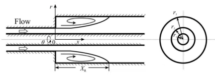
Figure 1: Flow configuration and coordinate system

This study deals with the three-dimensional flow of an incompressible viscous fluid with constant physical properties. The governing equations are the continuity and Navier-Stokes equations in a cylindrical coordinate system. These equations are non-dimensionalized using the hydraulic diameter $D$ and average velocity $U_{\mathrm{in}}$ at the inlet. The dimensionless governing equation is given as

$$\nabla\cdot{\bf u}=0,$$ (1)

$$\frac{\partial{\bf u}}{\partial t}+\nabla\cdot({\bf u}\otimes{\bf u})=-\nabla p+\frac{1}{Re}\nabla\cdot(2{\bf S}),$$ (2)

where the strain rate tensor is defined as

$${\bf S}=\frac{1}{2}[\nabla{\bf u}+(\nabla{\bf u})^{T}],$$ (3)

where coordinates and velocity vector are expressed as ${\bf x}=(x,r,\theta)$ and ${\bf u}=(u_{x},u_{r},u_{\theta})$, respectively. $t$ is time, $p$ is the pressure, $Re=U_{\mathrm{in}}D/\nu$ is the Reynolds number, and $\nu$ is the kinematic viscosity.

This study uses the dynamic SGS model (Germano et al., 1991; Lilly, 1992) as the LES model to analyze the turbulent field at a high Reynolds number. As a test filter, a top hat filter based on the trapezoidal rule is used (Najjar and Tafti, 1996), and the ratio of the test filter width to the grid filter width is $\sqrt{6}$.

The governing equations are solved using the simplified marker and cell method (Amsden and Harlow, 1970). The Crank-Nicolson method is applied to discretize the time derivative and then time marching is performed. The second-order central difference scheme is used to discretize the spatial derivative.

3 Calculation conditions

In this study, the inner radius of the annular pipe is set to be $r_{1}/D=0.15$, 0.3, and 0.5, and the outer radius upstream of the step is set to be $r_{2}/D=0.65$, 0.8, and 1.0. At that time, the pipe diameter ratios defined as $\alpha=r_{1}/r_{2}$ are $\alpha=0.23$, 0.375, and 0.5. We investigate the effect of changes in the diameter ratio on the flow field. The calculation area is from $x=-10D$ to $x=25D$ in the $x$-direction.

In turbulent flow analysis, it is a significant problem to give a turbulent inflow velocity at the inlet of a flow channel. This study generates a periodic flow in the calculation region from $x/D=-10$ to $x/D=-5.0$. At each time step, we use the velocity of the cross-section at $x/D=-5.0$ as the turbulent inflow velocity at the inlet of the annular pipe. At that time, we adjust the inflow velocity $u_{x}$ so that the flow rate at the inlet becomes constant. In addition, non-slip conditions are given on the wall surface, and convection boundary conditions are used at the outlet.

The time-averaged streamwise velocity distribution at the inlet is compared with the previously reported result (Chung et al., 2002) in Fig. 2 to validate the turbulent inflow velocity given at the inlet. Since this calculation result for $\alpha=0.5$ agrees well with the previous result, it can be seen that the turbulent flow is appropriately given in this calculation. Also, as in the previous study, when $\alpha$ becomes small, the peak of the distribution tends to be close to the inner pipe side of the annular pipe.

Three grids are used to confirm the dependency of the grids on the calculation results. The grid points of grid1, grid2, and grid3 are $254\times 50\times 58$, $311\times 84\times 61$, and $402\times 114\times 71$, respectively. The grid width is dense near the wall surface and the sudden expansion part. The minimum grid widths in grid1, grid2, and grid3 are $0.02D$, $0.01D$, and $0.005D$, respectively. We investigated the difference in calculation results depending on the number of grid points for $\alpha=0.5$, where the grid resolution in the circumferential direction is the coarsest among all the conditions. We will discuss the grid dependency later. In this study, to clarify the turbulence due to the vortex structure in more detail, the results using grid3 are mainly shown.

This study performs the calculation under the Reynolds number $Re=10^{4}$ defined by $D$ and $U_{\mathrm{in}}$. The time intervals used in the calculation are $\Delta t/(D/U_{\mathrm{in}})=0.01$, 0.005, and 0.0025 for grid1, grid2, and grid3, respectively. The dimensionless time to start sampling the data is $T=0$.

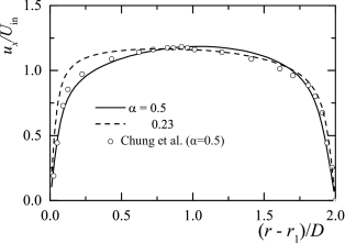
Figure 2: Time–averaged velocity distribution at inlet boundary

4 Results and discussion

4.1 Vortex structure

To clarify the vortex structure existing in the flow field, Fig. 3 to Fig. 5 show the isosurface of the curvature calculated from the equipressure surface. The reattachment point $X_{\mathrm{R}}$ is $X_{\mathrm{R}}=4.07D$ for $\alpha=0.5$, $X_{\mathrm{R}}=4.84$ for $\alpha=0.375$, and $X_{\mathrm{R}}=5.84D$ for $\alpha=0.23$. In all $\alpha$ values, the shear layer separated from the step of the sudden expansion step rolls up, forming a vortex ring periodically. This vortex ring has a deformed shape due to turbulence. The vortex ring becomes unstable downstream, and the vortex ring splits into small vortices around $x/D=3.0-4.0$ for $\alpha=0.5$, $x/D=3.5-4.5$ for $\alpha=0.375$, and $x/D=4.0-5.0$ for $\alpha=0.23$. Downstream from the reattachment point, a tubular vortex extending in the streamwise direction can be confirmed mainly over the region from the center of the flow channel to the wall surface on the inner pipe side. We can find from the above result that the smaller $\alpha$, the more downstream the deformation process of a series of vortices occurs.

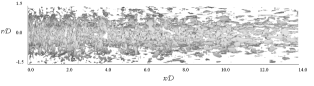
(a) Side view

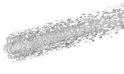
(b) Perspective view

Figure 3: Isosurface of curvature of equipressure surface at $T=0$ for $\alpha=0.5$: Isosurface value is $-27/D$.

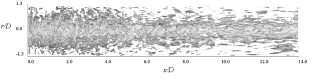
(a) Side view

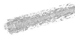
(b) Perspective view

Figure 4: Isosurface of curvature of equipressure surface at $T=0$ for $\alpha=0.375$: Isosurface value is $-27/D$.

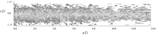
(a) Side view

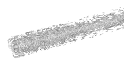
(b) Perspective view

Figure 5: Isosurface of curvature of equipressure surface at $T=0$ for $\alpha=0.23$: Isosurface value is $-27/D$.

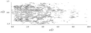
(a) Isosurface: Isosurface value is $\omega_{x}=5.0U_{\mathrm{in}}/D$.

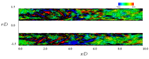
(b) Contour in $x$-$r$ plane: Contour interval is 0.5 from $-5.0$ to 5.0.

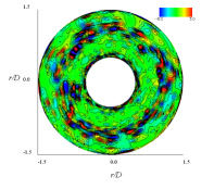
(c) Contour in $r$-$\theta$ plane at $x/D=1.5$: Contour interval is 0.5 from $-5.0$ to 5.0.

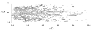
Figure 6: Streamwise vorticity for $\alpha=0.5$.

(a) Isosurface: Isosurface value is $\omega_{x}=5.0U_{\mathrm{in}}/D$.

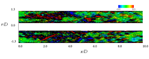
(b) Contour in $x$-$r$ plane: Contour interval is 0.5 from $-5.0$ to 5.0.

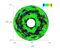
(c) Contour in $r$-$\theta$ plane at $x/D=1.5$: Contour interval is 0.5 from $-5.0$ to 5.0.

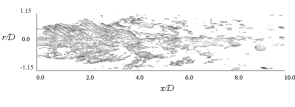
Figure 7: Streamwise vorticity for $\alpha=0.375$.

(a) Isosurface: Isosurface value is $\omega_{x}=5.0U_{\mathrm{in}}/D$.

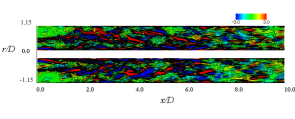
(b) Contour in $x$-$r$ plane: Contour interval is 0.5 from $-5.0$ to 5.0.

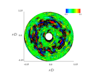
(c) Contour in $r$-$\theta$ plane at $x/D=1.5$: Contour interval is 0.5 from $-5.0$ to 5.0.

Figure 8: Streamwise vorticity for $\alpha=0.23$.

Next, we clarify the longitudinal vortex structure for each $\alpha$ value in detail. Figures 8 to 8 show the isosurface of the streamwise vorticity, the contour in the $x$-$r$ plane on the central axis, and the contour in the $r$-$\theta$ plane at $x/D=1.5$. Regardless of $\alpha$, many longitudinal vortex structures exist around the vortex ring generated by the rollup of the shear layer. This vortex is similar to the rib structure connecting strong lateral vortices lined up in a turbulent mixing layer. This longitudinal vortex strengthens the mixing of the flow and makes the flow three-dimensional. Therefore, the vortex ring becomes unstable, collapses, and splits into small-scale vortices downstream. In addition, we can confirm that the smaller $\alpha$ is, the stronger the longitudinal vortex structure exists downstream.

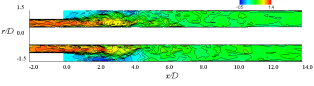
(a) Streamwise velocity contours: Contour interval is 0.1 from $-0.5$ to 1.4.

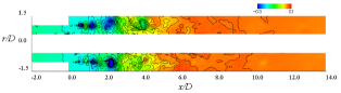
(b) Pressure contours: Contour interval is 0.02 from $-3.0$ to 0.1.

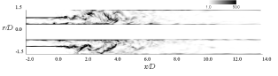
(c) Enstrophy contours

Figure 9: Instantaneous flow field in $x$-$r$ plane for $\alpha=0.5$.

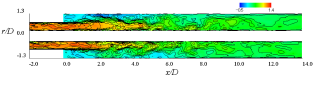
(a) Streamwise velocity contours: Contour interval is 0.1 from $-0.5$ to 1.4.

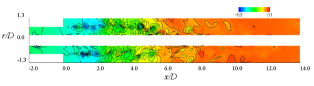
(b) Pressure contours: Contour interval is 0.02 from $-3.0$ to 0.1.

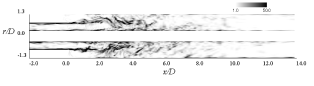
(c) Enstrophy contours

Figure 10: Instantaneous flow field in $x$-$r$ plane for $\alpha=0.375$.

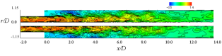
(a) Streamwise velocity contours: Contour interval is 0.1 from $-0.5$ to 1.4.

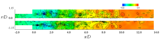
(b) Pressure contours: Contour interval is 0.02 from $-3.0$ to 0.1.

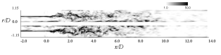
(c) Enstrophy contours

Figure 11: Instantaneous flow field in $x$-$r$ plane for $\alpha=0.23$.

Figures 11 to 11 show the streamwise velocity, pressure, and enstrophy distributions in the $x$-$r$ plane on the central axis for each $\alpha$ value. As seen in the streamwise velocity distribution, an asymmetric recirculation region is formed on the outer pipe side by the shear layer separated at the step. The high-speed fluid decelerates downstream and diffuses throughout the flow channel. The smaller $\alpha$, the longer the recirculation region becomes toward the downstream.

In the pressure distribution, just downstream of the sudden expansion part, the pressure drops due to the vortex ring generated by the rollup of the shear layer. We find that around the center of the shear layer at $(r-r_{1})/D=0.5$, high- and low-pressure changes are repeated alternately due to the vortex ring. Downstream, the vortex ring collapses, so the pressure change due to this vortex ring also disappears. The pressure is recovered in the redevelopment region downstream of the reattachment point. However, the small-scale vortex structure formed by the collapse of the vortex ring causes a local pressure drop mainly on the inner pipe side. The smaller $\alpha$ is, the more pronounced this pressure drop.

It can be seen from the enstrophy distribution that the flow separates at the step, and the separated shear layer extends downstream. The shear layer becomes unstable downstream and rolls up into a vortex, partly colliding with the wall surface on the outer pipe side, as seen near $x/D=2.0$ in the distribution of $\alpha=0.5$.

(a) $\alpha=0.5$

(b) $\alpha=0.375$

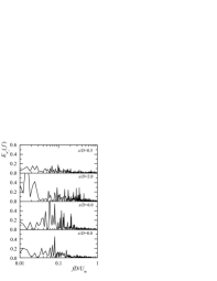
(c) $\alpha=0.23$

Figure 12: Power spectrums of streamwise velocity fluctuation at $(r-r_{1})/D=0.5$.

4.2 Frequency characteristics

Figure 12 shows the power spectrum of the streamwise velocity fluctuation $u_{x}^{\prime}$ at $(r-r_{1})/D=0.5$ near the center of the separated shear layer. At $x/D=2.0$, remarkable peaks for $\alpha=0.5$, 0.375, and 0.23 occur at $f=0.097U_{\mathrm{in}}/D$, $0.083U_{\mathrm{in}}/D$, and $0.091U_{\mathrm{in}}/D$, respectively. This is the shedding frequency of the vortex ring. In addition, regardless of $\alpha$, several peaks can be seen from $f=0.07U_{\mathrm{in}}/D$ to $f=0.4U_{\mathrm{in}}/D$ due to the disturbance from the upstream. Furthermore, for $\alpha=0.5$, 0.375, and 0.23, peaks occur around $f=0.021U_{\mathrm{in}}/D$, $0.027U_{\mathrm{in}}/D$, and $0.024U_{\mathrm{in}}/D$, respectively, on the low frequency side. This is considered to represent the low frequency fluctuation of the separated shear layer. Many peaks due to many small-scale vortices caused by the collapse of the vortex ring appear in the distributions at $x/D=4.0$ for $\alpha=0.5$, $x/D=5.0$ for $\alpha=0.375$, and $x/D=6.0$ for $\alpha=0.23$.

In this study, to clarify the spatiotemporal behavior of the vortex structure, we performed a wavelet transform, which is a kind of time-frequency analysis. The wavelet transform $W(a,b)$ is defined by the following equation by a signal $x(t)$ and the mother wavelet $\psi(t)$.

$$W(a,b)=\int_{-\infty}^{\infty}x(t)\psi_{a,b}^{*}(t)dt=\frac{1}{\sqrt{a}}\int_{-\infty}^{\infty}x(t)\psi^{*}\left(\frac{t-b}{a}\right)dt,$$ (4)

where $a$ and $b$ are parameters for scaling and translating the mother wavelet. This study selected the Mexican hat defined by the following equation for the mother wavelet.

$$\psi(t)=(1-t^{2})\exp\left(\frac{-t^{2}}{2}\right).$$ (5)

This wavelet is a real wavelet that shows good temporal resolution at sufficient frequency resolution and is suitable for the analysis of spatiotemporal behavior of large-scale vortex structures (Lee and Sung, 2001). Since the scaling parameter $a$ corresponds to the wavelet period, the relationship of $f\propto a^{-1}$ holds, and the relational expression between the scaling parameter and frequency in the Mexican hat is given as

$$f=\frac{\sqrt{5/2}}{2\pi a}.$$ (6)

Figure 13 shows the wavelet transform obtained by streamwise velocity fluctuation at $(r-r_{1})/D=0.5$. In the distribution of $x/D=2.0$, a striped pattern centered on $f=0.1U_{\mathrm{in}}/D$ at each $\alpha$ value appears periodically. This pattern represents the shedding of a vortex ring. In addition, low-frequency fluctuation of the separated shear layer occurs at the center of $f=0.03U_{\mathrm{in}}/D$ regardless of $\alpha$. Many striped patterns in the frequency band indicating the shedding of the vortex ring are present in the same time zone as the frequency band indicating the low-frequency fluctuation. Therefore, it is considered that the low-frequency fluctuation promotes the destabilization of the separated shear layer and the rollup of the shear layer into the vortex ring. In the distribution around the recirculation region, stripes appear periodically at a higher frequency than the shedding frequency of the vortex ring, regardless of $\alpha$. At these positions, small-scale vortex groups generated by the collapse of the vortex ring were confirmed, so it is considered that the striped pattern on the high-frequency side is due to the small-scale vortices. Since most of the striped patterns due to this vortex group exist at the same time zone as the striped pattern showing low-frequency fluctuation, it is considered that the vortex group is strongly affected by the low-frequency fluctuation. At $x/D=8.0$ downstream from the reattachment point, the smaller the $\alpha$, the stronger the striped pattern due to small-scale vortices and low-frequency fluctuations. Therefore, the smaller the $\alpha$ is, the more the effects of vortex groups and low-frequency fluctuations on the flow field appear further downstream.

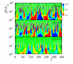
(a) $\alpha=0.5$

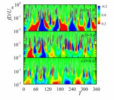
(b) $\alpha=0.375$

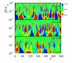
(c) $\alpha=0.23$

Figure 13: Wavelet transform of streamwise velocity fluctuation at $(r-r_{1})/D=0.5$.

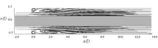
(a) Streamlines

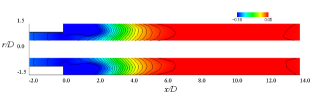
(b) Pressure contours: Contour interval is 0.01 from $-0.18$ to 0.05.

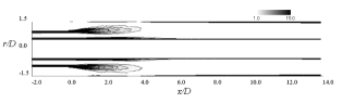
(c) Enstorophy contours: Contour interval is 1.0 from 1.0 to 15.0.

Figure 14: Time–averaged flow field in $x-r$ plane for $\alpha=0.5$.

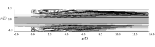
(a) Streamlines

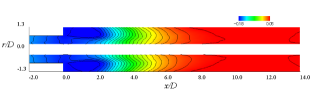
(b) Pressure contours: Contour interval is 0.01 from $-0.18$ to 0.05.

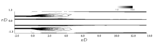
(c) Enstorophy contours: Contour interval is 1.0 from 1.0 to 15.0.

Figure 15: Time–averaged flow field in $x-r$ plane for $\alpha=0.375$.

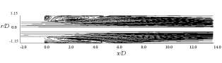
(a) Streamlines

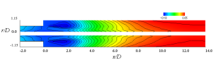
(b) Pressure contours: Contour interval is 0.01 from $-0.18$ to 0.05.

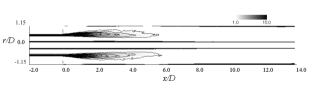
(c) Enstorophy contours: Contour interval is 1.0 from 1.0 to 15.0.

Figure 16: Time–averaged flow field in $x-r$ plane for $\alpha=0.23$.

(a) $C_{f}$

(b) $C_{p}$

Figure 17: Time–averaged distributions of surface friction coefficient and surface pressure coefficient: —, $\alpha=0.5$; - - -, $\alpha=0.375$; - $\cdot$ -, $\alpha=0.23$.

(a) $U_{x}/U_{\mathrm{in}}$

(b) $U_{r}/U_{\mathrm{in}}$

Figure 18: Time–averaged velocity distributions: —, $\alpha=0.5$; - - -, $\alpha=0.375$; - $\cdot$ -, $\alpha=0.23$.

4.3 Time-averaged flow field

Figures 16 to 16 show the time-averaged streamline, pressure, and enstrophy distributions for each $\alpha$ value. In the streamline distribution, regardless of $\alpha$, the flow separated at the step attaches to the outer pipe wall surface downstream, generating a separation bubble. Furthermore, a secondary vortex is formed on the outer pipe side just downstream of the step.

The pressure drops sharply because a vortex ring is shed at the step. Downstream, the vortex ring collapses and splits into small vortices, so the pressure rises around $x/D=3.5$ for $\alpha=0.5$, $x/D=4.0$ for $\alpha=0.375$, and $x/D=4.5$ for $\alpha=0.23$. Because the small-scale vortices decay downstream of the reattachment point, for $\alpha=0.5$, 0.375, and 0.23, the pressure becomes almost constant downstream from about $x/D=6.0$, 8.0, and 10.0, respectively. In addition, there is a region where the pressure recovery on the inner pipe side is delayed compared to the outer pipe side. This is because the small-scale vortex group generated by the collapse of the vortex ring is concentrated on the inner pipe side downstream, and a tubular longitudinal vortex structure is formed near the wall surface. The smaller $\alpha$, the more pronounced this tendency.

In the enstrophy distribution, the smaller $\alpha$ is, the more downstream the separated shear layer extends. Regardless of $\alpha$, the shear layer diffuses in the radial direction downstream, and the shear of the velocity decays.

Figure 17 shows the time-averaged distributions of surface friction coefficient $C_{f}$ and surface pressure coefficient $C_{p}$, which are averaged in the circumferential direction, on the outer pipe side. $C_{f}$ has a maximum value just downstream of the step because the recirculation of the flow generates a secondary vortex. $C_{f}$ decreased sharply downstream due to the rollup of the shear layer, and for $\alpha=0.5$, 0.375, and 0.23, $C_{f}$ becomes minimum at $x/D=2.3$, 2.6, and 2.9, respectively. This minimum indicates a strong reverse flow. Further downstream, $C_{f}$ increases sharply, reaches a maximum and then approaches a constant value. For $\alpha=0.5$, 0.375, and 0.23, $C_{p}$ becomes minimum at $x/D=1.3$, 1.36, and 1.65, respectively. Downstream, the pressure recovers sharply, and for $\alpha=0.5$, 0.375, and 0.23, $C_{p}$ gradually approaches a constant value around $x/D=7.0$, 9.0, and 11.0.

Figure 18 shows the time-averaged streamwise and radial velocity distributions, which are averaged in the circumferential direction. In Fig. 18 (a), reverse flow occurs on the outer pipe side downstream of the step, indicating the existence of a recirculation region. For all $\alpha$ values, the high-speed fluid ejected from the sudden expansion part decays downstream, and the velocity distribution becomes uniform. In addition, the velocity distribution for each $\alpha$ value just downstream of the step is almost the same near the inner pipe wall surface. However, the larger $\alpha$, the greater the deceleration in the vicinity of the inner pipe wall surface downstream. It is considered from this result that the larger $\alpha$, the stronger the influence of the inner pipe wall surface on the annular flow.

In Fig. 18 (b), the radial velocity is almost zero in the pipe upstream of the step. At $x/X_{\mathrm{R}}=0.2$ and 0.4, there are minimums inside the recirculation region. Upstream from the reattachment point of $x/X_{\mathrm{R}}\leq 1.0$, maximums induced by the vortex ring exist around $(r-r_{1})/D=0.5$. In addition, upstream of the reattachment point, the smaller $\alpha$, the slower the radial velocity.

(a) $k/U_{\mathrm{in}}^{2}$

(b) $u_{x,\mathrm{rms}}/U_{\mathrm{in}}$

(c) $u_{r,\mathrm{rms}}/U_{\mathrm{in}}$

(d) $u_{\theta,\mathrm{rms}}/U_{\mathrm{in}}$

Figure 19: Space–averaged distributions of turbulence kinetic energy and turbulence intensity of velocity fluctuation in $r-\theta$ plane.

(a) $u_{x,\mathrm{rms}}/U_{\mathrm{in}}$

(b) $u_{r,\mathrm{rms}}/U_{\mathrm{in}}$

(c) $u_{\theta,\mathrm{rms}}/U_{\mathrm{in}}$

(d) ${-u_{x}^{\prime}}{u_{r}^{\prime}}$

Figure 20: Turbulence intensity distributions of velocity fluctuations and Reynolds shear stress distributions: —, $\alpha=0.5$; - - -, $\alpha=0.375$; - $\cdot$ -, $\alpha=0.23$.

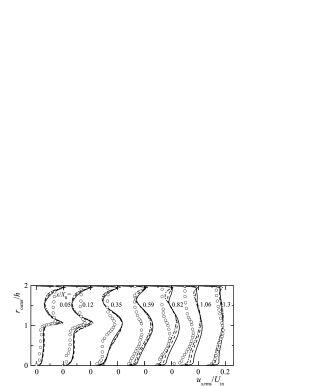
Figure 21: Turbulence intensity distributions of velocity fluctuations: —, $\alpha=0.5$; - - -, $\alpha=0.375$; - $\cdot$ -, $\alpha=0.23$; $\circ$, Yanhua et al. ($Re_{h}=3450$, $ER=1.01$).

(a) $u_{x,\mathrm{rms}}/U_{\mathrm{in}}$

(b) $u_{r,\mathrm{rms}}/U_{\mathrm{in}}$

(c) $u_{\theta,\mathrm{rms}}/U_{\mathrm{in}}$

(d) ${-u_{x}^{\prime}}{u_{r}^{\prime}}$

Figure 22: Turbulence intensity distributions of streamwise velocity, radial velocity, and circumferential velocity fluctuations, and Reynolds shear stress distribution for $\alpha=0.5$: - $\cdot$ -, grid1; - - -, grid2; —, grid3.

4.4 Turbulence characteristics

Figure 19 shows the turbulence kinetic energy $k$, the turbulence intensities of the streamwise velocity fluctuation $u_{x,\mathrm{rms}}$, radial velocity fluctuation $u_{r,\mathrm{rms}}$, and circumferential velocity fluctuation $u_{\theta,\mathrm{rms}}$. Each distribution was averaged over the $r-\theta$ cross-section. In the $k$ distribution shown in Fig. 19 (a), for $\alpha=0.5$, 0.375, and 0.23, the turbulence becomes maximum near $x/D=3.2$, 3.49, and 4.2, respectively, due to longitudinal vortices similar to the rib structure existing in the flow field and small-scale vortices generated by the collapse of the vortex ring. Downstream, the turbulence decreases as the small-scale vortex group decay. In addition, the smaller $\alpha$, the more downstream the small vortices concentrated on the inner pipe side exist, so $k$ shows a high value even downstream from the position of maximum turbulence. This trend is the same in the turbulence intensity distribution of each velocity fluctuation.

Figurea 20 (a) to (c) show the turbulence intensity distribution of each velocity fluctuation. In all distributions, maximums exist around the shear layer at $(r-r_{1})/D=0.5$ and near the inner pipe wall surface. We calculate the ratios of the maximum of $u_{r,\mathrm{rms}}$ and $u_{\theta,\mathrm{rms}}$ to $u_{x,\mathrm{rms}}$ around the separated shear layer at $x/X_{\mathrm{R}}=0.4$. The ratios are about 74% and 76% for $\alpha=0.5$, about 64% and 68% for $\alpha=0.375$, and about 55% and 67% for $\alpha=0.23$, respectively. Therefore, the flow has a strong three-dimensionality at this position because the longitudinal vortex existing around the vortex ring mixes the flow around the shear layer. Downstream, we can confirm that the turbulence of $0\leq(r-r_{1})/D\leq 0.5$ increases because the small-scale vortex group generated by the collapse of the vortex ring concentrates on the inner pipe side. In the Reynolds stress distribution ${-u_{x}^{\prime}}{u_{r}^{\prime}}$ shown in Fig.20 (d), regardless of $\alpha$, the magnitude of the extremum becomes maximum at $x/X_{\mathrm{R}}=0.6$ as in the $u_{x,\mathrm{rms}}$ distribution and attenuates downstream. The smaller $\alpha$, the smaller the extremum.

To show the validity of this calculation result, we compare the turbulence intensity distribution of the streamwise velocity fluctuation with the result of the three-dimensional backward step flow reported by Yanhua et al. (2013). In Fig. 21, $r_{\rm outer}=0$ is the outer pipe side wall surface, and $r_{\rm outer}=2h$ is the inner pipe side wall surface. Although $Re$ is different between this calculation and the experiment, the tendency that the maximum value due to the shear layer at $r_{\rm outer}=h$ gradually decreases toward the downstream is the same. In the present result, there is an extreme value near the wall surface due to the influence of the inner pipe wall surface. On the other hand, the maximum due to the wall surface cannot be seen near $r_{\rm outer}=2h$ in the experiment because the wall surface exists at about $r_{\rm outer}=80h$.

To confirm the dependency of the grid on the calculation result, we investigated the difference in the calculation result depending on the number of grid points for $\alpha=0.5$, where the grid resolution in the circumferential direction is the coarsest. Here, the distribution of turbulence averaged in the circumferential direction is shown. To evaluate the differences between the results obtained with grid1 and grid2 to grid3, we calculate the maximum difference mainly at the position where the distribution has a extreme value.

Figures 22 (a) to (c) show the turbulence intensity distribution of each velocity fluctuation. Overall, there is a difference upstream of $x/X_{\mathrm{R}}=0.4$. In the distribution of $u_{x,\mathrm{rms}}$, when comparing the maximum values around $(r-r_{1})/D=0.47$ at $x/X_{\mathrm{R}}=0.2$, the differences between the results of grid1 and grid2 to grid3 are about 6.7% and 0.14%, respectively. In the distribution of $u_{r,\mathrm{rms}}$, comparing the maximum values near $(r-r_{1})/D=0.5$ at $x/X_{\mathrm{R}}=0.4$, the differences between grid1 and grid2 to grid3 are about 6.5% and 0.19%, respectively. In the distribution of $u_{\theta,\mathrm{rms}}$, comparing the maximum values near $(r-r_{1})/D=0.5$ at $x/X_{\mathrm{R}}=0.2$, the differences between grid1 and grid2 to grid3 are about 10.7% and 2.1%, respectively. In the Reynolds stress distribution $-{u_{x}^{\prime}}{u_{r}^{\prime}}$ shown in Fig. 22 (d), there is a difference at $x/X_{\mathrm{R}}=0.2$. Comparing the maximum value near $(r-r_{1})/D=0.48$ at $x/X_{\mathrm{R}}=0.2$, the differences between the results of grid1 and grid2 to grid3 are about 17.3% and 2.1%, respectively. The difference between the results of grid2 and grid3 is small compared to the difference between the results of grid1 and grid2.

5 Conclusions

This study performed a large-eddy simulation of turbulent separated and reattached flow in an enlarged annular pipe. The obtained findings are summarized as follows.

At all the pipe diameter ratios, the shear layer separated from the sudden expansion part becomes unstable and rolls up into a vortex, shedding a vortex ring periodically. A longitudinal vortex similar to the rib structure occurs around the vortex ring, making the flow three-dimensional. As a result, the vortex ring becomes unstable downstream and splits into small vortices. A tubular longitudinal vortex structure occurs downstream of the reattachment point near the wall surface on the inner pipe side.

A low-frequency fluctuation occurs at each pipe diameter ratio. This low-frequency fluctuation can promote the destabilization of the vortex ring and its collapse. The smaller the pipe diameter ratio is, the more downstream the influences of small-scale vortices and low-frequency fluctuation on the flow field appear.

The smaller the pipe diameter ratio, the slower the pressure recovery downstream from the reattachment point. In addition, the pressure recovery on the inner pipe side is delayed compared to the outer pipe side due to the tubular longitudinal vortex structure and small-scale vortices existing near the inner pipe wall.

Regardless of the pipe diameter ratio, turbulence is maximum upstream of the reattachment point due to the small-scale vortices generated by the collapse of the vortex ring. This maximum value decreases as the pipe diameter ratio decreases. In addition, the smaller the pipe diameter ratio, the higher the turbulence downstream from the reattachment point.

Additional Information

Declaration of Interests: The authors report no conflict of interest.

Author contributions: H. Y. considered the content and policy of this research and constructed the calculation method and numerical codes. N. Y. performed the simulations. H. Y. and N. Y. contributed equally to analyzing data and reaching conclusions, and in writing the paper.

Author ORCID: H. Yanaoka https://orcid.org/0000-0002-4875-8174

References

- Amsden and Harlow (1970) Amsden, A.A., Harlow, F.H., 1970. A simplified MAC technique for incompressible fluid flow calculations. J. Comput. Phys. 6, 322–325. doi:doi:https://doi.org/10.1016/0021-9991(70)90029-X.
- Ayukawa et al. (1985) Ayukawa, K., Kawasaki, N., Ohkura, M., Asano, R., 1985. Rectangular cylinder in a shear flow. JSME, Ser.B 51, 3887–3895. doi:doi:https://doi.org/10.1299/kikaib.51.3887. (in Japanese).
- Bruno et al. (2010) Bruno, L., Fransos, D., Coste, N., Bosco, A., 2010. 3D flow around a rectangular cylinder: A computational study. J. Wind. Eng. Ind. Aerodyn. 98, 263–276. doi:doi:https://doi.org/10.1016/j.jweia.2009.10.005.
- Cao et al. (2014) Cao, S., Zhou, Q., , Zhou, Z., 2014. Velocity shear flow over rectangular cylinders with different side ratios. Comput. Fluids 96, 35–46. doi:doi:https://doi.org/10.1016/j.compfluid.2014.03.002.
- Chung et al. (2002) Chung, S.Y., Rhee, G.H., Sung, H.J., 2002. Direct numerical simulation of turbulent concentric annular pipe flow: Part 1: Fluid field. Int. J. Heat Fluid Flow 23, 426–440. doi:doi:https://doi.org/10.1016/S0142-727X(02)00140-6.
- Germano et al. (1991) Germano, M., Piomelli, U., Moin, P., Cabot, W.H., 1991. A dynamic subgrid-scale eddy viscosity model. Phys. Fluids A 3, 1760–1765. doi:doi:https://doi.org/10.1063/1.857955.
- Hussein et al. (2016) Hussein, T., Abu-Mulaweh, H.I., Kazi, S.N., Badarudin, A., 2016. Numerical simulation of heat transfer and separation Al2O3/nanofluid flow in concentric annular pipe. Int. Commun. Heat Mass Transf. 71, 108–117. doi:doi:https://doi.org/10.1016/j.icheatmasstransfer.2015.12.014.
- Hussein et al. (2011) Hussein, T., Salman, Y.K., Hakim, S.S.A., Kazi, S.N., 2011. An experimental study of heat transfer to turbulent separation fluid flow in an annular passage. Int. J. Heat Mass Transf. 54, 766–773. doi:doi:https://doi.org/10.1016/j.ijheatmasstransfer.2010.10.031.
- Kiya and Sasaki (1983) Kiya, M., Sasaki, K., 1983. Structure of a turbulent separation bubble. J. Fluid Mech. 137, 83–113. doi:doi:https://doi.org/10.1017/S002211208300230X.
- Lane and Loehrke (1980) Lane, J.C., Loehrke, R.I., 1980. Leading edge separation from a blunt plate at low Reynolds number. J. Fluid Eng. 102, 494–496. doi:doi:https://doi.org/10.1115/1.3240731.
- Lee and Sung (2001) Lee, I., Sung, H.J., 2001. Characteristics of wall pressure fluctuation in separated flows over a backward-facing step: Part II. unsteady wavelet analysis. Exp. Fluids 30, 273–28. doi:doi:https://doi.org/10.1007/s003480000173.
- Lilly (1992) Lilly, D.K., 1992. A proposed modification of the Germano subgrid-scale closure model. Phys. Fluids A 4, 633–635. doi:doi:https://doi.org/10.1063/1.858280.
- Najjar and Tafti (1996) Najjar, F.M., Tafti, D.K., 1996. Study of discrete test filters and finite difference approximations for the dynamic subgrid-scale stress model. Phys. Fluids 8, 1076–1088. doi:doi:https://doi.org/10.1063/1.868887.
- Oon et al. (2014) Oon, C.S., Al-Shamma‘a, A., Kazi, S.N., Chew, B.T., Badarudin, A., Sadeghinezhad, E., 2014. Simulation of heat transfer to separation air flow in a concentric pipe. Int. Commun. Heat Mass Transf. 57, 48–52. doi:doi:https://doi.org/10.1016/j.icheatmasstransfer.2014.07.008.
- Oon et al. (2003) Oon, C.S., Hussein, T., Kazi, S.N., Badarudin, A., Sadeghinezhad, E., 2003. Computational simulation of heat transfer to separation fluid flow in an annular passage. Int. Commun. Heat Mass Transf. 46, 92–96. doi:doi:https://doi.org/10.1016/j.icheatmasstransfer.2013.05.005.
- Ota et al. (1981) Ota, T., Asano, Y., Okawa, J., 1981. Reattachment length and transition of separated flow over blunt flat plates. Bull. JSME 94, 941–947. doi:doi:https://doi.org/10.1299/jsme1958.24.941.
- Rouiss et al. (2009) Rouiss, O.M., Saad, R.L., Lauriat, G., 2009. Direct numerical simulation of turbulent heat transfer in annuli: Effect of heat flux ratio. Int. J. Heat Fluid Flow 30, 579–589. doi:doi:https://doi.org/10.1016/j.ijheatfluidflow.2009.02.018.
- Sasaki and Kiya (1991) Sasaki, K., Kiya, M., 1991. Three-dimensional vortex structure in a leading-edge separation bubble at moderate Reynolds numbers. J. Fluids Eng. 113, 405–410. doi:doi:https://doi.org/10.1115/1.2909510.
- Yanaoka and Ota (1996a) Yanaoka, H., Ota, T., 1996a. Three-dimensional numerical simulation of laminar flow and heat transfer over blunt flat plate in a channel. JSME, Ser. B 62, 1496–1501. doi:doi:https://doi.org/10.1299/kikaib.62.1496. (in Japanese).
- Yanaoka and Ota (1996b) Yanaoka, H., Ota, T., 1996b. Three-dimensional numerical simulation of separated and reattached flow and heat transfer over blunt flat plate. JSME, Ser. B 62, 1111–1117. doi:doi:https://doi.org/10.1299/kikaib.62.1111. (in Japanese).
- Yanaoka and Ota (1996c) Yanaoka, H., Ota, T., 1996c. Three-dimensional numerical simulation of separated and reattached flow and heat transfer over blunt flat plate at high Reynolds number. JSME, Ser. B 62, 3439–3445. doi:doi:https://doi.org/10.1299/kikaib.62.3439. (in Japanese).
- Yanhua et al. (2013) Yanhua, W., Huiying, R., Hui, T., 2013. Turbulent flow over a rough backward–facing step. Int. J. Heat Fluid Flow 44, 155–169. doi:doi:https://doi.org/10.1016/j.ijheatfluidflow.2013.05.014.