Constrained Reinforcement Learning for Robotics
via Scenario-Based Programming

Abstract

Deep reinforcement learning (DRL) has achieved groundbreaking successes in a wide variety of robotic applications. A natural consequence is the adoption of this paradigm for safety-critical tasks, where human safety and expensive hardware can be involved. In this context, it is crucial to optimize the performance of DRL-based agents while providing guarantees about their behavior. This paper presents a novel technique for incorporating domain-expert knowledge into a constrained DRL training loop. Our technique exploits the scenario-based programming paradigm, which is designed to allow specifying such knowledge in a simple and intuitive way. We validated our method on the popular robotic mapless navigation problem, in simulation, and on the actual platform. Our experiments demonstrate that using our approach to leverage expert knowledge dramatically improves the safety and the performance of the agent.

Keywords: Robotic Navigation, Constrained Reinforcement Learning, Scenario Based Programming, Safety

1 Introduction

In recent years, deep neural networks (DNNs) have achieved state-of-the-art results in a large variety of tasks, including image recognition [1], game playing [2], protein folding [3], and more. In particular, deep reinforcement learning (DRL) [4] has emerged as a popular paradigm for training DNNs that perform complex tasks through continuous interaction with their environment. Indeed, DRL models have proven remarkably useful in robotic control tasks, such as navigation [5] and manipulation [6, 7], where they often outperform classical algorithms [8]. The success of DRL-based systems has naturally led to their integration as control policies in safety-critical tasks, such as autonomous driving [9], surgical assistance [10], flight control [11], and more. Consequently, the learning community has been seeking to create DRL-based controllers that simultaneously demonstrate high performance and high reliability; i.e., are able to perform their primary tasks while adhering to some prescribed properties, such as safety and robustness.

An emerging family of approaches for achieving these two goals, known as constrained DRL [12], attempts to simultaneously optimize two functions: the reward, which encodes the main objective of the task; and the cost, which represents the safety constraints. Current state-of-the-art algorithms include IPO [13], SOS [14], CPO [12], and Lagrangian approaches [15]. Despite their success in some applications, these methods generally suffer from significant setbacks: (i) there is no uniform and human-readable way of defining the required safety constraints; (ii) it is unclear how to encode these constraints as a signal for the training algorithm; and (iii) there is no clear method for balancing cost and reward during training, and thus there is a risk of producing sub-optimal policies.

In this paper, we present a novel approach for addressing these challenges, by enabling users to encode constraints into the DRL training loop in a simple yet powerful way. Our approach generates policies that strictly adhere to these user-defined constraints without compromising performance.

We achieve this by extending and integrating two approaches: the Lagrangian-PPO algorithm [15] for DRL training, and the scenario-based programming (SBP) [16, 17] framework for encoding user-defined constraints.

Scenario-based programming is a software engineering paradigm intended to allow engineers to create a complex system in a way that is aligned with how humans perceive that system. A scenario-based program is comprised of scenarios, each of which describes a single desirable (or undesirable) behavior of the system at hand; and these scenarios are then combined to run simultaneously, in order to produce cohesive system behavior. We show how such scenarios can be used to directly incorporate subject-matter-expert (SME) knowledge into the training process, thus forcing the resulting agent’s behavior to abide various safety, efficiency and predictability requirements.

In order to demonstrate the usefulness of our approach to robotic systems, we used it to train a policy for performing mapless navigation [18, 19] by the Robotis Turtlebot3 platform.

While common DRL-training techniques were shown to give rise to high-performance policies for this task [20], these policies are often unsafe, inefficient, or unpredictable, thus dramatically limiting their potential deployment in real-world systems [21, 14].

Our experiments demonstrate that, by using our novel approach and injecting subject-matter expert knowledge into the training process, we are able to generate trustworthy policies that are both safe and high performance. To have a complete assessment of the resulting behaviors, we performed a formal verification analysis [22, 23] of various predefined safety properties that proved that our approach generates safe agents to deploy in any environment.

2 Background

Deep Reinforcement Learning. Deep reinforcement learning [24] is a specific paradigm for training deep neural networks [25]. In DRL, the training objective is to find a policy that maximizes the expected cumulative discounted reward $R_{t}=\mathbb{E}\big{[}\sum_{t}\gamma^{t}\cdot r_{t}\big{]}$, where $\gamma\in\big{[}0,1\big{]}$ is the discount factor, a hyperparameter that controls the impact of past decisions on the total expected reward. The policy, denoted as $\pi_{\theta}$, is a probability distribution that depends on the parameters $\theta$ of the DNN, which maps an observed environment state $s$ to an action $a$. Proximal policy optimization (PPO) is a state-of-the-art DRL algorithm for producing $\pi_{\theta}$ [26]. A key characteristic of PPO is that it limits the gradient step size between two consecutive policy updates during training, to avoid changes that can drastically modify $\pi_{\theta}$ [27].

In mission-critical tasks, the concept of optimality often goes beyond the maximization of a reward, and also involves “hard” safety constraints that the agent must respect. A constrained markov decision process (CMDP) is an alternative framework for sequential decision making, which includes an additional signal: the cost function, defined as $C:\mathcal{S}\times\mathcal{A}\rightarrow\mathbb{R}$, whose expected values must remain below a given threshold $d\in\mathbb{R}$. CMDP can support multiple cost functions and their thresholds, denoted by $\{C_{k}\}$ and $\{d_{k}\}$, respectively. The set of valid policies for a CMDP is defined as:

$$\Pi_{\mathcal{C}}:=\{\pi_{\theta}\in\Pi:\ \forall k,\ J_{C_{k}}(\pi_{\theta})\leq d_{k}\}$$ (1)

where $J_{C_{k}}(\pi_{\theta})$ is the expected sum of the $k^{th}$ cost function over the trajectory and $d_{k}$ is the corresponding threshold. Intuitively, the objective is to find a policy function that respects the constraints (i.e., is valid) and which also maximizes the expected reward (i.e., is optimal). A natural way to encode constraints in a classical optimization problem is by using Lagrange multipliers. Specifically, in DRL, a possible approach is to transform the constrained problem into the corresponding dual unconstrained version [13, 12]. The optimization problem can then be encoded as follows:

$$J(\theta)=\min_{\pi_{\theta}}\max_{\lambda\geq 0}\mathcal{L}(\pi_{\theta},\lambda)=\min_{\pi_{\theta}}\max_{\lambda\geq 0}J_{R}(\pi_{\theta})-\sum_{K}\lambda_{k}(J_{C_{k}}(\pi_{\theta})-d_{k})$$ (2)

Crucially, the optimization of the function $J(\theta)$ can be carried out by applying any policy gradient algorithm, a common implementation is based on PPO [15].

Scenario-Based Programming. Scenario-based programming (SBP) [16, 28] is a paradigm designed to facilitate the development of reactive systems, by allowing engineers to program a system in a way that is close to how it is perceived by humans — with a focus on inter-object, system-wide behaviors. In SBP, a system is composed of scenarios, each describing a single, desired or undesired behavioral aspect of the system; and these scenarios are then executed in unison as a cohesive system.

An execution of a scenario-based (SB) program is formalized as a discrete sequence of events. At each time-step, the scenarios synchronize with each other to determine the next event to be triggered. Each scenario declares events that it requests and events that it blocks, corresponding to desirable and undesirable (forbidden) behaviors from its perspective; and also events that it passively waits-for. After making these declarations, the scenarios are temporarily suspended, and an event-selection mechanism triggers a single event that was requested by at least one scenario and blocked by none. Scenarios that requested or waited for the triggered event wake up, perform local actions, and then synchronize again; and the process is repeated ad infinitum. The resulting execution thus complies with the requirements and constraints of each of the individual scenarios [28, 17]. For a formal definition of SBP, see the paper from  Harel et al. [17].

Although SBP is implemented in many high-level languages, it is often convenient to think of scenarios as transition systems, where each state corresponds to a synchronization point, and each edge corresponds to an event that could be triggered.

Fig. 1 uses that representation to depict a simple SB program that controls the temperature and water-level in a water tank (borrowed from [29]). The scenarios add hot water and add cold water repeatedly wait for WATER LOW events, and then request three times the event Add HOT or Add COLD, respectively. Since these six events may be triggered in any order by the event selection mechanism, new scenario stability is added to keep the water temperature stable, achieved by alternately blocking Add HOT and Add COLD events.

The resulting execution trace is shown in the event log.

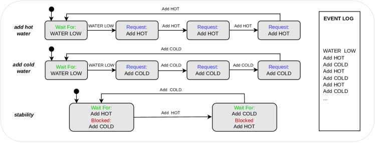
Figure 1: A scenario-based program for controlling a water tank. The small black circle indicates the initial state. The example is inspired by the work of Harel et al. [29].

A particularly useful trait of SBP is that the resulting models are amenable to model checking, and facilitate compositional verification [30, 31, 32, 33, 34]. Thus, it is often possible to apply formal verification to ensure that a scenario-based model satisfies various criteria, either as a stand-alone model or as a component within a larger system. Automated analysis techniques can also be used to execute scenario-based models in distributed architectures [35, 36, 37, 38, 39], to automatically repair these models [40, 29, 41], and to augment them in various ways, e.g., as part of the Wise Computing initiative [42, 43, 44]. In our context, SBP is an attractive choice for the incorporation of domain-specific knowledge into a DRL agent training process, due to being formal, fully executable and support of incremental development [45, 46, 47, 48, 49]. Moreover, the language it uses enables domain-specific experts to directly express their requirements specifications as an SB program.

Formal Verification of DNNs and DRL. A DNN verification algorithm receives the following inputs [22]: a trained DNN $N$, a precondition $P$ on the DNN’s inputs, and a postcondition $Q$ on $N$’s output. The precondition is used to limit the input assignments to inputs of interest, or to express some assumption the user has regarding the environment (e.g., that an image-recognition DNN will only be presented with certain pixel values). The postcondition typically encodes the negation of the behavior we would like $N$ to exhibit on inputs that satisfy $P$. Then, the verification algorithm searches for an input $x^{\prime}$ that satisfies the given conditions (i.e., $P(x^{\prime})\wedge Q(N(x^{\prime}))$), and returns exactly one of the following outputs: (i) SAT, indicating the query is satisfiable. Due to the postcondition $Q$ encoding the negation of the required property, this result indicates that the wanted property is violated in some cases. Modern verification engines also supply a concrete input $x^{\prime}$ that satisfies the query, and hence, a valid input that triggers a bug, such as an incorrect classification; or (ii) UNSAT, indicating that there does not exist such an $x^{\prime}$, and thus — that the desired property always holds.

Figure 2: A toy DNN.

For example, suppose we wish to guarantee that for all non-negative inputs $x=\langle v_{1}^{1},v_{1}^{2}\rangle$, the DNN in Fig. 2 always outputs a value strictly smaller than $40$; i.e., that that $N(x)=v_{4}^{1}<40$. This property can be encoded as a verification query consisting of a precondition that restrict the inputs to the desired range, i.e., $P=(v_{1}^{1}\geq 0)\wedge(v_{1}^{2}\geq 0)$, and by setting $Q=(v_{4}^{1}\geq 40)$, which is the negation of the desired property. In this case, a sound verifier will return SAT, alongside a feasible counterexample such as $x=\langle 2,3\rangle$, which produces the output $v_{4}^{1}=48\geq\ 40$ when fed to the DNN. Hence, the property does not always hold.

Originally, DNN verification engines were designed the verify the correct behaviour of feed-forward DNNs [22, 50, 51, 52, 53]. However, in recent years, the verification community has also designed verification methods tailored for DRL systems [7, 54, 55, 56, 57]. These methods include techniques for encoding multiple invocations of the agent in question, when interacting with a reactive environment over multiple time-steps.

Figure 3: The Robotis Turtlebot3 platform.

3 Expressing DRL Constraints using Scenarios

Mapless Navigation. We explain and demonstrate our proposed technique using the mapless navigation problem, in which a robot is required to reach a given target efficiently while avoiding collision with obstacles. Unlike in classical planning, the robot is not given a map of its surrounding environment and can rely only on local observations — e.g., from lidar sensors or cameras. Thus, a successful agent needs to be able to adjust its strategy dynamically, as it progresses towards its target. Mapless navigation has been studied extensively and is considered difficult to solve. Specifically, the local nature of the problem renders learning a successful policy extremely challenging and hard to solve using classical algorithms [58]. Prior work has shown DRL approaches to be among the most successful for tackling this task, often outperforming hand-crafted algorithms [20].

As a platform for our study, we used the Robotis Turtlebot 3 platform (Turtlebot, for short; see Fig. 3), which is widely used in the community [59, 60]. The Turtlebot is capable of horizontal navigation and is equipped with lidar sensors for detecting nearby obstacles. In order to train DRL policies for controlling the Turtlebot, we built a simulator based on the Unity3D engine [61], which is compatible with the Robotic Operating System (ROS) [62] and allows a fast transfer to the actual platform (sim-to-real [63]).

We used a hybrid reward function, which includes a discrete component for the terminal states (“collision”, or “reached target”), and a continuous component for the non-terminal states. Formally:

$$R_{t}=\begin{cases}\pm 1\hfill\text{terminal states}\\ (dist_{t-1}-dist_{t})\cdot\alpha-\beta\hskip 30.11249pt\text{otherwise}\\ \end{cases}$$ (3)

Where $dist_{k}$ is the distance from the target at time $k$; $\alpha$ is a normalization factor; and $\beta$ is a penalty, intended to encourage the robot to reach the target quickly (in our experiments, we empirically set $\alpha=3$ and $\beta=0.001$). Additionally, in terminal states, we increase the reward by $1$ if the target is reached, or decrease it by $1$ in case of collision.

For our DNN topology, we used an architecture that was shown to be successful in a similar setting [20]: (i) an input layer of nine neurons, including seven for the lidar scans and two for the polar coordinates of the target; (ii) two fully-connected hidden layers of 32 neurons each; and (iii) an output layer of three neurons for the discrete actions (i.e., move FORWARD, turn LEFT, and turn RIGHT).

In Section 4, we provide details about the training algorithm we used. Using the reward defined in Eq. 3, we were able to train agents that achieved high performance — i.e., obtained a success rate of approximately 95%, where “success” means that the robot reached its target without colliding into walls or obstacles.

Analyzing the trained agents further, we observed that even DRL agents that achieved a high success rate may demonstrate highly undesirable behavior in different scenarios. One such behavior is a sequence of back-and-forth turns, that causes the robot to waste time and energy. Another undesirable behavior is when the agent makes a lengthy sequence of right turns instead of a much shorter sequence of left turns (or vice versa), wasting time and energy. A third undesirable behavior that we observed is that the agent might decide not to move forward towards a target that is directly ahead, even when the path is clear. Our goal was thus to use our approach to remove these undesirable behaviors.

A Rule-Based Approach. Following the approach of [64], we integrated a scenario-based program into the DRL training process, in order to remove the aforementioned undesirable behaviors. More concretely, we created specific scenarios to rule out each of the three aforementioned undesirable behaviors we observed.

To accomplish this, we created a mapping between each possible action $a_{t}\in\{\text{Move {FORWARD}, Turn {LEFT}, Turn {RIGHT}}\}$ of the DRL agent and a dedicated event $e_{a_{t}}\in\{\text{SBP\_MoveForward, SBP\_TurnLeft, SBP\_TurnRight}\}$ within the scenario-based program. These events allow the various scenarios to keep track and react to the agent’s actions. Similarly to [64], we refer to these $e_{a_{t}}$ events as external events, indicating that they can only be triggered when requested from outside the SB program proper.

By convention, we assume that after each triggering of a single, external event, the scenario-based program executes a sequence of internal events (a super-step [64]), until it returns to a steady-state and then waits for another external event.

The novelty of our approach, compared to [64], is in the strategy by which we use scenarios to affect the training process. Specifically, we define the DRL cost function to correspond to violations of scenario constraints by the DRL agent. Whenever the agent selects an action that is mapped to a blocked SBP event, we increase the cost. This approach is described further in Section 4, and constitutes a general method for injecting explicit constraints (expressed, e.g., by scenarios) directly into the policy optimization process.

Example: Constraint Scenarios. Considering again our Turtlebot mapless navigation case study, we created scenarios for discouraging the three undesirable behaviors we had previously observed. The scenarios are visualized in Fig. 4, using an amalgamation of Statecharts and SBP graphical notation languages [65, 66].

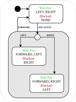
((a)) avoid back-and-forth rotation

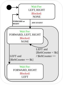
((b)) avoid turns larger than 180^∘

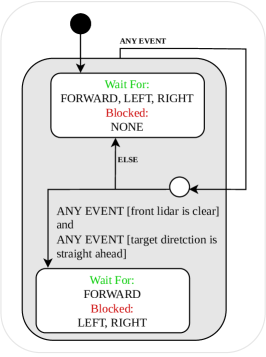
((c)) avoid turning when clear

Figure 4: A visualization of the three scenarios. Figure (b) refers to the Left turns part only. “Wait For” and “Blocked” in the state-blob indicates events that the scenario waits for or blocks, respectively. The events SBP_MoveForward, SBP_TurnLeft and SBP_TurnRight are represented respectively, by FORWARD, LEFT, RIGHT.

Scenario avoid back-and-forth rotation (Fig. 4(a)) seeks to prevent in-place, back-and-forth turns by the robot, to conserve time and energy.

Scenario avoid turns larger than 180^∘ (Fig. 4(b)) seeks to prevent left turns in angles that are greater than $180^{\circ}$, to conserve time and energy (the right-turn case is symmetrical). A forward slash indicates an action that is performed when a transition is taken; square brackets denote guard conditions, and $k and $leftCounter are variables. Each turn rotates the robot by $30^{\circ}$, and so we set $k=7$.

Scenario avoid turning when clear (Fig. 4(c)) seeks to force the agent to move towards the target when it is ahead, and there is a clear path to it. This is performed by blocking any turn actions when this situation occurs. Triggered events carry data, which can be referenced by guard conditions.

⬇

def SBP_avoidBackAndForthRotation():

blockedEvList = []

waitforEvList = [BEvent(”SBP_MoveForward”),

BEvent(”SBP_TurnLeft”),

BEvent(”SBP_TurnRight”)]

while True:

lastEv = yield {waitFor: waitforEvList, block: blockedEvList}

if lastEv != BEvent(”SBP_TurnLeft”)

and lastEv != BEvent(”SBP_TurnRight”):

blockedEvList = []

else:

blocked_ev = BEvent(”SBP_TurnRight”)

if lastEv == BEvent(”SBP_TurnLeft”)

else BEvent(”SBP_TurnLeft”)

# Blocking!

blockedEvList.append(blocked_ev)

Figure 5: The Python implementation of scenario avoid back-and-forth rotation. The code waits for any of the possible events: SBP_MoveForward, SBP_TurnLeft and SBP_TurnRight. Upon receiving SBP_TurnLeft, it blocks SBP_TurnRight, and upon receiving SBP_TurnRight, it blocks SBP_TurnLeft. Upon receiving SBP_MoveForward, it clears any blocking.

The Python implementation of avoid back-and-forth rotation is presented in Fig. 5, while a complete listing of all three scenarios appears in Appendix  A.

4 Using Scenarios in DRL Training

Even after defining constraints as an SB program, obtaining a differentiable function for the training process is not straightforward. We propose to use the following binary (indicator) function to this end:

$$c_{k}(s_{t},a,s_{t+1})=I(\text{the tuple }\langle s_{t},a,s_{t+1}\rangle\text{ is a blocked state in the SB program, by the $k^{th}$ rule})$$

Intuitively, summing the values of $c_{k}$ over a training episode yields the number of violations to the $k^{th}$ scenario rule during a single trajectory. This value can be treated as a cost function, the corresponding objective function defined as follows: $J_{C_{k}}=\sum_{I}c(s_{i},a_{i},s_{i+1})$, for a trajectory of $I$ steps. This value is dependent on the action policy $a$ and is therefore differentiable on the parameters $\theta$ of the policy through the policy gradient theorem.

Optimized Lagrangian-PPO. In Section 2 we proposed to relax the Lagrangian constrained optimization problem into an unconstrained, min-max version thereof. Taking the gradient of Equation 2, and some algebraic manipulation, we derive the following two simultaneous problems:

$$\nabla_{\theta}\mathcal{L}(\pi,\lambda)=\nabla_{\theta}(J_{R}(\pi)-\sum_{K}\lambda_{k}J_{C_{k}}(\pi))\hskip 30.11249pt\forall k,\hskip 10.03749pt\nabla_{\lambda_{k}}\mathcal{L}(\pi,\lambda)=-(J_{C_{k}}(\pi)-d_{k})$$ (4)

In closed form, the Lagrangian dual problem would produce exact results. However, when applied using a numerical method like gradient descent, it has shown strong instability and the proclivity to optimize only the cost, limiting the exploration and resulting in a poorly-performing agent [12]. To overcome these problems, we introduce three key optimizations that proved crucial to obtaining the results we present in the next section.

1. Reward Multiplier: the standard update rule for the policy in a Lagrangian method is given in Equation 4. However, as mentioned above, it often fails to maximize the reward. To overcome this failure, we introduce a new parameter $\alpha$, which we term reward multiplier, such that $\alpha\geq\sum_{K}\lambda_{k}$. This parameter is used as a multiplier for the reward objective:

   $$\nabla_{\theta}\mathcal{L}(\pi,\lambda)=\nabla_{\theta}(\alpha\cdot J_{R}(\pi)-\sum_{K}\lambda_{k}J_{C_{k}}(\pi))$$ (5)

2. Lambda Bounds and Normalization: Theoretically, the only constraint on the Lagrangian multipliers is that they be non-negative. However, when solving numerically, the value of $\lambda_{k}$ can increase quickly during the early stages of the training, causing the optimizer to focus primarily on the cost functions (Eq. 4), potentially not pushing the policy towards a high performance reward-wise. To overcome this, we introduced dynamic constraints on the multipliers (including the reward multiplier $\alpha$), such that $\sum_{K}\lambda_{k}+\alpha=1$. In order to also enforce the previously mentioned upper bound for $\alpha$, we clipped the values of the multipliers such that $\sum_{K}\lambda_{k}\leq\frac{1}{2}$. Formally, we perform the following normalization over all the multipliers:

   $$\forall k,\hskip 5.01874pt\lambda_{k}=\frac{\tilde{\lambda}_{k}}{2(\sum_{K}\tilde{\lambda}_{k})}\hskip 40.15pt\alpha=1-\sum_{K}\lambda_{k}$$ (6)

3. Algorithmic Implementation: the primary objective of the previously introduced optimizations is to balance the learning between the reward and the constraints. To further stabilize the training, we introduce additional, minor improvements to the algorithm: (i) lambda initialization: we initialize all the Lagrangian multipliers with zero to guarantee a focus on the reward optimization during the early stages of the training (consequently, following Eq. 6,  $\alpha=1$); (ii) lambda learning rate: to guarantee a smoother update of the Lagrangian multipliers, we scale this parameter to 10% of the learning rate used for the policy update; and (iii) delayed start: we enable the update of the multipliers only when the success rate is above 60% during the last 100 episodes. Intuitively, this delays the optimization of the cost functions until a minimum performance threshold is reached.

5 Evaluation

Setup. We performed training on a distributed cluster of HP EliteDesk machines, running at 3.00 GHz, with 32 GB RAM. We collected data from more than $100$ seeds for each algorithm, reporting the mean and standard deviation for each learning curve, following the guidelines of Colas et al. [67].

For training purposes, we built a realistic simulator based on the Unity3D engine [61]. Next, we evaluated the performance of the trained models using a physical Robotis Turtlebot3 robot (Fig. 3) and confirmed that it behaved similarly to the behavior observed in our simulations.

Results. Fig. 6 depicts a comparison between policies trained with a standard end-to-end PPO [26] (the baseline), and those trained using our constrained method with the injection of rules.

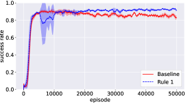
((a)) success rate

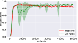
((b)) success rate

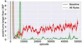
((c)) avoid turns larger than 180^∘

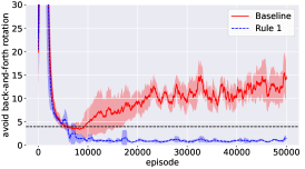
((d)) avoid back-and-forth rotation

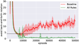
((e)) avoid back-and-forth rotation

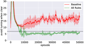
((f)) avoid turning when clear

Figure 6: A comparison between the baseline policies to policies trained using our approach. The black dotted line states the threshold ($d_{k}$) we considered for the $k^{th}$ rule.

In Figs. 6(a) and 6(d), we show results of policies trained with just avoid back-and-forth rotation added as a constraint.

Fig. 6(a) shows that the success rate of the baseline stabilizes at around $87\%$, while the success rate of our improved policies stabilizes at around $95\%$.

Fig. 6(d) then compares the frequency of undesired behavior occurrences between the baseline, at about $13$ per episode, and our policies, where the frequency diminishes almost completely.

Next, for Fig. 6(b) we show results of policies trained with all three of our added rules; we note that the success rate for these policies stabilizes around $95\%$, compared to $87\%$ for the baseline.

Finally, in Figs. 6(c), (e) and (f), we compare the frequency of the occurrence of undesired behaviors between the baseline and the policies trained with all rules active. Using the baseline, the frequency of the three behaviors is about $13$, $3$, and $17$ per episode. The undesired behaviors are removed almost completely for the policies trained with our additional rules and method.

We note that the undesired behavior addressed by the rule avoid turns larger than 180^∘ is quite rare in general; and so the statistics reported in Fig. 6(c) were collected over the final $100$ episodes of training.

The results clearly show that our method is able to train agents that respect the given constraints, without damaging the main training objective — the success rate. Moreover, it also highlights the scalability of our method, i.e., performing well when single or multiple rules are applied. Reviewing Fig 6(b), comparing the baseline’s success rate with our method’s success rate, when all rules are applied together with all the optimizations presented in Section 4, shows a clear advantage.

Excitingly, our approach even led to an improved success rate, suggesting that the contribution of expert knowledge can drive the training to better policies. This showcases the importance of enabling expert-knowledge contributions, compared to end-to-end approaches.

Formal Verification and Safety Guarantees. To further prove the effectiveness of our method, we show results of using the Marabou DNN verification engine [68, 69, 70, 71, 72, 73] to assess the reliability of our trained models. DNN verification is a sound and complete method for checking whether a DNN model displays unwanted behavior, over all possible inputs.

In order to conduct a fair comparison, we selected only models that passed our success cutoff value (85%); and for each of these models we ran three verification queries — each checking whether the model violates a given property (SAT), or abides by it for all inputs (UNSAT). We note that a verifier might also fail to terminate, due to TIMEOUT or MEMOUT errors. Each query ran with a TIMEOUT value of $36$ hours, and a MEMOUT value of $6$ GB. Table 1 summarizes the results of our experiments.

These results show a significant change of behavior between DNNs trained with the baseline algorithm, and those trained by our method. Indeed, we see that the latter policies much more often completely abide by the specific rules, and are consequently far more reliable.

Table 1: Results of the formal verification queries over a total of 120 trained DNNs, for each of the three properties in question. The first row shows the results of the 60 baseline policies, and the second row shows results of the 60 policies trained by our method, with all rules active.

	avoid back-and-forth rotation			avoid turns larger than 180∘			avoid turning when clear
ALGO	SAT	UNSAT	TIMEOUT	SAT	UNSAT	TIMEOUT	SAT	UNSAT	TIMEOUT
Baseline	60	0	0	51	0	9	60	0	0
SBP	22	38	0	0	41	19	9	34	17

6 Related Work

To the best of our knowledge, this is the first work that combines scenario-based programming into the training of a constrained reinforcement learning system — specifically in a robotic environment.

In [64], the authors proposed an integration between SBP and DRL training, using a reward shaping approach that penalizes the agent when rules are violated.

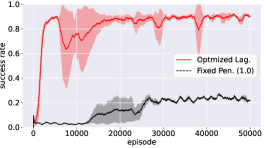
((a)) success rate

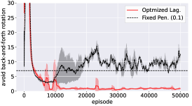
((b)) avoid back-and-forth rotation

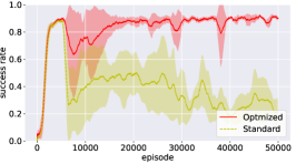
((c)) success rate

Figure 7: Graphs (a) and (b) show a comparison of our approach with that of [64]: graph (a) compares the success rates of the two approaches with all three scenario-based rules, and graph (b) compares the frequency of violations to the avoid back-and-forth rotation rule. For these two experiments, we configured the approach of [64] to use fixed penalties of $1.0$ and $0.05$, respectively. Graph (c) compares to the success rate of our approach to that of a policy trained with standard Lagrangian-PPO.

Our approach provides agents with fewer rule violations; parts (a) and (b) of Fig. 7 depict a comparison between our approach and that of Yerushalmi et al. [64], using different reward penalties to compare their effectiveness. Although the two approaches share some traits, their work requires us to manually determine the penalty that is incurred whenever the agent violates the scenario-based rules — which can be quite difficult [64]. Furthermore, this limitation renders the approach more difficult to apply incrementally: each additional scenario that is added to the SB program might require re-adjustments of the reward penalties, and this might become highly difficult for a large number of scenarios.

Constrained reinforcement learning is an emerging field [13, 14, 12]. To show the effectiveness of our approach, we also compared it to an implementation of Lagrangian-PPO, as suggested by [15]. The comparison results are shown in Fig. 7 (c). Although the technique of [15] is able to reduce the number of violations, it fails to reach a high success rate.

In a recent work on constrained reinforcement learning [74], the authors advocate an optimized version of Lagrangian-PPO. They propose a different approach to balance the constraints and the return, based on the softmax activation function and without imposing bounds on the values for the multipliers. Moreover, their work focuses on a different domain (game development), which presents very different challenges compared to robotics (e.g., safety and efficiency are not considered as crucial requirements); and they do not encode constraints using a framework geared for this purpose, such as SBP.

Limitations. Our method suffers from various limitations. First, it does not completely guarantee that the resulting policies are safe. For example, as shown in Table  1. Even though the number of formally safe models is significant, it is not absolute. In addition, using verification to check this may not always be feasible due to various limitations of current verification technology.

Second, our method requires prior knowledge of scenario-based programming to formalize the properties. To mitigate this, our approach can be extended to support additional rule-specifying formalisms, in addition to SBP. Third, the scalability of the method needs to be investigated. We showed in this work that the algorithm can easily handle one to three scenarios, in addition to the main objective. We leave to future work the analysis of performance when the number of properties increases further.

7 Conclusion

This paper presents a novel and generic approach for incorporating subject-matter-expert knowledge directly into the DRL learning process, allowing to achieve user-defined safety properties and behavioral requirements. We show how to encode the desired behavior as constraints for the DRL algorithm and improve a state-of-the-art algorithm with various optimizations. Importantly, we define properties comprehensibly, leveraging scenario-based programming to encode them into the training loop. We apply our method to a real-world robotic problem, namely mapless navigation, and show that our method can produce policies that respect all the constraints without adversely affecting the main objective of the optimization. We further demonstrate the effectiveness of our method by providing formal guarantees, using DNN verification, about the safety of trained policies.

Moving forward, we plan to extend our work to different environments including navigation in more complex domains (e.g., air and water). Another key challenge for the future is to inject rules aiming to encode behaviours in a cooperative (or competitive) multi-agent environment.

Appendix A SBP Python Objects Implementation

The Python implementation of the three scenarios used in this paper is shown below: the code for avoid back-and-forth rotation appears in Fig. 8, the code for avoid turns larger than 180^∘ appears in Fig. 9, and the code for avoid turning when clear appears in Fig. 10.

⬇

def SBP_avoidBackAndForthRotation():

blockedEvList = []

waitforEvList = [BEvent(”SBP_MoveForward”),

BEvent(”SBP_TurnLeft”),

BEvent(”SBP_TurnRight”)]

while True:

lastEv = yield {waitFor: waitforEvList, block: blockedEvList}

if lastEv != BEvent(”SBP_TurnLeft”)

and lastEv != BEvent(”SBP_TurnRight”):

blockedEvList = []

else:

blocked_ev = BEvent(”SBP_TurnRight”)

if lastEv == BEvent(”SBP_TurnLeft”)

else BEvent(”SBP_TurnLeft”)

# Blocking!

blockedEvList.append(blocked_ev)

Figure 8: The Python implementation of scenario avoid back-and-forth rotation. The code waits for any of the possible events: SBP_MoveForward, SBP_TurnLeft and SBP_TurnRight. Upon receiving SBP_TurnLeft, it blocks SBP_TurnRight, and upon receiving SBP_TurnRight, it blocks SBP_TurnLeft. Upon receiving SBP_MoveForward, it clears any blocking.

⬇

def SBP_avoid_k_consecuative_turns():

k = 7

counter = 0

prevEv = None

blockedEvList = []

waitforEvList = [BEvent(”SBP_MoveForward”), BEvent(”SBP_TurnLeft”), \\

BEvent(”SBP_TurnRight”)]

while True:

lastEv = yield {waitFor: waitforEvList, block: blockedEvList}

if prevEv is None or lastEv == BEvent(”SBP_MoveForward”) or prevEv != lastEv:

prevEv = lastEv

counter = 0

blockedEvList = []

else:

if counter == k - 1:

# Blocking!

blockedEvList.append(lastEv)

else:

counter += 1

Figure 9: The Python implementation of a scenario that blocks turning in the same direction more then k consecutive times. Each turn action rotates the robot by $30^{\circ}$, and so we set k to be 7.

⬇

def SBP_avoid_turning_when_clear():

blockedEvList = []

waitforEvList = [BEvent(”SBP_MoveForward”), BEvent(”SBP_TurnLeft”),\\

BEvent(”SBP_TurnRight”)]

while True:

lastEv = yield {waitFor: waitforEvList, block: blockedEvList}

state = lastEv.data[’state’]

if state[3] > MINIMAL_FWD_CLEARANCE and state[2] > MINIMAL_CLEARANCE and \\

state[4] > MINIMAL_CLEARANCE and abs(FWD_DIR - state[-2]) < FWD_DIR_TOLERANCE:

blockedEvList.extend([BEvent(”SBP_TurnLeft”), BEvent(”SBP_TurnRight”)])

else:

blockedEvList = []

Figure 10: The Python implementation of a scenario that blocks turning if the target is straight ahead and the path towards it is clear. The event carries data with it, which includes readings from the seven lidar sensors — with state[3] being the front-heading sensor. State[-2] is the direction to the target.

References

- Du [2018] J. Du. Understanding of Object Detection based on CNN Family and YOLO. Journal of Physics: Conference Series, 1004(1), 2018.
- Mnih et al. [2013] V. Mnih, K. Kavukcuoglu, D. Silver, A. Graves, I. Antonoglou, D. Wierstra, and M. Riedmiller. Playing Atari with Deep Reinforcement Learning, 2013. Technical Report. https://arxiv.org/abs/1312.5602.
- Jumper et al. [2021] J. Jumper, R. Evans, A. Pritzel, T. Green, M. Figurnov, O. Ronneberger, K. Tunyasuvunakool, R. Bates, A. Žídek, A. Potapenko, et al. Highly Accurate Protein Structure Prediction with AlphaFold. Nature, 2021.
- Sutton and Barto [2018] R. Sutton and A. Barto. Reinforcement Learning: An Introduction. MIT press, 2018.
- Kulhánek et al. [2019] J. Kulhánek, E. Derner, T. De Bruin, and R. Babuška. Vision-Based Navigation using Deep Reinforcement Learning. In Proc. 9th European Conf. on Mobile Robots (ECMR), pages 1–8, 2019.
- Nguyen and La [2019] H. Nguyen and H. La. Review of Deep Reinforcement Learning for Robot Manipulation. In Proc. 3rd IEEE Int. Conf. on Robotic Computing (IRC), pages 590–595, 2019.
- Corsi et al. [2021] D. Corsi, E. Marchesini, and A. Farinelli. Formal Verification of Neural Networks for Safety-Critical Tasks in Deep Reinforcement Learning. In Proc. 37th Conf. on Uncertainty in Artificial Intelligence (UAI), pages 333–343, 2021.
- Zhu and Zhang [2021] K. Zhu and T. Zhang. Deep Reinforcement Learning Based Mobile Robot Navigation: A Review. Tsinghua Science and Technology, 26(5):674–691, 2021.
- Sallab et al. [2017] A. Sallab, M. Abdou, E. Perot, and S. Yogamani. Deep Reinforcement Learning Framework for Autonomous Driving. Electronic Imaging, 19:70–76, 2017.
- Pore et al. [2021] A. Pore, D. Corsi, E. Marchesini, D. Dall’Alba, A. Casals, A. Farinelli, and P. Fiorini. Safe Reinforcement Learning using Formal Verification for Tissue Retraction in Autonomous Robotic-Assisted Surgery. In Proc. IEEE/RSJ Int. Conf. on Intelligent Robots and Systems (IROS), pages 4025–4031, 2021.
- Koch et al. [2019] W. Koch, R. Mancuso, R. West, and A. Bestavros. Reinforcement Learning for UAV Attitude Control. ACM Transactions on Cyber-Physical Systems, 3(2):1–21, 2019.
- Achiam et al. [2017] J. Achiam, D. Held, A. Tamar, and P. Abbeel. Constrained Policy Optimization. In Proc. 34th Int. Conf. on Machine Learning (ICML), pages 22–31, 2017.
- Liu et al. [2020] Y. Liu, J. Ding, and X. Liu. Ipo: Interior-Point Policy Optimization under Constraints. In Proc. 34th AAAI Conf. on Artificial Intelligence (AAAI), pages 4940–4947, 2020.
- Marchesini et al. [2021] E. Marchesini, D. Corsi, and A. Farinelli. Exploring Safer Behaviors for Deep Reinforcement Learning. In Proc. 35th AAAI Conf. on Artificial Intelligence (AAAI), 2021.
- Ray et al. [2019] A. Ray, J. Achiam, and D. Amodei. Benchmarking Safe Exploration in Deep Reinforcement Learning, 2019. Technical Report. https://cdn.openai.com/safexp-short.pdf.
- Damm and Harel [2001] W. Damm and D. Harel. LSCs: Breathing Life into Message Sequence Charts. Journal on Formal Methods in System Design (FMSD), 19(1):45–80, 2001.
- Harel et al. [2012] D. Harel, A. Marron, and G. Weiss. Behavioral Programming. Communications of the ACM (CACM), 55(7):90–100, 2012.
- Zhang et al. [2017] J. Zhang, J. Springenberg, J. Boedecker, and W. Burgard. Deep Reinforcement Learning with Successor Features for Navigation Across Similar Environments. In Proc. IEEE/RSJ Int. Conf. on Intelligent Robots and Systems (IROS), pages 2371–2378, 2017.
- Tai et al. [2017] L. Tai, G. Paolo, and . Liu. Virtual-to-Real Deep Reinforcement Learning: Continuous Control of Mobile Robots for Mapless Navigation. In Proc. IEEE/RSJ Int. Conf. on Intelligent Robots and Systems (IROS), pages 31–36, 2017.
- Marchesini and Farinelli [2020] E. Marchesini and A. Farinelli. Discrete Deep Reinforcement Learning for Mapless Navigation. In Proc. IEEE Int. Conf. on Robotics and Automation (ICRA), pages 10688–10694, 2020.
- Marchesini et al. [2021] E. Marchesini, D. Corsi, and A. Farinelli. Benchmarking Safe Deep Reinforcement Learning in Aquatic Navigation. In Proc. IEEE/RSJ Int. Conf on Intelligent Robots and Systems (IROS), 2021.
- Katz et al. [2017] G. Katz, C. Barrett, D. Dill, K. Julian, and M. Kochenderfer. Reluplex: An Efficient SMT Solver for Verifying Deep Neural Networks. In Proc. 29th Int. Conf. on Computer Aided Verification (CAV), pages 97–117, 2017.
- Liu et al. [2019] C. Liu, T. Arnon, C. Lazarus, C. Barrett, and M. Kochenderfer. Algorithms for Verifying Deep Neural Networks, 2019. Technical Report. http://arxiv.org/abs/1903.06758.
- Li [2017] Y. Li. Deep Reinforcement Learning: An Overview, 2017. Technical Report. http://arxiv.org/abs/1701.07274.
- Goodfellow et al. [2016] I. Goodfellow, Y. Bengio, and A. Courville. Deep Learning. MIT Press, 2016.
- Schulman et al. [2017] J. Schulman, F. Wolski, P. Dhariwal, A. Radford, and O. Klimov. Proximal Policy Optimization Algorithms, 2017. Technical Report. http://arxiv.org/abs/1707.06347.
- Schulman et al. [2015] J. Schulman, S. Levine, P. Abbeel, M. Jordan, and P. Moritz. Trust Region Policy Optimization. In Proc. 32nd Int. Conf. on Machine Learning (ICML), pages 1889–1897, 2015.
- Harel and Marelly [2003] D. Harel and R. Marelly. Come, Let’s Play: Scenario-Based Programming using LSCs and the Play-Engine, volume 1. Springer Science & Business Media, 2003.
- Harel et al. [2012] D. Harel, G. Katz, A. Marron, and G. Weiss. Non-Intrusive Repair of Reactive Programs. In Proc. 17th IEEE Int. Conf. on Engineering of Complex Computer Systems (ICECCS), pages 3–12, 2012.
- Harel et al. [2011] D. Harel, R. Lampert, A. Marron, and G. Weiss. Model-Checking Behavioral Programs. In Proc. 9th ACM Int. Conf. on Embedded Software (EMSOFT), pages 279–288, 2011.
- Harel et al. [2015] D. Harel, G. Katz, A. Marron, and G. Weiss. The Effect of Concurrent Programming Idioms on Verification. In Proc. 3rd Int. Conf. on Model-Driven Engineering and Software Development (MODELSWARD), pages 363–369, 2015.
- Katz et al. [2015] G. Katz, C. Barrett, and D. Harel. Theory-Aided Model Checking of Concurrent Transition Systems. In Proc. 15th Int. Conf. on Formal Methods in Computer-Aided Design (FMCAD), pages 81–88, 2015.
- Katz [2013] G. Katz. On Module-Based Abstraction and Repair of Behavioral Programs. In Proc. 19th Int. Conf. on Logic for Programming, Artificial Intelligence and Reasoning (LPAR), pages 518–535, 2013.
- Harel et al. [2015a] D. Harel, G. Katz, R. Lampert, A. Marron, and G. Weiss. On the Succinctness of Idioms for Concurrent Programming. In Proc. 26th Int. Conf. on Concurrency Theory (CONCUR), pages 85–99, 2015a.
- Harel et al. [2015b] D. Harel, A. Kantor, G. Katz, A. Marron, G. Weiss, and G. Wiener. Towards Behavioral Programming in Distributed Architectures. Journal of Science of Computer Programming (J. SCP), 98:233–267, 2015b.
- Steinberg et al. [2018] S. Steinberg, J. Greenyer, D. Gritzner, D. Harel, G. Katz, and A. Marron. Efficient Distributed Execution of Multi-Component Scenario-Based Models. Communications in Computer and Information Science (CCIS), 880:449–483, 2018.
- Steinberg et al. [2017] S. Steinberg, J. Greenyer, D. Gritzner, D. Harel, G. Katz, and A. Marron. Distributing Scenario-Based Models: A Replicate-and-Project Approach. In Proc. 5th Int. Conf. on Model-Driven Engineering and Software Development (MODELSWARD), pages 182–195, 2017.
- Greenyer et al. [2016] J. Greenyer, D. Gritzner, G. Katz, A. Marron, N. Glade, T. Gutjahr, and F. König. Distributed Execution of Scenario-Based Specifications of Structurally Dynamic Cyber-Physical Systems. In Proc. 3rd Int. Conf. on System-Integrated Intelligence: New Challenges for Product and Production Engineering (SYSINT), pages 552–559, 2016.
- Harel et al. [2013] D. Harel, A. Kantor, and G. Katz. Relaxing Synchronization Constraints in Behavioral Programs. In Proc. 19th Int. Conf. on Logic for Programming, Artificial Intelligence and Reasoning (LPAR), pages 355–372, 2013.
- Harel et al. [2014] D. Harel, G. Katz, A. Marron, and G. Weiss. Non-Intrusive Repair of Safety and Liveness Violations in Reactive Programs. Transactions on Computational Collective Intelligence (TCCI), 16:1–33, 2014.
- Katz [2021] G. Katz. Towards Repairing Scenario-Based Models with Rich Events. In Proc. 9th Int. Conf. on Model-Driven Engineering and Software Development (MODELSWARD), pages 362–372, 2021.
- Harel et al. [2018] D. Harel, G. Katz, R. Marelly, and A. Marron. Wise Computing: Toward Endowing System Development with Proactive Wisdom. IEEE Computer, 51(2):14–26, 2018.
- Harel et al. [2016a] D. Harel, G. Katz, R. Marelly, and A. Marron. An Initial Wise Development Environment for Behavioral Models. In Proc. 4th Int. Conf. on Model-Driven Engineering and Software Development (MODELSWARD), pages 600–612, 2016a.
- Harel et al. [2016b] D. Harel, G. Katz, R. Marelly, and A. Marron. First Steps Towards a Wise Development Environment for Behavioral Models. Int. Journal of Information System Modeling and Design (IJISMD), 7(3):1–22, 2016b.
- Gordon et al. [2012] M. Gordon, A. Marron, and O. Meerbaum-Salant. Spaghetti for the Main Course? Observations on the Naturalness of Scenario-Based Programming. In Proc. 17th ACM Annual Conf. on Innovation and Technology in Computer Science Education (ITCSE), pages 198–203, 2012.
- Alexandron et al. [2014] G. Alexandron, M. Armoni, M. Gordon, and D. Harel. Scenario-Based Programming: Reducing the Cognitive Load, Fostering Abstract Thinking. In Proc 36th Int. Conf. on Software Engineering (ICSE), pages 311–320, 2014.
- Katz and Elyasaf [2021] G. Katz and A. Elyasaf. Towards Combining Deep Learning, Verification, and Scenario-Based Programming. In Proc. 1st Workshop on Verification of Autonomous and Robotic Systems (VARS), pages 1–3, 2021.
- Katz [2021] G. Katz. Augmenting Deep Neural Networks with Scenario-Based Guard Rules. Communications in Computer and Information Science (CCIS), 1361:147–172, 2021.
- Katz [2020] G. Katz. Guarded Deep Learning using Scenario-Based Modeling. In Proc. 8th Int. Conf. on Model-Driven Engineering and Software Development (MODELSWARD), pages 126–136, 2020.
- Gehr et al. [2018] T. Gehr, M. Mirman, D. Drachsler-Cohen, E. Tsankov, S. Chaudhuri, and M. Vechev. AI2: Safety and Robustness Certification of Neural Networks with Abstract Interpretation. In Proc. 39th IEEE Symposium on Security and Privacy (S&P), 2018.
- Wang et al. [2018] S. Wang, K. Pei, J. Whitehouse, J. Yang, and S. Jana. Formal Security Analysis of Neural Networks using Symbolic Intervals. In Proc. 27th USENIX Security Symposium, pages 1599–1614, 2018.
- Lyu et al. [2020] Z. Lyu, C. Ko, Z. Kong, N. Wong, D. Lin, and L. Daniel. Fastened Crown: Tightened Neural Network Robustness Certificates. In Proc. 34th AAAI Conf. on Artificial Intelligence (AAAI), pages 5037–5044, 2020.
- Huang et al. [2017] X. Huang, M. Kwiatkowska, S. Wang, and M. Wu. Safety Verification of Deep Neural Networks. In Proc. 29th Int. Conf. on Computer Aided Verification (CAV), pages 3–29, 2017.
- Bacci et al. [2021] E. Bacci, M. Giacobbe, and D. Parker. Verifying Reinforcement Learning Up to Infinity. In Proc. 30th Int. Joint Conf. on Artificial Intelligence (IJCAI), 2021.
- Eliyahu et al. [2021] T. Eliyahu, Y. Kazak, G. Katz, and M. Schapira. Verifying Learning-Augmented Systems. In Proc. Conf. of the ACM Special Interest Group on Data Communication on the Applications, Technologies, Architectures, and Protocols for Computer Communication (SIGCOMM), pages 305–318, 2021.
- Amir et al. [2021] G. Amir, M. Schapira, and G. Katz. Towards Scalable Verification of Deep Reinforcement Learning. In Proc. 21st Int. Conf. on Formal Methods in Computer-Aided Design (FMCAD), pages 193–203, 2021.
- Amir et al. [2022] G. Amir, D. Corsi, R. Yerushalmi, L. Marzari, D. Harel, A. Farinelli, and G. Katz. Verifying Learning-Based Robotic Navigation Systems, 2022. Technical Report. https://arxiv.org/abs/2205.13536.
- Pfeiffer et al. [2018] M. Pfeiffer, S. Shukla, M. Turchetta, C. Cadena, A. Krause, R. Siegwart, and J. Nieto. Reinforced Imitation: Sample Efficient Deep Reinforcement Learning for Mapless Navigation by Leveraging Prior Demonstrations. IEEE Robotics and Automation Letters, 3(4):4423–4430, 2018.
- Nandkumar et al. [2021] C. Nandkumar, P. Shukla, and V. Varma. Simulation of Indoor Localization and Navigation of Turtlebot 3 using Real Time Object Detection. In Proc. Int. Conf. on Disruptive Technologies for Multi-Disciplinary Research and Applications (CENTCON), 2021.
- Amsters and Slaets [2019] R. Amsters and P. Slaets. Turtlebot 3 as a Robotics Education Platform. In Proc. 10th Int. Conf. on Robotics in Education (RiE), pages 170–181, 2019.
- Juliani et al. [2018] A. Juliani, V. Berges, E. Teng, A. Cohen, J. Harper, C. Elion, C. Goy, Y. Gao, H. Henry, M. Mattar, et al. Unity: A General Platform for Intelligent Agents, 2018. Technical Report. https://arxiv.org/abs/1809.02627.
- Quigley et al. [2009] M. Quigley, K. Conley, B. Gerkey, J. Faust, T. Foote, J. Leibs, R. Wheeler, et al. ROS: an Open-Source Robot Operating System. In Proc. ICRA Workshop on Open Source Software, 2009.
- Zhao et al. [2020] W. Zhao, J. Queralta, and T. Westerlund. Sim-To-Real Transfer in Deep Reinforcement Learning for Robotics: A Survey. In Proc. IEEE Symposium Series on Computational Intelligence (SSCI), pages 737–744, 2020.
- Yerushalmi et al. [2022] R. Yerushalmi, G. Amir, A. Elyasaf, D. Harel, G. Katz, and A. Marron. Scenario-Assisted Deep Reinforcement Learning. In Proc. 10th Int. Conf. on Model-Driven Engineering and Software Development (MODELSWARD), pages 310–319, 2022.
- Harel [1987] D. Harel. Statecharts: A Visual Formalism for Complex Systems. Science of Computer Programming, 8(3):231–274, 1987.
- Marron et al. [2018] A. Marron, Y. Hacohen, D. Harel, A. Mülder, and A. Terfloth. Embedding Scenario-based Modeling in Statecharts. In Proc. MoDELS Workshops, pages 443–452, 2018.
- Colas et al. [2019] C. Colas, O. Sigaud, and P. Oudeyer. A Hitchhiker’s Guide to Statistical Comparisons of Reinforcement Learning Algorithms, 2019. Technical Report. https://arxiv.org/abs/1904.06979.
- Katz et al. [2019] G. Katz, D. Huang, D. Ibeling, K. Julian, C. Lazarus, R. Lim, P. Shah, S. Thakoor, H. Wu, A. Zeljić, D. Dill, M. Kochenderfer, and C. Barrett. The Marabou Framework for Verification and Analysis of Deep Neural Networks. In Proc. 31st Int. Conf. on Computer Aided Verification (CAV), pages 443–452, 2019.
- Ostrovsky et al. [2022] M. Ostrovsky, C. Barrett, and G. Katz. An Abstraction-Refinement Approach to Verifying Convolutional Neural Networks, 2022. Technical Report. https://arxiv.org/abs/2201.01978.
- Wu et al. [2022] H. Wu, A. Zeljić, K. Katz, and C. Barrett. Efficient Neural Network Analysis with Sum-of-Infeasibilities. In Proc. 28th Int. Conf. on Tools and Algorithms for the Construction and Analysis of Systems (TACAS), pages 143–163, 2022.
- Strong et al. [2021] C. Strong, H. Wu, A. Zeljić, K. Julian, G. Katz, C. Barrett, and M. Kochenderfer. Global Optimization of Objective Functions Represented by ReLU Networks. Journal of Machine Learning, pages 1–28, 2021.
- Wu et al. [2020] H. Wu, A. Ozdemir, A. Zeljić, A. Irfan, K. Julian, D. Gopinath, S. Fouladi, G. Katz, C. Păsăreanu, and C. Barrett. Parallelization Techniques for Verifying Neural Networks. In Proc. 20th Int. Conf. on Formal Methods in Computer-Aided Design (FMCAD), pages 128–137, 2020.
- Amir et al. [2021] G. Amir, H. Wu, C. Barrett, and G. Katz. An SMT-Based Approach for Verifying Binarized Neural Networks. In Proc. 27th Int. Conf. on Tools and Algorithms for the Construction and Analysis of Systems (TACAS), pages 203–222, 2021.
- Roy et al. [2021] J. Roy, R. Girgis, J. Romoff, P. Bacon, and C. Pal. Direct Behavior Specification via Constrained Reinforcement Learning, 2021. Technical Report. https://arxiv.org/abs/2112.12228.