Compression and Data Similarity: Combination of Two Techniques for Communication-Efficient Solving of Distributed Variational Inequalities

Abstract

Variational inequalities are an important tool, which includes minimization, saddles, games, fixed-point problems. Modern large-scale and computationally expensive practical applications make distributed methods for solving these problems popular. Meanwhile, most distributed systems have a basic problem – a communication bottleneck. There are various techniques to deal with it. In particular, in this paper we consider a combination of two popular approaches: compression and data similarity. We show that this synergy can be more effective than each of the approaches separately in solving distributed smooth strongly monotone variational inequalities. Experiments confirm the theoretical conclusions.

1 Introduction

Variational inequalities are a broad class of problems that have been widely studied for a long time. This is primarily due to the uniqueness of variational inequalities; they can describe various types of optimization problems, which, in turn, have many practical applications [19, 7]. We can mention classic examples in economics and game theory [18], robust optimization [8], non-smooth optimization [39, 37], matrix factorization [6], image denoising [17, 13], supervised learning [5]. In recent years, there has been a significant increase in research interest toward the study of variational inequalities due to new connections with GANs [22]. In particular, the authors of [16, 21, 35, 14, 34, 40] show that even if one considers the classical (in the variational inequalities literature) regime involving monotone and strongly monotone inequalities, it is possible to obtain insights, methods and recommendations useful for the GANs training.

Until recently, theoretical studies of methods for variational inequalities were carried out only in the non-distributed setting. The Extra Gradient / Mirror Prox method [30, 38, 27] became widely known and very popular. This alorithm for variational inequalities is key and basic (as Gradient Descent for minimization problems). But new practical problems have opened up new challenges. Indeed, the training of modern supervised machine learning models in general, and deep neural networks in particular, becomes more and more demanding. Solving such problems is almost impossible without a distributed approach with parallelization [50].

Meanwhile, the distributed approach has its bottlenecks. The main one is communication cost, as the transfer of information between computing devices takes considerably longer than local processes. This is why it is important not just to get a distributed version of e.g. Extra Gradient [11], but a more effective method in terms of communication. The community already knows a number of approaches to communication efficient distributed optimization [29, 45, 20, 23]. For example, two such popular approaches are the compression of transmitted information, and the use of statistical similarity of local data on workers (if we spread the data uniformly among them).

Our contribution and related works. In this work we have combined two techniques for effective communications: compression and data similarity. Through this synthesis, we have obtained a method for distributed variational inequalities with better theoretical guarantees on the number of information transferred. See Table 1.

Table 1: Summary of complexities on the number of transmitted information for different approaches to communication bottleneck.
Notation: $\mu$ = constant of strong monotonicity of the operator $F$, $L$ = Lipschitz constant of the operator $F$, $\delta$ = similarity (relatedness) constant (Assumption 3), $M$ = number of devices, $b$ = local data size, $\varepsilon$ = precision of the solution.

Method	Reference	Technique	Amount of information	If $\delta\sim\tfrac{L}{\sqrt{b}}$
Extra Gradient	[27, 11]		$O\left(\frac{L}{\mu}\log\frac{1}{\varepsilon}\right)$	$O\left(\frac{L}{\mu}\log\frac{1}{\varepsilon}\right)$
SMMDS	[12]	similarity	$O\left(\frac{\delta}{\mu}\log\frac{1}{\varepsilon}\right)$	$O\left(\frac{1}{\sqrt{b}}\cdot\frac{L}{\mu}\log\frac{1}{\varepsilon}\right)$
MASHA	[10]	compression	$O\left(\frac{L}{\sqrt{M}\mu}\log\frac{1}{\varepsilon}\right)$	$O\left(\frac{1}{\sqrt{M}}\cdot\frac{L}{\mu}\log\frac{1}{\varepsilon}\right)$
Optimistic MASHA	This work	compression similarity	$O\left(\left[\frac{L}{M\mu}+\frac{\delta}{\sqrt{M}\mu}\right]\log\frac{1}{\varepsilon}\right)$	$O\left(\left[\frac{1}{M}+\frac{1}{\sqrt{Mb}}\right]\cdot\frac{L}{\mu}\log\frac{1}{\varepsilon}\right)$

Separately from each other, similarity and compression techniques have already been investigated for both particular minimization problems and general variational inequalities.

Different approaches with compression have been developed for minimization problems. Here we can highlight the earliest and the simplest approach, in which compression operators were applied to SGD-type methods [3]. Further modifications with ”memory” were presented in [36, 25]. Then accelerated methods were introduced by authors of [33]. The work [23] was tried to look at compression through the variance reduction technique. There is now widespread research into practical modifications with biased operators and error compensation [28, 53, 9, 43], bidirectional compression [47, 41], partial participation [26, 41, 23], etc. In the generality of variational inequalities, compression methods were studied in [10]. One can note that our new method are ahead of MASHA from this paper (record results in terms of compression methods for variational inequalities at the moment).

The literature on distributed minimization problems under similarity (relatedness) assumption is also vast. The paper [4] established lower communication complexity bounds. The authors of [44] proposed the mirror-descent based algorithm with data preconditioning. This technique was further accelerated by the inexact damped Newton method [52], the Catalyst framework [42] and the heavy ball momentum [51]. Higher order methods employing preconditioning were studied in [15, 1, 48]. Not for minimizations, but for variational inequalities and saddles, the similarity (relatedness) setup was considered by [12, 31]. In some cases, our estimates can also outperform the results from these works.

2 Problem setup and assumptions

2.1 Variational inequality

We consider variational inequalities (VI) of the form

$$\text{Find}~{}~{}z^{*} \in\mathbb{R}^{d}~{}~{}\text{such that}~{}~{}\langle F(z^{*}),z-z^{*}\rangle+g(z)-g(z^{*})\geq 0,~{}~{}\forall z\in\mathbb{R}^{d},$$ (1)

where $F:\mathbb{R}^{d}\to\mathbb{R}^{d}$ is an operator, and $g:\mathbb{R}^{d}\to\mathbb{R}\cup\{+\infty\}$ is a proper lower semicontinuous convex function. We assume that $F$ is distributed across $M$ workers/devices:

$$F(z)\vcentcolon=\frac{1}{M}\sum\limits_{m=1}^{M}F_{m}(z),$$ (2)

where $F_{m}:\mathbb{R}^{d}\to\mathbb{R}^{d}$ for all $m\in\{1,2,\dots,M\}$.

2.2 Examples

To showcase the expressive power of the formalism (1), we now give a few examples of variational inequalities arising in machine learning.

Example 1 [Convex minimization]. Consider the composite minimization problem:

$$\min_{z\in\mathbb{R}^{d}}f(z)+g(z),$$ (3)

where $f$ is typically a main term, and $g$ is a regularizer or an indicator function (e.g., if we want to consider the problem on some set). If we put $F(z)\vcentcolon=\nabla f(z)$, then it can be proved that $z^{*}\in\operatorname{\mathrm{dom}}g$ is a solution for (1) if and only if $z^{*}\in\operatorname{\mathrm{dom}}g$ is a solution for (3).

Example 2 [Convex-concave saddle point problems]. Consider the convex-concave saddle point problem

$$\min_{x\in\mathbb{R}^{d_{x}}}\min_{y\in\mathbb{R}^{d_{y}}}f(x,y)+g_{1}(x)+g_{2}(y),$$ (4)

where $g_{1}$ and $g_{2}$ can also be interpreted as regularizers or indicators. If we put $F(z)\vcentcolon=F(x,y)=[\nabla_{x}f(x,y),-\nabla_{y}f(x,y)]$ and $g(z)=g(x,y)=g_{1}(x)+g_{2}(y)$, then it can be proved that $z^{*}\in\operatorname{\mathrm{dom}}g$ is a solution for (1) if and only if $z^{*}\in\operatorname{\mathrm{dom}}g$ is a solution for (4).

While minimization problems are widely investigated separately from variational inequalities, saddles are very often studied together with variational inequalities. In particular, lower bounds for the former are also valid for the latter. Moreover, upper bounds for variational inequalities are valid for saddle point problems. However, perhaps more importantly, these lower and upper bounds coincide. This is in contrast to minimization, where the lower bounds are weaker.

2.3 Assumptions

Assumption 1 (Lipschitzness)

The operator $F$ is $L$-Lipschitz continuous, i.e. for all $u,v\in\mathbb{R}^{d}$ we have

$$\|F(u)-F(v)\|\leq L\|u-v\|.$$ (5)

For problems (3) and (4), $L$-Lipschitzness of the operator means that the functions $f(z)$ and $f(x,y)$ are $L$-smooth.

Assumption 2 (Strong monotonicity)

The operator $F$ is $\mu$-strongly monotone, i.e. for all $u,v\in\mathbb{R}^{d}$ we have

$$\langle F(u)-F(v);u-v\rangle\geq\mu\|u-v\|^{2}.$$ (6)

For problems (3) and (4), strong monotonicity of $F$ means strong convexity of $f(z)$ and strong convexity-strong concavity of $f(x,y)$.

Assumption 3 ($\delta$-relatedness)

Each operator $F_{m}$ is $\delta$-related. It means that each operator $F_{m}-F$ is $\delta$-Lipschitz continuous, i.e. for all $u,v\in\mathbb{R}^{d}$ we have

$$\|F_{m}(u)-F(u)-F_{m}(v)+F(v)\|\leq\delta\|u-v\|.$$ (7)

While Assumptions 1 and 2 are basic and widely known, Assumption 3 requires further comments. This assumption goes back to the conditions of data similarity. In more detail, we consider distributed minimization (3) and saddle point (4) problems:

$$f(z)=\frac{1}{M}\sum\limits_{m=1}^{M}f_{m}(z),\quad f(x,y)=\frac{1}{M}\sum\limits_{m=1}^{M}f_{m}(x,y),$$

and assume that for minimization local and global hessians are $\delta$-similar [44, 52, 51, 24, 31]:

$$\|\nabla^{2}f(z)-\nabla^{2}f_{m}(z)\|\leq\delta,$$

and for saddles second derivatives are differ by $\delta$ [12, 31]:

$$\|\nabla^{2}_{xx}f(x,y)-\nabla^{2}_{xx}f_{m}(x,y)\|\leq\delta,$$

$$\|\nabla^{2}_{xy}f(x,y)-\nabla^{2}_{xy}f_{m}(x,y)\|\leq\delta,$$

$$\|\nabla^{2}_{yy}f(x,y)-\nabla^{2}_{yy}f_{m}(x,y)\|\leq\delta.$$

It turns out that if we look at machine learning and the data is u distributed between devices, it can be proven [49, 24] that $\delta=\mathcal{\tilde{O}}\left(\tfrac{L}{\sqrt{b}}\right)$, where $b$ is the number of local data points on each of the workers.

3 Main part

Our new algorithm Optimistic MASHA, as well as MASHA from [10](the only compressed algorithm for variational inequalities already presented in the community), is based on the ideas of negative momentum and variance reduction technique [2, 32].

Algorithm 1 Optimistic MASHA

1:Parameters: Stepsize $\gamma>0$, parameter $\tau$, number of iterations $K$.

2:Initialization: Choose $z^{0}=w^{0}\in\mathcal{Z}$.

3:Server sends to devices $z^{0}=w^{0}=w^{-1}$ and devices compute $F_{m}(z^{0})$ and send to server and get $F(z^{0})$

4:for $k=0,1,2,\ldots,K-1$  do

5:     for each device $m$ in parallel do

6:         Compute $F_{m}(z^{k})$

7:         $\delta^{k}_{m}=F_{m}(z^{k})-F_{m}(w^{k-1})+\alpha[F_{m}(z^{k})-F_{m}(z^{k-1})]$

8:         Send $Q_{m}\left(\delta^{k}_{m}\right)$ to server

9:     end for

10:     for server do

11:         Compute $\frac{1}{M}\sum\limits_{m=1}^{M}Q_{m}(\delta^{k}_{m})$ and send to devices

12:         Sends to devices $b_{k}$: 1 with probability $\gamma$, 0 with. probability $1-\gamma$

13:     end for

14:     for each device $m$ in parallel do

15:         $\Delta^{k}=\frac{1}{M}\sum\limits_{m=1}^{M}Q^{\text{dev}}_{m}(\delta^{k}_{m})+F(w^{k-1})$

16:         $z^{k+1}=\text{prox}_{\eta g}\left(z^{k}+\gamma(w^{k}-z^{k})-\eta\Delta^{k}\right)$

17:         if $b_{k}=1$ then

18:              $w^{k+1}=z^{k}$

19:              Compute $F_{m}(w^{k+1})$ and send it to server

20:              Get $F(w^{k+1})$ as a response from server

21:         else

22:              $w^{k+1}=w^{k}$

23:         end if

24:     end for

25:end for

At the beginning of each iteration of Optimistic MASHA, each device sends the compressed version of $\delta_{m}^{k}$ to the server, and the server does a reverse broadcast. It is also possible to compress the messages coming from the server to the devices, but in practical cases there is very often no need for compression in this case since the transfer process from the server takes less time than the sending from the devices to the server [3, 36, 9]. Also, the workers receive a bit of information $b_{k}$. This bit is generated randomly on the server and is equal to 1 with probability $\gamma$ (where $\gamma$ is small). Note that $b_{k}$ can be generated locally, it is enough to use the same random generator and set the same seed on all devices. Then, all devices make a final update on $z^{k+1}$ using $\Delta^{k}$. One can notice that to compute $\Delta^{k}$ we need to know $F(w^{k-1})$ (the full operator over all nodes). Then, at first glance, it seems that we need to always send the uncompressed operators. But that is not the case. It is enough to look at the $w^{k+1}$ update. We put $w^{k+1}=z^{k+1}$ if $b_{k}=1$ or save it from the previous iteration $w^{k+1}=w^{k}$ if $b_{k}=0$. In the case where $w^{k+1}=z^{k+1}$, we need to exchange the full values of $F_{m}(w^{k+1})$ to make the value $F(w^{k+1})$ known to all nodes at the next iteration, but we do this rarely, with small probability $\gamma$.

Unlike MASHA, we don not use arbitrary $Q_{m}$ compressors on the devices, but a specific set $\{Q_{m}\}$, the so-called Permutation compressors, introduced in [46].

Definition 1 (Permutation compressors [46])

$\bullet$ for $d\geq M$. Assume that $d\geq M$ and $d=qM$, where $q\geq 1$ is an integer. Let $\pi=(\pi_{1},\dots,\pi_{d})$ be a random permutation of $\{1,\dots,d\}$. Then for all $u\in\mathbb{R}^{d}$ and each $m\in\{1,2,\dots,M\}$ we define

$$Q_{m}(u)\vcentcolon=M\cdot\sum\limits_{i=q(m-1)+1}^{qm}u_{\pi_{i}}e_{\pi_{i}}.$$

$\bullet$ for $d\leq M$. Assume that $M\geq d,$ $M>1$ and $M=qd$, where $q\geq 1$ is an integer. Define the multiset $S\vcentcolon=\{1,\dots,1,2,\dots,2,\dots,d,\dots,d\}$, where each number occurs precisely $q$ times. Let $\pi=(\pi_{1},\dots,\pi_{M})$ be a random permutation of $S$. Then for all $u\in\mathbb{R}^{d}$ and each $m\in\{1,2,\dots,M\}$ we define

$$Q_{m}(u)\vcentcolon=du_{\pi_{m}}e_{\pi_{m}}.$$

The essence of such compressors is that their behavior is related to each other. For example, in the case when $d\geq M$ and $d=Mq$, each device transmits only $q$ components of the full gradient and, importantly, these components are unique to that device. To make such a connection between compressors, one can set the same random seeds on the devices to generate permutations. The use of the Permutation compressors allows us to simultaneously benefit from both the data similarity and the compression of the transmitted information. Briefly, the idea can be described as follows. Since we have $\delta$-related ($\delta$-similar) operators $\{F_{m}\}$, in a rough approximation we can assume that $F_{m}\approx F$ and then $\delta^{k}_{m}\approx\delta^{k}=F(z^{k})-F(w^{k-1})+\alpha[F(z^{k})-F(z^{k-1})]$. But when we compress $\{\delta^{k}_{m}\}$ with the Permutation compressors, we end up with $\frac{1}{M}\sum_{m=1}^{M}Q^{\text{dev}}_{m}(\delta^{k}_{m})$ that is close to uncompressed $\delta^{k}$. In the meantime, we transmit $M$ times less information.

The following statements give a formal convergence of Algorithm 1. To begin, we give the lemma about the compressors from [46].

Lemma 1 (see [46])

The Permutation compressors from Definition 1 are unbiased and satisfy

$$\mathbb{E}\left[\left\|\frac{1}{M}\sum\limits_{m=1}^{M}Q_{m}(a_{m})-\frac{1}{M}\sum\limits_{m=1}^{M}a_{m}\right\|^{2}\right]\leq\frac{1}{M}\sum\limits_{m=1}^{M}\left\|a_{m}-\frac{1}{M}\sum\limits_{i=1}^{M}a_{i}\right\|^{2}$$ (8)

for all $a_{1},\dots,a_{M}\in\mathbb{R}^{d}$.

Next, we present the main theorem.

Theorem 3.1

Consider the problem (1) under Assumptions 1, 2 and 3. Let $\{z^{k}\}$ be the sequence generated by Algorithm 1 with the compressors from Definition 1 and parameters

$$0<\gamma\leq\frac{1}{8},\quad\alpha=\frac{1}{2},\quad\eta=\min\left\{\frac{\sqrt{\alpha\gamma}}{2\delta},\frac{1}{8(L+\delta)}\right\}.$$

Then, given $\varepsilon>0$, the number of iterations for $\|z^{k}-z^{*}\|^{2}\leq\varepsilon$ is

$$O\left(\left[\frac{1}{\gamma}+\frac{L}{\mu}+\frac{\delta}{\sqrt{\gamma}\mu}\right]\log\frac{1}{\varepsilon}\right).$$

The proof of this Theoerm is given in Appendix 0.A.

The resulting convergence estimate depends on the parameter $\gamma$. Let us find the way to choose it. In average, once per $\tfrac{1}{\gamma}$ iterations (when $b_{k}=1$), we send uncompressed information. Hence, we can find the best option for $\gamma$. At each iteration the device sends $\mathcal{O}\left(\tfrac{1}{M}+\gamma\right)$ bits – each time information compressed by $\tfrac{1}{M}$ times and with probability $\gamma$ we send the full package. We get the optimal choice of $\gamma$:

Corollary 1

Under the conditions of Theorem 3.1, and with $\gamma=\tfrac{1}{M}$, Optimistic MASHA with the Permutation compressors has the following estimate on the total number of transmitted information to find $\varepsilon$-solution

$$O\left(\left[\frac{L}{M\mu}+\frac{\delta}{\sqrt{M}\mu}\right]\log\frac{1}{\varepsilon}\right).$$

Discussion of the results in terms of compression. As noted earlier, under conditions of uniformly distributed data, the parameter $\delta=\mathcal{\tilde{O}}\left(\tfrac{L}{\sqrt{b}}\right)$, where $b$ is the number of local data points on each of the devices. Note that a typical situation is when $b\geq M$. Then, the estimate from Corollary 1 can be rewritten as

$$O\left(\frac{L}{M\mu}\log\frac{1}{\varepsilon}\right).$$

State of the art methods for solving variational inequalities [27, 11], which are also optimal algorithms in terms of the number of communications (but not the number of transmitted information) give the next estimate on the number of transmitted information

$$O\left(\frac{L}{\mu}\log\frac{1}{\varepsilon}\right).$$

MASHA can guarantee the following bound for the amount of transferred information:

$$O\left(\frac{L}{\sqrt{M}\mu}\log\frac{1}{\varepsilon}\right).$$

This shows that our result is $M$ times better than the uncompressed methods, and better than MASHA (which does not use $\delta$-relatedness) by $\sqrt{M}$ times.

Discussion of the results in terms of data similarity. The algorithm from [12] using similarity for variational inequalities (in fact, for saddle point problems) has the following estimate for the number of information to be forwarded

$$O\left(\frac{\delta}{\mu}\log\frac{1}{\varepsilon}\right).$$

If $M\geq b$, the estimate from Corollary 1 is transformed as follows

$$O\left(\left[\frac{L}{\sqrt{M}\sqrt{b}\mu}+\frac{\delta}{\sqrt{M}\mu}\right]\log\frac{1}{\varepsilon}\right)=O\left(\frac{\delta}{\sqrt{M}\mu}\log\frac{1}{\varepsilon}\right).$$

This result is $\sqrt{M}$ times better than from [12].

4 Experiments

The aim of our experiments is to test the results of Corollary 1, namely the dependence of convergence on the parameter $\delta$. To be able to vary the parameter $\delta$ we conduct our experiments on a distributed bilinear problem, i.e., the problem (4) with

$$f_{m}(x,y)\vcentcolon=x^{\top}A_{m}y+a^{\top}_{m}x+b^{\top}_{m}y+\frac{\lambda}{2}\|x\|^{2}-\frac{\lambda}{2}\|y\|^{2},$$ (9)

where $A_{m}\in\mathbb{R}^{d\times d}$, $a_{m},b_{m}\in\mathbb{R}^{d}$. This problem is $\lambda$-strongly convex–strongly concave and, moreover, $L$-smooth with $L=\|A\|_{2}$ for $A=\tfrac{1}{M}\sum_{m=1}^{M}A_{m}$. We take $M=10$, $d=100$ and generate matrix $A$ (with $\|A\|_{2}\approx 100$) and vectors $a_{m},b_{m}$ randomly. We also generate matrices $B_{m}$ such that all elements of these matrices are independent and have an unbiased normal distribution with variance $\sigma^{2}$. Using these matrices, we compute $A_{m}=A+B_{m}$. It can be considered that $\delta\sim\sigma$. In particular, we run three experiment setups: with small $\sigma\approx\tfrac{\|A\|_{2}}{100}$, medium $\sigma\approx\tfrac{\|A\|_{2}}{10}$ and big $\sigma\approx\|A\|_{2}$. $\lambda$ is chosen as $\tfrac{\|A\|_{2}}{10^{5}}$.

We use the new algorithm – Optimistic MASHA, the existing compression algorithm MASHA [10], and the classic uncompressed Extra Gradient [27, 11] as competitors. In Optimistic MASHA and MASHA we use the Permutation compressors. All methods are tuned as outlined in the theory of the corresponding papers.

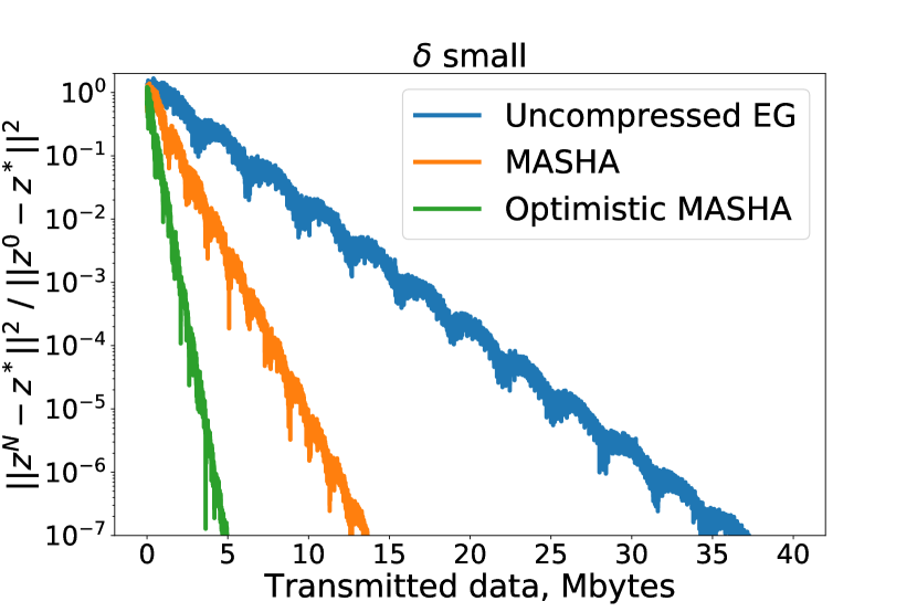
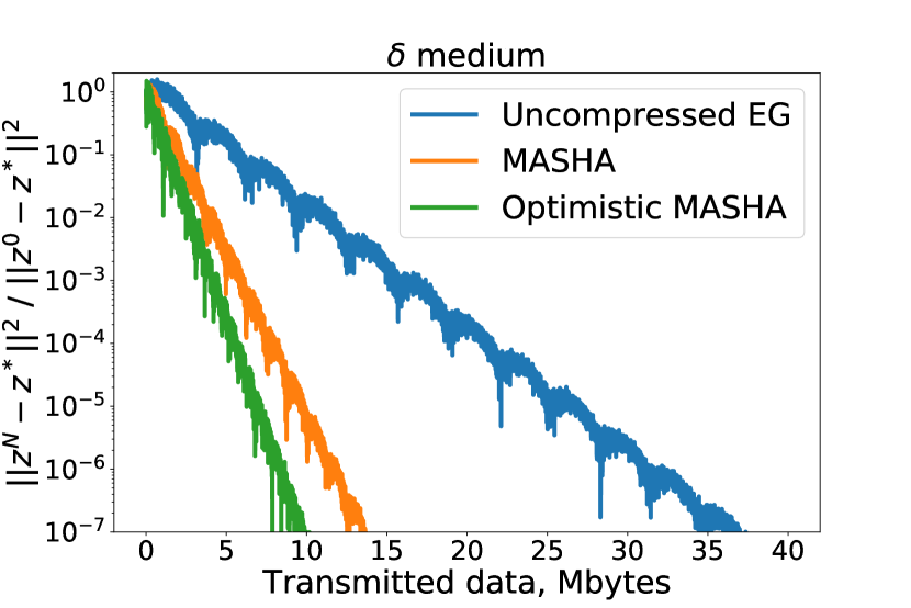
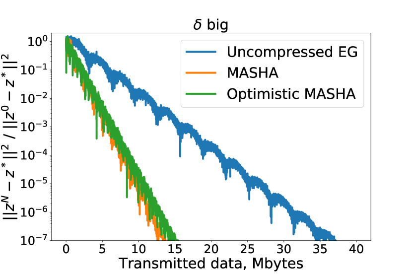
(a) small $\delta$

(b) medium $\delta$

(c) big $\delta$

Figure 1: Bilinear problem (9): Comparison of state-of-the-art methods with compression for variational inequalities for small, medium and big similarity parameters.

See Figure 1 for the results. For small $\delta$ Optimistic MASHA is about $\sqrt{M}$ times superior to MASHA, and also outperforms the uncompressed method by a factor of $M$. With increasing $\delta$ Optimistic MASHA comes close to MASHA in its convergence.

5 Conclusion

In this paper, we considered distributed methods for solving the variational inequality problem. We presented the new method Optimistic MASHA. By combining two techniques: compression and data similarity, our method allows us to significantly reduce the number of information transmitted during communications. Experiments confirm the theoretical conclusions.

Appendix 0.A Proof of Theorem 3.1

Lemma 2

Consider the problem (1) under Assumption 3. Let $\{z^{k}\}$ be the sequence generated by Algorithm 1 with compressors from Definition 1. Then, the following inequality holds:

$$\mathbb{E}\left[\left\|\Delta^{k}-\mathbb{E}_{k}\left[\Delta^{k}\right]\right\|^{2}\right]\leq 2\delta^{2}\mathbb{E}\left[\left\|z^{k}-w^{k-1}\right\|^{2}+\alpha^{2}\left\|z^{k}-z^{k-1}\right\|^{2}\right],$$ (10)

where $\mathbb{E}_{k}\left[\Delta^{k}\right]$ is equal to

$$\mathbb{E}_{k}\left[\Delta^{k}\right]=F(z^{k})+\alpha(F(z^{k})-F(z^{k-1})).$$ (11)

Proof

Due to the unbiasedness of $Q_{m}$, we can make sure that (11) is correct. Then using definitions of $\delta^{k}$ and $\Delta^{k}$ from Algorithm 1, we get

$$\mathbb{E}_{k}\left[\left\|\Delta^{k}-\mathbb{E}_{k}\left[\Delta^{k}\right]\right\|^{2}\right]$$

$$=\mathbb{E}_{k}\left[\left\|\frac{1}{M}\sum\limits_{m=1}^{M}Q_{m}(\delta^{k}_{m})+F(w^{k-1})-F(z^{k})-\alpha(F(z^{k})-F(z^{k-1}))\right\|^{2}\right]$$

$$=\mathbb{E}_{k}\left[\left\|\frac{1}{M}\sum\limits_{m=1}^{M}Q_{m}(\delta^{k}_{m})-\frac{1}{M}\sum\limits_{m=1}^{M}\delta^{k}_{m}\right\|^{2}\right].$$

By definition of $Q^{\text{dev}}_{m}$ (Lemma 1), we obtain

$$\mathbb{E}_{k}\left[\left\|\Delta^{k}-\mathbb{E}_{k}\left[\Delta^{k}\right]\right\|^{2}\right]$$

$$\leq\frac{1}{M}\sum\limits_{m=1}^{M}\left\|\delta^{k}_{m}-\frac{1}{M}\sum\limits_{m=1}^{M}\delta^{k}_{m}\right\|^{2}$$

$$=\frac{1}{M}\sum\limits_{m=1}^{M}\bigg{\|}F_{m}(z^{k})-F_{m}(w^{k-1})+\alpha[F_{m}(z^{k})-F_{m}(z^{k-1})]+F(w^{k-1})$$

$$\hskip 11.38092pt-F(z^{k})-\alpha(F(z^{k})-F(z^{k-1}))\bigg{\|}^{2}$$

$$=\frac{1}{M}\sum\limits_{m=1}^{M}\bigg{\|}F_{m}(z^{k})-F(z^{k})-F_{m}(w^{k-1})+F(w^{k-1})$$

$$\hskip 11.38092pt+\alpha[F_{m}(z^{k})-F(z^{k})-F_{m}(z^{k-1})+F(z^{k-1})]\bigg{\|}^{2}$$

$$\leq\frac{2}{M}\sum\limits_{m=1}^{M}\left\|F_{m}(z^{k})-F(z^{k})-F_{m}(w^{k-1})+F(w^{k-1})\right\|^{2}$$

$$\hskip 11.38092pt+\frac{2\alpha^{2}}{M}\sum\limits_{m=1}^{M}\left\|F_{m}(z^{k})-F(z^{k})-F_{m}(z^{k-1})+F(z^{k-1})\right\|^{2}.$$

Assumption on $\delta$-relatedness gives

$$\mathbb{E}_{k}\left[\left\|\Delta^{k}-\mathbb{E}_{k}\left[\Delta^{k}\right]\right\|^{2}\right]\leq 2\delta^{2}\left\|z^{k}-w^{k-1}\right\|^{2}+2\alpha^{2}\delta^{2}\left\|z^{k}-z^{k-1}\right\|^{2}.$$

This concludes the proof of (10).

$\square$

Before proving the main lemma of this section, we define the following Lyapunov function:

$$\Psi^{k+1} \vcentcolon=(1+2\mu\eta)\left\|z^{k+1}-z^{*}\right\|^{2}+\frac{\gamma+\eta\mu}{\gamma}\left\|w^{k+1}-z^{*}\right\|^{2}$$ (12)

$$\quad+2\eta\langle F(z^{k})-F(z^{k+1}),z^{k+1}-z^{*}\rangle+\gamma\left\|w^{k}-z^{k+1}\right\|^{2}+\frac{1}{8}\left\|z^{k+1}-z^{k}\right\|^{2}.$$

Lemma 3

Consider the problem (1) under Assumptions 1, 2 and 3. Let $\{z^{k}\}$ be the sequence generated by Algorithm 1 with compressors from Definition 1 and parameters

$$0<\gamma\leq\frac{1}{8},\quad\alpha\in(0;1),\quad\eta\leq\min\left\{\frac{\sqrt{\alpha\gamma}}{2\delta},\frac{1}{8(L+\delta)}\right\}.$$

Then, after $k$ iterations we get

$$\mathbb{E}\left[\frac{1}{2}\|z^{k}-z^{*}\|^{2}\right]\leq\max\left[\left(1-\frac{\mu\eta}{2}\right);\left(1-\frac{1}{\frac{1}{\eta\mu}+\frac{1}{\gamma}}\right);\alpha;\frac{1}{2}\right]\cdot^{k}\cdot\Psi^{0}.$$

Proof

We start from line 16 of Algorithm 1

$$\left\|z^{k+1}-z^{*}\right\|^{2}= \left\|z^{k}-z^{*}\right\|^{2}+2\langle z^{k+1}-z^{k},z^{k+1}-z^{*}\rangle-\left\|z^{k+1}-z^{k}\right\|^{2}$$

$$= \left\|z^{k}-z^{*}\right\|^{2}+2\gamma\langle w^{k}-z^{k},z^{k+1}-z^{*}\rangle$$

$$-2\eta\langle\Delta^{k}-F(z^{*}),z^{k+1}-z^{*}\rangle-\left\|z^{k+1}-z^{k}\right\|^{2}$$

$$-2\langle z^{k}+\gamma(w^{k}-z^{k})-\Delta^{k}-z^{k+1}+\eta F(z^{*}),z^{k+1}-z^{*}\rangle.$$

Optimality condition for (1) it follows, that

$$-F(z^{*})\in\partial g(z^{*}).$$

From update (line 16) for $z^{k+1}$ of Algorithm 1 it follows, that

$$z^{k}+\gamma(w^{k}-z^{k})-\eta\Delta^{k}-z^{k+1}\in\partial(\eta g)(z^{k+1}).$$

Hence, from monotonicity of $\partial g(\cdot)$ we get

$$\mathbb{E}\left[\left\|z^{k+1}-z^{*}\right\|^{2}\right] \leq\mathbb{E}\left[\left\|z^{k}-z^{*}\right\|^{2}\right]+2\gamma\mathbb{E}\left[\langle w^{k}-z^{k},z^{k+1}-z^{*}\rangle\right]$$

$$\quad-2\eta\mathbb{E}\left[\langle\Delta^{k}-F(z^{*}),z^{k+1}-z^{*}\rangle\right]-\mathbb{E}\left[\left\|z^{k+1}-z^{k}\right\|^{2}\right]$$

$$=\mathbb{E}\left[\left\|z^{k}-z^{*}\right\|^{2}\right]+2\gamma\mathbb{E}\left[\langle w^{k}-z^{*},z^{k+1}-z^{*}\rangle\right]$$

$$\quad-2\gamma\mathbb{E}\left[\langle z^{k}-z^{*},z^{k+1}-z^{*}\rangle\right]$$

$$\quad-2\eta\mathbb{E}\left[\langle\Delta^{k}-F(z^{*}),z^{k+1}-z^{*}\rangle\right]-\mathbb{E}\left[\left\|z^{k+1}-z^{k}\right\|^{2}\right]$$

$$=\mathbb{E}\left[\left\|z^{k}-z^{*}\right\|^{2}\right]$$

$$\quad+\gamma\mathbb{E}\left[\left\|w^{k}-z^{*}\right\|^{2}+\left\|z^{k+1}-z^{*}\right\|^{2}-\left\|z^{k+1}-w^{k}\right\|^{2}\right]$$

$$\quad-\gamma\mathbb{E}\left[\left\|z^{k+1}-z^{*}\right\|^{2}+\left\|z^{k}-z^{*}\right\|^{2}-\left\|z^{k+1}-z^{k}\right\|^{2}\right]$$

$$\quad-2\eta\mathbb{E}\left[\langle\Delta^{k}-F(z^{*}),z^{k+1}-z^{*}\rangle\right]-\mathbb{E}\left[\left\|z^{k+1}-z^{k}\right\|^{2}\right]$$

$$=\mathbb{E}\left[\left\|z^{k}-z^{*}\right\|^{2}\right]+\gamma\mathbb{E}\left[\left\|w^{k}-z^{*}\right\|^{2}\right]-\gamma\mathbb{E}\left[\left\|z^{k}-z^{*}\right\|^{2}\right]$$

$$\quad-\gamma\mathbb{E}\left[\left\|w^{k}-z^{k+1}\right\|^{2}\right]-2\eta\mathbb{E}\left[\langle\Delta^{k}-F(z^{*}),z^{k+1}-z^{*}\rangle\right]$$

$$\quad-(1-\gamma)\mathbb{E}\left[\left\|z^{k+1}-z^{k}\right\|^{2}\right].$$

In previous we also use the simple fact $\|a+b\|^{2}=\|a\|^{2}+2\langle a;b\rangle+\|b\|^{2}$ twice. Small rearrangement gives

$$\mathbb{E}\left[\left\|z^{k+1}-z^{*}\right\|^{2}\right] \leq\mathbb{E}\left[\left\|z^{k}-z^{*}\right\|^{2}\right]+\gamma\mathbb{E}\left[\left\|w^{k}-z^{*}\right\|^{2}\right]-\gamma\mathbb{E}\left[\left\|z^{k}-z^{*}\right\|^{2}\right]$$

$$\quad-\gamma\mathbb{E}\left[\left\|w^{k}-z^{k+1}\right\|^{2}\right]-(1-\gamma)\mathbb{E}\left[\left\|z^{k+1}-z^{k}\right\|^{2}\right]$$

$$\quad-2\eta\mathbb{E}\left[\langle\mathbb{E}_{k}\left[\Delta^{k}\right]-F(z^{*}),z^{k+1}-z^{*}\rangle\right]$$

$$\quad-2\eta\mathbb{E}\left[\langle\Delta^{k}-\mathbb{E}_{k}\left[\Delta^{k}\right],z^{k+1}-z^{k}\rangle\right]$$

$$\quad-2\eta\mathbb{E}\left[\langle\Delta^{k}-\mathbb{E}_{k}\left[\Delta^{k}\right],z^{k}-z^{*}\rangle\right].$$

Using the tower property of expectation we can obtain the following:

$$\mathbb{E}\left[\langle\mathbb{E}_{k}\left[\Delta^{k}\right]-\Delta^{k},z^{k}-z^{*}\rangle\right] =\mathbb{E}\left[\mathbb{E}_{k}\left[\langle\mathbb{E}_{k}\left[\Delta^{k}\right]-\Delta^{k},z^{k}-z^{*}\rangle\right]\right]$$

$$=\mathbb{E}\left[{\langle\mathbb{E}_{k}\left[\mathbb{E}_{k}\left[\Delta^{k}\right]-\Delta^{k}\right],z^{k}-z^{*}\rangle}\right]$$

$$=\mathbb{E}\left[{\langle\mathbb{E}_{k}\left[\Delta^{k}\right]-\mathbb{E}_{k}\left[\Delta^{k}\right],z^{k}-z^{*}\rangle}\right]=0.$$

Hence, with (11)

$$\mathbb{E}\left[\left\|z^{k+1}-z^{*}\right\|^{2}\right] \leq\mathbb{E}\left[\left\|z^{k}-z^{*}\right\|^{2}\right]+\gamma\mathbb{E}\left[\left\|z^{k}-z*\right\|^{2}\right]-\gamma\mathbb{E}\left[\left\|z^{k}-z^{*}\right\|^{2}\right]$$

$$\quad-\gamma\mathbb{E}\left[\left\|w^{k}-z^{k+1}\right\|^{2}\right]-(1-\gamma)\mathbb{E}\left[\left\|z^{k+1}-z^{k}\right\|^{2}\right]$$

$$\quad-2\eta\mathbb{E}\left[\langle F(z^{k})+\alpha(F(z^{k})-F(z^{k-1}))-F(z^{*}),z^{k+1}-z^{*}\rangle\right]$$

$$\quad+2\eta\mathbb{E}\left[\langle\mathbb{E}_{k}\left[\Delta^{k}\right]-\Delta^{k},z^{k+1}-z^{k}\rangle\right].$$

Using the Young’s inequality we get

$$\mathbb{E}\left[\left\|z^{k+1}-z^{*}\right\|^{2}\right] \leq\mathbb{E}\left[\left\|z^{k}-z^{*}\right\|^{2}\right]+\gamma\mathbb{E}\left[\left\|w^{k}-z^{*}\right\|^{2}\right]-\gamma\mathbb{E}\left[\left\|z^{k}-z^{*}\right\|^{2}\right]$$

$$\quad-\gamma\mathbb{E}\left[\left\|w^{k}-z^{k+1}\right\|^{2}\right]-(1-\gamma)\mathbb{E}\left[\left\|z^{k+1}-z^{k}\right\|^{2}\right]$$

$$\quad-2\eta\mathbb{E}\left[\langle F(z^{k})+\alpha(F(z^{k})-F(z^{k-1}))-F(z^{*}),z^{k+1}-z^{*}\rangle\right]$$

$$\quad+2\eta^{2}\mathbb{E}\left[\left\|\mathbb{E}_{k}\left[\Delta^{k}\right]-\Delta^{k}\right\|^{2}\right]+\frac{1}{2}\mathbb{E}\left[\left\|z^{k+1}-z^{k}\right\|^{2}\right]$$

$$=\mathbb{E}\left[\left\|z^{k}-z^{*}\right\|^{2}\right]+\gamma\mathbb{E}\left[\left\|w^{k}-z^{*}\right\|^{2}\right]-\gamma\mathbb{E}\left[\left\|z^{k}-z^{*}\right\|^{2}\right]$$

$$\quad-\gamma\mathbb{E}\left[\left\|w^{k}-z^{k+1}\right\|^{2}\right]-(1/2-\gamma)\mathbb{E}\left[\left\|z^{k+1}-z^{k}\right\|^{2}\right]$$

$$\quad+2\eta^{2}\mathbb{E}\left[\left\|\mathbb{E}_{k}\left[\Delta^{k}\right]-\Delta^{k}\right\|^{2}\right]$$

$$\quad-2\eta\mathbb{E}\left[\langle F(z^{k})+\alpha(F(z^{k})-F(z^{k-1}))-F(z^{*}),z^{k+1}-z^{*}\rangle\right].$$

By (10) we get

$$\mathbb{E}\left[\left\|z^{k+1}-z^{*}\right\|^{2}\right] \leq\mathbb{E}\left[\left\|z^{k}-z^{*}\right\|^{2}\right]+\gamma\mathbb{E}\left[\left\|w^{k}-z^{*}\right\|^{2}\right]-\gamma\mathbb{E}\left[\left\|z^{k}-z^{*}\right\|^{2}\right]$$

$$\quad-\gamma\mathbb{E}\left[\left\|w^{k}-z^{k+1}\right\|^{2}\right]-(1/2-\gamma)\mathbb{E}\left[\left\|z^{k+1}-z^{k}\right\|^{2}\right]$$

$$\quad+4\delta^{2}\eta^{2}\mathbb{E}\left[\left\|z^{k}-w^{k-1}\right\|^{2}\right]+4\alpha^{2}\delta^{2}\eta^{2}\mathbb{E}\left[\left\|z^{k}-z^{k-1}\right\|^{2}\right]$$

$$\quad-2\eta\mathbb{E}\left[\langle F(z^{k})+\alpha(F(z^{k})-F(z^{k-1}))-F(z^{*}),z^{k+1}-z^{*}\rangle\right]$$

$$=\mathbb{E}\left[\left\|z^{k}-z^{*}\right\|^{2}\right]-2\eta\mathbb{E}\left[\langle F(z^{k+1})-F(z^{*}),z^{k+1}-z^{*}\rangle\right]$$

$$\quad+\gamma\mathbb{E}\left[\left\|w^{k}-z^{*}\right\|^{2}\right]-\gamma\mathbb{E}\left[\left\|z^{k}-z^{*}\right\|^{2}\right]-\gamma\mathbb{E}\left[\left\|w^{k}-z^{k+1}\right\|^{2}\right]$$

$$\quad-(1/2-\gamma)\mathbb{E}\left[\left\|z^{k+1}-z^{k}\right\|^{2}\right]$$

$$\quad+4\delta^{2}\eta^{2}\mathbb{E}\left[\left\|z^{k}-w^{k-1}\right\|^{2}\right]+4\alpha^{2}\delta^{2}\eta^{2}\mathbb{E}\left[\left\|z^{k}-z^{k-1}\right\|^{2}\right]$$

$$\quad-2\eta\mathbb{E}\left[\langle F(z^{k})-F(z^{k+1})+\alpha(F(z^{k})-F(z^{k-1})),z^{k+1}-z^{*}\rangle\right].$$

Assumption 2 about $\mu$-strong monotonicity of $F$ gives

$$\mathbb{E}\left[\left\|z^{k+1}-z^{*}\right\|^{2}\right]$$

$$\leq\mathbb{E}\left[\left\|z^{k}-z^{*}\right\|^{2}\right]-2\mu\eta\mathbb{E}\left[\left\|z^{k+1}-z^{*}\right\|^{2}\right]+\gamma\mathbb{E}\left[\left\|w^{k}-z^{*}\right\|^{2}\right]-\gamma\mathbb{E}\left[\left\|z^{k}-z^{*}\right\|^{2}\right]$$

$$\quad-\gamma\mathbb{E}\left[\left\|w^{k}-z^{k+1}\right\|^{2}\right]-(1/2-\gamma)\mathbb{E}\left[\left\|z^{k+1}-z^{k}\right\|^{2}\right]$$

$$\quad+4\delta^{2}\eta^{2}\mathbb{E}\left[\left\|z^{k}-w^{k-1}\right\|^{2}\right]+4\alpha^{2}\delta^{2}\eta^{2}\mathbb{E}\left[\left\|z^{k}-z^{k-1}\right\|^{2}\right]$$

$$\quad-2\eta\mathbb{E}\left[\langle F(z^{k})-F(z^{k+1})+\alpha(F(z^{k})-F(z^{k-1})),z^{k+1}-z^{*}\rangle\right]$$

$$=\mathbb{E}\left[\left\|z^{k}-z^{*}\right\|^{2}\right]-2\mu\eta\mathbb{E}\left[\left\|z^{k+1}-z^{*}\right\|^{2}\right]+\gamma\mathbb{E}\left[\left\|w^{k}-z^{*}\right\|^{2}\right]-\gamma\mathbb{E}\left[\left\|z^{k}-z^{*}\right\|^{2}\right]$$

$$\quad-\gamma\mathbb{E}\left[\left\|w^{k}-z^{k+1}\right\|^{2}\right]-(1/2-\gamma)\mathbb{E}\left[\left\|z^{k+1}-z^{k}\right\|^{2}\right]$$

$$\quad+4\delta^{2}\eta^{2}\mathbb{E}\left[\left\|z^{k}-w^{k-1}\right\|^{2}\right]+4\alpha^{2}\delta^{2}\eta^{2}\mathbb{E}\left[\left\|z^{k}-z^{k-1}\right\|^{2}\right]$$

$$\quad-2\eta\mathbb{E}\left[\langle F(z^{k})-F(z^{k+1}),z^{k+1}-z^{*}\rangle\right]$$

$$\quad-2\alpha\eta\mathbb{E}\left[\langle F(z^{k})-F(z^{k-1}),z^{k}-z^{*}\rangle\right]$$

$$\quad-2\alpha\eta\mathbb{E}\left[\langle F(z^{k})-F(z^{k-1}),z^{k+1}-z^{k}\rangle\right].$$

With small rearrangement and Young’s inequality we get

$$\mathbb{E}\left[\left\|z^{k+1}-z^{*}\right\|^{2}\right]+2\eta\mathbb{E}\left[\langle F(z^{k})-F(z^{k+1}),z^{k+1}-z^{*}\rangle\right]$$

$$\leq\mathbb{E}\left[\left\|z^{k}-z^{*}\right\|^{2}\right]-2\mu\eta\mathbb{E}\left[\left\|z^{k+1}-z^{*}\right\|^{2}\right]+\gamma\mathbb{E}\left[\left\|w^{k}-z^{*}\right\|^{2}\right]$$

$$\quad-\gamma\mathbb{E}\left[\left\|z^{k}-z^{*}\right\|^{2}\right]+\alpha\cdot 2\eta\mathbb{E}\left[\langle F(z^{k-1})-F(z^{k}),z^{k}-z^{*}\rangle\right]$$

$$\quad-\gamma\mathbb{E}\left[\left\|w^{k}-z^{k+1}\right\|^{2}\right]-(1/2-\gamma)\mathbb{E}\left[\left\|z^{k+1}-z^{k}\right\|^{2}\right]$$

$$\quad+4\delta^{2}\eta^{2}\mathbb{E}\left[\left\|z^{k}-w^{k-1}\right\|^{2}\right]+4\alpha^{2}\delta^{2}\eta^{2}\mathbb{E}\left[\left\|z^{k}-z^{k-1}\right\|^{2}\right]$$

$$\quad+4\alpha^{2}\eta^{2}\mathbb{E}\left[\left\|F(z^{k})-F(z^{k-1})\right\|^{2}\right]+\frac{1}{4}\mathbb{E}\left[\left\|z^{k+1}-z^{k}\right\|^{2}\right].$$

With $L$-Lipshitzness of $F$ (Assumption 1) and $\gamma\leq\frac{1}{8}$, we have

$$\mathbb{E}\left[\left\|z^{k+1}-z^{*}\right\|^{2}\right]+2\eta\mathbb{E}\left[\langle F(z^{k})-F(z^{k+1}),z^{k+1}-z^{*}\rangle\right]$$

$$\leq\mathbb{E}\left[\left\|z^{k}-z^{*}\right\|^{2}\right]-2\mu\eta\mathbb{E}\left[\left\|z^{k+1}-z^{*}\right\|^{2}\right]+\gamma\mathbb{E}\left[\left\|w^{k}-z^{*}\right\|^{2}\right]$$

$$\quad-\gamma\mathbb{E}\left[\left\|z^{k}-z^{*}\right\|^{2}\right]+\alpha\cdot 2\eta\mathbb{E}\left[\langle F(z^{k-1})-F(z^{k}),z^{k}-z^{*}\rangle\right]$$

$$\quad-\gamma\mathbb{E}\left[\left\|w^{k}-z^{k+1}\right\|^{2}\right]+4\delta^{2}\eta^{2}\mathbb{E}\left[\left\|z^{k}-w^{k-1}\right\|^{2}\right]-\frac{1}{8}\mathbb{E}\left[\left\|z^{k+1}-z^{k}\right\|^{2}\right]$$

$$\quad+4\alpha^{2}\delta^{2}\eta^{2}\mathbb{E}\left[\left\|z^{k}-z^{k-1}\right\|^{2}\right]+4\alpha^{2}L^{2}\eta^{2}\mathbb{E}\left[\left\|z^{k}-z^{k-1}\right\|^{2}\right].$$

Now, we add $\tfrac{\gamma+\eta\mu}{\gamma}\mathbb{E}\left[\left\|w^{k+1}-z^{*}\right\|^{2}\right]$ to both sides and use update for $w^{k+1}$ (lines 18 and 22 of Algorithm 1)

$$\frac{\gamma+\eta\mu}{\gamma}\mathbb{E}\left[\mathbb{E}_{w^{k+1}}{\left\|w^{k+1}-z^{*}\right\|^{2}}\right] =(\gamma+\eta\mu)\mathbb{E}\left[\left\|z^{k}-z^{*}\right\|^{2}\right]$$

$$\quad+\frac{(\gamma+\eta\mu)(1-\gamma)}{\gamma}\mathbb{E}\left[\left\|w^{k}-z^{*}\right\|^{2}\right],$$

and get

$$(1+2\mu\eta) \mathbb{E}\left[\left\|z^{k+1}-z^{*}\right\|^{2}\right]+\frac{\gamma+\eta\mu}{\gamma}\mathbb{E}\left[\left\|w^{k+1}-z^{*}\right\|^{2}\right]$$

$$\quad+2\eta\mathbb{E}\left[\langle F(z^{k})-F(z^{k+1}),z^{k+1}-z^{*}\rangle\right]$$

$$\quad+\gamma\mathbb{E}\left[\left\|w^{k}-z^{k+1}\right\|^{2}\right]+\frac{1}{8}\mathbb{E}\left[\left\|z^{k+1}-z^{k}\right\|^{2}\right]$$

$$\leq(1+\eta\mu)\mathbb{E}\left[\left\|z^{k}-z^{*}\right\|^{2}\right]+\gamma\mathbb{E}\left[\left\|w^{k}-z^{*}\right\|^{2}\right]$$

$$\quad+\frac{(\gamma+\eta\mu)(1-\gamma)}{\gamma}\mathbb{E}\left[\left\|w^{k}-z^{*}\right\|^{2}\right]$$

$$\quad+\alpha\cdot 2\eta\mathbb{E}\left[\langle F(z^{k-1})-F(z^{k}),z^{k}-z^{*}\rangle\right]$$

$$\quad+\frac{4\delta^{2}\eta^{2}}{\gamma}\cdot\gamma\mathbb{E}\left[\left\|w^{k-1}-z^{k}\right\|^{2}\right]$$

$$\quad+32\alpha^{2}(\delta^{2}+L^{2})\eta^{2}\cdot\frac{1}{8}\mathbb{E}\left[\left\|z^{k}-z^{k-1}\right\|^{2}\right].$$

Note that $\eta\leq\min\left\{\frac{\sqrt{\alpha\gamma}}{2\delta},\frac{1}{8(L+\delta)}\right\}$, $0<\alpha<1$, $0<\gamma<1$ and $L\geq\mu$, then we get that

$$\frac{4\delta^{2}\eta^{2}}{\gamma}\leq\alpha;\quad 32\alpha^{2}(\delta^{2}+L^{2})\eta^{2}\leq\frac{1}{2};\quad(1+\mu\eta)\leq\left(1-\frac{\mu\eta}{2}\right)(1+2\mu\eta);$$

$$\gamma+\frac{(\gamma+\eta\mu)(1-\gamma)}{\gamma}=\left(1-\frac{1}{\frac{1}{\eta\mu}+\frac{1}{\gamma}}\right)\frac{\gamma+\eta\mu}{\gamma}$$

Hence, it holds

$$(1+2\mu\eta) \mathbb{E}\left[\left\|z^{k+1}-z^{*}\right\|^{2}\right]+\frac{\gamma+\eta\mu}{\gamma}\mathbb{E}\left[\left\|w^{k+1}-z^{*}\right\|^{2}\right]$$

$$\quad+2\eta\mathbb{E}\left[\langle F(z^{k})-F(z^{k+1}),z^{k+1}-z^{*}\rangle\right]$$

$$\quad+\gamma\mathbb{E}\left[\left\|w^{k}-z^{k+1}\right\|^{2}\right]+\frac{1}{8}\mathbb{E}\left[\left\|z^{k+1}-z^{k}\right\|^{2}\right]$$

$$\leq\left(1-\frac{\mu\eta}{2}\right)\cdot(1+2\eta\mu)\mathbb{E}\left[\left\|z^{k}-z^{*}\right\|^{2}\right]$$

$$\quad+\left(1-\frac{1}{\frac{1}{\eta\mu}+\frac{1}{\gamma}}\right)\cdot\frac{\gamma+\eta\mu}{\gamma}\mathbb{E}\left[\left\|w^{k}-z^{*}\right\|^{2}\right]$$

$$\quad+\alpha\cdot 2\eta\mathbb{E}\left[\langle F(z^{k-1})-F(z^{k}),z^{k}-z^{*}\rangle\right]$$

$$\quad+\alpha\cdot\gamma\mathbb{E}\left[\left\|w^{k-1}-z^{k}\right\|^{2}\right]$$

$$\quad+\frac{1}{2}\cdot\frac{1}{8}\mathbb{E}\left[\left\|z^{k}-z^{k-1}\right\|^{2}\right].$$

Definition (12) of the Lyapunov function move us to

$$\mathbb{E}\left[\Psi^{k+1}\right]\leq\max\left[\left(1-\frac{\mu\eta}{2}\right);\left(1-\frac{1}{\frac{1}{\eta\mu}+\frac{1}{\gamma}}\right);\alpha;\frac{1}{2}\right]\cdot\mathbb{E}\left[\Psi^{k}\right].$$

It remains to show, that

$$\Psi^{k}\geq\frac{1}{2}\left\|z^{k}-z^{*}\right\|^{2}.$$

$$\Psi^{k} \geq\left\|z^{k}-z^{*}\right\|^{2}+\frac{1}{8}\left\|z^{k}-z^{k-1}\right\|^{2}+2\eta\langle F(z^{k})-F(z^{k-1}),z^{*}-z^{k}\rangle$$

$$\geq\left\|z^{k}-z^{*}\right\|^{2}+\frac{1}{8}\left\|z^{k}-z^{k-1}\right\|^{2}-\frac{1}{2}\left\|z^{k}-z^{*}\right\|^{2}-2\eta^{2}\left\|F(z^{k})-F(z^{k-1})\right\|^{2}.$$

Using $L$-Lipschitzness of $F$ we get

$$\Psi^{k} \geq\frac{1}{2}\left\|z^{k}-z^{*}\right\|^{2}+\frac{1}{8}\left(1-16L^{2}\eta^{2}\right)\left\|z^{k}-z^{k-1}\right\|^{2}.$$

With $\eta\leq\frac{1}{8L}$, we get

$$\Psi^{k}\geq\frac{1}{2}\left\|z^{k}-z^{*}\right\|^{2}.$$

Theorem 0.A.1 (Theorem 3.1)

Consider the problem (1) under Assumptions 1, 2 and 3. Let $\{z^{k}\}$ be the sequence generated by Algorithm 1 with compressors from Definition 1 and parameters

$$0<\gamma\leq\frac{1}{8},\quad\alpha=\frac{1}{2},\quad\eta=\min\left\{\frac{\sqrt{\alpha\gamma}}{2\delta},\frac{1}{8(L+\delta)}\right\}.$$

Then, given $\varepsilon>0$, the number of iterations for $\|z^{k}-z^{*}\|^{2}\leq\varepsilon$ is

$$O\left(\left[\frac{1}{\gamma}+\frac{L}{\mu}+\frac{\delta}{\sqrt{\gamma}\mu}\right]\log\frac{1}{\varepsilon}\right).$$

Proof

From Lemma 3 we can get that the iteration complexity of Algorithm 1:

$$O\left(\left[1+\frac{1}{\eta\mu}+\frac{1}{\gamma}\right]\log\frac{1}{\varepsilon}\right) =O\left(\left[\frac{1}{\gamma}+\frac{\delta}{\mu}+\frac{L}{\mu}+\frac{\delta}{\sqrt{\gamma}\mu}\right]\log\frac{1}{\varepsilon}\right)$$

$$=O\left(\left[\frac{1}{\gamma}+\frac{L}{\mu}+\frac{\delta}{\sqrt{\gamma}\mu}\right]\log\frac{1}{\varepsilon}\right).$$

References

- [1] Agafonov, A., Dvurechensky, P., Scutari, G., Gasnikov, A., Kamzolov, D., Lukashevich, A., Daneshmand, A.: An accelerated second-order method for distributed stochastic optimization. arXiv preprint arXiv:2103.14392 (2021)
- [2] Alacaoglu, A., Malitsky, Y.: Stochastic variance reduction for variational inequality methods. arXiv preprint arXiv:2102.08352 (2021)
- [3] Alistarh, D., Grubic, D., Li, J., Tomioka, R., Vojnovic, M.: QSGD: Communication-efficient SGD via gradient quantization and encoding. In: Advances in Neural Information Processing Systems. pp. 1709–1720 (2017)
- [4] Arjevani, Y., Shamir, O.: Communication complexity of distributed convex learning and optimization. Advances in neural information processing systems 28 (2015)
- [5] Bach, F., Jenatton, R., Mairal, J., Obozinski, G.: Optimization with sparsity-inducing penalties. arXiv preprint arXiv:1108.0775 (2011)
- [6] Bach, F., Mairal, J., Ponce, J.: Convex sparse matrix factorizations. arXiv preprint arXiv:0812.1869 (2008)
- [7] Bauschke, H., Combettes, P.: Convex Analysis and Monotone Operator Theory in Hilbert Spaces (01 2017). https://doi.org/10.1007/978-3-319-48311-5
- [8] Ben-Tal, A., Ghaoui, L.E., Nemirovski, A.: Robust Optimization. Princeton University Press (2009)
- [9] Beznosikov, A., Horváth, S., Richtárik, P., Safaryan, M.: On biased compression for distributed learning. arXiv preprint arXiv:2002.12410 (2020)
- [10] Beznosikov, A., Richtárik, P., Diskin, M., Ryabinin, M., Gasnikov, A.: Distributed methods with compressed communication for solving variational inequalities, with theoretical guarantees. arXiv preprint arXiv:2110.03313 (2021)
- [11] Beznosikov, A., Samokhin, V., Gasnikov, A.: Local sgd for saddle-point problems. arXiv preprint arXiv:2010.13112 (2020)
- [12] Beznosikov, A., Scutari, G., Rogozin, A., Gasnikov, A.: Distributed saddle-point problems under data similarity. Advances in Neural Information Processing Systems 34 (2021)
- [13] Chambolle, A., Pock, T.: A first-order primal-dual algorithm for convex problems with applications to imaging. Journal of mathematical imaging and vision 40(1), 120–145 (2011)
- [14] Chavdarova, T., Gidel, G., Fleuret, F., Lacoste-Julien, S.: Reducing noise in gan training with variance reduced extragradient. arXiv preprint arXiv:1904.08598 (2019)
- [15] Daneshmand, A., Scutari, G., Dvurechensky, P., Gasnikov, A.: Newton method over networks is fast up to the statistical precision. In: International Conference on Machine Learning. pp. 2398–2409. PMLR (2021)
- [16] Daskalakis, C., Ilyas, A., Syrgkanis, V., Zeng, H.: Training gans with optimism. arXiv preprint arXiv:1711.00141 (2017)
- [17] Esser, E., Zhang, X., Chan, T.F.: A general framework for a class of first order primal-dual algorithms for convex optimization in imaging science. SIAM Journal on Imaging Sciences 3(4), 1015–1046 (2010)
- [18] Facchinei, F., Pang, J.: Finite-Dimensional Variational Inequalities and Complementarity Problems. Springer Series in Operations Research and Financial Engineering, Springer New York (2007), https://books.google.ru/books?id=lX_7Rce3_Q0C
- [19] Facchinei, F., Pang, J.S.: Finite-Dimensional Variational Inequalities and Complementarity Problems. Springer Series in Operations Research, Springer (2003)
- [20] Ghosh, A., Maity, R.K., Mazumdar, A., Ramchandran, K.: Communication efficient distributed approximate Newton method. In: IEEE International Symposium on Information Theory (ISIT) (2020). https://doi.org/10.1109/ISIT44484.2020.9174216
- [21] Gidel, G., Berard, H., Vignoud, G., Vincent, P., Lacoste-Julien, S.: A variational inequality perspective on generative adversarial networks. arXiv preprint arXiv:1802.10551 (2018)
- [22] Goodfellow, I.J., Pouget-Abadie, J., Mirza, M., Xu, B., Warde-Farley, D., Ozair, S., Courville, A., Bengio, Y.: Generative adversarial networks (2014)
- [23] Gorbunov, E., Burlachenko, K., Li, Z., Richtárik, P.: MARINA: Faster non-convex distributed learning with compression. In: 38th International Conference on Machine Learning (2021)
- [24] Hendrikx, H., Xiao, L., Bubeck, S., Bach, F., Massoulie, L.: Statistically preconditioned accelerated gradient method for distributed optimization. In: International Conference on Machine Learning. pp. 4203–4227. PMLR (2020)
- [25] Horváth, S., Kovalev, D., Mishchenko, K., Stich, S., Richtárik, P.: Stochastic distributed learning with gradient quantization and variance reduction. arXiv preprint arXiv:1904.05115 (2019)
- [26] Horváth, S., Richtárik, P.: A better alternative to error feedback for communication-efficient distributed learning. arXiv preprint arXiv:2006.11077 (2020)
- [27] Juditsky, A., Nemirovskii, A.S., Tauvel, C.: Solving variational inequalities with stochastic mirror-prox algorithm (2008)
- [28] Karimireddy, S.P., Rebjock, Q., Stich, S., Jaggi, M.: Error feedback fixes signsgd and other gradient compression schemes. In: International Conference on Machine Learning. pp. 3252–3261. PMLR (2019)
- [29] Konečný, J., McMahan, H.B., Yu, F., Richtárik, P., Suresh, A.T., Bacon, D.: Federated learning: strategies for improving communication efficiency. In: NIPS Private Multi-Party Machine Learning Workshop (2016)
- [30] Korpelevich, G.M.: The extragradient method for finding saddle points and other problems (1976)
- [31] Kovalev, D., Beznosikov, A., Borodich, E., Gasnikov, A., Scutari, G.: Optimal gradient sliding and its application to distributed optimization under similarity. arXiv preprint arXiv:2205.15136 (2022)
- [32] Kovalev, D., Beznosikov, A., Sadiev, A., Persiianov, M., Richtárik, P., Gasnikov, A.: Optimal algorithms for decentralized stochastic variational inequalities. arXiv preprint arXiv:2202.02771 (2022)
- [33] Li, Z., Kovalev, D., Qian, X., Richtárik, P.: Acceleration for compressed gradient descent in distributed and federated optimization. arXiv preprint arXiv:2002.11364 (2020)
- [34] Liang, T., Stokes, J.: Interaction matters: A note on non-asymptotic local convergence of generative adversarial networks. In: Chaudhuri, K., Sugiyama, M. (eds.) Proceedings of the Twenty-Second International Conference on Artificial Intelligence and Statistics. Proceedings of Machine Learning Research, vol. 89, pp. 907–915. PMLR (16–18 Apr 2019), https://proceedings.mlr.press/v89/liang19b.html
- [35] Mertikopoulos, P., Lecouat, B., Zenati, H., Foo, C.S., Chandrasekhar, V., Piliouras, G.: Optimistic mirror descent in saddle-point problems: Going the extra (gradient) mile. arXiv preprint arXiv:1807.02629 (2018)
- [36] Mishchenko, K., Gorbunov, E., Takáč, M., Richtárik, P.: Distributed learning with compressed gradient differences. arXiv preprint arXiv:1901.09269 (2019)
- [37] Nemirovski, A.: Prox-method with rate of convergence o (1/t) for variational inequalities with lipschitz continuous monotone operators and smooth convex-concave saddle point problems. SIAM Journal on Optimization 15(1), 229–251 (2004)
- [38] Nemirovski, A.: Prox-method with rate of convergence o(1/t) for variational inequalities with lipschitz continuous monotone operators and smooth convex-concave saddle point problems. SIAM Journal on Optimization 15, 229–251 (01 2004). https://doi.org/10.1137/S1052623403425629
- [39] Nesterov, Y.: Smooth minimization of non-smooth functions. Mathematical programming 103(1), 127–152 (2005)
- [40] Peng, W., Dai, Y.H., Zhang, H., Cheng, L.: Training gans with centripetal acceleration. Optimization Methods and Software 35(5), 955–973 (2020)
- [41] Philippenko, C., Dieuleveut, A.: Bidirectional compression in heterogeneous settings for distributed or federated learning with partial participation: tight convergence guarantees. arXiv preprint arXiv:2006.14591 (2020)
- [42] Reddi, S.J., Konečnỳ, J., Richtárik, P., Póczós, B., Smola, A.: Aide: Fast and communication efficient distributed optimization. arXiv preprint arXiv:1608.06879 (2016)
- [43] Richtárik, P., Sokolov, I., Fatkhullin, I.: EF21: A new, simpler, theoretically better, and practically faster error feedback. arXiv preprint arXiv:2106.05203 (2021)
- [44] Shamir, O., Srebro, N., Zhang, T.: Communication-efficient distributed optimization using an approximate newton-type method. In: Xing, E.P., Jebara, T. (eds.) Proceedings of the 31st International Conference on Machine Learning. Proceedings of Machine Learning Research, vol. 32, pp. 1000–1008. PMLR, Bejing, China (22–24 Jun 2014), https://proceedings.mlr.press/v32/shamir14.html
- [45] Smith, V., Forte, S., Ma, C., Takáč, M., Jordan, M.I., Jaggi, M.: CoCoA: A general framework for communication-efficient distributed optimization. Journal of Machine Learning Research 18, 1–49 (2018)
- [46] Szlendak, R., Tyurin, A., Richtárik, P.: Permutation compressors for provably faster distributed nonconvex optimization. arXiv preprint arXiv:2110.03300 (2021)
- [47] Tang, H., Yu, C., Lian, X., Zhang, T., Liu, J.: Doublesqueeze: Parallel stochastic gradient descent with double-pass error-compensated compression. In: International Conference on Machine Learning. pp. 6155–6165. PMLR (2019)
- [48] Tian, Y., Scutari, G., Cao, T., Gasnikov, A.: Acceleration in distributed optimization under similarity. arXiv preprint arXiv:2110.12347 (2021)
- [49] Tropp, J.A.: An introduction to matrix concentration inequalities. arXiv preprint arXiv:1501.01571 (2015)
- [50] Verbraeken, J., Wolting, M., Katzy, J., Kloppenburg, J., Verbelen, T., Rellermeyer, J.S.: A survey on distributed machine learning. ACM Computing Surveys (2019)
- [51] Yuan, X.T., Li, P.: On convergence of distributed approximate newton methods: Globalization, sharper bounds and beyond. arXiv preprint arXiv:1908.02246 (2019)
- [52] Zhang, Y., Lin, X.: Disco: Distributed optimization for self-concordant empirical loss. In: Bach, F., Blei, D. (eds.) Proceedings of the 32nd International Conference on Machine Learning. Proceedings of Machine Learning Research, vol. 37, pp. 362–370. PMLR, Lille, France (07–09 Jul 2015), https://proceedings.mlr.press/v37/zhangb15.html
- [53] Zheng, S., Huang, Z., Kwok, J.: Communication-efficient distributed blockwise momentum sgd with error-feedback. Advances in Neural Information Processing Systems 32, 11450–11460 (2019)