Bayesian non-conjugate regression
via variational message passing

Abstract

Variational inference is a popular method for approximating the posterior distribution of hierarchical Bayesian models. It is well-recognized in the literature that the choice of the approximation family and the regularity properties of the posterior strongly influence the efficiency and accuracy of variational methods. While model-specific conjugate approximations offer simplicity, they often converge slowly and may yield poor approximations. Non-conjugate approximations instead are more flexible but typically require the calculation of expensive multidimensional integrals. This study focuses on Bayesian regression models that use possibly non-differentiable loss functions to measure prediction misfit. The data behavior is modeled using a linear predictor, potentially transformed using a bijective link function. Examples include generalized linear models, mixed additive models, support vector machines, and quantile regression. To address the limitations of non-conjugate settings, the study proposes an efficient non-conjugate variational message passing method for approximate posterior inference, which only requires the calculation of univariate numerical integrals when analytical solutions are not available. The approach does not require differentiability, conjugacy, or model-specific data-augmentation strategies, thereby naturally extending to models with non-conjugate likelihood functions. Additionally, a stochastic implementation is provided to handle large-scale data problems. The proposed method’s performances are evaluated through extensive simulations and real data examples. Overall, the results highlight the effectiveness of the proposed variational message passing method, demonstrating its computational efficiency and approximation accuracy as an alternative to existing methods in Bayesian inference for regression models.

Keywords: General Bayesian inference; Mixed regression models; Non-conjugate models; Variational message passing.

1 Introduction

The increasing prevalence of big volume and velocity data, eventually coming from different data sources, entails a great opportunity but also a major challenge of modern data analysis and, in particular, of Bayesian statistics. The computational burden required by Markov chain Monte Carlo simulation (Gelman et al.,, 2013), that is the state-of-the-art approach to Bayesian inference, is often not compatible with time constraints and memory limits. Therefore, in the last two decades many efforts have been spent to develop alternative estimation methods not involving posterior simulation. In this context, optimization-based algorithms play an important role because of their ability to provide a reasonably good approximation of the posterior, while keeping a high level of efficiency. Within this family, two important examples are the Laplace approximation (Raftery,, 1996), along with its integrated nested generalization (Rue et al.,, 2009), and the variational inference approach, which includes, among others, local variational approximation (Jaakkola and Jordan,, 2000), mean field variational Bayes (Ormerod and Wand,, 2010; Blei et al.,, 2017), expectation propagation (Minka,, 2013; Bishop,, 2006, Chapter 10), stochastic variational inference (Hoffman et al.,, 2013), black-box variational inference (Ranganath et al.,, 2014; Kucukelbir et al.,, 2017; Ong et al.,, 2018) and natural gradient variational inference (Khan and Lin,, 2017; Khan and Nielsen,, 2018). All of these are mainly concerned with the estimation of hierarchical Bayesian models with a regular likelihood function, often belonging to the exponential family. For instance, both Laplace approximation and stochastic variational inference require for the log-likelihood function to be differentiable with continuity from one to three times, depending on the implementation. On the other hand, mean field variational Bayes and expectation propagation are employed when the hierarchical model can be described through a Bayesian factor graph with locally conjugate nodes, like for the Gibbs sampling algorithm (Gelman et al.,, 2013).

The joint lack of smoothness and conjugacy constitutes one of the main issues when it comes to approximating a posterior density. In such cases, well-designed data-augmentation strategies might help in representing an elaborate distribution (Wand et al.,, 2011) as the marginal law of an enlarged joint model by introducing a set of latent working variables. This tool, firstly introduced for motivating the expectation-maximization algorithm (Dempster et al.,, 1977), usually permits to restore the regularity in the augmented parameter space, drastically simplifying the calculations. Though, a convenient stochastic representation is not always available and sometimes can lead to important computational drawbacks, mainly concerned with a slowdown of the convergence speed and a worsening of the approximation quality in the original parameter space. See, for instance, Lewandowski et al., (2010), Neville et al., (2014), Duan et al., (2018) and Johndrow et al., (2019) for an up-to-date discussion on this topic. Furthermore, the lack of general recipes for extending model-specific augmentation techniques strongly narrows the range of applications of such an approach for solving general inferential problems. A classical example is given by Binomial regression models, for which data-augmented representations are available only under probit and logit links, while they are not for, e.g., Cauchy and complementary log-log links.

Many of these issues are amplified when the parameters of interest do not index a known family of probability distributions but are defined according to a minimum risk criterion and are linked to the data through a loss function. In these cases, the minimal regularity conditions for an estimation problem to be well-defined may not be satisfied, as it happens for support vector machines (Vapnik,, 1998), quantile and expectile regression (Koenker,, 2005).

The present work aims to introduce a unified, yet simple to implement, variational methodology for approximating the general posterior distribution of Bayesian mixed regression models (Bissiri et al.,, 2016). Specifically, we here consider regression and classification models predicting the response variable through a linear predictor, eventually transformed using a bijective link, and where the prediction misfit is measured by either a loss function or a pseudo-likelihood. Such a formulation includes as special cases generalized linear models and generalized estimating equations (see, e.g., McCullagh and Nelder,, 1989). We deserve particular attention to loss functions characterized by non-regular, i.e. non-differentiable and non-conjugate, behavior and for which standard Bayesian approximation techniques can not be directly employed or may suffer severe drawbacks, such as slow convergence or poor approximation quality.

Starting from a general formulation of non-conjugate variational message passing (Knowles and Minka,, 2011; Wand,, 2014; Rohde and Wand,, 2016), we develop both deterministic and stochastic optimization algorithms to perform variational inference for linear mixed models. Doing this, we obtain numerical methods which mimic, in their formulation, the penalized reweighted least squares algorithm for generalized linear models (McCullagh and Nelder,, 1989), where the derivatives of the likelihood with respect to the linear predictor are replaced by their variational expectations. This formulation has two main advantages: it only involves the calculation of univariate integrals, instead of multidimensional ones, and, in addition, it easily applies to non-differentiable losses. Indeed, the variational expectation of the loss derivatives is well-defined and easy to compute even when the proper loss derivatives are not. Moreover, the proposed method theoretically outperforms, in Kullback-Leibler divergence, the state-of-the-art mean field variational Bayes approximations based on conjugate data-augmented representations while maintaining the same level of computational efficiency.

In this framework, an additional benefit of the proposed approach is to combine the efficiency and modularity of mean field variational Bayes (Ormerod and Wand,, 2010; Blei et al.,, 2017) with the flexibility of Gaussian variational approximations (Wand,, 2014) to deal with parameters not having a conjugate distribution. Previously similar strategies, such as semiparametric variational Bayes (Rohde and Wand,, 2016), or natural gradient approach (Khan and Lin,, 2017; Khan and Nielsen,, 2018), has been used for the estimation of Bayesian generalized linear mixed models (Ormerod and Wand,, 2012; Tan and Nott,, 2013), semiparametric models for overdispersed count data (Luts and Wand,, 2015), semiparametric heteroscedastic regression (Menictas and Wand,, 2015) and Gaussian process regression (Opper and Archambeau,, 2009; Khan and Lin,, 2017).

The article is organized as follows. Section 2 reviews some fundamental concepts of mean field variational inference and non-conjugate variational message passing. Section 3 describes the proposed message passing methods for linear mixed models, characterizes their properties and presents several examples for both regular and non-regular models, including quantile regression and support vector machines. Section 4 provide a theoretical connection between our approach and augmented-data mean field variational Bayes. Section 5 presents an extensive simulation study designed to evaluate the quality and the efficiency the proposed approximation with respect to gold standard methods in the literature. Section 6 discuss four real-data examples concerned with electric power consumption in US, air quality measurements in Beijing, a bank marketing study in Portugal and a forest cover-type analysis in Colorado. Section 7 is devoted to a closing discussion.

2 Variational learning

Let $\pi(\mathbf{y}|\boldsymbol{\theta})$ be a generic statistical model for the observed data vector $\mathbf{y}=(y_{1},\dots,y_{n})^{\top}$ and the unknown parameter vector $\boldsymbol{\theta}\in\Theta$, which has prior distribution $\pi(\boldsymbol{\theta})$. We here consider either proper generative models, where $\pi(\mathbf{y}|\boldsymbol{\theta})\propto\exp\{\ell(\boldsymbol{\theta};\mathbf{y})\}$ is a genuine likelihood function, and risk based models, where $\pi(\mathbf{y}|\boldsymbol{\theta})\propto\exp\{-nR_{n}(\boldsymbol{\theta})/\phi\}$ denotes a pseudo-likelihood function with empirical risk $R_{n}(\boldsymbol{\theta})=\sum_{i=1}^{n}L(y_{i},\boldsymbol{\theta})/n$ and loss function $L(y,\boldsymbol{\theta})$. The additional parameter $1/\phi>0$, called temperature in the generalized Bayesian inference literature (Bissiri et al.,, 2016), is used to balance the weight of the risk function relative to the prior log-density. Classical and generalized Bayesian inference (Germain et al.,, 2016; Bissiri et al.,, 2016) on $\boldsymbol{\theta}$ may be performed by applying the Bayes formula and studying the properties of the (generalized) posterior distribution $\pi(\boldsymbol{\theta}|\mathbf{y})=\pi(\mathbf{y},\boldsymbol{\theta})/\pi(\mathbf{y})=\pi(\boldsymbol{\theta})\,\pi(\mathbf{y}|\boldsymbol{\theta})/\pi(\mathbf{y})$, which is available up to the normalization constant $\pi(\mathbf{y})=\int_{\Theta}\pi(\boldsymbol{\theta})\,\pi(\mathbf{y}|\boldsymbol{\theta})\,\textrm{{d}}\boldsymbol{\theta}$, called marginal likelihood or model evidence.

Typically, the explicit calculation of $\pi(\mathbf{y})$ is infeasible for any non-trivial model, and it must be approximated via numerical methods. Variational inference (Bishop,, 2006; Ormerod and Wand,, 2010; Blei et al.,, 2017) circumvents such a problem by replacing the true posterior distribution $\pi(\boldsymbol{\theta}|\mathbf{y})$ with a more tractable density function $q^{*}(\boldsymbol{\theta})\in\mathcal{Q}$, which minimizes some appropriate divergence measure. The most common choice in the literature is variational Bayes inference, which search for the optimal approximation $q^{*}(\boldsymbol{\theta})\in\mathcal{Q}$ by minimizing the Kullback-Leibler divergence

$$\textrm{{KL}}\{q(\boldsymbol{\theta})\parallel\pi(\boldsymbol{\theta}|\mathbf{y})\}=\mathbb{E}_{q}\big{[}\log\{q(\boldsymbol{\theta})/\pi(\boldsymbol{\theta}|\mathbf{y})\}\big{]}=\int_{\Theta}q(\boldsymbol{\theta})\log\bigg{\{}\frac{q(\boldsymbol{\theta})}{\pi(\boldsymbol{\theta}|\mathbf{y})}\bigg{\}}\,\textrm{{d}}\boldsymbol{\theta},$$ (1)

or equivalently, by maximizing the evidence lower bound,

$$\underline{\ell}\{\mathbf{y};q(\boldsymbol{\theta})\}=\mathbb{E}_{q}\big{[}\log\{\pi(\mathbf{y},\boldsymbol{\theta})/q(\boldsymbol{\theta})\}\big{]}=\log\pi(\mathbf{y})-\textrm{{KL}}\{q(\boldsymbol{\theta})\parallel\pi(\boldsymbol{\theta}|\mathbf{y})\}\leq\log\pi(\mathbf{y}),$$ (2)

where $\mathbb{E}_{q}(\cdot)$ denotes the expectation calculated with respect to the variational density $q(\boldsymbol{\theta})$. If $\pi(\boldsymbol{\theta}|\mathbf{y})\in\mathcal{Q}$, the solution $q^{*}(\boldsymbol{\theta})=\pi(\boldsymbol{\theta}|\mathbf{y})$ is the unique minimizer of (1), and indeed $\textrm{{KL}}\{q(\boldsymbol{\theta})\parallel\pi(\boldsymbol{\theta}|\mathbf{y})\}=0$ if and only if $q(\boldsymbol{\theta})=\pi(\boldsymbol{\theta}|\mathbf{y})$ almost everywhere (Kullback and Leibler,, 1951).

The key ingredient in the variational optimization problem (1), or equivalently (2), is the choice of the searching space $\mathcal{Q}$, which determines the fundamental restrictions on $q(\boldsymbol{\theta})$ to ensure the numerical tractability of the approximation. Here, we consider the general set of restrictions

$$q(\boldsymbol{\theta})=q(\boldsymbol{\theta}_{1})\times\cdots\times q(\boldsymbol{\theta}_{\scriptscriptstyle{H}})\qquad\text{and}\qquad q(\boldsymbol{\theta}_{h})=\exp\big{\{}\boldsymbol{\lambda}_{h}^{\top}s(\boldsymbol{\theta}_{h})-b(\boldsymbol{\lambda}_{h})+c(\boldsymbol{\theta}_{h})\big{\}},$$ (3)

that are: $q(\boldsymbol{\theta})$ factorizes according to a prespecified partition $\boldsymbol{\theta}=(\boldsymbol{\theta}_{1},\dots,\boldsymbol{\theta}_{\scriptscriptstyle{H}})$ (mean field assumption; Ormerod,, 2011), and each density $q(\boldsymbol{\theta}_{h})$, $h=1,\dots,H$, belongs in a compoent-specific exponential family indexed by the variational parameter vector $\boldsymbol{\lambda}_{h}$ (parametric assumption; Blei et al.,, 2017). We recall that any identifiable exponential family is uniquely determined by its canonical parameter $\boldsymbol{\lambda}_{h}$, natural statistics $s(\boldsymbol{\theta}_{h})$, log-partition function $b(\boldsymbol{\lambda}_{h})$ and base measure $c(\boldsymbol{\theta}_{h})$.

The maximization of the evidence lower bound (2) under restrictions (3) is the main challenge in variational inference (Rohde and Wand,, 2016), for which many deterministic and stochastic optimization methods have been developed. Some examples are exact coordinate ascent (Ormerod and Wand,, 2010; Wand et al.,, 2011; Blei et al.,, 2017), quasi-Newton methods (Rohde and Wand,, 2016; Nocedal and Wright,, 2006), natural conjugate gradient (Honkela et al.,, 2008, 2010), stochastic variational inference (Hoffman et al.,, 2013) and black-box variational inference (Ranganath et al.,, 2014; Kucukelbir et al.,, 2017). A convenient alternative, specifically tailored for exponential family approximations, is provided by non-conjugate variational message passing (Knowles and Minka,, 2011), which consists in the application of the iterative fixed-point updating

$$\boldsymbol{\lambda}_{h}^{(t+1)}\leftarrow\big{[}\mathbf{A}_{h}^{(t)}\big{]}^{-1}\mathbf{b}_{h}^{(t)},\qquad h=1,\dots,H,$$ (4)

where $t$ denotes the iteration counter, $\mathbf{A}^{(t)}=\mathbb{E}_{q}^{(t)}\{\nabla_{\boldsymbol{\lambda}_{h}}^{2}\log q^{(t)}(\boldsymbol{\theta})\}$ is the Fisher information matrix relative to $q^{(t)}(\boldsymbol{\theta}_{h})$, and $\mathbf{b}_{h}^{(t)}=\nabla_{\boldsymbol{\lambda}_{h}}\,\mathbb{E}_{q}^{(t)}\{\log\pi(\mathbf{y},\boldsymbol{\theta})\}$ is the gradient of the expected log-posterior density. This approach is also known as natural gradient method (Khan and Lin,, 2017; Khan and Nielsen,, 2018), since it updates the current estimate of $\boldsymbol{\lambda}_{h}$ following the direction of the gradient $\mathbf{b}_{h}^{(t)}$ adjusted for the geometry of the variational parameter space, namely its metric tensor $\mathbf{A}_{h}^{(t)}$ (Amari,, 1998).

As proved by Hoffman et al., (2013), Tan and Nott, (2013), Wand, (2014) and Khan and Lin, (2017), in case of (conditionally) conjugate exponential prior distributions, the natural gradient iteration (4) is equivalent to updating the $h$th variational distribution using the exact mean field solution $q^{(t+1)}(\boldsymbol{\theta}_{h})\propto\exp\big{[}\,\mathbb{E}_{-\theta_{h}}^{(t)}\{\log\pi(\boldsymbol{\theta}_{h}|\textup{rest})\}\big{]}$, where $\pi(\boldsymbol{\theta}_{h}|\textup{rest})$ is the full-conditional distribution of $\boldsymbol{\theta}_{h}$ and $\mathbb{E}_{-\theta_{h}}^{(t)}(\cdot)$ denotes the expectation taken with respect to the density $q^{(t)}(\boldsymbol{\theta})/q^{(t)}(\boldsymbol{\theta}_{h})=\prod_{k\neq h}q^{(t)}(\boldsymbol{\theta}_{k})$. Equation (4) thus provides a general scheme for conjugate and non-conjugate variational learning in complex Bayesian models (Khan and Rue,, 2021).

In case of multivariate Gaussian variational approximation $\boldsymbol{\theta}_{h}\sim_{q}\textrm{{N}}(\boldsymbol{\mu}_{h},\boldsymbol{\Sigma}_{h})$, the canonical parameter $\boldsymbol{\lambda}_{h}$ may be written as a bijective transformazion of the variational mean $\boldsymbol{\mu}_{h}$ and variance $\boldsymbol{\Sigma}_{h}$, that is: $\boldsymbol{\lambda}_{h}=(\boldsymbol{\lambda}_{h1}^{\top},\boldsymbol{\lambda}_{h2}^{\top})^{\top}$, with $\boldsymbol{\lambda}_{h1}=\boldsymbol{\Sigma}_{h}^{-1}\boldsymbol{\mu}_{h}$ and $\boldsymbol{\lambda}_{2h}=-\boldsymbol{\Sigma}_{h}^{-1}/2$. Then, following Wand, (2014), the optimal variational message passing update for $\boldsymbol{\lambda}_{h}$ may be written as

$$\boldsymbol{\lambda}_{h1}^{(t+1)}\leftarrow\mathbf{g}_{h}^{(t)}-\mathbf{H}_{h}^{(t)}\boldsymbol{\mu}_{h}^{(t)},\qquad\boldsymbol{\lambda}_{h2}^{(t+1)}\leftarrow\mathbf{H}_{h}^{(t)}/2.$$ (5)

Or, equivalently, in the mean-variance parametrization, we have

$$\boldsymbol{\mu}_{h}^{(t+1)}\leftarrow\boldsymbol{\mu}_{h}^{(t)}-\big{[}\mathbf{H}_{h}^{(t)}\big{]}^{-1}\mathbf{g}_{h}^{(t)},\qquad\boldsymbol{\Sigma}_{h}^{(t+1)}\leftarrow-\big{[}\mathbf{H}_{h}^{(t)}\big{]}^{-1},$$ (6)

where $\mathbf{g}_{h}^{(t)}=\nabla_{\boldsymbol{\mu}_{h}}\mathbb{E}_{q}^{(t)}\{\log\pi(\mathbf{y},\boldsymbol{\theta})\}$ and $\mathbf{H}_{h}^{(t)}=\nabla_{\boldsymbol{\mu}_{h}}^{2}\mathbb{E}_{q}^{(t)}\{\log\pi(\mathbf{y},\boldsymbol{\theta})\}$.

Khan and Lin, (2017) and Khan and Nielsen, (2018) then considered a stochastic version of the message passing (4) in order to improve the scalability of the algorithm in massive data problems. The resulting optimization schedule cycles over the Robbins-Monro (Robbins and Monro,, 1951) update

$$\boldsymbol{\lambda}_{h}^{(t+1)}\leftarrow(1-\rho_{t})\boldsymbol{\lambda}^{(t)}+\rho_{t}\big{[}\hat{\mathbf{A}}_{h}^{(t)}\big{]}^{-1}\hat{\mathbf{b}}_{h}^{(t)},$$ (7)

where $\hat{\mathbf{A}}_{h}^{(t)}$ and $\hat{\mathbf{b}}_{h}^{(t)}$ are unbiased stochastic estimates of $\mathbf{A}^{(t)}$ and $\mathbf{b}^{(t)}$, often obtained using minibatch samples, while $\rho_{t}$ is a deterministic learning rate parameter satisfying the Robbins-Monro convergence conditions $\sum_{t=0}^{\infty}\rho_{t}=\infty$ and $\sum_{t=0}^{\infty}\rho_{t}^{2}<\infty$ (Robbins and Monro,, 1951). Under Gaussian approximations, such an optimization take the simplified form

$$\boldsymbol{\lambda}_{h1}^{(t+1)}\leftarrow(1-\rho_{t})\boldsymbol{\lambda}_{h1}^{(t)}+\rho_{t}\big{[}\,\hat{\mathbf{g}}_{h}^{(t)}-\hat{\mathbf{H}}_{h}^{(t)}\boldsymbol{\mu}_{h}^{(t)}\,\big{]},\qquad\boldsymbol{\lambda}_{h2}^{(t+1)}\leftarrow(1-\rho_{t})\boldsymbol{\lambda}_{h2}^{(t)}+\rho_{t}\hat{\mathbf{H}}_{h}^{(t)}/2,$$ (8)

then, $\boldsymbol{\mu}_{h}^{(t+1)}$ and $\boldsymbol{\Sigma}_{h}^{(t+1)}$ may be simply recovered by reparametrization.

A major challenge in the practical implementation of variational message passing algorithms is the calculation of the expected value $\mathbb{E}_{q}^{(t)}\{\log\pi(\mathbf{y},\boldsymbol{\theta})\}$ along with its derivatives. For twice differentiable log-posterior, Bonnet’s and Price’s theorems (Bonnet,, 1964; Price,, 1958) allow us to differentiate under integral sign, obtaining $\mathbf{g}_{h}^{(t)}=\mathbb{E}_{q}^{(t)}\{\nabla_{\boldsymbol{\theta}_{h}}\log\pi(\mathbf{y},\boldsymbol{\theta})\}$ and $\mathbf{H}_{h}^{(t)}=\mathbb{E}_{q}^{(t)}\{\nabla_{\boldsymbol{\theta}_{h}}^{2}\log\pi(\mathbf{y},\boldsymbol{\theta})\}$. Whenever such expectations are not available in closed form, Monte Carlo integration may be a practical solution, which anyway may lead to numerical instabilities if the number of integration points is not sufficiently high.

Differentiation under integral sign is a legitimate operation only for models enjoying regular likelihood and priors, while, in general, it does not apply to models having non-smooth posterior, such as quantile regression and support vector machines. In the rest of this article, we employ the natural gradient approach to a relevant class of mixed regression models, which includes as special case generalized linear mixed models. Doing so, we extend the derivation under integral sign results by Bonnet, (1964) and Price, (1958) to non-differentiable log-posterior density functions under Gaussian variational approximations. This result allows us to easily derive closed form variational updating schemes for quantile and expectile regression, robust Huber regression and classification, support vector regression and classification.

The natural gradient approach for exponential family variational approximations has been discussed by Knowles and Minka, (2011), Hoffman et al., (2013) and Salimans and Knowles, (2013), among others. Then, Wand, (2014) derived the simplified form for Gaussian variational approximations in (5), which has been also discussed by Tan and Nott, (2013) in the context of generalized linear mixed models. Lately, Khan and Lin, (2017) and Khan and Nielsen, (2018) characterized the variational updates (5)–(6) as the iterative solution of a mirror descent algorithm and proposed the stochastic formulation in (8). Lin et al., (2019) and Lin et al., 2021b ; Lin et al., 2021a then extended the stochastic natural gradient to more structured variational approximations, including mixtures of exponential families and Gaussian approximations with low-rank variance matrices. More recently, Khan and Rue, (2021) and Knoblauch et al., (2022) pointed out an interesting interpretation of variational natural gradient approach as a general prototype of learning algorithm, called Bayesian learning rule, which takes as special cases Newton algorithm, gradient ascent, expectation maximization, Laplace approximation, and many others.

Applications of variational message passing range from mixed logistic regression (Knowles and Minka,, 2011; Tan and Nott,, 2013; Nolan and Wand,, 2017), count data models (Wand,, 2014; Luts and Ormerod,, 2014), heteroscedastic regression (Menictas and Wand,, 2015), high-dimensional semiparametric regression (Wand,, 2017), Gaussian process regression (Opper and Archambeau,, 2009; Khan and Lin,, 2017), factor models (Khan and Lin,, 2017), deep neural networks (Khan et al.,, 2018), and structured variational approximations (Lin et al.,, 2019; Lin et al., 2021b, ; Lin et al., 2021a, ).

3 Variational mixed effect models

In this section, we present the main contribution of the article, which consists of a new simplified message passing method for making approximate posterior inference for a broad family of linear mixed models under non-conjugate priors and, possibly, non-regular likelihoods.

We here consider mixed regression and classification models which aim to predict a response variable $y_{i}\in\mathcal{Y}$ through a deterministic transformation of the available covariate vectors $\mathbf{x}_{i}\in\mathbb{R}^{p}$ and $\mathbf{z}_{i}\in\mathbb{R}^{d}$, for $i=1,\dots,n$. To this end, we define the additive linear predictor

$$\eta_{i}=\mathbf{x}_{i}^{\top}\boldsymbol{\beta}+\mathbf{z}_{i}^{\top}\boldsymbol{u},\qquad\mathbf{z}_{i}^{\top}\boldsymbol{u}=\mathbf{z}_{i,1}^{\top}\boldsymbol{u}_{1}+\dots+\mathbf{z}_{i,{\scriptscriptstyle{H}}}^{\top}\boldsymbol{u}_{\scriptscriptstyle{H}},$$ (9)

with $\boldsymbol{\beta}\in\mathbb{R}^{p}$ being a vector of fixed-effect parameters, $\boldsymbol{u}=(\boldsymbol{u}_{1}^{\top},\dots,\boldsymbol{u}_{\scriptscriptstyle{H}}^{\top})^{\top}$ being a vector of random-effect parameters, such that $\boldsymbol{u}_{h}\in\mathbb{R}^{d_{h}}$, and $d=d_{1}+\dots+d_{\scriptscriptstyle{H}}$. We also denote by $\mathbf{c}_{i}^{\top}=(\mathbf{x}_{i}^{\top},\mathbf{z}_{i,1}^{\top},\dots,\mathbf{z}_{i,{\scriptscriptstyle{H}}}^{\top})$ the row vector collecting all the fixed- and random-effect covariates in the model, and we introduce the completed design matrix $\mathbf{C}=\big{[}\,\mathbf{X},\,\mathbf{Z}_{1},\dots,\,\mathbf{Z}_{\scriptscriptstyle{H}}\big{]}$, which stacks all the vectors $\mathbf{c}_{i}^{\top}$ by row.

Taking a generalized Bayesian point of view (Bissiri et al.,, 2016), we consider pseudo log-likelihood functions of the form

$$\log\pi(\mathbf{y}|\boldsymbol{\theta})=-\frac{n}{\phi}R_{n}(\boldsymbol{\theta})=-\frac{1}{\phi}\sum_{i=1}^{n}L(y_{i},\boldsymbol{\theta})=-\frac{n}{\phi}\log\sigma_{\varepsilon}^{2}-\frac{1}{\phi\sigma_{\varepsilon}^{2}}\sum_{i=1}^{n}\psi(y_{i},g(\eta_{i})),$$ (10)

where $\psi:\mathcal{Y}\times\mathcal{G}\rightarrow\mathbb{R}_{+}$ is a continuous, typically convex, function measuring the misfit between the $i$th data point $y_{i}$ and the corresponding transformed linear predictor $g(\eta_{i})$; $g:\mathbb{R}\rightarrow\mathcal{G}$ is an appropriate bijective link function mapping the linear predictor $\eta_{i}$ into the image $\mathcal{G}\subseteq\mathbb{R}$; $\sigma_{\varepsilon}^{2}>0$ is a dispersion parameter measuring the variability of the marginal prediction error calculated in the loss scale; $\phi>0$ is a fixed temperature parameter calibrating the weight of the risk function relative to the log-prior.

In the same vein of generalized linear models (McCullagh and Nelder,, 1989), which are based upon the specification of an exponential family, a link function $g$ and a linear predictor $\eta_{i}$, the empirical risk formulation in (10) describes a wide range of regression models where the exponential family log-likelihood is replaced by the generic loss function $\psi$. Doing this, generalized linear models can be recovered by choosing an appropriate specification for $\psi$. In such case, $\sigma_{\varepsilon}^{2}$ can be interpreted as the dispersion parameter of an exponential dispersion family. Without loss of generality, hereafter we will lighten the notation by defining $\psi_{0}(y_{i},\eta_{i})=\psi(y_{i},g(\eta_{i}))$.

We complete the model specification by introducing a set of standard prior distributions which reflects the available subjective beliefs about the parameter vector $\boldsymbol{\theta}=(\boldsymbol{\beta},\boldsymbol{u},\sigma_{1}^{2},\dots,\sigma_{\scriptscriptstyle{H}}^{2},\sigma_{\varepsilon}^{2})$:

$$\boldsymbol{\beta}\sim\textrm{{N}}\big{(}\mathbf{0},\sigma_{\beta}^{2}\,\mathbf{R}_{\beta}^{-1}\big{)},\quad\boldsymbol{u}_{h}|\sigma_{h}^{2}\sim\textrm{{N}}\big{(}\mathbf{0},\sigma_{h}^{2}\mathbf{R}_{h}^{-1}\big{)},\quad\sigma_{h}^{2}\sim\textrm{{IG}}(A_{h},B_{h}),\quad\sigma_{\varepsilon}^{2}\sim\textrm{{IG}}(A_{\varepsilon},B_{\varepsilon}),$$ (11)

for $h=1,\dots,H$, where $\sigma_{\beta}^{2},A_{\varepsilon},B_{\varepsilon},A_{h},B_{h}>0$ are fixed user-specified prior parameters; $\sigma_{h}^{2}>0$ is an unknown scale parameter controlling the marginal variability of the $h$th random effect vector $\boldsymbol{u}_{h}$; while $\mathbf{R}_{\beta}$ and $\mathbf{R}_{h}$ are non-stochastic positive semi-definite matrices determining the prior conditional correlation structure among the elements of $\boldsymbol{\beta}$ and $\boldsymbol{u}_{h}$, respectively.

Prior specification (11) represents a standard choice in Bayesian mixed modelling, which can be naturally extended to more structured prior configurations, such as mixtures of Gaussians for the regression parameters and mixtures of Inverse-Gammas for the scale parameters; see, e.g., Wand, (2014). Although the approach described in the following sections can easily handle such cases, we here consider only the default specification in (11) to lighten the notation and to simplify exposition.

3.1 Variational approximation

The unnormalized posterior distribution relative to pseudo-likelihood specification (10) and prior distributions (11) is given by $\pi(\boldsymbol{\theta}|\mathbf{y})\propto\pi(\sigma_{\varepsilon}^{2})\,\pi(\boldsymbol{\beta})\,\Big{[}\prod_{h=1}^{{\scriptscriptstyle{H}}}\pi(\sigma_{h}^{2})\,\pi(\boldsymbol{u}_{h}|\sigma_{h}^{2})\Big{]}\exp\{-nR_{n}(\boldsymbol{\theta})/\phi\}$. In general, such a posterior density does not allow for an analytic normalization, then posterior inference must be performed via numerical methods, such as posterior sampling via Markov chain Monte Carlo or deterministic approximations. Here, we propose to approximate the target posterior $\pi(\boldsymbol{\theta}|\mathbf{y})$ via variational Bayes. Doing so, we introduce the approximating density $q(\boldsymbol{\theta})$, and we impose the minimal product restriction

$$\pi(\boldsymbol{\theta}|\mathbf{y})\approx q(\boldsymbol{\theta})=q(\boldsymbol{\beta},\boldsymbol{u})\,q(\sigma_{1}^{2},\dots,\sigma_{\scriptscriptstyle{H}}^{2},\sigma_{\varepsilon}^{2}),$$ (12)

which, by posterior conditional independence, leads to the induced factorization $q(\sigma_{1}^{2},\dots,\sigma_{\scriptscriptstyle{H}}^{2},\sigma_{\varepsilon}^{2})=q(\sigma_{1}^{2})\cdots q(\sigma_{\scriptscriptstyle{H}}^{2})\,q(\sigma_{\varepsilon}^{2})$. Furthermore, we specify the parametric restrictions

$$(\boldsymbol{\beta},\boldsymbol{u})\sim_{q}\textrm{{N}}_{d}(\boldsymbol{\mu},\boldsymbol{\Sigma}),\qquad\sigma_{h}^{2}\sim_{q}\textrm{{IG}}(\alpha_{h},\beta_{h}),\qquad\sigma_{\varepsilon}^{2}\sim_{q}\textrm{{IG}}(\alpha_{\varepsilon},\beta_{\varepsilon}),$$ (13)

where $\boldsymbol{\mu},\boldsymbol{\Sigma},\alpha_{1},\beta_{1},\dots,\alpha_{\scriptscriptstyle{H}},\beta_{\scriptscriptstyle{H}},\alpha_{\varepsilon},\beta_{\varepsilon}$ are variational parameters to be learned from the data and the notation $\theta\sim_{q}\mathcal{D}(\boldsymbol{\lambda})$ stands for “the variational $q$–distribution of $\theta$ belongs to the parametric family $\mathcal{D}$ indexed by the variational parameter vector $\boldsymbol{\lambda}$”. Similar approximations naturally arise in conjugate analysis of linear mixed models and constitute standard assumptions in non-conjugate variational inference; see, e.g., Wand et al., (2011), Ormerod and Wand, (2012), Tan and Nott, (2013), Wand, (2017), McLean and Wand, (2019), Degani et al., (2022), Menictas et al., (2023).

According to the natural partition of the regression coefficients in (9), we denote the mean and variance of the $h$th random effect as $\mathbb{E}_{q}(\boldsymbol{u}_{h})=\boldsymbol{\mu}_{h}$ and $\mathbb{V}\textrm{{ar}}_{q}(\boldsymbol{u}_{h})=\boldsymbol{\Sigma}_{hh}$. Moreover, we denote by $\mathbb{E}_{q}(1/\sigma^{2})=\gamma=\alpha/\beta$ the variational posterior mean of $1/\sigma^{2}$, for any scale parameter $\sigma^{2}$ having Inverse-Gamma variational distribution $\textrm{{IG}}(\alpha,\beta)$.

In order to derive the explicit expression for the evidence lower bound and the associated derivatives, we define the vector $\boldsymbol{\Psi}_{r}=(\Psi_{r,1},\dots,\Psi_{r,n})$, $r=0,1,2$, whose $i$th component is given by

$$\Psi_{r,i}=\Psi_{r}(y_{i},m_{i},\nu_{i})=\frac{\partial^{r}}{\partial m_{i}^{r}}\mathbb{E}_{q}\{\psi_{0}(y_{i},\eta_{i})\}=\frac{\partial^{r}}{\partial m_{i}^{r}}\int_{-\infty}^{+\infty}\psi_{0}(y_{i},\eta_{i})\,\phi(\eta_{i};m_{i},\nu_{i}^{2})\,\textrm{{d}}\eta_{i},$$ (14)

where $m_{i}=\mathbf{c}_{i}^{\top}\boldsymbol{\mu}$ and $\nu_{i}^{2}=\mathbf{c}_{i}^{\top}\boldsymbol{\Sigma}\,\mathbf{c}_{i}$ are the posterior mean and variance of the variational distribution $\eta_{i}\sim_{q}\textrm{{N}}(m_{i},\nu_{i}^{2})$ implied by the parametric restrictions in (13). As we will show in Section 3.2, existence and differentiability of (14) do not require for the loss $\psi_{0}$ to be smooth. This is a key result, since it allows us making variational inference either on regular and non-regular models within the same algorithmic infrastructure and without additional computing efforts.

Proposition 1.

Under variational restrictions (12) and (13), the evidence lower bound for the posterior distribution of model (9)–(11) is given by

$$\underline{\ell}(\mathbf{y};q)= -\gamma_{\varepsilon}\mathbf{1}_{n}^{\top}\boldsymbol{\Psi}_{0}/\phi+\textrm{{logdet}}(\boldsymbol{\Sigma})/2-\boldsymbol{\mu}^{\top}\bar{\mathbf{R}}\,\boldsymbol{\mu}/2-\textrm{{trace}}(\bar{\mathbf{R}}\boldsymbol{\Sigma})/2$$ (15)

$$-(p/2)\log\sigma_{\beta}^{2}+(p+d)/2+\textrm{{logdet}}(\mathbf{R}_{\beta})/2+\sum_{h=1}^{{\scriptscriptstyle{H}}}\textrm{{logdet}}(\mathbf{R}_{h})/2$$

$$+\log\big{\{}\Gamma(A_{\varepsilon}+n/\phi)/\Gamma(A_{\varepsilon})\big{\}}+A_{\varepsilon}\log(B_{\varepsilon}/\beta_{\varepsilon})-(n/\phi)\log\beta_{\varepsilon}-(B_{\varepsilon}-\beta_{\varepsilon})\,\gamma_{\varepsilon}$$

$$+\sum_{h=1}^{{\scriptscriptstyle{H}}}\Big{[}\log\big{\{}\Gamma(A_{h}+d_{h}/2)/\Gamma(A_{h})\big{\}}+A_{h}\log(B_{h}/\beta_{h})-(d_{h}/2)\log\beta_{h}-(B_{h}-\beta_{h})\,\gamma_{h}\Big{]},$$

where $\bar{\mathbf{R}}=\textrm{{blockdiag}}\big{[}\,\sigma_{\beta}^{-2}\mathbf{R}_{\beta},\,\gamma_{1}\mathbf{R}_{1},\dots,\,\gamma_{\scriptscriptstyle{H}}\mathbf{R}_{\scriptscriptstyle{H}}\,\big{]}$ denotes a block-diagonal matrix collecting the prior precision matrices for the fixed- and random-effect coefficients.

Proof.

The proof is deferred to Appendix A. ∎

The optimal variational parameters for $q^{*}(\sigma_{h}^{2})$ and $q^{*}(\sigma_{\varepsilon}^{2})$, say $(\alpha_{h}^{*},\beta_{h}^{*})$ and $(\alpha_{\varepsilon}^{*},\beta_{\varepsilon}^{*})$, can be equivalently derived using either conjugate mean field computations or variational message passing via natural gradient update (4). The optimal distribution $q^{*}(\boldsymbol{\beta},\boldsymbol{u})$ is more delicate, since conjugacy is not guaranteed under general specifications of the loss $\psi_{0}$. Thus, in the following Proposition 2, we rely on non-conjugate variational message passing and, in particular, on the Gaussian natural gradient update in (6) by Wand, (2014).

Proposition 2.

Under variational restrictions (12) and (13), the optimal natural gradient updates for $q^{(t+1)}(\sigma_{\varepsilon}^{2})$, $q^{(t+1)}(\sigma_{h}^{2})$ and $q^{(t+1)}(\boldsymbol{\beta},\boldsymbol{u})$ are given by

• $\alpha_{\varepsilon}^{(t+1)}\leftarrow A_{\varepsilon}+n/\phi$ and $\beta_{\varepsilon}^{(t+1)}\leftarrow B_{\varepsilon}+\mathbf{1}_{n}^{\top}\boldsymbol{\Psi}_{0}^{(t)}/\phi$;

• $\alpha_{h}^{(t+1)}\leftarrow A_{h}+d_{h}/2$ and $\beta_{h}^{(t+1)}\leftarrow B_{h}+\big{\{}(\boldsymbol{\mu}_{h}^{(t)})^{\top}\mathbf{R}_{h}\,\boldsymbol{\mu}_{h}^{(t)}+\textrm{{trace}}\big{[}\mathbf{R}_{h}\boldsymbol{\Sigma}_{hh}^{(t)}\big{]}\big{\}}/2$;

• $\boldsymbol{\mu}^{(t+1)}\leftarrow\boldsymbol{\mu}^{(t)}-\big{[}\mathbf{H}^{(t)}\big{]}^{-1}\mathbf{g}^{(t)}$ and $\boldsymbol{\Sigma}^{(t+1)}\leftarrow-\big{[}\mathbf{H}^{(t)}\big{]}^{-1}$, where

  $$\mathbf{g}^{(t)}=-\bar{\mathbf{R}}^{(t)}\boldsymbol{\mu}^{(t)}-\gamma_{\varepsilon}^{(t)}\mathbf{C}^{\top}\boldsymbol{\Psi}_{1}^{(t)}/\phi\quad\text{and}\quad\mathbf{H}^{(t)}=-\bar{\mathbf{R}}^{(t)}-\gamma_{\varepsilon}^{(t)}\mathbf{C}^{\top}\textrm{{diag}}[\boldsymbol{\Psi}_{2}^{(t)}]\,\mathbf{C}/\phi.$$ (16)

Proof.

The proof is deferred to Appendix A. ∎

The message passing updates for the variational parameters in Proposition 2 only depend on the loss function $\psi_{0}$ via the univariate integral transformations $\Psi_{r}$, $r=0,1,2$. Such a simplification is guaranteed by the fact that the regression parameters enter in the computation of $\psi_{0}$ solely through the linear predictor $\eta_{i}$, which is unidimensional and has univariate Gaussian variational posterior. The functions $\Psi_{1,i}$ and $\Psi_{2,i}$ determine the local behavior of the variational loss function, likewise the derivarives $\textrm{{d}}\psi/\textrm{{d}}\eta_{i}$ and $\textrm{{d}}^{2}\psi/\textrm{{d}}\eta_{i}^{2}$ (whenever they exist) describe the local steepness and curvature of the log-likelihood for the $i$th observation in iterative least squares optimization (McCullagh and Nelder,, 1989). An efficient and robust evaluation of the $\Psi$-vectors is then fundamental for a stable numerical implementation of the proposed variational message passing routine.

3.2 $\Psi$-function computation

The following proposition characterizes the properties of $\Psi_{r,i}$ as a function of $m_{i}$ and $\nu_{i}$ under minimal assumptions. Moreover, it provides a convenient representation of $\Psi_{r,i}$ in terms of differentiation under integral sign, which may help a stable calculation of (14) for either differentiable and non-differentiable loss functions.

Proposition 3.

Let $\psi_{0}(y,\eta)$ be an integrable function with respect to the $q$-measure, i.e. $\mathbb{E}_{q}|\psi_{0}(y,\eta)|<\infty$. Then, the following statements hold:

• $\Psi_{0}(y,m,\nu)$ has infinitely many continuous derivatives with respect to $m$ and $\nu$;

• if $\psi_{0}(y,\eta)$ is continuous in $\eta$, then $\Psi_{0}(y,m,\nu)\rightarrow\psi_{0}(y,m)$ as $\nu\rightarrow 0$ for any $y\in\mathcal{Y}$ and $m\in\mathbb{R}$;

• if $\psi_{0}(y,\eta)$ is convex in $\eta$, then $\Psi_{0}(y,m,\nu)$ is jointly convex with respect to $m$ and $\nu$;

• if $\psi_{0}(y,\eta)$ is convex in $\eta$, then $\psi_{0}(y,m)\leq\Psi_{0}(y,m,\nu)$ for any $y\in\mathcal{Y}$, $m\in\mathbb{R}$ and $\nu\geq 0$.

Moreover, if $\psi_{0}(y,\eta)$ is such that, for any $y\in\mathcal{Y}$ and $r=1,\dots,R$, the $r$th order weak derivative $\psi_{r}(y,\eta)=D_{\eta}^{r}\psi_{0}(y,\eta)$ is well-defined, we have

• $\displaystyle\Psi_{r}(y,m,\nu)=\mathbb{E}_{q}\{\psi_{r}(y,\eta)\}=\int_{-\infty}^{+\infty}\psi_{r}(y,\eta)\,\phi(\eta;m,\nu^{2})\,\textrm{{d}}\eta$.

Proof.

The proof is deferred to Appendix A. ∎

Table 1: Comparison between functions $\psi_{r}(y,\eta)$ and $\Psi_{r}(y,m,\nu)$, $r=0,1,2$, for some models used as illustrative examples. Here, $\tau\in(0,1)$ is the probability level for quantile and expectile regression, while $\epsilon>0$ is the insensitivity parameter for support vector machine and Huber regression. Moreover, we denote by $\delta_{0}$ the Dirac delta function at $0$ and we define $y_{\epsilon}^{+}=y+\epsilon$ and $y_{\epsilon}^{-}=y-\epsilon$ to lighten the notation. See appendix B for a detailed derivation.

Loss function	Variational loss function
1. Quantile regression
$\psi_{0}(y,\eta)={\textstyle\frac{1}{2}}\,|y-\eta|+(\tau-{\textstyle\frac{1}{2}}\,)(y-\eta)$	$\Psi_{0}(y,m,\nu)=(y-m)\big{[}\Phi(y;m,\nu^{2})+\tau-1\big{]}+\nu^{2}\phi(y;m,\nu^{2})$
$\psi_{1}(y,\eta)={\textstyle\frac{1}{2}}\,\textrm{{sign}}(y-\eta)-(\tau-{\textstyle\frac{1}{2}}\,)$	$\Psi_{1}(y,m,\nu)=1-\tau-\Phi(y;m,\nu^{2})$
$\psi_{2}(y,\eta)=\delta_{0}(y-\eta)$	$\Psi_{2}(y,m,\nu)=\phi(y;m,\nu^{2})$
2. Expectile regression
$\psi_{0}(y,\eta)={\textstyle\frac{1}{2}}\,(y-\eta)^{2}|\tau-\mathbb{I}_{\leq 0}(y-\eta)|$	$\Psi_{0}(y,m,\nu)={\textstyle\frac{1}{2}}\,\big{[}(y-m)^{2}+\nu^{2}\big{]}\Psi_{2}(y,m,\nu)$
	$\qquad\qquad\qquad-{\textstyle\frac{1}{2}}\,(1-2\tau)(y-m)\nu^{2}\phi(y;m,\nu^{2})$
$\psi_{1}(y,\eta)=-(y-\eta)|\tau-\mathbb{I}_{\leq 0}(y-\eta)|$	$\Psi_{1}(y,m,\nu)=-(y-m)\Psi_{2}(y,m,\nu)+(1-2\tau)\nu^{2}\phi(y;m,\nu^{2})$
$\psi_{2}(y,\eta)=|\tau-\mathbb{I}_{\leq 0}(y-\eta)|$	$\Psi_{2}(y,m,\nu)=\tau-(1-2\tau)\big{[}1-\Phi(y;m,\nu^{2})\big{]}$
5. Support vector regression
$\psi_{0}(y,\eta)=2\max(0,|y-\eta|-\epsilon)$	$\Psi_{0}(y,m,\nu)=2\big{[}(y_{\epsilon}^{-}-m)\Phi(y_{\epsilon}^{+};m,\nu^{2})+\nu^{2}\phi(y_{\epsilon}^{+};m,\nu^{2})$
	$\qquad\qquad\qquad+(y_{\epsilon}^{+}-m)\Phi(y_{\epsilon}^{-};m,\nu^{2})+\nu^{2}\phi(y_{\epsilon}^{-};m,\nu^{2})\big{]}$
$\psi_{1}(y,\eta)=\textrm{{sign}}(y_{\epsilon}^{-}-\eta)+\textrm{{sign}}(y_{\epsilon}^{+}-\eta)$	$\Psi_{1}(y,m,\nu)=2\big{[}1-\Phi(y_{\epsilon}^{+};m,\nu^{2})-\Phi(y_{\epsilon}^{-};m,\nu^{2})\big{]}$
$\psi_{2}(y,\eta)=2\delta_{0}(y_{\epsilon}^{-}-\eta)+2\delta_{0}(y_{\epsilon}^{+}-\eta)$	$\Psi_{2}(y,m,\nu)=2\big{[}\phi(y_{\epsilon}^{+};m,\nu^{2})+\phi(y_{\epsilon}^{-};m,\nu^{2})\big{]}$
6. Support vector classification
$\psi_{0}(y,\eta)=2\max(0,1-y\eta)$	$\Psi_{0}(y,m,\nu)=2\big{[}(1-ym)\Phi(1;ym,\nu^{2})+\nu^{2}\phi(1;ym,\nu^{2})\big{]}$
$\psi_{1}(y,\eta)=-y\,\textrm{{sign}}(1-y\eta)$	$\Psi_{1}(y,m,\nu)=2\big{[}-y\,\Phi(1;ym,\nu^{2})\big{]}$
$\psi_{2}(y,\eta)=2\delta_{0}(1-y\eta)$	$\Psi_{2}(y,m,\nu)=2\phi(1;ym,\nu^{2})$
3. Huber regression
$\begin{aligned} \psi_{0}(y,\eta)=&\,{\textstyle\frac{1}{2\epsilon}\,}(y-\eta)^{2}\,\mathbb{I}_{\leq\epsilon}(|y-\eta|)\\ &+\big{(}|y-\eta|-{\textstyle\frac{\epsilon}{2}\,}\big{)}\,\mathbb{I}_{>\epsilon}(|y-\eta|)\end{aligned}$	$\begin{aligned} \Psi_{0}(y,m,\nu)=&\;\;\text{Equation \eqref{eq:psi0_huber_regression} in Appendix \ref{app:psi_function_derivation}}\\ &\end{aligned}$
$\begin{aligned} \psi_{1}(y,\eta)=&-{\textstyle\frac{1}{\epsilon}\,}(y-\eta)\,\mathbb{I}_{\leq\epsilon}(|y-\eta|)\\ &-\textrm{{sign}}(y-\eta)\,\mathbb{I}_{>\epsilon}(|y-\eta|)\end{aligned}$	$\begin{aligned} \Psi_{1}(y,m,\nu)=&-{\textstyle\frac{1}{\epsilon}\,}\big{[}(y_{\epsilon}^{+}-m)\Phi(y_{\epsilon}^{+};m,\nu^{2})+\nu^{2}\phi(y_{\epsilon}^{+};m,\nu^{2})\big{]}\\ &+{\textstyle\frac{1}{\epsilon}\,}\big{[}(y_{\epsilon}^{-}-m)\Phi(y_{\epsilon}^{-};m,\nu^{2})+\nu^{2}\phi(y_{\epsilon}^{-};m,\nu^{2})\big{]}-1\end{aligned}$
$\psi_{2}(y,\eta)={\textstyle\frac{1}{\epsilon}\,}\mathbb{I}_{\leq\epsilon}(|y-\eta|)$	$\Psi_{2}(y,m,\nu)={\textstyle\frac{1}{\epsilon}\,}\big{[}\Phi(y_{\epsilon}^{-};m,\nu^{2})-\Phi(y_{\epsilon}^{+};m,\nu^{2})\big{]}$
4. Huber classification
$\begin{aligned} \psi_{0}(y,\eta)=\;&{\textstyle\frac{1}{4\epsilon}\,}(\epsilon+1-y\eta)^{2}\mathbb{I}_{\leq\epsilon}(|1-y\eta|)\\ &+(1-y\eta)\,\mathbb{I}_{>\epsilon}(1-y\eta)\end{aligned}$	$\Psi_{0}(y,m,\nu)=$ Equation (30) in Appendix B
$\begin{aligned} \psi_{1}(y,\eta)=&-{\textstyle\frac{y}{2\epsilon}\,}(\epsilon+1-y\eta)\,\mathbb{I}_{\leq\epsilon}(|1-y\eta|)\\ &-y\,\mathbb{I}_{>\epsilon}(1-y\eta)\\ &\end{aligned}$	$\begin{aligned} \Psi_{1}(y,m,\nu)=&-{\textstyle\frac{y}{2\epsilon}\,}\big{[}(1-ym)\Phi(+\epsilon;1-ym,\nu^{2})+\nu^{2}\phi(+\epsilon;1-ym,\nu^{2})\big{]}\\ &+{\textstyle\frac{y}{2\epsilon}\,}\big{[}(1-ym)\Phi(-\epsilon;1-ym,\nu^{2})+\nu^{2}\phi(-\epsilon;1-ym,\nu^{2})\big{]}\\ &+{\textstyle\frac{y}{2}\,}\big{[}\Phi(+\epsilon;1-ym,\nu^{2})+\Phi(-\epsilon;1-ym,\nu^{2})-2\big{]}\end{aligned}$
$\psi_{2}(y,\eta)={\textstyle\frac{1}{\epsilon}\,}\mathbb{I}_{\leq\epsilon}(|1-y\eta|)$	$\Psi_{2}(y,m,\nu)={\textstyle\frac{1}{\epsilon}\,}\big{[}\Phi(+\epsilon;1-ym,\nu^{2})-\Phi(-\epsilon;1-ym,\nu^{2})\big{]}$

Thanks to Proposition 3, we derive analytic expressions for several robust regression and classification models not satisfying second order differentiability properties. Table 1 summaries such results for quantile, expectile, Huber and support vector machine models. All the derivation details are provided in Appendix B. Other specifications of the $\psi$-function not here considered may be handled via analytic integration. Two examples are Poisson regression (Wand,, 2014; Luts and Ormerod,, 2014) and heteroscedastic Gaussian regression (Menictas and Wand,, 2015).

In cases where no analytic solutions are available, such as for logistic regression, $\psi_{0}(y,\eta)=-y\eta+\log(1+e^{\eta})$, and probit regression, $\psi_{0}(y,\eta)=-\log\Phi\{(2y-1)\eta\}$, numerical quadrature is needed. In these situations, different integration rules may be employed. For example, in the logistic regression case, Knowles and Minka, (2011) used Clenshaw–Curtis quadrature, Ormerod and Wand, (2012) and Tan and Nott, (2013) employed adaptive Gauss-Hermite quadrature, while Nolan and Wand, (2017) considered the Monahan–Stefanski approximation for the logistic function (Monahan and Stefanski,, 1989).

In our experience, we found that adaptive Gauss-Hermite algorithm (Liu and Pierce,, 1994) often provides a good trade off between stability and efficiency in the calculation of $\Psi_{r}$ for several specifications of $\psi_{0}$, and we use it as default integrator for the numerical examples we discuss in Section 5. However, in the literature there are no strong evidences in favor of one specific quadrature methods for general integration problems and, in some specific situations, it could be sensible to try different quadrature approaches.

Remark 1.

Recall that $\psi_{0}(y,\eta)=\psi(y,g(\eta))$, for any integrable loss function $\psi$ and twice differentiable bijective link $g$. Then, making explicit the dependence of $\psi_{0}$ on $\psi$ and $g$, the weak derivatives $\psi_{r}$s, as well as their expectations $\Psi_{r}$s, can be computed by using the chain rule. Doing so, we obtain $\psi_{1}(y,\eta)=D_{g}\psi(y,g(\eta))\,\accentset{\mbox{\large.}}{g}(\eta)$ and $\psi_{2}(y,\eta)=D_{g}^{2}\psi(y,g(\eta))\{\accentset{\mbox{\large.}}{g}(\eta)\}^{2}+D_{g}\psi(y,g(\eta))\,\accentset{\mbox{\large..}}{g}(\eta)$, where $\accentset{\mbox{\large.}}{g}$ and $\accentset{\mbox{\large..}}{g}$ are the first and second derivatives of $g$ with respect to $\eta$.

3.3 Non-conjugate message passing algorithms

The recursive refinement of the variational parameters in Proposition 2 gives rise to the variational message passing routine summarized in Algorithm 1. We assess the algorithm convergence by monitoring the relative change of the lower bound, which is defined as $\big{|}\,\underline{\ell}\{\mathbf{y};q^{(t+1)}(\boldsymbol{\theta})\}/\underline{\ell}\{\mathbf{y};q^{(t)}(\boldsymbol{\theta})\}-1\big{|}$.

Data: $\mathbf{y},\mathbf{X},(\mathbf{Z}_{1},\mathbf{R}_{1}),\dots,(\mathbf{Z}_{\scriptscriptstyle{H}},\mathbf{R}_{\scriptscriptstyle{H}})$

Input: $\sigma_{\beta}^{2},(A_{1},B_{1}),\dots,(A_{\scriptscriptstyle{H}},B_{\scriptscriptstyle{H}}),(A_{\varepsilon},B_{\varepsilon})$

Output: $\boldsymbol{\mu}^{*},\boldsymbol{\Sigma}^{*},(\alpha_{1}^{*},\beta_{1}^{*}),\dots,(\alpha_{\scriptscriptstyle{H}}^{*},\beta_{\scriptscriptstyle{H}}^{*}),(\alpha_{\varepsilon}^{*},\beta_{\varepsilon}^{*})$

while convergence is not reached do

      

      Evaluate $\boldsymbol{\Psi}_{0}^{(t)}$, $\boldsymbol{\Psi}_{1}^{(t)}$, $\boldsymbol{\Psi}_{2}^{(t)}$; $\mathcal{O}(nd_{*}^{2})$

      

      $\gamma_{\varepsilon}^{(t+1)}\leftarrow(A_{\varepsilon}+n/\phi)/\big{\{}B_{\varepsilon}+\mathbf{1}_{n}^{\top}\boldsymbol{\Psi}_{0}^{(t)}/\phi\big{\}}$; $\mathcal{O}(n)$

      

      for $h$ from $1$ to $H$ do

             $\gamma_{h}^{(t+1)}\leftarrow(A_{h}+d_{h}/2)/\big{\{}B_{h}+\mathbb{E}_{q}^{(t)}(\boldsymbol{u}_{h}^{\top}\mathbf{R}_{h}\boldsymbol{u}_{h})/2\big{\}}$; $\mathcal{O}(d_{h}^{2})$

      

      $\bar{\mathbf{R}}^{(t)}\leftarrow\textrm{{blockdiag}}\big{[}\sigma_{\beta}^{-2}\mathbf{R}_{\beta},\gamma_{1}^{(t+1)}\mathbf{R}_{1},\dots,\gamma_{\scriptscriptstyle{H}}^{(t+1)}\mathbf{R}_{\scriptscriptstyle{H}}\big{]}$; $\mathcal{O}(d_{1}^{2}+\dots+d_{\scriptscriptstyle{H}}^{2})$

      

      $\mathbf{g}^{(t)}\leftarrow-\bar{\mathbf{R}}^{(t)}\boldsymbol{\mu}^{(t)}-\gamma_{\varepsilon}^{(t+1)}\,\mathbf{C}^{\top}\boldsymbol{\Psi}_{1}^{(t)}/\phi$; $\mathcal{O}(nd_{*}+d_{*}^{2})$

      

      $\mathbf{H}^{(t)}\leftarrow-\bar{\mathbf{R}}^{(t)}-\gamma_{\varepsilon}^{(t+1)}\,\mathbf{C}^{\top}\textrm{{diag}}\big{[}\boldsymbol{\Psi}_{2}^{(t)}\big{]}\mathbf{C}/\phi$; $\mathcal{O}(nd_{*}^{2})$

      

      $\boldsymbol{\Sigma}^{(t+1)}\leftarrow-\big{[}\mathbf{H}^{(t)}\big{]}^{-1}$;  $\boldsymbol{\mu}^{(t+1)}\leftarrow\boldsymbol{\mu}^{(t)}-\big{[}\mathbf{H}^{(t)}\big{]}^{-1}\mathbf{g}^{(t)}$; $\mathcal{O}(nd_{*}^{2}+d_{*}^{3})$

      

Algorithm 1 Non-conjugate variational message passing algorithm for approximate Bayesian inference in model (10) with prior (11).

Assuming for $\mathbf{X}$, $\mathbf{Z}_{h}$ and $\mathbf{R}_{h}$ to be dense matrices, the number of flops required by one iteration of the algorithm is of order $\mathcal{O}(nd_{*}^{2}+d_{*}^{3})$, which is linear in the sample size $n$ and cubic in the total number of regression parameters $d_{*}=p+d$. This is equivalent to standard implementations of expectation-maximization, Gibbs sampling and mean field variational Bayes for the estimation of (conjugate) mixed regression models. Cheaper iterations may be obtained by exploiting problem-specific sparsity structures of the design and prior matrices; see, e.g., Nolan and Wand, (2020), Nolan et al., (2020) and Menictas et al., (2023). Alternatively, additional factorization restrictions that heavily reduce the computational burden can be imposed at the cost of losing precision in the posterior approximation; two classical examples are the blockwise factorization $q(\boldsymbol{\beta},\boldsymbol{u})=q(\boldsymbol{\beta})\prod_{h=1}^{{\scriptscriptstyle{H}}}q(\boldsymbol{u}_{h})$ and the fully-factorized approximation $q(\boldsymbol{\beta},\boldsymbol{u})=\prod_{j=1}^{p}q(\beta_{j})\prod_{h=1}^{{\scriptscriptstyle{H}}}\prod_{l=1}^{d_{h}}q(\boldsymbol{u}_{hl})$.

Due to the linear computational complexity of Algorithm 1 with respect to the sample size $n$, in massive data problems the proposed optimization routine may result in prohibitively expensive calculations at each iteration. In these cases, it might be convenient to consider alternative implementations which use only a subset of the whole dataset at each iteration, say a minibatch $\mathcal{B}_{s}$ of dimension $s$, resulting in cheaper computations. To do so, we employ a stochastic variational routine (Hoffman et al.,, 2013) which cycles over the stochastic natural gradient updates (8) proposed by Khan and Lin, (2017) and Khan and Nielsen, (2018). The resulting optimization scheme is summarized in Algorithm 2 and it requires $\mathcal{O}(sd_{*}^{2}+d_{*}^{3})$ flops per iteration, which is independent on the sample size $n$. The subscript $s$ denotes quantities involving the minibatch $\mathcal{B}_{s}$ instead of the whole data vector. For instance, $\mathbf{C}_{s}$ is the design matrix which stacks by row all the vectors $\mathbf{c}_{i}^{\top}$ such that $i\in\mathcal{B}_{s}$.

Data: $\mathbf{y},\mathbf{X},(\mathbf{Z}_{1},\mathbf{R}_{1}),\dots,(\mathbf{Z}_{\scriptscriptstyle{H}},\mathbf{R}_{\scriptscriptstyle{H}})$

Input: $\sigma_{\beta}^{2},(A_{1},B_{1}),\dots,(A_{\scriptscriptstyle{H}},B_{\scriptscriptstyle{H}}),(A_{\varepsilon},B_{\varepsilon})$

Output: $\boldsymbol{\mu}^{*},\boldsymbol{\Sigma}^{*},(\alpha_{1}^{*},\beta_{1}^{*}),\dots,(\alpha_{\scriptscriptstyle{H}}^{*},\beta_{\scriptscriptstyle{H}}^{*}),(\alpha_{\varepsilon}^{*},\beta_{\varepsilon}^{*})$

while convergence is not reached do

      

       Sample a minibatch $\mathcal{B}_{s}$ of dimension $s$;

      Evaluate $\boldsymbol{\Psi}_{0,s}^{(t)}$, $\boldsymbol{\Psi}_{1,s}^{(t)}$, $\boldsymbol{\Psi}_{2,s}^{(t)}$ on $\mathcal{B}_{s}$; $\mathcal{O}(sd_{*}^{2})$

      

      $\beta_{\varepsilon}^{(t+1)}\leftarrow(1-\rho_{t})\beta_{\varepsilon}^{(t)}+\rho_{t}\big{[}B_{\varepsilon}+(n/s)\mathbf{1}_{s}^{\top}\boldsymbol{\Psi}_{0,s}^{(t)}/\phi\big{]}$; $\mathcal{O}(s)$

      $\gamma_{\varepsilon}^{(t+1)}\leftarrow(A_{\varepsilon}+n/\phi)/\beta_{\varepsilon}^{(t+1)}$; $\mathcal{O}(1)$

      

      for $h$ from $1$ to $H$ do

             $\beta_{h}^{(t+1)}\leftarrow(1-\rho_{t})\beta_{\varepsilon}^{(t)}+\rho_{t}\big{[}B_{h}+\mathbb{E}_{q}^{(t)}(\boldsymbol{u}_{h}^{\top}\mathbf{R}_{h}\boldsymbol{u}_{h})/2\big{]}$; $\mathcal{O}(d_{h}^{2})$

             $\gamma_{h}^{(t+1)}\leftarrow(A_{h}+d_{h}/2)/\beta_{\varepsilon}^{(t+1)}$; $\mathcal{O}(1)$

            

      

      $\bar{\mathbf{R}}^{(t)}\leftarrow\textrm{{blockdiag}}\big{[}\sigma_{\beta}^{-2}\mathbf{R}_{\beta},\gamma_{1}^{(t+1)}\mathbf{R}_{1},\dots,\gamma_{\scriptscriptstyle{H}}^{(t+1)}\mathbf{R}_{\scriptscriptstyle{H}}\big{]}$; $\mathcal{O}(d_{1}^{2}+\dots+d_{\scriptscriptstyle{H}}^{2})$

      

      $\hat{\mathbf{g}}_{s}^{(t)}\leftarrow-\bar{\mathbf{R}}^{(t)}\boldsymbol{\mu}^{(t)}-(n/s)\gamma_{\varepsilon}^{(t+1)}\,\mathbf{C}_{s}^{\top}\boldsymbol{\Psi}_{1,s}^{(t)}/\phi$; $\mathcal{O}(sd_{*}+d_{*}^{2})$

      

      $\hat{\mathbf{H}}_{s}^{(t)}\leftarrow-\bar{\mathbf{R}}^{(t)}-(n/s)\gamma_{\varepsilon}^{(t+1)}\,\mathbf{C}_{s}^{\top}\textrm{{diag}}\big{[}\boldsymbol{\Psi}_{2,s}^{(t)}\big{]}\mathbf{C}_{s}/\phi$; $\mathcal{O}(sd_{*}^{2})$

      

      $\boldsymbol{\lambda}_{1}^{(t+1)}\leftarrow(1-\rho_{t})\boldsymbol{\lambda}_{1}^{(t)}+\rho_{t}\big{[}\hat{\mathbf{g}}_{s}^{(t)}-\hat{\mathbf{H}}_{s}^{(t)}\boldsymbol{\mu}^{(t)}\big{]}$; $\mathcal{O}(d_{*}+d_{*}^{2})$

       $\boldsymbol{\lambda}_{2}^{(t+1)}\leftarrow(1-\rho_{t})\boldsymbol{\lambda}_{2}^{(t)}+\rho_{t}\hat{\mathbf{H}}_{s}^{(t)}/2$; $\mathcal{O}(d_{*}^{2})$

      

      $\boldsymbol{\mu}^{(t+1)}\leftarrow-\big{[}\boldsymbol{\lambda}_{2}^{(t+1)}\big{]}^{-1}\boldsymbol{\lambda}_{1}^{(t+1)}/2$;  $\boldsymbol{\Sigma}^{(t+1)}\leftarrow-\big{[}\boldsymbol{\lambda}_{2}^{(t+1)}\big{]}^{-1}/2$; $\mathcal{O}(d_{*}^{3})$

Algorithm 2 Stochastic non-conjugate variational message passing algorithm for approximate Bayesian inference in model (10) with prior (11).

In its vein, Algorithm 2 is in the middle between the stochastic variational inference method of Hoffman et al., (2013) and the stochastic natural gradient approach of Khan and Lin, (2017). Indeed, the only source of randomness we are injecting in the algorithm comes from minibatch subsampling, since the $\Psi$-vectors are evaluated analytically or via deterministic quadrature. From this viewpoint, the proposed approach is similar to stochastic variational inference of Hoffman et al., (2013), but it is not limited by conjugacy of the priors. On the other hand, the proposed method also differs from stochastic natural gradient of Khan and Lin, (2017) being specifically tailored for linear mixed models and, thus, not requiring Monte Carlo approximations of the gradient $\hat{\mathbf{g}}_{s}^{(t)}$ and the Hessian $\hat{\mathbf{H}}_{s}^{(t)}$. Moreover, differently from Khan and Lin, (2017), both Algorithms 1 and 2 can automatically handle non-regular loss functions thanks to the variational smoothing induced by the expectation in (14) (see Proposition 3).

4 Connection with data augmentation

Data augmented variational Bayes is an approximation scheme routinely used for Bayesian inference in non-conjugate models. It combines two fundamental ingredients: an augmented representation of the model distribution and a conjugate variational approximation of the augmented posterior.

Commonly used data augmentation schemes for regression models involve a Gaussian mixture representation of the likelihood function, as in $t$-distributed (Lange et al.,, 1989), Skew-Normal (Azzalini and Dalla Valle,, 1996), Asymmetric-Laplace (Kozumi and Kobayashi,, 2011), Bernoulli probit (Albert and Chib,, 1993), Bernoulli logistic (Polson et al.,, 2013) and SVM (Polson and Scott,, 2011) regression. In all these cases, conjugate computations under standard mean field restrictions (12) yield analytic approximations of the form (13); see, e.g., Wand et al., (2011) and McLean and Wand, (2019). The iterative optimization of the evidence lower bound can thus be performed via coordinate ascent, where the regression parameters are updated using a penalized least squares step similar to the one considered in Algorithm 1. The following example illustrates some basic concepts of variational data-augmentation for a quantile regression model.

Example 1.

Consider a Bayesian quantile regression model with misspecified Asymmetric-Laplace likelihood $y_{i}|\boldsymbol{\beta},\boldsymbol{u},\sigma_{\varepsilon}^{2}\sim\textrm{{AL}}(\eta_{i},\sigma_{\varepsilon}^{2},\tau)$, $i=1,\dots,n$, where $\eta_{i}\in\mathbb{R}$ is the $\tau$th conditional quantile of $y_{i}$, $\sigma_{\varepsilon}^{2}>0$ is a scale parameter and $\tau\in(0,1)$ is the quantile level. Thanks to the Gaussian mixture representation of the Laplace distribution (Kotz et al.,, 2001), we may exploit the equivalent hierarchical formulation

$$y_{i}|\omega_{i},\boldsymbol{\beta},\boldsymbol{u},\sigma_{\varepsilon}^{2}\sim\textrm{{N}}\bigg{(}\eta_{i}+\frac{(1-2\tau)}{\tau(1-\tau)}\omega_{i},\frac{2\omega_{i}}{\tau(1-\tau)}\sigma_{\varepsilon}^{2}\bigg{)},\qquad\omega_{i}|\sigma_{\varepsilon}^{2}\sim\textrm{{Exp}}(1/\sigma_{\varepsilon}^{2}),\qquad i=1,\dots,n.$$

Doing this, we recover the conditional conjugacy of prior (11) with the augmented Gaussian-Exponential likelihood, and the full-conditional distributions $(\boldsymbol{\beta},\boldsymbol{u}|\textup{rest})$, $(\sigma_{h}^{2}|\textup{rest})$, $(\sigma_{\varepsilon}^{2}|\textup{rest})$ and $(\omega_{i}|\textup{rest})$ have simple analytic solutions (Kozumi and Kobayashi,, 2011). Hence, imposing the factorization $q(\boldsymbol{\theta})=q(\boldsymbol{\beta},\boldsymbol{u})\,q(\sigma_{\varepsilon}^{2})\Big{[}\prod_{h=1}^{{\scriptscriptstyle{H}}}q(\sigma_{h}^{2})\Big{]}\Big{[}\prod_{i=1}^{n}q(\omega_{i})\Big{]}$, the optimal variational distributions for the parameters may be computed in closed-form. In particular, it can be shown that $(\boldsymbol{\beta},\boldsymbol{u})\sim_{q}\textrm{{N}}(\boldsymbol{\mu},\boldsymbol{\Sigma})$, where the optimal updates for the mean and variance are $\boldsymbol{\mu}^{(t+1)}\leftarrow\boldsymbol{\Sigma}^{(t+1)}\mathbf{C}^{\top}\bar{\mathbf{W}}^{(t)}\bar{\mathbf{y}}^{(t)}$ and $\boldsymbol{\Sigma}^{(t+1)}\leftarrow\big{[}\bar{\mathbf{R}}^{(t)}+\mathbf{C}^{\top}\bar{\mathbf{W}}^{(t)}\mathbf{C}\big{]}^{-1}$ for some appropriate pseudo-data vector $\bar{\mathbf{y}}^{(t)}$ and weighting matrix $\bar{\mathbf{W}}^{(t)}$; see, e.g., Wand et al., (2011) and McLean and Wand, (2019).

Despite its broad application, variational data augmentation suffers from severe drawbacks. It is a model specific tool which requires the existence of a convenient conjugate augmented representation, which is not always available (see, e.g., Poisson, Gamma and heteroscedastic regression). It is prone to slow convergence (Lewandowski et al.,, 2010; Duan et al.,, 2018; Johndrow et al.,, 2019) and, in some situations, it may lead to poor approximation results (Neville et al.,, 2014; Fasano et al.,, 2022). Such problems are often exacerbated and amplified by restrictive factorization assumptions on the variational augmented posterior. Non-conjugate variational message passing methods instead directly approximate the target posterior, without introducing additional auxiliary variables. Thereby, it is of interest to theoretically investigate the relationship, in the Kullback-Leibler metric, between augmented and non-augmented variational approximations belonging to the same approximating family.

To this end, we denote by $\pi(\boldsymbol{\theta}|\mathbf{y})\propto\pi(\boldsymbol{\theta})\prod_{i=1}^{n}\pi(y_{i}|\boldsymbol{\theta})$ the original, or marginal, target posterior distribution that we need to approximate, we define $\pi(\boldsymbol{\omega},\boldsymbol{\theta}|\mathbf{y})\propto\pi(\boldsymbol{\theta})\prod_{i=1}^{n}\pi(y_{i},\omega_{i}|\boldsymbol{\theta})$ as its equivalent augmented representation, for some vector of local variables $\boldsymbol{\omega}=(\omega_{1},\dots,\omega_{n})^{\top}$, and we assume $\pi(y_{i}|\boldsymbol{\theta})=\int_{\Omega}\pi(y_{i},\omega_{i}|\boldsymbol{\theta})\,\textrm{{d}}\omega_{i}$. We denote by $q(\boldsymbol{\theta})$ and $q(\boldsymbol{\omega},\boldsymbol{\theta})$ the variational approximations of $\pi(\boldsymbol{\theta}|\mathbf{y})$ and $\pi(\boldsymbol{\omega},\boldsymbol{\theta}|\mathbf{y})$, respectively. Finally, we define $q_{\scriptscriptstyle\textrm{{M}}}^{*}(\boldsymbol{\theta})$ and $q_{\scriptscriptstyle\textrm{{A}}}^{*}(\boldsymbol{\omega},\boldsymbol{\theta})=q_{\scriptscriptstyle\textrm{{A}}}^{*}(\boldsymbol{\omega}|\boldsymbol{\theta})\,q_{\scriptscriptstyle\textrm{{A}}}^{*}(\boldsymbol{\theta})$ as the global minimizers of, respectively, $\textrm{{KL}}\{q(\boldsymbol{\theta})\parallel\pi(\mathbf{y}|\boldsymbol{\theta})\}$ and $\textrm{{KL}}\{q(\boldsymbol{\omega},\boldsymbol{\theta})\parallel\pi(\boldsymbol{\omega},\boldsymbol{\theta}|\mathbf{y})\}$ under the restrictions $q_{\scriptscriptstyle\textrm{{M}}}^{*}(\boldsymbol{\theta}),q_{\scriptscriptstyle\textrm{{A}}}^{*}(\boldsymbol{\theta})\in\mathcal{Q}_{\scriptscriptstyle\textrm{{M}}}$ and $q_{\scriptscriptstyle\textrm{{A}}}^{*}(\boldsymbol{\omega}|\boldsymbol{\theta})\in\mathcal{Q}_{\scriptscriptstyle\textrm{{C}}}$, for some appropriate functional spaces $\mathcal{Q}_{\scriptscriptstyle\textrm{{M}}}$ and $\mathcal{Q}_{\scriptscriptstyle\textrm{{C}}}$. Here, the subscripts m, a and c stand for marginal, augmented and conditional approximations.

Proposition 4.

The optimal augmented approximation $q_{\scriptscriptstyle\textrm{{A}}}^{*}(\boldsymbol{\theta})\in\mathcal{Q}_{\scriptscriptstyle\textrm{{A}}}$ minimizes the functional

$$\textrm{{KL}}\{q_{\scriptscriptstyle\textrm{{A}}}^{*}(\boldsymbol{\omega}|\boldsymbol{\theta})\,q(\boldsymbol{\theta})\parallel\pi(\boldsymbol{\omega},\boldsymbol{\theta}|\mathbf{y})\}=\textrm{{KL}}\{q(\boldsymbol{\theta})\parallel\pi(\boldsymbol{\theta}|\mathbf{y})\}+\mathbb{E}_{q}\big{[}\textrm{{KL}}\{q_{\scriptscriptstyle\textrm{{A}}}^{*}(\boldsymbol{\omega}|\boldsymbol{\theta})\parallel\pi(\boldsymbol{\omega}|\boldsymbol{\theta},\mathbf{y})\}\big{]}.$$ (17)

Proof.

The proof is deferred to Appendix C. ∎

Proposition 4 shows the implicit variational problem solved by the marginalized augmented approximation $q_{\scriptscriptstyle\textrm{{A}}}^{*}(\boldsymbol{\theta})=\int_{\Omega}q_{\scriptscriptstyle\textrm{{A}}}^{*}(\boldsymbol{\omega},\boldsymbol{\theta})\,\textrm{{d}}\boldsymbol{\omega}$. Such a result highlights the intrinsic difference between $q_{\scriptscriptstyle\textrm{{M}}}^{*}(\boldsymbol{\theta})$ and $q_{\scriptscriptstyle\textrm{{A}}}^{*}(\boldsymbol{\theta})$: while $q_{\scriptscriptstyle\textrm{{M}}}^{*}(\boldsymbol{\theta})$ directly minimizes the Kullback-Leibler divergence in the marginal space, $q_{\scriptscriptstyle\textrm{{A}}}^{*}(\boldsymbol{\theta})$ is targeting a different optimization problem, which corresponds to a regularized functional given by the sum of the marginal Kullback-Leibler divergence and a regularization term measuring the average error of $q_{\scriptscriptstyle\textrm{{A}}}^{*}(\boldsymbol{\omega}|\boldsymbol{\theta})$ in approximating the full-conditional distribution $\pi(\boldsymbol{\omega}|\boldsymbol{\theta},\mathbf{y})$.

Proposition 5.

If $\pi(\boldsymbol{\omega}|\boldsymbol{\theta},\mathbf{y})\notin\mathcal{Q}_{\scriptscriptstyle\textrm{{C}}}$, then $q_{\scriptscriptstyle\textrm{{A}}}^{*}(\boldsymbol{\omega}|\boldsymbol{\theta})\neq\pi(\boldsymbol{\omega}|\boldsymbol{\theta},\mathbf{y})$ almost everywhere and

$$\textrm{{KL}}\{q_{\scriptscriptstyle\textrm{{M}}}^{*}(\boldsymbol{\theta})\parallel\pi(\boldsymbol{\theta}|\mathbf{y})\}\leq\textrm{{KL}}\{q_{\scriptscriptstyle\textrm{{A}}}^{*}(\boldsymbol{\theta})\parallel\pi(\boldsymbol{\theta}|\mathbf{y})\}<\textrm{{KL}}\{q_{\scriptscriptstyle\textrm{{A}}}^{*}(\boldsymbol{\omega},\boldsymbol{\theta})\parallel\pi(\boldsymbol{\omega},\boldsymbol{\theta}|\mathbf{y})\}.$$ (18)

Otherwise, if $\pi(\boldsymbol{\omega}|\boldsymbol{\theta},\mathbf{y})\in\mathcal{Q}_{\scriptscriptstyle\textrm{{C}}}$, then $q_{\scriptscriptstyle\textrm{{A}}}^{*}(\boldsymbol{\omega}|\boldsymbol{\theta})=\pi(\boldsymbol{\omega}|\boldsymbol{\theta},\mathbf{y})$ and $q_{\scriptscriptstyle\textrm{{A}}}^{*}(\boldsymbol{\theta})=q_{\scriptscriptstyle\textrm{{M}}}^{*}(\boldsymbol{\theta})$ almost everywhere, and

$$\textrm{{KL}}\{q_{\scriptscriptstyle\textrm{{M}}}^{*}(\boldsymbol{\theta})\parallel\pi(\boldsymbol{\theta}|\mathbf{y})\}=\textrm{{KL}}\{q_{\scriptscriptstyle\textrm{{A}}}^{*}(\boldsymbol{\theta})\parallel\pi(\boldsymbol{\theta}|\mathbf{y})\}=\textrm{{KL}}\{q_{\scriptscriptstyle\textrm{{A}}}^{*}(\boldsymbol{\omega},\boldsymbol{\theta})\parallel\pi(\boldsymbol{\omega},\boldsymbol{\theta}|\mathbf{y})\}.$$ (19)

Proof.

The proof is deferred to Appendix C. ∎

In the light of Proposition 4, Proposition 5 states the suboptimality in Kullback-Leibler divergence of any augmented variational approximation compared to an appropriate marginal approximation, except in the case where $q_{\scriptscriptstyle\textrm{{A}}}^{*}(\boldsymbol{\omega}|\boldsymbol{\theta})=\pi(\boldsymbol{\omega}|\boldsymbol{\theta},\mathbf{y})$. Similar results have been already studied in the literature for particular model specifications and variational restrictions on $\mathcal{Q}_{\scriptscriptstyle\textrm{{A}}}$ and $\mathcal{Q}_{\scriptscriptstyle\textrm{{M}}}$. See, e.g., Proposition 1 by Fasano et al., (2022), which studied a partially factorized variational approximation for high-dimensional binary regression under probit models, or Theorem 1 and Corollary 1 by Loaiza-Maya et al., (2022), which considered conditional variational approximations for high-dimensional latent variable models. The advantage of our formulation relies on its generality: we do not restrict our attention on particular model specifications and variational assumptions, such as mean field factorization or parametric constraints. Instead, Proposition 5 only impose that $q_{\scriptscriptstyle\textrm{{M}}}^{*}(\boldsymbol{\theta})$ and $q_{\scriptscriptstyle\textrm{{A}}}^{*}(\boldsymbol{\theta})$ belong in the same functional space $\mathcal{Q}_{\scriptscriptstyle\textrm{{M}}}$, so that to ensure a fair comparison between their divergences. Theorem 1 and Corollary 1 by Loaiza-Maya et al., (2022) are indeed a subcase of Proposition 5.

The results in Propositions 4 and 5 hold true for any form of $\mathcal{Q}_{\scriptscriptstyle\textrm{{M}}}$ and $\mathcal{Q}_{\scriptscriptstyle\textrm{{C}}}$, and for any model specification, not being restricted to particular modeling assumptions. In particular, if we consider mixed regression models of the form (10)–(11), where $\boldsymbol{\theta}=(\boldsymbol{\beta},\boldsymbol{u},\sigma_{1}^{2},\dots,\sigma_{\scriptscriptstyle{H}}^{2})$, convenient global-local augmented representations (if any) yield closed-form full-conditionals for $\boldsymbol{\beta}$, $\boldsymbol{u}$, $\sigma_{h}^{2}$, $\sigma_{\varepsilon}^{2}$ and $\omega_{i}$, allowing the implementation of conjugate variational approximations under the mean field restrictions $\mathcal{Q}_{\scriptscriptstyle\textrm{{M}}}=\Big{\{}q(\boldsymbol{\theta}):q(\boldsymbol{\theta})=q(\boldsymbol{\beta},\boldsymbol{u})\,q(\sigma_{\varepsilon}^{2})\prod_{h=1}^{{\scriptscriptstyle{H}}}q(\sigma_{h}^{2})\Big{\}}$ and $\mathcal{Q}_{\scriptscriptstyle\textrm{{C}}}=\Big{\{}q(\boldsymbol{\omega}|\boldsymbol{\theta}):q(\boldsymbol{\omega}|\boldsymbol{\theta})=\prod_{i=1}^{n}q(\omega_{i})\Big{\}}$. Then, if the optimal approximations $q_{\scriptscriptstyle\textrm{{A}}}^{*}(\boldsymbol{\beta},\boldsymbol{u})$, $q_{\scriptscriptstyle\textrm{{A}}}^{*}(\sigma_{h}^{2})$ and $q_{\scriptscriptstyle\textrm{{A}}}^{*}(\sigma_{\varepsilon}^{2})$ are of the form (13), as it is often the case (Wand et al.,, 2011; McLean and Wand,, 2019), employing the marginal approach in Section 3, we are guaranteed to obtain an improved approximation of the joint posterior density relative to augmented mean field.

5 Simulation studies

We here assess the empirical performances of the proposed method in synthetic data problems, where the truth is known. The models we consider for this analysis are: quantile regression, expectile regression, support vector regression, support vector classification and logistic regression.

The true posterior distribution is estimated via Markov chain Monte Carlo (MCMC), while variational approximations are obtained via augmented mean field variational Bayes (MFVB) and the proposed non-conjugate variational message passing (VMP). As far as we know, no augmented data representations have been proposed for the expectile pseudo-likelihood, therefore, only for expectile regression, we compare the proposed message passing method with Laplace approximation instead of mean field variational Bayes. The references for all the algorithms we consider in the following simulation study are reported in Table 2.

Table 2: References for the algorithms used in the estimation of the considered models along all the simulation studies in Section 5.

Model	MCMC	MFVB/Laplace
Expectile	Waldmann et al., (2017)	Raftery, (1996)
Quantile	Kozumi and Kobayashi, (2011)	Wand et al., (2011)
SVM	Polson and Scott, (2011)	Luts and Ormerod, (2014)
Logistic	Polson et al., (2013)	Durante and Rigon, (2019)

The numerical routines used for the estimation are all implemented in Julia (Version 1.7.1) and they all rely on the same numerical routines in order to guarantee a fair comparison in terms of execution time. The simulations have been performed on the first author’s Dell XPS 15 laptop with 4.7 gigahertz processor and 32 gigabytes of random access memory.

5.1 Data generating process

We consider three data generating mechanisms: a heteroscedastic Gaussian model, a homoscedastic t-distributed model, and a Bernoulli model. In formulas, we have

$$y_{ij}|x_{ij}\sim\begin{cases}\textrm{{N}}(\mu_{ij},\sigma_{ij}^{2})&\text{for heteroscedastic regression},\\ \text{t}(\mu_{ij},\sigma,\upsilon)&\text{for robust regression},\\ \textrm{{Be}}(\pi_{ij})&\text{for binary classification}.\end{cases}$$

A random intercept specification is considered for $\mu_{ij}$, $\sigma_{ij}$ and $\pi_{ij}$, that is

$$\mu_{ij}=\beta_{0}+\beta_{1}x_{ij}+u_{j},\qquad\log(\sigma_{ij})=\gamma_{0}+\gamma_{1}x_{ij}+w_{j},\qquad\textrm{{logit}}(\pi_{ij})=\mu_{ij},$$

where $\textrm{{logit}}(x)=\log\{x/(1-x)\}$ is the logistic function. The indices $i=1,\dots,n$ and $j=1,\dots,d$ identify, respectively, the $i$th subject belonging to the $j$th group in a stratified study. The fixed effect parameters $\beta_{0},\beta_{1}$ and $\gamma_{0},\gamma_{1}$ are generated according to a $\textrm{{N}}(0,1/2)$ distribution, the random intercepts $u_{1},\dots,u_{d}$ and $w_{1},\dots,w_{d}$ are generated according to a $\textrm{{N}}(0,1/4)$ distribution, while $\sigma=1/10$ and $\upsilon=4$.

We consider two simulation setups: in the first one (setting A), we fix the number of parameters to $d=10$ and we generate five datasets with sample size $n=250,500,1000,2500,5000$; in the second one (setting B), we fix the sample size to $n=500$ and we generate five datasets with number of parameters $d=5,10,25,50,100$. For each simulation setting, sample size and parameter dimension, we generate 100 datasets using the sampling mechanism described above.

For the estimation, we specify the linear predictor $\eta_{ij}=\mathbf{x}_{ij}^{\top}\boldsymbol{\beta}+\mathbf{z}_{ij}^{\top}\boldsymbol{u}$, where $\mathbf{x}_{ij}=(1,x_{ij})^{\top}$ is a covariate vector and $\mathbf{z}_{ij}$ is a $d\times 1$ selection vector associated to the $j$th group, whose $j$th entry is equal to $1$ and all the others are $0$. The prior distributions of $\boldsymbol{\beta},\boldsymbol{u},\sigma_{\varepsilon}^{2},\sigma_{u}^{2}$ are specified as in (11), where $\sigma_{\beta}^{2}=10^{4}$, $A_{\varepsilon}=A_{u}=2.0001$ and $B_{\varepsilon}=B_{u}=1.0001$. These correspond to Inverse-Gamma distributions having $\mathbb{E}(\sigma_{\varepsilon}^{2})=\mathbb{E}(\sigma_{u}^{2})=1$ and $\mathbb{V}\textrm{{ar}}(\sigma_{\varepsilon}^{2})=\mathbb{V}\textrm{{ar}}(\sigma_{u}^{2})=10^{3}$.

In the heteroscedastic data setting, we estimate quantile and expectile regression models with $\tau=0.9$; In the $t$-distributed data setting, we estimate a support vector regression model with $\epsilon=0.05$; in the Bernoulli data setting, we estimate support vector classification and logistic models.

5.2 Accuracy assessment

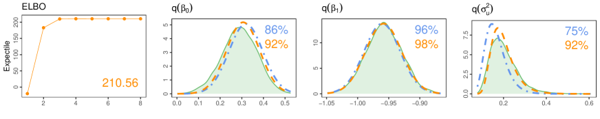
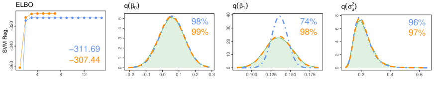
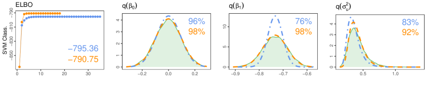
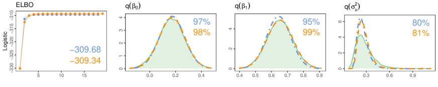
Figure 1: Comparison between MCMC (green), MFVB/Laplace (azure) and VMP (orange) in terms of evidence lower bound and marginal posterior approximation. Each row corresponds to a different model. The fist column shows the evidence lower bound for each iteration of MFVB and VMP. The other columns show the estimated marginal posterior densities for $\beta_{0}$, $\beta_{1}$ and $\sigma_{u}^{2}$ along with the associated accuracy scores for MFVB/Laplace and VMP.

We assess the quality of final variational approximations obtained via MFVB and VMP by calculating the average accuracy score for all the models in the simulation study described above. For a generic parameter $\theta$, the accuracy score is defined as

$$\text{Accuracy}\{q^{*}(\theta)\}=100\bigg{(}1-{\textstyle\frac{1}{2}}\,\int_{-\infty}^{+\infty}|\,q^{*}(\theta)-\pi(\theta|\mathbf{y})\,|\,\textrm{{d}}\theta\bigg{)}\%.$$ (20)

The true posterior density is here replaced by a kernel density estimate based on the MCMC samples from $\pi(\theta|\mathbf{y})$ and the integral is calculated via adaptive Gauss-Kronrod quadrature implemented in the Julia package QuadGK.

Figure 1 shows a comparison between the marginal posterior approximations of $\beta_{0}$, $\beta_{1}$ and $\sigma_{u}^{2}$ for MCMC, MFVB/Laplace and VMP. Additionally, it shows the evidence lower bound for each iteration of MFVB and VMP. Such approximations refer to the results obtained from one synthetic dataset in simulation setting B, where $n=500$ and $d=50$. In this scenario, VMP always reaches a higher evidence lower bound than MFVB, as predicted by Proposition 5. Moreover, VMP provides a better approximation of the marginal posteriors, in terms of accuracy score, while MFVB sometimes underestimates the posterior variance of $\beta_{1}$, as it happens for quantile regression, support vector regression and support vector classification.

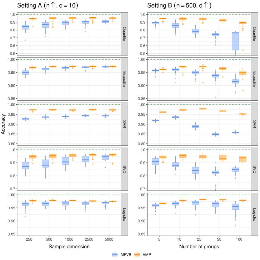
Figure 2: Sampling distribution of the average marginal accuracy score defined in (20) for the simulation setup described in Section 5.1. Each row corresponds to a model, each column corresponds to a simulation setting. The left column is for setting A, the right column is for setting B.

Figure 2 displays boxplots of the average accuracy scores, which are obtained by averaging the marginal accuracy scores over all the parameters in the model. At the increase of the sample size (setting A), the accuracy scores improve for all the considered approximations. The opposite happens when the sample size is kept fixed and the number of parameters grows (setting B). In both cases, we observe a uniform dominance of VMP over MFVB in all the simulation setups and for all the models considered in this study. Similarly, in the expectile regression case, VMP uniformly outperforms Laplace approximation in terms of accuracy. However, in the first simulation setting they are very close and tend to converge toward a steady-state accuracy value around $97.5\%$.

5.3 Computational efficiency

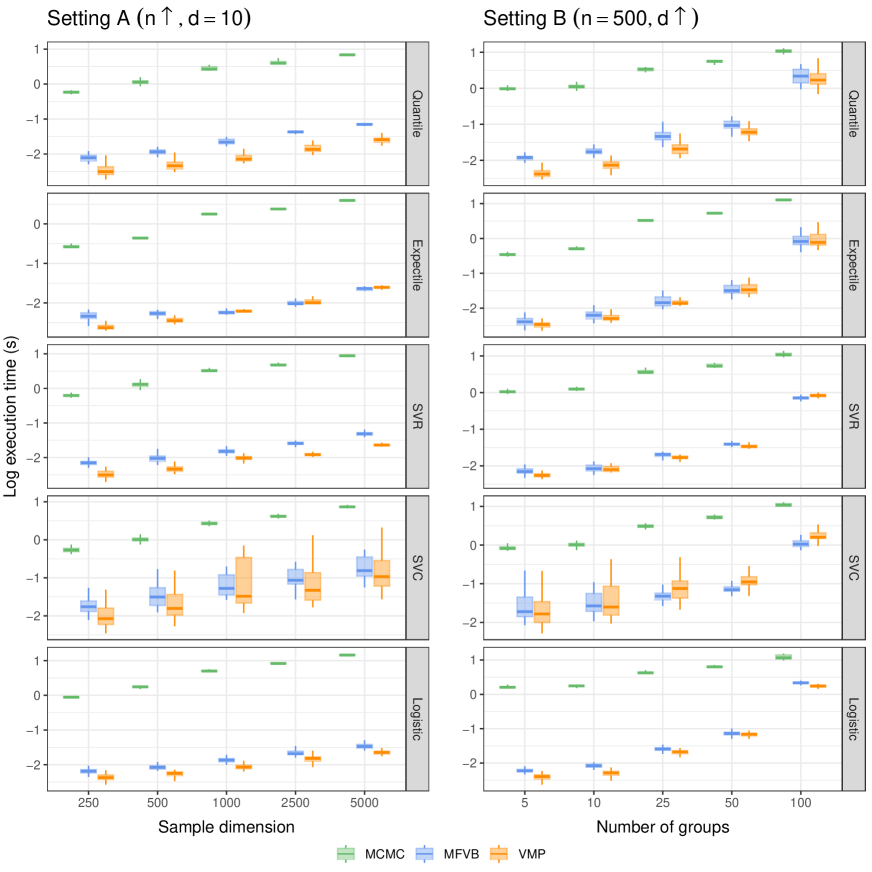
Figure 3: Sampling distribution of the $\log_{10}$-transformed execution time (in seconds) for the simulation setup described in Section 5.1. Each row corresponds to a model, each column corresponds to a simulation setting. The left column is for setting A, the right column is for setting B.

Figure 3 displays the $\log_{10}$-transformed computation times measured in seconds for MCMC, MFVB/Laplace and VMP. The execution time increases with the dimension of the problem, either in terms of sample size or number of random effect parameters. As we might expect, in all the considered scenarios, all the deterministic approximation methods yield a significant speed gain over MCMC in terms of execution time.

In simulation setting A, VMP yields a significant speed gain over MFVB for quantile, support vector and logistic regression. For expectile regression and support vector classification, VMP and MFVB/Laplace has similar performances on average, even though VMP is slightly more variable and always has a lower median execution time.

In simulation setting B, we observe a more balanced situation, where all the compared variational methods have similar execution times, even though VMP still provides some gains in the quantile and logistic regression examples.

Overall, we can conclude that MFVB/Laplace and VMP have the same computational complexity per iteration, similar execution times, but different performances in terms of posterior approximation accuracy, where VMP uniformly outperforms the competitors in terms of evidence lower bound and marginal approximation accuracy.

6 Real data applications

We here present four real data applications relative to distributional regression (Section 6.1), robust regression (Section 6.2) and unbalanced classification (Sections 6.3 adnd 6.4) tasks. We then discuss the results for all the applications in Section 6.5.

Likewise the simulations studies in Section 5, we estimate the true posterior via MCMC, and we approximate it via data augmented MFVB and non-conjugate VMP. In addition, we also consider the stochastic variational message passing method outlined in Algorithm 2, named sVMP. Doing so, we consider the learning rate schedule $\rho_{t}=\rho_{0}/(1+\rho_{0}\,t)^{3/4}$, which satisfy the Robbins-Monro conditions (Robbins and Monro,, 1951), where $\rho_{0}>0$ controls both the initial learning rate value and the decay speed to 0 of $\rho_{t}$ as $t$ diverges. In particular, in our experiments we set $\rho_{0}=0.05$ and we use minibatch samples with $100$ observations at each iteration of the algorithm. We run MCMC and sVMP for 10000 iterations, while MFVB and VMP are stopped when the relative change of the evidence lower bound falls below $10^{-6}$, with a maximum number of iterations set to 500. We set diffuse priors for all the parameters in the model, that is: $\sigma_{\beta}^{2}=10^{6}$, $A_{\varepsilon}=A_{h}=2.0001$, $B_{\varepsilon}=B_{h}=1.0001$.

To evaluate the computational efficiency and the posterior approximation quality of the considered methods, we report for each algorithm the number of iterations to convergence, the memory usage in GB, the execution time in seconds, the speed gain over MCMC, the average accuracy score and the evidence lower bound obtained at the end of the optimization. The speed gain over MCMC is calculated as the MCMC execution time divided by the execution time of the considered variational approximations, namely MFVB, VMP and sVMP.

All the references concerning the implementation of the MCMC and MFVB algorithms are provided in Table 2 of Section 5.

6.1 Power load consumption

The first dataset we examine has been utilized in the load forecasting track of the Global Energy Competition 2014 and is readily accessible in the supplementary material of Hong et al., (2016). This dataset comprises hourly load consumption and temperature data in the United States from January 2005 to December 2012, encompassing a total of 60600 observations. Previous studies conducted by Gaillard et al., (2016) and Fasiolo et al., (2021) have analyzed this dataset using additive quantile regression methods to predict the temporal evolution of power load consumption.

In this context, the data typically exhibit long-term non-stationary trends, multiple seasonal cycles of various amplitudes (e.g., daily, weekly, and monthly patterns), heteroscedasticity, and potential contamination from extreme values. Consequently, estimating multiple quantiles can provide a more comprehensive description of the data distribution than traditional mean regression.

Following the approaches of Gaillard et al., (2016) and Fasiolo et al., (2021), we model the $\tau$th quantile of load consumption as an additive function involving a long-term trend, daily, weekly, monthly, and yearly cycles, actual and smoothed temperature, as well as the lagged load consumption. We employ non-linear basis expansions for all covariates, employing cubic B-splines for non-periodic effects and Fourier bases for cyclic variables. As a result, each observation $y_{i}$ is associated with a 94-dimensional completed covariate vector $\mathbf{c}_{i}^{\top}$, where $i$ ranges from 1 to 60600. The coefficient vector $\boldsymbol{u}_{h}$ for each non-linear effect is treated as a random effect vector with its own variance parameter $\sigma_{h}^{2}$, where $h$ ranges from 1 to 8. To incorporate regularization, we utilize classical second-order differential penalization and construct the corresponding regularization matrix $\mathbf{R}_{h}$ for Fourier and B-spline basis coefficient vectors $\boldsymbol{u}_{h}$ (Wand and Ormerod,, 2008). Under this model specification, we estimate the unknown parameters for five quantile levels, specifically, $5\%$, $25\%$, $50\%$, $75\%$ and $95\%$, using MCMC, MFVB, VMP and sVMP. The results of such an analysis are reported in Table 3.

6.2 Beijing air quality

In the second application, we explore the Beijing PM2.5 dataset, which is freely available in the UCI machine learning repository (Chen,, 2017). This dataset comprises 43824 hourly measurements of PM2.5 concentration, collected by the US Embassy in Beijing from January 1st, 2010 to December 31st, 2014. It also includes 7 meteorological variables recorded at the Beijing Capital International Airport, namely dew point, temperature, pressure, combined wind direction, cumulated wind speed, cumulated hours of snow, and cumulated hours of rain. Additionally, the dataset provides information about the hour, day, month, and year of each measurement.

The objective of our analysis is to estimate the behavior of PM2.5 concentration in Beijing based on the available covariates. To achieve this, we employ a robust support vector regression model (Vapnik,, 1998) with an insensitivity parameter of $\epsilon=0.01$. We adopt an additive specification for the linear predictor, accounting for potential non-linear effects of the covariates using appropriate regularized Fourier and B-spline basis expansions. This yields a 140-dimensional completed vector $\mathbf{c}_{i}^{\top}$ for each observation $y_{i}$. Similar to the approach taken in Section 6.1, we model the $h$th basis coefficient vector $\boldsymbol{u}_{h}$ as a random effect vector, allowing it to have its own variance parameter $\sigma_{h}^{2}$, with $h$ ranging from $1$ to $11$. We then approximate the posterior using MCMC, MFVB, VMP and sVMP. The results are shown in Table 3.

6.3 Bank marketing

In the third application, we examine a bank marketing dataset obtained from the UCI machine learning repository (Moro et al.,, 2012). This dataset comprises 45211 instances involving various marketing campaigns conducted by a Portuguese banking institution. The objective of our analysis is to predict the likelihood of subscribing a financial product based on 17 covariates, including campaign descriptions, last contact reports, and client information such as age, job position, education, marital status, and financial position. Following necessary data preprocessing steps, such as dicotomization of categorical covariates and transformation of numeric variables, we obtain 48 predictors for our analysis.

We adopt a support vector classification model (Vapnik,, 1998) to predict the subscriptions, incorporating an adaptive ridge penalty on the regression parameters to mitigate overfitting. In this approach, we estimate the posterior distribution of the ridge regularization parameter from the available data, along with the other unknown coefficients.

Similar to previous analyses, we compare the estimated posterior distributions obtained via MCMC, MFVB VMP and sVMP, and we summarize the results in Table 3.

6.4 Forest cover types

For the fourth application, we consider the cover-type dataset provided by the UCI machine learning repository (Blackard,, 1998). It collects 581012 observations on forest cover-type and cartographic attributes measured on a $30\times 30$ meters grid from four wildness areas located in the Roosevelt National Forest of northern Colorado. The goal of the analysis is to predict the forest cover-type encoded in 7 categories given the elevation, aspect, slope, hillshade, soil-type and other topological features of the observed regions.

In this application, we predict the second category (lodgepole pine) against the others using a support vector machine classifier (Vapnik,, 1998) with a grouped ridge penalty, such that each group of covariates has its own shrinkage parameter. Doing so, we end up having a 52-dimensional vector of fixed and random effect covariates $\mathbf{c}_{i}^{\top}$, which is divided in 11 subgroups reflecting the structure of the grouped ridge penalty.

The results obtained by estimating the model with MCMC, MFVB, VMP and sVMP are reported in Table 3.

6.5 Numerical results

Table 3: Summary results for the applications described in Sections 6.1, 6.2, 6.3 and 6.4. From left to right column: approximation method, number of iterations, execution time in seconds (s), speed gain, average marginal accuracy, evidence lower bound.

Method	Iterations	Exe. time	Speed gain	Accuracy	ELBO
Power load consumption ($\tau=0.05$, $n=60600$, $p+d=94$)
MCMC	10000	436.64
MFVB	115	9.91	44.04	63.11 (13.37)	217656.12
VMP	19	2.71	161.00	96.63 (1.16)	217701.07
sVMP	10000	13.34	32.73	83.42 (13.79)	217689.83
Power load consumption ($\tau=0.25$, $n=60600$, $p+d=94$)
MCMC	10000	440.72
MFVB	54	4.95	88.87	70.74 (10.77)	144448.89
VMP	16	2.30	191.45	97.03 (1.56)	144481.36
sVMP	10000	13.01	33.88	88.23 (9.26)	144474.37
Power load consumption ($\tau=0.50$, $n=60600$, $p+d=94$)
MCMC	10000	438.49
MFVB	40	3.77	116.03	71.31 (10.65)	128322.37
VMP	16	2.31	189.74	96.73 (2.18)	128353.57
sVMP	10000	12.79	34.28	87.80 (8.42)	128347.20
Power load consumption ($\tau=0.75$, $n=60600$, $p+d=94$)
MCMC	10000	468.67
MFVB	59	5.97	78.38	70.35 (11.17)	141036.46
VMP	19	2.99	156.48	96.73 (2.11)	141069.37
sVMP	10000	13.26	35.34	87.57 (8.63)	141063.04
Power load consumption ($\tau=0.95$, $n=60600$, $p+d=94$)
MCMC	10000	487.68
MFVB	115	10.22	47.69	65.44 (13.17)	211368.35
VMP	19	2.86	170.10	96.74 (1.23)	211410.67
sVMP	10000	12.47	39.11	83.77 (13.97)	211395.47
Beijing air quality ($n=43824$, $p+d=140$)
MCMC	10000	559.36
MFVB	43	4.69	119.34	76.66 (12.74)	-6357.40
VMP	22	2.36	236.12	96.88 (1.62)	-6274.64
sVMP	10000	10.22	54.75	89.39 (8.48)	-6281.89
Bank marketing ($n=45211$, $p+d=48$)
MCMC	10000	121.69
MFVB	722	18.75	6.49	89.46 (14.66)	-504.91
VMP	68	2.24	54.33	95.50 (3.59)	-493.45
sVMP	10000	5.43	22.39	93.50 (7.12)	-495.27
Forest cover-type ($n=581012$, $p+d=52$)
MCMC	10000	2469.34
MFVB	128	39.81	62.02	55.96 (13.08)	-430.34
VMP	99	28.42	86.88	90.31 (16.61)	-430.31
sVMP	10000	9.56	258.30	75.05 (20.92)	-430.32

Table 3 presents the computational efficiency and posterior approximation accuracy results obtained in the four applications described so far. Among the considered approaches, the proposed batch non-conjugate variational message passing algorithm demonstrates excellent performance, exhibiting both a good efficiency and a superior accuracy. It converges rapidly and achieves a substantial speed gain over Markov chain Monte Carlo, conjugate mean field variational Bayes and stochastic variational message passing in the first three applications, while in the fourth one, it is the second fastest method after stochastic message passing outperforming Monte Carlo sampling and conjugate mean field approximation. In comparison to conjugate mean field variational Bayes and stochastic variational message passing, batch variational message passing showcases the highest average accuracy and evidence lower bound across all scenarios. Notably, it consistently surpasses $95\%$ accuracy in all settings, with minor deviations from the central value.

Conversely, stochastic variational message passing requires more iterations to converge, but, thanks to minibatch subsampling, each iteration is computationally cheaper than both mean field variational Bayes and non-conjugate variational message passing. Consequently, stochastic variational message passing exhibits favorable scalability, making it well-suited for handling massive data problems, where batch optimization would necessitate an impractical amount of memory to store the dataset and approximate the posterior distribution. Actually, in the forest cover-type application, which has the highest number of observations among the considered examples, stochastic message passing yields a substantial speed gain over Markov chain Monte Carlo, mean field variational Bayes and batch variational message passing.

Although the proposed stochastic method does not attain the same precision as batch variational message passing in terms of accuracy, it consistently achieves superior average accuracy and evidence lower bound compared to conjugate mean field variational Bayes. This behavior is not surprising, since the approximation obtained via stochastic optimization is, by definition, a noisy version of the deterministic approximation yielding from batch variational message passing. The precision of the proposed stochastic optimization technique thus depends on the amount of randomness injected in the algorithm via minibatch subsampling and by the number of iterations set before to stop the execution.

Overall, we can conclude that the proposed variational message passing methods are competitive with alternative conjugate mean field variational Bayes both in terms of computational speed and posterior approximation accuracy, systematically outperforming data-augmentation based approximations in all the simulation studies and real-data examples discussed in Sections 5 and 6.

7 Discussion and future extensions

We have developed a novel variational message passing method to estimate risk-based Bayesian regression models. Our approach is highly versatile and can be applied to a broad range of mixed regression models, which extends far beyond the limited examples we have presented in this work. By effectively addressing challenges associated with non-regular loss functions and non-conjugate priors, our method maintains a high level of efficiency while surpassing the accuracy of conjugate mean field variational Bayes in numerous instances. We have observed promising results in approximating the true target posterior distribution through both simulations and real-data examples.

This approach allows for several extensions and adaptations. For instance, specialized algorithms can be developed to handle models with multiple and nested random effects (Nolan et al.,, 2020; Menictas et al.,, 2023), dynamic linear models (Durbin and Koopman,, 2012; Triantafyllopoulos,, 2021), latent spatial fields (Rue et al.,, 2009; Lindgren et al.,, 2011), and inducing shrinkage priors (Carvalho et al.,, 2010; Armagan et al.,, 2013; Bhattacharya et al.,, 2015).

Frequentist mixed regression models can also be effectively addressed using a careful combination of expectation-maximization algorithms and Gaussian variational approximation, as demonstrated in studies such as Ormerod and Wand, (2010), Hall et al., 2011a , Hall et al., 2011b , Ormerod and Wand, (2012), Hui et al., (2019) and Westling and McCormick, (2019) among others. This approach presents a valuable alternative to cumbersome Monte Carlo integration (Geraci and Bottai,, 2007), multivariate quadrature methods (Geraci and Bottai,, 2014) and nested optimization (Geraci,, 2019) for models that lack the classical regularity conditions required for implementing the Laplace approximation. Exploring the use of variational methods for frequentist inferential purposes will be the focus of future research.

Another notable contribution of our work is the application of loss smoothing to address non-regular minimization problems. Loss smoothing is a commonly employed technique for optimizing non-smooth risk functions, involving the replacement of a non-regular loss with a tilted one. This substitution creates a new objective function that is uniformly differentiable throughout its domain, enabling the utilization of efficient optimization routines such as Newton and quasi-Newton algorithms. Examples of loss smoothing in the quantile regression literature can be found in the works of Hunter and Lange, (2000), Yue and Rue, (2011), Oh et al., (2011), and Fasiolo et al., (2021). Similar approaches have been considered in the support vector machines literature (Lee and Mangasarian,, 2001).

As demonstrated in Proposition 3, the variational loss averaging defined in formula (14) presents a novel method for constructing smooth majorizing objective functions from non-differentiable loss functions. Unlike other existing smoothing methods based on geometric considerations, our strategy is founded on statistical reasoning with a straightforward probabilistic interpretation, akin to the expectation-maximization algorithm. Furthermore, our proposal incorporates a practical rule to determine the local degree of smoothing induced by the approximation, which is determined by the posterior variance of the $i$-th linear predictor. This adaptive calibration of the new loss allows for distinct smoothing factors to be applied to each observation.

Appendix A Evidence lower bound and optimal distributions

Proof of Proposition 1

First, we consider the definition of the evidence lower bound (2), and we notice that it can be written in terms of a sum of expected values calculated with respect to the $q$-density as:

$$\underline{\ell}(\mathbf{y};q)=\int_{\Theta}q(\boldsymbol{\theta})\log\bigg{\{}\frac{\pi(\mathbf{y},\boldsymbol{\theta})}{q(\boldsymbol{\theta})}\bigg{\}}\,\textrm{{d}}\boldsymbol{\theta}=\mathbb{E}_{q}\{\log\pi(\mathbf{y},\boldsymbol{\theta})\}-\mathbb{E}_{q}\{\log q(\boldsymbol{\theta})\}$$

where $\log pi(\mathbf{y},\boldsymbol{\theta})=\log\pi(\mathbf{y}|\boldsymbol{\theta})+\log\pi(\boldsymbol{\theta})$. From the model specification (10) and (11), we have

$$\log\pi(\mathbf{y},\boldsymbol{\theta})=-\frac{n}{\phi}R_{n}(\boldsymbol{\theta})+\log\pi(\boldsymbol{\beta},\boldsymbol{u}|\sigma_{1}^{2},\dots,\sigma_{\scriptscriptstyle{H}}^{2})+\sum_{h=1}^{\scriptscriptstyle{H}}\log\pi(\sigma_{h}^{2})+\log\pi(\sigma_{\varepsilon}^{2}).$$

Similarly, thanks to the variational restriction (12) and (13), for the variational density we have:

$$\log q(\boldsymbol{\theta})=\log{q}(\boldsymbol{\beta},\boldsymbol{u})+\sum_{h=1}^{{\scriptscriptstyle{H}}}\log{q}(\sigma_{h}^{2})+\log{q}(\sigma_{\varepsilon}^{2}).$$

Therefore, the lower bound can be decomposed as a sum of terms associated to different parameter blocks:

$$\underline{\ell}(\mathbf{y};q)=\;\underbrace{-\frac{n}{\phi}\mathbb{E}_{q}\big{[}R_{n}(\boldsymbol{\theta})\big{]}}_{\textstyle T_{1}}+\underbrace{\mathbb{E}_{q}\bigg{[}\log\frac{\pi(\boldsymbol{\beta},\boldsymbol{u}|\boldsymbol{\sigma}_{u}^{2})}{q(\boldsymbol{\beta},\boldsymbol{u})}\bigg{]}}_{\textstyle T_{2}}+\sum_{h=1}^{{\scriptscriptstyle{H}}}\underbrace{\mathbb{E}_{q}\bigg{[}\log\frac{\pi(\sigma_{h}^{2})}{q(\sigma_{h}^{2})}\bigg{]}}_{\textstyle T_{3}}+\underbrace{\mathbb{E}_{q}\bigg{[}\log\frac{\pi(\sigma_{\varepsilon}^{2})}{q(\sigma_{\varepsilon}^{2})}\bigg{]}}_{\textstyle T_{4}}.$$ (21)

We can thus evaluate each term separately and sum up the individual contributions $T_{k}$, $k=1,\dots,4$.

The first term in (21) is the variational expectation of the risk function:

$$T_{1}=-\frac{n}{\phi}\mathbb{E}_{q}\big{[}R_{n}(\boldsymbol{\theta})\big{]}=-\frac{n}{\phi}\,\mathbb{E}_{q}(\log\sigma_{\varepsilon}^{2})-\frac{1}{\phi}\,\mathbb{E}_{q}(1/\sigma_{\varepsilon}^{2})\sum_{i=1}^{n}\mathbb{E}_{q}\{\psi_{0}(y_{i},\eta_{i})\}.$$

The second term in (21) is the expected contribution of $\boldsymbol{\vartheta}=(\boldsymbol{\beta},\boldsymbol{u})$ to the lower bound and corresponds to the negative Kullback-Leibler divergence between the multivariate Gaussian laws $\textrm{{N}}_{d}(\boldsymbol{\mu},\boldsymbol{\Sigma})$ and $\textrm{{N}}_{d}(\mathbf{0},\mathbf{S})$, where $\mathbf{S}=\textrm{{blockdiag}}\big{[}\sigma_{\beta}^{2}\mathbf{R}_{\beta}^{-1},\sigma_{1}^{2}\mathbf{R}_{1}^{-1},\dots,\sigma_{\scriptscriptstyle{H}}^{2}\mathbf{R}_{\scriptscriptstyle{H}}^{-1}\big{]}$:

$$T_{2} = \mathbb{E}_{q}\Big{[}-{\textstyle\frac{1}{2}}\,\textrm{{logdet}}(\mathbf{S})-{\textstyle\frac{1}{2}}\,\boldsymbol{\vartheta}^{\top}\mathbf{S}^{-1}\boldsymbol{\vartheta}+{\textstyle\frac{1}{2}}\,\textrm{{logdet}}(\boldsymbol{\Sigma})+{\textstyle\frac{1}{2}}\,(\boldsymbol{\vartheta}-\boldsymbol{\mu})^{\top}\boldsymbol{\Sigma}^{-1}(\boldsymbol{\vartheta}-\boldsymbol{\mu})\Big{]}$$

$$= -{\textstyle\frac{1}{2}}\,\mathbb{E}_{q}\big{[}\textrm{{logdet}}(\mathbf{S})\big{]}+{\textstyle\frac{1}{2}}\,\textrm{{logdet}}(\boldsymbol{\Sigma})-{\textstyle\frac{1}{2}}\,\mathbb{E}_{q}(\boldsymbol{\vartheta}^{\top}\mathbf{S}^{-1}\boldsymbol{\vartheta})+{\textstyle\frac{1}{2}}\,\mathbb{E}_{q}\big{[}(\boldsymbol{\vartheta}-\boldsymbol{\mu})^{\top}\boldsymbol{\Sigma}^{-1}(\boldsymbol{\vartheta}-\boldsymbol{\mu})\big{]}$$

$$= -{\textstyle\frac{1}{2}}\,\Big{[}d_{\beta}\log\sigma_{\beta}^{2}-\textrm{{logdet}}(\mathbf{R}_{\beta})\Big{]}-{\textstyle\frac{1}{2}}\,\sum_{h=1}^{\scriptscriptstyle{H}}\Big{[}d_{h}\mathbb{E}_{q}(\log\sigma_{h}^{2})-\textrm{{logdet}}(\mathbf{R}_{h})\Big{]}+{\textstyle\frac{1}{2}}\,\textrm{{logdet}}(\boldsymbol{\Sigma})$$

$$-{\textstyle\frac{1}{2}}\,(1/\sigma_{\beta}^{2})\Big{[}\boldsymbol{\mu}_{\beta}^{\top}\mathbf{R}_{\beta}\boldsymbol{\mu}_{\beta}+\textrm{{trace}}\big{(}\mathbf{R}_{\beta}\boldsymbol{\Sigma}_{\beta\beta}\big{)}\Big{]}+{\textstyle\frac{1}{2}}\,\sum_{h=1}^{\scriptscriptstyle{H}}\mathbb{E}_{q}(1/\sigma_{h}^{2})\Big{[}\boldsymbol{\mu}_{h}^{\top}\mathbf{R}_{h}\boldsymbol{\mu}_{h}+\textrm{{trace}}\big{(}\mathbf{R}_{h}\boldsymbol{\Sigma}_{hh}\big{)}\Big{]}+{\textstyle\frac{p+d}{2}\,}.$$

where we used the factorization (12) and the identity $\mathbb{E}_{q}\big{[}{(\boldsymbol{\vartheta}-\boldsymbol{\mu})}^{\top}\boldsymbol{\Sigma}^{-1}(\boldsymbol{\vartheta}-\boldsymbol{\mu})\big{]}=p+d$.

The third term in (21) is the expected contribution of $\sigma_{h}^{2}$ to the lower bound, which corresponds to the negative Kullback-Leibler divergence between the Inverse-Gamma distributions $\textrm{{IG}}(\alpha_{h},\beta_{h})$ and $\textrm{{IG}}(A_{h},B_{h})$:

$$T_{3} =\mathbb{E}_{q}\Big{[}A_{h}\log B_{h}-\log\Gamma(A_{h})-(A_{h}+1)\log\sigma_{h}^{2}-B_{h}/\sigma_{h}^{2}$$

$$\qquad-\alpha_{h}\log\beta_{h}+\log\Gamma(\alpha_{h})+(\alpha_{h}+1)\log\sigma_{h}^{2}+\beta_{h}/\sigma_{h}^{2}\Big{]}$$

$$=A_{h}\log(B_{h}/\beta_{h})-\log\big{\{}\Gamma(A_{h})/\Gamma(\alpha_{h})\big{\}}-(d_{h}/2)\big{\{}\log\beta_{h}-\mathbb{E}_{q}(\log\sigma_{h}^{2})\big{\}}-(B_{h}-\beta_{h})\,\mathbb{E}_{q}(1/\sigma_{h}^{2}),$$

where we used $\alpha_{h}=A_{h}+d_{h}/2$.

The fourth term in (21) is the expected contribution of $\sigma_{\varepsilon}^{2}$ to the lower bound, that corresponds to the negative Kullback-Leibler divergence between the Inverse-Gamma distributions $\textrm{{IG}}(\alpha_{\varepsilon},\beta_{\varepsilon})$ and $\textrm{{IG}}(A_{\varepsilon},B_{\varepsilon})$:

$$T_{4}=A_{\varepsilon}\log(B_{\varepsilon}/\beta_{\varepsilon})-\log\big{\{}\Gamma(A_{\varepsilon})/\Gamma(\alpha_{\varepsilon})\big{\}}-(n/\phi)\big{\{}\log\beta_{\varepsilon}-\mathbb{E}_{q}(\log\sigma_{\varepsilon}^{2})\big{\}}-(B_{\varepsilon}-\beta_{\varepsilon})\,\mathbb{E}_{q}(1/\sigma_{\varepsilon}^{2}),$$

where we used $\alpha_{\varepsilon}=A_{\varepsilon}+n/\phi$.

Finally, summing up the individual contributions $T_{1}$, $T_{2}$, $T_{3}$, $T_{4}$ and simplifying the redundant components, we obtain the result:

$$\underline{\ell}(\mathbf{y};q)= -\frac{1}{\phi}\,\mathbb{E}_{q}(1/\sigma_{\varepsilon}^{2})\sum_{i=1}^{n}\mathbb{E}_{q}\{\psi_{0}(y_{i},\eta_{i})\}-{\textstyle\frac{1}{2}}\,\Big{[}d_{\beta}\log\sigma_{\beta}^{2}-\textrm{{logdet}}(\mathbf{R}_{\beta})\Big{]}+{\textstyle\frac{1}{2}}\,\sum_{h=1}^{\scriptscriptstyle{H}}\textrm{{logdet}}(\mathbf{R}_{h})+{\textstyle\frac{1}{2}}\,\textrm{{logdet}}(\boldsymbol{\Sigma})$$

$$-{\textstyle\frac{1}{2}}\,(1/\sigma_{\beta}^{2})\Big{[}\boldsymbol{\mu}_{\beta}^{\top}\mathbf{R}_{\beta}\boldsymbol{\mu}_{\beta}+\textrm{{trace}}\big{(}\mathbf{R}_{\beta}\boldsymbol{\Sigma}_{\beta\beta}\big{)}\Big{]}+{\textstyle\frac{1}{2}}\,\sum_{h=1}^{\scriptscriptstyle{H}}\mathbb{E}_{q}(1/\sigma_{h}^{2})\Big{[}\boldsymbol{\mu}_{h}^{\top}\mathbf{R}_{h}\boldsymbol{\mu}_{h}+\textrm{{trace}}\big{(}\mathbf{R}_{h}\boldsymbol{\Sigma}_{hh}\big{)}\Big{]}$$

$$+\sum_{h=1}^{\scriptscriptstyle{H}}\Big{[}A_{h}\log(B_{h}/\beta_{h})-\log\big{\{}\Gamma(A_{h})/\Gamma(\alpha_{h})\big{\}}-(d_{h}/2)\log\beta_{h}-(B_{h}-\beta_{h})\,\mathbb{E}_{q}(1/\sigma_{h}^{2})\Big{]}$$

$$+A_{\varepsilon}\log(B_{\varepsilon}/\beta_{\varepsilon})-\log\big{\{}\Gamma(A_{\varepsilon})/\Gamma(\alpha_{\varepsilon})\big{\}}-(n/\phi)\log\beta_{\varepsilon}-(B_{\varepsilon}-\beta_{\varepsilon})\,\mathbb{E}_{q}(1/\sigma_{\varepsilon}^{2}).$$

The proof is concluded by noting that the second row in the formula above may be equivalently expressed as $\boldsymbol{\mu}^{\top}\bar{\mathbf{R}}\boldsymbol{\mu}+\textrm{{trace}}(\bar{\mathbf{R}}\boldsymbol{\Sigma})$ by defining the block-diagonal matrix $\bar{\mathbf{R}}=\textrm{{blockdiag}}\big{[}(1/\sigma_{\beta}^{2})\mathbf{R}_{\beta},\mathbb{E}_{q}(1/\sigma_{1}^{2})\mathbf{R}_{1},\dots,\mathbb{E}_{q}(1/\sigma_{\scriptscriptstyle{H}}^{2})\mathbf{R}_{\scriptscriptstyle{H}}\big{]}$. $\square$

Proof of Proposition 2

In this section we prove Proposition 2 and we derive the explicit solutions of the optimal variational distributions $q^{(t+1)}(\sigma_{\varepsilon}^{2})$, $q^{(t+1)}(\sigma_{u}^{2})$ and $q^{(t+1)}(\boldsymbol{\beta},\boldsymbol{u})$.

(a) Optimal distribution of $\sigma_{\varepsilon}^{2}$. We here leverage the equivalence between the natural gradient update in (4) and the exact variational message passing solution for mean field variational inference in conjugate exponential models (Equation 14, Tan and Nott,, 2013; Theorem 1, Khan and Lin,, 2017). Thus, we consider the optimal density $q^{(t+1)}(\sigma_{\varepsilon}^{2})\propto\exp\big{[}\mathbb{E}_{-\sigma_{\varepsilon}^{2}}^{(t)}\{\log\pi(\sigma_{\varepsilon}^{2}|\textup{rest})\}\big{]}$, where $\pi(\sigma_{\varepsilon}^{2}|\textup{rest})$ denotes the full-conditional distribution of $\sigma_{\varepsilon}^{2}$ and $\mathbb{E}_{-\sigma_{\varepsilon}^{2}}^{(t)}(\cdot)$ stands for the expected value calculated with respect to the density $q^{(t)}(\boldsymbol{\theta})/q^{(t)}(\sigma_{\varepsilon}^{2})$.

The full-conditional density function of $\sigma_{\varepsilon}^{2}$ is given by

$$\log\pi(\sigma_{\varepsilon}^{2}|\textup{rest})=-(A_{\varepsilon}+n/\phi+1)\log\sigma_{\varepsilon}^{2}-\bigg{[}B_{\varepsilon}+\frac{1}{\phi}\sum_{i=1}^{n}\mathbb{E}_{q}\{\psi_{0}(y_{i},\eta_{i})\}\bigg{]}/\sigma_{\varepsilon}^{2}+\textup{const},$$

which corresponds to the log kernel of an Inverse-Gamma distribution $\textrm{{IG}}(A_{\varepsilon|\bullet},B_{\varepsilon|\bullet})$, with parameters $A_{\varepsilon|\bullet}=A_{\varepsilon}+n/\phi$ and $B_{\varepsilon|\bullet}=B_{\varepsilon}+\sum_{i=1}^{n}\psi_{0}(y_{i},\eta_{i})/\phi$. Thus, taking the variational expectation of $\log\pi(\sigma_{\varepsilon}^{2}|\textup{rest})$ with respect to all the unknown parameters but $\sigma_{\varepsilon}^{2}$, we get

$$\log q^{(t+1)}(\sigma_{\varepsilon}^{2})=-(A_{\varepsilon}+n/\phi+1)\log\sigma_{\varepsilon}^{2}-\bigg{[}B_{\varepsilon}+\frac{1}{\phi}\sum_{i=1}^{n}\mathbb{E}_{q}^{(t)}\{\psi_{0}(y_{i},\eta_{i})\}\bigg{]}/\sigma_{\varepsilon}^{2}+\textup{const}.$$

The latter is the kernel of an Inverse-Gamma distribution with parameters $\alpha_{\varepsilon}^{(t+1)}=A_{\varepsilon}+n/\phi$ and $\beta_{\varepsilon}^{(t+1)}=B_{\varepsilon}+\sum_{i=1}^{n}\mathbb{E}_{q}^{(t)}\{\psi_{0}(y_{i},\eta_{i})\}/\phi$. This concludes the derivation of $q^{(t+1)}(\sigma_{\varepsilon}^{2})$.

(b) Optimal distribution of $\sigma_{h}^{2}$. Following the same mean field approach used in the derivation of $q^{(t+1)}(\sigma_{\varepsilon}^{2})$, we here derive the optimal density of $\sigma_{h}^{2}$ using the mean field solution $q^{(t+1)}(\sigma_{h}^{2})\propto\exp\big{[}\mathbb{E}_{-\sigma_{h}^{2}}\{\log\pi(\sigma_{h}^{2}|\textup{rest})\}\big{]}$.

Recalling that $\boldsymbol{u}_{h}|\sigma_{h}^{2}\sim\textrm{{N}}(\mathbf{0},\sigma_{h}^{2}\mathbf{R}_{h}^{-1})$ and $\sigma_{h}^{2}\sim\textrm{{IG}}(A_{h},B_{h})$, it is easy to show that the full-conditional log-density function of $\sigma_{h}^{2}$ is given By

$$\log\pi(\sigma_{h}^{2}|\textup{rest})=-(A_{h}+d_{h}/2+1)\log\sigma_{h}^{2}-\Big{\{}B_{h}+(\boldsymbol{u}_{h}^{\top}\mathbf{R}_{h}\,\boldsymbol{u}_{h})/2\Big{\}}/\sigma_{h}^{2}+\textup{const},$$

which corresponds to the log-kernel of an Inverse-Gamma distribution with parameters $A_{h|\bullet}=A_{h}+d_{h}/2$ and $B_{h|\bullet}=B_{h}+(\boldsymbol{u}_{h}^{\top}\mathbf{R}_{h}\,\boldsymbol{u}_{h})/2$. Thus, taking the variational expectation of $\log\pi(\sigma_{h}^{2}|\textup{rest})$ with respect to all the unknown parameters but $\sigma_{h}^{2}$, we get

$$\log q^{(t+1)}(\sigma_{h}^{2})=-(A_{h}+d_{h}/2+1)\log\sigma_{h}^{2}-\Big{\{}B_{h}+{\textstyle\frac{1}{2}}\,\mathbb{E}_{q}^{(t)}(\boldsymbol{u}_{h}^{\top}\mathbf{R}_{h}\,\boldsymbol{u}_{h})/2\Big{\}}/\sigma_{h}^{2}+\textup{const}.$$

The latter is the kernel of an Inverse-Gamma distribution with parameters $\alpha_{h}^{(t+1)}=A_{h}+d_{h}/2$ and $\beta_{h}^{(t+1)}=B_{h}+\mathbb{E}_{q}^{(t)}(\boldsymbol{u}_{h}^{\top}\mathbf{R}_{h}\,\boldsymbol{u}_{h})/2$. This concludes the derivation of $q^{(t+1)}(\sigma_{h}^{2})$.

(c) Optimal distribution of $(\boldsymbol{\beta},\boldsymbol{u})$. According to Proposition 1, the evidence lower bound (15) may be expressed as

$$\underline{\ell}(\mathbf{y};q,\boldsymbol{\mu},\boldsymbol{\Sigma}) =-\frac{1}{\phi}\mathbb{E}_{q}\{R_{n}(\boldsymbol{\theta})\}-\textrm{{KL}}\{q(\boldsymbol{\beta},\boldsymbol{u})\parallel\pi(\boldsymbol{\beta},\boldsymbol{u}|\boldsymbol{\sigma}_{u}^{2})\}+\textup{const}$$

$$=-\frac{\gamma_{\varepsilon}}{\phi}\sum_{i=1}^{n}\mathbb{E}_{q}\{\psi_{0}(y_{i},\eta_{i})\}+\frac{1}{2}\Big{\{}\textrm{{logdet}}(\boldsymbol{\Sigma})-\boldsymbol{\mu}^{\top}\bar{\mathbf{R}}\,\boldsymbol{\mu}-\textrm{{trace}}(\bar{\mathbf{R}}\boldsymbol{\Sigma})\Big{\}}+\textup{const},$$

where we discarded all the terms not depending on $\boldsymbol{\mu}$ and $\boldsymbol{\Sigma}$. Then, thanks to the Gaussian natural gradient update (6) by Wand, (2014), we may employ the recursion $\boldsymbol{\mu}^{(t+1)}\leftarrow\boldsymbol{\mu}^{(t)}-\big{[}\mathbf{H}^{(t)}\big{]}^{-1}\mathbf{g}^{(t)}$ and $\boldsymbol{\Sigma}^{(t+1)}\leftarrow-\big{[}\mathbf{H}^{(t)}\big{]}^{-1}$ to optimize the evidence lower bound with respect to $\boldsymbol{\mu}$ and $\boldsymbol{\Sigma}$. The gradient and Hessian of $\underline{\ell}(\mathbf{y};q,\boldsymbol{\mu},\boldsymbol{\Sigma})$ are

$$\mathbf{g}=-\frac{\gamma_{\varepsilon}}{\phi}\sum_{i=1}^{n}\frac{\partial}{\partial\boldsymbol{\mu}}\mathbb{E}_{q}\{\psi_{0}(y_{i},\eta_{i})\}-\bar{\mathbf{R}}\boldsymbol{\mu}\qquad\text{and}\qquad\mathbf{H}=-\frac{\gamma_{\varepsilon}}{\phi}\sum_{i=1}^{n}\frac{\partial^{2}}{\partial\boldsymbol{\mu}\,\partial\boldsymbol{\mu}^{\top}}\mathbb{E}_{q}\{\psi_{0}(y_{i},\eta_{i})\}-\bar{\mathbf{R}}.$$

We recall that the expected loss function may be written as

$$\Psi_{0}(y_{i},m_{i},\nu_{i})=\mathbb{E}_{q}\{\psi_{0}(y_{i},\eta_{i})\}=\int_{-\infty}^{+\infty}\psi_{0}(y_{i},\eta_{i})\,\phi(\eta_{i};m_{i},\nu_{i}^{2})\,\textrm{{d}}\eta_{i},$$

which depends on $\boldsymbol{\mu}$ and $\boldsymbol{\Sigma}$ only through the scalar variables $m_{i}=\mathbf{c}_{i}^{\top}\boldsymbol{\mu}$ and $\nu_{i}^{2}=\mathbf{c}_{i}^{\top}\boldsymbol{\Sigma}\,\mathbf{c}_{i}$. Therefore, thanks to the chain rule, we get

$$\frac{\partial\Psi_{0,i}}{\partial\boldsymbol{\mu}}=\frac{\partial m_{i}}{\partial\boldsymbol{\mu}}\frac{\partial\Psi_{0,i}}{\partial m_{i}}=\mathbf{c}_{i}\Psi_{1,i}\qquad\text{and}\qquad\frac{\partial^{2}\Psi_{0,i}}{\partial\boldsymbol{\mu}\,\partial\boldsymbol{\mu}^{\top}}=\frac{\partial m_{i}}{\partial\boldsymbol{\mu}}\frac{\partial m_{i}}{\partial\boldsymbol{\mu}^{\top}}\frac{\partial\Psi_{1,i}}{\partial m_{i}}=\mathbf{c}_{i}\mathbf{c}_{i}^{\top}\Psi_{2,i}.$$

Equivalently, in matrix form, we have $\mathbf{g}=-(\gamma_{\varepsilon}/\phi)\mathbf{C}^{\top}\boldsymbol{\Psi}_{1}-\bar{\mathbf{R}}\boldsymbol{\mu}$ and $\mathbf{H}=-(\gamma_{\varepsilon}/\phi)\mathbf{C}^{\top}\textrm{{diag}}(\boldsymbol{\Psi}_{2})\,\mathbf{C}-\bar{\mathbf{R}}$. This concludes the derivation of $q^{(t+1)}(\boldsymbol{\beta},\boldsymbol{u})$ and also the proof of Proposition 2. $\square$

Proof of Proposition 3

Let us assume that, for any $y\in\mathcal{Y}$, $\psi_{0}(y,\cdot):\mathbb{R}\rightarrow\mathbb{R}$ is a measurable function, having well-defined $r$th order weak derivative $\psi_{r}(y,\cdot)$, for $r=1,\dots,R$. Recall that the $r$th order weak derivative of $\psi_{0}(y,x)$ with respect to $x$, say $\psi_{r}(y,x)$, is defined as the integrable function satisfying the equation

$$\int_{a}^{b}\frac{\textrm{{d}}^{r}}{\textrm{{d}}{x}^{r}}\varphi(x)\,\psi_{0}(y,x)\,\textrm{{d}}{x}=(-1)^{r}\int_{a}^{b}\varphi(x)\,\psi_{r}(y,x)\,\textrm{{d}}{x},$$ (22)

for any infinitely differentiable test function $\varphi:[a,b]\rightarrow\mathbb{R}$ such that $\varphi(a)=\varphi(b)=0$.

We also recall that $\psi_{0}(y,x)$ is convex in $x$ if, and only if, $\psi_{2}(y,x)\geq 0$ almost everywhere. Moreover, if $\psi_{0}(y,x)$ is $r$ times differentiable in $x$, then $\psi_{r}(y,x)=(\partial^{r}/\partial x^{r})\psi_{0}(y,x)$.

(a) Differentiability. The differentiability of $\Psi_{0}(y,m,\nu)$ with respect to $m$ and $\nu$ is guaranteed by the derivation under integral sign theorem and by the fact that $\phi(\cdot;m,\nu^{2})$ is an analytic function having infinitely many continuous derivatives with respect to $m$ and $\nu$. In fact, since $\Psi_{0}(y,m,\nu)$ depends on $m$ and $\nu$ only through $\phi(\cdot;m,\nu^{2})$, we have

$$\frac{\partial^{\,r}}{\partial m^{r}}\frac{\partial^{\,s}}{\partial\nu^{s}}\int_{-\infty}^{+\infty}\psi_{0}(y,x)\,\phi(x;\mu,\nu^{2})\,\textrm{{d}}{x}=\int_{-\infty}^{+\infty}\psi_{0}(y,x)\frac{\partial^{\,r}}{\partial m^{r}}\frac{\partial^{\,s}}{\partial\nu^{s}}\,\phi(x;m,\nu^{2})\,\textrm{{d}}{x},$$ (23)

for any non-negative integer $r$ and $s$. Moreover, we observe that the right-hand side derivative may be written as $\nabla_{m}^{r}\nabla_{\nu}^{s}\,\phi(x;m,\nu)=p(x;m,\nu)\,\phi(x;m,\nu^{2})$, where $p(x;m,\nu)$ is a linear combination of Hermite polynomials of finite order parametrized by $m$ and $\nu$. Therefore, thanks to the Holder inequality, the right integral in (23) is bounded by

$$\bigg{|}\int_{-\infty}^{+\infty}\psi_{0}(y,x)\,p(x;m,\nu)\,\phi(x;m,\nu^{2})\,\textrm{{d}}{x}\bigg{|}\leq\int_{-\infty}^{+\infty}|\psi_{0}(y,x)\,p(x;m,\nu)|\,\phi(x;m,\nu^{2})\,\textrm{{d}}{x}$$

$$\leq\bigg{[}\int_{-\infty}^{+\infty}|\psi_{0}(y,x)|\,\phi(x;m,\nu^{2})\,\textrm{{d}}{x}\bigg{]}\bigg{[}\int_{-\infty}^{+\infty}|p(x;m,\nu)|\,\phi(x;m,\nu^{2})\,\textrm{{d}}{x}\bigg{]}<\infty$$

which is finite, since $\psi_{0}(y,x)$ is integrable and the moments of a Gaussian distribution are all well-defined for any $m\in\mathbb{R}$ and $\nu>0$. $\square$

(b) Convergence. Let $x_{t}\sim\textrm{{N}}(m,\nu_{t}^{2})$ be a sequence of random variables such that $\nu_{t}^{2}\rightarrow 0$ as $t\rightarrow\infty$. Then, thanks to the closure of the convergence in probability with respect to continuous transformations, if $\psi_{0}(y,x)$ is continuous in $x$, we get $\displaystyle\psi_{0}(y,x_{t})\;\mathop{\rightarrow}^{\textrm{{p}}}\;\psi_{0}(y,m)$ since $\displaystyle x_{t}\;\mathop{\rightarrow}^{\textrm{{p}}}\;m$. Hence, $\Psi_{0}(y,m,\nu)=\mathbb{E}\{\psi_{0}(y,x_{t})\}\rightarrow\psi_{0}(y,m)$ pointwise as $t\rightarrow\infty$. Moreover, by the continuity of $\psi_{0}$ and $\Psi_{0}$, we have $\sup_{m\in\mathbb{R}}\big{|}\Psi_{0}(y,m,\nu)-\psi_{0}(y,m)\big{|}\rightarrow 0$ uniformly for any $y\in\mathcal{Y}$. $\square$

(c) Joint convexity. We recall that convex functions are closed with respect to convolution with positive measures. More formally, if $f(u,v)$ is a convex function in $u$ for any $v$ and if $w(v)$ is a non-negative weighting function of $v$, the integral transformation $g(u)=\int_{-\infty}^{+\infty}f(u,v)\,w(v)\,\textrm{{d}}{v}$ is convex in $u$ (provided the integral exists); see, e.g., Lange, (2013), Chapter 6. Then, writing

$$\Psi_{0}(y,m,\nu)=\mathbb{E}_{q}\{\psi_{0}(y,\eta)\}=\int_{-\infty}^{+\infty}\psi_{0}(y,m+\nu z)\,\phi(z)\,\textrm{{d}}{z},$$

the convexity of $\Psi_{0}(y,m,\nu)$ immediately follows from the linearity of $m+\nu z$ and the convexity of $\psi_{0}(y,\eta)$ with respect to $\eta$. $\square$

(d) Majorization. The lower bound $\psi_{0}(y,m)\leq\Psi_{0}(y,m,\nu)$ immediately follows from the convexity of $\psi_{0}$ and the Jensen inequality: $\psi_{0}\{y,\mathbb{E}(x)\}\leq\mathbb{E}\{\psi_{0}(y,x)\}=\Psi_{0}\{y,\mathbb{E}(x),\mathbb{V}\textrm{{ar}}(x)\}$. $\square$

(e) Differentiation rule. Let consider the Gaussian random variable $x\sim\textrm{{N}}(m,\nu^{2})$, such that

$$\Psi_{0}(y,m,\nu)=\mathbb{E}\{\psi_{0}(y,x)\}=\int_{-\infty}^{+\infty}\,\psi_{0}(y,x)\,\phi(x;m,\nu^{2})\,\textrm{{d}}{x}.$$

In order to prove the identity $(\partial^{r}/\partial m^{r})\,\mathbb{E}\{\psi_{0}(y,x)\}=\mathbb{E}\{\psi_{r}(y,x)\}$, for any $r=1,\dots,R$, we use an induction argument. Let us start from the initial step deriving under integral sign with respect to $m$:

$$\frac{\partial\Psi_{0}}{\partial m}=\int_{-\infty}^{+\infty}\frac{\psi_{0}(y,x)}{\nu}\frac{\partial}{\partial m}\phi\bigg{(}\frac{x-m}{\nu}\bigg{)}\,\textrm{{d}}{x}\\ =-\frac{1}{\nu}\int_{-\infty}^{+\infty}\,\frac{\psi_{0}(y,x)}{\nu}\,\accentset{\mbox{\large.}}{\phi}\bigg{(}\frac{x-m}{\nu}\bigg{)}\,\textrm{{d}}{x}.$$

To lighten the notation, here and elsewhere, we adopt the time-derivative notation $\accentset{\mbox{\large.}}{\phi}(z)=\textrm{{d}}\phi/\textrm{{d}}{z}$. Because of the location-scale representation of the Gaussian distribution, we write $\displaystyle x=m+\nu\,z$, where $z\sim\textrm{{N}}(0,1)$ and $\displaystyle\textrm{{d}}{x}=\nu\,\textrm{{d}}{z}$; in this way, we have

$$\frac{\partial\Psi_{0}}{\partial m}=-\frac{1}{\nu}\int_{-\infty}^{+\infty}\,\psi_{0}(y,m+\nu z)\,\accentset{\mbox{\large.}}{\phi}(z)\,\textrm{{d}}{z}.$$

Observing that $\accentset{\mbox{\large.}}{\phi}(z)$ vanishes in the limit as $|z|\rightarrow\infty$ for any $r$, we are allowed to integrate by parts with respect to $z$, to apply the definition of weak derivative of $\psi_{0}$, and finally to reparametrize back to $x$, obtaining

$$\frac{\partial\Psi_{0}}{\partial m}=\int_{-\infty}^{+\infty}\,\psi_{1}(y,m+\nu z)\,\phi(z)\,\textrm{{d}}{z}=\int_{-\infty}^{+\infty}\,\psi_{1}(y,x)\,\phi(x;m,\nu)\,\textrm{{d}}{x}=\mathbb{E}\{\psi_{1}(y,x)\},$$

where, thanks to the chain rule, $\textrm{{d}}\psi_{0}(y,m+\nu z)=\psi_{1}(y,m+\nu z)\,\nu\,\textrm{{d}}{z}$. Such a result satisfy the identity in 3(e) for $r=1$, hence the initial step is concluded.

Let us move to the induction step. We consider the $r$th order derivative of $\Psi_{0}$, namely $\Psi_{r}$, and we differentiate again under integral sign with respect to $m$:

$$\frac{\partial}{\partial m}\frac{\partial^{r}\Psi_{0}}{\partial m^{r}}=\frac{\partial\Psi_{r}}{\partial m}=\int_{-\infty}^{+\infty}\psi_{r}(y,x)\frac{\partial}{\partial m}\phi(x;m,\nu^{2})\,\textrm{{d}}{x}.$$

Following the same arguments used before, sequentially applying derivation, location-scale transformation, integration by parts and back-transformation, we get

$$\frac{\partial\Psi_{r}}{\partial m} =\int_{-\infty}^{+\infty}\frac{\psi_{r}(y,x)}{\nu}\frac{\partial}{\partial m}\phi\bigg{(}\frac{x-m}{\nu}\bigg{)}\,\textrm{{d}}{x}=-\frac{1}{\nu}\int_{-\infty}^{+\infty}\frac{\psi_{r}(y,x)}{\nu}\accentset{\mbox{\large.}}{\phi}\bigg{(}\frac{x-m}{\nu}\bigg{)}\,\textrm{{d}}{x}$$

$$=-\frac{1}{\nu}\int_{-\infty}^{+\infty}\psi_{r}(y,m+\nu\,z)\,\accentset{\mbox{\large.}}{\phi}(z)\,\textrm{{d}}{z}=\int_{-\infty}^{+\infty}\psi_{r+1}(y,m+\nu\,z)\,\phi(z)\,\textrm{{d}}{z}$$

$$=\int_{-\infty}^{+\infty}\psi_{r+1}(y,x)\,\phi(x;m,\nu^{2})=\mathbb{E}\{\psi_{r+1}(y,x)\}.$$

This concludes the induction step and also the proof. $\square$

Appendix B $\Psi$-function derivation

We here derive the explicit expressions of the $\Psi$-functions shown in Table 1. To do so, we first define $\delta_{0}$ as the Dirac delta function at $0$, we denote $x\sim\textrm{{N}}(\mu,\nu^{2})$ the generic Gaussian random variable with mean $\mu\in\mathbb{R}$ and variance $\nu^{2}>0$ and we set the non random constants $a,b\in\mathbb{R}$ and $c>0$. Then, we recall the following identities:

$$\mathbb{E}\{\delta_{0}(x)\} =\phi(0;\mu,\nu^{2}),$$ (24)

$$\mathbb{E}\{\textrm{{sign}}(x)\} =1-2\Phi(0;\mu,\nu^{2}),$$ (25)

$$\mathbb{E}(|x|) =\mu-2\mu\Phi(0;\mu,\nu^{2})+2\nu^{2}\phi(0;\mu,\nu^{2}),$$ (26)

$$\mathbb{E}\{x\,\mathbb{I}_{[a,b]}(x)\} =\mu\big{[}\Phi(b;\mu,\nu^{2})-\Phi(a;\mu,\nu^{2})\big{]}-\nu^{2}\big{[}\phi(b;\mu,\nu^{2})-\phi(a;\mu,\nu^{2})\big{]},$$ (27)

$$\mathbb{E}\{x^{2}\,\mathbb{I}_{[a,b]}(x)\} =(\mu^{2}+\nu^{2})\big{[}\Phi(b;\mu,\nu^{2})-\Phi(a;\mu,\nu^{2})\big{]}-2\nu^{2}\mu\big{[}\phi(b;\mu,\nu^{2})-\phi(a;\mu,\nu^{2})\big{]}$$ (28)

$$\qquad-\nu^{2}\big{[}(b-\mu)\phi(b;\mu,\nu^{2})-(a-\mu)\phi(a;\mu,\nu^{2})\big{]}.$$

Moreover, in the following derivations, we will make use of a simplified notation for the identity functions of left and right unbounded intervals, that is: $\mathbb{I}_{<b}(x)\equiv\mathbb{I}_{(-\infty,b]}(x)$ and $\mathbb{I}_{>a}(x)\equiv\mathbb{I}_{[a,+\infty)}(x)$.

Support vector classification. By the definition of Hinge loss function $\psi(y,\eta)=\psi(1-y\eta)=2\max(0,1-y\eta)$, we may write

$$\psi_{0}(x) =2\max(0,x)=|x|+(x),$$

$$\psi_{1}(x) =-y\,\textrm{{sign}}(x)-y=-2y\big{[}1-\mathbb{I}_{<0}(x)\big{]},$$

$$\psi_{2}(x) =2\delta_{0}(x)$$

where $x=1-y\eta\sim\textrm{{N}}(\mu,\nu^{2})$, with $\mu=1-ym$. Then, defining $\Phi_{0}=\Phi(0;\mu,\nu^{2})$ and $\phi_{0}=\phi(0;\mu,\nu^{2})$, taking the expectation and using (26) and (25), we get

$$\mathbb{E}\{\psi_{0}(x)\} =\mathbb{E}\,|x|+\mathbb{E}(x)=2\mu(1-\Phi_{0})+2\nu^{2}\phi_{0},$$

$$\mathbb{E}\{\psi_{1}(x)\} =-2y\big{[}1-\,\mathbb{E}\{\mathbb{I}_{<0}(x)\}\big{]}=-2y(1-\Phi_{0}),$$

$$\mathbb{E}\{\psi_{2}(x)\} =2\,\mathbb{E}\{\delta_{0}(x)\}=2\,\phi_{0}.$$

This concludes the derivation.

Support vector regression. By the definition of $\epsilon$-insensitive loss function $\psi(y,\eta)=\psi(y-\eta)=\max(0,|y-\eta|-\epsilon)$, we may write

$$\psi_{0}(x) ={\textstyle\frac{1}{2}}\,|x-\epsilon|+{\textstyle\frac{1}{2}}\,(x-\epsilon)+{\textstyle\frac{1}{2}}\,|y-\eta+\epsilon|-{\textstyle\frac{1}{2}}\,(y-\eta+\epsilon),$$

$$\psi_{1}(x) =-{\textstyle\frac{1}{2}}\,\textrm{{sign}}(x-\epsilon)-{\textstyle\frac{1}{2}}\,\textrm{{sign}}(x+\epsilon),$$

$$\psi_{2}(x) =2\delta_{0}(x-\epsilon)+2\delta_{0}(x+\epsilon),$$

where $x=y-\eta\sim\textrm{{N}}(\mu,\nu^{2})$, with $\mu=y-m$. Then, defining $\Phi_{\epsilon}^{+}=\Phi(\epsilon;\mu,\nu^{2})$, $\Phi_{\epsilon}^{-}=\Phi(-\epsilon;\mu,\nu^{2})$, $\phi_{\epsilon}^{+}=\phi(\epsilon;\mu,\nu^{2})$ and $\phi_{\epsilon}^{-}=\phi(-\epsilon;\mu,\nu^{2})$, and using identity (26), we have

$${\textstyle\frac{1}{2}}\,\mathbb{E}\,|x-\epsilon|+{\textstyle\frac{1}{2}}\,\mathbb{E}(x-\epsilon) =(y-m-\epsilon)(1-\Phi_{\epsilon}^{-})+\nu^{2}\phi_{\epsilon}^{-},$$

$${\textstyle\frac{1}{2}}\,\mathbb{E}\,|x+\epsilon|-{\textstyle\frac{1}{2}}\,\mathbb{E}(x+\epsilon) =(y-m+\epsilon)(1-\Phi_{\epsilon}^{+})+\nu^{2}\phi_{\epsilon}^{+},$$

and $\mathbb{E}\{\psi_{0}(x)\}={\textstyle\frac{1}{2}}\,\big{[}\mathbb{E}\,|x-\epsilon|+\mathbb{E}(x-\epsilon)+\mathbb{E}\,|x+\epsilon|-\mathbb{E}(x+\epsilon)\big{]}$. Similarly, using (25), we have

$$\mathbb{E}\{\psi_{1}(x)\} =-{\textstyle\frac{1}{2}}\,\mathbb{E}\{\textrm{{sign}}(x-\epsilon)\}-{\textstyle\frac{1}{2}}\,\mathbb{E}\{\textrm{{sign}}(x+\epsilon)\}=\Phi_{\epsilon}^{+}+\Phi_{\epsilon}^{-}-1,$$

$$\mathbb{E}\{\psi_{2}(x)\} =\mathbb{E}\{\delta_{0}(x-\epsilon)\}+2\,\mathbb{E}\{\delta_{0}(x+\epsilon)\}=\phi_{\epsilon}^{+}+\phi_{\epsilon}^{-}.$$

This concludes the derivation.

Quantile regression. By the definition of quantile check loss $\psi(y,\eta)=\psi(y-\eta)=(y-\eta)[\tau-\mathbb{I}_{\leq 0}(y-\eta)]$, we may write

$$\psi_{0}(x) ={\textstyle\frac{1}{2}}\,|x|+(\tau-{\textstyle\frac{1}{2}}\,)(x),$$

$$\psi_{1}(x) =-{\textstyle\frac{1}{2}}\,\textrm{{sign}}(x)-(\tau-{\textstyle\frac{1}{2}}\,),$$

$$\psi_{2}(x) =\delta_{0}(x),$$

where $x=y-\eta\sim\textrm{{N}}(\mu,\nu^{2})$, with $\mu=y-m$. Then, defining $\Phi_{0}=\Phi(0;\mu,\nu^{2})$ and $\phi_{0}=\phi(0;\mu,\nu^{2})$, taking the expectation and using (26) and (25), we get

$$\mathbb{E}\big{\{}\psi_{0}(x)\big{\}} ={\textstyle\frac{1}{2}}\,\mathbb{E}(|x|)+(\tau-{\textstyle\frac{1}{2}}\,)\mathbb{E}(x)=\mu(\tau-\Phi_{0})+\nu^{2}\,\phi_{0},$$

$$\mathbb{E}\big{\{}\psi_{1}(x)\big{\}} =-{\textstyle\frac{1}{2}}\,\mathbb{E}\{\textrm{{sign}}(x)\}-(\tau-{\textstyle\frac{1}{2}}\,)=\Phi_{0}-\tau,$$

$$\mathbb{E}\big{\{}\psi_{2}(x)\big{\}} =\mathbb{E}\{\delta_{0}(x)\}=\phi_{0}.$$

This concludes the derivation.

Expectile regression. By the definition of expectile loss $\psi(y,\eta)=\psi(y-\eta)={\textstyle\frac{1}{2}}\,(y-\eta)^{2}|\tau-\mathbb{I}_{\leq 0}(y-\eta)|$, we may write

$$\psi_{0}(x) ={\textstyle\frac{1}{2}}\,x^{2}\big{[}\tau+(1-2\tau)\mathbb{I}_{<0}(x)\big{]},$$

$$\psi_{1}(x) =-x\big{[}\tau+(1-2\tau)\mathbb{I}_{<0}(x)\big{]},$$

$$\psi_{2}(x) =\tau+(1-2\tau)\,\mathbb{I}_{<0}(x),$$

where $x=y-\eta\sim\textrm{{N}}(y-m,\nu^{2})$, with $\mu=y-m$. Then, defining $\Phi_{0}=\Phi(0;\mu,\nu^{2})$ and $\phi_{0}=\phi(0;\mu,\nu^{2})$, taking the expectation and using (28), we have

$$\mathbb{E}\{\psi_{0}(x)\} ={\textstyle\frac{1}{2}}\,\tau\mathbb{E}\{(x)^{2}\}+{\textstyle\frac{1}{2}}\,(1-2\tau)\,\mathbb{E}\{(x)^{2}\,\mathbb{I}_{<0}(x)\}$$

$$={\textstyle\frac{1}{2}}\,\tau(\mu^{2}+\nu^{2})+{\textstyle\frac{1}{2}}\,(1-2\tau)\big{[}(\mu^{2}+\nu^{2})\Phi_{0}-\mu\nu^{2}\phi_{0}\big{]}$$

$$={\textstyle\frac{1}{2}}\,(\mu^{2}+\nu^{2})\big{[}\tau+(1-2\tau)\Phi_{0}\big{]}-{\textstyle\frac{1}{2}}\,(1-2\tau)\mu\nu^{2}\phi_{0}.$$

In the same way, using (27), we get

$$\mathbb{E}\{\psi_{1}(x)\} =-\tau\mathbb{E}(x)-(1-2\tau)\,\mathbb{E}\{(x)\,\mathbb{I}_{<0}(x)\}$$

$$=-\mu\big{[}\tau+(1-2\tau)\Phi_{0}\big{]}+(1-2\tau)\nu^{2}\phi_{0},$$

and

$$\mathbb{E}\{\psi_{2}(x)\}=\tau+(1-2\tau)\,\mathbb{E}\{\mathbb{I}_{<0}(x)\}=\tau+(1-2\tau)\,\Phi_{0}.$$

This concludes the derivation.

Huber regression. By the definition of Huber regression loss, we may write $\psi(y,\eta)=\psi(y-\eta)$ so that

$$\psi_{0}(x) ={\textstyle\frac{1}{2\epsilon}\,}x^{2}\mathbb{I}_{\leq\epsilon}(|x|)-x\mathbb{I}_{<-\epsilon}(x)+x\mathbb{I}_{>\epsilon}(x)-{\textstyle\frac{\epsilon}{2}\,}[\mathbb{I}_{<-\epsilon}(x)+\mathbb{I}_{>\epsilon}(x)],$$

$$\psi_{1}(x) =-{\textstyle\frac{1}{\epsilon}\,}x\,\mathbb{I}_{\leq\epsilon}(|x|)-\mathbb{I}_{<-\epsilon}(x)+\mathbb{I}_{>\epsilon}(x),$$

$$\psi_{2}(x) ={\textstyle\frac{1}{\epsilon}\,}\mathbb{I}_{\leq\epsilon}(|x|),$$

where $x=y-\eta\sim\textrm{{N}}(\mu,\nu^{2})$, with $\mu=y-m$. Then, defining $\Phi_{\epsilon}^{+}=\Phi(\epsilon;\mu,\nu^{2})$, $\Phi_{\epsilon}^{-}=\Phi(-\epsilon;\mu,\nu^{2})$, $\phi_{\epsilon}^{+}=\phi(\epsilon;\mu,\nu^{2})$ and $\phi_{\epsilon}^{-}=\phi(-\epsilon;\mu,\nu^{2})$, and using identities (27) and (28), we get

$$\mathbb{E}\{\psi_{0}(x)\}= {\textstyle\frac{1}{2}}\,(\mu^{2}+\nu^{2})(\Phi_{\epsilon}^{+}-\Phi_{\epsilon}^{-})-\nu^{2}\mu(\phi_{\epsilon}^{+}-\phi_{\epsilon}^{-})-{\textstyle\frac{1}{2}}\,\nu^{2}\big{[}(\epsilon-\mu)\phi_{\epsilon}^{+}+(\epsilon+\mu)\phi_{\epsilon}^{-}\big{]}$$ (29)

$$-\epsilon\big{[}\mu\Phi_{\epsilon}^{-}-\nu^{2}\phi_{\epsilon}^{-}\big{]}+\epsilon\big{[}\mu(1-\Phi_{\epsilon}^{+})+\nu^{2}\phi_{\epsilon}^{+}\big{]}-{\textstyle\frac{1}{2}}\,\epsilon^{2}(\Phi_{\epsilon}^{-}+1-\Phi_{\epsilon}^{+}).$$

In the same way, we use (27) to find the expectations of $\psi_{1}(x)$ and $\psi_{2}(x)$

$$\mathbb{E}\{\psi_{1}(x)\} =-\mu(\Phi_{\epsilon}^{+}-\Phi_{\epsilon}^{-})+\nu^{2}(\phi_{\epsilon}^{+}-\phi_{\epsilon}^{-})+\epsilon(\Phi_{\epsilon}^{+}+\Phi_{\epsilon}^{-})-\epsilon,$$

$$\mathbb{E}\{\psi_{2}(x)\} =\Phi_{\epsilon}^{+}-\Phi_{\epsilon}^{-}.$$

This concludes the derivation.

Huber classification. By the definition of Huber classification loss, we may write $\psi(y,\eta)=\psi(1-y\eta)$ so that

$$\psi_{0}(x) ={\textstyle\frac{1}{4\epsilon}\,}(\epsilon+x)^{2}\,\mathbb{I}_{\leq\epsilon}(|x|)+(x)\mathbb{I}_{>\epsilon}(1-y\eta),$$

$$\psi_{1}(x) =-{\textstyle\frac{1}{2\epsilon}\,}y(\epsilon+x)\,\mathbb{I}_{\leq\epsilon}(|x|)-y\,\mathbb{I}_{>\epsilon}(x),$$

$$\psi_{2}(x) ={\textstyle\frac{1}{2\epsilon}\,}\mathbb{I}_{\leq\epsilon}(|x|),$$

where $x=1-y\eta\sim\textrm{{N}}(\mu,\nu^{2})$, with $\mu=1-ym$. Then, defining $\Phi_{\epsilon}^{+}=\Phi(\epsilon;\mu,\nu^{2})$, $\Phi_{\epsilon}^{-}=\Phi(-\epsilon;\mu,\nu^{2})$, $\phi_{\epsilon}^{+}=\phi(\epsilon;\mu,\nu^{2})$ and $\phi_{\epsilon}^{-}=\phi(-\epsilon;\mu,\nu^{2})$, and using identities (27) and (28), we get

$$\mathbb{E}\{\psi_{0}(x)\}= {\textstyle\frac{1}{4\epsilon}\,}\mathbb{E}\{x^{2}\mathbb{I}_{\leq\epsilon}(|x|)\}+{\textstyle\frac{1}{2}\,}\mathbb{E}\{x\mathbb{I}_{\leq\epsilon}(|x|)\}+{\textstyle\frac{\epsilon}{4}\,}\mathbb{E}\{\mathbb{I}_{\leq\epsilon}(|x|)\}+\mathbb{E}\{x\mathbb{I}_{>\epsilon}(x)\}$$ (30)

$$= {\textstyle\frac{1}{4\epsilon}\,}\big{[}(\mu^{2}+\nu^{2})(\Phi_{\epsilon}^{+}-\Phi_{\epsilon}^{-})-y\mu\nu^{2}(\phi_{\epsilon}^{+}-\phi_{\epsilon}^{-})-\epsilon\nu^{2}(\phi_{\epsilon}^{+}+\phi_{\epsilon}^{-})\big{]}$$

$$-{\textstyle\frac{1}{2}\,}\big{[}y\mu(\Phi_{\epsilon}^{+}+\Phi_{\epsilon}^{-})-\nu(\phi_{\epsilon}^{+}+\phi_{\epsilon}^{-})\big{]}+{\textstyle\frac{\epsilon}{4}\,}(\Phi_{\epsilon}^{+}-\Phi_{\epsilon}^{-}).$$

In the same way, we use (27) to find the expectations of $\psi_{1}(y,\eta)$ and $\psi_{2}(y,\eta)$

$$\mathbb{E}\{\psi_{1}(x)\} =-{\textstyle\frac{y}{2\epsilon}\,}\big{[}\mu(\Phi_{\epsilon}^{+}-\Phi_{\epsilon}^{-})-\nu^{2}(\phi_{\epsilon}^{+}-\phi_{\epsilon}^{-})\big{]}-{\textstyle\frac{y}{2}\,}(2-\Phi_{\epsilon}^{+}-\Phi_{\epsilon}^{-}),$$

$$\mathbb{E}\{\psi_{2}(x)\} ={\textstyle\frac{1}{2\epsilon}\,}(\Phi_{\epsilon}^{+}-\Phi_{\epsilon}^{-}).$$

This concludes the derivation.

Appendix C Marginal and augmented variational inference

Proof of Proposition 4

Let $q(\boldsymbol{\omega},\boldsymbol{\theta})=q(\boldsymbol{\omega}|\boldsymbol{\theta})q(\boldsymbol{\theta})$ be any density function over the parameter space $\Omega\times\Theta$, then we may write the Kullback-Leibler divergence between $q(\boldsymbol{\omega},\boldsymbol{\theta})$ and $\pi(\boldsymbol{\omega},\boldsymbol{\theta}|\mathbf{y})$ as follows

$$\textrm{{KL}}\{q(\boldsymbol{\omega},\boldsymbol{\theta})\parallel\pi(\boldsymbol{\omega},\boldsymbol{\theta}|\mathbf{y})\} =\textrm{{KL}}\{q(\boldsymbol{\omega}|\boldsymbol{\theta})\,q(\boldsymbol{\theta})\parallel\pi(\boldsymbol{\omega}|\boldsymbol{\theta},\mathbf{y})\,\pi(\boldsymbol{\theta}|\mathbf{y})\}$$

$$=-\iint_{\Theta\times\Omega}q(\boldsymbol{\omega}|\boldsymbol{\theta})\,q(\boldsymbol{\theta})\log\bigg{\{}\frac{\pi(\boldsymbol{\omega}|\boldsymbol{\theta},\mathbf{y})\,\pi(\boldsymbol{\theta}|\mathbf{y})}{q(\boldsymbol{\omega}|\boldsymbol{\theta})\,q(\boldsymbol{\theta})}\bigg{\}}\,\textrm{{d}}\boldsymbol{\theta}\,\textrm{{d}}\boldsymbol{\omega}$$

$$=-\int_{\Theta}q(\boldsymbol{\theta})\bigg{[}\int_{\Omega}q(\boldsymbol{\omega}|\boldsymbol{\theta})\log\bigg{\{}\frac{\pi(\boldsymbol{\omega}|\boldsymbol{\theta},\mathbf{y})}{q(\boldsymbol{\omega}|\boldsymbol{\theta})}\bigg{\}}\,\textrm{{d}}\boldsymbol{\omega}\bigg{]}\,\textrm{{d}}\boldsymbol{\theta}-\int_{\Theta}q(\boldsymbol{\theta})\log\bigg{\{}\frac{\pi(\boldsymbol{\theta}|\mathbf{y})}{q(\boldsymbol{\theta})}\bigg{\}}\,\textrm{{d}}\boldsymbol{\theta}$$

$$=\int_{\Theta}q(\boldsymbol{\theta})\,\textrm{{KL}}\{q(\boldsymbol{\omega}|\boldsymbol{\theta})\parallel\pi(\boldsymbol{\omega}|\boldsymbol{\theta},\mathbf{y})\}\,\textrm{{d}}\boldsymbol{\theta}+\textrm{{KL}}\{q(\boldsymbol{\theta})\parallel\pi(\boldsymbol{\theta}|\mathbf{y})\}$$

$$=\underbrace{\mathbb{E}_{q}\big{[}\textrm{{KL}}\{q(\boldsymbol{\omega}|\boldsymbol{\theta})\parallel\pi(\boldsymbol{\omega}|\boldsymbol{\theta},\mathbf{y})\}\big{]}}_{\geq 0}\;+\;\underbrace{\textrm{{KL}}\{q(\boldsymbol{\theta})\parallel\pi(\boldsymbol{\theta}|\mathbf{y})\}}_{\geq 0}.$$

Notice that the first term nullifies if and only if $\textrm{{KL}}\{q(\boldsymbol{\omega}|\boldsymbol{\theta})\parallel\pi(\boldsymbol{\omega}|\boldsymbol{\theta},\mathbf{y})\}=0$ for almost every $\boldsymbol{\theta}\in\Theta$, while the second term corresponds to the Kullback-Leibler divergence calculated over the marginal posterior distribution of $\boldsymbol{\theta}$, which does not depend on $q(\boldsymbol{\omega}|\boldsymbol{\theta})$. The optimal posterior approximation of $\pi(\boldsymbol{\omega},\boldsymbol{\theta}|\mathbf{y})$ is then the solution of the following variational problem

$$\min_{q(\boldsymbol{\theta})\in\mathcal{Q}_{\scriptscriptstyle\textrm{{M}}},q(\boldsymbol{\omega}|\boldsymbol{\theta})\in\mathcal{Q}_{\scriptscriptstyle\textrm{{C}}}}\mathbb{E}_{q}\big{[}\textrm{{KL}}\{q(\boldsymbol{\omega}|\boldsymbol{\theta})\parallel\pi(\boldsymbol{\omega}|\boldsymbol{\theta},\mathbf{y})\}\big{]}+\textrm{{KL}}\{q(\boldsymbol{\theta})\parallel\pi(\boldsymbol{\theta}|\mathbf{y})\}$$

$$\quad=\min_{q(\boldsymbol{\theta})\in\mathcal{Q}_{\scriptscriptstyle\textrm{{M}}}}\bigg{[}\min_{q(\boldsymbol{\omega}|\boldsymbol{\theta})\in\mathcal{Q}_{\scriptscriptstyle\textrm{{C}}}}\mathbb{E}_{q}\big{[}\textrm{{KL}}\{q(\boldsymbol{\omega}|\boldsymbol{\theta})\parallel\pi(\boldsymbol{\omega}|\boldsymbol{\theta},\mathbf{y})\}\big{]}+\textrm{{KL}}\{q(\boldsymbol{\theta})\parallel\pi(\boldsymbol{\theta}|\mathbf{y})\}\bigg{]}$$

which involve a first profiling with respect to $q(\boldsymbol{\omega}|\boldsymbol{\theta})\in\mathcal{Q}_{\scriptscriptstyle\textrm{{C}}}$ and then an external optimization with respect to $q(\boldsymbol{\theta})\in\mathcal{Q}_{\scriptscriptstyle\textrm{{M}}}$. Therefore, denoting by $q_{\scriptscriptstyle\textrm{{A}}}^{*}(\boldsymbol{\omega}|\boldsymbol{\theta})\in\mathcal{Q}_{\scriptscriptstyle\textrm{{C}}}$ the optimal approximation of $\pi(\boldsymbol{\omega}|\boldsymbol{\theta},\mathbf{y})$ for any $\boldsymbol{\theta}\in\Theta$, which is the minimizer of $\mathbb{E}_{q}\big{[}\textrm{{KL}}\{q(\boldsymbol{\omega}|\boldsymbol{\theta})\parallel\pi(\boldsymbol{\omega}|\boldsymbol{\theta},\mathbf{y})\}\big{]}$, we obtain

$$q_{\scriptscriptstyle\textrm{{A}}}^{*}(\boldsymbol{\theta})=\mathop{\textrm{{argmin}}}_{q(\boldsymbol{\theta})\in\mathcal{Q}_{\scriptscriptstyle\textrm{{M}}}}\;\textrm{{KL}}\{q(\boldsymbol{\theta})\parallel\pi(\boldsymbol{\theta}|\mathbf{y})\}+\mathbb{E}_{q}\big{[}\textrm{{KL}}\{q_{\scriptscriptstyle\textrm{{A}}}^{*}(\boldsymbol{\omega}|\boldsymbol{\theta})\parallel\pi(\boldsymbol{\omega}|\boldsymbol{\theta},\mathbf{y})\}\big{]}.$$

This concludes the proof of Proposition 4. $\square$

Proof of Proposition 5

The first scenario we consider is $\pi(\boldsymbol{\omega}|\boldsymbol{\theta},\mathbf{y})\in\mathcal{Q}_{\scriptscriptstyle\textrm{{C}}}$. In this case, thanks to the fundamental properties of the Kullback-Leibler divergence (Kullback and Leibler,, 1951) and to Proposition 4, the unique solution $q_{\scriptscriptstyle\textrm{{A}}}^{*}(\boldsymbol{\omega}|\boldsymbol{\theta})$ is given by

$$q_{\scriptscriptstyle\textrm{{A}}}^{*}(\boldsymbol{\omega}|\boldsymbol{\theta}) =\mathop{\textrm{{argmin}}}_{q(\boldsymbol{\omega}|\boldsymbol{\theta})\in\mathcal{Q}_{\scriptscriptstyle\textrm{{C}}}}\mathbb{E}_{q}\big{[}\textrm{{KL}}\{q(\boldsymbol{\omega}|\boldsymbol{\theta})\parallel\pi(\boldsymbol{\omega}|\boldsymbol{\theta},\mathbf{y})\}\big{]}$$

$$=\mathop{\textrm{{argmin}}}_{q(\boldsymbol{\omega}|\boldsymbol{\theta})\in\mathcal{Q}_{\scriptscriptstyle\textrm{{C}}}}\textrm{{KL}}\{q(\boldsymbol{\omega}|\boldsymbol{\theta})\parallel\pi(\boldsymbol{\omega}|\boldsymbol{\theta},\mathbf{y})\}=\pi(\boldsymbol{\omega}|\boldsymbol{\theta},\mathbf{y}),$$

since the Kullback-Leibler divergence is strictly convex with respect to $q(\boldsymbol{\omega}|\boldsymbol{\theta})$ and $q_{\scriptscriptstyle\textrm{{A}}}^{*}(\boldsymbol{\omega}|\boldsymbol{\theta})=\pi(\boldsymbol{\omega}|\boldsymbol{\theta},\mathbf{y})$ is the only density function such that $\textrm{{KL}}\{q_{\scriptscriptstyle\textrm{{A}}}^{*}(\boldsymbol{\omega}|\boldsymbol{\theta})\parallel\pi(\boldsymbol{\omega}|\boldsymbol{\theta},\mathbf{y})\}=0$, for any $\boldsymbol{\theta}\in\Theta$. As a consequence, the optimal variational approximation of $\pi(\boldsymbol{\theta}|\mathbf{y})$ is the solution of

$$q_{\scriptscriptstyle\textrm{{A}}}^{*}(\boldsymbol{\theta}) =\mathop{\textrm{{argmin}}}_{q(\boldsymbol{\theta})\in\mathcal{Q}_{\scriptscriptstyle\textrm{{M}}}}\textrm{{KL}}\{q(\boldsymbol{\theta})\parallel\pi(\boldsymbol{\theta}|\mathbf{y})\}+\mathbb{E}_{q}\big{[}\textrm{{KL}}\{q_{\scriptscriptstyle\textrm{{A}}}^{*}(\boldsymbol{\omega}|\boldsymbol{\theta})\parallel\pi(\boldsymbol{\omega}|\boldsymbol{\theta},\mathbf{y})\}\big{]}$$

$$=\mathop{\textrm{{argmin}}}_{q(\boldsymbol{\theta})\in\mathcal{Q}_{\scriptscriptstyle\textrm{{M}}}}\textrm{{KL}}\{q(\boldsymbol{\theta})\parallel\pi(\boldsymbol{\theta}|\mathbf{y})\}=q_{\scriptscriptstyle\textrm{{M}}}^{*}(\boldsymbol{\theta}),$$

which, by definition, leads to $q_{\scriptscriptstyle\textrm{{A}}}^{*}(\boldsymbol{\theta})=q_{\scriptscriptstyle\textrm{{M}}}^{*}(\boldsymbol{\theta})$ almost everywhere. The equality of the Kullback-Leibler divergences in (19) directly follows from the correspondence between $q_{\scriptscriptstyle\textrm{{A}}}^{*}(\boldsymbol{\theta})$ and $q_{\scriptscriptstyle\textrm{{M}}}^{*}(\boldsymbol{\theta})$ and by the global optimality of $q_{\scriptscriptstyle\textrm{{A}}}^{*}(\boldsymbol{\omega}|\boldsymbol{\theta})=\pi(\boldsymbol{\omega}|\boldsymbol{\theta},\mathbf{y})$. The resulting approximation for $\pi(\boldsymbol{\omega},\boldsymbol{\theta}|\mathbf{y})$ then corresponds to $q_{\scriptscriptstyle\textrm{{A}}}^{*}(\boldsymbol{\omega},\boldsymbol{\theta})=\pi(\boldsymbol{\omega}|\boldsymbol{\theta},\mathbf{y})\,q_{\scriptscriptstyle\textrm{{A}}}^{*}(\boldsymbol{\theta})$. This concludes the first part of the proof.

The second scenario we consider is $\pi(\boldsymbol{\omega}|\boldsymbol{\theta},\mathbf{y})\neq\mathcal{Q}_{\scriptscriptstyle\textrm{{C}}}$. In this case, $\textrm{{KL}}\{q(\boldsymbol{\omega}|\boldsymbol{\theta})\parallel\pi(\boldsymbol{\omega}|\boldsymbol{\theta},\mathbf{y})\}>0$ for any $q(\boldsymbol{\omega}|\boldsymbol{\theta})\in\mathcal{Q}_{\scriptscriptstyle\textrm{{C}}}$ and $\boldsymbol{\theta}\in\Theta$, in fact $q_{\scriptscriptstyle\textrm{{A}}}^{*}(\boldsymbol{\omega}|\boldsymbol{\theta})\neq\pi(\boldsymbol{\omega}|\boldsymbol{\theta},\mathbf{y})$ almost everywhere. As a consequence, the optimal distribution $q_{\scriptscriptstyle\textrm{{A}}}^{*}(\boldsymbol{\theta})$ is the solution of the regularized variational problem in (17). By strict convexity and by definition of global minimum, $\textrm{{KL}}\{q_{\scriptscriptstyle\textrm{{M}}}^{*}(\boldsymbol{\theta})\parallel\pi(\boldsymbol{\theta}|\mathbf{y})\}\leq\textrm{{KL}}\{\bar{q}(\boldsymbol{\theta})\parallel\pi(\boldsymbol{\theta}|\mathbf{y})\}$ for any $\bar{q}(\boldsymbol{\theta})\in\mathcal{Q}_{\scriptscriptstyle\textrm{{M}}}$. In particular, the inequality holds for $\bar{q}(\boldsymbol{\theta})=q_{\scriptscriptstyle\textrm{{A}}}^{*}(\boldsymbol{\theta})$, and

$$\textrm{{KL}}\{q_{\scriptscriptstyle\textrm{{M}}}^{*}(\boldsymbol{\theta})\parallel\pi(\boldsymbol{\theta}|\mathbf{y})\}\leq\textrm{{KL}}\{q_{\scriptscriptstyle\textrm{{A}}}^{*}(\boldsymbol{\theta})\parallel\pi(\boldsymbol{\theta}|\mathbf{y})\}<\textrm{{KL}}\{q_{\scriptscriptstyle\textrm{{A}}}^{*}(\boldsymbol{\theta})\parallel\pi(\boldsymbol{\theta}|\mathbf{y})\}+\mathbb{E}_{q_{\scriptscriptstyle\textrm{{A}}}^{*}}\big{[}\textrm{{KL}}\{q_{\scriptscriptstyle\textrm{{A}}}^{*}(\boldsymbol{\omega}|\boldsymbol{\theta})\parallel\pi(\boldsymbol{\omega}|\boldsymbol{\theta},\mathbf{y})\}\big{]}.$$

This concludes the proof of Proposition 5. $\square$

Remark 2.

The key assumption in Proposition 5 is that $q_{\scriptscriptstyle\textrm{{M}}}^{*}(\boldsymbol{\theta})$ and $q_{\scriptscriptstyle\textrm{{A}}}^{*}(\boldsymbol{\theta})$ belong in the same functional space $\mathcal{Q}_{\scriptscriptstyle\textrm{{M}}}$. Whenever such a compatibility assumption is not satisfied there are no guaranties that Proposition 5 holds true. In the following we show this fact by using a counterexample.

Example 2.

Let us consider a generic augmented space $\mathcal{Q}_{\scriptscriptstyle\textrm{{A}}}$ such that $\pi(\boldsymbol{\omega},\boldsymbol{\theta}|\mathbf{y})\in\mathcal{Q}_{\scriptscriptstyle\textrm{{A}}}$. On the opposite, we consider $\mathcal{Q}_{\scriptscriptstyle\textrm{{M}}}$ such that $\pi(\boldsymbol{\theta}|\mathbf{y})\notin\mathcal{Q}_{\scriptscriptstyle\textrm{{M}}}$. This way, $\mathcal{Q}_{\scriptscriptstyle\textrm{{A}}}$ and $\mathcal{Q}_{\scriptscriptstyle\textrm{{M}}}$ are not compatible by construction, since there exists at least one element of $\mathcal{Q}_{\scriptscriptstyle\textrm{{A}}}$ whose marginal density does not belong to $\mathcal{Q}_{\scriptscriptstyle\textrm{{M}}}$, namely $\pi(\boldsymbol{\theta}|\mathbf{y})=\int_{\Omega}\pi(\boldsymbol{\omega},\boldsymbol{\theta})\,\textrm{{d}}\boldsymbol{\omega}$. Recall that the Kullback-Leibler divergence is always non-negative, i.e. $\textrm{{KL}}(q\parallel\pi)\geq 0$, and reaches 0 if and only if $q=\pi$ almost everywhere, namely $\textrm{{KL}}(\pi\parallel\pi)=0$. Then, there exists at least one element of $\mathcal{Q}_{\scriptscriptstyle\textrm{{A}}}$ such that $\textrm{{KL}}\{q_{\scriptscriptstyle\textrm{{A}}}(\boldsymbol{\omega},\boldsymbol{\theta})\parallel\pi(\boldsymbol{\omega},\boldsymbol{\theta}|\mathbf{y})\}=0$, which corresponds to $q_{\scriptscriptstyle\textrm{{A}}}(\boldsymbol{\omega},\boldsymbol{\theta})=\pi(\boldsymbol{\omega},\boldsymbol{\theta}|\mathbf{y})$, whereas $\textrm{{KL}}\{q_{\scriptscriptstyle\textrm{{M}}}(\boldsymbol{\theta})\parallel\pi(\boldsymbol{\theta}|\mathbf{y})\}>0$ for any $q_{\scriptscriptstyle\textrm{{M}}}(\boldsymbol{\theta})\in\mathcal{Q}_{\scriptscriptstyle\textrm{{M}}}$, since $\pi(\boldsymbol{\theta}|\mathbf{y})\notin\mathcal{Q}_{\scriptscriptstyle\textrm{{M}}}$. This means that

$$\underbrace{\textrm{{KL}}\{q_{\scriptscriptstyle\textrm{{M}}}(\boldsymbol{\theta})\parallel\pi(\boldsymbol{\theta}|\mathbf{y})\}}_{\textstyle>0}\;\nleq\;\underbrace{\textrm{{KL}}\{\pi(\boldsymbol{\omega},\boldsymbol{\theta}|\mathbf{y})\parallel\pi(\boldsymbol{\omega},\boldsymbol{\theta}|\mathbf{y})\}}_{\textstyle=0},\qquad\forall\,q_{\scriptscriptstyle\textrm{{M}}}(\boldsymbol{\theta})\in\mathcal{Q}_{\scriptscriptstyle\textrm{{M}}},$$

which contradicts the inequality in Proposition 5.

References

• Albert and Chib, (1993) Albert, J. H. and Chib, S. (1993). Bayesian analysis of binary and polychotomous response data. J. Amer. Statist. Assoc., 88(422):669–679.
• Amari, (1998) Amari, S.-I. (1998). Natural gradient works efficiently in learning. Neural computation, 10(2):251–276.
• Armagan et al., (2013) Armagan, A., Dunson, D. B., and Lee, J. (2013). Generalized double Pareto shrinkage. Statist. Sinica, 23(1):119–143.
• Azzalini and Dalla Valle, (1996) Azzalini, A. and Dalla Valle, A. (1996). The multivariate skew-normal distribution. Biometrika, 83(4):715–726.
• Bhattacharya et al., (2015) Bhattacharya, A., Pati, D., Pillai, N. S., and Dunson, D. B. (2015). Dirichlet-Laplace priors for optimal shrinkage. J. Amer. Statist. Assoc., 110(512):1479–1490.
• Bishop, (2006) Bishop, C. M. (2006). Pattern recognition and machine learning. Information Science and Statistics. Springer, New York.
• Bissiri et al., (2016) Bissiri, P. G., Holmes, C. C., and Walker, S. G. (2016). A general framework for updating belief distributions. J. R. Stat. Soc. Ser. B. Stat. Methodol., 78(5):1103–1130.
• Blackard, (1998) Blackard, J. (1998). Covertype. UCI Machine Learning Repository. DOI: https://doi.org/10.24432/C50K5N.
• Blei et al., (2017) Blei, D. M., Kucukelbir, A., and McAuliffe, J. D. (2017). Variational inference: A review for statisticians. J. Amer. Statist. Assoc., 112(518):859–877.
• Bonnet, (1964) Bonnet, G. (1964). Transformations des signaux aléatoires à travers les systèmes non linéaires sans mémoire. Ann. Télécommun., 19:203–220.
• Carvalho et al., (2010) Carvalho, C. M., Polson, N. G., and Scott, J. G. (2010). The horseshoe estimator for sparse signals. Biometrika, 97(2):465–480.
• Chen, (2017) Chen, S. (2017). Beijing PM2.5 Data. UCI Machine Learning Repository. DOI: https://doi.org/10.24432/C5JS49.
• Degani et al., (2022) Degani, E., Maestrini, L., Toczydł owska, D., and Wand, M. P. (2022). Sparse linear mixed model selection via streamlined variational Bayes. Electron. J. Stat., 16(2):5182–5225.
• Dempster et al., (1977) Dempster, A. P., Laird, N. M., and Rubin, D. B. (1977). Maximum likelihood from incomplete data via the EM algorithm. J. Roy. Statist. Soc. Ser. B, 39(1):1–38.
• Duan et al., (2018) Duan, L. L., Johndrow, J. E., and Dunson, D. B. (2018). Scaling up data augmentation MCMC via calibration. J. Mach. Learn. Res., 19:Paper No. 64, 34.
• Durante and Rigon, (2019) Durante, D. and Rigon, T. (2019). Conditionally conjugate mean-field variational Bayes for logistic models. Statist. Sci., 34(3):472–485.
• Durbin and Koopman, (2012) Durbin, J. and Koopman, S. J. (2012). Time series analysis by state space methods, volume 38 of Oxford Statistical Science Series. Oxford University Press, Oxford, second edition.
• Fasano et al., (2022) Fasano, A., Durante, D., and Zanella, G. (2022). Scalable and accurate variational Bayes for high-dimensional binary regression models. Biometrika, 109(4):901–919.
• Fasiolo et al., (2021) Fasiolo, M., Wood, S. N., Zaffran, M., Nedellec, R., and Goude, Y. (2021). Fast calibrated additive quantile regression. J. Amer. Statist. Assoc., 116(535):1402–1412.
• Gaillard et al., (2016) Gaillard, P., Goude, Y., and Nedellec, R. (2016). Additive models and robust aggregation for gefcom2014 probabilistic electric load and electricity price forecasting. Int. J. Forecast., 32(3):1038–1050.
• Gelman et al., (2013) Gelman, A., Carlin, J. B., Stern, H. S., Dunson, D. B., Vehtari, A., and Rubin, D. B. (2013). Bayesian data analysis, third edition. CRC press.
• Geraci, (2019) Geraci, M. (2019). Modelling and estimation of nonlinear quantile regression with clustered data. Comput. Statist. Data Anal., 136:30–46.
• Geraci and Bottai, (2007) Geraci, M. and Bottai, M. (2007). Quantile regression for longitudinal data using the asymmetric Laplace distribution. Biostatistics, 8(1):140–154.
• Geraci and Bottai, (2014) Geraci, M. and Bottai, M. (2014). Linear quantile mixed models. Stat. Comput., 24(3):461–479.
• Germain et al., (2016) Germain, P., Bach, F., Lacoste, A., and Lacoste-Julien, S. (2016). PAC-Bayesian theory meets Bayesian inference. Advances in Neural Information Processing Systems, 29.
• (26) Hall, P., Ormerod, J. T., and Wand, M. P. (2011a). Theory of Gaussian variational approximation for a Poisson mixed model. Statist. Sinica, 21(1):369–389.
• (27) Hall, P., Pham, T., Wand, M. P., and Wang, S. S. J. (2011b). Asymptotic normality and valid inference for Gaussian variational approximation. Ann. Statist., 39(5):2502–2532.
• Hoffman et al., (2013) Hoffman, M. D., Blei, D. M., Wang, C., and Paisley, J. (2013). Stochastic variational inference. J. Mach. Learn. Res., 14:1303–1347.
• Hong et al., (2016) Hong, T., Pinson, P., Fan, S., Zareipour, H., Troccoli, A., and Hyndman, R. J. (2016). Probabilistic energy forecasting: Global energy forecasting competition 2014 and beyond. Int. J. Forecast., 32(3):896–913.
• Honkela et al., (2010) Honkela, A., Raiko, T., Kuusela, M., Tornio, M., and Karhunen, J. (2010). Approximate Riemannian conjugate gradient learning for fixed-form variational Bayes. J. Mach. Learn. Res., 11:3235–3268.
• Honkela et al., (2008) Honkela, A., Tornio, M., Raiko, T., and Karhunen, J. (2008). Natural conjugate gradient in variational inference. In Neural Information Processing: 14th International Conference, ICONIP 2007, Kitakyushu, Japan, November 13-16, 2007, Revised Selected Papers, Part II 14, pages 305–314. Springer.
• Hui et al., (2019) Hui, F. K. C., You, C., Shang, H. L., and Müller, S. (2019). Semiparametric regression using variational approximations. J. Amer. Statist. Assoc., 114(528):1765–1777.
• Hunter and Lange, (2000) Hunter, D. R. and Lange, K. (2000). Quantile regression via an MM algorithm. J. Comput. Graph. Statist., 9(1):60–77.
• Jaakkola and Jordan, (2000) Jaakkola, T. S. and Jordan, M. I. (2000). Bayesian parameter estimation via variational methods. Stat. Comput., 10(1):25–37.
• Johndrow et al., (2019) Johndrow, J. E., Smith, A., Pillai, N., and Dunson, D. B. (2019). MCMC for imbalanced categorical data. J. Amer. Statist. Assoc., 114(527):1394–1403.
• Khan and Lin, (2017) Khan, M. and Lin, W. (2017). Conjugate-computation variational inference: Converting variational inference in non-conjugate models to inferences in conjugate models. In Artificial Intelligence and Statistics, pages 878–887. PMLR.
• Khan and Nielsen, (2018) Khan, M. E. and Nielsen, D. (2018). Fast yet simple natural-gradient descent for variational inference in complex models. In 2018 International Symposium on Information Theory and Its Applications (ISITA), pages 31–35. IEEE.
• Khan et al., (2018) Khan, M. E., Nielsen, D., Tangkaratt, V., Lin, W., Gal, Y., and Srivastava, A. (2018). Fast and scalable bayesian deep learning by weight-perturbation in adam. In International conference on machine learning, pages 2611–2620. PMLR.
• Khan and Rue, (2021) Khan, M. E. and Rue, H. (2021). The bayesian learning rule. arXiv preprint arXiv:2107.04562.
• Knoblauch et al., (2022) Knoblauch, J., Jewson, J., and Damoulas, T. (2022). An optimization-centric view on Bayes’ rule: Reviewing and generalizing variational inference. J. Mach. Learn. Res., 23(1):5789–5897.
• Knowles and Minka, (2011) Knowles, D. and Minka, T. (2011). Non-conjugate variational message passing for multinomial and binary regression. Advances in Neural Information Processing Systems, 24:1701–1709.
• Koenker, (2005) Koenker, R. (2005). Quantile regression, volume 38 of Econometric Society Monographs. Cambridge University Press, Cambridge.
• Kotz et al., (2001) Kotz, S., Kozubowski, T. J., and Podgórski, K. (2001). The Laplace distribution and generalizations. A revisit with applications to communications, economics, engineering, and finance. Birkhäuser Boston, Inc., Boston, MA.
• Kozumi and Kobayashi, (2011) Kozumi, H. and Kobayashi, G. (2011). Gibbs sampling methods for Bayesian quantile regression. J. Stat. Comput. Simul., 81(11):1565–1578.
• Kucukelbir et al., (2017) Kucukelbir, A., Tran, D., Ranganath, R., Gelman, A., and Blei, D. M. (2017). Automatic differentiation variational inference. J. Mach. Learn. Res., 18:Paper No. 14, 45.
• Kullback and Leibler, (1951) Kullback, S. and Leibler, R. A. (1951). On information and sufficiency. Ann. Math. Statistics, 22:79–86.
• Lange, (2013) Lange, K. (2013). Optimization. Springer, New York, second edition.
• Lange et al., (1989) Lange, K. L., Little, R. J. A., and Taylor, J. M. G. (1989). Robust statistical modeling using the $t$ distribution. J. Amer. Statist. Assoc., 84(408):881–896.
• Lee and Mangasarian, (2001) Lee, Y.-J. and Mangasarian, O. L. (2001). SSVM: a smooth support vector machine for classification. Comput. Optim. Appl., 20(1):5–22.
• Lewandowski et al., (2010) Lewandowski, A., Liu, C., and Wiel, S. V. (2010). Parameter expansion and efficient inference. Statistical Science, 25(4):533 – 544.
• Lin et al., (2019) Lin, W., Khan, M. E., and Schmidt, M. (2019). Fast and simple natural-gradient variational inference with mixture of exponential-family approximations. In International Conference on Machine Learning, pages 3992–4002. PMLR.
• (52) Lin, W., Nielsen, F., Khan, M. E., and Schmidt, M. (2021a). Structured second-order methods via natural gradient descent. arXiv preprint arXiv:2107.10884.
• (53) Lin, W., Nielsen, F., Khan, M. E., and Schmidt, M. (2021b). Tractable structured natural-gradient descent using local parameterizations. In International Conference on Machine Learning, pages 6680–6691. PMLR.
• Lindgren et al., (2011) Lindgren, F., Rue, H., and Lindström, J. (2011). An explicit link between Gaussian fields and Gaussian Markov random fields: the stochastic partial differential equation approach. J. R. Stat. Soc. Ser. B Stat. Methodol., 73(4):423–498.
• Liu and Pierce, (1994) Liu, Q. and Pierce, D. A. (1994). A note on Gauss-Hermite quadrature. Biometrika, 81(3):624–629.
• Loaiza-Maya et al., (2022) Loaiza-Maya, R., Smith, M. S., Nott, D. J., and Danaher, P. J. (2022). Fast and accurate variational inference for models with many latent variables. J. Econometrics, 230(2):339–362.
• Luts and Ormerod, (2014) Luts, J. and Ormerod, J. T. (2014). Mean field variational Bayesian inference for support vector machine classification. Comput. Statist. Data Anal., 73:163–176.
• Luts and Wand, (2015) Luts, J. and Wand, M. P. (2015). Variational inference for count response semiparametric regression. Bayesian Anal., 10(4):991–1023.
• McCullagh and Nelder, (1989) McCullagh, P. and Nelder, J. A. (1989). Generalized linear models. Second edition. Chapman & Hall, London.
• McLean and Wand, (2019) McLean, M. W. and Wand, M. P. (2019). Variational message passing for elaborate response regression models. Bayesian Anal., 14(2):371–398.
• Menictas et al., (2023) Menictas, M., Credico, G. D., and Wand, M. P. (2023). Streamlined variational inference for linear mixed models with crossed random effects. J. Comput. Graph. Statist., 32(1):99–115.
• Menictas and Wand, (2015) Menictas, M. and Wand, M. P. (2015). Variational inference for heteroscedastic semiparametric regression. Aust. N. Z. J. Stat., 57(1):119–138.
• Minka, (2013) Minka, T. P. (2013). Expectation propagation for approximate bayesian inference. arXiv preprint arXiv:1301.2294.
• Monahan and Stefanski, (1989) Monahan, J. H. and Stefanski, L. A. (1989). Normal scale mixture approximations to the logistic distribution with applications. Technical report, North Carolina State University. Department of Statistics.
• Moro et al., (2012) Moro, S., Rita, P., and Cortez, P. (2012). Bank marketing. UCI Machine Learning Repository. DOI: https://doi.org/10.24432/C5K306.
• Neville et al., (2014) Neville, S. E., Ormerod, J. T., and Wand, M. P. (2014). Mean field variational Bayes for continuous sparse signal shrinkage: pitfalls and remedies. Electron. J. Stat., 8(1):1113–1151.
• Nocedal and Wright, (2006) Nocedal, J. and Wright, S. J. (2006). Numerical optimization. Springer Series in Operations Research and Financial Engineering. Springer, New York, second edition.
• Nolan et al., (2020) Nolan, T. H., Menictas, M., and Wand, M. P. (2020). Streamlined computing for variational inference with higher level random effects. J. Mach. Learn. Res., 21:Paper No. 157, 62.
• Nolan and Wand, (2017) Nolan, T. H. and Wand, M. P. (2017). Accurate logistic variational message passing: algebraic and numerical details. Stat, 6:102–112.
• Nolan and Wand, (2020) Nolan, T. H. and Wand, M. P. (2020). Streamlined solutions to multilevel sparse matrix problems. ANZIAM J., 62(1):18–41.
• Oh et al., (2011) Oh, H.-S., Lee, T. C. M., and Nychka, D. W. (2011). Fast nonparametric quantile regression with arbitrary smoothing methods. J. Comput. Graph. Statist., 20(2):510–526.
• Ong et al., (2018) Ong, V. M.-H., Nott, D. J., and Smith, M. S. (2018). Gaussian variational approximation with a factor covariance structure. J. Comput. Graph. Statist., 27(3):465–478.
• Opper and Archambeau, (2009) Opper, M. and Archambeau, C. (2009). The variational Gaussian approximation revisited. Neural Comput., 21(3):786–792.
• Ormerod, (2011) Ormerod, J. T. (2011). Skew-normal variational approximations for bayesian inference. Unpublished article.
• Ormerod and Wand, (2010) Ormerod, J. T. and Wand, M. P. (2010). Explaining variational approximations. Amer. Statist., 64(2):140–153.
• Ormerod and Wand, (2012) Ormerod, J. T. and Wand, M. P. (2012). Gaussian variational approximate inference for generalized linear mixed models. J. Comput. Graph. Statist., 21(1):2–17.
• Polson et al., (2013) Polson, N. G., Scott, J. G., and Windle, J. (2013). Bayesian inference for logistic models using Pólya-Gamma latent variables. J. Amer. Statist. Assoc., 108(504):1339–1349.
• Polson and Scott, (2011) Polson, N. G. and Scott, S. L. (2011). Data augmentation for support vector machines. Bayesian Anal., 6(1):1–23.
• Price, (1958) Price, R. (1958). A useful theorem for nonlinear devices having Gaussian inputs. IRE Trans., IT-4:69–72.
• Raftery, (1996) Raftery, A. E. (1996). Approximate Bayes factors and accounting for model uncertainty in generalised linear models. Biometrika, 83(2):251–266.
• Ranganath et al., (2014) Ranganath, R., Gerrish, S., and Blei, D. (2014). Black box variational inference. In Artificial intelligence and statistics, pages 814–822. PMLR.
• Robbins and Monro, (1951) Robbins, H. and Monro, S. (1951). A stochastic approximation method. Ann. Math. Statistics, 22:400–407.
• Rohde and Wand, (2016) Rohde, D. and Wand, M. P. (2016). Semiparametric mean field variational Bayes: general principles and numerical issues. J. Mach. Learn. Res., 17:Paper No. 172, 47.
• Rue et al., (2009) Rue, H., Martino, S., and Chopin, N. (2009). Approximate Bayesian inference for latent Gaussian models by using integrated nested Laplace approximations. J. R. Stat. Soc. Ser. B. Stat. Methodol., 71(2):319–392.
• Salimans and Knowles, (2013) Salimans, T. and Knowles, D. A. (2013). Fixed-form variational posterior approximation through stochastic linear regression. Bayesian Anal., 8(4):837–881.
• Tan and Nott, (2013) Tan, L. S. L. and Nott, D. J. (2013). Variational inference for generalized linear mixed models using partially noncentered parametrizations. Statist. Sci., 28(2):168–188.
• Triantafyllopoulos, (2021) Triantafyllopoulos, K. (2021). Bayesian inference of state space models: Kalman filtering and beyond. Springer Series in Statistics. Springer, Cham.
• Vapnik, (1998) Vapnik, V. N. (1998). Statistical learning theory. John Wiley & Sons, Inc., New York.
• Waldmann et al., (2017) Waldmann, E., Sobotka, F., and Kneib, T. (2017). Bayesian regularisation in geoadditive expectile regression. Stat. Comput., 27(6):1539–1553.
• Wand, (2014) Wand, M. P. (2014). Fully simplified multivariate normal updates in non-conjugate variational message passing. J. Mach. Learn. Res., 15:1351–1369.
• Wand, (2017) Wand, M. P. (2017). Fast approximate inference for arbitrarily large semiparametric regression models via message passing. J. Amer. Statist. Assoc., 112(517):137–156.
• Wand and Ormerod, (2008) Wand, M. P. and Ormerod, J. T. (2008). On semiparametric regression with O’Sullivan penalized splines. Aust. N. Z. J. Stat., 50(2):179–198.
• Wand et al., (2011) Wand, M. P., Ormerod, J. T., Padoan, S. A., and Frührwirth, R. (2011). Mean field variational Bayes for elaborate distributions. Bayesian Anal., 6(4):847–900.
• Westling and McCormick, (2019) Westling, T. and McCormick, T. H. (2019). Beyond prediction: A framework for inference with variational approximations in mixture models. Journal of Computational and Graphical Statistics, 28(4):778–789.
• Yue and Rue, (2011) Yue, Y. R. and Rue, H. (2011). Bayesian inference for additive mixed quantile regression models. Comput. Statist. Data Anal., 55(1):84–96.