LordNet: Learning to Solve Parametric Partial Differential Equations without Simulated Data

Abstract

Neural operators, as a powerful approximation to the non-linear operators between infinite-dimensional function spaces, have proved to be promising in accelerating the solution of partial differential equations (PDE). However, it requires a large amount of simulated data which can be costly to collect, resulting in a chicken-egg dilemma and limiting its usage in solving PDEs. To jump out of the dilemma, we propose a general data-free paradigm where the neural network directly learns physics from the mean squared residual (MSR) loss constructed by the discretized PDE. We investigate the physical information in the MSR loss and identify the challenge that the neural network must have the capacity to model the long range entanglements in the spatial domain of the PDE, whose patterns vary in different PDEs. Therefore, we propose the low-rank decomposition network (LordNet) which is tunable and also efficient to model various entanglements. Specifically, LordNet learns a low-rank approximation to the global entanglements with simple fully connected layers, which extracts the dominant pattern with reduced computational cost. The experiments on solving Poisson’s equation and Navier-Stokes equation demonstrate that the physical constraints by the MSR loss can lead to better accuracy and generalization ability of the neural network. In addition, LordNet outperforms other modern neural network architectures in both PDEs with the fewest parameters and the fastest inference speed. For Navier-Stokes equation, the learned operator is over 50 times faster than the finite difference solution with the same computational resources.

1 Introduction

Partial differential equations (PDEs), imposing relations between the various partial derivatives of an unknown multivariable function, are ubiquitous in mathematically-oriented scientific fields, such as physics and engineering (Landau and Lifshitz, 2013). Owning the ability to solve PDEs both accurately and efficiently can therefore empower us to deeply understand the physical world. More concretely, the goal of solving parametric PDE, i.e., a family of PDEs across a range of scenarios with different features, including domain geometries, coefficient functions, initial and boundary conditions, etc., is to find the solution operator that can map the parameter entities defining PDEs to corresponding solution functions. Traditionally, numerical solvers, such as finite difference methods (FDM) and finite element methods (FEM), are employed to form up solution operators based upon space discretization. However, in many complex PDE systems requiring finer discretization, traditional solvers will be inevitably time-consuming, especially when solving boundary value problems or initial value problems with implicit methods.

To increase the efficiency of PDE solving, data-driven methods, which directly learn the solution operators from data, have attracted much attention since they could be orders of magnitude faster than traditional solvers. More recently, deep learning-based methods have been successfully used to provide faster solvers through approximating or enhancing conventional ones in many cases (Guo et al., 2016; Zhu and Zabaras, 2018; Sirignano and Spiliopoulos, 2018; Han et al., 2018; Hsieh et al., 2019; Raissi et al., 2019; Bhatnagar et al., 2019; Bar-Sinai et al., 2019; Berner et al., 2020; Li et al., 2020a, c, b; Um et al., 2020; Pfaff et al., 2020; Lu et al., 2021; Wang et al., 2021; Kochkov et al., 2021). Particularly, as typical supervised learning tasks, these methods first collect data from numerical simulations and then use them to train neural networks mapping parameter entities to solution functions. Nevertheless, this supervised learning paradigm in fact imposes a chicken-egg dilemma in terms of efficiency. Specifically, while deep learning-based methods are originally employed to replace time-consuming numerical solvers, training a neural network model with high generalization ability, on the other hand, requires a large amount of data which have to be obtained through running time-consuming numerical solvers. This dilemma may substantially limit the usage of deep learning techniques in solving PDEs.

To avoid this dilemma, we take a thorough re-thinking of parametric PDE, which reveals an essential characteristic of PDE solving that the precise relation information between parameter entities and target solutions has been explicitly expressed in those complex PDEs. It can be translated into a vital learning signal by evaluating the residual i.e., to what extent the input parameter entities and output solutions satisfy the PDE. Such learning signal, as a consequence, inspires us to learn the neural network solver directly from PDEs rather than relying on a large amount of simulated data laboriously collected by numerically solving parametric PDE. In this way, we propose a data-free learning paradigm by constructing a MSR (Mean Square Residual) loss from the parametric PDEs. More precisely, we transform the PDE into algebraic equations with certain discretization schemes on collocation points and then define the MSR loss with the residual error of the algebraic equations in the predicted solution at the collocation points.

However, we find that most of the neural network architectures perform poorly for certain PDEs when trained with the MSR loss. This is because the physical constraints introduced by the MSR loss encode the long range entanglements between collocation points, the pattern of which varies in different PDEs. We find that the inductive biases of most modern network architectures, such as the translation invariance, do not generalize well for different kinds of entanglements. To this end, we design a more flexible neural network architecture called LordNet (Low-rank decomposition Network). LordNet establishes the global entanglements by the low-rank approximation with simple fully connected layers, which is tunable to model the entanglements of various PDEs with reduced computational cost. Our experiments show that the combination of the LordNet and the MSR loss outperforms both the data-driven neural operators and other neural network architectures with the MSR loss.

Some recent works (Geneva and Zabaras, 2020; Wandel et al., 2020, 2021) also leverage the physics-constrained loss from the discretization of the PDE to train the neural network solver. However, their loss function is designed for specific PDEs or with specific discretization methods, which can be seen as special cases of the MSR loss. As far as we know, we are the first to propose the general MSR loss and discuss the neural network design for it.

In a summary, our main contributions are three-fold:

• We propose the general MSR loss to jump out of the chicken-egg dilemma in solving parametric PDEs with neural networks;

• We design a new network architecture called LordNet to model various patterns of the physical long range entanglements introduced by the MSR loss;

• We evaluate the proposed method on two representative and crucial PDEs, Poisson’s equation and Navier-Stokes equation, and achieve a significant accuracy improvement over several mainstream approaches. Eventually, LordNet achieves over 50 times speed-up over the finite difference solution in Navier-Stokes equation.

The rest of this paper is organized as follows. We first summarize the related work in Section 2, and then introduce the problem and describe our methods, including new learning target and network architecture, in Section 3. To demonstrate the effectiveness and efficiency of the proposed method, Section 4 presents the experiment settings and results. Finally, we conclude in Section 6.

2 Related Work

We roughly classify current data-driven methods into three categories based on the role neural network plays. In this section, we will outline them and highlight the main differences from the proposed method.

Neural network as a solution. These approaches use neural networks to approximate the solution of a specific PDE. Sirignano and Spiliopoulos (2018) and Han et al. (2018) successfully approximated the solution of the nonlinear Black–Scholes equation for pricing financial derivatives and the Hamilton–Jacobi–Bellman equation in dynamic programming with neural networks. Similarly, Raissi et al. (2019) proposed physics-informed neural networks (PINN) to solve forward  (Jin et al., 2021) and inverse (Raissi et al., 2020) problems. Since these approaches train a neural network to solve a specific PDE, they are usually much slower than conventional solvers except for very high-dimensional problems. It should be further noted that they also construct learning targets from PDEs but in a straightforward way. They directly substitute solution approximators into PDEs and take the residuals as loss functions, meanwhile treating definite conditions or data assimilating terms as regularization, leading to very sensitive weights to balance these terms.

Neural network as a solver. To overcome the aforementioned limitations, these approaches learn a mapping from a parameter space to a solution space, so that could solve a family of PDEs at a time, which is called parametric PDEs and also the problem we want to solve in this work. Through off-line training with pre-generated simulated data, most of them could inference faster than conventional solvers. Guo et al. (2016) and Bhatnagar et al. (2019) learned a surrogate model with CNN to predict steady-state flow field from geometries presented by signed distance functions (SDF). Zhu and Zabaras (2018) further used Bayesian CNN to improve the sample-efficiency of learning surrogate models. Li et al. (2020c, b) proposed graph kernel networks to learn operators mapping from parameter spaces to solution spaces, which is invariant to different discretization. Li et al. (2020a) further proposed Fourier transformation as a graph kernel and obtained encouraging results in solving Navier-Stokes equation. In parallel, Lu et al. (2021) proposed another approach called DeepONet to learn mapping between the function spaces and successfully solved many parametric ODE/PDEs. Inspired by physics-informed neural network (PINN) (Raissi et al., 2019), Wang et al. (2021) trained DeepONet in a physics-informed style and thus improved sample-efficiency. Additionally, Pfaff et al. (2020) learned mesh-based simulations with graph networks and obtained impressive results in many applications. Brandstetter et al. (2022) proposed a neural solver based on neural message passing, representationally containing some classical methods, such as finite differences, finite volumes, and WENO schemes. As earlier mentioned, although these approaches have achieved significant successes in many scenarios, the requirement of a huge amount of simulated data seriously limits their usages. Geneva and Zabaras (2020) introduced the use of physics-constrained framework to achieve the data-free training in the case of Burgers’s equations. Wandel et al. (2020, 2021) proposed the physics-constrained loss based on the discretization of the PDE but they are specific to certain PDEs, like Navier-Stokes equation. These physics-constrained losses can be seen as special cases of the MSR loss.

Neural network as a component. These approaches don’t directly solve PDEs with neural networks but learn or replace components in conventional numerical solvers. Ling et al. (2016) learned representations of unclosed terms in Reynolds-averaged and large eddy simulation models of turbulence. Hsieh et al. (2019) learned a correction term in the iterative method of solving linear algebraic equations with convergence guarantees. Bar-Sinai et al. (2019) learned coefficients of finite difference scheme from simulated data. Um et al. (2020) learned a correction function of conventional PDE solvers to improve accuracy. Similar to (Bar-Sinai et al., 2019) and (Um et al., 2020), Kochkov et al. (2021) learned a corrector and interpolation coefficients in finite volume methods for resolving sub-grid structure. Hermann et al. (2020) and Pfau et al. (2020) proposed PauliNet and FermiNet, respectively, to approximate the wave-function for many-electron Schrödinger equation instead of conventional hand-crafted Ansatz in variational quantum Monte Carlo methods.

3 Methodology

3.1 Preliminaries

Let $(\mathcal{A},\mathcal{U},\mathcal{V})$ be a triple of Banach spaces of function for a connected domain $\Omega\subseteq\mathbb{R}^{n}$ with boundary $\partial\Omega$, and $\mathcal{L}:\mathcal{A}\times\mathcal{U}\rightarrow\mathcal{V}$ be a linear or nonlinear differential operator and $\mathcal{B}$ is the boundary condition. We consider the parametric PDE taking the form

$$\mathcal{L}_{a}[u](x) =0,\quad x\in\Omega$$ (1)

$$\mathcal{B}[u](x) =0,\quad x\in\partial\Omega$$ (2)

where $a\in\mathcal{A}$ denotes the parameters of the operator $\mathcal{L}$, such as coefficient functions, and $u\in\mathcal{U}$ is the corresponding unknown solution function. We assume that, for any $a\in\mathcal{A}$, there exists a unique solution $u=\mathcal{F}(a)\in\mathcal{U}$ making Eq. (1) satisfied, then $\mathcal{F}$ is the solution operator of Eq. (1). Considering the Poisson’s equation with the Dirichlet boundary condition, Eq. (1) becomes

$$\mathcal{L}_{a}[u](x)=\nabla^{2}u(x)+a(x) =0\quad x\in\Omega$$ (3)

$$\mathcal{B}[u](x)=u(x) =0\quad x\in\partial\Omega$$ (4)

Since only few PDEs can be solved analytically, people have to resort to solving Eq. (1) numerically. Numerical solvers rely on converting PDEs into large-scale algebraic equations through discretization, and then solve them numerically. For example, FDM discretizes $\Omega$ with $m_{u}$-point discretization $\{x_{i}\}^{m_{u}}_{i}\subset\Omega$, to convert the function $u$ into the vector form $\widehat{u}=\left[u(x_{1}),\cdots,u(x_{m_{u}})\right]$. Similarly, for the function $a$ we have the $m_{a}$-points discretization $\widehat{a}$. Note that the two point sets can be different, e.g., in the case of the staggered grid (Harlow and Welch, 1965). In this way, Eq. (1) turns to $m_{u}$ algebra equations with respect to $\widehat{u}$ and $\widehat{a}$, formally,

$$\widehat{\mathcal{L}}(\widehat{u},\widehat{a})=0,$$ (5)

where $\widehat{\mathcal{L}}$ represents an algebraic operator determined by PDEs, definite conditions, and finite difference schemes. When Eq. (1) is a boundary value problem or an initial value problem integrated with implicit schemes, Eq. (5) is usually a set of tightly coupled large-scale algebraic equations that are commonly solved by iterative methods, such as Krylov subspace methods (Saad, 2003) for the linear cases and Newton-Krylov methods (Knoll and Keyes, 2004) for the nonlinear cases. However, numerically solving $\widehat{u}$ from Eq. (5) is not only slow and costly, but also specific for a particular $a$, and thus we have to numerically solve such large-scale algebraic equations again when $a$ changes.

To solve Eq. (1) more efficiently, some previous work trained neural solvers following the conventional supervised learning paradigm. Specifically, randomly sample the parameters $\{\widehat{a}\}_{i=1}^{N}$, and then generate the training dataset $\mathcal{D}=\{(\widehat{a}^{i},\widehat{u}^{i})\}_{i=1}^{N}$ by solving Eq. (5) numerically for each $\widehat{a}^{i}$, and finally train a neural network with a cost function such as the mean squared error (MSE) loss,

$$l(\theta)=\frac{1}{N}\sum_{i=1}^{N}||f_{\theta}(\widehat{a}^{i})-\widehat{u}^{i}||^{2},$$ (6)

where $f_{\theta}:\widehat{a}\mapsto\widehat{u}$ is the neural network parameterized by $\theta$. In this way, given a specific $\widehat{a}$, the trained neural solver could inference the corresponding discrete solution function $\widehat{u}$ to make Eq. (5) hold.

3.2 Learning from PDEs

It is easy to observe that the relation between network input $\widehat{a}$ and output $\widehat{u}$ has been completely presented by Eq. (5). It is unnecessary to pre-generate simulated data by numerically solving Eq. (5) and then minimize the MSE loss Eq. (6) to train network $f_{\theta}$ making Eq. (5) hold. Directly constructing loss functions from Eq. (5) is obviously more straightforward. To get ride of pre-generating simulated data, we define the mean square residual (MSR) of Eq. (5) as the loss function, that is,

$$l(\theta)=\frac{1}{N}\sum_{i=1}^{N}||\widehat{\mathcal{L}}(f_{\theta}(\widehat{a}^{i}),\widehat{a}^{i})||^{2}.$$ (7)

We can replace the mean square function with other cost functions, which goes beyond the discussion in this work and we use the MSR loss throughout the paper. In this way, we just need to evaluate Eq. (5) instead of solving it, so that there is no simulated data needed any more, making the learning process jump out of the chicken-egg dilemma.

On the contrary, the supervised loss like MSE in Eq. (6) explicitly supervises the model with the numerical results in the training dataset, which is essentially solved according to the physical constraints. With sufficiently huge training data, both approaches share the same global optimum. However, it is often the case that the training data is limited because the numerical simulation is costly, and then the neural network fails to learn such physical information and over-fits to the training data. Next we investigate what physical knowledge the MSR loss leads the model to learn.

Long range entanglements. For boundary value problems or initial value problems integrated implicitly, Eq. (5) is a set of tightly coupled algebraic equations, that is, each component of $\widehat{u}$ depends on many components of $\widehat{a}$. Taking the Poisson’s equation 3 as an example of boundary value problems, suppose the domain $\Omega$ is square and $u$ and $a$ are discretized with the grid of the shape $N\times N$. It is easy to get the linear equations in the matrix form $\widehat{\boldsymbol{L}}\widehat{u}=-\widehat{a}$. Denote the inverse of the matrix as $\widehat{\boldsymbol{L}}^{-1}$ and the $i$th row of the matrix as $\widehat{\boldsymbol{L}}^{-1}_{i}$. Then we have $-\widehat{\boldsymbol{L}}^{-1}_{i}\widehat{a}=\widehat{u}_{i}$, which shows how the sampled points of $a$ determine $u$ at a target point $x_{i}$. The first line of Fig. 1 shows $\log\left|\widehat{\boldsymbol{L}}^{-1}_{i}\right|$ for four choices of $i$ whose positions are marked in the heat map of $\widehat{a}$. As you can see, even the grid points far away from the target points still have strong influences on the target points and cannot be ignored, the phenomenon of which is referred as the long range entanglements in this paper. The entanglements exist in many other PDEs. For example, the commonly used projection method for fluid dynamics simulation contains the procedure of solving Poisson’s equation, which suffers the similar entanglement problem in certain boundary conditions.

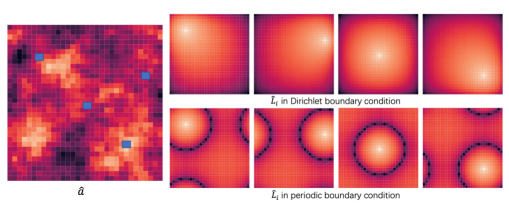
Figure 1: The diagram of Long range entanglements: taking Poisson’s equation as an example

3.3 LordNet

Although many modern neural network architectures have the capacity to model the long range entanglements, the de-facto architectures from other domains may not work well for solving PDEs, since the introduced inductive bias could be incompatible with various entanglements required by different PDEs. It is common that one neural network works well for a certain PDE, but works poorly for another, or even for the same one with a different boundary condition. For example, CNNs (LeCun et al., 1995) performs well in solving Poisson’s equation with the periodic boundary condition, while performs poorly in that with the Dirichlet boundary condition. This is because under the periodic boundary condition, collocation points at different places are identical and the assumption of the translation invariance naturally holds, as you can see from the second line of Fig. 1. However, such symmetry is broken under the Dirichlet boundary condition. Additionally, graph neural networks(GNNs) (Li et al., 2020c, b; Pfaff et al., 2020) have been introduced for solving PDEs recently. However, as Li et al. (2020a) pointed out, GNNs fail to converge in some important cases, such as turbulence modeling, because GNNs are originally designed for capturing local structures so that hard to support the long range entanglements. Transformer might be a possible choice since self-attention can resolve global entanglements and does not introduce too much inductive bias. However, the huge computational overhead of the global-wise attention for resolving global dependency will make neural networks less superior over the conventional numerical methods. In short, we need a lightweight network structure which can effectively resolves the long range entanglements and introduces little inductive bias at the same time.

To this end, we first use a multi-channel fully-connected layer to replace the expensive multi-head self-attention in Transformer block, since fully-connected layer is the most powerful but simple way to resolve linear global entanglements between input and output without any inductive bias. Specifically, a multi-channel fully-connected layer maps input $X\in\mathbb{R}^{C\times N}$ to output $Y\in\mathbb{R}^{C\times M}$ is defined as

$$Y_{c,m}=\sum_{n=1}^{N}W_{c,m,n}X_{c,n},$$ (8)

where $W\in\mathbb{R}^{C\times M\times N}$ is the weight tensor, $c=1,2,\cdots,C$, $n=1,2,\cdots,N$ and $m=1,2,\cdots,M$ are the indices of channel, input dimension and output dimension, respectively. Here, we linearly transform different channels independently, followed by a channel mixer without changing the dimensional of the channel. However, the weight matrix $W$ is unacceptable in practice since $N$ and $M$ are usually large for discretizing $\Omega$. Thus, we resort to a low-rank approximation to each channel of the weight matrix, that is,

$$W_{c}\simeq\sum_{r=1}^{R}\sigma_{c,r}a_{c,r}\otimes b_{c,r},$$ (9)

where $R$ is the rank of approximation, $\sigma_{r}$ are learnable singular values for $W_{c}$, $a_{c,r}\in\mathbb{R}^{M}$ and $b_{c,r}\in\mathbb{R}^{N}$ are corresponding left and right singular vectors, and $\otimes$ is the Kronecker product. In this way, we could diminish the parameter size from $CMN$ to $CR(M+N)$. We name the building block constructed this way as a Lord (Low-rank decomposition ) module, and a network consisting of Lord modules as LordNet. In practice, the input $\widehat{a}$ with $N$-point discretization is first lifted to a higher dimensional representation $\mathbb{R}^{C\times N}$ by a point-wise transformation, and then fed into the stacked Lord modules. The whole architecture of LordNet is illustrated in Fig. 2. Noted that $\ast W_{1\times 1}$ means the 1$\times$1 convolution and skip-connection here is different with the common used $(x+f(x))$, and we use $f_{1}(x)+f(x)$ as an alternative augmented shortcut, where $f_{1}$ is a 1$\times$1 convolution layer.

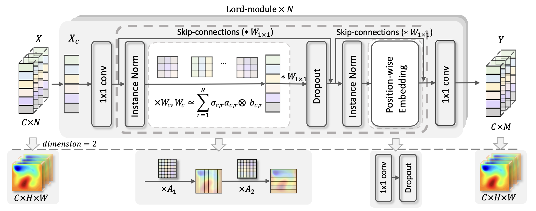
Figure 2: An illustration of LordNet architecture.

When the discretization of $\Omega\subseteq\mathbb{R}^{d}$ is uniform, the input matrix $X$ and output matrix $Y$ may be considered as high-dimensional tensors $\mathbb{R}^{C\times I_{1}\times\cdots\times I_{d}}$ and $\mathbb{R}^{C\times O_{1}\times\cdots\times O_{d}}$, respectively, where $I_{1}\times\cdots\times I_{d}=N$ and $O_{1}\times\cdots\times O_{d}=M$. This structure can be leveraged to further speed up the multi-channel fully-connected layer. Specifically, the rank-$R$ approximation of the weight tensor for each channel can be written as,

$$W_{c}\simeq\sum_{r=1}^{R}\sigma_{c,r}a_{c,r,1}\otimes b_{c,r,1}\otimes\cdots\otimes a_{c,r,d}\otimes b_{c,r,d},$$ (10)

where $a_{c,r,i}\in\mathbb{R}^{I_{i}}$ and $b_{c,r,i}\in\mathbb{R}^{O_{i}}$ for $i=1,\cdots,d$. In this way, the parameter size can be further reduced to $CR\sum_{i=1}^{d}(I_{i}+O_{i})$. However, we empirically find that the approximation in Eq. (10) usually need very large $R$ for good performance, since the parameters are too few to resolve the relation between inputs and outputs. Thus, we propose to approximate the weight tensor in a more representative way, that is,

$$W_{c}\simeq\sum_{r=1}^{R}\eta_{c,r}A_{c,r,1}\otimes A_{c,r,2}\otimes\dots\otimes A_{c,r,d},$$ (11)

where $A_{c,r,i}\in\mathbb{R}^{I_{i}\times O_{i}}$ for $i=1,2,\cdots,d$. Eq. (10) can be considered as a special case of Eq. (11) by letting $A_{c,r,i}$ be a rank-$1$ matrix with the decomposition $A_{c,r,i}=a_{c,r,i}\otimes b_{c,r,i}$, thus the learning capability of Eq. (11) is much better than that of Eq. (10), so that we can retain much fewer components to approximate $W$. In practice, $R=1$ is usually sufficient for good performance.

Further, it should be noted that the decomposition in Eq. (11) is not only a mathematical approximation, but also has a very clear physical meaning. We will discuss this with a 2-dimensional example, that is, $X\in\mathbb{R}^{C\times I_{1}\times I_{2}}$ and $Y\in\mathbb{R}^{C\times O_{1}\times O_{2}}$. In this case, the rank-$R$ approximation of the multi-channel linear transformation takes the form

$$Y_{c,o_{1},o_{2}}=\sum_{r=1}^{R}\sum_{i_{1}=1}^{I_{1}}\sum_{i_{2}=1}^{I_{2}}A_{c,r,i_{1},o_{1}}A_{c,r,i_{2},o_{2}}X_{c,i_{1},i_{2}},$$ (12)

which indicates that, for each channel and rank, the input matrix left multiplies a weight matrix and then right multiplies another weight matrix. The left multiplication first passes messages among positions row-wise, and then the right multiplication passes messages among positions column-wise, so that all positions could efficiently communicate with each other in this way.

We notice that the 2-dimensional version of LordNet shares similarities with several works in computer vision. For example, (Tolstikhin et al., 2021; Lee-Thorp et al., 2021) find that simple MLP performs comparable with CNNs and Transformer in computer vision and natural language processing tasks, respectively. The architectures they used can be seen as specific instances of LordNet, so we believe that, besides solving PDEs, LordNet might also perform well in traditional deep learning applications. We leave it for our future work.

Besides low-rank approximation to the fully-connected layer, Fourier transform is also an effective and efficient way to model the long range entanglements. For example, we empirically find that Fourier neural operator, which models the entanglements with Fast Fourier Transform (FFT), also performs well in multiple cases. However, FFT originally forms samples of a periodic spectrum and for problems with non-periodic boundary conditions, FNO has to add zero-paddings to correct the inductive bias. In addition, it ignores the high-frequency parts which may hurt the performance in some PDEs. As will be shown in our experiments, LordNet performs better than it in most of cases.

4 Experiments

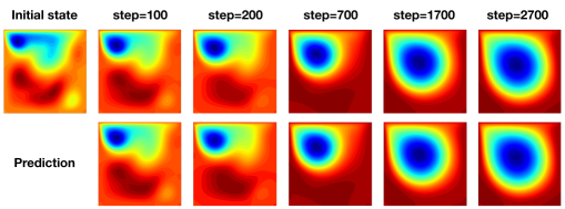
Figure 3: Solving Naiver-Stokes equation in lid-driven cavity with MSR loss and LordNet

In this section, we empirically demonstrate the advantages of the proposed MSR loss over the supervised MSE loss and showcase the LordNet’s capability to model the long range entanglements. We choose two representative and crucial PDEs, Poisson’s equation and Navier-Stokes equation, as the testbeds, which are notorious for difficult to solve efficiently.

Poisson’s Equation. 2-dimensional Poisson’s equation has been introduced in previous sections. We consider two boundary conditions, the Dirichlet boundary condition and the periodic boundary condition. The formula with the Dirichlet boundary condition is described in Eq. (3), which is used in our experiments. For the periodic boundary condition, the domain is cyclic at both dimensions.

Navier-Stokes Equation. We consider the 2-dimensional Naiver-Stokes equation in vorticity-stream function form as follows,

$$\frac{\partial\omega}{\partial t}=\frac{\partial\psi}{\partial y}\frac{\partial\omega}{\partial x}+\frac{\partial\psi}{\partial x}\frac{\partial\omega}{\partial y} +\frac{1}{\text{Re}}\left(\frac{\partial^{2}\omega}{\partial x^{2}}+\frac{\partial^{2}\omega}{\partial y^{2}}\right)$$ (13)

$$\frac{\partial^{2}\psi}{\partial x^{2}}+\frac{\partial^{2}\psi}{\partial y^{2}} =-\omega$$ (14)

where $\omega:[0,T]\times(0,1)^{2}\rightarrow\mathbb{R}$ is the vorticity function, $\psi:[0,T]\times(0,1)^{2}\rightarrow\mathbb{R}$ is the stream function, $\text{Re}\in\mathbb{R}_{+}$ is the Reynolds number. As a typical case of the time-dependent PDE, the neural network is used to predict the stream function in discrete timesteps in the auto-regressive manner. That is, the input of the neural network is the stream function at a certain timestep and the output is that of the next timestep. We consider the periodic boundary condition and Lid-driven cavity boundary condition. The periodic boundary condition sets the domain cyclic in both dimensions. In this case, $T$ is 2 seconds and the timestep is $1\mathrm{e}-2$ seconds. The Lid-driven cavity boundary condition (Zienkiewicz et al., 2006) is another well-known benchmark for viscous incompressible fluid flow, which is considered harder to solve than the periodic one. Specifically, the fluid acts in a cavity consisting of three rigid walls with no-slip conditions and a lid moving with a steady tangential velocity, which is set to 1 in our experiments. In this case, we evaluate for longer time, i.e., $T$ is 27 seconds with the timestep $1\mathrm{e}-2$ seconds. In both conditions, we set the viscosity $\nu=1\mathrm{e}-3$ and fix the resolution to 64$\times$64.

Neural network baselines. We choose the other three representative neural network architectures in our experiments. Resnet: Resnet (He et al., 2016) is famous and widely used in computer vision tasks. We use the residual blocks implemented in PyTorch and change the batch normalization to the layer normalization for better performance. Swin Transformer: Swin Transformer (Liu et al., 2021) leverages the Transformer architecture to handle computer vision tasks. It is popular and outperforms existing neural networks with a large gap in computer vision tasks. We directly use the implementation in its open-sourced project. FNO: Fourier neural operator is proposed in (Li et al., 2020a) that also solves parametric PDEs.

Numerical solvers and other configurations. We implement GPU-accelerated FDM solvers with the central differencing scheme for all cases as the numerical baselines, where the conjugate gradient method is used to solve the sparse linear algebraic equations. These numerical solvers are also used to collect training data and ground truth for test. In all experiments, we construct MSR loss functions with the same finite difference schemes as numerical solvers. Additionally, we trained all neural networks on a V100 GPU with Adam optimizer and decayed learning rates. The relative error is the evaluation metric for all experiments as the accuracy measurement, which is the Euclidean distance from the prediction to the ground truth divided by the Euclidean norm of the ground truth. For Navier-Stokes equation, we calculate two types of relative error, the one denoted as ‘Error-1’ is the one-step relative error and the other denoted as ‘Error-mul’ is the accumulated error of the terminal state when the model auto-regressively predicts along the timesteps.

4.1 Inductive biases for long range entanglements.

We first show how the inductive bias of a neural network influence the performance in PDEs with different physical entanglements. Following the discussion in Section 3.3, we use Poisson’s equation as the showcase and test the periodic boundary and the Dirichlet boundary with both CNN and LordNet. To model the long range entanglements, we construct the CNN by stacking multiple dilated convolutional layers to increase the receptive field to the whole domain. As is shown in Table 1, for the periodic boundary condition, both CNN and LordNet achieve a low relative error. However, for the Dirichlet boundary condition where the entanglements are not translation invariant, CNN works poorly. Because LordNet is flexible to model various long range entanglements, it performs well in both cases.

Table 1: Comparison on Poisson’s equation in terms of relative error and solution time (ms).

Boundary	Network	$n=32$		$n=128$
		Error	Time	Error	Time
Periodic	LordNet	0.0006	0.5	0.0021	1.2
Periodic	Conv	0.0008	0.8	0.0053	1.3
Dirichlet	LordNet	0.0531	0.5	0.0072	1.2
Dirichlet	Conv	0.7304	0.8	1.0343	1.3

4.2 Comparison on the LordNet

We conduct a more comprehensive study on the performance of different neural networks using Navier-Stokes equation with the Lid-driven cavity boundary condition. As we introduced previously, we believe that transformer, fourier transform and low-rank approximation are effective ways to model the long range entanglements. However, we find that Swin Transformer performs poorly in this setting. One possible reason is that the patch-wise self-attention is too coarse to model the ‘pixel-wise’ entanglements. The architecture based on the attention mechanism should be re-designed for the PDE solving tasks. FNO achieves relatively good results not only in this case, but also in the that with periodic boundary condition, as is shown in Table 2. However, FNO has to adjust the input and neural network structures for different boundary conditions, such as zero-padding for non-periodic boundary conditions. On the contrast, LordNet works well with no modification for arbitrary boundary conditions. In addition, FNO ignores the high-frequency parts, which we believe is the main reason why FNO is not as good as LordNet in the Lid-driven cavity case. Among all these neural networks, LordNet achieves the best result with the fewest parameters and the fastest inference speed. As Figure 3 shows, the simulation results by LordNet is nearly the same as the FDM solution and stabilizes to the same steady state as time goes. Compared to the GPU-accelerated FDM solution, LordNet has over 50 times speed-up.

4.3 Comparison on the MSR loss

Finally, we compare the proposed data-free paradigm to the data-driven approaches, which we choose the supervised MSE loss.

We first leverage the Navier-Stokes equation with the periodic boundary condition to compare the generalization ability of neural networks trained by two loss functions. To ensure the expressiveness of the neural network, we test with LordNet. For the MSE loss, we collect the training data by first sampling multiple initial conditions from a random distribution and then solving these PDEs with the FDM solver. We test the relative error on unseen initial conditions sampled from the same distribution within 2 seconds. To evaluate the generalization ability, we add the experiment where the simulation trajectories for training only covers the first 0.25 seconds. To be fair, the size of the training set is 6000 for both experiments. From the result in Table 2, we find that the performance drops obviously if we only provide the training data of the first 0.25 seconds. This indicates that the model trained with the MSE loss does not generalize well on the data at unseen timesteps. On the contrast, in the proposed data-free paradigm, we only use the distribution of the initial state. Therefore, we sample 6000 initial states as the training data for the MSR loss. The result shows that the model generalizes well over 2 seconds of simulation and even outperforms those trained with MSE loss.

Table 2: Comparison on Navier-Stokes equation with periodic boundary condition.

Method	Network	Parameters	$\nu=1\mathrm{e}-3,T=2$
			Error-1	Error-mul.
MSE (0~0.25s)	LordNet	1.15 M	0.0000235	0.00405
MSE (0~0.25s)	FNO	9.46 M	0.0001401	0.02265
MSE (0~2s)	LordNet	1.15 M	0.0000301	0.00232
MSE (0~2s)	FNO	9.46 M	0.0001278	0.01307
MSR (Initial only)	LordNet	1.15 M	0.0000107	0.00216
MSR (Initial only)	FNO	9.46 M	0.0000103	0.00213

Then we use the Lid-driven cavity boundary condition, a more challenging problem, to compare the performance of two loss functions. We test with other three representative neural network architectures, i.e., ResNet, Swin Transformer, and FNO. The simulation time is 27 seconds, which is 2700 timesteps in total. To prevent the generalization problem introduced above, the training data of the MSE loss cover the whole trajectories of 27 seconds, while for the MSR loss, we still only leverage the data of the initial conditions. As you can see from Table 3, there is an obvious performance gap between the neural networks trained with the MSE loss and those with the MSR loss, which indicates the effectiveness of the physical information in the MSR loss. In this case, the accumulation effect in the sequential prediction as long as 2700 timesteps requires the neural network to be very accurate at every timestep of the sequence. The accumulated relative error of both FNO and LordNet trained with the MSR loss is controled successfully under 5 percent, while all the other experiments fails even if the single-timestep relative error already reaches 0.1 percent or lower.

Table 3: Comparison on Naiver-Stokes equation with Lid-driven cavity boundary condition.

Method	Network	Error-1	Error-2700	Inference time(ms)	Parameter size
MSE	ResNet	0.001009	0.9589	5.131	1.21M
	Swin Transformer	0.000736	0.6731	23.011	59.82M
	FNO	0.000900	0.6950	1.659	9.46M
	LordNet	0.000631	0.4507	1.409	1.15M
MSR	ResNet	0.000561	0.4187	5.131	1.21M
	Swin Transformer	0.000282	0.7445	23.011	59.82M
	FNO	0.000045	0.0326	1.659	9.46M
	LordNet	0.000036	0.0172	1.409	1.15M

5 Discussion

Besides the MSR loss, there are some other lines of work in training neural network solver, as is introduced in section 2. In this section, we discuss two mainstream directions, the physics-informed loss and the data-driven approaches, on their pros and cons compared to the proposed method.

MSR versus PINN. This line of work, like DGM (Sirignano and Spiliopoulos, 2018) and PINN (Raissi et al., 2019), trained a network to approximate the solution function $u$ mapping from $\Omega$ to $\mathbb{R}$ given a specific $a$ rather than an operator mapping from $\mathcal{A}$ to $\mathcal{U}$. They can be seen as another way to learn from PDEs, where the derivatives of the function to be sought in the PDE are analytically replaced by the derivatives of the neural network. However, most of these works only solve specific PDEs. Although some works Wang et al. (2021) solve parametric PDEs, they still need supervised data. In addition, they have to introduce hyper-parameters to weigh the PDE loss, the boundary condition loss, the initial condition loss, and the data loss, which must be carefully tuned by experienced human experts because the network performance is very sensitive to them. In contrast, MSR loss is naturally constructed without any hyper-parameters since the algebraic operator $\widehat{\mathcal{L}}$ has already covered such information. Meanwhile, directly approximating the solution without discretization has the potential to prevent the curse of dimensionality, which is favourable in high-dimensional PDEs like Schrodinger equations.

Data-free versus data-driven. After discussing many advantages of MSR loss over previous data-driven methods, we would like to point out some disadvantages in this part. Our data-free method currently cannot resolve multi-scale features, i.e., predict high-resolution features on a low-resolution discretizaiton in either space or time, because the discretization used to construct MSR loss exactly determines what resolution the model could learn. However, some data-driven methods work well in this aspect. For example, Kochkov et al. (2021) resolved fine structure of forced turbulence on coarse mesh by learning correction and interpolation models from data, and Li et al. (2020a) learned a model from data to predict long-term behavior of forced turbulence so that achieve 3 orders of acceleration. Although both of them use periodic boundary and periodic external force field, making the problem relatively easy to deal with, their work still show potentials of data-driven methods in this aspect. We leave extending data-free method to this area for future work.

6 Conclusion

In this work, we introduced a data-free paradigm which directly constructs learning targets from PDEs. It doesn’t require any simulated data, so that makes deep learning-based PDE solver jump out of the chicken-egg dilemma. The experiments on solving Poisson’s equation and Navier-Stokes equation demonstrate that the proposed data-free paradigm outperforms previous data-driven methods in terms of both accuracy and generalization in PDE solving. Meanwhile, the proposed LordNet, which efficiently builds long range entanglements, outperforms modern neural network architectures including the SOTA neural operatorLi et al. (2020a).

References

- Bar-Sinai et al. [2019] Yohai Bar-Sinai, Stephan Hoyer, Jason Hickey, and Michael P Brenner. Learning data-driven discretizations for partial differential equations. Proceedings of the National Academy of Sciences, 116(31):15344–15349, 2019.
- Berner et al. [2020] Julius Berner, Markus Dablander, and Philipp Grohs. Numerically solving parametric families of high-dimensional kolmogorov partial differential equations via deep learning. arXiv preprint arXiv:2011.04602, 2020.
- Bhatnagar et al. [2019] Saakaar Bhatnagar, Yaser Afshar, Shaowu Pan, Karthik Duraisamy, and Shailendra Kaushik. Prediction of aerodynamic flow fields using convolutional neural networks. Computational Mechanics, 64(2):525–545, 2019.
- Brandstetter et al. [2022] Johannes Brandstetter, Daniel Worrall, and Max Welling. Message passing neural pde solvers. arXiv preprint arXiv:2202.03376, 2022.
- Geneva and Zabaras [2020] Nicholas Geneva and Nicholas Zabaras. Modeling the dynamics of pde systems with physics-constrained deep auto-regressive networks. Journal of Computational Physics, 403:109056, 2 2020. ISSN 00219991. doi: 10.1016/j.jcp.2019.109056. URL https://linkinghub.elsevier.com/retrieve/pii/S0021999119307612.
- Guo et al. [2016] Xiaoxiao Guo, Wei Li, and Francesco Iorio. Convolutional neural networks for steady flow approximation. Proceedings of the 22nd ACM SIGKDD international conference on knowledge discovery and data mining, pages 481–490, 2016.
- Han et al. [2018] Jiequn Han, Arnulf Jentzen, and E Weinan. Solving high-dimensional partial differential equations using deep learning. Proceedings of the National Academy of Sciences, 115(34):8505–8510, 2018.
- Harlow and Welch [1965] Francis H Harlow and J Eddie Welch. Numerical calculation of time-dependent viscous incompressible flow of fluid with free surface. The physics of fluids, 8(12):2182–2189, 1965.
- He et al. [2016] Kaiming He, Xiangyu Zhang, Shaoqing Ren, and Jian Sun. Deep residual learning for image recognition. In Proceedings of the IEEE conference on computer vision and pattern recognition, pages 770–778, 2016.
- Hermann et al. [2020] Jan Hermann, Zeno Schätzle, and Frank Noé. Deep-neural-network solution of the electronic schrödinger equation. Nature Chemistry, 12(10):891–897, 2020.
- Hsieh et al. [2019] Jun-Ting Hsieh, Shengjia Zhao, Stephan Eismann, Lucia Mirabella, and Stefano Ermon. Learning neural pde solvers with convergence guarantees. In International Conference on Learning Representations, 2019.
- Jin et al. [2021] Xiaowei Jin, Shengze Cai, Hui Li, and George Em Karniadakis. Nsfnets (navier-stokes flow nets): Physics-informed neural networks for the incompressible navier-stokes equations. Journal of Computational Physics, 426:109951, 2021.
- Knoll and Keyes [2004] Dana A Knoll and David E Keyes. Jacobian-free newton–krylov methods: a survey of approaches and applications. Journal of Computational Physics, 193(2):357–397, 2004.
- Kochkov et al. [2021] Dmitrii Kochkov, Jamie A Smith, Ayya Alieva, Qing Wang, Michael P Brenner, and Stephan Hoyer. Machine learning accelerated computational fluid dynamics. arXiv preprint arXiv:2102.01010, 2021.
- Landau and Lifshitz [2013] Lev Davidovich Landau and Evgenii Mikhailovich Lifshitz. Course of theoretical physics. Elsevier, 2013.
- LeCun et al. [1995] Yann LeCun, Yoshua Bengio, et al. Convolutional networks for images, speech, and time series. The handbook of brain theory and neural networks, 3361(10):1995, 1995.
- Lee-Thorp et al. [2021] James Lee-Thorp, Joshua Ainslie, Ilya Eckstein, and Santiago Ontanon. Fnet: Mixing tokens with fourier transforms. arXiv preprint arXiv:2105.03824, 2021.
- Li et al. [2020a] Zongyi Li, Nikola Kovachki, Kamyar Azizzadenesheli, Burigede Liu, Kaushik Bhattacharya, Andrew Stuart, and Anima Anandkumar. Fourier neural operator for parametric partial differential equations. arXiv preprint arXiv:2010.08895, 2020a.
- Li et al. [2020b] Zongyi Li, Nikola Kovachki, Kamyar Azizzadenesheli, Burigede Liu, Kaushik Bhattacharya, Andrew Stuart, and Anima Anandkumar. Neural operator: Graph kernel network for partial differential equations. arXiv preprint arXiv:2003.03485, 2020b.
- Li et al. [2020c] Zongyi Li, Nikola Kovachki, Kamyar Azizzadenesheli, Burigede Liu, Andrew Stuart, Kaushik Bhattacharya, and Anima Anandkumar. Multipole graph neural operator for parametric partial differential equations. In Advances in Neural Information Processing Systems, volume 33, pages 6755–6766, 2020c.
- Ling et al. [2016] Julia Ling, Andrew Kurzawski, and Jeremy Templeton. Reynolds averaged turbulence modelling using deep neural networks with embedded invariance. Journal of Fluid Mechanics, 807:155–166, 2016.
- Liu et al. [2021] Ze Liu, Yutong Lin, Yue Cao, Han Hu, Yixuan Wei, Zheng Zhang, Stephen Lin, and Baining Guo. Swin transformer: Hierarchical vision transformer using shifted windows. arXiv preprint arXiv:2103.14030, 2021.
- Lu et al. [2021] Lu Lu, Pengzhan Jin, Guofei Pang, Zhongqiang Zhang, and George Em Karniadakis. Learning nonlinear operators via deeponet based on the universal approximation theorem of operators. Nature Machine Intelligence, 3(3):218–229, 2021.
- Pfaff et al. [2020] Tobias Pfaff, Meire Fortunato, Alvaro Sanchez-Gonzalez, and Peter W Battaglia. Learning mesh-based simulation with graph networks. arXiv preprint arXiv:2010.03409, 2020.
- Pfau et al. [2020] David Pfau, James S Spencer, Alexander GDG Matthews, and W Matthew C Foulkes. Ab initio solution of the many-electron schrödinger equation with deep neural networks. Physical Review Research, 2(3):033429, 2020.
- Raissi et al. [2019] Maziar Raissi, Paris Perdikaris, and George E Karniadakis. Physics-informed neural networks: A deep learning framework for solving forward and inverse problems involving nonlinear partial differential equations. Journal of Computational Physics, 378:686–707, 2019.
- Raissi et al. [2020] Maziar Raissi, Alireza Yazdani, and George Em Karniadakis. Hidden fluid mechanics: Learning velocity and pressure fields from flow visualizations. Science, 367(6481):1026–1030, 2020.
- Saad [2003] Yousef Saad. Iterative methods for sparse linear systems. Society for Industrial and Applied Mathematics, 2003.
- Sirignano and Spiliopoulos [2018] Justin Sirignano and Konstantinos Spiliopoulos. Dgm: A deep learning algorithm for solving partial differential equations. Journal of computational physics, 375:1339–1364, 2018.
- Tolstikhin et al. [2021] Ilya Tolstikhin, Neil Houlsby, Alexander Kolesnikov, Lucas Beyer, Xiaohua Zhai, Thomas Unterthiner, Jessica Yung, Daniel Keysers, Jakob Uszkoreit, Mario Lucic, et al. Mlp-mixer: An all-mlp architecture for vision. arXiv preprint arXiv:2105.01601, 2021.
- Um et al. [2020] Kiwon Um, Robert Brand, Yun (Raymond) Fei, Philipp Holl, and Nils Thuerey. Solver-in-the-loop: Learning from differentiable physics to interact with iterative pde-solvers. In Advances in Neural Information Processing Systems, volume 33, pages 6111–6122, 2020.
- Wandel et al. [2020] Nils Wandel, Michael Weinmann, and Reinhard Klein. Learning Incompressible Fluid Dynamics from Scratch – Towards Fast, Differentiable Fluid Models that Generalize. arXiv preprint, 2020. URL http://arxiv.org/abs/2006.08762.
- Wandel et al. [2021] Nils Wandel, Michael Weinmann, Michael Neidlin, and Reinhard Klein. Spline-PINN: Approaching PDEs without Data using Fast, Physics-Informed Hermite-Spline CNNs. arXiv preprint, 2021. URL http://arxiv.org/abs/2109.07143.
- Wang et al. [2021] Sifan Wang, Hanwen Wang, and Paris Perdikaris. Learning the solution operator of parametric partial differential equations with physics-informed deeponets. arXiv preprint arXiv:2103.10974, 2021.
- Zhu and Zabaras [2018] Yinhao Zhu and Nicholas Zabaras. Bayesian deep convolutional encoder–decoder networks for surrogate modeling and uncertainty quantification. Journal of Computational Physics, 366:415–447, 2018.
- Zienkiewicz et al. [2006] O.C. Zienkiewicz, R.L. Taylor, and P. Nithiarasu. The finite element method for fluid dynamics. 6th edition. Elsevier, 2006.