The Frenet Frame as a Generalization
of the Park Transform

Abstract

The paper proposes a generalization of the Park transform based on the Frenet frame, which is a special set of coordinates defined in differential geometry for space curves. The proposed geometric transform is first discussed for three dimensions, which correspond to the common three-phase circuits. Then, the expression of the time derivative of the proposed transform is discussed and the Frenet-Serret formulas and the Darboux vector are introduced. The change of reference frame and its differentiation based on Cartan’s moving frames and attitude matrices are also described. Finally, the extension to circuits with more than three phases is presented. The features of the Frenet frame are illustrated through a variety of examples, including a case study based on the IEEE 39-bus system.

I Notation

Scalars are indicated with Italic font, e.g. $x$, whereas vectors and matrices are indicated in bold face, e.g. $\boldsymbol{x}=(x_{1},x_{2},x_{3})$. Vectors have order 3, unless otherwise indicated.

Scalars

• length of a curve

• time

• voltage magnitude

• $2\pi/3$ rad

• $2\pi/6$ rad

• synchronous machine rotor angle

• voltage phase angle

• curvature

• projection operator

• torsion

• generalized curvature

• angular frequency

Vectors

• null vector

• binormal vector of the Frenet frame

• $i$-th vector of an orthonormal basis

• $i$-th vector of a generalized Frenet frame

• current vector

• normal vector of the Frenet frame

• Darboux angular momentum vector

• tangent vector of the Frenet frame

• voltage vector

• magnetic flux vector

Matrices

• attitude matrix of Cartan’s moving frame

• cylindrical frame

• matrix of the Frenet frame

• matrix of the Park transform

• generalized matrix to change coordinates

• rotation matrix

Vector and Matrix Operations

• vector magnitude

• derivative of a scalar/vector/matrix w.r.t. $t$

• derivative of a scalar/vector/matrix w.r.t. $s$

• transpose of a vector/matrix

• inverse of a matrix

II Introduction

II-A Motivation

The Park transform is the most important transform utilized in power system transient stability analysis and control. Originally formulated by Park for the two-reaction theory of synchronous machines [1], this transform has found applications in the control of induction machines and, more recently, of converter-interfaced devices. In simulations, the Park transform is also a fundamental tool for the implementation of the devices that compose the grid [2] and for the modeling on power electronic converters [3]. Despite its relevance, there are not many attempts to generalize the Park transform, except for some extensions to multi-phase circuits [4, 5], nor to overcome its intrinsic idiosyncrasies or better understand its geometric properties. This work addresses precisely these issues through the theory provided by differential geometry.

II-B Literature Review

Since the introduction of phasors by Steinmetz at the end of the 19th century [6], domain and coordinate transformations are a common practice for the analysis of electrical circuits, electrical machines and for power system modeling, analysis and control. Apart from the aforementioned Park transform, well-known transforms are the harmonic analysis through Fourier series [7], Fortescue symmetrical component theory [8], the forward-backward transform [9], the Clarke transform [10], and more recently, dynamic phasor analysis [11, 12]. Except for the Fourier analysis, the transforms above can be represented as 3-by-3 matrices when applied to three-phase circuits. Begin homomorphisms, it is also possible to find the conversion matrices from one transform to another (see, e.g., [13]). In the same vein, this work aims at discussing a generalization of the concept of change of coordinates and considers the most general case, i.e., the case for which the axis of the coordinates are time dependent.

The proposed generalization is inspired by the literature on differential geometry and, in particular, by the Frenet frame, the Frenet-Serret formulas and the theory of moving frames developed by Cartan [14, 15]. These have found several applications in mechanics, e.g., just to cite a recent relevant one, in the area of autonomous vehicle driving [16, 17]. On the other hand, the Frenet frame has been only very recently considered for circuit and power systems analysis [18]. This was given raise by the geometrical interpretation of the frequency developed by the author in [19].

References [18] and [19] assume that the instantaneous values of electrical quantities such as voltages and currents of three- or multi-phase circuits are vectors in a given coordinate system. This idea was already developed in the past in the context of the instantaneous power theory [20, 21, 22, 23]. These works define the active and reactive power as the dot and cross (or wedge in multi-phase circuits) products, respectively, of voltage and currents. A variety of recent works with same starting point have focused on the analysis of electric circuits using the formalism provided by geometric algebra [24, 25, 26, 27].

The main difference of [18] and [19] with respect to the more conventional theory on instantaneous power is the hypothesis that the voltage (current) vector is the speed of a curve, represented by the magnetic flux (electric charge). This interpretation moves the focus from “algebra” to “calculus” and allows interpreting the dynamic behavior of the voltage and current in terms of the “invariants” of differential geometry, such as curve length, curvature and torsion.

II-C Contributions

This work elaborates on the results of [18] and determines similarities and differences between the Park transform and the Frenet frame. The novel contributions are the following.

• The derivation of the formal conditions under which the Park transform and its time derivative is equivalent to the Frenet frame and to the Frenet-Serret formulas.

• An application of Cartan’s moving frames that allows interfacing the local Frenet frame of each device connected to the grid to the reference frame of the grid itself.

• An application of generalized $n$-dimensional Frenet frame to multi-phase systems, i.e., systems with more than three phases.

• A thorough example-based discussion of the added value of the Frenet frame compared to the Park transform for the study of the dynamic performance of power systems.

II-D Organization

The remainder of the paper is organized as follows. Section III recalls the definition of the Park transform and its time derivative. Section IV introduces geometric calculus, provides the definitions of curve length, curvature and torsion, recalls the Frenet frame, the Frenet-Serret formulas and Cartan’s moving frames and provides the formulas of the generalized curvatures in $n$ dimensions. Section V combines the definitions provided in the previous sections and defines the conditions under which the Park transform is a special case of the Frenet frame. The interconnection of local Frenet frames of electrical devices with the reference frame of the grid is also discussed in Section V by means of Cartan’s moving frames. Section VI illustrates the differences between the Park transform and the Frenet frame through a series of examples in three and six dimensions as well as the IEEE 39-bus system. Section VII draws conclusions and outlines future work.

III Park Transform

The Park transform projects the phase components $abc$ of a three-phase electrical quantity onto a $dqo$ frame, where the axes $d$ and $q$ rotate at angular speed $\omega_{\scriptscriptstyle\rm P}$. In his original formulation, Park aimed at preserving the magnitudes of the transformed quantities and did not define a power invariant transformation. For the developments presented in this paper, however, it is more convenient to retain power invariance.

The formulation of the $dqo$-transform utilized in this paper is as follows:

$$\boldsymbol{v}_{dqo}(t)=\boldsymbol{\rm P}(\omega_{\scriptscriptstyle\rm P})\,\boldsymbol{v}_{abc}(t)\,,$$ (1)

where $\hat{\boldsymbol{v}}_{dqo}=[v_{d},v_{q},v_{o}]$, $\hat{\boldsymbol{v}}_{abc}=[v_{a},v_{b},v_{c}]$, and

$$\boldsymbol{\rm P}(\omega_{\scriptscriptstyle\rm P})=\sqrt{\frac{2}{3}}\begin{bmatrix}\sin(\theta_{\scriptscriptstyle\rm P})&\sin(\theta_{\scriptscriptstyle\rm P}-\alpha)&\sin(\theta_{\scriptscriptstyle\rm P}+\alpha)\\ \cos(\theta_{\scriptscriptstyle\rm P})&\cos(\theta_{\scriptscriptstyle\rm P}-\alpha)&\cos(\theta_{\scriptscriptstyle\rm P}+\alpha)\\ \nicefrac{{1}}{{\sqrt{2}}}&\nicefrac{{1}}{{\sqrt{2}}}&\nicefrac{{1}}{{\sqrt{2}}}\end{bmatrix}\normalsize,$$ (2)

where:

$$\theta_{\scriptscriptstyle\rm P}(t) =\int_{0}^{t}\omega_{\scriptscriptstyle\rm P}(r)\,dr+\theta_{{\scriptscriptstyle\rm P},0}\,.$$ (3)

Note that $\omega_{\scriptscriptstyle\rm P}$ in (3) does not have to be constant. The power invariance of the matrix $\boldsymbol{\rm P}$ in (2) refers to the fact that if $\boldsymbol{v}_{abc}$ and $\boldsymbol{\imath}_{abc}$ are the voltage and current at a given point of a three-phase circuits, then the instantaneous power is unchanged for the same voltage and current transformed in $dqo$ coordinates:

$$\hat{\boldsymbol{v}}_{abc}(t)\,\boldsymbol{\imath}_{abc}(t)=\hat{\boldsymbol{v}}_{dqo}(t)\,\boldsymbol{\imath}_{dqo}(t)\,,$$ (4)

This property descends from the fact that $\boldsymbol{\rm P}$ is orthonormal, i.e., its transpose is equal to its inverse:

$$\hat{\boldsymbol{\rm P}}(\omega_{\scriptscriptstyle\rm P})=\bar{\boldsymbol{\rm P}}(\omega_{\scriptscriptstyle\rm P})\,.$$ (5)

Equation (5) can be readily proved, as follows:

$$\hat{\boldsymbol{v}}_{dqo}\boldsymbol{\imath}_{dqo} =\widehat{(\boldsymbol{\rm P}\,\boldsymbol{v}_{abc})}\boldsymbol{\rm P}\,\boldsymbol{\imath}_{abc}$$

$$=\hat{\boldsymbol{v}}_{abc}\,\hat{\boldsymbol{\rm P}}\boldsymbol{\rm P}\,\boldsymbol{\imath}_{abc}$$

$$=\hat{\boldsymbol{v}}_{abc}\,\bar{\boldsymbol{\rm P}}\boldsymbol{\rm P}\,\boldsymbol{\imath}_{abc}=\hat{\boldsymbol{v}}_{abc}\boldsymbol{\imath}_{abc}\,,$$

where the dependencies on time and on $\omega_{\scriptscriptstyle\rm P}$ have been dropped for simplicity.

The choice for the angular speed $\omega_{\scriptscriptstyle\rm P}$ of the Park transform depends on the device and the application. For synchronous machines, $\omega_{\scriptscriptstyle\rm P}$ is generally chosen as the rotor angular speed of the machine itself, namely $\omega_{\scriptscriptstyle\rm P}=\omega_{r}=\delta_{r}^{\prime}$. This allows simplifying the equations of the machine and rewriting rotor quantities and equations as they were a dc circuit. This is also the motivation for the original two-reaction theory developed by Park. For all other devices, however, including induction machines, and in general for transient stability analysis studies of interconnected systems, it is chosen $\omega_{\scriptscriptstyle\rm P}=\omega_{o}$, namely, the constant synchronous reference angular frequency of the grid, e.g., $\omega_{o}=2\pi\,60$ rad/s.

III-A Time Derivative of $dqo$-Axis Voltages

The time derivative of a $dqo$-axis voltage is given by:

$$\boldsymbol{v}^{\prime}_{dqo} =\big{(}\boldsymbol{\rm P}\,\boldsymbol{v}_{abc}\big{)}^{\prime}$$ (6)

$$=\boldsymbol{\rm P}^{\prime}\boldsymbol{v}_{abc}+\boldsymbol{\rm P}\,\boldsymbol{v}^{\prime}_{abc}$$

$$=\boldsymbol{\rm P}^{\prime}\,\bar{\boldsymbol{\rm P}}\boldsymbol{v}_{dqo}+\boldsymbol{\rm P}\,\boldsymbol{v}^{\prime}_{abc}\,,$$

where the dependency of $\boldsymbol{\rm P}$ on $\omega_{\scriptscriptstyle\rm P}$ has been dropped for simplicity. Let us define:

$$\boldsymbol{\rm\Omega}_{\scriptscriptstyle\rm P}=\boldsymbol{\rm P}^{\prime}\,\bar{\boldsymbol{\rm P}}=\boldsymbol{\rm P}^{\prime}\,\hat{\boldsymbol{\rm P}}=\begin{bmatrix}0&\omega_{\scriptscriptstyle\rm P}&0\\ -\omega_{\scriptscriptstyle\rm P}&0&0\\ 0&0&0\end{bmatrix},$$ (7)

which is a skew-symmetric matrix, i.e., $\hat{\boldsymbol{\rm\Omega}}_{\scriptscriptstyle\rm P}=-\boldsymbol{\rm\Omega}_{\scriptscriptstyle\rm P}$. Then, (6) can be rewritten as:

$$\boldsymbol{\rm P}\,\boldsymbol{v}^{\prime}_{abc} =\boldsymbol{v}^{\prime}_{dqo}-\boldsymbol{\rm\Omega}_{\scriptscriptstyle\rm P}\,\boldsymbol{v}_{dqo}$$ (8)

$$=\boldsymbol{v}^{\prime}_{dqo}+\hat{\boldsymbol{\rm\Omega}}_{\scriptscriptstyle\rm P}\,\boldsymbol{v}_{dqo}\,.$$

Equation (8) shows that the Park transform of the derivative of $\boldsymbol{v}_{abc}$ consists of two terms. The first term is the time derivative of the Park-transformed voltage $\boldsymbol{v}_{dqo}$, which represents a translation. The second term is given by product of $\boldsymbol{\rm\Omega}_{\scriptscriptstyle\rm P}$ and $\boldsymbol{v}_{dqo}$, which is due to the rotation of the Park $dq$-axis. The second term is null only if $\omega_{\scriptscriptstyle\rm P}=0$, which is the choice that leads to the Clarke transform.

III-B Interface between $dqo$-Axes Rotating at Different Speeds

We consider the relevant case of the interface of the stator terminal-bus synchronous generator with Park transform $\boldsymbol{\rm P}(\omega_{r})$ with the grid, the Park transform of which is $\boldsymbol{\rm P}(\omega_{s})$. Since the zero-axis of the Park transform does not rotate with $\omega_{\scriptscriptstyle\rm P}$, the interface between machine and network consists in a rotation in the $dq$-plane, as follows:

$$\boldsymbol{v}_{dqo}^{N}(t) =\boldsymbol{\rm P}(\omega_{s})\,\boldsymbol{v}_{abc}(t)$$ (9)

$$=\boldsymbol{\rm P}(\omega_{s})\,\hat{\boldsymbol{\rm P}}(\omega_{r})\,\boldsymbol{v}_{dqo}^{G}(t)$$

$$=\boldsymbol{\rm C}\,\boldsymbol{v}_{dqo}^{G}(t)\,,$$

where $N$ and $G$ indicate “network” and “generator”, respectively, and matrix $\boldsymbol{\rm C}$ is orthonormal and represents a change of coordinates in a cylindrical frame. In fact, developing the matrix multiplication between $\boldsymbol{\rm P}(\omega_{s})$ and $\hat{\boldsymbol{\rm P}}(\omega_{r})$, one obtains:

$$\boldsymbol{\rm C}=\begin{bmatrix}\cos(\theta_{s}-\delta_{r})&-\sin(\theta_{s}-\delta_{r})&0\\ \sin(\theta_{s}-\delta_{r})&\cos(\theta_{s}-\delta_{r})&0\\ 0&0&1\\ \end{bmatrix},$$ (10)

where $\delta_{r}=\int_{0}^{t}\omega_{r}(r)-\omega_{o}\,dr+\delta_{r,0}$ is the rotor angular position of the machine and $\theta_{s}=\int_{0}^{t}\omega_{s}(r)-\omega_{o}\,dr+\theta_{s,0}$ is the phase angle of the terminal-bus voltage of the machine. In practical implementations, one can only know a relative value of the phase angles. For this reason $\delta_{r}$ and $\theta_{s}$ must be referred to the same reference frame, which is generally chosen as rotating at the constant reference angular speed $\omega_{o}$. Another common choice for the reference is the angular frequency of the center of inertia of the system [2]. This is utilized to avoid the drift of the machine angles and bus voltage phase angles during the transients following a large perturbation [28].

Finally, the time derivative at the interface between a generator and the network can be obtained in a similar way as described in the previous section, as follows:

$$(\boldsymbol{v}_{dqo}^{N})^{\prime} =\big{(}\boldsymbol{\rm P}(\omega_{s})\,\boldsymbol{v}_{abc}\big{)}^{\prime}$$ (11)

$$=\boldsymbol{\rm P}^{\prime}(\omega_{s})\boldsymbol{v}_{abc}+\boldsymbol{\rm P}(\omega_{s})\,\boldsymbol{v}_{abc}^{\prime}$$

$$=\boldsymbol{\rm P}^{\prime}(\omega_{s})\,\hat{\boldsymbol{\rm P}}(\omega_{r})\boldsymbol{v}_{dqo}^{G}+\boldsymbol{\rm P}(\omega_{s})\,\boldsymbol{v}_{abc}^{\prime}\,,$$

and substituting

$$\boldsymbol{v}_{abc}^{\prime}=\hat{\boldsymbol{\rm P}}(\omega_{r})(\boldsymbol{v}_{dqo}^{G})^{\prime}-\hat{\boldsymbol{\rm P}}(\omega_{r})\boldsymbol{\rm\Omega}_{\scriptscriptstyle\rm P}(\omega_{r})\boldsymbol{v}_{dqo}^{G}\,,$$ (12)

one obtains:

$$(\boldsymbol{v}_{dqo}^{N})^{\prime} =\boldsymbol{\rm C}\,(\boldsymbol{v}_{dqo}^{G})^{\prime}$$ (13)

$$+[\boldsymbol{\rm P}^{\prime}(\omega_{s})\,\hat{\boldsymbol{\rm P}}(\omega_{r})-\boldsymbol{\rm C}\,\boldsymbol{\rm\Omega}_{\scriptscriptstyle\rm P}(\omega_{r})]\boldsymbol{v}_{dqo}^{G}\,.$$

Observing that:

$$\boldsymbol{\rm P}^{\prime}(\omega_{s})\,\hat{\boldsymbol{\rm P}}(\omega_{r}) =\boldsymbol{\rm P}^{\prime}(\omega_{s})\,\hat{\boldsymbol{\rm P}}(\omega_{s})\,\boldsymbol{\rm P}(\omega_{s})\,\hat{\boldsymbol{\rm P}}(\omega_{r})$$ (14)

$$=\boldsymbol{\rm\Omega}_{\scriptscriptstyle\rm P}(\omega_{s})\,\boldsymbol{\rm C}\,,$$

and that $\boldsymbol{\rm\Omega}_{\scriptscriptstyle\rm P}(\omega_{s})\,\boldsymbol{\rm C}=\boldsymbol{\rm C}\,\boldsymbol{\rm\Omega}_{\scriptscriptstyle\rm P}(\omega_{s})$, one obtains:

$$(\boldsymbol{v}_{dqo}^{N})^{\prime} =\boldsymbol{\rm C}\,(\boldsymbol{v}_{dqo}^{G})^{\prime}$$ (15)

$$+\boldsymbol{\rm C}\,[\boldsymbol{\rm\Omega}_{\scriptscriptstyle\rm P}(\omega_{s})-\boldsymbol{\rm\Omega}_{\scriptscriptstyle\rm P}(\omega_{r})]\boldsymbol{v}_{dqo}^{G}\,,$$

where it is relevant to observe that the term $\boldsymbol{\rm\Omega}_{\scriptscriptstyle\rm P}(\omega_{s})-\boldsymbol{\rm\Omega}_{\scriptscriptstyle\rm P}(\omega_{r})$ can be also obtained as:

$$\boldsymbol{\rm C}^{\prime}\,\hat{\boldsymbol{\rm C}}=\begin{bmatrix}0&\omega_{s}-\omega_{r}&0\\ \omega_{r}-\omega_{s}&0&0\\ 0&0&0\end{bmatrix}.$$ (16)

The latter expression does not appear out of the blue. It is the consequence of a more general theory, i.e., Cartan’s moving frames, which is described in the next section.

IV Frenet Frame of Space Curves

This section introduces the classical Frenet frame and the Frenet-Serret formulas of space curves. With this aim, it is relevant to provide first some definitions.

The starting point is a curve in a three-dimensional space, say $\boldsymbol{x}=(x_{1},x_{2},x_{3})$ or, equivalently:

$$\boldsymbol{x}=x_{1}\,\boldsymbol{\rm e}_{\rm 1}+x_{2}\,\boldsymbol{\rm e}_{\rm 2}+x_{3}\,\boldsymbol{\rm e}_{\rm 3}\,,$$ (17)

where $(\boldsymbol{\rm e}_{\rm 1},\boldsymbol{\rm e}_{\rm 2},\boldsymbol{\rm e}_{\rm 3})$ is an orthonormal basis. For the development given below, it is relevant to define two types of products that can be done with three-dimensional vectors, namely the dot product and and the cross product. The dot product of two vectors returns a scalar, as follows:

$$\boldsymbol{x}\cdot\boldsymbol{y}=\hat{\boldsymbol{x}}\,\boldsymbol{y}=x_{1}y_{1}+x_{2}y_{2}+x_{3}y_{3}\,.$$ (18)

The cross product of two vectors returns a vector that is orthogonal to the original vectors, as follows:

$$\boldsymbol{x}\times\boldsymbol{y} =\left|\begin{matrix}\boldsymbol{\rm e}_{\rm 1}&\boldsymbol{\rm e}_{\rm 2}&\boldsymbol{\rm e}_{\rm 3}\\ x_{1}&x_{2}&x_{3}\\ y_{1}&y_{2}&y_{3}\\ \end{matrix}\right|\,.$$ (19)

It is relevant to note that ${|\boldsymbol{x}|}=\sqrt{\boldsymbol{x}\cdot\boldsymbol{x}}$ is the magnitude of the vector, and $\boldsymbol{x}\times\boldsymbol{x}=\boldsymbol{0}$.

The length $s$ of the curve is defined as:

$$s=\int_{0}^{t}\sqrt{(\boldsymbol{x}^{\prime}\cdot\boldsymbol{x}^{\prime})}\,dt\,,$$ (20)

or, equivalently:

$$s^{\prime}=\sqrt{\boldsymbol{x}^{\prime}\cdot\boldsymbol{x}^{\prime}}=|\boldsymbol{x}^{\prime}|\,.$$ (21)

where

$$\boldsymbol{x}^{\prime}= \;(x_{1}\,\boldsymbol{\rm e}_{\rm 1})^{\prime}+(x_{2}\,\boldsymbol{\rm e}_{\rm 2})^{\prime}+(x_{3}\,\boldsymbol{\rm e}_{\rm 3})^{\prime}$$ (22)

$$= \;(x^{\prime}_{1}\,\boldsymbol{\rm e}_{\rm 1}+x^{\prime}_{2}\,\boldsymbol{\rm e}_{\rm 2}+x^{\prime}_{3}\,\boldsymbol{\rm e}_{\rm 3})+$$

$$\;(x_{1}\,\boldsymbol{\rm e}_{\rm 1}^{\prime}+x_{2}\,\boldsymbol{\rm e}_{\rm 2}^{\prime}+x_{3}\,\boldsymbol{\rm e}_{\rm 3}^{\prime})$$

is the speed of the trajectory described by $\boldsymbol{x}$. For fixed reference frames the terms $\boldsymbol{\rm e}_{\rm i}^{\prime}$ are null. However, in this work, it is of interest to discuss moving frames, i.e., sets of coordinates for which the position of the axes of the coordinates vary in time. Both the Park transform and the Frenet frame, which are introduced below, are special cases of moving frames.

The length $s$ is a geometric invariant, i.e., its value does not depend on the choice of the coordinates. Neglecting relativistic effects, also its time derivative, $s^{\prime}$, is an invariant and has a special role in differential geometry. In particular, it is relevant to define The derivative of $\boldsymbol{x}$ with respect to $s$, which, using the chain rule, can be written as:

$$\dot{\boldsymbol{x}}=\frac{d\boldsymbol{x}}{ds}=\frac{d\boldsymbol{x}}{dt}\frac{dt}{ds}=\frac{\boldsymbol{x}^{\prime}}{s^{\prime}}=\frac{\boldsymbol{x}^{\prime}}{|\boldsymbol{x}^{\prime}|}\,.$$ (23)

The vector $\dot{\boldsymbol{x}}$ has magnitude 1 and is tangent to the curve $\boldsymbol{x}$. In the remainder of this paper, $\dot{\boldsymbol{x}}$, $\ddot{\boldsymbol{x}}$, $\dddot{\boldsymbol{x}}$, etc. indicate the derivatives of a vector with respect to $s$, whereas $\boldsymbol{x}^{\prime}$, $\boldsymbol{x}^{\prime\prime}$, $\boldsymbol{x}^{\prime\prime\prime}$ indicate time derivatives.

We have mentioned that invariants play a relevant role in differential geometry as they are quantities independent form the choice of the coordinates. Yet, among all possible set of coordinates, there is one, the Frenet frame, that has special properties. This frame is defined by the following three vectors:

$${\scriptstyle\rm\boldsymbol{\rm T}}=\dot{\boldsymbol{x}}\,,\qquad {\scriptstyle\rm\boldsymbol{\rm N}}=\frac{\ddot{\boldsymbol{x}}}{|\ddot{\boldsymbol{x}}|}\,, {\scriptstyle\rm\boldsymbol{\rm B}}={\scriptstyle\rm\boldsymbol{\rm T}}\times{\scriptstyle\rm\boldsymbol{\rm N}}\,,$$ (24)

where ${\scriptstyle\rm\boldsymbol{\rm T}}$, ${\scriptstyle\rm\boldsymbol{\rm N}}$ and ${\scriptstyle\rm\boldsymbol{\rm B}}$ are called tangent, normal and binormal vectors, respectively. The vectors in (24) are orthonormal, i.e. ${\scriptstyle\rm\boldsymbol{\rm T}}={\scriptstyle\rm\boldsymbol{\rm N}}\times{\scriptstyle\rm\boldsymbol{\rm B}}$ and ${\scriptstyle\rm\boldsymbol{\rm N}}={\scriptstyle\rm\boldsymbol{\rm B}}\times{\scriptstyle\rm\boldsymbol{\rm T}}$, and satisfy the following set of differential equations [14]:

$$\dot{\scriptstyle\rm\boldsymbol{\rm T}} =\kappa\,{\scriptstyle\rm\boldsymbol{\rm N}}\,,$$ (25)

$$\dot{\scriptstyle\rm\boldsymbol{\rm N}} =-\kappa\,{\scriptstyle\rm\boldsymbol{\rm T}}+\tau\,{\scriptstyle\rm\boldsymbol{\rm B}}\,,$$

$$\dot{\scriptstyle\rm\boldsymbol{\rm B}} =-\tau\,{\scriptstyle\rm\boldsymbol{\rm N}}\,,$$

where $\kappa$ and $\tau$ are the curvature and the torsion, respectively, which are given by:

$$\kappa=|\ddot{\boldsymbol{x}}|=\frac{|\boldsymbol{x}^{\prime}\times\boldsymbol{x}^{\prime\prime}|}{|\boldsymbol{x}^{\prime}|^{3}}\,,$$ (26)

and

$$\tau=\frac{\dot{\boldsymbol{x}}\cdot\ddot{\boldsymbol{x}}\times\dddot{\boldsymbol{x}}}{\kappa^{2}}=\frac{\boldsymbol{x}^{\prime}\cdot\boldsymbol{x}^{\prime\prime}\times\boldsymbol{x}^{\prime\prime\prime}}{|\boldsymbol{x}^{\prime}\times\boldsymbol{x}^{\prime\prime}|^{2}}\,.$$ (27)

Both $\kappa$ and $\tau$ are geometric invariants, as the length $s$.

Equations (25) are known as Frenet-Serret equations and have a key role in this paper. Observe that (25) can be rewritten as:

$$\dot{\boldsymbol{\rm F}}=\begin{bmatrix}0&\kappa&0\\ -\kappa&0&\tau\\ 0&-\tau&0\end{bmatrix}\boldsymbol{\rm F}\,,$$ (28)

where

$$\boldsymbol{\rm F}=\begin{bmatrix}\hat{{\scriptstyle\rm\boldsymbol{\rm T}}}\\ \hat{{\scriptstyle\rm\boldsymbol{\rm N}}}\\ \hat{{\scriptstyle\rm\boldsymbol{\rm B}}}\end{bmatrix}=\begin{bmatrix}{\scriptstyle T}_{1}&{\scriptstyle T}_{2}&{\scriptstyle T}_{3}\\ {\scriptstyle N}_{1}&{\scriptstyle N}_{2}&{\scriptstyle N}_{3}\\ {\scriptstyle B}_{1}&{\scriptstyle B}_{2}&{\scriptstyle B}_{3}\end{bmatrix}.$$ (29)

Recalling (23), the Frenet-Serret equations (25) and, thus, (28), can be rewritten, using the chain rule, as:

$$\boldsymbol{\rm F}^{\prime}=\dot{\boldsymbol{\rm F}}\,s^{\prime}=\begin{bmatrix}0&\omega_{\kappa}&0\\ -\omega_{\kappa}&0&\omega_{\tau}\\ 0&-\omega_{\tau}&0\end{bmatrix}\boldsymbol{\rm F}=\boldsymbol{\rm\Omega}_{\scriptscriptstyle\rm F}\,\boldsymbol{\rm F}\,,$$ (30)

where $\omega_{\kappa}=s^{\prime}\kappa$ and $\omega_{\tau}=s^{\prime}\tau$ have the dimension of an angular frequency and are defined in [18] as azimuthal frequency and torsional frequency, respectively. Similarly to $\kappa$ and $\tau$, also $\omega_{\kappa}$ and $\omega_{\tau}$ are geometric invariants, since they are products of invariants.

From (30) and the orthonormality of $\boldsymbol{\rm F}$ descend that [15]:

$$\boldsymbol{\rm\Omega}_{\scriptscriptstyle\rm F}=\boldsymbol{\rm F}^{\prime}\,\bar{\boldsymbol{\rm F}}=\boldsymbol{\rm F}^{\prime}\,\hat{\boldsymbol{\rm F}}\,,$$ (31)

whose resemblance with (7) is evident.

IV-A Time Derivative and Darboux Vector

This section is dual to Section III-B, i.e., discusses the time derivative of vectors transformed using the Frenet frame. Let us define:

$$\boldsymbol{x}_{\scriptscriptstyle\rm TNB}=\boldsymbol{\rm F}\,\boldsymbol{x}\,.$$ (32)

Then, the time derivative of $\boldsymbol{x}_{\scriptscriptstyle\rm TNB}$ is:

$$\boldsymbol{x}_{\scriptscriptstyle\rm TNB}^{\prime} =\boldsymbol{\rm F}\,\boldsymbol{x}^{\prime}+\boldsymbol{\rm F}^{\prime}\,\boldsymbol{x}$$ (33)

$$=\boldsymbol{\rm F}\,\boldsymbol{x}^{\prime}+\boldsymbol{\rm F}^{\prime}\,\bar{\boldsymbol{\rm F}}\,\boldsymbol{x}_{\scriptscriptstyle\rm TNB}$$

$$=\boldsymbol{\rm F}\,\boldsymbol{x}^{\prime}+\boldsymbol{\rm\Omega}_{\scriptscriptstyle\rm F}\,\boldsymbol{x}_{\scriptscriptstyle\rm TNB}\,,$$

And, finally:

$$\boldsymbol{\rm F}\,\boldsymbol{x}^{\prime}=\boldsymbol{x}_{\scriptscriptstyle\rm TNB}^{\prime}+\hat{\boldsymbol{\rm\Omega}}_{\scriptscriptstyle\rm F}\boldsymbol{x}_{\scriptscriptstyle\rm TNB}\,,$$ (34)

which has the same structure as (8). It is relevant to note that:

$$\boldsymbol{\rm r}=\omega_{\tau}\,{\scriptstyle\rm\boldsymbol{\rm T}}+\omega_{\kappa}\,{\scriptstyle\rm\boldsymbol{\rm B}}=\star(\boldsymbol{\rm\Omega}_{\scriptscriptstyle\rm F})\,,$$ (35)

where $\boldsymbol{\rm r}$ is called Darboux vector (or angular momentum vector) and $\star$ is the Hodge star operator, i.e., an isomorphism between vectors and matrices (bivectors). Hence, one can rewrite (34) as [14]:

$$\boldsymbol{\rm F}\,\boldsymbol{x}^{\prime}=\boldsymbol{x}_{\scriptscriptstyle\rm TNB}^{\prime}-\boldsymbol{\rm r}\times\boldsymbol{x}_{\scriptscriptstyle\rm TNB}\,,$$ (36)

where $\boldsymbol{\rm F}\boldsymbol{x}^{\prime}$ is the transform of the speed of the curve $\boldsymbol{x}$ and can be interpreted as the time derivative of the transformed curve $\boldsymbol{x}_{\scriptscriptstyle\rm TNB}$ on the rotating frame defined by $\boldsymbol{\rm F}$ plus a term that depends on the rotation of the Frenet frame itself. Differently from the Park transform, however, the Frenet frame has two rotations: in the plane $({\scriptstyle\rm\boldsymbol{\rm T}},{\scriptstyle\rm\boldsymbol{\rm N}})$ with angular frequency $\omega_{\kappa}$ and in the plane $({\scriptstyle\rm\boldsymbol{\rm N}},{\scriptstyle\rm\boldsymbol{\rm B}})$ with angular frequency $\omega_{\tau}$.

IV-B Cartan’s Moving Frames

While the Darboux vector is useful to understand the geometrical meaning of the rotation matrix $\boldsymbol{\rm\Omega}_{\scriptscriptstyle\rm F}$, it cannot be easily generalized to an arbitrary set of orthonormal basis. This generalization is due to Cartan, who obtained the following general expression for an orthonormal matrix $\boldsymbol{\rm A}$:

$$\boldsymbol{\rm\Omega}_{\scriptscriptstyle\rm A}=\boldsymbol{\rm A}^{\prime}\,\bar{\boldsymbol{\rm A}}=\boldsymbol{\rm A}^{\prime}\,\hat{\boldsymbol{\rm A}}\,,$$ (37)

where $\boldsymbol{\rm\Omega}_{\scriptscriptstyle\rm A}$ has the following general structure:

$$\boldsymbol{\rm\Omega}_{\scriptscriptstyle\rm A}=\begin{bmatrix}0&\omega_{12}&\omega_{31}\\ -\omega_{12}&0&\omega_{23}\\ -\omega_{31}&-\omega_{23}&0\end{bmatrix},$$ (38)

which is a skew-symmetric matrix, namely $\hat{\boldsymbol{\rm\Omega}}_{\scriptscriptstyle\rm A}=-\boldsymbol{\rm\Omega}_{\scriptscriptstyle\rm A}$.

In [29], $\boldsymbol{\rm A}$ is called attitude (or orientation) matrix. Thus, $\boldsymbol{\rm F}$ is an attitude matrix for which $\omega_{31}=0$. It is possible to demonstrate that the information contained in $\boldsymbol{\rm\Omega}_{\scriptscriptstyle\rm F}$ is all the information on the rotation of the frame [15]. Hence, $\boldsymbol{\rm F}$ is not just any attitude matrix, but the matrix that represents a particular (the only, in fact) moving frame following the trajectory of the curve $\boldsymbol{x}$ for which $\omega_{31}=0$ for all $t$.

Based on the definition above, $\boldsymbol{\rm P}(\omega_{\scriptscriptstyle\rm P})$ is also an attitude matrix for which $\omega_{12}=\omega_{\scriptscriptstyle\rm P}$ and $\omega_{23}=\omega_{31}=0$. However, since for $\boldsymbol{\rm P}$, $\omega_{23}$ is always null, the information provided by $\boldsymbol{\rm P}$ is incomplete in general. This point is a key contribution of the paper and is further elaborated in Section V.

IV-C Extension to $n$-Dimensional Curves

So far, we have discussed three-dimensional vectors and three-phase circuits. However, the Frenet frame and Frenet-Serret formulas can be extended to $n$ dimensions, and hence, to circuits with an arbitrary number of phases. The starting point are a set of independent vectors, e.g., $(\dot{\boldsymbol{x}},\ddot{\boldsymbol{x}},\dots,\boldsymbol{x}^{(n)})$. Then, the orthonormal basis can be constructed through the Gram-Schmidt process. With this aim, let define first the projection operator as:

$$\varpi_{\boldsymbol{u}}(\boldsymbol{w})=\frac{\boldsymbol{u}\cdot\boldsymbol{w}}{\boldsymbol{u}\cdot\boldsymbol{u}}\,.$$ (39)

Then the unnormalized orthogonal vectors $\tilde{\boldsymbol{\rm e}}_{1},\tilde{\boldsymbol{\rm e}}_{2},\dots,\tilde{\boldsymbol{\rm e}}_{n}$ are obtained as:

$$\tilde{\boldsymbol{\rm e}}_{1} =\dot{\boldsymbol{x}}\,,$$ (40)

$$\tilde{\boldsymbol{\rm e}}_{h} =\boldsymbol{x}^{(h)}-\sum_{k}^{h-1}\varpi_{\tilde{\boldsymbol{\rm e}}_{k}}(\boldsymbol{x}^{(h)})\,,\quad h=2,\dots,n-1\,,$$

Then, the normalized orthonormal $n-1$ vectors are given by:

$$\boldsymbol{\rm f}_{i}=\frac{\tilde{\boldsymbol{\rm e}}_{i}}{|\tilde{\boldsymbol{\rm e}}_{i}|}\,,\qquad i=1,2,\dots,n-1\,,$$ (41)

and, finally, the $n$-th vector is defined as:

$$\tilde{\boldsymbol{\rm e}}_{n}=\star(\boldsymbol{\rm f}_{1}\wedge\star(\boldsymbol{\rm f}_{2}\wedge\star({\dots}\wedge\boldsymbol{\rm f}_{n-1})\dots))\,\Rightarrow\,\boldsymbol{\rm f}_{n}=\frac{\tilde{\boldsymbol{\rm e}}_{n}}{|\tilde{\boldsymbol{\rm e}}_{n}|}\,,$$ (42)

where $\wedge$ is the wedge product that can be thought as a generalization of the cross product for vectors with dimensions $n>3$ [14]. Observe that the wedge product of two vectors is a bivector, hence the need for the Hodge star operator.

The generalized curvatures are given by:

$$\chi_{i}=\dot{\mathbf{f}}_{i}\cdot\boldsymbol{\rm f}_{i+1}\,,$$ (43)

with generalized frequencies:

$$\omega_{\chi,i}=s^{\prime}\chi_{i}=\boldsymbol{\rm f}_{i}^{\prime}\cdot\boldsymbol{\rm f}_{i+1}\,.$$ (44)

Defining $\boldsymbol{\rm F}=[\boldsymbol{\rm f}_{1},\boldsymbol{\rm f}_{2},\dots,\boldsymbol{\rm f}_{n}]$, the generalized Frenet-Serret formulas become:

$$\boldsymbol{\rm F}^{\prime}=\boldsymbol{\rm\Omega}_{\scriptscriptstyle\rm\chi}\,\boldsymbol{\rm F}\,,$$ (45)

where

$$\boldsymbol{\rm\Omega}_{\scriptscriptstyle\rm\chi}=\begin{bmatrix}0&\omega_{\chi,1}&&0\\ -\omega_{\chi,1}&\ddots&\ddots&\\ &\ddots&0&\omega_{\chi,n-1}\\ 0&&-\omega_{\chi,n-1}&0\end{bmatrix}.$$ (46)

Finally, we note that Cartan’s moving frames and attitude matrices also immediately extend to $n$ dimensions. In particular, observe that, if $\boldsymbol{\rm A}$ is an attitude matrix with dimension $n$, (37) returns a skew-symmetric matrix with dimension $n$.

V Geometrical Interpretation of the Voltage

In [19], the author provides a geometrical interpretation of electrical quantities in multi-phase circuits. Limiting for simplicity but without lack of generality the discussion to three-phase circuits, the key assumption of [19] is that the voltage $\boldsymbol{v}$ is a vector representing the time derivative of a space curve. According to the Faraday’s law, this space curve has the physical meaning of a magnetic flux vector, say $\boldsymbol{\varphi}$:

$$\boldsymbol{\varphi}=-\boldsymbol{x}\,,$$ (47)

which, from the Faraday’s law, leads to:

$$\boldsymbol{v}=-\boldsymbol{\boldsymbol{\varphi}}^{\prime}=\boldsymbol{x}^{\prime}\,.$$ (48)

In [18], the author utilizes (48) to rewrite the equations of the Frenet frame in terms of the voltage at a node of a three-phase circuit, as follows.

From (21) and (48), the magnitude of the voltage vector is equivalent to the length $s$ of the trajectory of $\boldsymbol{\varphi}$. Hence:

$$s^{\prime}={|\boldsymbol{v}|}\,,$$ (49)

which leads to conclude that ${|\boldsymbol{v}|}$ is an invariant, as to be expected. Then, the following identities hold [18]:

$${\scriptstyle\rm\boldsymbol{\rm T}}=\frac{\boldsymbol{v}}{{|\boldsymbol{v}|}}\,,\qquad {\scriptstyle\rm\boldsymbol{\rm N}}=\frac{\boldsymbol{\omega}\times\boldsymbol{v}}{{|\boldsymbol{\omega}|}\,{|\boldsymbol{v}|}}\,, {\scriptstyle\rm\boldsymbol{\rm B}}=\frac{\boldsymbol{\omega}}{{|\boldsymbol{\omega}|}}\,,$$ (50)

where $\boldsymbol{\omega}$ is the binormal vector before normalization:

$$\boldsymbol{\omega}=\frac{\boldsymbol{v}\times\boldsymbol{v}^{\prime}}{|\boldsymbol{v}|^{2}}\,.$$ (51)

The curvature $\kappa$ and torsion $\tau$ that appear in the Frenet-Serret equations (25) can be also expressed in terms of the voltage, as follows:

$$\kappa=\frac{|\boldsymbol{v}\times\boldsymbol{v}^{\prime}|}{|\boldsymbol{v}|^{3}}\,,$$ (52)

and:

$$\tau=\frac{\boldsymbol{v}\cdot\boldsymbol{v}^{\prime}\times\boldsymbol{v}^{\prime\prime}}{|\boldsymbol{v}\times\boldsymbol{v}^{\prime}|^{2}\,|\boldsymbol{v}|^{4}}\,,$$ (53)

respectively. From the latter two expressions and the identity (49), one can also deduce that the azimuthal and torsional frequencies that appear in (31) are [18]:

$$\omega_{\kappa} ={|\boldsymbol{v}|}\,\kappa={|\boldsymbol{\omega}|}\,,$$ (54)

$$\omega_{\tau} ={|\boldsymbol{v}|}\,\tau\,.$$

It is important to note that differential geometry in general and the Frenet frame in particular assume smooth curves. This is a reasonable assumption if the curve represents the trajectory of a point-mass in a three-dimensional space (or even four-dimensional if one considers space-time). On the other hand, the fact that the voltage is a smooth function of time does not necessarily always hold. It can be argued that instantaneous variations of the voltage are an approximation as, in reality, parasite capacitive (and inductive) effects will always make voltages (and currents) smooth state variables. However, in practice, very fast variations of the voltage complicate the calculation of its time derivatives. The case study discussed in Section VI-D shows that these discontinuities do not affect the evaluation of the vectors of the Frenet frame and of the quantities $\omega_{\kappa}$ and $\omega_{\tau}$.

V-A Geometrical Interpretation of the Park Transform

We are now ready to present the main result of this work. Let us consider a balanced three-phase voltage:

$$\boldsymbol{v}=v[\sin(\theta_{a})\boldsymbol{\rm e}_{\rm a}+\sin(\theta_{a}-\alpha)\boldsymbol{\rm e}_{\rm b}+\sin(\theta_{a}+\alpha)\boldsymbol{\rm e}_{\rm c}]\,,$$ (55)

where $v$ and $\theta_{a}^{\prime}=\omega_{a}$ are time-varying quantities. Then, the calculation of $({\scriptstyle\rm\boldsymbol{\rm T}},{\scriptstyle\rm\boldsymbol{\rm N}},{\scriptstyle\rm\boldsymbol{\rm B}})$ based on (50) leads to:

$$\boldsymbol{\rm F}=\sqrt{\frac{2}{3}}\begin{bmatrix}\sin(\theta_{a})&\sin(\theta_{a}-\alpha)&\sin(\theta_{a}+\alpha)\\ \cos(\theta_{a})&\cos(\theta_{a}-\alpha)&\cos(\theta_{a}+\alpha)\\ \nicefrac{{1}}{{\sqrt{2}}}&\nicefrac{{1}}{{\sqrt{2}}}&\nicefrac{{1}}{{\sqrt{2}}}\end{bmatrix}\,,$$ (56)

which, comparing to (2), indicates that for a balanced voltage and assuming $\theta_{\scriptscriptstyle\rm P}=\theta_{a}$ the following identities hold:

$$\boldsymbol{\rm P}(\omega_{a}) =\boldsymbol{\rm F}\,, \quad\boldsymbol{\rm\Omega}_{\scriptscriptstyle\rm P} =\boldsymbol{\rm\Omega}_{\scriptscriptstyle\rm F}\,,$$ (57)

$$\omega_{\kappa} =\omega_{a}\,, \quad\omega_{\tau} =0\,.$$

Relevant special cases of (55) are:

• Stationary, balanced voltages with $v=\rm const.$ and $\omega_{a}=\omega_{o}$. $\boldsymbol{\rm P}(\omega_{o})$ is the conventional Park transform utilized for transmission grid elements.

• For balanced synchronous machines, $v$ is the stator voltage and $\omega_{a}=\omega_{r}$ is the rotor angular speed. $\boldsymbol{\rm P}(\omega_{r})$ represents the conventional synchronous machine Park transform $\boldsymbol{\rm P}(\omega_{r})$ utilized in transient stability analysis.

The identities in (57) also indicate that, in general, $\boldsymbol{\rm P}(\omega_{\scriptscriptstyle\rm P})\neq\boldsymbol{\rm F}$. In particular, in the transient following a fault, the frequency of the bus voltages varies from point to point of the grid [30]. This implies that, in transient conditions, for any bus voltage, $\boldsymbol{\rm P}(\omega_{\scriptscriptstyle\rm P})=\boldsymbol{\rm F}$ if and only if $\omega_{\scriptscriptstyle\rm P}=\omega_{\kappa}$.

The main conceptual difference between the Park transform and the Frenet frame is that, for the former, $\omega_{\scriptscriptstyle\rm P}$ has to be defined a priori and is, in general, a quantity detached from the actual behavior of the quantities to which the transform is applied. On the other hand, the Frenet frame is defined based on the instantaneous values of the quantity to which it is applied and $\omega_{\kappa}$ is obtained as a byproduct of the calculation of the frame itself.

Applying the Frenet frame to a three-phase voltage has the following effect:

$$\boldsymbol{v}_{\scriptscriptstyle\rm TNB}=\boldsymbol{\rm F}\,\boldsymbol{v}_{abc}=\begin{bmatrix}|\boldsymbol{v}_{abc}|\\ 0\\ 0\end{bmatrix}.$$ (58)

In fact:

$${\scriptstyle\rm\boldsymbol{\rm T}}\cdot\boldsymbol{v}_{abc}=\frac{\boldsymbol{v}_{abc}}{|\boldsymbol{v}_{abc}|}\cdot\boldsymbol{v}_{abc}=|\boldsymbol{v}_{abc}|\,,$$ (59)

and, by construction, ${\scriptstyle\rm\boldsymbol{\rm N}}\cdot\boldsymbol{v}_{abc}=\boldsymbol{0}$ and ${\scriptstyle\rm\boldsymbol{\rm B}}\cdot\boldsymbol{v}_{abc}=\boldsymbol{0}$.

Equation (58) indicates that the Frenet frame always – i.e., not only in balanced stationary conditions – makes the original vector of voltage equivalent to a dc voltage. The “price” of this transformation is that the time derivative of such a voltage includes two terms, the conventional translation $\boldsymbol{v}_{\scriptscriptstyle\rm TNB}^{\prime}$ and the rotation $\boldsymbol{\rm\Omega}_{\scriptscriptstyle\rm F}\boldsymbol{v}_{\scriptscriptstyle\rm TNB}$. In the other way round, thus, one can view a dc voltage as a quantity referred to a Frenet frame for which $\boldsymbol{\rm\Omega}_{\scriptscriptstyle\rm F}=\boldsymbol{0}$, which is, in effect, the condition satisfied by straight lines.

In conclusion, at every instant, a three-phase voltage $\boldsymbol{v}$ is fully characterized by three scalar quantities, namely ${|\boldsymbol{v}|}$, $\omega_{\kappa}$ and $\omega_{\tau}$. Again, this result does not apply only to balanced stationary conditions, but always hold. Similarly, $n$-dimensional voltage vectors are fully characterized by ${|\boldsymbol{v}|}$ and $n-1$ generalized frequencies, namely $\omega_{\chi,1},\dots,\omega_{\chi,n-1}$.

V-B Beyond Balanced Conditions

The previous section shows that, for balanced stationary conditions and if $\omega_{\scriptscriptstyle\rm P}=\omega_{a}$, the Park transform and the Frenet frame coincide. In these conditions, in fact, the two transforms differ at most by a phase shift. This occurs if the Park transform reference angle is $\theta_{\scriptscriptstyle\rm P}=\theta_{a}+\theta_{{\scriptscriptstyle\rm P},0}$. The differences – and generality – of the Frenet frame with respect to the Park transform, however, manifests in unbalanced and/or transient conditions.

The first difference is that the Frenet frame always follows the curve and defines, at each instant, a set of orthogonal coordinates that have a specific meaning for the trajectoy itself (namely, tangent, normal and binormal vectors). For this reason, $\omega_{\kappa}$ (and $\omega_{\tau}$) is a byproduct of the Frenet frame, not an arbitrary choice as it is $\omega_{\scriptscriptstyle\rm P}$ for the Park transform. The second difference is that the Frenet frame does not require setting an external and, again, arbitrary, reference phase angle.

The differences above have relevant consequences. For example, all trajectories that lay in the plane $({\scriptstyle\rm\boldsymbol{\rm T}},{\scriptstyle\rm\boldsymbol{\rm N}})$ have $\omega_{\tau}=0$. Reference [18] shows that voltages that are stationary unbalanced, balanced with harmonics, and balanced in transient conditions show $\omega_{\tau}=0$, whereas stationary voltages with unbalanced harmonic content show $\omega_{\tau}\neq 0$. On the other hand, since the Park transform does not follow the trajectory described by the voltage, it shows a nonnull $o$-axis component in unbalanced conditions. More importantly, since the frequency $\omega_{\scriptscriptstyle\rm P}$ is not necessarily related to the time evolution of the voltage, if $\omega_{\scriptscriptstyle\rm P}\neq\omega_{a}$, Park transformed $dq$-axis components can vary in time also in stationary conditions. This situation is common in power systems, where, due to the droop and deadbands of primary frequency controllers, the frequency of the voltages can be different (even if just slightly) from the synchronous reference $\omega_{o}$. Instead, the Frenet frame satisfies by construction the condition $\omega_{\kappa}=\omega_{a}$ in stationary balanced conditions.

In turn, the Park transform has a relevant geometrical meaning only in the balanced stationary case. In all other conditions, the components of the Park transform are simply projections on an arbitrary (arbitrary in the sense that the coordinates are not related in any way to the trajectory described by the voltage) sets of time-varying coordinates. The geometrical meaning of the Frenet frame and the and properties of the Frenet transformed quantities and invariants, on the other hand, are always the same. Based on this observation, the Frenet transform can be seen as a generalization of the Park transform.

Sections VI-B to VI-D further illustrate, through numerical examples, all points discussed above.

V-C Interconnection of Voltage Frenet Frames to the Grid

The “locality” of the Frenet frame of each individual device has to be conciliated with the rest of the grid. To be able to study the interaction of the devices and, ultimately, to study and simulate the dynamics of the system, it is thus necessary to have a mechanism to convert the local set of coordinates $({\scriptstyle\rm\boldsymbol{\rm T}},{\scriptstyle\rm\boldsymbol{\rm N}},{\scriptstyle\rm\boldsymbol{\rm B}})$ to the “system” coordinates.

In Section III, we have described the common way with which synchronous machines are interfaces to the grid, namely using a rotation in the plane $dq$ through a cylindrical coordinate change as in (10). Since the Frenet frame provides a systematic way to define the “local” frequency of a device as its azimuthal frequency, a change of coordinate can be done, in effect, with any combination of transforms. For example, assuming that the network is referred to the Park transform $\boldsymbol{\rm P}(\omega_{s})$, the change of coordinate from a local Frenet frame of a device to the network is given by:

$$\boldsymbol{v}_{dqo}^{N}=\boldsymbol{\rm P}(\omega_{s})\,\hat{\boldsymbol{\rm F}}\,\boldsymbol{v}_{\scriptscriptstyle\rm TNB}^{D}=\boldsymbol{\rm\Psi}(\omega_{s})\,\boldsymbol{v}_{\scriptscriptstyle\rm TNB}^{D}\,,$$ (60)

where $N$ denotes a quantity in the network reference frame as in (9), and $D$ denotes a quantity expressed using a local reference frame. Then, the rotation of the attitude matrix $\boldsymbol{\rm\Psi}$ is given by:

$$\boldsymbol{\rm\Omega}_{\scriptscriptstyle\rm\Psi} =\big{(}\boldsymbol{\rm P}(\omega_{s})\,\hat{\boldsymbol{\rm F}}\big{)}^{\prime}\,\big{(}\widehat{\boldsymbol{\rm P}(\omega_{s})\,\hat{\boldsymbol{\rm F}}}\big{)}$$ (61)

$$=\big{(}\boldsymbol{\rm P}^{\prime}(\omega_{s})\,\hat{\boldsymbol{\rm F}}+\boldsymbol{\rm P}(\omega_{s})\,{\hat{\boldsymbol{\rm F}}}^{\prime}\big{)}\,\boldsymbol{\rm F}\,\hat{\boldsymbol{\rm P}}(\omega_{s})$$

$$=\boldsymbol{\rm P}^{\prime}(\omega_{s})\,\hat{\boldsymbol{\rm F}}\,\boldsymbol{\rm F}\,\hat{\boldsymbol{\rm P}}(\omega_{s})+\boldsymbol{\rm P}(\omega_{s})\,\hat{\boldsymbol{\rm F}}^{\prime}\,\boldsymbol{\rm F}\,\hat{\boldsymbol{\rm P}}(\omega_{s})\,.$$

Finally, recalling that $\hat{\boldsymbol{\rm F}}\,\boldsymbol{\rm F}=\boldsymbol{\rm I}$, $\hat{\boldsymbol{\rm\Omega}}_{\scriptscriptstyle\rm F}=\boldsymbol{\rm F}\,\hat{\boldsymbol{\rm F}}^{\prime}$, and $\hat{\boldsymbol{\rm\Omega}}_{\scriptscriptstyle\rm F}=-\boldsymbol{\rm\Omega}_{\scriptscriptstyle\rm F}$, (61) becomes:

$$\boldsymbol{\rm\Omega}_{\scriptscriptstyle\rm\Psi}=\boldsymbol{\rm\Omega}_{\scriptscriptstyle\rm P}-\boldsymbol{\rm\Psi}(\omega_{s})\,\boldsymbol{\rm\Omega}_{\scriptscriptstyle\rm F}\,\hat{\boldsymbol{\rm\Psi}}(\omega_{s})\,,$$ (62)

which is a skew-symmetric matrix in the form of (38). Matrix $\boldsymbol{\rm\Psi}$ is the Frenet frame equivalent to the cylindrical frame $\boldsymbol{\rm C}$ defined in (10). Or, equivalently, $\boldsymbol{\rm\Psi}$ is the generalization of $\boldsymbol{\rm C}$. In the same vein, the expression (16) represents the rotation matrix $\boldsymbol{\rm\Omega}_{\scriptscriptstyle\rm C}$, of which $\boldsymbol{\rm\Omega}_{\scriptscriptstyle\rm\Psi}$ is the generalization.

VI Case Study

This section illustrates the theoretical results above through a variety of examples, including a simulation based on the IEEE 39-bus system. In Sections VI-A to VI-D, the voltages $\boldsymbol{v}_{abc}$ are assumed to be three-dimensional vectors on the basis:

$$\boldsymbol{\rm e}_{a} =(1,0,0)\,,\quad\boldsymbol{\rm e}_{b} =(0,1,0)\,,\quad\boldsymbol{\rm e}_{c} =(0,0,1)\,.$$ (63)

The last example (Section VI-E) considers a multi-phase system with $n=6$. In all cases, $\omega_{o}=2\pi\,60$ rad/s and $\boldsymbol{\rm P}=\boldsymbol{\rm P}(\omega_{o})$. In the figures below, the trajectories of the voltage are in pu with respect to a base of 15 kV and $\omega_{\kappa}$ and $\omega_{\tau}$ are in pu with respect to $\omega_{o}$.

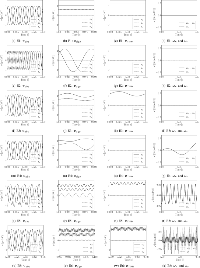
Figure 1: Examples E1-E6.

VI-A Balanced Three-Phase AC Voltages

The examples presented in this section utilize a balanced three-phase AC voltages in the form:

$$v_{a} =V\sin(\omega_{a}\,t+\theta_{a,0})\,,$$ (64)

$$v_{b} =V\sin(\omega_{a}\,t+\theta_{a,0}+\alpha)\,,$$

$$v_{c} =V\sin(\omega_{a}\,t+\theta_{a,0}-\alpha)\,,$$

where $\theta_{a,0}=\pi/6$ rad. The following four cases are considered:

• E1: $\omega_{\scriptscriptstyle\rm P}=\omega_{a}=\omega_{o}$, $V=15$ kV.

• E2: $\omega_{\scriptscriptstyle\rm P}=\omega_{o}$, $\omega_{a}=1.2\,\omega_{o}$ rad/s, $V=15$ kV.

• E3: $\omega_{\scriptscriptstyle\rm P}=\omega_{a}=\omega_{o}$, $V=15+3\sin(0.2\omega_{o}t)$ kV.

• E4: $\omega_{\scriptscriptstyle\rm P}=\omega_{o}$, $\omega_{a}=\omega_{o}+2\pi\sin(20\pi t)$ rad/s, $V=15$ kV.

The voltage $\boldsymbol{v}_{abc}$, $\boldsymbol{v}_{dqo}$, $\boldsymbol{v}_{\scriptscriptstyle\rm TNB}$ as well as the angular frequencies $\omega_{\kappa}$ and $\omega_{\tau}$ for the examples E1-E4 are shown in Figs. 1.(a)-(p).

Example E1 is the standard balanced, stationary case, for which the Park transform and the Frenet frame substantially coincide, except for the fact that the Frenet frame is independent from the angular position $\theta_{a,0}$. This is a consequence of the fact that the Frenet frame follows the voltage locally, whereas the Park transform follows an independent reference.

Example E2 shows one of the critical issues (especially, in the context of state estimation) of the Park transform: the fact that if $\omega_{\scriptscriptstyle\rm P}\neq\omega_{a}$ then, the Park $dq$-axis components oscillates at frequency $\omega_{a}-\omega_{\scriptscriptstyle\rm P}$, even if the amplitude of the measured signal is perfectly stationary [31]. As expected, on the other hand, the Frenet frame returns a steady-state voltage magnitude $v$ and azimuthal frequency $\omega_{\kappa}$.

Examples E3 and E4 represent dual scenarios. In E3, the voltage magnitude is time varying and the frequency is constant whereas, in E4, the voltage magnitude is constant and the angular frequency $\omega_{a}$ is time varying. The Park transform is unable to distinguish between these two situations, once again because of the constant external reference angular speed. On the other hand, the Frenet frame separates the effects of the variations of the voltage magnitude and of the angular frequency. It is relevant to observe that this property holds also for signals with time-varying voltage magnitude and angular frequency, which is the typical scenario in the first seconds of power system transients following a large disturbance (see the case study in Section VI-D).

VI-B Unbalanced Three-Phase AC Voltages

This section discusses the effect of unbalanced conditions. Let us define the following unbalanced three-phase AC voltages (example E5):

$$v_{a} =V\sin(\omega_{o}\,t+\theta_{a,0})\,,$$ (65)

$$v_{b} =1.2V\sin(\omega_{o}\,t+\theta_{a,0}+\alpha)\,,$$

$$v_{c} =0.8V\sin(\omega_{o}\,t+\theta_{a,0}-\alpha)\,,$$

where $\theta_{a,0}=\pi/6$ rad. The voltage $\boldsymbol{v}_{abc}$, $\boldsymbol{v}_{dqo}$, $\boldsymbol{v}_{\scriptscriptstyle\rm TNB}$ as well as the angular frequencies $\omega_{\kappa}$ and $\omega_{\tau}$ for the voltage vector (65) are shown in Figs. 1.(q)-(t).

The unbalanced conditions give birth to a non-null zero-sequence component in the vector $\boldsymbol{v}_{dqo}$. However, the curve associated with these conditions is still a plane curve, as confirmed by the fact that $\omega_{\tau}=0$. In turn, the trajectory described by the voltage is an ellipse rather than a circle. Then, to describe the curve it suffices to know only two quantities, not three as suggested by the Park transforms. This situation is properly captured by the Frenet frame: both the magnitude of the voltage and the azimuthal frequency are periodic, which reflects the fact that in ellipse, both the radius and the curvature are not constant and repeat periodically at every full turn.

VI-C Three-Phase AC Voltages with Harmonics

This example (E6) describes the effect of unbalanced harmonics on voltages transformed with the Park transform and the Frenet frame. We consider the following voltage vector:

$$v_{a} =V\,\{\sin(\omega_{o}\,t+\theta_{a,0})+0.1\,\sin[5(\omega_{o}\,t+\theta_{a,0})]\}\,,$$ (66)

$$v_{b} =V\,\{\sin(\omega_{o}\,t+\theta_{b,0})+0.2\,\sin[5(\omega_{o}\,t+\theta_{b,0})]\}\,,$$

$$v_{c} =V\,\{\sin(\omega_{o}\,t+\theta_{c,0})+0.1\,\sin[5(\omega_{o}\,t+\theta_{c,0})]\}\,,$$

where $V=15$ kV, $\theta_{a,0}=\pi/6$ rad, $\theta_{b,0}=\pi/6-\alpha$ rad, and $\theta_{c,0}=\pi/6+\alpha$ rad. The voltage $\boldsymbol{v}_{abc}$, $\boldsymbol{v}_{dqo}$, $\boldsymbol{v}_{\scriptscriptstyle\rm TNB}$ as well as the angular frequencies $\omega_{\kappa}$ and $\omega_{\tau}$ for the voltage vector (66) are shown in Figs. 1.(u)-(x).

Unbalanced harmonics leads to a time-varying torsional frequency $\omega_{\tau}$ (see also the examples included in [18]). It is relevant to note that, from the Park transform point of view, both E5 and E6 lead to a periodic $v_{o}$. Of course, the frequency of the oscillations allows distinguishing between E5 (unbalance voltages at the fundamental frequency) and E6 (harmonic content). However, only the Frenet frame allows interpreting correctly the “non-planar” nature of E6.

VI-D Power System Transient

This last example considers the IEEE 39-bus system. The model utilized in the simulation below is provided as an application example with DIgSILENT PowerFactory. This consists of a detailed EMT three-phase model. Beside machine and control dynamics of the original IEEE 39-bus benchmark system, the model includes the electromagnetic dynamics of transmission lines, transformers and synchronous machines. The contingency is a three-phase fault at bus 4. The fault occurs at $t=0.2$ s and is cleared at $t=0.3$ s. The time step of the numerical integration is $0.01$ ms. Figure 2 shows the trajectories of $\boldsymbol{v}_{abc}$, $\boldsymbol{v}_{dqo}$ and $\boldsymbol{v}_{\scriptscriptstyle\rm TNB}$ at bus 24 in pu with respect to a base of $220$ kV and of the azimuthal and torsional frequencies in pu with respect to $\omega_{o}=2\pi\,60$ rad/s.

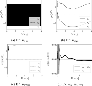
Figure 2: Example E7: Transient behavior of the voltage and frequency at bus 26 of the IEEE 39-bus system following a fault at bus 4.

The untransformed voltage vector $\boldsymbol{v}_{abc}$ carries “too much” information for the time scale of the simulation (several seconds), which is the typical one utilized to study electromechanical transients after a fault. This fully justifies the common practice to utilize a RMS model for the study of these transients. The Park-transformed voltage $\boldsymbol{v}_{dqo}$ suffers of the decoupling between the reference angular frequency utilized in $\boldsymbol{\rm P}(\omega_{o})$. The slip between the actual frequency at the bus and $\omega_{o}$ makes the interpretation of the behavior of the $dq$-axis components $v_{d}$ and $v_{q}$ not intuitive. The Frenet frame, on the other hand, provides straightforward information. The tangent component $v_{\scriptscriptstyle\rm T}$ is the time envelope of $\boldsymbol{v}_{abc}$. Then $\omega_{\kappa}$ shows the behavior of the local frequency at the bus. Finally, $\omega_{\tau}$, which is null except during the fault, indicates that the system does not include unbalanced harmonics.

On a practical note, the accuracy of the evaluation of the vectors of the Frenet frame as well as of the geometric invariants depends exclusively to the precision with which the time derivatives of the voltage can be evaluated. In fact, ${\scriptstyle\rm\boldsymbol{\rm T}}$ is the normalized three-phase ac voltage $\boldsymbol{v}_{abc}$, whereas ${\scriptstyle\rm\boldsymbol{\rm N}}$ and ${\scriptstyle\rm\boldsymbol{\rm B}}$ are obtained based on the first time derivative of $\boldsymbol{v}_{abc}$, see (50) and (51). Similarly $\omega_{\kappa}$ requires only the calculation of first time derivatives, whereas $\omega_{\tau}$ requires also second time derivatives, see (52) and (53). In this case study, the derivatives were obtained by numerically differentiating the sampled phase voltages at bus 26 and then removing noise with discrete butterworth and low-pass filters.

Finally, it is relevant to remark that, for a balanced case as the one discussed in this section, $v_{\scriptscriptstyle\rm N}=\sqrt{v_{d}^{2}+v_{q}^{2}}$ and $\omega_{\kappa}=\omega_{o}+\frac{d}{dt}\arctan(v_{q},v_{d})$. Moreover, the drift of the $dq$-axis components can be compensated by using the frequency of the center of inertia rather than $\omega_{o}$ in matrix $\boldsymbol{\rm P}$. However, the center of inertia is a quantity that can be calculated only in a computer simulation, not in practice. And, more importantly and as shown from examples E3 to E6, the Park transform does not always provide an easy way to interpret the results. The feature of decomposing the original voltage vector into meaningful quantities (invariants) is, by construction, specific only of the Frenet frame and constitutes thus its main advantage with respect to any other transforms.

VI-E Balanced Six-Phase Voltage

The Gram-Schmidt process described in Section IV-C is illustrated using a balanced six-phase system. Consider the following voltage vector:

$$\boldsymbol{v}=V\sum_{h=1}^{6}\sin\big{(}\omega_{o}t-(h-1)\beta\big{)}\boldsymbol{\rm e}_{\rm h}\,,$$ (67)

The first two orthonormal vectors of the Frenet frame are:

$$\tilde{\boldsymbol{\rm e}}_{1} =\frac{\boldsymbol{v}}{{|\boldsymbol{v}|}}\,\,\Rightarrow\,\,\boldsymbol{\rm f}_{1}=\frac{1}{\sqrt{3}}\sum_{h=1}^{6}\sin\big{(}\omega_{o}t-(h-1)\beta\big{)}\boldsymbol{\rm e}_{\rm h}\,,$$ (68)

$$\tilde{\boldsymbol{\rm e}}_{2} =\frac{\boldsymbol{v}^{\prime}}{{|\boldsymbol{v}|}^{2}}\,\,\Rightarrow\,\,\boldsymbol{\rm f}_{2}=\frac{1}{\sqrt{3}}\sum_{h=1}^{6}\cos\big{(}\omega_{o}t-(h-1)\beta\big{)}\boldsymbol{\rm e}_{\rm h}\,.$$

Then, note that $\boldsymbol{v}^{\prime\prime}=-\omega_{o}^{2}\boldsymbol{v}$ and $\boldsymbol{v}^{\prime\prime\prime}=-\omega_{o}^{2}\boldsymbol{v}^{\prime}$, etc. This indicates that the balanced six-phase voltage (67) is in effect a plane curve. The only nonnull remaining vector of the basis is thus the normalized vector perpendicular to both $\boldsymbol{\rm f}_{1}$ and $\boldsymbol{\rm f}_{2}$, namely:

$$\tilde{\boldsymbol{\rm e}}_{3}=\star(\boldsymbol{\rm f}_{1}\wedge\boldsymbol{\rm f}_{2})\,\,\Rightarrow\,\,\boldsymbol{\rm f}_{3}=\frac{1}{\sqrt{6}}\sum_{h=1}^{6}\boldsymbol{\rm e}_{i}\,.$$ (69)

The obtained Frenet frame $\boldsymbol{\rm F}=[\boldsymbol{\rm f}_{1},\boldsymbol{\rm f}_{2},\boldsymbol{\rm f}_{3}]$ is exactly the same 6-to-$dqo$ Park transform matrix proposed in [4]. The procedure utilized in [4], however, is more involved than the one proposed here as it utilizes the definition of groups. We have thus obtained that for a stationary balanced $n$-dimensional voltage vector the generalized Park transform is equivalent to the generalized Frenet frame. However, as expected, the Frenet frame is more general as it does not require the voltage to be balanced or stationary. Finally, we observe that $\omega_{\chi,1}=\omega_{o}$ and $\omega_{\chi,i}=0$ for $i=2,\dots,6$, which confirms that the curve lays on a plane.

VII Conclusions

The paper presents a geometrical interpretation of the Park transform, its time derivative and its generalization based on the Frenet frame and Cartan’s moving frames. The Frenet frame appears particularly relevant for the transient stability analysis of power systems for various reasons, as follows.

• The Frenet frame returns a set of geometric invariants which are as many as the phases of the circuit. These quantities represent fully and unequivocally the transient conditions of the voltage (or current) under consideration.

• The Frenet frame provides a natural phase angle reference as well as intrinsic angular frequency (namely the azimuthal frequency) for the voltage without the need for an external reference or a device that links to an external reference, such as the phase-locked loops.

• Cartan’s moving frame approach provides a systematic and general way to link the local Frenet frames to a common reference. The equations of such interfaces are duly provided in this work.

• The paper also shows how the Frenet frame can be extended to any number of phases and provides the steps required to calculate the generalized coordinates and curvatures for an arbitrary multi-phase circuit.

In the case study section, a variety of examples support the theory and show how the proposed approach solves the many idiosyncrasies of the Park transform.

The ability to identify the angular frequency of devices that do not have a rotor appears particularly promising for the study of converter-interfaced generation. Another relevant aspect is the practicality of the implementation of the proposed technique for on-line applications, such as control and dynamic state-estimation. These topics will be the focus of future work.

Federico Milano (F’16) received from the Univ. of Genoa, Italy, the ME and Ph.D. in Electrical Engineering in 1999 and 2003, respectively. From 2001 to 2002 he was with the University of Waterloo, Canada, as a Visiting Scholar. From 2003 to 2013, he was with the University of Castilla-La Mancha, Spain. In 2013, he joined the University College Dublin, Ireland, where he is currently a full professor. He is also Chair of the IEEE Power System Stability Controls Subcommittee, IET Fellow, IEEE PES Distinguished Lecturer, and Co-Editor in Chief of the IET Generation, Transmission & Distribution. His research interests include power system modeling, control and stability analysis.

References

- [1] R. H. Park, “Two-reaction theory of synchronous machines generalized method of analysis – Part I,” Transactions of the American Institute of Electrical Engineers, vol. 48, no. 3, pp. 716–727, 1929.
- [2] F. Milano and Á. Ortega, Frequency Variations in Power Systems: Modeling, State Estimation, and Control. Hoboken, NJ: Wiley, 2020.
- [3] A. Yazdani and R. Iravani, Voltage-Sourced Converters in Power Systems: Modeling, Control, and Applications. Hoboken, NJ: Wiley, 2010.
- [4] A. Z. Gaber and L. P. Singh, “Investigation of symmetries inherent in synchronous machines and development of a generalized Park’s transformation based solely upon symmetries,” Electric Power Systems Research, vol. 15, no. 3, pp. 203–213, 1988.
- [5] E. Levi, “Multiphase electric machines for variable-speed applications,” IEEE Transactions on Industrial Electronics, vol. 55, no. 5, pp. 1893–1909, 2008.
- [6] C. P. Steinmetz and E. J. Berg, Theory and Calculation of Alternating Current Phenomena. New York, US: W. J. Johnston Co., 1897.
- [7] J. C. Das, Power System Harmonics and Passive Filter Designs. Hoboken, NJ: IEEE Press – John Wiley & Sons, 2015.
- [8] C. L. Fortescue, “Method of symmetrical co-ordinates applied to the solution of polyphase networks,” Transactions of the American Institute of Electrical Engineers, vol. 37, no. 2, pp. 1027–1140, June 1918.
- [9] Y. H. Ku, “Transient analysis of A-C. machinery,” Transactions of the American Institute of Electrical Engineers, vol. 48, no. 3, pp. 707–714, July 1929.
- [10] E. Clarke, Circuit Analysis of AC Power Systems – Volume I: Symmetrical and Related Components, ser. General Electric Series. New York, US: J. Wiley & Sons, 1943.
- [11] A. M. Stanković and T. Aydin, “Analysis of asymmetrical faults in power systems using dynamic phasors,” IEEE Transactions on Power Systems, vol. 15, no. 3, pp. 1062–1068, Aug. 2000.
- [12] C. Liu, A. Bose, and P. Tian, “Modeling and analysis of HVDC converter by three-phase dynamic phasor,” IEEE Transactions on Power Delivery, vol. 29, no. 1, pp. 3–12, Feb. 2014.
- [13] N. N. Hancock, Matrix Analysis of Electrical Machinery, 2nd ed., ser. General Electric Series. New York, US: Pergamon Press, 1974.
- [14] J. J. Stoker, Differential Geometry. New York: Wiley-Interscience, 1969.
- [15] B. O’Neill, Elementary Differential Geometry. London: Academic Press, 1966.
- [16] L. Lapierre, D. Soetanto, and A. Pascoal, “Nonlinear path following with applications to the control of autonomous underwater vehicles,” in 42nd IEEE International Conference on Decision and Control, vol. 2, 2003, pp. 1256–1261.
- [17] M. Werling, J. Ziegler, S. Kammel, and S. Thrun, “Optimal trajectory generation for dynamic street scenarios in a Frenet frame,” in IEEE International Conference on Robotics and Automation, 2010, pp. 987–993.
- [18] F. Milano, G. Tzounas, I. Dassios, and T. Kërçi, “Applications of the Frenet frame to electric circuits,” IEEE Transactions on Circuits and Systems I: Regular Papers, vol. 69, no. 4, pp. 1668–1680, 2022.
- [19] F. Milano, “A geometrical interpretation of frequency,” IEEE Transactions on Power Systems, vol. 37, no. 1, pp. 816–819, 2022.
- [20] J. L. Willems, “Mathematical foundations of the instantaneous power concepts: A geometrical approach,” European Transactions on Electrical Power, vol. 6, no. 5, pp. 299–304, 1996.
- [21] X. Dai, G. Liu, and R. Gretsch, “Generalized theory of instantaneous reactive quantity for multiphase power system,” IEEE Transactions on Power Delivery, vol. 19, no. 3, pp. 965–972, 2004.
- [22] H. Lev-Ari and A. M. Stanković, “Instantaneous power quantities in polyphase systems – A geometric algebra approach,” in IEEE Energy Conversion Congress and Exposition, 2009, pp. 592–596.
- [23] H. Akagi, E. H. Watanabe, and M. Aredes, Instantaneous Power Theory and Applications to Power Conditioning, 2nd ed. New York: Wiley IEEE Press, 2017.
- [24] F. G. Montoya, R. Baños, A. Alcayde, F. M. Arrabal-Campos, and J. Roldán-Pérez, “Vector geometric algebra in power systems: An updated formulation of apparent power under non-sinusoidal conditions,” Mathematics, vol. 9, no. 11, 2021.
- [25] N. Barry, “The application of quaternions in electrical circuits,” in 2016 27th Irish Signals and Systems Conference (ISSC), 2016, pp. 1–9.
- [26] V. d. P. Brasil, A. de Leles Ferreira Filho, and J. Y. Ishihara, “Electrical three phase circuit analysis using quaternions,” in 18th International Conference on Harmonics and Quality of Power (ICHQP), 2018, pp. 1–6.
- [27] S. P. Talebi and D. P. Mandic, “A quaternion frequency estimator for three-phase power systems,” in IEEE International Conference on Acoustics, Speech and Signal Processing (ICASSP), 2015, pp. 3956–3960.
- [28] D. Fabozzi and T. Van Cutsem, “On angle references in long-term time-domain simulations,” IEEE Transactions on Power Systems, vol. 26, no. 1, pp. 483–484, Feb. 2011.
- [29] T. Needham, Visual Differential Geometry and Forms: A Mathematical Drama in Five Acts. Princeton, NJ: Princeton University Press, 2021.
- [30] F. Milano and Á. Ortega, “Frequency divider,” IEEE Transactions on Power Systems, vol. 32, no. 2, pp. 1493–1501, 2017.
- [31] M. Paolone et al., “Fundamentals of power systems modelling in the presence of converter-interfaced generation,” Electric Power Systems Research, vol. 189, p. 106811, 2020.