Camera Adaptation for Fundus-Image-Based CVD Risk Estimation

Abstract

Recent studies have validated the association between cardiovascular disease (CVD) risk and retinal fundus images. Combining deep learning (DL) and portable fundus cameras will enable CVD risk estimation in various scenarios and improve healthcare democratization. However, there are still significant issues to be solved. One of the top priority issues is the different camera differences between the databases for research material and the samples in the production environment. Most high-quality retinography databases ready for research are collected from high-end fundus cameras, and there is a significant domain discrepancy between different cameras. To fully explore the domain discrepancy issue, we first collect a Fundus Camera Paired (FCP) dataset containing pair-wise fundus images captured by the high-end Topcon retinal camera and the low-end Mediwork portable fundus camera of the same patients. Then, we propose a cross-laterality feature alignment pre-training scheme and a self-attention camera adaptor module to improve the model robustness. The cross-laterality feature alignment training encourages the model to learn common knowledge from the same patient’s left and right fundus images and improve model generalization. Meanwhile, the device adaptation module learns feature transformation from the target domain to the source domain. We conduct comprehensive experiments on both the UK Biobank database and our FCP data. The experimental results show that the CVD risk regression accuracy and the result consistency over two cameras are improved with our proposed method. The code is available here: https://github.com/linzhlalala/CVD-risk-based-on-retinal-fundus-images

1 Introduction

Cardiovascular diseases (CVD) are the leading causes of mortality around the world [17]. Early screening and identification of the at-risk populations are necessary for CVD prevention and control. The existing CVD risk estimation guidelines (for example, the WHO-CVD score [12]) are based on the patient physical measures and laboratory testing, such as body massive index (BMI) and high-density lipoprotein (HDL). However, some inputs are difficult to acquire in scenarios where medical professionals and laboratory testing are not accessible. A prospective solution is to predict fundus-image-based CVD risk with an automated CAD algorithm using a portable fundus camera. Recent studies [4, 16] have revealed the associations between the retinal fundus and its CVD risk factors. The fundus-image-based CVD risk estimation on a portable camera can significantly reduce the examination cost and the requirement of medical professionals. It will also improve medical democratization and let more people benefit from medical AI. Despite this prospective application, there still exist issues to be solved to achieve successful implementation. One of the most challenging problems is the domain discrepancy between fundus cameras. The ideal high-quality retinal samples for CVD risk inference are mainly captured by expensive clinical devices. For example, the retinal images from the UK Biobank [19] (UKB) are collected using the Topcon 3D OCT-1000 MKII. Meanwhile, the retinal samples in the practical scenario are sometimes captured by low-cost portable fundus cameras. The key components of the fundus camera, such as light source, lens, and camera sensor, are all different. The impacts on images quality and style can lead to the problem of domain discrepancy.

To tackle the problem of fundus camera adaptation, the existing efforts have mainly focused on feature and image alignment. The CFEA [14] exploited collaborative adversarial learning and self-ensembling for feature adaptation on the optic disc (OD) and optic cup (OC) segmentation task. The CSFA [13] concentrated on the content and style feature consistency among source domain images, target-like query images and target domain images also for the disc and cup segmentation task. Yang et al. [21] proposed a camera-oriented residual-CycleGAN to pre-process the images and improve the diabetic retinopathy prediction performance on multiple cameras data. Ju et al. [11] proposed a modified CycleGAN to bridge the domain gap between regular and ultra-widefield fundus images for several tasks. However, these solutions only consider the target domain performance with abundant training images from the target domain required, which is impossible to collect in our task. Furthermore, these methods also ignore the cross-domain consistency, which may lead to disastrous outcomes for CVD risk evaluation.

In this work, we collect a Fundus Camera Paired (FCP) dataset containing the pair-wise fundus images of the same patients using two cameras (Topcon upright camera and Mediwork portable camera). Our strategy on the task is two-fold: domain generalization [20] and domain adaptation [9]. The domain generalization is to improve the adaptability with the unseen target domain. Inspired by the contrastive learning [2, 3, 8], we propose a cross-laterality feature alignment (CLFA) pre-training scheme to utilize the images of both lateralities, which are believed to share the invariant representation for the CVD risk. Besides the supervised CVD risk regression, we introduce an asymmetric feature alignment task for domain generalization by comparing the pair-wise image features and letting the superior one teach the other one to enhance the learning on domain-invariant representation. Domain adaptation is to adapt the model to the target domain given. To maintain the model knowledge on the CVD task, we adopt a plug-in camera adaptor module based on multi-head self-attention. The camera adaptor can transform the target domain image feature to match its source domain edition. The experiment shows that our two-step strategy improves the CVD risk regression performance on the UKB dataset and the prediction consistency between the two cameras on our FCP dataset. Moreover, we conduct ablation studies on our pre-training method and camera adaptor. We find that our CLFA pre-training reduces the feature-space discrepancy between the UKB dataset and the other cameras. Meanwhile, our camera adaptor can significantly improve the CVD result coefficient on different pre-trained models.

2 Method

2.1 Cross-Laterality Feature Alignment Pre-training

Our cross-laterality feature alignment (CLFA) pre-training is inspired by the domain generalization research [20] and contrastive learning [8, 2, 3]. The UKB provides both left and right fundus photos for each patient, which can be utilized as natural positive sample pairs. We hypothesize that the visual clues of CVD risk have invariant representation over the two eyes. A deep learning model would have better generalization when identifying the invariant representation. As shown in Fig.1, our pre-training adopts the siamese network [5] and lets both lateralities share the backbone model (a vision transformer model in this paper). The model is simultaneously trained with two branches.

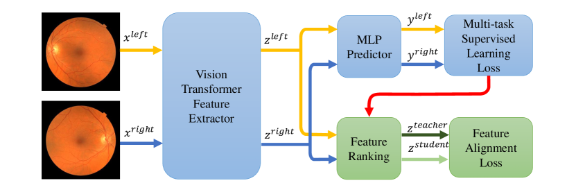
Figure 1: The cross-laterality feature alignment pre-training has two branches: a multi-task supervised learning branch and an asymmetric feature alignment branch.

In the supervised learning branch, we jointly train the model on the WHO-CVD score as well as seven clinical variables explicitly related to the WHO-CVD, including age, systolic blood pressure (SBP), total cholesterol (TC), body massive index (BMI), gender, smoking status, and diabetes status. The aim is to improve the model generalization by sharing representations between the tasks [22]. Let $S=\left\{x_{i}^{left},x_{i}^{right},y_{i}^{rgs},y_{i}^{cls}\right\}_{i=1}^{n}(rgs=1,2,3,4,5;cls=1,2,3)$ denote the training set, where the $x_{i}^{left}$ denotes the left fundus photo, $x_{i}^{right}$ denotes the right fundus photo, $y_{i}^{rgs}$ denotes the regression labels, and $y_{i}^{cls}$ denotes the binary classification labels. The backbone model is defined as the function of $f_{\theta}:\mathcal{X}\rightarrow(\mathcal{Y}^{rgs},\mathcal{Y}^{cls})$. The mean squared error (MSE) and binary cross-entropy (BCE) are used as the loss functions for the regression and binary classification. The weighting of tasks are denoted as $W=\left\{w^{rgs},w^{cls}\right\}(r=1,2,...,5;c=1,2,...,3)$. The $\sigma(\cdot)$ denotes the $sigmoid$ function. The loss function of branch is defined as follows:

$$\begin{split}\ell_{sup.}(\theta)=\sum_{rgs=1}^{5}w^{rgs}\cdot MSE\Big{(}y_{i}^{rgs},f_{\theta}^{rgs}(x_{i})\Big{)}+\sum_{cls=1}^{3}w^{cls}\cdot BCE\Big{(}y_{i}^{cls},\sigma(f_{\theta}^{cls}(x_{i}))\Big{)}\end{split}$$ (1)

Note that both eyes are used as laterality-agnostic inputs. Hence, for every patient we have two supervised loss $\{\ell_{sup.}^{left},\ell_{sup.}^{right}\}$.

The feature alignment learning branch is designed to enable the interaction between two fundus image features from the same patient. With the input pair $\{x_{i}^{left},x_{i}^{right}\}$, the two supervised learning loss $\{\ell_{sup.}^{left},\ell_{sup.}^{right}\}$ will have a larger one and a smaller one. The feature with the smaller loss is selected as the teacher while the other is selected as the student. This operation can be regarded as a feature-level knowledge distillation. The backbone model function can be split into two steps: the feature extractor function $g_{\theta}:\mathcal{X}\rightarrow\mathcal{Z}$ and the predict function $p_{\theta}:\mathcal{Z}\rightarrow(\mathcal{Y}^{rgs},\mathcal{Y}^{cls})$. The $SD(\cdot)$ means the stop-gradient operation. The loss function is defined as follows:

$$\ell_{ali.}(\theta)=\begin{cases}MSE\big{(}g_{\theta}(x_{i}^{l}eft),SD(g_{\theta}(x_{i}^{r}iht))\big{)}&\ell_{sup.}^{left}\geq\ell_{sup.}^{right},\\ MSE\big{(}g_{\theta}(x_{i}^{r}ight),SD(g_{\theta}(x_{i}^{l}eft))\big{)}&\ell_{sup.}^{left}<\ell_{sup.}^{right}\end{cases}$$ (2)

Hence the overall loss function of the CLFA pre-training is as follows, where the $\lambda$ denotes the weighting for the feature alignment branch:

$$L_{S}(\theta)=L_{S}^{sup.}(\theta)+\lambda\cdot L_{S}^{ali.}(\theta)$$ (3)

2.2 Self-Attention Camera Adaptor Module

Our self-attention camera adaptor (SACA) module is inspired by the feature learning approaches [9] in domain adaptation research. We freeze the pre-trained model to anchor the outcome of the source domain. Meanwhile, we add an adaptor module for the target domain. This strategy allows us to utilize the pairing information in our FCP dataset and establish the benchmark based on cross-domain consistency.

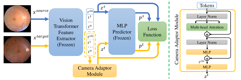
Figure 2: The left part of the figure illustrates the workflow of prediction. The blue arrows represent the prediction procedure of the source domain, while the yellow arrows represent the prediction procedure of the target domain. The right part of the figure shows the structure of the camera adaptor module.

The module network is shown in Fig.2. Based on our early performance comparison, we choose the vision transformer [6] (ViT) as our backbone model. The ViT feature extractor outputs the classification token and image patch tokens as $T^{out}=\left\{t^{cls},t^{1},t^{2},...,t^{N}\right\}$. Generally, the classification token ($t^{cls}$) is used as the image feature (denoted as $\mathcal{Z}$ in the Sec. 2.1). However, the image patch embeddings are also informative and can be utilized in our task. We adopt the block design of ViT, including the multiheaded self-attention (MSA), multilayer perceptron (MLP), Layernorm (LN), and residual connections. Besides the block, we apply an extra MLP projector. The camera adaptor module ($k_{\beta}:T\rightarrow\mathcal{Z}_{a}$) can be described as follow:

$$\begin{split}&{T}^{\prime}=MSA(LN(T_{out}))+T_{out}\\ &T_{a}=MLP(LN({T}^{\prime}))+{T}^{\prime}=\left\{t_{a}^{cls},t_{a}^{1},t_{a}^{2},...,t_{a}^{N}\right\}\\ &\mathcal{Z}_{a}=MLP(t_{a}^{cls})\end{split}$$ (4)

To train the camera adaptor module, we use pair-wise data which is denoted as $P=\left\{x_{i}^{s},x_{i}^{t}\right\}_{i=1}^{n}$. For each image pair $\left\{x^{s},x^{t}\right\}$ fed in the source model and the adapted model, we have the WHO-CVD prediction $\left\{p^{s},p^{t}\right\}$. We define the training loss function as:

$$\begin{split}L_{P}(\beta)=\frac{1}{n}\sum_{i=1}^{N}MSE\Big{(}p_{i}^{s},p_{i}^{t}\Big{)}\end{split}$$ (5)

3 Experiment

3.1 Dataset

In this work, we use the UK Biobank retinal photography dataset (UKB) [19] for backbone model pre-training and our Fundus Camera Paired (FCP) dataset for camera adaptor training and evaluation. The UKB originally had 58,700 patients, and the images were captured by a Topcon 3D OCT-1000 MKII camera. We conduct an image quality assessment and a clinical information assessment. The selected 41,530 patients are split into 33,224 for training and 8,306 for validation balanced by the WHO-CVD score. From the validate split, we slice a balanced subset (UKB*) of 416 patients (741 images) for the feature distribution study. The FCP dataset has 227 patients and 415 pairs of pair-wise photos captured by Topcon TRC-NW8 camera and the Mediwork FC-162 portable camera. The patients are split into 182 for training and 45 for validation randomly. There is no patient information collected in the FCP dataset.

3.2 Implementation Details and Metrics

For the UKB dataset, we calculate the WHO-CVD score according to the WHO guideline [12] and transform it into the logarithmic scale to normalize the distribution. Our backbone vision transformer (ViT) model structure is as the “R26+S/32” in the AugReg [18]. The model loads the ImageNet pre-trained [18] as the initial state. The default task weighting $w^{c},w^{r},\lambda$ mentioned in Sec.2.1 are all set to 1.0 for default. For backbone model pre-training, the batch size is 16, and the start learning rate is 1e-4. The augmentation includes resize, crop, color jitter, and grayscale. For the camera adaptor module, the batch size is 32, and the start learning rate is 1e-2. All experiments in this study use the Adam optimizer with momentum 0.9 and weight decay 1e-4.

coefficient of determination ($R^{2}$) is used to evaluate the WHO-CVD regression performance and the WHO-CVD result consistency between cameras with the Topcon result as pseudo target and the Mediwork result as the prediction. We also experimentally introduce the Multi-Kernel Maximum Mean Discrepancy (MK-MMD) [7] to measure the feature-distribution discrepancy between domains.

3.3 Ablation Study

We perform an ablation study to show the effectiveness of each design in our backbone model pre-training and camera adaptation.

3.3.1 Backbone Model Pre-training

In this experiment, we pre-train several backbone models on the UKB dataset and then train the camera adaptor  for each backbone model. Tab. 1 shows our experiment result of the backbone model pre-training. The baseline model is the ViT model with only the supervised learning branch and the WHO-CVD regression task. In “Weight1” the eight tasks describe in Sec. 2.1 are equally weighted. With “Weight1”, we observe the $R^{2}_{CVD}$ degrades and the $R^{2}$ scores of systolic blood pressure (SBP), total cholesterol (TC), and body massive index (BMI) regression are very low. Therefore, in “Weight2,” we remove the SBP, TC, BMI and increase the weight of WHO-CVD and achieve an increased $R^{2}_{CVD}$. Based on the “Weight2” supervised learning branch, we add the second branch of contrastive learning [2] or our Cross-Laterality Feature Alignment (CLFA). Surprisingly, the “Weight2+SimSiam” has obtained a collapsing performance while the “Weight2+CLFA” achieves the highest $R^{2}_{CVD}$ and post-adaptation $R^{2}_{(T,M)}$. It indicates that our “Weight2+CLFA” provides the best potential and adaptability. The MK-MMD comparison shows the “Weight2+CLFA” has the lowest feature-distribution discrepancy between UKB and Mediwork as well as between UKB and Topcon. These two variables show a negative correlation to the $R^{2}_{(T,M)}$. However, the pre-adaptation $R^{2}_{(T,M)}$ and feature-distribution discrepancy between Topcon and Mediwork shows no strong relation to post-adaptation $R^{2}_{(T,M)}$. The relation between MK-MMD and post-adaptation $R^{2}_{(T,M)}$ indicates the MK-MMD can be a metric to evaluate model adaptability in future research.

Table 1: Ablation study on the pre-training (CVD=WHO-CVD Regression on the UKB; T=Topcon data in FCP; M = Mediwork data in FCP; U* = A balanced subset of the UKB validate set.)

Method	$R^{2}_{CVD}$	$R^{2}_{(T,M)}$		MK-MMD (Pre-Ada.)
		Pre-ada.	Post-ada.	T$\leftrightarrow$M	U*$\leftrightarrow$M	U*$\leftrightarrow$T
Baseline	0.5586	0.3610	0.4071	0.3028	0.4898	0.1836
Weight1	0.5319	0.3263	0.4373	0.3996	0.3789	0.3372
Weight2	0.5643	0.1572	0.4176	0.3456	0.3972	0.2333
Weight2+SimSiam	0.0267	-0.0128	0	0.0002	4.2678	0.0003
Weight2+CLFA	0.5703	0.2144	0.4937	0.3741	0.3557	0.1597

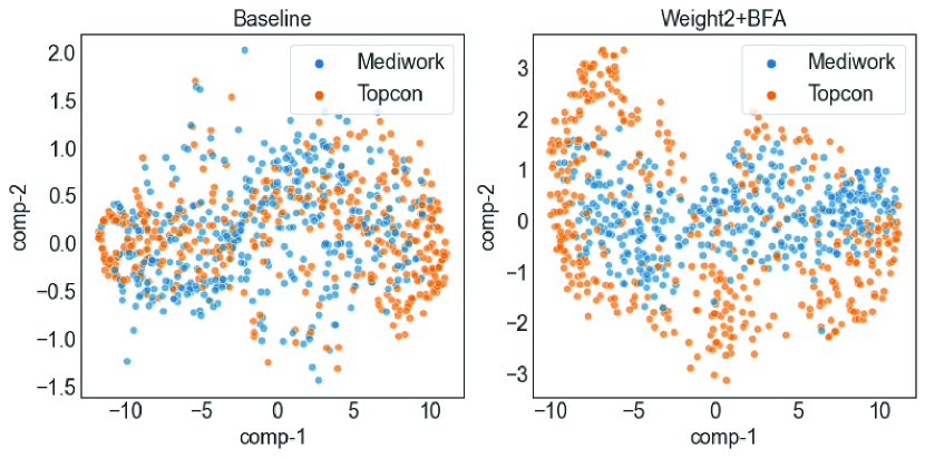
(a) The t-SNE features visualization on the FCP dataset

Model	$AUC_{lat.}$	$AUC_{camera}$
Baseline	0.5270	0.6414
Weight2+CLFA	0.7322	0.9722

(b) Laterality and camera prediction performance on the FCP dataset

Figure 3: Study of features extracted from the pre-training models

To further investigate the factors for model adaptability, we visualize the image feature of the FCP dataset extracted by “Baseline” and “Weight2+CLFA” through t-SNE as shown in Fig. 3(a). We figure out “Weight2+CLFA” has better feature clustering over different cameras. To quantify this observation, we train a single layer fully connected neural network on the image feature to predict the eye laterality and camera. The result is as Tab. 3(b), and it proves the “Weight2+CLFA” feature can support better discrimination of laterality and camera. Furthermore, it indicates that discrimination on camera may positively affect post-adaptation result consistency.

Table 2: Ablation study on the camera adaptor (SA=Self-attention.)

Module	$R^{2}(T,{M})$
	$\ell_{CVD}$	$\ell_{feature}$	$\ell_{MK-MMD}$	$\ell_{CVD}+\ell_{feature}$
MLP	0.3831	0.3479	0.1349	0.3602
SA Block	0.3229	0.3097	0.3052	0
SA Block+MLP	0.4937	0.4885	0.2113	0.3458

3.3.2 Camera Adaptor Module

To verify the design of our camera adaptor module, we test it under several different settings with a range of loss functions. The results in Tab. 2 demonstrate that both the self-attention block and the MLP projector are essential for our camera adaptor module. The comparison of the loss function shows that the WHO-CVD score-focused loss function has the best results. We also observe that optimizing the feature distribution discrepancy (MK-MMD) between features does not improve the prediction result consistency.

3.4 Quantitative Analysis

Table 3: The overall performance comparison (CVD = WHO-CVD regression on UKB; T=Topcon data in FCP; M = Mediwork data in FCP.)

Method	$R^{2}$(CVD)	$R^{2}(T,{M})$
Baseline	0.5586	0.3610
Baseline+DAN [15]	0.5586	0.3243
Baseline+DANN [1]	-0.0253	0.0254
Baseline+MDD [23]	-0.0104	1.000
Baseline+Pix2Pix GAN [10]	0.5586	0.3183
Baseline+Cycle GAN [24]	0.5586	0.3594
Ours (CLFA Pre-training + Adaptation Module)	0.5703	0.4732

To compare our proposed method and other approaches, we select several typical approaches of feature-alignment and image-alignment. The baseline model in this experiment is as Sec. 3.3.1 and is without the adaptor. For feature-alignment, we test the DAN [15] which optimize the MK-MMD between transformed features, the DANN [1] which apply the adversairal training, and the MDD [23] which using an auxiliary classifier to optimize the discrepancy between the two domains. For image alignment, we select the Pix2Pix GAN [10] and Cycle GAN [24] as the generators. The comparison shows that our method improves the result consistency over the two cameras. However, DAN, DANN, Cycle GAN, and Pix2Pix GAN lead to a lower consistency than baseline. The MDD reach $R^{2}=1.0$ as the model output a collapsed result. For the DAN, the reason for degrading may be DAN is designed for unpaired data and its MK-MMD-based loss function have no advantage when pair-wise data is available, which has also been proved in our ablation study (Sec. 2). The DANN and MDD require the parameter updating on the backbone model and lead to the degrading of backbone model. For the Pix2Pix GAN, we check its generated images and find the generator focusing on color toning or image style adjustment with a loss of the microvascular vessels’ detail, which is supposed to be an essential visual representation of CVD. The Cycle GAN learns some image style transformation but fails to improve the predcition outcome. The advantage of our CLFA pre-training plus camera adaptor method is that both generalization and adaptation are considered to improve the model’s adaptability.

4 Conclusion

This paper researches the domain discrepancy problem in developing a fundus-image-based CVD risk predicting algorithm. We observe that the deep learning model trained conventionally will have a variant representation on photos from different fundus cameras. Therefore, we propose a cross-laterality feature learning training method and a camera adaptor module. The experiments show that our design has improved on the prediction result consistency. Also, we find that the feature-space distribution discrepancy between pre-training and target domain data may be the key factor of model transportability. Future research will explore the data augmentation in adaption to overcome the data lacking and utilize the FCP data in the backbone model pre-training.

References

- [1] Ajakan, H., Germain, P., Larochelle, H., Laviolette, F., Marchand, M.: Domain-adversarial neural networks. arXiv preprint arXiv:1412.4446 (2014)
- [2] Chen, X., He, K.: Exploring simple siamese representation learning. In: IEEE Conference on Computer Vision and Pattern Recognition, CVPR 2021, virtual, June 19-25, 2021. pp. 15750–15758. Computer Vision Foundation / IEEE (2021)
- [3] Chen*, X., Xie*, S., He, K.: An empirical study of training self-supervised vision transformers. arXiv preprint arXiv:2104.02057 (2021)
- [4] Cheung, C.Y., Thomas, G.N., Tay, W., Ikram, M.K., Hsu, W., Lee, M.L., Lau, Q.P., Wong, T.Y.: Retinal vascular fractal dimension and its relationship with cardiovascular and ocular risk factors. American journal of ophthalmology 154(4), 663–674 (2012)
- [5] Chicco, D.: Siamese neural networks: An overview. Artificial Neural Networks pp. 73–94 (2021)
- [6] Dosovitskiy, A., Beyer, L., Kolesnikov, A., Weissenborn, D., Zhai, X., Unterthiner, T., Dehghani, M., Minderer, M., Heigold, G., Gelly, S., Uszkoreit, J., Houlsby, N.: An image is worth 16x16 words: Transformers for image recognition at scale. In: 9th International Conference on Learning Representations, ICLR 2021, Virtual Event, Austria, May 3-7, 2021. OpenReview.net (2021)
- [7] Gretton, A., Sejdinovic, D., Strathmann, H., Balakrishnan, S., Pontil, M., Fukumizu, K., Sriperumbudur, B.K.: Optimal kernel choice for large-scale two-sample tests. Advances in neural information processing systems 25 (2012)
- [8] Grill, J., Strub, F., Altché, F., Tallec, C., Richemond, P.H., Buchatskaya, E., Doersch, C., Pires, B.Á., Guo, Z., Azar, M.G., Piot, B., Kavukcuoglu, K., Munos, R., Valko, M.: Bootstrap your own latent - A new approach to self-supervised learning. In: Larochelle, H., Ranzato, M., Hadsell, R., Balcan, M., Lin, H. (eds.) Advances in Neural Information Processing Systems 33: Annual Conference on Neural Information Processing Systems 2020, NeurIPS 2020, December 6-12, 2020, virtual (2020)
- [9] Guan, H., Liu, M.: Domain adaptation for medical image analysis: a survey. IEEE Transactions on Biomedical Engineering (2021)
- [10] Isola, P., Zhu, J.Y., Zhou, T., Efros, A.A.: Image-to-image translation with conditional adversarial networks. In: Proceedings of the IEEE conference on computer vision and pattern recognition. pp. 1125–1134 (2017)
- [11] Ju, L., Wang, X., Zhao, X., Bonnington, P., Drummond, T., Ge, Z.: Leveraging regular fundus images for training uwf fundus diagnosis models via adversarial learning and pseudo-labeling. IEEE Transactions on Medical Imaging 40(10), 2911–2925 (2021). https://doi.org/10.1109/TMI.2021.3056395
- [12] Kaptoge, S., Pennells, L., De Bacquer, D., Cooney, M.T., Kavousi, M., Stevens, G., Riley, L.M., Savin, S., Khan, T., Altay, S., et al.: World health organization cardiovascular disease risk charts: revised models to estimate risk in 21 global regions. The Lancet Global Health 7(10), e1332–e1345 (2019)
- [13] Lei, H., Liu, W., Xie, H., Zhao, B., Yue, G., Lei, B.: Unsupervised domain adaptation based image synthesis and feature alignment for joint optic disc and cup segmentation. IEEE Journal of Biomedical and Health Informatics 26(1), 90–102 (2022). https://doi.org/10.1109/JBHI.2021.3085770
- [14] Liu, P., Kong, B., Li, Z., Zhang, S., Fang, R.: Cfea: collaborative feature ensembling adaptation for domain adaptation in unsupervised optic disc and cup segmentation. In: International Conference on Medical Image Computing and Computer-Assisted Intervention. pp. 521–529. Springer (2019)
- [15] Long, M., Cao, Y., Wang, J., Jordan, M.: Learning transferable features with deep adaptation networks. In: International conference on machine learning. pp. 97–105. PMLR (2015)
- [16] Poplin, R., Varadarajan, A.V., Blumer, K., Liu, Y., McConnell, M.V., Corrado, G.S., Peng, L., Webster, D.R.: Prediction of cardiovascular risk factors from retinal fundus photographs via deep learning. Nature Biomedical Engineering 2(3), 158–164 (2018)
- [17] Roth, G.A., Mensah, G.A., Johnson, C.O., Addolorato, G., Ammirati, E., Baddour, L.M., Barengo, N.C., Beaton, A.Z., Benjamin, E.J., Benziger, C.P., et al.: Global burden of cardiovascular diseases and risk factors, 1990–2019: update from the gbd 2019 study. Journal of the American College of Cardiology 76(25), 2982–3021 (2020)
- [18] Steiner, A., Kolesnikov, A., Zhai, X., Wightman, R., Uszkoreit, J., Beyer, L.: How to train your ViT? data, augmentation, and regularization in vision transformers. CoRR abs/2106.10270 (2021)
- [19] Sudlow, C., Gallacher, J., Allen, N., Beral, V., Burton, P., Danesh, J., Downey, P., Elliott, P., Green, J., Landray, M., et al.: Uk biobank: an open access resource for identifying the causes of a wide range of complex diseases of middle and old age. PLoS medicine 12(3), e1001779 (2015)
- [20] Wang, J., Lan, C., Liu, C., Ouyang, Y., Zeng, W., Qin, T.: Generalizing to unseen domains: A survey on domain generalization. arXiv preprint arXiv:2103.03097 (2021)
- [21] Yang, D., Yang, Y., Huang, T., Wu, B., Wang, L., Xu, Y.: Residual-cyclegan based camera adaptation for robust diabetic retinopathy screening. In: International Conference on Medical Image Computing and Computer-Assisted Intervention. pp. 464–474. Springer (2020)
- [22] Zhang, Y., Yang, Q.: A survey on multi-task learning. IEEE Transactions on Knowledge and Data Engineering (2021)
- [23] Zhang, Y., Liu, T., Long, M., Jordan, M.: Bridging theory and algorithm for domain adaptation. In: International Conference on Machine Learning. pp. 7404–7413. PMLR (2019)
- [24] Zhu, J.Y., Park, T., Isola, P., Efros, A.A.: Unpaired image-to-image translation using cycle-consistent adversarial networks. In: Proceedings of the IEEE international conference on computer vision. pp. 2223–2232 (2017)