Complex Generalized Integral Means Spectrum of Drifted Whole-Plane SLE & LLE

Abstract.

We present new exact results for the complex generalized integral means spectrum (in the sense of [DHLZ18]) for two kinds of whole-plane Loewner evolutions driven by a Lévy process:

• The case of a Lévy process with continuous trajectories, which corresponds to Schramm-Loewner evolution SLE_κ with a drift term in the Brownian driving function. There is no known result for its standard integral means spectrum, and we show that a natural path to access it goes through the introduction of the complex generalized integral means spectrum, which is obtained via the so-called Liouville quantum gravity.

• The case of symmetric Lévy processes for which we generalize results by Loutsenko and Yermolayeva ([Lou12, LY13, LY14, LY19]).

Dedicated to the Memory of Krzysztof Gawedzki

1. Introduction

“Il apparut que, entre deux vérités du domaine réel, le chemin le plus facile et le plus court passe bien souvent par le domaine complexe.”[It came to appear that, between two truths of the real domain, the easiest and shortest path quite often passes through the complex domain] (Paul Painlevé, 1900) [Pai00].

More than two decades ago, Oded Schramm [Sch00] introduced his celebrated theory of random growth processes SLE_κ. As an example, in the so-called chordal case in the half-plane $\mathbb{H}$, it consists of the one-parameter family of Loewner processes driven on the real line $\partial\mathbb{H}$ by $\sqrt{\kappa}B_{t}$, where $\kappa$ is a nonnegative number and $B_{t}$ is standard one-dimensional Brownian motion. This is the unique family of random processes satisfying a certain Markov property with continuous driving function, that is symmetric with respect to the imaginary axis. This theory may be generalized along two directions:

1. One can drop symmetry with respect to the imaginary axis: one then considers SLE_κ with a drift term, e.g., the chordal Loewner process driven by a random function of the form

   $$\lambda(t)=\sqrt{\kappa}B_{t}+at,$$

   where $B_{t}$ is as before standard one-dimensional Brownian motion and $a\in{\mathbb{R}}$.

2. One can drop the continuity assumption while keeping symmetry: the process so obtained is Loewner evolution driven by a Lévy process, called LLE (for Lévy-Loewner evolution).

Notice that the first class of continuous drifted processes coincides with the whole class of LLE processes with continuous trajectories. For $\kappa=0$, the Loewner process generated by $\lambda(t)=at$ becomes deterministic. Several deterministic chordal Loewner processes, driven by Lip-$1/2$ functions, were investigated in [KNK04, MR05, Lin05, LMR10].

In this paper, we shall consider both extended classes in the whole-plane case. In order to understand the multifractal spectra of these processes, such as their integral means spectra (ims), and in the spirit of references [DNNZ15, DHLZ18, Ho16, Lou12, LY13, LY14, LY19], we shall first investigate the cases for which the expected complex moments,

$$\mathbb{E}\left[|f^{\prime}(z)^{p}|\left|\left(\frac{z}{f(z)}\right)^{q}\right|\right],\,\,p,q\in\mathbb{C},$$

may be computed explicitly, to become part of integrable probability. Here $f$ stands for the time $0$ whole-plane map from $\mathbb{D}$ to the slit plane in the corresponding Loewner process. Note that complex values of $(p,q)$ are considered here in the case of whole-plane SLE with drift. In agreement with the citation by P. Painlevé above, the suggested passage by the complex plane will help us discover the precise form of the associated integral means spectrum in the case of SLE_κ with drift, via its complex and generalized versions [DHLZ18].

In Section 2, we shall make use of the so-called Liouville quantum gravity and Coulomb gas techniques, in the spirit of [Dup00, DB02, Dup04, DMS21], to (non-rigorously) derive the full complex generalized integral means spectrum $\beta_{1}(p,q;\kappa,a)$ of whole-plane SLE_κ with drift $a$ and for $(p,q)\in\mathbb{C}^{2}$. Section 3 covers SLE integrable cases, which are rigorously solved on a two-dimensional sub-manifold of $\mathbb{C}^{2}$ which generalizes the integrable parabolae of [DHLZ18] and [Ho16], and successfully compared with the previous claims. For the generalized spectrum of LLE processes studied in Section 4, we shall concentrate on $(p=2,q\in\mathbb{R})$ integrable cases, which can be solved analytically by closing some recursions between Fourier modes, in the spirit of [LY19].

The remainder of the present introductory Section 1 is devoted to providing precise definitions, and as a warm-up, to computing the complex generalized spectrum of the logarithmic spiral, in the first $(p,q)\in\mathbb{C}^{2}$, $\kappa=0,a\neq 0$ non-trivial case.

1.1. Interior whole-plane SLE

SLE is a particular case of a growth process called the Loewner process, of which several variants exist, known as chordal, radial, dipolar, or whole-plane [Law05, Bel19]. In this work we will consider the interior whole-plane case, which is determined by a driving function $\lambda:[0,+\infty)\to\partial\mathbb{D}:=\{z\in\mathbb{C}:|z|=1\}$ obtained as follows. Let us start by defining $\gamma:\,[0,+\infty)\to\mathbb{C}$ to be a continuous function such that $\lim_{t\to+\infty}|\gamma(t)|=+\infty$ and $\gamma(t)\neq 0,\forall t\geq 0$. Then, for each $t>0$, the slit domain $\Omega_{t}=\mathbb{C}\backslash\gamma([t,\infty))$ is a simply connected domain containing $0$. By the Riemann Mapping Theorem, there exists a unique conformal map $f_{t}:\mathbb{D}\to\Omega_{t}$ such that $f_{t}(0)=0$ and $f_{t}^{\prime}(0)>0$. By the Caratheodory convergence theorem, $f_{t}$ converges to $f_{0}$, the Riemann mapping of $\Omega_{0}$, as $t\to 0$. We may assume without loss of generality that $f_{0}^{\prime}(0)=1$ and, by re-parametrizing the curve if necessary, choose the normalization $f_{t}^{\prime}(0)=e^{t}$. Loewner’s theorem asserts that there exists a continuous function $\lambda$ taking values in the unit circle such that

$$\frac{\partial}{\partial t}f_{t}(z)=z\frac{\partial}{\partial z}f_{t}(z)\frac{\lambda(t)+z}{\lambda(t)-z},\,\,\,\,\lim\limits_{t\rightarrow+\infty}f_{t}(e^{-t}z)=z,\forall z\in\mathbb{D}.$$ (1.1)

The Loewner method can be reversed: given a continuous function $\lambda:[0,+\infty)\rightarrow\partial\mathbb{D}$, the partial differential equation (1.1) has a unique solution $f_{t}(z)$, which is a conformal map from $\mathbb{D}$ onto a domain $\Omega_{t}$, and the corresponding family $(\Omega_{t})_{t}$ is increasing in $t$. Nevertheless the domains $\Omega_{t}$ need not be slit domains as in the example above.

Whole-plane SLE_κ is the process driven by

$$\lambda(t)=e^{i\sqrt{\kappa}B_{t}},$$

where $\kappa\in[0,+\infty)$ and $B_{t}$ is standard one-dimensional Brownian motion. Note that when $\kappa=0$, $f_{t}(z)=\frac{e^{t}z}{(1-z)^{2}}$ is the solution to (1.1), so that $f_{0}$ is the Koebe function. Thus, as $\kappa\to 0^{+}$, whole-plane SLE_κ may be seen as a stochastic perturbation of the Koebe map.

In this work, we generalize SLE by adding a drift term to Brownian motion, with a driving function defined as

$$\lambda(t):=e^{i(\sqrt{\kappa}B_{t}+at)},a\in\mathbb{R}.$$ (1.2)

The process driven by $\lambda(t)$ then appears for small $\kappa$ as a stochastic perturbation of the $(\kappa=0,\,\,a\neq 0)$ case of the logarithmic spiral.

1.2. Complex generalized integral means spectrum

Let $f$ be a conformal map from $\mathbb{D}$ to $\mathbb{C}$ with $f(0)=0,f^{\prime}(0)=1$. The generalized integral means spectrum of $f$ was originally defined in [DHLZ18] as follows: for any pair of real numbers $(p,q)$, define the integral moments, for $r\in[0,1)$,

$$M_{f}(p,q):=\int_{0}^{2\pi}r^{q}\frac{|f^{\prime}(re^{i\theta})|^{p}}{|f(re^{i\theta})|^{q}}d\theta,\,\,r\in[0,1).$$ (1.3)

The generalized integral means spectrum is then defined as

$$\beta_{f}(p,q):=\limsup_{r\to 1^{-}}\left[\log M_{f}(p,q)/\log\left((1-r)^{-1}\right)\right].$$

If the limit exists, then

$$M_{f}(p,q)\stackrel{{\scriptstyle\cdot}}{{\sim}}\left(1-r\right)^{-\beta_{f}(p,q)},\,\,\,r\to 1^{-},$$ (1.4)

where the notation ‘$\stackrel{{\scriptstyle\cdot}}{{\sim}}$’ between two quantities stands for the equivalence of the logarithms of these quantities (i.e., their ratio tends to 1) [DHLZ18].

One recovers for $q=0$ the standard integral means spectrum, $\beta_{f}(p):=\beta_{f}(p,q=0)$, which is related by various Legendre transformations to the so-called multifractal spectra [Man74, HP83, FP85, HJK⁺86a, HJK⁺86b], like those governing the moments of the harmonic measure or the continuum of its local singularities [Mak98, GM08].

For a random simply connected domain as arising from a whole-plane Loewner process with a random driving function like SLE, the question whether the equivalence (1.4) holds almost surely is notoriously difficult. Earlier works dealt with the ‘expected spectrum’ for Brownian motion [LW99, Dup99b], self-avoiding walk [Dup99b], percolation [Dup99a, ASZ08], and SLE [Dup00, Dup03, Has02, Dup04, Dup06, BRGW05, RBGW07, BS09, DNNZ15, BDZ17] as well as with the expected generalized spectrum of whole-plane SLE [DHLZ18]. The almost sure case was solved only recently for the standard spectrum of chordal SLE by Gwynne, Miller and Sun [GMS18] by using the so-called imaginary geometry of Miller and Sheffield. (See also the earlier works [JVL12] for the SLE a.s. tip spectrum, [ABV16] for the SLE a.s. boundary spectrum, and the recent work [Sch20] for the SLE${}_{\kappa}(\rho)$ a.s. boundary spectrum, where imaginary geometry was also used.)

The case of complex moments corresponds to the mixed multifractal spectrum of the harmonic measure and logarithmic rotations of the conformal map [Bin97]. It was studied in expectation in Refs. [DB02, DB08, BGIR08] for the chordal and radial SLE cases. We shall consider here the whole-plane spectrum defined in expectation for complex moments,

$$\int_{r\partial\mathbb{D}}\mathbb{E}\left[|f^{\prime}(z)^{p}|\left|\left(\frac{z}{f(z)}\right)^{q}\right|\right]|dz|\stackrel{{\scriptstyle\cdot}}{{\sim}}\left(\frac{1}{1-r}\right)^{\beta(p,q)},\,\,\,p,q\in\mathbb{C}.$$ (1.5)

It is then natural to introduce the one-point function

$$G(z):=\mathbb{E}\left[|f^{\prime}(z)^{p}|\left|\left(\frac{z}{f(z)}\right)^{q}\right|\right],\,\,\,p,q\in\mathbb{C}.$$ (1.6)

The setting chosen in (1.5) and (1.6) allows for complex values $p,q\in\mathbb{C}$, which we shall need to study the drift case. In the more general case of Lévy processes, we shall see that their defining properties are exactly those needed to obtain a PDE satisfied by $G$ (1.6), as initiated in Refs. [Has02, BS09] and further developed in Refs. [DNNZ15, BDZ17, DHLZ18] and [Lou12, LY13, LY14, LY19].

1.3. Interior-exterior duality

As mentioned in [DHLZ18], it is interesting to remark that the map $\widehat{f}$,

$$\zeta\in\mathbb{C}\setminus\overline{\mathbb{D}}\mapsto\widehat{f}(\zeta):=1/f(1/\zeta),$$

is just the exterior whole-plane map from $\mathbb{C}\setminus\overline{\mathbb{D}}$ to the slit plane considered in Ref. [BS09] by Beliaev and Smirnov and in Ref. [BDZ17]. We identically have for $0<r<1$ and $p\in\mathbb{R}$,

$$\int_{r^{-1}\partial\mathbb{D}}\mathbb{E}\left(|\widehat{f}^{\prime}(\zeta)|^{p}\right)|d\zeta|=r^{2p-2}\int_{r\partial\mathbb{D}}\mathbb{E}\left(\frac{|f^{\prime}(z)|^{p}}{|f(z)|^{2p}}\right)|dz|.$$ (1.7)

We thus see that the standard integral mean of order $(p,q=0)$ for the exterior whole-plane map studied in [BS09, BDZ17] coincides (up to an irrelevant power of $r$) with the $(p,q^{\prime})$ integral mean for $q^{\prime}=2p$, for the interior whole-plane map.

Remark 1.1.

Interior-Exterior Duality. By conformal inversion, we have for any $p,q\in\mathbb{C}$,

$$\int_{r^{-1}\partial\mathbb{D}}\mathbb{E}\left(\left|\frac{\widehat{f}^{\prime}(\zeta)^{p}}{\widehat{f}(\zeta)^{q}}\right|\right)|d\zeta|=r^{2\Re p-2}\int_{r\partial\mathbb{D}}\mathbb{E}\left(\left|\frac{f^{\prime}(z)^{p}}{f(z)^{2p-q}}\right|\right)|dz|,$$ (1.8)

so that the $(p,q)$ exterior integral means spectrum coincides with the $(p,q^{\prime})$ interior integral means spectrum for $q^{\prime}-p=p-q$. In particular, the $(p\in\mathbb{R},q^{\prime}=0)$ interior derivative moments studied in Ref. [DNNZ15] correspond to the $(p,q=2p)$ mixed moments of the exterior map.

1.4. Generalized spectrum for the logarithmic spiral

In this section we give an example of a generalized integral means spectrum, which is deterministic and corresponds to the $\kappa=0$ case of the drifted SLE_κ. It is nothing but the logarithmic spiral with parameter $a\in\mathbb{R}$ (Fig. 1), i.e., the curve parametrized by

$$\gamma(t)=\exp\left[(1+ia)t\right],\,\,\,t\in\mathbb{R}.$$ (1.9)

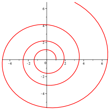
Figure 1. Logarithmic spiral $\gamma(t)$ (1.9) for $a=+5$, restricted to $t\geq 0$.

1.4.1. Loewner process for the logarithmic spiral

Let us define, as before, $\Omega_{t}:=\mathbb{C}\setminus\gamma[t,+\infty)$ and let $f_{t}:\mathbb{D}\rightarrow\Omega_{t}$ be the associated Riemann map, i.e., the conformal map such that

$$f_{t}(0)=0,f_{t}^{\prime}(0)>0.$$ (1.10)

By the Koebe distorsion theorem, $\lim_{t\rightarrow-\infty}f_{t}^{\prime}(0)=0$ and $\lim_{t\rightarrow+\infty}f_{t}^{\prime}(0)=+\infty$. Then, there exists $t_{0}$ such that $f_{t_{0}}^{\prime}(0)=1$. One also has that $f_{t_{0}}(e^{i\theta_{0}})=\gamma(t_{0})=e^{(1+ia)t_{0}}$ for some $\theta_{0}\in[0,2\pi).$ Consider now the function $\tilde{f}_{t}$ defined by

$$\tilde{f}_{t}(z):=e^{(1+ia)t}f_{t_{0}}(e^{-iat}z).$$

We have $\tilde{f}_{t}(0)=0,\tilde{f}_{t}^{\prime}(0)=e^{t},$ and

$$\tilde{f}_{t}(e^{i(\theta_{0}+at)})=e^{(1+ia)(t+t_{0})}=\gamma(t+t_{0}).$$ (1.11)

Hence from (1.11), $\tilde{f}_{t}:\mathbb{D}\rightarrow\Omega_{t+t_{0}}$ is the Loewner process corresponding to the curve

$$\tilde{\gamma}(t):=\gamma(t+t_{0}),\,\,t\in\mathbb{R},$$

with the associated driving function $\tilde{\lambda}(t):=e^{i(\theta_{0}+at)}$.

Define then the curve,

$$\eta(t):=e^{-i\theta_{0}}\tilde{\gamma}(t),\,\,\,t\in\mathbb{R},$$

and the conformal map,

$$h_{t}(z):=e^{-i\theta_{0}}\tilde{f}_{t}(e^{i\theta_{0}}z).$$

One still has $h_{t}(0)=0,h_{t}^{\prime}(0)=e^{t},$ and $h_{t}(e^{iat})=\eta(t)$, so that $h_{t}$ is the Loewner map corresponding to $\eta(t)$ and the associated process is driven by $\lambda(t):=e^{iat}$.
Notice that the curve $\eta$ is obtained by a time-translation and a rotation of the logarithmic spiral $\gamma$. Thus the integral means spectrum will be the same for the time zero Loewner maps $h_{0}$ and $\tilde{f}_{0}$.

1.4.2. Complex generalized spectrum for the complete logarithmic spiral

We first focus on the complete spiral, for which we first establish the following theorem.

Theorem 1.1.

The complex generalized integral means spectrum of the complete logarithmic spiral $\gamma(t)=e^{(1+ia)t},\,t\in\mathbb{R}$, is given, for $p,q\in\mathbb{C}$, by

$$\beta(p,q;a)=\sup\left\{0,\beta_{1}(p,q;0,a),\beta_{2}(p,q;0,a)\right\},$$ (1.12)

where

$$\begin{split}&\beta_{1}(p,q;0,a):=2\Re{\left(\frac{p-q}{1-ia}\right)}+\Re{p}-1,\\ &\beta_{2}(p,q;0,a):=-2\Re{\left(\frac{p-q}{1-ia}\right)}+\Re{p}-1.\end{split}$$ (1.13)

Proof.

Let us define on the unit disk $\mathbb{D}$, the Moebius map $\xi:z\mapsto\xi(z):=i\frac{1-z}{1+z}$, and consider the function $\Phi$ defined on $\mathbb{D}$ as,

$$\Phi(z):=\exp\left[\frac{2}{1-ia}\log\xi(z)\right]=\left(i\frac{1-z}{1+z}\right)^{\frac{2(1+ia)}{1+a^{2}}},\,\,\,z\in\mathbb{D}.$$

Define also the strip domain ${\mathbb{S}}_{\pi}:=\{x+iy:x\in\mathbb{R},\,\,0<y<\pi\}$. We know that $z\mapsto\xi(z)$ conformally maps $\mathbb{D}$ onto upper half-plane $\mathbb{H}$, while $z\mapsto\log(z)$ conformally maps $\mathbb{H}$ onto the strip ${\mathbb{S}}_{\pi}$. Lastly, $z\mapsto\exp\left(\frac{2}{1-ia}z\right)$ conformally maps the strip domain ${\mathbb{S}}_{\pi}$ onto $\mathbb{C}\setminus\gamma$, with a cut along the whole logarithmic spiral $\gamma:=\{\gamma(t)=e^{(1+ia)t},t\in{\mathbb{R}}\}$. Consequently, $\Phi$ is a conformal map from the unit disk $\mathbb{D}$ to the complement of the whole logarithmic spiral $\gamma$, with $\Phi(1)=0,\Phi(-1)=\infty$.

It enjoys the useful property,

$$\Phi^{\prime}(z)=\frac{2}{1-ia}\big{(}\log\xi(z)\big{)}^{\prime}\Phi(z)=-\frac{4}{1-ia}\frac{\Phi(z)}{1-z^{2}}.$$ (1.14)

Owing to (1.14),the complex mixed moments of $\Phi$ read

$$\frac{\Phi^{\prime}(z)^{p}}{\Phi(z)^{q}}=\left(-\frac{4}{1-ia}\frac{1}{1-z^{2}}\right)^{p}\,\frac{1}{\Phi(z)^{q-p}},$$ (1.15)

so that

$$\left|\frac{\Phi^{\prime}(z)^{p}}{\Phi(z)^{q}}\right|=\left|\left(-\frac{4}{1-ia}\right)^{p}\right|\times\frac{\left|\Phi(z)^{p-q}\right|}{\left|(1-z^{2})^{p}\right|}.$$ (1.16)

We have explicitly

$$\left|(1-z^{2})^{p}\right|=\left|1-z\right|^{\Re p}\left|1+z\right|^{\Re p}e^{-\Im p\,\arg(1-z^{2})},$$ (1.17)

and

$$\left|\Phi(z)^{p-q}\right|=\exp\Re\left[\frac{2(p-q)}{1-ia}\log\xi(z)\right].$$ (1.18)

Setting $b=b(p,q):=\frac{2(p-q)}{1-ia}$, we have $\Re\left[b\log\xi(z)\right]=\Re b\,\log|\xi(z)|-\Im b\,\Im\log\xi(z)$, and since $\log\xi(z)\in{\mathbb{S}}_{\pi}$, its imaginary part stays bounded. We thus have the following (logarithmic) equivalence near the two possible singular points $z=\pm 1$,

$$\left|\Phi(z)^{p-q}\right|\stackrel{{\scriptstyle\cdot}}{{\sim}}|\xi(z)|^{\Re b(p,q)}=\left|\frac{1-z}{1+z}\right|^{\Re\frac{2(p-q)}{1-ia}}.$$ (1.19)

Using (1.16), (1.17), and (1.19), we finally arrive at

$$\left|\frac{\Phi^{\prime}(z)^{p}}{\Phi(z)^{q}}\right|\stackrel{{\scriptstyle\cdot}}{{\sim}}\left|\frac{1-z}{1+z}\right|^{\Re\frac{2(p-q)}{1-ia}}\left|1-z\right|^{-\Re p}\left|1+z\right|^{-\Re p}.$$ (1.20)

Behaviour near infinity and near the origin. For $z=re^{i\theta}$ near $z=-1$ (point at $\infty$ on the spiral), $|1+z|^{2}=r^{2}+2r\cos\theta+1$ behaves like $(1-r)^{2}+(\pi-\theta)^{2}$. Similarly, near $z=+1$ (point $0$ on the spiral), $|1-z|^{2}$ behaves like $(1-r)^{2}+\theta^{2}$. The integral of (1.20) along the circle $|z|=r$ for $r\to 1^{-}$ is thus dominated near $z=-1$ by the contribution of the angular neighbourhood of $\theta=\pi$, while near $z=+1$ it is symmetrically dominated by that of the angular neighbourhood of $\theta=0$. From the explicit form of the integrand (1.20), we readily obtain the overall asymptotic behaviour as $r\to 1^{-}$ of the integral means,

$$\int_{r\partial\mathbb{D}}\left|\frac{\Phi^{\prime}(z)^{p}}{\Phi(z)^{q}}\right||dz|\stackrel{{\scriptstyle\cdot}}{{\sim}}\left(1-r\right)^{-\beta_{\Phi}(p,q;a)},\,\,\,r\to 1^{-},$$ (1.21)

where the integral means spectrum $\beta_{\Phi}$ is given by the largest exponent,

$$\beta_{\Phi}(p,q;a):=\beta_{1}(p,q;0,a)\vee\beta_{2}(p,q;0,a)\vee 0,$$ (1.22)

with the two dual spectra defined as,

$$\beta_{1}(p,q;0,a):=2\Re\frac{p-q}{1-ia}+\Re p-1,$$ (1.23)

$$\beta_{2}(p,q;0,a):=2\Re\frac{q-p}{1-ia}+\Re p-1.$$ (1.24)

∎

Remark 1.2.

Singularity localization. Exponent $\beta_{1}$ is associated with the singularity near $z=-1$ on $\mathbb{D}$ in (1.20), i.e., at infinity on the spiral, while $\beta_{2}$ corresponds to that near $z=+1$, i.e., near the tip at origin $0$, around which the spiral indefinitely winds.

Remark 1.3.

Conformal invariance by inversion and duality. The full logarithmic spiral is conformally invariant under the complex inversion, $z\mapsto 1/z$, since $1/\gamma(t)=\gamma(-t)$, and $t\in\mathbb{R}$. This inversion exchanges the roles of origin and infinity, and maps the interior of $\mathbb{D}$ to its exterior. The complex generalized integral means spectrum then obeys the duality property (1.1). Spectra (1.23) and (1.24) are indeed dual of each other under the corresponding exchange $q-p\mapsto p-q$, resulting in the expected invariance under duality of the integral means spectrum $\beta_{\Phi}$ (1.22) for the complete logarithmic spiral.

1.4.3. Complex generalized spectrum of the half spiral

Consider now $h_{0}(z)$, the conformal map corresponding to the whole-plane Loewner process driven by $e^{iat}$, stopped at time $t=0$, the image of which, $\gamma(t)=e^{(1+ia)t},\,t\geq 0$, we may call the half spiral (Fig. 1). The complex generalized integral means spectrum of the half logarithmic spiral is given by the following theorem. (See Fig. 2.)

Theorem 1.2.

The complex generalized integral means spectrum of $h_{0}$, where $h_{t}$ is the whole-plane Loewner process driven by $\lambda(t)=e^{iat}$, and whose trace is the half logarithmic spiral $\gamma(t)=e^{(1+ia)t},\,t\geq 0$, is given, for $p,q\in\mathbb{C}$, by

$$\beta(p,q;\kappa=0,a)=\sup\left\{-\Re{p}-1,0,\beta_{1}(p,q;0,a)=2\Re{\left(\frac{p-q}{1-ia}\right)}+\Re{p}-1\right\}.$$ (1.25)

From this, one immediately deduces the following corollary, which yields the real generalized integral means spectrum of the half spiral.

Corollary 1.1.

The real generalized integral means spectrum of $h_{0}$, where $h_{t}$ is the whole-plane Loewner process driven by $\lambda(t)=e^{iat}$, and whose trace is the half logarithmic spiral $\gamma(t)=e^{(1+ia)t},\,t\geq 0$, is given, for $p,q\in\mathbb{R}$, by

$$\beta(p,q;\kappa=0,a)=\sup\left\{-p-1,0,\beta_{1}(p,q;0,a)=2\frac{p-q}{1+a^{2}}+p-1\right\}.$$ (1.26)

This result for the real case, $p,q\in\mathbb{R}$, is illustrated in Fig. 2.

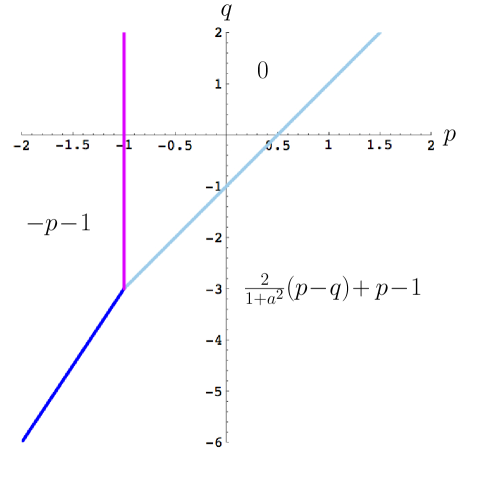
Figure 2. The three phases of the generalized integral means spectrum of the logarithmic spiral, with $\beta_{\mathrm{tip}}(p;\kappa=0)=-p-1$, $\beta_{0}(p;\kappa=0)=0$, $\beta_{1}(p,q;\kappa=0,a)=\frac{2}{1+a^{2}}(p-q)+p-1$ (Corollary 1.1).

Proof.

$\bullet$ Behaviour near infinity. For $t\geq 0$, the half spiral and whole spiral are identical, thus have the same spectrum near infinity. So we use the conformal map $\Phi$ to calculate the integral means spectrum near $\infty$, i.e., by considering the mixed moments (1.20) for $z\to-1$ only, as well as the corresponding contribution to integral (1.21). Because of Remark 1.2, the associated spectrum is $\beta_{1}$ (1.23).
$\bullet$ Behaviour near the tip. Let $\phi(z):=\frac{z}{(1-z)^{2}},z\in\mathbb{D}$, with $\phi(-1)=-\frac{1}{4},\phi(0)=0,\phi(1)=\infty$, be the Koebe function, conformally mapping the unit disk to the straight cut plane as $\mathbb{D}\mapsto\mathbb{C}\setminus(-\infty,-\frac{1}{4}]$. Let $g$ be the conformal map from $\mathbb{C}\setminus(-\infty,-\frac{1}{4}]$ to the plane cut by the half spiral, $\Omega_{0}:=\mathbb{C}\setminus\gamma[0,\infty)$, with $g(0)=0,g(-\frac{1}{4})=\gamma(0)=1$. Then $h_{0}=g\circ\phi$. Notice that both $g$ and $g^{\prime}$ are bounded near $\phi(-1)=-\frac{1}{4}$, hence also $h_{0}$ near $z=-1$. Let us define $r\partial\mathbb{D}_{\varepsilon}:=\{z:|z|=r,|1+z|<\varepsilon\}$, for some fixed $\varepsilon$ such that $1-r<\varepsilon<1$, as the neighbourhood along the circle $r\partial\mathbb{D}$ of the pre-image $z=-1$ by $h_{0}$ of the half spiral tip $\gamma(0)=1$. In this domain, we have the logarithmic equivalence, as $r\to 1^{-}$,

$$\int_{r\partial\mathbb{D}_{\varepsilon}}\left|\frac{h_{0}^{\prime}(z)^{p}}{h_{0}(z)^{q}}\right||dz|\stackrel{{\scriptstyle\cdot}}{{\sim}}\int_{r\partial\mathbb{D}_{\varepsilon}}|\phi^{\prime}(z)^{p}||dz|,\,\,\,r\to 1^{-}.$$

We thus obtain that the integral means spectrum near the tip of the half spiral is the same as the ims near the tip of the half line, which is simply,

$$\beta_{\mathrm{tip}}(p;\kappa=0):=-\Re p-1.$$ (1.27)

$\bullet$ Bulk behaviour. Away from $\infty$ and the tip, the half spiral is rectifiable, and its bulk integral means spectrum is trivial, $\beta_{0}(p;\kappa=0)=0$. This ends the proof of Theorem 1.2. ∎

2. Complex generalized spectrum of drifted whole-plane SLE

2.1. Introduction

In this section, we will predict the exact form of the generalized integral means spectrum $\beta_{1}(p,q;\kappa,a)$ associated with the whole-plane SLE_κ with drift $a$. As we shall see, its most symmetric and simplest form is obtained for the complex generalized spectrum where the exponents are complex variables $p,q\in\mathbb{C}$. We shall use a non-fully rigorous method inherited from theoretical physics. More specifically, we use two-dimensional quantum gravity where the Euclidean Lebesgue measure is replaced by the Liouville quantum measure. This allows us to compute multifractal exponents in Liouville quantum gravity (LQG) for $p\in\mathbb{C}$ in the $q=0$ case, and for any $a\in\mathbb{R}$. The conversion to the complex multifractal spectrum in the Euclidean plane is then obtained by using the celebrated Knizhnik-Polyakov-Zamolodchikov (KPZ) relation [KPZ88, DK89, Dav88, DS09, DS11a, RV11, DS11b, DMS21]. The final step to get the complex generalized spectrum for $q\neq 0$ is then obtained via the introduction of the packing spectrum,

$$s_{1}(p,q;\kappa,a):=\beta_{1}(p,q;\kappa,a)-\Re\,p+1,$$ (2.1)

together with the fact that it is a function of variable $p-q$ only.

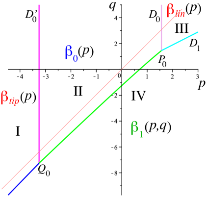
Figure 3. Phase transition lines for the generalized integral means spectrum of whole-plane SLE_κ with no drift $a=0$. The standard ims of the $q=2p$ exterior version crosses phases I, II, III only, while the $q=0$ standard ims of the interior version crosses phases I, II, IV (from Ref. [DHLZ18]).

2.2. Driftless and real case

Let us denote by $\beta(p,q;\kappa,a)$ the generalized integral means spectrum of the whole-plane SLE_κ with drift coefficient $a$. Ref. [DHLZ18] studied the $a=0$ case and for $(p,q)\in\mathbb{R}^{2}$, for which it is shown that $\beta(p,q;\kappa,a=0)$ has four possible forms, of which three are independent of $q$,

$$\beta_{\mathrm{tip}}(p;\kappa) := -p-1+\frac{1}{4}\left(4+\kappa-\sqrt{(4+\kappa)^{2}-8\kappa p}\right),$$ (2.2)

$$\beta_{0}(p;\kappa) := -p+\frac{4+\kappa}{4\kappa}\left(4+\kappa-\sqrt{(4+\kappa)^{2}-8\kappa p}\right),$$ (2.3)

$$\beta_{\mathrm{lin}}(p;\kappa) := p-\frac{(4+\kappa)^{2}}{16\kappa},$$ (2.4)

$$\beta_{1}(p,q;\kappa,a=0) := p+2(p-q)-\frac{1}{2}-\frac{1}{2}\sqrt{1+2\kappa(p-q)}.$$ (2.5)

The separatrices between the different phases are located as follows [DHLZ18, Theorem 1.7] (See Fig. 3.) For $p\leq-1-\frac{3\kappa}{8}$ there is a (quartic) curve ending at point $Q_{0}:p_{0}^{\prime}=-1-\frac{3\kappa}{8},q_{0}^{\prime}=-2-\frac{7\kappa}{8}$, that separates the half-plane into two parts, $\beta$ being equal to $\beta_{\mathrm{tip}}$ above that curve and to $\beta_{1}$ below it. In the strip $-1-\frac{3\kappa}{8}\leq p\leq\frac{3(4+\kappa)^{2}}{32\kappa}$, there is a section of parabola joining $Q_{0}$ to point $P_{0}=(p_{0},q_{0})$, with

$$p_{0}=\frac{3(4+\kappa)^{2}}{32\kappa},\,\,\,q_{0}=\frac{(4+\kappa)(8+\kappa)}{16\kappa},$$ (2.6)

that separates the strip into two parts, an upper one where $\beta=\beta_{0}$ and a lower one where $\beta=\beta_{1}$. Finally the half-plane $p\geq p_{0}$ is similarly split by the half-line with unit slope starting at $P_{0}$ into an upper part where $\beta=\beta_{\mathrm{lin}}$, while $\beta=\beta_{1}$ in the lower part. It should be noticed that the generalized spectrum $\beta$ is not everywhere the maximum of the four spectra listed above [DHLZ18].

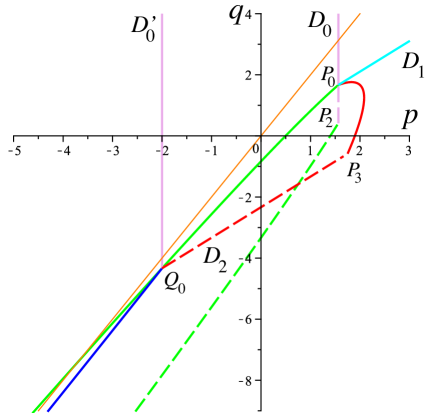
Figure 4. Domains of validity of the proofs in the driftless case $a=0$, $\kappa=8/3$ (from Ref. [DHLZ18]).

The existence of these phase transition lines was established in [DHLZ18] within a connected semi-infinite domain of the $(p,q)$ plane, as indicated in Fig. 4. This domain of validity sweeps the plane from its upper-left part up to a piecewise boundary first made, for increasing values of $p$, of the dotted green parabola up to its intersection with the straight line $D_{2}$ of equation $p-q=1+\frac{\kappa}{2}$. It then follows this line up to its intersection $P_{3}=\left(1+\frac{2}{\kappa},\frac{4-\kappa^{2}}{2\kappa}\right)$ with the red parabola. From there, the boundary is made of the section of red parabola up to point $P_{0}$ (2.6), followed by the straight line $D_{1}$ of equation $q-p=\frac{16-\kappa^{2}}{32\kappa}$. These restrictions to the domain of proof are due to technicalities involved in the proofs [DNNZ15, BDZ17, DHLZ18], and the spectrum is supposed to be still given by $\beta_{1}$ in the whole connected domain located to the right of the piecewise boundary just described. Recent work by Xuan Hieu Ho extends the domain of validity to the whole interior of the red parabola [Ho22]. Let us now turn to the complex generalized spectrum of whole-plane SLE for $(p,q)\in\mathbb{C}^{2}$, possibly with a drift term.

2.3. Complex case with drift

Claim 2.1.

For $p,q\in\mathbb{C}$, and $a=0$, the complex spectrum $\beta_{1}$ of whole-plane SLE can be obtained by combining Liouville quantum gravity and Coulomb gas methods. It is

$$\beta_{1}(p,q;\kappa,a=0)=s_{1}(p-q;\kappa,a=0)+\Re p-1$$ (2.7)

$$s_{1}(p-q;\kappa,a=0)=s_{1}(\tau):=2\tau+\frac{1}{2}-\frac{1}{2}\sqrt{1+2\kappa\tau},$$ (2.8)

$$1+2\kappa\tau:=\frac{1}{2}\left\{1+2\kappa\Re(p-q)+\left|1+2\kappa(p-q)\right|\right\}.$$ (2.9)

Claim 2.2.

For $a\neq 0$, the complex spectrum $\beta_{1}$ of whole-plane SLE with drift is given by an extension of the above proofs, as

$$\beta_{1}(p,q;\kappa,a)=s_{1}(p-q;\kappa,a)+\Re p-1$$ (2.10)

$$s_{1}(p-q;\kappa,a)=s_{1}(\tau):=2\tau+\frac{1}{2}-\frac{1}{2}\sqrt{1+2\kappa\tau},$$ (2.11)

$$1+2\kappa\tau:=\frac{1}{2}\left\{\Re\left[(1+ia)^{2}+2\kappa(p-q)\right]+\left|(1+ia)^{2}+2\kappa(p-q)\right|\right\}.$$ (2.12)

Remark 2.1.

In the limit $\kappa\to 0$, the integral means spectrum (1.23) of the half-spiral is recovered from (2.10) (2.11), by observing that the expansion to order $O(\kappa)$ of the r.h.s. of (2.12) indeed yields $\tau=\Re{\left(\frac{p-q}{1-ia}\right)}$.

As we shall see in Section 3.4, this complex spectrum yields the correct answer along an integrable complex parabola in the complex space $(p,q)\in\mathbb{C}^{2}$.

In the real moment case, $(p,q)\in\mathbb{R}^{2}$, the generalized integral means spectrum $\beta_{1}(p,q;\kappa,a)$ associated with whole-plane SLE_κ with drift $a$ is given by the explicit formulae:

$$\beta_{1}(p,q;\kappa,a)=p+2\tau-\frac{1}{2}-\frac{1}{2}\sqrt{1+2\kappa\tau},$$ (2.13)

$$1+2\kappa\tau:=\frac{1}{2}\left\{1-a^{2}+2\kappa(p-q)+\sqrt{\left[1-a^{2}+2\kappa(p-q)\right]^{2}+4a^{2}}\right\}.$$ (2.14)

Consequence 2.1.

Eq. (2.14) can be inverted into:

$$p-q=\tau\left(1+\frac{a^{2}}{1+2\kappa\tau}\right).$$ (2.15)

Therefore the phase transition lines in the $(p,p-q)$ plane for $a\neq 0$ are obtained from those for $a=0$ by the non-linear transform,

$$p\mapsto p,$$

$$p-q=\tau\mapsto p-q=\tau\left(1+\frac{a^{2}}{1+2\kappa\tau}\right).$$ (2.16)

In the work [DHLZ18], the location of the various phase transition lines in the case of whole-plane SLE without drift was established with the help of several master curves: a so-called ‘red parabola’ where the one-point function $G$ (1.6) is integrable, a so-called ‘green parabola’ where the spectrum changes from $\beta_{0}$ to $\beta_{1}$, and a ‘blue quartic’ where it changes from $\beta_{\mathrm{tip}}$ to $\beta_{1}$, as well as several straight lines, like $D_{0}^{\prime}$ where the spectrum changes from $\beta_{\mathrm{tip}}$ to $\beta_{0}$, $D_{0}$ where it changes from $\beta_{0}$ to $\beta_{\mathrm{lin}}$, and $D_{1}$ where it changes from $\beta_{\mathrm{lin}}$ to $\beta_{1}$ (Fig. 3). These curves are also instrumental in delimiting the domains of validity of the proofs (Fig. 4). Applying the non-linear transform (2.16) in the $(p,q-p)$ plane to these curves yields the corresponding curves in the case of whole-plane SLE with drift. They are illustrated in Figs. 5 and 6.

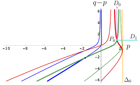
Figure 5. Non-linear mapping (2.16) of the red and green parabolae and blue quartic of Ref. [DHLZ18] (here $\kappa=2$, $a=1$).

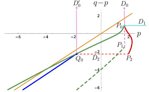
Figure 6. Non-linear mapping (2.16) of the domains of validity of the proofs, as shown in Fig. 4 from [DHLZ18] (here $\kappa=2$, $a=1$).

2.3.1. Phase diagram

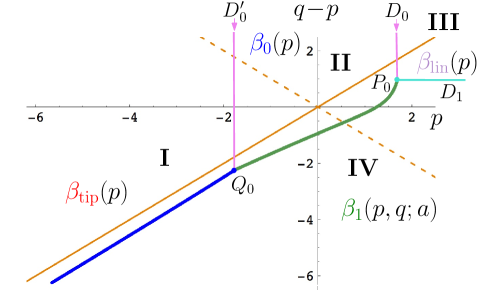
Figure 7. Phase transition lines for the generalized integral means spectrum of simple whole-plane SLE_κ with drift (here $\kappa=2$, $a=1$). The first bisector with $q=2p$ (orange continuous line) corresponds to the standard integral means spectrum (ims) for the exterior case which crosses only phases I, II and III, whereas the second bisector with $q=0$ (orange dotted line) yields the standard ims for the interior case, which does enter phase IV with the $\beta_{1}$ spectrum.

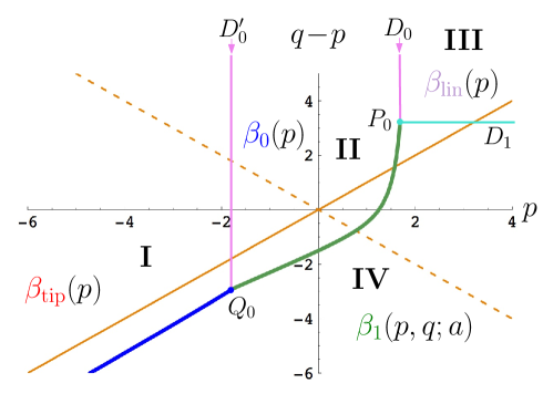
Figure 8. Phase transition lines for the generalized integral means spectrum of simple whole-plane SLE_κ with drift (here $\kappa=2$, $a=2$). The standard ims in the $q=2p$ exterior case crosses all four phases in the order I, II, IV and III, while the $q=0$ standard ims in the interior case crosses phases I, II and IV.

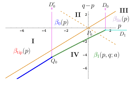
Figure 9. Phase transition lines for the generalized integral means spectrum of non-simple whole-plane SLE_κ with drift (here $\kappa=6$, $a=2$). The successive phase crossings of the two standard ims bisector lines are analogous to those depicted in Fig. 7.

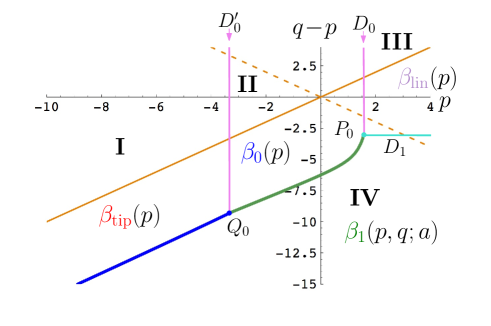
Figure 10. Phase transition lines for the generalized integral means spectrum of non-simple whole-plane SLE_κ with drift (here $\kappa=6$, $a=8$). The standard ims in the $q=2p$ exterior case crosses phases I, II, III only, while the $q=0$ standard ims in the interior case crosses all four phases in the order I, II, III and IV.

Various cases, relative to the values of parameters $\kappa$ and $a$, and drawn thanks to the non-linear mapping (2.16), are depicted in Figs. 7, 8, 9, and 10. In these figures, it is especially interesting to focus on the standard integral means spectra in the $p,q-p$ plane, obtained for the whole-plane exterior version, along the line $q=2p$, hence $q-p=p$ (first bisector, golden continuous line), and for the whole-plane interior version along the line $q=0$, hence $q-p=-p$ (second bisector, golden dotted line).

Point $P_{0}$ (2.6) in the drift-less case yields a value of $t_{0}:=p_{0}-q_{0}=\frac{\kappa^{2}-16}{32\kappa}$, so that $1+2\kappa t_{0}=\kappa^{2}/2$. The position of the translated point $P_{0}=(p_{0},\tilde{q}_{0})$ in the presence of drift $a$ is given by Eq. (2.16) as

$$\tilde{q}_{0}=p_{0}+\frac{16-\kappa^{2}}{32\kappa}\left(1+\frac{16a^{2}}{\kappa^{2}}\right).$$ (2.17)

To determine whether the first bisector enters region IV as in Fig. 8, so that the exterior standard whole-plane spectrum has a $\beta_{1}$ component, or avoids it as in Fig. 7, we need to know the sign of $\tilde{q}_{0}-2p_{0}$. If positive, the first bisector passes below $P_{0}$ so that it successively traverses regions I, II, IV and III as in Fig. 8. Owing to (2.6), this happens for

$$\frac{a^{2}}{\kappa^{2}}\geq a_{0}(\kappa):=\frac{1}{4}\frac{2+\kappa}{4-\kappa},\,\,\,\kappa<4.$$ (2.18)

This phenomenon thus occurs only for simple SLE_κ<4 curves, and for a sufficiently strong drift term $a$. Otherwise, one is in the configuration of Figs. 7, 9, and 10 for the first bisector, and the $\beta_{1}$ spectrum does not appear in the standard ims of the exterior whole-plane SLE with drift.

To determine whether the second bisector enters region III and crosses all four phases as in Fig. 10, so that the interior standard whole-plane spectrum has a linear component $\beta_{\mathrm{lin}}$, or whether it avoids the linear phase III as in Fig. 9, we need to know the position of $P_{0}$ with respect to that bisector, hence the sign of $\tilde{q}_{0}$. If negative, the second bisector passes above $P_{0}$, so that it successively traverses regions I, II, III and IV as in Fig. 10. This happens for

$$\frac{a^{2}}{\kappa^{2}}\geq\tilde{a}_{0}(\kappa):=\frac{1}{8}\frac{8+\kappa}{\kappa-4},\,\,\,\kappa>4.$$ (2.19)

This phenomenon thus occurs only for non-simple SLE_κ>4 curves, and for a sufficiently strong drift term $a$. Otherwise, one is in the configuration of Figs. 7, 8, and 9 for the second bisector, and the $\beta_{\mathrm{lin}}$ spectrum does not appear in the standard ims of the interior whole-plane SLE with drift, which takes the successive forms $\beta_{\mathrm{tip}},\beta_{0},\beta_{1}$.

Remark 2.2.

The two conditions on the reduced drift parameter, $a/\kappa\geq a_{0}(\kappa)$, in fact obey SLE duality [Dup00, Dup04, Dup06, Zha08, Dub09]. Defining the dual SLE parameter $\kappa^{\prime}=16/\kappa$, with $\kappa^{\prime}>4$ and $\kappa<4$, one checks that $\tilde{a}_{0}(\kappa^{\prime})=\tilde{a}_{0}(16/\kappa)=a_{0}(\kappa)$. The occurence here of this reduced drift parameter $a/\kappa$ may seem natural, if one recalls that the quadratic variation of $\sqrt{\kappa}B_{t}+at$ is $\kappa t$ and its mean $at$.

2.4. Derivation of Claims 2.1 and 2.2

2.4.1. Discourse on the Method

We are going to use here a Liouville quantum gravity (LQG) approach, which historically gave the first derivation of the standard SLE multifractal spectrum [Dup00], which was later confirmed by a standard mathematical approach [BS09, BDZ17, GMS18]. It is based on the celebrated Knizhnik-Polyakov-Zamolodchikov (KPZ) relation [KPZ88, Dav88, DK89] between scaling exponents in the Euclidean plane, and their counterparts under a random LQG measure that gives the scaling limit of the area measure on a random planar map. The KPZ relation is now mathematically proved [DS11a, RV11, DRSV14]. Although the LQG method, which originates in theoretical physics, is heuristic and not fully rigorous, it often offers the quickest and most natural path to the derivation of scaling exponents and multifractal spectra. It is also intimately related to the recently developed and rigorous wedge-welding theory in Liouville quantum gravity [She16, DMS21] (See in particular Appendix B in [DMS21] for a mathematically precise description of the KPZ interpretation.)

2.4.2. Derivation of Claim 2.1

Let us first recall that in the original work on whole-plane SLE [DNNZ15], the novel integral means spectrum, $\beta_{1}(p;\kappa):=\beta_{1}(p;q=0;\kappa,a=0)$, derived there for $p\in\mathbb{R}$, was related to some Liouville quantum gravity results obtained in [Dup04]. (See [DNNZ15, Section 1.3].) It was found that the related packing spectrum, defined as,

$$s_{1}(p;\kappa):=\beta_{1}(p;\kappa)-p+1,$$ (2.20)

is given by

$$s_{1}(p)=s_{1}(p;\kappa):=2p+\frac{1}{2}-\frac{1}{2}\sqrt{1+2\kappa p}.$$ (2.21)

When seen as a function of $p$, it has for inverse in terms of $s=s_{1}$,

$$p=\frac{s}{2}+\frac{\kappa}{8}{\mathcal{U}}^{-1}_{\kappa}(s),$$

where we defined

$${\mathcal{U}}^{-1}_{\kappa}(x):=\frac{1}{2\kappa}\left(\kappa-4+\sqrt{(4-\kappa)^{2}+16\kappa x}\right),$$

$${\mathcal{U}}_{\kappa}(x):=\frac{1}{4}x\left(\kappa x+4-\kappa\right),$$

$${\mathcal{V}}_{\kappa}(x):={\mathcal{U}}_{\kappa}\left(\frac{1}{2}\left(x+1-\frac{\kappa}{4}\right)\right)=\frac{1}{16\kappa}\left[\kappa^{2}x^{2}-(4-\kappa)^{2}\right].$$

Here ${\mathcal{U}}_{\kappa}$ is the KPZ function of Liouville quantum gravity adapted to SLE_κ, while ${\mathcal{V}}_{\kappa}$ is an associated function that relates boundary scaling dimensions to bulk ones [Dup04, Dup06]. Here we generalize methods introduced in [Dup00, DB02] and expounded in [Dup04, Dup06], and use notations similar to those of [Dup04], Section 8. For simplicity, we first implicitly assume SLE paths to be simple, i.e., with $\kappa\leq 4$, since the quantum gravity composition rules differ for the simple and non-simple phases of SLE [Dup04, Dup06]. Nevertheless, the results obtained also hold for $\kappa>4$. One has the set of identities,

$$p=x_{1}(s)-x_{1},$$ (2.22)

$$x_{1}(s):=2{\mathcal{V}}_{\kappa}\left[{\mathcal{U}}^{-1}_{\kappa}(s)+{\mathcal{U}}^{-1}_{\kappa}(\tilde{x}_{1})\right],$$ (2.23)

$$x_{1}:=x_{1}(0)=\frac{1}{8\kappa}(6-\kappa)(2-\kappa),$$ (2.24)

$$\tilde{x}_{1}:=\frac{6-\kappa}{2\kappa},\,\,\,{\mathcal{U}}^{-1}_{\kappa}(\tilde{x}_{1})=\frac{2}{\kappa}.$$ (2.25)

The scaling exponent $x_{1}(s)$ geometrically corresponds to a configuration where the SLE tip is locally avoiding a bunch of $s$ independent Brownian paths. The tip here should be understood as the so-called SLE ‘second tip’ at the origin [BDZ17], after inversion of unbounded (interior) whole-plane SLE [DNNZ15], as in Beliaev and Smirnov’s bounded (exterior) version of whole-plane SLE [BS09, BDZ17].

In the LQG approach, $s$ independent Brownian paths avoiding an SLE path near its tip are conformally equivalent to a certain number $k(s)$ of mutually-avoiding SLEs in a star configuration, given by

$$k(s)=1+\frac{{\mathcal{U}}^{-1}_{\kappa}(s)}{{\mathcal{U}}^{-1}_{\kappa}(\tilde{x}_{1})},$$ (2.26)

such that $x_{1}(s)=2{\mathcal{V}}_{\kappa}(2k(s)/\kappa)$. When $p\in\mathbb{C}$, its imaginary part $\tilde{t}:=\Im p$ corresponds to exponentially weighting by $\exp(\tilde{t}\arg\mathcal{C})$ the mutually-avoiding SLE-Brownian path configurations $\mathcal{C}$, with local winding angle $\arg\mathcal{C}$ around the tip. One can then show by Coulomb gas arguments [DB02, Dup04, DB08] that the new scaling exponent associated with the tip is

$$\hat{x}_{1}(s,\tilde{t}):=x_{1}(s)-\frac{\kappa}{2}\frac{\tilde{t}^{\,2}}{k^{2}(s)}.$$ (2.27)

The average logarithmic spiral rotation rate $a$ near the tip is then obtained by Legendre transformation as [DB02, Dup04],

$$a=\frac{\partial}{\partial\tilde{t}}\,\hat{x}_{1}(s,\tilde{t}).$$ (2.28)

On the other hand, the real part of $p$, $t:=\Re p$, is now given by the generalization of (2.22),

$$\Re p=t=\hat{x}_{1}(s,\tilde{t})-x_{1},$$ (2.29)

whereas the packing spectrum for complex $p$, $s=s_{1}(p;\kappa)=\beta_{1}(p;\kappa)-\Re p+1$, is still given by (2.21), but now in terms of the reduced variable $\tau$,

$$\tau:=x_{1}(s)-x_{1},$$ (2.30)

$$s=s_{1}(\tau)=2\tau+\frac{1}{2}-\frac{1}{2}\sqrt{1+2\kappa\tau}.$$ (2.31)

From Eqs. (2.23), (2.26), we find the simple identity [DB02, Dup04]

$$\frac{1}{2\kappa}{k^{2}(s)}=x_{1}(s)+b,\,\,\,b=\frac{(4-\kappa)^{2}}{8\kappa}.$$ (2.32)

We thus find for (2.27) the simple formula,

$$\hat{x}_{1}(s,\tilde{t})=x_{1}(s)-\frac{1}{4}\frac{{\tilde{t}}^{2}}{x_{1}(s)+b},$$ (2.33)

from which (2.29) gives,

$$t=\hat{x}_{1}(s,\tilde{t})-x_{1} =x_{1}(s)-x_{1}-\frac{1}{4}\frac{{\tilde{t}}^{2}}{x_{1}(s)-x_{1}+c}$$

$$=\tau-\frac{1}{4}\frac{{\tilde{t}}^{2}}{\tau+c},\,\,\,c:=b+x_{1}=\frac{1}{2\kappa}.$$ (2.34)

Eq. (2.34) is then inverted into

$$\tau=\frac{1}{2}\left(t-c\pm\sqrt{(t+c)^{2}+\tilde{t}^{2}}\right),$$ (2.35)

which can be recast as

$$1+2\kappa\tau=\frac{1}{2}(1+2\kappa t)\pm\frac{1}{2}\sqrt{(1+2\kappa t)^{2}+4\kappa^{2}\tilde{t}^{2}}.$$ (2.36)

For $\tilde{t}=0$, we have $\tau=t$, which selects the (+)-branch in (2.36), and recalling that $t=\Re p,\tilde{t}=\Im p$, we obtain

$$1+2\kappa\tau=\frac{1}{2}(1+2\kappa\Re p)+\frac{1}{2}\sqrt{(1+2\kappa\Re p)^{2}+4\kappa^{2}\Im p^{2}},$$ (2.37)

which is the announced complex formula (2.14) for $p\in\mathbb{C},q=0$. When $q\neq 0$, we invoke the general validity of the observation made in Ref. [DHLZ18] that the generalized packing spectrum, $s_{1}(p,q;\kappa,a=0)=\beta_{1}(p,q;\kappa,a=0)-\Re p+1$, solely depends on the reduced variable $p-q$, hence $s_{1}(p,q;\kappa,0)=s_{1}(p-q,0;\kappa,0)$. ∎

2.4.3. Derivation of Claim 2.2

When $a\neq 0$, we modify the above aproach as follows. In the absence of Brownian paths, $s=0$, (2.33) becomes, since $x_{1}(0)=x_{1}$,

$$\hat{x}_{1}(0,\tilde{t})=x_{1}(0)-\frac{1}{4}\frac{{\tilde{t}}^{2}}{x_{1}(0)+b}=x_{1}-\frac{\kappa}{2}{\tilde{t}}^{2}.$$ (2.38)

The spiral rotation rate $a$ then corresponds via (2.28) to a parameter $\tilde{t}_{0}$ such that,

$$a=-\kappa\tilde{t}_{0},\,\,\,\hat{x}_{1}(0,\tilde{t}_{0})=x_{1}-\frac{a^{2}}{2\kappa}.$$ (2.39)

Re-centering around the spiralling rate $a$, we define, instead of (2.33),

$$\widehat{x}_{1}(s,\tilde{t}):=x_{1}(s)-\frac{1}{4}\frac{{(\tilde{t}-\tilde{t}_{0})}^{2}}{x_{1}(s)+b},$$ (2.40)

and substitute to (2.29), (2.34)

$$t=\widehat{x}_{1}(s,\tilde{t})-\hat{x}_{1}(0,\tilde{t}_{0}) =x_{1}(s)-x_{1}+\frac{a^{2}}{2\kappa}-\frac{1}{4}\frac{{(\tilde{t}-\tilde{t}_{0})}^{2}}{x_{1}(s)-x_{1}+c}$$

$$=\tau+\frac{a^{2}}{2\kappa}-\frac{1}{4}\frac{{(\tilde{t}-\tilde{t}_{0})}^{2}}{\tau+c},\,\,\,c=\frac{1}{2\kappa},\,\,\,\tilde{t}_{0}=-\frac{a}{\kappa}.$$ (2.41)

Thus, instead of (2.35) we find

$$\tau=\frac{1}{2}\left(t-c-\frac{a^{2}}{2\kappa}\pm\sqrt{\left(t+c-\frac{a^{2}}{2\kappa}\right)^{2}+(\tilde{t}-\tilde{t}_{0})^{2}}\right).$$ (2.42)

By again selecting the $(+)$-branch, and recalling that $t=\Re p$, $\tilde{t}=\Im p$, this can finally be written as

$$1+2\kappa\tau =\frac{1}{2}(1-a^{2}+2\kappa t)+\frac{1}{2}\sqrt{(1-a^{2}+2\kappa t)^{2}+4(a+\kappa\tilde{t})^{2}},$$

$$=\frac{1}{2}\left\{\Re\left[(1+ia)^{2}+2\kappa p\right]+\left|(1+ia)^{2}+2\kappa p\right|\right\}.$$ (2.43)

This is the announced result (2.12) for $p\in\mathbb{C},q=0$. Again, for $q\neq 0$, we invoke the fact [DHLZ18] that the generalized packing spectrum, $s_{1}(p,q;\kappa,a)=\beta_{1}(p,q;\kappa,a)-\Re p+1$, solely depends on the reduced variable $p-q$. ∎

3. Integrable probability for drifted whole-plane SLE

In order to anticipate the next section, let us put the computations in a more general setting.

3.1. Some background on Lévy processes

Definition 3.1.

A Lévy process is a stochastic process $(L_{t})_{t\geq 0}$ such that

• $L_{0}=0$ (a.s);

• For any discrete ordered set $\left\{t_{i},\,i\in I_{n}:=\{0,\cdots,n\}\right\}$, such that $t_{0}=0$ and $0\leq t_{i}<t_{i+1},\,\forall i\in I_{n-1}$, the successive increments ,$L_{t_{i+1}}-L_{t_{i}},\,\,i\in I_{n-1}$, are all mutually independent;

• For any $0\leq s\leq t$, $L_{t}-L_{s}$ has the same law as $L_{t-s}$.

• $L_{t}$ is continuous in probability, $\lim_{t\to 0}\mathbb{P}(|L_{t}-L_{0}|>\varepsilon)=0,\,\,\,\forall\varepsilon>0$, which rules out fixed discontinuities of the path $t\mapsto L_{t}$.

Notice that Brownian motion is a special Lévy process, and a general difference with Brownian motion is that random jumps are allowed. The characteristic function of a Lévy process $L_{t}$ has the form

$$\mathbb{E}[e^{i\xi L_{t}}]=e^{-t\eta(\xi)},$$ (3.1)

where $\eta$, called the Lévy symbol, is a continuous complex function of $\xi\in{\mathbb{R}}$, satisfying $\eta(0)=0$ and $\eta(-\xi)=\overline{\eta(\xi)}$. If $\eta(-\xi)=\eta(\xi)$, $L_{t}$ is a symmetric Lévy process. For Brownian motion, the Lévy symbol is $\eta(\xi)=\frac{\xi^{2}}{2}$. More generally, the function

$$\eta(\xi)=\frac{|\xi|^{\alpha}}{2},\alpha\in(0,2],$$

is the Lévy symbol of the so-called $\alpha-$stable process.

3.2. Derivation of the PDE

The inner whole-plane Loewner process is defined as the solution of the ODE in $\mathbb{C}$

$$\begin{cases}\partial_{t}g_{t}(z)=g_{t}(z)\frac{g_{t}(z)+\lambda(t)}{g_{t}(z)-\lambda(t)},\,\,\,t\geq 0,\\ \lim\limits_{t\rightarrow+\infty}e^{t}g_{t}(z)=z,\,\,\,\,\forall z\in\mathbb{C},\end{cases}$$ (3.2)

with driving function $\lambda(t)=e^{iL_{t}}$ where $L_{t}$ is real-valued; $g_{t}$ is a conformal mapping from a simply connected domain $\Omega_{t}\subset\mathbb{C}$ onto $\mathbb{D}$, where $\Omega_{t}$ is defined as $\Omega_{t}:=\left\{z\in\mathbb{C}:\tau_{z}>t\right\}$, where

$$\tau_{z}:=\sup\left\{t\in\mathbb{R}:\inf_{s\leq t}|g_{s}(z)-\lambda(s)|>0\right\}.$$

Its inverse function $f_{t}:=g_{t}^{-1}$ obeys the PDE (1.1),

$$\begin{cases}\partial_{t}f_{t}(z)=zf_{t}^{\prime}(z)\frac{\lambda(t)+z}{\lambda(t)-z}\\ \lim\limits_{t\rightarrow+\infty}f_{t}(e^{-t}z)=z,\,\,\,\,\forall z\in\mathbb{D},\end{cases}$$ (3.3)

where $f_{t}$ is now a mapping from $\mathbb{D}$ to the domain $\Omega_{t}=\mathbb{C}\setminus K_{t}$, where the connected set $K_{t}$ is the hull of the Loewner process. In this section, we will assume $L_{t},t\geq 0$, to be a Lévy process. The (complex) average integral means spectrum of the conformal map $f=f_{0}$, where $f_{t}$ is defined by (3.3), describes the singular behavior of the expectation,

$$\mathbb{E}[|f^{\prime}(z)^{p}|]=\mathbb{E}\left[f^{\prime}(z)^{\frac{p}{2}}\overline{f^{\prime}(z)}^{\frac{\bar{p}}{2}}\right],\quad p\in\mathbb{C}.$$ (3.4)

Similarly to the method used in [DHLZ18], we shall consider the Lévy-Loewner evolution (LLE) two-point function for $z_{1},z_{2}\in\mathbb{D}$, defined as,

$$G(z_{1},\overline{z}_{2}):=\mathbb{E}\left[z_{1}^{\frac{q}{2}}\frac{f^{\prime}(z_{1})^{\frac{p}{2}}}{f(z_{1})^{\frac{q}{2}}}\overline{z}_{2}^{\frac{\bar{q}}{2}}\frac{\overline{f^{\prime}(z_{2})}^{\frac{\bar{p}}{2}}}{\overline{f(z_{2})}^{\frac{\bar{q}}{2}}}\right],\quad p,q\in\mathbb{C}.$$ (3.5)

The moment (3.4) is the value $G(z,\bar{z})$ at coinciding points $z_{1}=z_{2}=z$, for the case $q=\bar{q}=0$. Following essentially the same approach as was introduced in [RS05, BS09, BDZ17, DHLZ18], we aim at finding a partial differential equation satisfied by $G$.

Since $f_{t}$ obeys a PDE instead of an ODE, the use of Itô calculus is problematic. A way to overcome this difficulty [BS09] is to consider the ODE (3.2) for negative times, and then compare the reverse function $g_{-t}$ to the inverse $g_{t}^{-1}$. The details are as follows.

For any fixed $s\geq 0$, define the auxiliary function $g_{t}^{(s)}$ such that: $g_{t}^{(s)}(z)=e^{-t}z$ for $t>s$, while for $t\leq s$, $g_{t}^{(s)}$ is the solution to the differential equation (3.2) with the initial (continuity) condition $g_{s}^{(s)}(z)=e^{-s}z$,

$$\begin{cases}\partial_{t}g_{t}^{(s)}(z)=g_{t}^{(s)}(z)\frac{g_{t}^{(s)}(z)+\lambda(t)}{g_{t}^{(s)}(z)-\lambda(t)},\,\,\,t\geq 0,\\ g_{s}^{(s)}(z)=e^{-s}z.\end{cases}$$ (3.6)

The family of conformal maps $(g_{t}^{(s)}(z))_{t\geq 0}$ is illustrated in Fig.11.

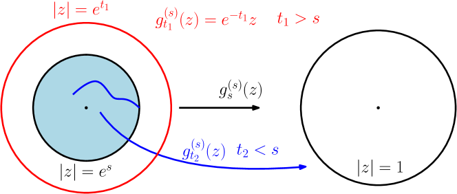
Figure 11. Family of auxiliary conformal maps $(g_{t}^{(s)})_{t\geq 0}$ for fixed $s\geq 0$. When $0\leq s\leq t$, $g_{t}^{(s)}(z)=e^{-t}z$ maps $e^{t}\mathbb{D}$ onto $\mathbb{D}$, whereas for $0\leq t\leq s$, $g_{t}^{(s)}(z)$ maps $e^{s}\mathbb{D}\setminus K_{t}$ onto $\mathbb{D}$.

Lemma 3.1.

With $g_{t}$ and $g_{t}^{(s)}$ defined as above, we have, for any $t\geq 0$,

$$\lim\limits_{s\rightarrow+\infty}g_{t}^{(s)}(z)=g_{t}(z).$$

This lemma is just the interior version of the following result by Lawler [Law05] for the exterior whole-plane case.

Lemma 3.2.

[Law05, Def. 6.28, Prop. 4.21] Let $\tilde{g}_{t}(z)$ be the solution of the differential equation,

$$\begin{cases}\partial_{t}\tilde{g}_{t}(z)=\tilde{g}_{t}(z)\frac{\tilde{\lambda}(t)+\tilde{g}_{t}(z)}{\tilde{\lambda}(t)-\tilde{g}_{t}(z)},\,\,\,t\leq 0,\\ \lim\limits_{t\rightarrow-\infty}e^{t}\tilde{g}_{t}(z)=z,\,\,\,\forall z\in\mathbb{C}\backslash\{0\}.\end{cases}$$ (3.7)

For any fixed $s\geq 0$, define $\tilde{g}_{t}^{(s)}(z)$ as: $\tilde{g}_{t}^{(s)}(z)=e^{-t}z$ if $t\leq-s$; for $t\geq-s$, $\tilde{g}_{t}^{(s)}(z)$ is the solution of the above differential equation with initial value $\tilde{g}_{-s}^{(s)}(z)=e^{s}z$. Then for $t\leq 0$, $\lim\limits_{s\rightarrow+\infty}\tilde{g}_{t}^{(s)}(z)=\tilde{g}_{t}(z)$.

In order to prove that Lemma 3.1 follows from 3.2, one applies complex inversion and time reversal so as to define for $t\leq 0$, $\tilde{g}_{t}^{(s)}(z):=1/g_{-t}^{(s)}(1/z)$ and $\tilde{\lambda}(t):=1/\lambda(-t)$, where $g_{t}^{(s)}(z)$ is defined by (3.6). Then $\tilde{g}_{t}^{(s)}$ is as in Lemma 3.2 and for $s\rightarrow+\infty$, it converges to the limit $\tilde{g}_{t}$ obeying (3.7). It then finally suffices to check that $g_{t}$, defined for $t\geq 0$ as $g_{t}(z):=1/{\tilde{g}_{-t}({1}/{z})}$, satisfies (3.2).

We then define a reversed radial LLE, as the solution to the ODE in the unit disk $\mathbb{D}$,

$$\partial_{t}\tilde{f}_{t}(z)=\tilde{f}_{t}(z)\frac{\tilde{f}_{t}(z)+\lambda(t)}{\tilde{f}_{t}(z)-\lambda(t)},\quad\tilde{f}_{0}(z)=z,\,\,\,\forall z\in\mathbb{D},\,\,\,t\geq 0.$$ (3.8)

Lemma 3.3.

For $f_{t}$ as defined in (3.3) and $\tilde{f}_{t}$ as defined in (3.8), we have the equivalence in law,

$$\lim_{t\rightarrow+\infty}e^{t}\tilde{f}_{t}(z)\stackrel{{\scriptstyle\rm(law)}}{{=}}f_{0}(z).$$ (3.9)

Proof.

For any fixed $s\geq 0$, let $g_{t}^{(s)}$ be as above. Then we have $g_{t}^{(s)}(z)\stackrel{{\scriptstyle\rm(law)}}{{=}}\tilde{f}_{t}\big{(}g_{0}^{(s)}(z)\big{)}$, because both obey (3.6), and they coincide at $t=0$ because of the initial condition in (3.8). We then have, $e^{t}\tilde{f}_{t}(z)\stackrel{{\scriptstyle\rm(law)}}{{=}}e^{t}g_{t}^{(s)}\big{(}(g_{0}^{(s)})^{-1}(z)\big{)}$. Letting $s=t$, we get

$$e^{t}\tilde{f}_{t}(z)\stackrel{{\scriptstyle\rm(law)}}{{=}}(g_{0}^{(t)})^{-1}(z),$$ (3.10)

and if we let $t\rightarrow+\infty$, by Lemma 3.1 we have $\lim\limits_{t\rightarrow+\infty}e^{t}\tilde{f}_{t}(z)\stackrel{{\scriptstyle\rm(law)}}{{=}}g_{0}^{-1}(z)=f_{0}(z)$. ∎

Let us define the auxiliary, time-dependent, radial variant of the LLE two-point function $G(z_{1},\bar{z}_{2})$ (3.5),

$$\widetilde{G}(z_{1},\bar{z}_{2},t) := \mathbb{E}\left[z_{1}^{\frac{q}{2}}\frac{\tilde{f}^{\prime}_{t}(z_{1})^{\frac{p}{2}}}{\tilde{f}_{t}(z_{1})^{\frac{q}{2}}}\overline{z}_{2}^{\frac{\bar{q}}{2}}\frac{\overline{\tilde{f}^{\prime}_{t}(z_{2})}^{\frac{\bar{p}}{2}}}{\overline{\tilde{f}_{t}(z_{2})}^{\frac{\bar{q}}{2}}}\right]$$

$$= \mathbb{E}\left[z_{1}^{\frac{q}{2}}X_{t}(z_{1})\overline{z}_{2}^{\frac{\bar{q}}{2}}Y_{t}(\bar{z}_{2})\right],$$ (3.11)

where $\tilde{f}_{t}$ is the reversed radial Loewner process (3.8), together with the shorthand notations,

$$X_{t}(z):=\frac{\tilde{f}^{\prime}_{t}(z)^{\frac{p}{2}}}{\tilde{f}_{t}(z)^{\frac{q}{2}}},\,\,\,Y_{t}(\bar{z}):=\overline{X_{t}(z)}=\frac{\overline{\tilde{f}^{\prime}_{t}(z)}^{\frac{\bar{p}}{2}}}{\overline{\tilde{f}_{t}(z)}^{\frac{\bar{q}}{2}}}.$$

By using (3.10), where the r.h.s. and its derivative are locally uniformly bounded by the Koebe distorsion theorem, the two-point function $G(z_{1},\bar{z}_{2})$ (3.5) is, by Lebesgue’s dominated convergence theorem, the limit

$$\lim_{t\rightarrow+\infty}e^{\Re(p-q)t}\widetilde{G}(z_{1},\bar{z}_{2},t)=G(z_{1},\bar{z}_{2}).$$ (3.12)

Remark 3.1.

The same argument implies that $\widetilde{G}(z_{1},\bar{z}_{2},t)$ and $G(z_{1},\bar{z}_{2})$ are holomorphic with respect to both $z_{1}$ and $\bar{z}_{2}$.

As explained in [RS05, BS09], the idea is then to construct a martingale $\mathcal{M}_{s}$ related to $\widetilde{G}$. The vanishing of the drift term in its Itô derivative then yields a partial differential equation obeyed by $\widetilde{G}$.

For $s\leq t$, define the two-point martingale $(\mathcal{M}_{s})_{t\geq s\geq 0}$ with

$$\mathcal{M}_{s}:=\mathbb{E}[X_{t}(z_{1})Y_{t}({\bar{z}}_{2})|\mathcal{F}_{s}],$$

where the random variable is integrable for fixed $z_{1}$ and $z_{2}$, and where $\mathcal{F}_{s}$ is the $\sigma$-algebra generated by the Lévy process filtration $\{L_{u},u\leq s\}$. By the Markov property of the Lévy process, we know that for any $s\leq t$,

$$\tilde{f}_{t}(z)\stackrel{{\scriptstyle\rm(law)}}{{=}}\lambda(s)\tilde{f}_{t-s}(\tilde{f}_{s}(z)/\lambda(s)).$$ (3.13)

Therefore,

$$\mathcal{M}_{s}=X_{s}(z_{1})Y_{s}(\bar{z}_{2})\widetilde{G}(z_{1,s},\bar{z}_{2,s};\tau),\,\,\,\tau:=t-s,\forall\tau>0,$$ (3.14)

where

$$z_{1,s}:=\frac{\tilde{f}_{s}(z_{1})}{\lambda(s)},\,\,\,\bar{z}_{2,s}:=\overline{\left(\frac{\tilde{f}_{s}(z_{2})}{\lambda(s)}\right)}=\overline{\tilde{f}_{s}(z_{2})}\lambda(s).$$

In order to prepare for Itô calculus, we have [DHLZ18, Section 4, Eqs. (47-49)]

$$dX_{s}(z_{1})= X_{s}(z_{1})\left[\frac{p}{2}-\frac{q}{2}-\frac{p}{(1-z_{1,s})^{2}}+\frac{q}{1-z_{1,s}}\right]ds,$$ (3.15)

$$dY_{s}(\bar{z}_{2})= Y_{s}(\bar{z}_{2})\left[\frac{\bar{p}}{2}-\frac{\bar{q}}{2}-\frac{\bar{p}}{(1-\bar{z}_{2,s})^{2}}+\frac{\bar{q}}{1-\bar{z}_{2,s}}\right]ds,$$ (3.16)

$$\frac{\partial z_{1,s}}{\partial s}{\big{|}_{\lambda(s)}}= z_{1s}\frac{z_{1,s}+1}{z_{1,s}-1},\,\,\,\frac{\partial\bar{z}_{2,s}}{\partial s}\big{|}_{\lambda(s)}=\bar{z}_{2,s}\frac{\bar{z}_{2,s}+1}{\bar{z}_{2,s}-1}.$$ (3.17)

Let us write $\mathcal{M}_{s}$ as a formal function of two variables,

$$H(s,L_{s}):=\mathcal{M}_{s}=X_{s}(z_{1})Y_{s}(\bar{z}_{2})\widetilde{G}(z_{1,s},\bar{z}_{2,s},t-s).$$

It is a (local) martingale for all $s\leq t$, thus by Itô calculus its total $s$-derivative vanishes,

$$\Lambda H(s,L_{s})+\partial_{s}H(s,L_{s})=0,$$

where $\Lambda$ is the generator of the Lévy process $L_{s}$.

We have from Eqs. (3.15), (3.16), (3.17),

$$\partial_{s}H=H\left[\frac{p}{2}-\frac{q}{2}-\frac{p}{(1-z_{1,s})^{2}}+\frac{q}{1-z_{1,s}}\right]$$

$$+ H\left[\frac{\bar{p}}{2}-\frac{\bar{q}}{2}-\frac{\bar{p}}{(1-\bar{z}_{2,s})^{2}}+\frac{\bar{q}}{1-\bar{z}_{2,s}}\right]$$

$$- X_{s}(z_{1})Y_{s}(\bar{z}_{2})\partial_{\tau}\widetilde{G}(z_{1,s},\bar{z}_{2,s},t-s)$$

$$+ X_{s}(z_{1})Y_{s}(\bar{z}_{2})\partial_{z_{1}}\widetilde{G}(z_{1,s},\bar{z}_{2,s},t-s)z_{1s}\frac{z_{1,s}+1}{z_{1,s}-1}$$

$$+ X_{s}(z_{1})Y_{s}(\bar{z}_{2})\partial_{\bar{z}_{2}}\widetilde{G}(z_{1,s},\bar{z}_{2,s},t-s)\bar{z}_{2,s}\frac{\bar{z}_{2,s}+1}{\bar{z}_{2,s}-1},$$

where $\tau:=t-s$. Since neither $X_{s}(z)$ nor its complex conjugate $Y_{s}(z)$ vanish in $\mathbb{D}$, we deduce that

$$-\Lambda\widetilde{G}(z_{1,s},\bar{z}_{2,s},t-s) =\widetilde{G}(z_{1,s},\bar{z}_{2,s},t-s)\left[\frac{p}{2}-\frac{q}{2}-\frac{p}{(1-z_{1,s})^{2}}+\frac{q}{1-z_{1,s}}\right]$$

$$+\widetilde{G}(z_{1,s},\bar{z}_{2,s},t-s)\left[\frac{\bar{p}}{2}-\frac{\bar{q}}{2}-\frac{\bar{p}}{(1-\bar{z}_{2,s})^{2}}+\frac{\bar{q}}{1-\bar{z}_{2,s}}\right]$$

$$-\partial_{\tau}\widetilde{G}(z_{1,s},\bar{z}_{2,s},t-s)+\partial_{z_{1}}\widetilde{G}(z_{1,s},\bar{z}_{2,s},t-s)z_{1s}\frac{z_{1,s}+1}{z_{1,s}-1}$$

$$+\partial_{\bar{z}_{2}}\widetilde{G}(z_{1,s},\bar{z}_{2,s},t-s)\bar{z}_{2,s}\frac{\bar{z}_{2,s}+1}{\bar{z}_{2,s}-1}.$$ (3.18)

Notice that by (3.12), it holds that, as $t\to+\infty$,

$$\Re(p-q)\exp\left[\Re(p-q)t\right]\widetilde{G}(z_{1},\bar{z}_{2},t)+\exp\left[\Re(p-q)t\right]\partial_{t}\widetilde{G}(z_{1},\bar{z}_{2},t)\to 0,$$

so that

$$\lim_{t\to+\infty}\exp\left[\Re(p-q)t\right]\partial_{t}\widetilde{G}(z_{1},\bar{z}_{2},t)=-\Re(p-q)\,G(z_{1},z_{2}).$$ (3.19)

Multiplying both sides of (3.2) by $\exp\left[\Re(p-q)(t-s)\right]$, and letting $t\to+\infty$, we get

$$-\Lambda G(z_{1},\bar{z}_{2}) =G(z_{1},\bar{z}_{2})\left[\frac{p}{2}-\frac{q}{2}-\frac{p}{(1-z_{1})^{2}}+\frac{q}{1-z_{1}}\right]$$

$$+G(z_{1},\bar{z}_{2})\left[\frac{\bar{p}}{2}-\frac{\bar{q}}{2}-\frac{\bar{p}}{(1-\bar{z}_{2})^{2}}+\frac{\bar{q}}{1-\bar{z}_{2}}\right]$$

$$+\Re(p-q)G\left(z_{1},\bar{z}_{2}\right)$$

$$+\partial_{z_{1}}G(z_{1},\bar{z}_{2})z_{1}\frac{z_{1}+1}{z_{1}-1}+\partial_{\bar{z}_{2}}G(z_{1},\bar{z}_{2})\bar{z}_{2}\frac{\bar{z}_{2}+1}{\bar{z}_{2}-1}.$$ (3.20)

We finally get that $G(z_{1},\bar{z}_{2})$ satisfies $\mathcal{P}(D)\,G(z_{1},\bar{z}_{2})=0$, where

$$\mathcal{P}(D) :=\Lambda+z_{1}\frac{z_{1}+1}{z_{1}-1}\partial_{z_{1}}+\bar{z}_{2}\frac{\bar{z}_{2}+1}{\bar{z}_{2}-1}\partial_{\bar{z}_{2}}+p-q+\bar{p}-\bar{q}$$

$$-\frac{p}{(1-z_{1})^{2}}+\frac{q}{1-z_{1}}-\frac{\bar{p}}{(1-\bar{z}_{2})^{2}}+\frac{\bar{q}}{1-\bar{z}_{2}}.$$ (3.21)

Recall the definition of $\Lambda$ acting on a $C^{\infty}(\mathbb{R}^{2})$ function $u$,

$$\Lambda u(x)=\lim\limits_{t\downarrow 0}\frac{1}{t}\left({\mathbb{E}}^{x}[u(L_{t})]-u(x)\right).$$

For $k,l\in\mathbb{Z}$, we have for $z=re^{i\theta}$,

$$\Lambda(z^{k}\bar{z}^{l}) =r^{k+l}\Lambda(e^{i\theta(k-l)})=r^{k+l}\lim\limits_{t\downarrow 0}\frac{1}{t}\left({\mathbb{E}}^{\theta}[e^{i(k-l)L_{t}}]-e^{i(k-l)\theta}\right)$$

$$=r^{k+l}\lim\limits_{t\downarrow 0}\frac{1}{t}(e^{-t\eta(k-l)}-1)\,e^{i(k-l)\theta}=-\eta(k-l)z^{k}\bar{z}^{l},$$ (3.22)

where $\eta$ is the Lévy symbol of $L_{t}$.

3.3. Drifted Brownian motion

In this section, we consider the special Lévy process $L_{t}=at+\sqrt{\kappa}B_{t}$, where $a\in{\mathbb{R}},\kappa\geq 0$ and $B_{t}$ is standard one-dimensional Brownian motion. These processes are the most general Lévy processes with a.s. continuous trajectories. By definition of the Lévy symbol

$${\bf E}[e^{i\xi L_{t}}]={\bf E}[e^{i\xi(at+\sqrt{\kappa}B_{t})}]=e^{ia\xi t-t\frac{\kappa}{2}\xi^{2}}=e^{-t\eta(\xi)}.$$

So

$$\eta(\xi)=\frac{\kappa}{2}\xi^{2}-ia\xi.$$

By (3.2), we have

$$\Lambda(z^{k}\bar{z}^{l})=-\eta(k-l)z^{k}\bar{z}^{l}=\left(-\frac{\kappa}{2}(k-l)^{2}+ia(k-l)\right)z^{k}\bar{z}^{l},$$

so that the Lévy generator in the Brownian drift case is explicitly

$$\Lambda=-\frac{\kappa}{2}(z\partial_{z}-\bar{z}\partial_{\bar{z}})^{2}+ia(z\partial_{z}-\bar{z}\partial_{\bar{z}}).$$

The operator in (3.2) thus becomes

$$\mathcal{P}(D)= -\frac{\kappa}{2}(z_{1}\partial_{z_{1}}-\bar{z}_{2}\partial_{\bar{z}_{2}})^{2}+z_{1}\left(\frac{z_{1}+1}{z_{1}-1}+ia\right)\partial_{z_{1}}$$

$$+ \bar{z}_{2}\left(\frac{\bar{z}_{2}+1}{\bar{z}_{2}-1}-ia\right)\partial_{\bar{z}_{2}}+p-q+\bar{p}-\bar{q}$$

$$- \frac{p}{(1-z_{1})^{2}}+\frac{q}{1-z_{1}}-\frac{\bar{p}}{(1-\bar{z}_{2})^{2}}+\frac{\bar{q}}{1-\bar{z}_{2}}.$$ (3.23)

3.3.1. Algebraic solutions

We want to find some solutions to the PDE

$$\mathcal{P}(D)G(z_{1},\bar{z}_{2})=0,\,\,\,G(0,0)=1,$$ (3.24)

and follow the method of Ref. [DNNZ15], by looking for solutions of the form,

$$G(z_{1},\bar{z}_{2})=(1-z_{1})^{\alpha}(1-\bar{z_{2}})^{\bar{\alpha}}P(z_{1}\bar{z}_{2}),\,\,\,P(0)=1.$$ (3.25)

The action of the partial differential operator $\mathcal{P}(D)$ (3.3) readily gives

$$\mathcal{P}(D)[(1-z_{1})^{\alpha}(1-\bar{z_{2}})^{\bar{\alpha}}P(z_{1}\bar{z}_{2})]$$

$$=z_{1}\bar{z}_{2}(1-z_{1})^{\alpha-1}(1-\bar{z}_{2})^{\bar{\alpha}-1}(\kappa\alpha\bar{\alpha}P(z_{1}\bar{z}_{2})+2(z_{1}\bar{z}_{2}-1)P^{\prime}(z_{1}\bar{z}_{2}))$$

$$+[\mathcal{P}(\partial)(1-z_{1})^{\alpha}](1-\bar{z}_{2})^{\bar{\alpha}}P(z_{1}\bar{z}_{2})+[\mathcal{P}(\bar{\partial})(1-\bar{z}_{2})^{\bar{\alpha}}](1-z_{1})^{\alpha}P(z_{1}\bar{z}_{2}),$$

where

$$\mathcal{P}(\partial) :=-\frac{\kappa}{2}(z_{1}\partial_{z_{1}})^{2}+\left(\frac{z_{1}+1}{z_{1}-1}+ia\right)z_{1}\partial_{z_{1}}+p-q+\frac{q}{1-z_{1}}-\frac{p}{(1-z_{1})^{2}},$$ (3.26)

$$\mathcal{P}(\bar{\partial}) :=-\frac{\kappa}{2}(\bar{z}_{2}\partial_{\bar{z}_{2}})^{2}+\left(\frac{\bar{z}_{2}+1}{\bar{z}_{2}-1}-ia\right)\bar{z}_{2}\partial_{\bar{z}_{2}}+\bar{p}-\bar{q}+\frac{\bar{q}}{1-\bar{z}_{2}}-\frac{\bar{p}}{(1-\bar{z}_{2})^{2}}.$$

Notice that as complex conjugates,

$$\forall z\in\mathbb{D},\,\,\,\mathcal{P}(\partial)(1-z)^{\alpha}=0\Leftrightarrow\mathcal{P}(\bar{\partial})(1-\bar{z})^{\bar{\alpha}}=0.$$

So if we have,

$$\mathcal{P}(\partial)(1-z_{1})^{\alpha}=0,$$ (3.27)

then equation (3.24) reduces for (3.25) to

$$\kappa\alpha\bar{\alpha}P(z_{1}\bar{z}_{2})+2(z_{1}\bar{z}_{2}-1)P^{\prime}(z_{1}\bar{z}_{2})=0,\,\,\,P(0)=1$$

$$\Leftrightarrow P(z_{1}\bar{z}_{2})=(1-z_{1}\bar{z}_{2})^{-\frac{\kappa}{2}\alpha\bar{\alpha}}.$$ (3.28)

Let us now look for $\alpha$ such that Eq. (3.27) is satisfied. A direct computation readily gives [DNNZ15],

$$\mathcal{P}(\partial)(1-z)^{\alpha}=(1-z)^{\alpha}A+(1-z)^{\alpha-1}B+(1-z)^{\alpha-2}C,$$

where

$$A :=-\frac{\kappa}{2}\alpha^{2}+(1+ia)\alpha+p-q,$$ (3.29)

$$B :=\kappa\alpha^{2}-\left(\frac{\kappa}{2}+3-ia\right)\alpha+q,$$ (3.30)

$$C :=-\frac{\kappa}{2}\alpha^{2}+\left(2+\frac{\kappa}{2}\right)\alpha-p.$$ (3.31)

Notice that $A+B+C=0$. For any $\alpha\in\mathbb{C}$, the choice of $p,q$ such that $B=0$ and $C=0$, yields a solution to (3.27), hence together with (3.28) a solution (3.25) to (3.24).

We thus get the identity for drifted SLE,

$$G(z_{1},\bar{z}_{2})=\mathbb{E}\left[z_{1}^{\frac{q}{2}}\frac{f^{\prime}(z_{1})^{\frac{p}{2}}}{f(z_{1})^{\frac{q}{2}}}\bar{z}_{2}^{\frac{\bar{q}}{2}}\frac{\overline{f^{\prime}(z_{2})}^{\frac{\bar{p}}{2}}}{\overline{f(z_{2})}^{\frac{\bar{q}}{2}}}\right]=(1-z_{1})^{\alpha}(1-\bar{z}_{2})^{\bar{\alpha}}(1-z_{1}\bar{z}_{2})^{-\frac{\kappa}{2}\alpha\bar{\alpha}},$$ (3.32)

where the quadratic equations $B=0$, $C=0$ yield $p$ and $q$ in terms of $\alpha\in\mathbb{C}$ under the parametric form,

$$p=-\frac{\kappa}{2}\alpha^{2}+\left(2+\frac{\kappa}{2}\right)\alpha,\quad\,\,\,\alpha\in\mathbb{C},$$ (3.33)

$$q=-\kappa\alpha^{2}+\left(\frac{\kappa}{2}+3-ia\right)\alpha.$$ (3.34)

These results generalize those found for real $p,q$ and $a=0$ in [DHLZ18]. The complex $p,q$ case, still for $a=0$, has been thoroughly studied in Ref. [Ho16]. These equations generalize in the complex $p,q$ case, hence in four-dimensional space, the so-called red parabola of the real $(p,q)$-plane described in [DHLZ18]. By remark 3.1, and [DNNZ15, Lemma 3.1] the space of holomorphic solutions in $z_{1}$, $\bar{z}_{2}$ to the linear PDE in (3.24) is one-dimensional. As a consequence, we have proven the following

Theorem 3.1.

Let $f(z)=f_{0}(z)$ where $f_{t}$ is the drifted whole-plane Loewner process driven by $\lambda(t)=e^{i(at+\sqrt{\kappa}B_{t})},a\in\mathbb{R}$. For $(p,q)\in\mathbb{C}^{2}$, let the complex ‘red parabola’ $\mathcal{R}$ be defined as the two-dimensional manifold,

$$p=-\frac{\kappa}{2}\alpha^{2}+\left(2+\frac{\kappa}{2}\right)\alpha,\quad\,\,\,q-p=-\frac{\kappa}{2}\alpha^{2}+(1-ia)\alpha,\quad\,\,\,\alpha\in\mathbb{C}.$$ (3.35)

For $(p,q)\in\mathcal{R},\,\,z_{1},z_{2}\in\mathbb{D}$, we identically have

$$G(z_{1},\bar{z}_{2})=\mathbb{E}\left[z_{1}^{\frac{q}{2}}\frac{f^{\prime}(z_{1})^{\frac{p}{2}}}{f(z_{1})^{\frac{q}{2}}}\bar{z}_{2}^{\frac{\bar{q}}{2}}\frac{\overline{f^{\prime}(z_{2})}^{\frac{\bar{p}}{2}}}{\overline{f(z_{2})}^{\frac{\bar{q}}{2}}}\right]=(1-z_{1})^{\alpha}(1-\bar{z}_{2})^{\bar{\alpha}}(1-z_{1}\bar{z}_{2})^{-\frac{\kappa}{2}\alpha\bar{\alpha}}.$$

In particular, for $z_{1}=z_{2}=z$,

$$G(z,\bar{z})=\mathbb{E}\left[\left|z^{q}\right|\left|\frac{f^{\prime}(z)^{p}}{f(z)^{q}}\right|\right]=(1-z)^{\alpha}(1-\bar{z})^{\bar{\alpha}}(1-z\bar{z})^{-\frac{\kappa}{2}\alpha\bar{\alpha}}.$$ (3.36)

Hence, in the case of the complex red parabola (3.33), (3.34), we find that the complex generalized bulk spectrum is simply given by

$$\beta(p,q;\kappa,a)=\frac{1}{2}\kappa|\alpha|^{2}.$$ (3.37)

Remark 3.2.

Tip spectrum. When $2\Re\alpha+1\leq 0$, the presence in (3.36) of the singular factor $|(1-z)^{\alpha}|^{2}$, besides that of the bulk singular one, brings in an extra singular contribution to the integral means near $z=1$. This yields the new complex generalized tip spectrum [BS09, BDZ17, DHLZ18] along the red parabola (3.35),

$$\beta(p,q;\kappa,a)=\frac{1}{2}\kappa|\alpha|^{2}-2\Re\alpha-1,\,\,\,2\Re\alpha\leq-1.$$ (3.38)

Let us now turn to the case of real points along the complex red parabola $\mathcal{R}$ (3.35).

Corollary 3.1.

Let $f(z)=f_{0}(z)$ where $f_{t}$ is the drifted whole-plane Loewner process driven by $\lambda(t)=e^{i(at+\sqrt{\kappa}B_{t})}$. If $p,q$ take the following values:

$$p=p(\kappa,a)=\frac{(4+\kappa)^{2}}{8\kappa}\left(1+\frac{4a^{2}}{(2+\kappa)^{2}}\right),\;q=q(\kappa,a)=\frac{4+\kappa}{2\kappa}\left(1+\frac{4a^{2}}{(2+\kappa)^{2}}\right);$$

then the generalized integral means spectrum $\beta(p,q)$ of $f$ is equal to $p$.

Proof.

Let us look for exponents $p,q\in\mathbb{R}$, as parameterized by (3.33) and (3.34), with $\alpha=\alpha_{1}+i\alpha_{2}$ and $\alpha_{1},\alpha_{2}\in\mathbb{R}$. The condition $\Im{p}=0$ gives

$$\alpha_{2}\left(-\kappa\alpha_{1}+2+\frac{\kappa}{2}\right)=0,$$

hence either $\alpha_{2}=0$ or $\alpha_{1}={(4+\kappa)}/{2\kappa}$. The condition $\Im{q}=0$ yields

$$2\kappa\alpha_{1}\alpha_{2}-\left(\frac{\kappa}{2}+3\right)\alpha_{2}+a\alpha_{1}=0.$$

So if $\alpha_{2}=0$, we have either $\alpha_{1}=0$ or $a=0$. The first case is trivial, while the second one is the driftless case studied in [DHLZ18]. So, assuming $a\neq 0$, we obtain

$$\alpha_{1}=\frac{4+\kappa}{2\kappa},\quad\alpha_{2}=-\frac{a(4+\kappa)}{\kappa(2+\kappa)},$$

and

$$\alpha=\frac{4+\kappa}{2\kappa}\left(1-i\frac{2a}{2+\kappa}\right),$$

which in turn gives

$$p =p(\kappa,a):=\frac{(4+\kappa)^{2}}{8\kappa}\left(1+\frac{4a^{2}}{(2+\kappa)^{2}}\right),$$ (3.39)

$$q =q(\kappa,a):=\frac{4+\kappa}{2\kappa}\left(1+\frac{4a^{2}}{(2+\kappa)^{2}}\right).$$ (3.40)

Notice the further identity $\frac{\kappa}{2}\alpha\bar{\alpha}=p$. So for these special real values of $p$ and $q$ we have

$$\mathbb{E}\left[|z|^{q}\frac{|f^{\prime}(z)|^{p}}{|f(z)|^{q}}\right]=\frac{|(1-z)^{\alpha}|^{2}}{(1-|z|^{2})^{\frac{\kappa|\alpha|^{2}}{2}}}.$$

Notice also that $\Re{\alpha}>0$, so that the singularity at $z=1$ does not contribute to the circle integral

$$\int_{|z|=r<1}\frac{|(1-z)^{\alpha}|^{2}}{(1-|z|^{2})^{\frac{\kappa|\alpha|^{2}}{2}}}|dz|\asymp_{r\to 1^{-}}(1-r)^{-\frac{\kappa|\alpha|^{2}}{2}}.$$

So in the case (3.39) (3.40) the averaged generalized spectrum is simply $\beta(p,q)=p$. ∎

3.4. Check of integral means spectra on the integrable complex ‘red parabola’

As in [DHLZ18, Section 5.2.1], we will find that along the ‘red parabola’ $\mathcal{R}$, a succession of explicit complex integral means spectra reproduces the result $\beta:=\kappa|\alpha|^{2}/2$ of Theorem 3.1. In addition to formulae (2.7), (2.9), (2.10), (2.12) for the complex generalized spectrum $\beta_{1}$ of (drifted) whole-plane SLE, we shall need the SLE complex bulk spectrum $\beta_{0}(p),p\in\mathbb{C}$, and some extensions of both $\beta_{0}$ and $\beta_{1}$ [DHLZ18, Section 5.1].

3.4.1. SLE complex bulk spectrum

The SLE complex bulk spectrum $\beta_{0}(p),p\in\mathbb{C}$, can be obtained from the results of [DB02, DB08], and reads [BD23],

$$\beta_{0}(p)=s_{0}(p)+\Re p-1,$$ (3.41)

$$s_{0}(p)=s_{0}(t,\tilde{t}),\,\,\,t:=\Re p,\,\,\,\tilde{t}:=\Im p,$$ (3.42)

where the expression for $s_{0}(t,\tilde{t})$ is

$$s_{0}(t,{\tilde{t}})=1+b^{\prime}-t+\sqrt{(b^{\prime}-t)^{2}+{\tilde{t}}^{2}}-(2b^{\prime})^{\frac{1}{2}}\left[b^{\prime}-t+\sqrt{(b^{\prime}-t)^{2}+{\tilde{t}}^{2}}\right]^{\frac{1}{2}},$$ (3.43)

$$s_{0}(t,{0})=1+2(b^{\prime}-t)-2\sqrt{b^{\prime}}\sqrt{b^{\prime}-t},\quad\,\,\,b^{\prime}:=\frac{(4+\kappa)^{2}}{8\kappa}.$$ (3.44)

By introducing the variables,

$$\tau_{0} := b^{\prime}-t,$$ (3.45)

$$\bar{\tau} := \frac{1}{2}\left[b^{\prime}-t+\sqrt{(b^{\prime}-t)^{2}+{\tilde{t}}^{2}}\right]=\frac{1}{2}\left(\tau_{0}+\sqrt{\tau_{0}^{2}+{\tilde{t}}^{2}}\right),$$ (3.46)

the function $s_{0}(t,\tilde{t})$ (3.43) can then be recast as a function of the single variable $\bar{\tau}$, as

$$s_{0}(t,{\tilde{t}}) = s(\bar{\tau}):=1+2\bar{\tau}-2\sqrt{b^{\prime}}\sqrt{\bar{\tau}},$$ (3.47)

$$s_{0}(t,{0}) = s(\tau_{0})=1+2{\tau_{0}}-2\sqrt{b^{\prime}}\sqrt{{\tau_{0}}}.$$

3.4.2. Extensions of complex spectra $\beta_{0}$ and $\beta_{1}$

As in Refs.[DNNZ15, DHLZ18] it is natural to define auxiliary pseudo-integral means spectra, which help in understanding phase transitions that are mediated by overlaps between various analytic expressions of the spectra. They are obtained by restoring the usual sign indeterminacy in front of square root operations [DNNZ15, Section 4.2], [DHLZ18, Section 5.1]. Let us define the auxiliary functions,

$$\beta^{\pm}_{0}(p) :=s^{\pm}_{0}(p)+\Re p-1,\,\,\,p\in\mathbb{C},$$ (3.48)

$$s^{\pm}_{0}(p) =s^{\pm}_{0}(t,\tilde{t})=s^{\pm}(\bar{\tau}):=1+2\bar{\tau}\pm 2\sqrt{b^{\prime}}\sqrt{\bar{\tau}},$$ (3.49)

$$\bar{\tau} =\frac{1}{2}\big{(}\Re(b^{\prime}-p)+|b^{\prime}-p|\big{)},\,\,\,\,\,\,\quad\quad b^{\prime}=\frac{(4+\kappa)^{2}}{8\kappa}\,\,\,$$

$$=\frac{1}{2}\left(b^{\prime}-t+\sqrt{(b^{\prime}-t)^{2}+{\tilde{t}}^{2}}\right),\,\,t:=\Re p,\,\,\tilde{t}:=\Im p,$$

such that the complex bulk integral means spectrum (3.41) is given by the $(-)$-branch, $\beta_{0}\equiv\beta_{0}^{-}$. Similarly, we define

$$\beta^{\pm}_{1}(p,q;\kappa,a):=s_{1}^{\pm}(p-q;\kappa,a)+\Re p-1,\,\,\,p,q\in\mathbb{C},$$ (3.50)

$$s_{1}^{\pm}(p-q;\kappa,a)=s_{1}^{\pm}(\tau):=2\tau+\frac{1}{2}\mp\frac{1}{2}\sqrt{1+2\kappa\tau},$$ (3.51)

$$1+2\kappa\tau=\frac{1}{2}\left\{\Re\left[(1+ia)^{2}+2\kappa(p-q)\right]+\left|(1+ia)^{2}+2\kappa(p-q)\right|\right\},$$ (3.52)

such that the complex generalized spectrum (2.10) associated with spiral whole-plane SLE is given by the $(+)$-branch, $\beta_{1}\equiv\beta_{1}^{+}$.

3.4.3. Complex spectra $\beta_{1}^{\pm}$ along $\mathcal{R}$

From parameterization (3.35), we first find the identity along the red parabola $\mathcal{R}$,

$$(1+ia)^{2}+2\kappa(p-q)=(1+ia-\kappa\alpha)^{2}.$$

Using the general identity,

$$\frac{1}{2}\left[\Re(z^{2})+|z^{2}|\right]=(\Re z)^{2},z\in\mathbb{C},$$ (3.53)

we find for (3.52),

$$1+2\kappa\tau=[\Re(1+ia-\kappa\alpha)]^{2}=(1-\kappa\Re\alpha)^{2},$$

so that $s_{1}^{\pm}$ (3.51) reads

$$s_{1}^{\pm}(\tau)=\frac{1}{\kappa}\left[(1-\kappa\Re\alpha)^{2}-1\right]+\frac{1}{2}\mp\frac{1}{2}|1-\kappa\Re\alpha|.$$

We simultaneously have from (3.35) and (3.53),

$$\Re p=-\frac{\kappa}{2}\Re(\alpha^{2})+\left(2+\frac{\kappa}{2}\right)\Re\alpha=\frac{\kappa}{2}|\alpha^{2}|-\kappa(\Re\alpha)^{2}+\left(2+\frac{\kappa}{2}\right)\Re\alpha.$$ (3.54)

Combining the last two equations gives

$$s_{1}^{\pm}(\tau)+\Re p-1=\frac{\kappa}{2}|\alpha^{2}|+\frac{\kappa}{2}\Re\alpha-\frac{1}{2}\mp\frac{1}{2}|1-\kappa\Re\alpha|.$$

Therefore, we get for (3.50) the branch-dependent identity,

$$\beta^{\pm}_{1}(p,q;\kappa,a)=s_{1}^{\pm}(\tau)+\Re p-1=\frac{\kappa}{2}|\alpha^{2}|,\,\,\,\kappa\Re\alpha\gtreqqless 1.$$ (3.55)

This shows that the result of Theorem 3.1 for spiral whole-plane SLE is recovered for $\Re\alpha\geq 1/\kappa$ by the ‘physical’ branch $\beta_{1}^{+}$ of the generalized complex spectrum, and for $\Re\alpha\leq 1/\kappa$ by its ‘unphysical’ branch $\beta_{1}^{-}$, in a way entirely similar to the real case studied in [DHLZ18, Section 5.2.1].

3.4.4. Complex spectra $\beta^{\pm}_{0}$ along $\mathcal{R}$

From parameterization (3.35) we first get the identity,

$$b^{\prime}-p=\frac{\kappa}{2}\left(\alpha-\frac{4+\kappa}{2\kappa}\right)^{2},$$

from which we deduce with the help of (3.53),

$$\bar{\tau}=\frac{1}{2}\big{(}\Re(b^{\prime}-p)+|b^{\prime}-p|\big{)}=\frac{\kappa}{2}\left(\Re\alpha-\frac{4+\kappa}{2\kappa}\right)^{2}.$$

This in turn gives

$$s_{0}^{\pm}(\bar{\tau})=1+\kappa\left(\Re\alpha-\frac{4+\kappa}{2\kappa}\right)^{2}\pm\left(2+\frac{\kappa}{2}\right)\left|\Re\alpha-\frac{4+\kappa}{2\kappa}\right|,$$

which, together with (3.54) yields

$$s^{\pm}_{0}(\bar{\tau})+\Re p-1=\frac{\kappa}{2}|\alpha^{2}|-\left(2+\frac{\kappa}{2}\right)\Re\alpha+\kappa\left(\frac{4+\kappa}{2\kappa}\right)^{2}\pm\left(2+\frac{\kappa}{2}\right)\left|\Re\alpha-\frac{4+\kappa}{2\kappa}\right|.$$

Thus we find the branch-dependent identity,

$$\beta^{\pm}_{0}(p;\kappa)=s_{0}^{\pm}(\bar{\tau})+\Re p-1=\frac{\kappa}{2}|\alpha^{2}|,\,\,\,\kappa\Re\alpha\gtreqqless 2+\frac{\kappa}{2}.$$ (3.56)

We thus see that the result of Theorem 3.1 for spiral whole-plane SLE is recovered for $\Re\alpha\leq 2/\kappa+1/2$ by the ‘physical’ branch $\beta_{0}^{-}$ of the standard complex spectrum, and for $\Re\alpha\geq 2/\kappa+1/2$ by its ‘unphysical’ branch $\beta_{0}^{+}$, in a way again similar to the real case studied in [DHLZ18, Section 5.2.1]. We thus arrive at

Proposition 3.1.

Along the red parabola $\mathcal{R}$ (3.35), the integral means spectrum of the drifted whole-plane SLE is successively given by

$$\beta^{-}_{0}(p;\kappa)=\beta^{-}_{1}(p,q;\kappa,a)=\frac{\kappa}{2}|\alpha^{2}|,\,\,\,\Re\alpha\in(-\infty,{1}/{\kappa}],$$

$$\beta^{-}_{0}(p;\kappa)=\beta^{+}_{1}(p,q;\kappa,a)=\frac{\kappa}{2}|\alpha^{2}|,\,\,\,\Re\alpha\in[1/\kappa,2/\kappa+1/2],$$

$$\beta^{+}_{0}(p;\kappa)=\beta^{+}_{1}(p,q;\kappa,a)=\frac{\kappa}{2}|\alpha^{2}|,\,\,\,\Re\alpha\in[2/\kappa+1/2,+\infty).$$

Remark 3.3.

The two ‘physical’ integral means spectra $\beta_{0}^{-}$ (3.41) and $\beta_{1}^{+}$ (2.10) overlap along the red parabola $\mathcal{R}$ (3.35) in the interval $\Re\alpha\in[1/\kappa,2/\kappa+1/2]$, a result which can be directly compared to [DHLZ18, Eqs. (93)-(95)]. The integral means spectrum is always given by one of those two ‘physical’ spectra, which coincides with the ’physical’ branch of the other spectrum in the preceding overlap interval, or with its ‘unphysical’ branch outside the said interval.

This corresponds to the presence of a two-dimensional “overlap ribbon” on the red parabola, where the complex generalized integral means spectrum takes both the $\beta_{0}^{-}$ and $\beta_{1}^{+}$ forms. In the 4-dimensional $(p,q)$ space, there exists a larger phase-transition manifold, that is defined by the single condition that these two spectra are equal. This three-dimensional manifold must intersect the above overlap ribbon on a certain phase-transition line. The study of such phase-transition manifolds is left to a future work.

4. General Lévy processes with special symbols

In this section, we generalize the results in [DHLZ18], [DNNZ15], [Lou12], [LY13],[LY14] and [LY19] to the generalized integral means spectrum: in other words, we investigate the values of $(p,q)$ for which the generalized integral means spectrum for Lévy-Loewner evolution has an exact form.

For this purpose, we assume in this section that $G(z,\bar{z})$ (3.5) may be written as

$$G(z,\bar{z})=(1-z)(1-\bar{z})h(z,\bar{z}),$$

where $h(z,\bar{z})$ is separately analytic with respect to $z$ and $\bar{z}$ and satisfies the boundary condition $h(0,0)=1$. By applying (3.2), we get

$$\Lambda\left[(1-z)(1-\bar{z})h\right]$$

$$+ \left[\bar{q}(1-z)-\bar{p}\frac{1-z}{1-\bar{z}}+q(1-\bar{z})-p\frac{1-\bar{z}}{1-z}+(\bar{p}-\bar{q}+p-q)(1-z)(1-\bar{z})\right]h$$

$$+\frac{1-z}{1-\bar{z}}\bar{z}(1+\bar{z})(h+(\bar{z}-1)\partial_{\bar{z}}h)+\frac{1-\bar{z}}{1-z}z(1+z)(h+(z-1)\partial_{z}h)=0$$

The coefficient of $h=h(z,\bar{z})$ in this equation is the sum of a polynomial in $z$, $\bar{z}$, and of the polar part,

$$\frac{1-\bar{z}}{1-z}\left[-p+z(1+z)\right]+\frac{1-z}{1-\bar{z}}\left[-\bar{p}+\bar{z}(1+\bar{z})\right].$$

The latter clearly becomes pole free, i.e., a polynomial in $z$, $\bar{z}$ if and only if $p=\bar{p}=2$, which we shall hereafter assume. Under this condition, the above equation becomes

$$\Lambda[(1-z)(1-\bar{z})h]+(z+1)(\bar{z}-1)z\partial_{z}h+(\bar{z}+1)(z-1)\bar{z}\partial_{\bar{z}}h\\ +\left[(z-1)(3-\bar{q})\bar{z}+(\bar{z}-1)(3-q)z\right]h=0.$$ (4.1)

Besides the restriction to $p=2$, we shall also assume that $q\in{\mathbb{R}}$ and that the Lévy process $L_{t}$ is symmetric. We then get

$$\Lambda[(1-z)(1-\bar{z})h]+(z+1)(\bar{z}-1)z\partial_{z}h+(\bar{z}+1)(z-1)\bar{z}\partial_{\bar{z}}h\\ +(3-q)(2z\bar{z}-z-\bar{z})h=0.$$ (4.2)

In order to analyze this equation, we use the Fourier expansion of $t\mapsto h(re^{it},re^{-it})$:

$$h(z,\bar{z})=\sum_{n=-\infty}^{+\infty}\theta_{n}(\xi)z^{n},\;\xi:=z\bar{z},\,z=re^{it}.$$ (4.3)

When replacing $h$ by this expansion in the equation, we get a recursion formula between the $\theta_{n}$’s for $n\in\mathbb{Z}$. More precisely, by writing that the $n$’th Fourier coefficient of the left side of (4.2) vanishes, we obtain for $n\in\mathbb{Z}$,

$$2\xi(\xi-1)\theta_{n}^{\prime}(\xi)-\Big{(}\eta_{n}+n+(\eta_{n}+2q-n-6)\xi\Big{)}\theta_{n}$$

$$+\xi\Big{(}\eta_{n}+n+q-2\Big{)}\theta_{n+1}(\xi)+(\eta_{n}-n+q-2)\theta_{n-1}(\xi)=0.$$ (4.4)

Note that the assumption that $L_{t}$ is symmetric implies that $h(z,\bar{z})$ is symmetric w.r.t. $z$ and $\bar{z}$, which translates into,

$$\theta_{-n}(\xi)=\xi^{n}\theta_{n}(\xi),$$ (4.5)

from which we may simply recast expansion (4.3) above as

$$h(z,\bar{z})=\theta_{0}(\xi)+\sum_{n=1}^{\infty}\theta_{n}(\xi)(z^{n}+\bar{z}^{n})=\theta_{0}(\xi)+\sum_{n=1}^{\infty}2\theta_{n}(\xi)r^{n}\cos{nt}.$$ (4.6)

Before continuing, let us recall that we are looking for the integral means, i.e., the angular integrals,

$$I(r)=\int_{0}^{2\pi}G(re^{it},re^{-it})dt,$$

that can be easily expressed in terms of $\theta_{j}$’s as

$$\frac{I(r)}{2\pi}=(1+r^{2})\theta_{0}(r^{2})-2r^{2}\theta_{1}(r^{2}),$$ (4.7)

so that we only need to compute $\theta_{0}$ and $\theta_{1}$. For later purposes, let us also mention that $\theta_{0}(0)=1$. We thus focus on the equations for $n=0$ and $n=1$ (recall that $\eta_{0}=0$ and that $\theta_{-1}(\xi)=\xi\theta_{1}(\xi)$),

$$(\xi-1)\theta_{0}^{\prime}(\xi)-(q-3)\theta_{0}(\xi)+(q-2)\theta_{1}(\xi)=0,$$ (4.8)

$$2\xi(\xi-1)\theta_{1}^{\prime}(\xi)-\left[\eta_{1}+1+(\eta_{1}+2q-7)\xi\right]\theta_{1}(\xi)+(\eta_{1}+q-1)\xi\theta_{2}(\xi)$$

$$+(\eta_{1}+q-3)\theta_{0}(\xi)=0.$$ (4.9)

There are two simple cases where we can explicitly compute $\theta_{0}$ and $\theta_{1}$.

1. The first case is when the coefficient of the $\theta_{0}$-term in the second equation vanishes, i.e., when

   $$\eta_{1}=3-q,$$ (4.10)

   which requires $q<3$. In this case we may take $\theta_{1}=0$ (and actually $\theta_{n}=0$ for $n\geq 1$) and $\theta_{0}$ to be the solution to

   $$(\xi-1)\theta_{0}^{\prime}(\xi)-(q-3)\theta_{0}(\xi)=0,\;\theta_{0}(0)=1.$$

   This gives

   $$h(z,\bar{z})=\theta_{0}(\xi)=\frac{1}{(1-\xi)^{3-q}},$$ (4.11)

   and

   $$G(z,\bar{z})=\frac{(1-z)(1-\bar{z})}{(1-z\bar{z})^{3-q}},$$

   so that $\beta(2,q)=3-q>0$.

2. The second case is by letting the coefficient of the $\theta_{2}$-term vanish in the second equation, i.e., by taking

   $$\eta_{1}=1-q,$$ (4.12)

   which requires $q\leq 1$. We then get a system of coupled ODEs for $\theta_{0}$ and $\theta_{1}$, which we must solve with initial data $\theta_{0}(0)=1$, $\theta_{1}(0)$ finite. We find

   $$\begin{cases}\theta_{0}(\xi)=(1+\xi)(1-\xi)^{-(4-q)}\\[11.38109pt] \theta_{1}(\xi)=-\frac{2}{2-q}(1-\xi)^{-(4-q)},\end{cases}$$ (4.13)

   from which we deduce that $\beta(2,q)=4-q(>3)$.

Eqs. (4.11) and (4.13) generalize results of Ref. [LY14] to $q\neq 0$.

As noticed in [LY19], the preceding method generalizes: more precisely for any $n\geq 1$, if we let the coefficient of the $\theta_{n-1}$-term vanish in the $n$th equation, i.e., by taking $\eta_{n}=2-q+n$, then the solution of the system is $\theta_{p}=0$ for $p\geq n$, while $\theta_{0},..\theta_{n-1}$ are the solutions of the $n$ first equations, with the initial data $\theta_{0}(0)=1$.
Another possible generalization is by letting vanish, again in the $n$th equation, the coefficient of the $\theta_{n+1}$-term, i.e., by taking $\eta_{n}=2-q-n$; then the $n$ first equations allow us to compute $\theta_{0},..\theta_{n-1}$, which is more than needed since we only need to know $\theta_{0}$ and $\theta_{1}$. Having dealt in the last section with the $n=1$ case, let us now investigate the $n=2$ case.

4.1. The $\eta_{2}=4-q$ case

We take $\theta_{n\geq 2}=0$, and have to solve the following system of differential equations:

$$\begin{cases}(x-1)\theta_{0}^{\prime}(x)+(3-q)\theta_{0}(x)+(q-2)\theta_{1}(x)=0\\ 2x(x-1)\theta_{1}^{\prime}(x)-\left[1+\eta_{1}+(\eta_{1}+2q-7)x\right]\theta_{1}(x)+(\eta_{1}-3+q)\theta_{0}(x)=0.\end{cases}$$

We can assume the existence of a real number $\delta$ (to be determined later) and of two functions $f_{0},f_{1}:\,[0,1]\to{\mathbb{R}}$ such that $\theta_{0}$ and $\theta_{1}$ have the following form,

$$\theta_{0}(x)=(1-x)^{-\delta}f_{0}(x),\quad\theta_{1}(x)=(1-x)^{-\delta}f_{1}(x).$$

The ODE system satisfied by $f_{0}$ and $f_{1}$ is then

$$\begin{cases}(x-1)f_{0}^{\prime}+(3-q-\delta)f_{0}+(q-2)f_{1}=0\\ 2x(x-1)f_{1}^{\prime}-\left[1+\eta_{1}+(\eta_{1}+2q-7+2\delta)x\right]f_{1}+(\eta_{1}-3+q)f_{0}=0.\end{cases}$$ (4.14)

The form of the equation coefficients suggests we define $\delta^{\prime}$ as,

$$\delta^{\prime}:=\delta+q-3,$$ (4.15)

so that

$$\begin{cases}(x-1)f_{0}^{\prime}-\delta^{\prime}f_{0}+(q-2)f_{1}=0\\ 2x(x-1)f_{1}^{\prime}-\big{(}1+\eta_{1}+(\eta_{1}-1+2\delta^{\prime})x\big{)}f_{1}+(\eta_{1}-3+q)f_{0}=0.\end{cases}$$ (4.16)

From the first equation we extract $f_{1}$ as a function of $f_{0}$ and $f_{0}^{\prime}$ for $q\neq 2$,

$$f_{1}(x)=\frac{x-1}{2-q}f_{0}^{\prime}(x)-\frac{\delta^{\prime}}{2-q}f_{0}(x),\quad q\neq 2.$$ (4.17)

Substituting into (4.16), we obtain the following degree two differential equation satisfied by $f_{0}$,

$$\frac{2x(x-1)^{2}}{2-q}f_{0}^{\prime\prime}(x)+\left(2x(x-1)\frac{1-\delta^{\prime}}{2-q}-\frac{x-1}{2-q}\left(1+\eta_{1}+(\eta_{1}-1+2\delta^{\prime})x\right)\right)f_{0}^{\prime}(x)+$$

$$\left(\eta_{1}+q-3+\frac{\delta^{\prime}}{2-q}\left(1+\eta_{1}+(\eta_{1}-1+2\delta^{\prime})x\right)\right)f_{0}(x)=0.$$ (4.18)

We want to find $\delta^{\prime}$ such that this equation reads

$$x(x-1)f_{0}^{\prime\prime}(x)+((a+b+1)x-c)f_{0}^{\prime}(x)+abf_{0}(x)=0,$$ (4.19)

so that $f_{0}(x)=\,_{2}F_{1}(a,b,c;x)$, the hypergeometric function. This identification shows that $\delta^{\prime}$ must obey the following relation,

$$E(\delta^{\prime},\eta_{1},q):=2\delta^{\prime}(\delta^{\prime}+\eta_{1})+(2-q)(\eta_{1}+q-3)=0,$$ (4.20)

so that (4.1) simplifies into

$$x(x-1)f_{0}^{\prime\prime}(x)+\left(\frac{3-\eta_{1}-4\delta^{\prime}}{2}x-\frac{1+\eta_{1}}{2}\right)f_{0}^{\prime}(x)$$ (4.21)

$$-\delta^{\prime}\,\frac{1-\eta_{1}-2\delta^{\prime}}{2}f_{0}(x)=0.$$ (4.22)

This yields

$$a=-\delta^{\prime},\quad b=\frac{1-\eta_{1}}{2}-\delta^{\prime},\quad c=\frac{1+\eta_{1}}{2},$$ (4.23)

and we can choose $f_{0}(x)=\operatorname{{\vphantom{\mathnormal{F}}}_{2}\kern-0.5pt\mathnormal{F}_{1}}(a,b;c;x)$ and $\theta_{0}(x)=(1-x)^{-\delta}\operatorname{{\vphantom{\mathnormal{F}}}_{2}\kern-0.5pt\mathnormal{F}_{1}}(a,b;c;x)$. The other independent solution to the hypergeometric equation is

$$x^{1-c}\operatorname{{\vphantom{\mathnormal{F}}}_{2}\kern-0.5pt\mathnormal{F}_{1}}(1+a-c,1+b-c;2-c;x),$$

which is non-analytic at the origin $x=0$, hence is discarded as a candidate for $f_{0}$.

Before continuing, let us consider general symmetric Lévy processes: what are the possible couples $(\eta_{1},\eta_{2})$? We know that we must have $\eta_{2}\geq 0$ and the Lévy-Khinchine formula implies that $\eta_{1}\geq\eta_{2}/4$. It happens that every couple $(\eta_{1},\eta_{2})$ such that $\eta_{1}\geq\eta_{2}/4\geq 0$ actually corresponds to some (symmetric) Lévy process [App09] . Moreover the case $\eta_{1}=\eta_{2}/4$ exactly corresponds to an SLE process, while in the case $\eta_{2}=0$, $L_{t}$ is a pure jump process with jumps equal to $k\pi$, $k$ odd (notice that the other case is similar with $k$ even, yielding a continuous process on the circle).

For $\eta_{2}=4-q$, the preceeding constraints on $(\eta_{1},\eta_{2})$ become $q\leq 4$ and $\eta_{1}\geq\eta_{2}/4=1-q/4$, with equality for SLE_κ, with $\kappa=2-q/2$. Let us then define

$$D_{4-q}:=\{(q,\eta_{1})\in{\mathbb{R}}^{2};\,q\leq 4,\,\eta_{1}\geq 1-q/4\}.$$ (4.24)

Let us return to Eq. (4.20). It can be shown (see below) that $\eta_{1}^{2}-2(2-q)(\eta_{1}+q-3)\geq 0$ in $D_{4-q}$; we may thus extract $\delta^{\prime}$ from (4.20):

$$\delta_{\pm} =\delta^{\prime}_{\pm}+3-q$$

$$\delta^{\prime}_{\pm} =\delta^{\prime}_{\pm}(q,\eta_{1}):=\frac{1}{2}\left(-\eta_{1}\pm\sqrt{\eta_{1}^{2}-2(2-q)(\eta_{1}+q-3)}\right).$$ (4.25)

Replacing in (4.23) $\delta^{\prime}$ by its value in terms of $\eta_{1},q$, we get:

$$a_{\pm}=a_{\pm}(\eta_{1},q):=\frac{1}{2}\eta_{1}\mp\frac{1}{2}\sqrt{\eta_{1}^{2}-2(2-q)(\eta_{1}+q-3)}$$ (4.26)

$$b_{\pm}=b_{\pm}(\eta_{1},q):=\frac{1}{2}\mp\frac{1}{2}\sqrt{\eta_{1}^{2}-2(2-q)(\eta_{1}+q-3)}$$ (4.27)

$$c=c(\eta_{1},q):=\frac{1+\eta_{1}}{2}.$$ (4.28)

We can now compute $f_{1}$ as,

$$f_{1}(x) =\frac{x-1}{2-q}f_{0}^{\prime}(x)+\frac{-\delta^{\prime}}{2-q}f_{0}(x)$$

$$=\frac{a}{2-q}\operatorname{{\vphantom{\mathnormal{F}}}_{2}\kern-0.5pt\mathnormal{F}_{1}}(a,b;c;x)+\frac{ab(x-1)}{c(2-q)}\operatorname{{\vphantom{\mathnormal{F}}}_{2}\kern-0.5pt\mathnormal{F}_{1}}(a+1,b+1;c+1;x).$$ (4.29)

Using expression (4.7) for the integral means, we get

$$\frac{1}{2\pi}I(r)=(1-r^{2})^{-\delta}\left[(1+r^{2})f_{0}(r^{2})-2r^{2}f_{1}(r^{2})\right].$$ (4.30)

4.1.1. The $(+)$-branch

Let us first consider the case where

$$a=a_{+},\,b=b_{+}.$$

We then have $c-a_{+}-b_{+}=\sqrt{{\eta_{1}^{2}-2(2-q)(\eta_{1}+q-3)}}>0$, so that

$$0<\operatorname{{\vphantom{\mathnormal{F}}}_{2}\kern-0.5pt\mathnormal{F}_{1}}(a,b;c;1)=\frac{\Gamma(c)\Gamma(c-a-b)}{\Gamma(c-a)\Gamma(c-b)}<\infty.$$ (4.31)

If furthermore, $a+b+1<c$, then $\operatorname{{\vphantom{\mathnormal{F}}}_{2}\kern-0.5pt\mathnormal{F}_{1}}(a+1,b+1;c+1;1)<\infty$, and

$$\Delta:=\lim_{r\rightarrow 1}\left((1+r^{2})f_{0}(r^{2})-2r^{2}f_{1}(r^{2})\right)=2\left(1-\frac{a}{2-q}\right)\operatorname{{\vphantom{\mathnormal{F}}}_{2}\kern-0.5pt\mathnormal{F}_{1}}(a,b;c;1)<\infty.$$

We have thus proven that if $\Delta>0$, the spectrum is

$$\beta(2,q)=3-q+\delta_{+}^{\prime}(\eta_{1},q)=3-q+\frac{1}{2}\left(\sqrt{\eta_{1}^{2}-2(2-q)(\eta_{1}+q-3)}-\eta_{1}\right).$$

One can check that the coefficient $A:=1-a_{+}/(2-q)>0$ for $q<3$, whereas for $q\geq 3$, it vanishes for $\eta_{1}=1-q$ or $\eta_{1}=3-q$. In $D_{4-q}$, $A$ is thus positive since $\eta_{1}\geq 1-q/4$ is located outside the non-positive interval $[1-q,3-q]$. So we get that the spectrum is equal to $\delta_{+}$ on the subset of $D_{4-q}$ of points for which $a+b+1<c$. This condition is just $Z>1$, with

$$Z=Z(\eta_{1},q):={\eta_{1}^{2}-2(2-q)(\eta_{1}+q-3)}.$$ (4.32)

Note that $Z$ can be written as

$$Z =(q-3)^{2}+(\eta_{1}+q-2)^{2}-1$$ (4.33)

$$=X^{2}+Y^{2}-1,\quad X:=q-3,\quad Y:=\eta_{1}+q-2,$$ (4.34)

so that the condition $Z>1$ corresponds to the exterior of the blue ellipse of equation $Z=1$, i.e., $X^{2}+Y^{2}=2$ in the $(q,\eta_{1})$-plane (Fig. 12).

Notice that the set $Z=0$ is the co-centered green ellipse of equation $X^{2}+Y^{2}=1$, which only intersects $D_{4-q}$ at the tangency point $(\frac{12}{5},\frac{2}{5})$ with the $(\eta_{1}=1-q/4)$-line, implying that $Z\geq 0$ in $D_{4-q}$, as mentioned above.

In the interior of the blue ellipse, we instead have $a+b<c<a+b+1$, and we use the Euler transformation,

$$\operatorname{{\vphantom{\mathnormal{F}}}_{2}\kern-0.5pt\mathnormal{F}_{1}}(a,b;c;x)=(1-x)^{c-a-b}\operatorname{{\vphantom{\mathnormal{F}}}_{2}\kern-0.5pt\mathnormal{F}_{1}}(c-a,c-b;c;x),$$ (4.35)

so that

$$\operatorname{{\vphantom{\mathnormal{F}}}_{2}\kern-0.5pt\mathnormal{F}_{1}}(a+1,b+1;c+1;x)=(1-x)^{c-a-b-1}\operatorname{{\vphantom{\mathnormal{F}}}_{2}\kern-0.5pt\mathnormal{F}_{1}}(c-a,c-b;c+1;x).$$ (4.36)

We then get from (4.29)

$$f_{1}(x)=\frac{a}{2-q}\operatorname{{\vphantom{\mathnormal{F}}}_{2}\kern-0.5pt\mathnormal{F}_{1}}(a,b;c;x)-\frac{ab}{c}\frac{1}{(2-q)}(1-x)^{c-a-b}\operatorname{{\vphantom{\mathnormal{F}}}_{2}\kern-0.5pt\mathnormal{F}_{1}}(c-a,c-b;c+1;x).$$ (4.37)

We now have $\operatorname{{\vphantom{\mathnormal{F}}}_{2}\kern-0.5pt\mathnormal{F}_{1}}(a,b;c;1)<\infty$ and $\operatorname{{\vphantom{\mathnormal{F}}}_{2}\kern-0.5pt\mathnormal{F}_{1}}(c-a,c-b;c+1;1)<\infty$, so the second term in (4.37) still vanishes as $x\to 1$. This again yields

$$0<\Delta=2\left(1-\frac{a}{2-q}\right)\operatorname{{\vphantom{\mathnormal{F}}}_{2}\kern-0.5pt\mathnormal{F}_{1}}(a,b;c;1)<\infty,$$

i.e., the same result as found outside the blue ellipse. We thus find for the $(+)$-branch,

$$\frac{1}{2\pi}I(r)\sim 2(1-r^{2})^{-\delta_{+}}\left[1-\frac{a_{+}}{2-q}\right]\frac{\Gamma(c)\Gamma(c-a_{+}-b_{+})}{\Gamma(c-a_{+})\Gamma(c-b_{+})},\quad r\to 1^{-},\quad q\neq 2.$$ (4.38)

4.1.2. The $(-)$-branch

Let us now consider the other possible choice,

$$a=a_{-},\,b=b_{-}.$$

We then use both (4.35) and (4.36) in (4.29),

$$f_{1}(x)=(1-x)^{c-a-b}\left[\frac{a}{2-q}\operatorname{{\vphantom{\mathnormal{F}}}_{2}\kern-0.5pt\mathnormal{F}_{1}}(c-a,c-b;c;x)-\frac{ab}{c}\frac{1}{(2-q)}\operatorname{{\vphantom{\mathnormal{F}}}_{2}\kern-0.5pt\mathnormal{F}_{1}}(c-a,c-b;c+1;x)\right],$$ (4.39)

where now $c-a-b<0$, and where

$$\operatorname{{\vphantom{\mathnormal{F}}}_{2}\kern-0.5pt\mathnormal{F}_{1}}(c-a,c-b;c;1)=\frac{\Gamma(c)\Gamma(a+b-c)}{\Gamma(a)\Gamma(b)}<\infty,$$

$$\operatorname{{\vphantom{\mathnormal{F}}}_{2}\kern-0.5pt\mathnormal{F}_{1}}(c-a,c-b;c+1;1)=\frac{\Gamma(c+1)\Gamma(a+b-c+1)}{\Gamma(a+1)\Gamma(b+1)}<\infty.$$

From the well-known identity $\Gamma(x+1)=x\Gamma(x)$, we finally get for (4.39)

$$f_{1}(x)=(1-x)^{c-a-b}\frac{c-b}{2-q}\frac{\Gamma(c)\Gamma(a+b-c)}{\Gamma(a)\Gamma(b)}.$$

$I(r)$ (4.30) is now equivalent for $r^{2}=x\to 1$ to

$$\frac{1}{2\pi}I(r)\sim 2(1-x)^{-\delta_{-}+c-a-b}\left[1-\frac{c-b}{2-q}\right]\frac{\Gamma(c)\Gamma(a+b-c)}{\Gamma(a)\Gamma(b)}.$$

where we recall that $a=a_{-},b=b_{-}$. We now use the duality formulae

$$c-a_{-}=b_{+},\,\,c-b_{-}=a_{+},\,\,a_{-}+b_{-}-c=c-a_{+}-b_{+},$$

and

$$\delta_{\pm}=3-q+\delta^{\prime}_{\pm},\,\,\delta^{\prime}_{-}-\delta^{\prime}_{+}=c-a_{-}-b_{-},$$

so that for $r\to 1^{-}$,

$$\frac{1}{2\pi}I(r)\sim 2(1-r^{2})^{-\delta_{+}}\left[1-\frac{a_{+}}{2-q}\right]\frac{\Gamma(c)\Gamma(c-a_{+}-b_{+})}{\Gamma(c-a_{+})\Gamma(c-b_{+})},$$

which is exactly the same as the result (4.38) for the $(+)$-choice in Section 4.1.1.

Remark 4.1.

The $q=2$ case. Up to now, we have assumed that $q\neq 2$. The solution for $q=2$, thus $\eta_{2}=2,\eta_{1}\geq 1/2$, can be obtained by continuity as the $q\to 2$ limit of $f_{0}$ and $f_{1}$ (4.17). Eq. (4.26) gives

$$a_{+}=\frac{1}{2\eta_{1}}(\eta_{1}-1)(q-2)+\mathcal{O}\left((q-2)^{2}\right),$$

$$b_{+}=\frac{1}{2}(1-\eta_{1})+\mathcal{O}(q-2),\quad c=\frac{1}{2}(1+\eta_{1}),$$

so that $f_{0}=1$, and (4.17) has a finite limit when $q\to 2$,

$$f_{1}(x)=\frac{\eta_{1}-1}{2\eta_{1}}\left[1-\frac{1-\eta_{1}}{1+\eta_{1}}(1-x)\operatorname{{\vphantom{\mathnormal{F}}}_{2}\kern-0.5pt\mathnormal{F}_{1}}(1,\tfrac{1}{2}(3-\eta_{1});\tfrac{1}{2}(3+\eta_{1});x)\right],$$ (4.40)

together with $\delta^{\prime}_{+}=0$ and $\delta_{+}=1$. Eq. (4.38) simply becomes $\frac{1}{2\pi}I(r)\sim(1-r^{2})^{-1}\left(3-1/\eta_{1}\right)$, as $r\to 1^{-}$, so that $\beta(p=2,q=2)=1$.

We therefore proved the following

Theorem 4.1.

For a Lévy process, with symbols $\eta_{2}=4-q,\,\,\eta_{1}\geq\eta_{2}/4$ for $q\leq 4$, the generalized integral means spectrum of the corresponding LLE is

$$\beta(2,q)=3-q+\frac{1}{2}\left(\sqrt{\eta_{1}^{2}-2(2-q)(\eta_{1}+q-3)}-\eta_{1}\right).$$ (4.41)

In particular, if $q=2,\eta_{2}=2$, the standard integral means spectrum at $p=2$ of the logarithm of the LLE is independent of $\eta_{1}\geq 1/2$, and equal to $\beta(2,2)=1$.

In the $q=0$ case, Eq. (4.41) recovers a result of [LY19].

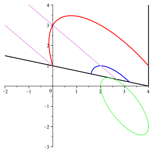
Figure 12. Domain lines in the $(q,\eta_{1})$ plane, for the $\eta_{2}=4-q$ case. The two purple straight lines have for equations, $\eta_{1}=1-q$ and $\eta_{1}=3-q$. The green, blue and red ellipses have for respective equations $X^{2}+Y^{2}=1,2,10$, with $X=q-3,Y=\eta_{1}+q-2$, with same center located at $(q,\eta_{1})=(3,-1)$.

4.1.3. Algebraic solutions

As a transition to the next section, let us look for purely algebraic solutions of the form,

$$\theta_{j}(x)=(1-x)^{-\alpha}f_{j}(x),\quad f_{j}(x)=A_{j}^{0}+A_{j}^{1}(1-x),\,j=0,1.$$

where $A_{j}^{k},k=0,1$ are fixed coefficients and with the understanding that $\theta_{j}=0$ for $j\geq 2$. Recall that the hypergeometric function $\operatorname{{\vphantom{\mathnormal{F}}}_{2}\kern-0.5pt\mathnormal{F}_{1}}$ is given by the well-known series expansion,

$$\operatorname{{\vphantom{\mathnormal{F}}}_{2}\kern-0.5pt\mathnormal{F}_{1}}(a,b;c;x)=\sum_{n=0}^{\infty}\frac{(a)_{n}(b)_{n}}{(c)_{n}}\frac{x^{n}}{n!}=1+\frac{ab}{c}\frac{x}{1!}+\frac{a(a+1)b(b+1)}{c(c+1)}\frac{x^{2}}{2!}+\cdots,$$ (4.42)

with

$$(a)_{n}=\begin{cases}1\quad\quad\quad\quad\quad\quad\quad\quad\quad\quad\,\,n=0\\ a(a+1)\cdots(a+n-1)\quad n\geq 1,\end{cases}$$

so that the fact that $f_{0}(x)=\operatorname{{\vphantom{\mathnormal{F}}}_{2}\kern-0.5pt\mathnormal{F}_{1}}(a,b;c;x)$ is at most linear in $x$ implies that either: $a=a_{+}=0$; $a_{+}=-1$; $b=b_{+}=0$; or $b_{+}=-1$. The function $f_{1}$ (4.17) is then also linear, assuming for now that $q\neq 2$. For later convenience, let us write (4.26) (4.27) as

$$a_{+}=\tfrac{1}{2}\eta_{1}-\tfrac{1}{2}{Z}^{1/2},\quad b_{+}=\tfrac{1}{2}-\tfrac{1}{2}{Z}^{1/2},$$ (4.43)

$$Z=\eta_{1}^{2}-2(2-q)(\eta_{1}+q-3).$$

$\bullet$ The $a_{+}=0$ case. The equation $Z=\eta_{1}^{2}$ gives for $q\neq 2$, $\eta_{1}=3-q$, which recovers the algebraic solutions, Eqs. (4.10) and (4.11). For $q=2$, Remark (4.1) and Eq. (4.40) yield for $\eta_{1}=1$, $f_{0}=1,f_{1}=0$, in agreement with (4.11).

$\bullet$ The $a_{+}=-1$ case. The equation $Z=(\eta_{1}+2)^{2}$ yields $(4-q)(\eta_{1}+q-1)=0$. Hence we first recover the algebraic case $\eta_{1}=1-q$, as in Eqs. (4.12) and (4.13). The other case, $q=4$, is the vertical boundary line for $D_{4-q}$ (Fig 12), where $\eta_{2}=0$, and for which Eq. (4.41) gives $\delta_{+}=\beta(p=2,q=4)=0$, so that $\theta_{j}=f_{j},\,j=0,1$. One further finds $b_{+}=-c=-\frac{1}{2}(1+\eta_{1})$, so that one gets the polynomial solutions, $f_{0}(x)=\operatorname{{\vphantom{\mathnormal{F}}}_{2}\kern-0.5pt\mathnormal{F}_{1}}(-1,b_{+};c;x)=1+x$, and from (4.17) $f_{1}(x)=\frac{1}{2}(1+x)$.

$\bullet$ The $b_{+}=0$ case. From (4.43) we get the condition $Z=1$, which in parameterization (4.33) of $Z$ (4.32) is just that defining the blue ellipse as $X^{2}+Y^{2}=2$. Its solution is given by $\eta_{1}=2-q\pm\sqrt{-q^{2}+6q-7}$. The condition $(q,\eta_{1})\in D_{4-q}$ (4.24) selects the $(+)$-branch only, and restricts the range of parameter $q$ to $q\in[\frac{8}{5},\frac{16}{5}]$ (see Fig. 12). This yields a first line of algebraic solutions,

$$\begin{cases}\eta_{1}&=2-q+\sqrt{1+(q-2)(4-q)}\\ \beta(2,q)&=\frac{1}{2}\left(5-q-\sqrt{1+(q-2)(4-q})\right)\\ q&\in[\frac{8}{5},\frac{16}{5}].\end{cases}$$

$\bullet$ The $b_{+}=-1$ case. From (4.43) we get the condition $Z=9$, which in parameterization (4.33) is defining a red ellipse as $X^{2}+Y^{2}=10$. Its solution is given by $\eta_{1}=2-q\pm\sqrt{1+6q-q^{2}}$. The condition $(q,\eta_{1})\in D_{4-q}$ (4.24) allows for both $(\pm)$-branches, but restricts the range of parameter $q$ to $[3-\sqrt{10},4]$ for the $(+)$-branch, and to $[3-\sqrt{10},0]$ for the $(-)$-branch (see Fig. 12). This finally gives algebraic solutions for,

$$\begin{cases}\eta_{1}&=2-q+\sqrt{1+6q-q^{2}}\\ \beta(2,q)&=\frac{1}{2}(7-q-\sqrt{1+6q-q^{2}})\\ q&\in[3-\sqrt{10},4],\end{cases}$$

and

$$\begin{cases}\eta_{1}&=2-q-\sqrt{1+6q-q^{2}}\\ \beta(2,q)&=\frac{1}{2}(7-q+\sqrt{1+6q-q^{2}})\\ q&\in[3-\sqrt{10},0].\end{cases}$$

From (4.42) and for $n\geq 2$, one further finds a whole series of algebraic solutions where the $f_{j}$’s are polynomials of degree $n$, when either $(a)_{n+1}=0$ or $(b)_{n+1}=0$, i.e., either $a_{+}=-n$ or $b_{+}=-n$.

$\bullet$ The $a_{+}=-n$ case. From (4.43), one finds

$$\eta_{1}=\frac{(2-q)(3-q)-2n^{2}}{2-q+2n}.$$ (4.44)

One recovers the two linear cases seen above, $n=0$, $\eta_{1}=3-q$ with $q\leq 8/3$ and $n=1$, $\eta_{1}=1-q$ with $q\leq 0$. For $n\geq 2$, the Lévy symbol condition $\eta_{1}\geq 1-q/4$ requires that $q\leq 2-2n$. Eq. (4.44) can be recast as

$$(2-q+2n)(\eta_{1}+q-3+2n)=2n(n-1).$$

This corresponds to a branch of a hyperbola $\mathcal{H}_{n}$ in the $(q,\eta_{1})$ plane, defined in affine coordinates by

$$X_{n}Y_{n}=2n(n-1),\,\,\,X_{n}:=2-q+2n,\,\,Y_{n}:=\eta_{1}+q-3+2n,\,\,\,q\leq 2-2n,\,\,n\geq 2.$$ (4.45)

$\bullet$ The $b_{+}=-n$ case. From (4.43) one readily finds

$$Z=(2n+1)^{2},$$ (4.46)

which in parameterization (4.33) is defining the ellipse $\mathcal{E}_{n}$ by the equation

$$X^{2}+Y^{2}=1+(2n+1)^{2}.$$

This in turn yields

$$\eta_{1}=2-q\pm\sqrt{(2-q)(q-4)+(2n+1)^{2}},$$ (4.47)

together with

$$\beta(2,q) =3-q+\frac{1}{2}\left(2n+1-\eta_{1}\right)$$ (4.48)

$$=\frac{1}{2}\left(2n+5-q\mp\sqrt{(2-q)(q-4)+(2n+1)^{2}}\right).$$

The condition $(q,\eta_{1})\in D_{4-q}$ (4.24) allows for both $(\pm)$-branches, but restricts for the $(+)$-branch the range of parameter $q$ to $[3-\sqrt{(2n+1)^{2}+1},4]$, and for the $(-)$-branch to $[3-\sqrt{(2n+1)^{2}+1},\tfrac{8}{5}(1-n)]$. For $n=0,1$ one recovers the blue and red ellipses of Fig. 12.

Let us finally investigate what happens on the boundary of $D_{4-q}$.

1. On the $\eta_{1}=1-q/4$ line:
   As we have already seen, this case occurs when $\eta_{2}=4\eta_{1}$ and the process is an SLE_κ with $\kappa=2\eta_{1}=2-q/2$, for which we get from the above,

   $$\begin{cases}\beta(2,q)&=1-\frac{1}{4}q,\;q\geq\frac{12}{5},\\ &=4-\frac{3}{2}q,\;q\leq\frac{12}{5}.\\ \end{cases}$$ (4.49)

   It is known that the SLE generalized spectrum has several phases [DHLZ18], among which, the standard ‘bulk’ spectrum [BS09],

   $$\beta_{0}(p;\kappa):=-p+\frac{(4+\kappa)^{2}}{4\kappa}-\frac{\kappa+4}{4\kappa}\sqrt{(4+\kappa)^{2}-8\kappa p},$$ (4.50)

   and the ‘unbounded whole-plane’ one [DHLZ18],

   $$\beta_{1}(p,q;\kappa):=3p-2q-\frac{1}{2}-\frac{1}{2}\sqrt{1+2\kappa(p-q)}.$$ (4.51)

   We thus have

   $$\begin{cases}\beta_{0}(2;\kappa=2-q/2)&=1-\frac{1}{4}q,\;q\geq-4,\\ &=\frac{16}{4-q},\;q\leq-4.\\ \beta_{1}(2,q;\kappa=2-q/2)&=4-\frac{3}{2}q,\;q\leq 3,\\ &=7-\frac{5}{2}q,\;q\geq 3.\end{cases}$$

   Hence, on the SLE boundary line, a phase transition takes place at $q=12/5$ in the spectrum (4.49), in the sense that $\beta(2,q)=\beta_{1}(2,q;\kappa=2-q/2)$ if $q\leq 12/5$ and $\beta(2,q)=\beta_{0}(2;\kappa=2-q/2)$ if $q\geq 12/5$. One can check that the phase transition point $(p=2,q=12/5)$ is located on the so-called ‘green parabola’ that delineates the respective domains of validity of $\beta_{0}$ and $\beta_{1}$ for whole-plane SLE_κ=4/5 [DHLZ18, Sec. 5.2.2].

2. On the $q=4$ line:
   Here, $\eta_{2}=0$ and the spectrum is $\beta(2,4)=0,\forall\eta_{1}$. This case corresponds to a pure jump Lévy process, whereas the equality $q=2p=4$ corresponds to a bounded LLE process [DHLZ18]; the above result then agrees with [CR08].

Fig. 12 summarizes the results of this section, showing

• the domain $D_{4-q}$, domain of validity of the hypergeometric analysis;

• the domain of definition of the square root involved in the expression of the spectrum $\beta(2,q)$ (4.41), which is the exterior of the green ellipse (thus containing $D_{4-q}$);

• the $\eta_{1}=1-q$ and $\eta_{1}=3-q$ lines, corresponding to degenerate hypergeometric solutions with $a_{+}=-1,0$;

• the special solutions with $b_{+}=-1,0$, for which the hypergeometric $f_{0},f_{1}$ are degree $1$ polynomials, which respectively correspond to the two red and blue ellipses (intersected with $D_{4-q}$). Note that the phase-transition point $(q=12/5,\eta_{1}=2/5)$ is the intersection point of the boundary of $D_{4-q}$ with the green ellipse (a single tangency point).

4.2. The $\eta_{2}=-q$ case

Here the points $(q,\eta_{1})$ must belong to

$$D_{-q}=\{(q,\eta_{1}):\,q\leq 0,\,\eta_{1}\geq-q/4\}.$$ (4.52)

In this case, the first three equations (4.4) together with (4.5) form a system of coupled ODEs with unknowns $\theta_{j}$,$j=0,1,2$,

$$\begin{cases}(\xi-1)\theta_{0}^{\prime}(\xi)-(q-3)\theta_{0}(\xi)+(q-2)\theta_{1}(\xi)=0,\\ 2\xi(\xi-1)\theta_{1}^{\prime}(\xi)-\left[\eta_{1}+1+(\eta_{1}+2q-7)\xi\right]\theta_{1}(\xi)+(\eta_{1}+q-3)\theta_{0}(\xi)\\ +(\eta_{1}+q-1)\xi\theta_{2}(\xi)=0,\\ 2\xi(\xi-1)\theta_{2}^{\prime}(\xi)-\left[2-q+(q-8)\xi\right]\theta_{2}(\xi)-4\theta_{1}(\xi)=0.\end{cases}$$ (4.53)

4.2.1. Polynomial Ansatz.

Let us now consider for $n\geq 0$ the following Ansatz,

$$\theta_{j}(\xi)=(1-\xi)^{-\alpha}f_{j}(\xi),\quad f_{j}(\xi)=\sum_{k=0}^{n}A_{j}^{k}P_{k}(\xi),\quad P_{k}(\xi):=(1-\xi)^{k},\;j=0,1,2.$$ (4.54)

Eqs. (4.53) give

$$\begin{cases}[1]\bullet\,\,(\xi-1)f_{0}^{\prime}(\xi)-(q-3+\alpha)f_{0}(\xi)+(q-2)f_{1}(\xi)=0,\\ [2]\bullet\,\,2\xi(\xi-1)f_{1}^{\prime}(\xi)-\left[\eta_{1}+1+(\eta_{1}+2\alpha+2q-7)\xi\right]f_{1}(\xi)\\ \,\,\,\,\,\,\,\,\,\,\,\,\,+(\eta_{1}+q-3)f_{0}(\xi)+(\eta_{1}+q-1)\xi f_{2}(\xi)=0,\\ [3]\bullet\,\,2\xi(\xi-1)f_{2}^{\prime}(\xi)-\left[2-q+(2\alpha+q-8)\xi\right]f_{2}(\xi)-4f_{1}(\xi)=0.\end{cases}$$ (4.55)

Consider then in each left-hand side of the three equations [1], [2], [3] in (4.55), the contributions arising for a fixed $k$ from the monomials $A_{j}^{k}P_{k}$ in $f_{j},j=0,1,2$ (4.54). Because of the universal presence of factors $(\xi-1)$ or $\xi(\xi-1)$ in front of derivatives $P_{k}^{\prime}(\xi)=-kP_{k-1}(\xi)$, and of polynomials of degree at most 1 in $\xi$ in front of $P_{k}(\xi)$, only $P_{k}$ and $P_{k+1}$ monomials will result from $P_{k}$. We explicitly find for the three lines the resulting contributions,

$$\begin{cases}[1]\bullet\left\{[k-(q-3+\alpha)]A_{0}^{k}+(q-2)A_{1}^{k}\right\}P_{k},\\ [2]\bullet\left\{(\eta_{1}+q-3)A_{0}^{k}+2\left[k-(\eta_{1}+\alpha+q-3)\right]A_{1}^{k}+(\eta_{1}+q-1)A_{2}^{k}\right\}P_{k}\\ \,\,\,\,+\left\{(-2k+\eta_{1}+2\alpha+2q-7)A_{1}^{k}-(\eta_{1}+q-1)A_{2}^{k}\right\}P_{k+1},\\ [3]\bullet\left\{-4A_{1}^{k}+\left[2k-(2\alpha-6)\right]A_{2}^{k}\right\}P_{k}+\left(-2k+2\alpha+q-8\right)A_{2}^{k}P_{k+1}.\end{cases}$$ (4.56)

When summing up over $k\in\{0,\cdots,n\}$ to reconstruct the $f_{j}$’s in (4.55), each monomial $P_{k}$ must get an overall vanishing coefficient in order to satisfy the equations. Therefore, collecting all coefficients of terms $P_{k}$, we are led to the recursions,

$$\begin{cases}[1]\bullet\,\,[k-(q-3+\alpha)]A_{0}^{k}+(q-2)A_{1}^{k}=0,\\ [2]\bullet\,\,(\eta_{1}+q-3)A_{0}^{k}+2\left[k-(\eta_{1}+\alpha+q-3)\right]A_{1}^{k}+(\eta_{1}+q-1)A_{2}^{k}\\ \,\,\,\,\,=[2(k-1)-(\eta_{1}+2\alpha+2q-7)]A_{1}^{k-1}+(\eta_{1}+q-1)A_{2}^{k-1},\\ [3]\bullet\,\,-4A_{1}^{k}+2\left[k-(\alpha-3)\right]A_{2}^{k}=\left[2(k-1)-(2\alpha+q-8)\right]A_{2}^{k-1}.\end{cases}$$ (4.57)

Note that in the $k=0$ case, there are no $A_{1}^{k-1}$ and $A_{2}^{k-1}$ terms, which are thus set by convention equal to $0$.

This system is best written under a matricial form, by defining successively,

$$D_{k}(\alpha):= \begin{pmatrix}k-(\alpha+q-3)&q-2&0\\ \eta_{1}+q-3&2k-2(\eta_{1}+\alpha+q-3)&\eta_{1}+q-1\\ 0&-4&2k-2(\alpha-3)\end{pmatrix}$$

and

$$C_{k-1}(\alpha):= \begin{pmatrix}0&0&0\\ 0&2(k-1)-(\eta_{1}+2\alpha+2q-7)&\eta_{1}+q-1\\ 0&0&2(k-1)-(2\alpha+q-8)\end{pmatrix}.$$

Let us finally define the column vectors,

$${\bf A}^{k}:=\left(\begin{array}[]{c}A_{0}^{k}\\ A_{1}^{k}\\ A_{2}^{k}\\ \end{array}\right),\quad k\geq 0,$$

so that recursions (4.57) become for $k\geq 1$

$$D_{k}(\alpha){\bf A}^{k}=C_{k-1}(\alpha){\bf A}^{k-1},\quad k\geq 1,$$ (4.58)

together with the initial condition,

$$D_{0}(\alpha){\bf A}^{0}={\bf 0},$$ (4.59)

and the closure relation

$${\bf A}^{n+1}={\bf 0},$$ (4.60)

such that ${\bf A}^{k}={\bf 0},\,\,\forall k\geq n+1$.

Equation (4.59) shows that for a non-trivial solution to exist, one must have

$$\det D_{0}(\alpha)=0,$$

with ${\bf A}^{0}$ an eigenvector of vanishing eigenvalue. The determinant of $D_{0}$ is

$$\det D_{0}(\alpha) =2(1-\alpha)E_{0}(\alpha)$$ (4.61)

$$E_{0}(\alpha) :=2(\alpha+q-3)(\eta_{1}+\alpha+q-5)-q(\eta_{1}+q-3).$$

Let us look for the solutions to

$$E_{0}(\alpha) =0\Leftrightarrow\alpha=\alpha_{0}^{\pm}:=3-q+\frac{1}{2}\left(2-\eta_{1}\pm\sqrt{\hat{Z}}\right),$$ (4.62)

$$\hat{Z} =\hat{Z}(\eta_{1},q):=(\eta_{1}-2)^{2}+2q(\eta_{1}+q-3),$$ (4.63)

which yields the set of non-trivial zeroes of $\det D_{0}$. $\hat{Z}$ can also be written as

$$\hat{Z} =(q-1)^{2}+(\eta_{1}+q-2)^{2}-1$$

$$=\hat{X}^{2}+Y^{2}-1,\quad\hat{X}:=q-1,\quad Y:=\eta_{1}+q-2.$$ (4.64)

Thus $\hat{Z}$ is non-negative outside the green ellipse $\hat{Z}=0$ (Fig 13), and since $q\leq 0$ in $D_{-q}$, expression (4.64) is clearly non-negative there, vanishing only for $q=0,\eta_{1}=2$, so that $\alpha_{0}^{\pm}$ (4.62) is defined and real in $D_{-q}$. Observe also that a translation maps $Z$ (4.33) to $\hat{Z}$ (4.64),

$$\hat{Z}(\eta_{1},q)=Z(\eta_{1}-2,q+2).$$ (4.65)

The null eigenvectors $\bf A^{0}(\alpha)$ of $D_{0}(\alpha)$ with vanishing eigenvalue are given, either for $\alpha=\alpha_{0}^{\pm}$ or for $\alpha=1$, by the one-dimensional space

$$\bf A^{0}=\bf A^{0}(\alpha)=\begin{cases}A_{0}^{0}\in\mathbb{R}\\ A^{0}_{1}=\frac{1}{q-2}(\alpha+q-3)A_{0}^{0}\\ A^{0}_{2}=-\frac{2}{\alpha-3}A^{0}_{1}.\end{cases}$$ (4.66)

As it will appear shortly, the value of the generalized spectrum is given by the root $\alpha_{0}^{+}$ in (4.62). To check this, consider the first integrability line, $\eta_{1}=3-q$, where (4.62) gives,

$$\begin{cases}\alpha_{0}^{+}&=3-q,\,\,\,\quad\alpha_{0}^{-}=2,\,\,\,\quad\quad q\leq 1\\ &=2\,\,\,\,\,\,\,\,\,\,\,\quad\quad\quad=3-q,\,\,\,\,\,q\geq 1.\end{cases}$$

Therefore, the choice of root $\alpha_{0}^{+}$ reproduces for $q\leq 1$, hence $q\leq 0$ in $D_{-q}$ the expected spectrum (4.11) $\beta(2,q)=3-q$. For the second integrability line, $\eta_{1}=1-q$, one similarly finds

$$\begin{cases}\alpha_{0}^{+}&=4-q,\,\,\,\quad\alpha_{0}^{-}=3,\,\,\,\quad\quad q\leq 1\\ &=3\,\,\,\,\,\,\,\,\,\,\,\quad\quad\quad=4-q,\,\,\,\,\,q\geq 1.\end{cases}$$

The condition $\eta_{1}\geq 0$ requires that $q\leq 1$, thus the choice of root $\alpha_{0}^{+}$ again gives for $q\leq 0$ in $D_{-q}$ the expected spectrum (4.13) $\beta(2,q)=4-q$.

4.2.2. Recursion

Assume for the time being that for $k\geq 1$, $\det D_{k}(\alpha)\neq 0$, so that $D_{k}(\alpha)$ is invertible. We immediately get from (4.58)

$${\bf A}^{k} =M_{k}\,{\bf A}^{0}$$ (4.67)

$$M_{k} =\prod_{\ell=0}^{k-1}D^{-1}_{k-\ell}(\alpha)C_{k-\ell-1}(\alpha)$$

$$:=D^{-1}_{k}(\alpha)C_{k-1}(\alpha)D^{-1}_{k-1}(\alpha)C_{k-2}(\alpha)\cdots D^{-1}_{1}(\alpha)C_{0}(\alpha).$$ (4.68)

Notice that $D_{k}$ and $C_{k}$ obey a simple shift relation,

$$D_{k}(\alpha)=D_{0}(\alpha-k),\quad C_{k}(\alpha)=C_{0}(\alpha-k).$$ (4.69)

Result (4.68) can then be rewritten simply as,

$$M_{k} =\prod_{\ell=0}^{k-1}D^{-1}_{0}(\alpha-k+\ell)C_{0}(\alpha-k+\ell+1)$$ (4.70)

$$:=D^{-1}_{0}(\alpha-k)C_{0}(\alpha-k+1)D^{-1}_{0}(\alpha-k+1)C_{0}(\alpha-k+2)\cdots D^{-1}_{0}(\alpha-1)C_{0}(\alpha).$$

4.2.3. Polynomial solutions

Requiring the $f_{j}$’s to be polynomials of given degree $n\geq 1$ is equivalent to requiring that ${\bf A}^{n+1}={\bf 0}$ (4.60). From (4.58), we get

$$D_{n+1}(\alpha){\bf A}^{n+1}=C_{n}{\bf A}^{n}={\bf 0},$$

i.e.,

$$[2n-(\eta_{1}+2\alpha+2q-7)]A^{n}_{1}+(\eta_{1}+q-1)A^{n}_{2}=0,$$ (4.71)

$$[2n-(2\alpha+q-8)]A^{n}_{2}=0.$$ (4.72)

If $2n-(2\alpha+q-8)\neq 0$, then $A^{n}_{2}=0$, and for a non-vanishing solution to exist, one needs the condition $2n-(\eta_{1}+2\alpha+2q-7)=0$ to hold for $\alpha=\alpha_{0}^{\pm}$. This gives $\pm\sqrt{\hat{Z}}=2n-1$, with $n\geq 1$. This selects the $(+)$-branch $\alpha=\alpha_{0}^{+}$, together with

$$\hat{Z}=(2n-1)^{2},\,\,n\geq 1.$$ (4.73)

Because of (4.64), one thus finds from (4.73) a set of ellipses $\hat{\mathcal{E}}_{n}$ in the $(q,\eta_{1})$ plane, satisfying the equation

$$\hat{X}^{2}+Y^{2}=(2n-1)^{2}+1.$$ (4.74)

It is interesting to note that it is far from obvious that condition (4.73), while necessary, is also sufficient to obtain that $A_{2}^{n}=0$ at level $n$ of recursion (4.67), when starting from eigenvector ${\bf A}^{0}(\alpha)$ (4.66) for $\alpha=\alpha_{0}^{+}$. We checked with Mathematica® that this is indeed the case, but despite repeated attempts, a combinatorial-like proof has eluded us.

Remark 4.2.

Degeneracy of $D_{k}(\alpha).$

Let us finally consider the degenerate case when $\det D_{k}(\alpha)=\det D_{0}(\alpha-k)=0$. Since $\alpha=\alpha_{0}^{+}$, this requires that either $\alpha_{0}^{+}-k=\alpha_{0}^{-}$ or $\alpha_{0}^{+}-k=1$.
$\bullet$ Case $\alpha_{0}^{+}-k=\alpha_{0}^{-}$. This gives $\hat{Z}=k^{2}$, and since $\hat{Z}=(2n-1)^{2}$, we get $k=2n-1$. Since the recursion stops at level $n+1$, we are only interested in the cases where $k\leq n+1$, hence $n\leq 2$.
When $n=1$, a direct computation gives the solution at level $k=n=1$ with the necessary condition $A^{1}_{2}=0$, as $A_{1}^{1}=-\frac{1}{4}(\eta_{1}+q-1)A_{2}^{0}$, and $A_{0}^{1}=\frac{q-2}{\alpha+q-4}A_{1}^{1}.$ Adding to it any null eigenvector of $D_{1}(\alpha_{0}^{+})=D_{0}(\alpha_{0}^{-})$ would also provide a solution to the recursion at level $k=1$, but not its closure at level $n+1=2$. Taking into account the boundary condition $\theta_{0}(0)=f_{0}(0)=A^{0}_{0}+A_{0}^{1}=1$ yields the explicit solution on ellipse $\hat{\mathcal{E}}_{1}$,

$$\theta_{j}(\xi)=(1-\xi)^{-\alpha_{0}^{+}}f_{j}(\xi),\,\,\,f_{j}(\xi)=A_{j}^{0}+A_{j}^{1}(1-\xi),\,\,\,j=0,1,2,$$

$$j=0:\,\,\,A^{0}_{0}=2\frac{2-q}{\eta_{1}+1},\,\,\,A_{0}^{1}=\frac{\eta_{1}+2q-3}{\eta_{1}+1},$$

$$j=1:\,\,\,A_{1}^{0}=\frac{\eta_{1}-3}{\eta_{1}+1},\,\,\,A_{1}^{1}=\frac{\eta_{1}+q-1}{2-q}\frac{\eta_{1}+q-3}{\eta_{1}+1},$$

$$j=2:\,\,\,A_{2}^{0}=\frac{4}{q-2}\frac{\eta_{1}+q-3}{\eta_{1}+1},\,\,\,A_{2}^{1}=0.$$

When $n=2$, we get $k=n+1=3$. In that case, ${\bf A}^{3}={\bf 0}$ is a trivial solution yielding ${\bf A}^{k}={\bf 0},\,\,\forall k\geq 3$, and while adding to it any null vector of $D_{3}(\alpha_{0}^{+})$ would still satisfy the recursion at level $3$, it would not close the latter at next levels.
$\bullet$ Case $\alpha_{0}^{+}-k=1$. From (4.62) and (4.73), one finds $\eta_{1}=5+2(n-k)-2q$, and one has to consider the intersection in $D_{-q}$ of this straight line with ellipse $\hat{\mathcal{E}}_{n}$. One finds two solutions, $q_{n,k}^{\pm}:=n-k+2\pm\sqrt{\Delta},\,\,\,\Delta=(n-1)^{2}+(k-1)(2n+1-k).$ As before, we are only interested in recursion levels $1\leq k\leq n+1$, so that $\Delta\geq 0$. One also has $\Delta=(n-k+2)^{2}+2(k-2)(2n+1-k)$, so that for $k\geq 2$, there is one admissible root, $q_{n,k}^{-}\leq 0$, whereas $q_{n,k}^{+}\geq 0$, and for $k=1$, $q_{n,1}^{-}=2,\,q_{n,1}^{+}=2n$ which are not in $D_{-q}$. By continuity, at points $q_{n,k}^{-}$ with $2\leq k\leq n+1$ on $\hat{\mathcal{E}}_{n}$, the generalized integral means spectrum is still $\beta(2,q)=\alpha_{0}^{+}$.

Eq. (4.74) gives for ellipse $\hat{\mathcal{E}}_{n}$ the equations in Cartesian coordinates $(q,\eta_{1})\in D_{-q}$,

$$\begin{cases}\eta_{1}&=2-q+\sqrt{q(2-q)+(2n-1)^{2}}\\ \alpha&=\alpha_{0}^{+}=\beta(2,q)=\frac{1}{2}(5-q+2k-\sqrt{q(2-q)+(2n-1)^{2}})\\ q&\in[1-\sqrt{1+(2n-1)^{2}},0],\end{cases}$$ (4.75)

and

$$\begin{cases}\eta_{1}&=2-q-\sqrt{q(2-q)+(2n-1)^{2}}\\ \alpha&=\alpha_{0}^{+}=\beta(2,q)=\frac{1}{2}(5-q+2k+\sqrt{q(2-q)+(2n-1)^{2}})\\ q&\in[1-\sqrt{1+(2n-1)^{2}},\inf\{-\frac{8}{5}(n-\frac{3}{2}),0\}].\end{cases}$$ (4.76)

In the latter set, the $q=-\frac{8}{5}(n-\frac{3}{2})$ point for $n\geq 2$ corresponds to SLE_κ with $\kappa=\frac{4}{5}(n-\frac{3}{2})$ and $\alpha=\beta\left(2,-\frac{8}{5}(n-\frac{3}{2})\right)=\beta_{1}\left(2,-\frac{8}{5}(n-\frac{3}{2});\frac{4}{5}(n-\frac{3}{2})\right)$ in (4.51).

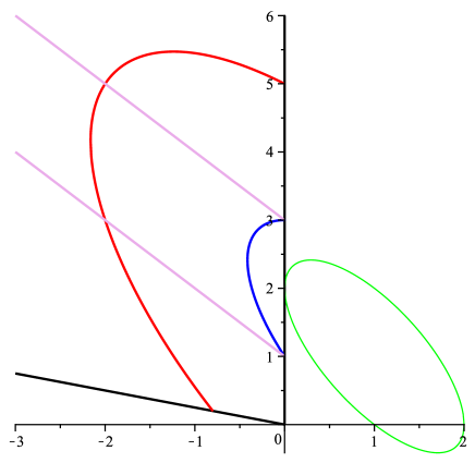
Figure 13. Domain lines in the $(q,\eta_{1})$ plane, for the $\eta_{2}=-q$ case. The two purple straight lines have for equations, $\eta_{1}=1-q$ and $\eta_{1}=3-q$. The green, blue and red ellipses have for respective equations $\hat{X}^{2}+Y^{2}=1,2,10$, with $\hat{X}=q-1,Y=\eta_{1}+q-2$, with a common center located at $(q,\eta_{1})=(1,1)$.

The results are summarized in Fig. 13. The blue and red ellipses in Fig. 13 above respectively correspond to the first $n=1$ and $n=2$ cases. Because of (4.65), these ellipses are images by the $(q\to q-2,\eta_{1}\to\eta_{1}+2)$ translation of the corresponding same color ellipses of Fig. 12 in Section 4.1, with a common center now located at $(q,\eta_{1})=(1,1)$. Note also that if the generalized spectrum is given in the whole region $D_{-q}$ by $\alpha_{0}^{+}$ in Eq. (4.62), then on the SLE_κ-line where $\kappa=2\eta_{1}=\eta_{2}/2=-q/2$ it coincides with the spectrum $\beta_{1}(2,q;\kappa=-q/2)=5-3q/2$, and there is no phase transition along that line, in contrast to the $(\eta_{2}=4-q)$-case. The phase transition now takes place on the $q=0=\eta_{2}$ line, at its $\eta_{1}=2$ contact point with the green ellipse, since the predicted spectrum $\alpha_{0}^{+}$ is there equal to $5-\eta_{1}$ for $0\leq\eta_{1}\leq 2$ and to $3$ for $\eta_{1}\geq 2$. This agrees with results (4.13), $\beta(2,0)=4$ for $\eta_{1}=1$, and (4.11), $\beta(2,0)=3$ for $\eta_{1}=3$.

Remark 4.3.

Alternative condition.

For completeness, let us also mention that the alternative condition in (4.72), $2n-(2\alpha+q-8)=0$ with $\alpha=\alpha_{0}^{\pm}$, yields $2n+q+\eta_{1}=\pm\sqrt{\hat{Z}}$, leading to $\eta_{1}+q-1=\frac{q(q-2)}{4(n+1)}-n$ and to the selection of the $(+)$-branch. From (4.71), one further needs to check that $(\eta_{1}+q+1)A_{1}^{n}=(\eta_{1}+q-1)A_{2}^{n}$ upon starting the recursion (4.67) from the null-eigenvector (4.66). Using again Mathematica® shows this equality not to hold, thus leading to no further solution.

4.2.4. General solution to the Fuchsian system

From the perspective of Fuchsian systems [IY08, LY19], the initial equations (4.53) for the vector function, $\vartheta(\xi):=(\theta_{0}(\xi),\theta_{1}(\xi),\theta_{2}(\xi))^{t}$ can be written under the matrix form,

$$\vartheta^{\prime}(\xi)=\frac{\mathbb{A}}{\xi}\vartheta(\xi)+\frac{\mathbb{B}}{1-\xi}\vartheta(\xi),$$

where matrices $\mathbb{A}$ and $\mathbb{B}$ do not depend on $\xi$. They are simply given here by

$$\mathbb{A}=\frac{1}{2}\begin{pmatrix}0&0&0\\ \eta_{1}+q-3&-(\eta_{1}+1)&0\\ 0&-4&q-2\end{pmatrix},$$ (4.77)

$$\mathbb{B}=\frac{1}{2}\begin{pmatrix}2(3-q)&2(q-2)&0\\ \eta_{1}+q-3&-2(\eta_{1}+q-3)&\eta_{1}+q-1\\ 0&-4&6\end{pmatrix}.$$ (4.78)

The discriminant of $\mathbb{B}$ is

$$\det(\mathbb{B}-\alpha\mathds{1}) =(1-\alpha)\left[\frac{1}{2}(\eta_{1}+q-3)(2\alpha+q-6)+(\alpha-2)(\alpha+q-3)\right]$$

$$=\frac{1}{2}(1-\alpha)E_{0}(\alpha)=\frac{1}{4}\det D_{0}(\alpha),$$

so that $\mathbb{B}$ has for eigenvalues the zeroes of $\det D_{0}$, $\alpha_{0}^{\pm}$ (4.62) and $1$.

For $\xi\to 1^{-}$, the vector functions $\vartheta(\xi)=(\theta_{0}(\xi),\theta_{1}(\xi),\theta_{2}(\xi))^{t}$, have for asymptotic behavior,

$$\vartheta(\xi)=(1-\xi)^{-\alpha_{0}^{+}}{\bf f}^{+}(\xi)+(1-\xi)^{-\alpha_{0}^{-}}{\bf f}^{-}(\xi)+(1-\xi)^{-1}{\bf f}^{1}(\xi),$$ (4.79)

where ${\bf f}^{\pm},{\bf f}^{1}$ are vector functions with Taylor series expansions in $\xi$. In the generic non-resonant case, where the eigenvalues do not differ by integer numbers, these functions converge at $\xi=1$ towards the eigenvectors of $\mathbb{B}$ corresponding to their respective eigenvalue powers $\alpha_{0}^{\pm},1$. In the resonant case, they can be polynomials in $\xi$, or can involve polynomials in $-\log(1-\xi)$, which then dominate the limit when $\xi\to 1^{-}$.

In the resonant case of the ${\mathcal{E}}_{n}$ ellipses of Section 4.2.3, we have $\alpha_{0}^{-}=\alpha_{0}^{+}-(2n-1)$ with $n\geq 1$. These vector functions are then simple polynomials, with

$${\bf f}^{+}(\xi)=(f_{0}(\xi),f_{1}(\xi),f_{2}(\xi))^{t},$$

and ${\bf f}^{-}(\xi)={\bf f}^{1}(\xi)={\bf 0}$. At $\xi=1$, ${\bf f}^{+}(\xi)$ becomes the eigenvector ${\bf f}^{+}(\xi=1)={\bf A}_{0}(\alpha_{0}^{+})$, as given in (4.66).

Let us conclude with the following Theorem.

Theorem 4.2.

The generalized integral means spectrum $\beta(2,q)$ of a whole-plane Lévy-Loewner process with Lévy symbols $\eta_{1}$ and $\eta_{2}=-q$ is given in the whole $D_{-q}$ domain (4.52) by $\alpha_{0}^{+}$ in Eq. (4.62).

Proof.

Because of (4.79), the generalized integral means spectrum must be equal to one of the three eigenvalues $\alpha_{0}^{+},\alpha_{0}^{-},1$. Eigenvalues $\alpha_{0}^{+}$ and $\alpha_{0}^{-}$ are equal only when $\hat{Z}=0$, i.e., on the green ellipse which lies outside $D_{-q}$, except for the point $P_{0}=(q=0,\eta_{1}=2)$. Therefore in $D^{*}_{-q}:=D_{-q}\setminus P_{0}$, we have $\alpha_{0}^{+}>\alpha_{0}^{-}$. One can also check that on $D_{-q}$, $\alpha_{0}^{+}>1$, whereas the equality $\alpha_{0}^{-}=1$ is realized in $D_{-q}$ on the branch of hyperbola of equation $(\eta_{1}+q-8)(q-4)=4$ with $q\leq 0$. We know that $\beta(2,q)=3-q=\alpha_{0}^{+}$ on the half-line $\eta_{1}=3-q,q\leq 0$, as well as $\beta(2,q)=4-q=\alpha_{0}^{+}$ on the half-line $\eta_{1}=1-q,q\leq 0$. Because of the Hölder inequality, the generalized integral means spectrum is convex in $(p,q)$ [DHLZ18], hence continuous. By continuity, $\beta(2,q)=\alpha_{0}^{+}$ on these integrability lines cannot jump to $\alpha_{0}^{-}<\alpha_{0}^{+}$ or $1<\alpha_{0}^{+}$ in $D^{*}_{-q}$, hence $\beta(2,q)=\alpha_{0}^{+}$ in the whole domain. At the singular point $P_{0}$ , the spectrum is still $\alpha_{0}^{+}$, with a change of its analytic form. ∎

Acknowledgements: This material is based upon work supported by the National Science Foundation under Grant No. DMS-1928930 while Bertrand Duplantier participated in the program “Analysis and Geometry of Random Spaces”, hosted by the Mathematical Sciences Research Institute in Berkeley, California, during the Spring 2022 semester. The work by Yong Han is supported by the National Natural Science Foundation of China under Grant No. 12131016. B.D. also wishes to warmly thank Emmanuel Guitter for his help with Mathematica® and the figures, and Thomas C. Halsey for a critical reading of the manuscript.

References

- [ABV16] Tom Alberts, Ilia Binder, and Fredrik Viklund. A dimension spectrum for SLE boundary collisions. Commun. Math. Phys., 343:273–298, 2016.
- [App09] David Applebaum. Lévy Processes and Stochastic Calculus. Cambridge Studies in Advanced Mathematics. Cambridge University Press, 2nd edition, 2009.
- [ASZ08] D. A. Adams, L. M. Sander, and R. M. Ziff. Harmonic Measure for Percolation and Ising Clusters Including Rare Events. Phys. Rev. Lett., 101:144102, 2008.
- [BD23] I. Binder and B. Duplantier. Multifractal properties of harmonic measure and rotation for Schramm-Loewner Evolution, 2023. In preparation.
- [BDZ17] Dmitry Beliaev, Bertrand Duplantier, and Michel Zinsmeister. Integral means spectrum of whole-plane SLE. Commun. Math. Phys., 353(1):119–133, 2017.
- [Bel19] Dmitry Beliaev. Conformal Maps and Geometry. World Scientific Publishing Europe Ltd, London, UK, 2019.
- [BGIR08] A Belikov, I A Gruzberg, and I. I Rushkin. Statistics of harmonic measure and winding of critical curves from conformal field theory. J. Phys. A: Math. Theor., 41(28):285006, 2008.
- [Bin97] Ilia Binder. Rotational Spectrum of Planar Domains. PhD thesis, California Institute of Technology, 1997.
- [BRGW05] E. Bettelheim, I. Rushkin, I. A. Gruzberg, and P. Wiegmann. Harmonic Measure of Critical Curves. Phys. Rev. Lett., 95:170602, 2005.
- [BS09] Dmitry Beliaev and Stanislas Smirnov. Harmonic measure and SLE. Commun. Math. Phys., 290(2):577–595, 2009.
- [CR08] Zhen-Qing Chen and Steffen Rohde. Schramm-Loewner equations driven by symmetric stable processes. Commun. Math. Phys., 285:799–824, 2008.
- [Dav88] F. David. Conformal Field Theories Coupled to -D Gravity in the Conformal Gauge. Mod. Phys. Lett. A, 3(17):1651–1656, 1988.
- [DB02] B. Duplantier and I. A. Binder. Harmonic Measure and Winding of Conformally Invariant Curves. Phys. Rev. Lett., 89:264101, 2002.
- [DB08] B. Duplantier and I. A. Binder. Harmonic measure and winding of random conformal paths: A Coulomb gas perspective. Nucl. Phys. B [FS], 802:494–513, 2008.
- [DHLZ18] Bertrand Duplantier, Xuan Hieu Ho, Thanh Binh Le, and Michel Zinsmeister. Logarithmic coefficients and generalized multifractality of whole-plane SLE. Commun. Math. Phys., 359(3):823–868, 2018.
- [DK89] J. Distler and H. Kawai. Conformal Field Theory and D Quantum Gravity. Nucl. Phys. B, 321:509–527, 1989.
- [DMS21] Bertrand Duplantier, Jason Miller, and Scott Sheffield. Liouville Quantum Gravity as a Mating of Trees. Astérisque., 427:1–258, 2021.
- [DNNZ15] Bertrand Duplantier, Chi Nguyen, Nga Nguyen, and Michel Zinsmeister. The coefficient problem and multifractality of whole-plane SLE & LLE. Ann. Henri Poincaré, 16(6):1311–1395, 2015.
- [DRSV14] Bertrand Duplantier, Rémi Rhodes, Scott Sheffield, and Vincent Vargas. Renormalization of Critical Gaussian Multiplicative Chaos and KPZ Relation. Commun. Math. Phys., 330(1):283 – 330, 2014.
- [DS09] B. Duplantier and S. Sheffield. Duality and KPZ in Liouville Quantum Gravity. Phys. Rev. Lett., 102:150603, 2009.
- [DS11a] B. Duplantier and S. Sheffield. Liouville Quantum Gravity and KPZ. Invent. Math., 185:333–393, 2011.
- [DS11b] B. Duplantier and S. Sheffield. Schramm-Loewner Evolution and Liouville Quantum Gravity. Phys. Rev. Lett., 107:131305, 2011.
- [Dub09] Julien Dubédat. Duality of Schramm-Loewner evolutions. Ann. Sci. Éc. Norm. Supér. (4), 42(5):697–724, 2009.
- [Dup99a] B. Duplantier. Harmonic Measure Exponents for Two-Dimensional Percolation. Phys. Rev. Lett., 82:3940–3943, 1999.
- [Dup99b] B. Duplantier. Two-Dimensional Copolymers and Exact Conformal Multifractality. Phys. Rev. Lett., 82:880–883, 1999.
- [Dup00] Bertrand Duplantier. Conformally invariant fractals and potential theory. Phys. Rev. Lett., 84(7):1363–1367, 2000.
- [Dup03] Bertrand Duplantier. Higher conformal multifractality. J. Statist. Phys., 110(3-6):691–738, 2003.
- [Dup04] B. Duplantier. Conformal fractal geometry & boundary quantum gravity. In M. L. Lapidus and M. van Frankenhuysen, editors, Fractal geometry and applications: a jubilee of Benoît Mandelbrot, Part 2, volume 72 of Proc. Sympos. Pure Math., pages 365–482. Amer. Math. Soc., Providence, RI, 2004.
- [Dup06] B. Duplantier. Conformal Random Geometry. In A. Bovier, F. Dunlop, F. den Hollander, A. van Enter, and J. Dalibard, editors, Mathematical Statistical Physics (Les Houches Summer School, Session LXXXIII, 2005), pages 101–217. Elsevier B.V., Amsterdam, 2006.
- [FP85] U. Frisch and G. Parisi. Turbulence and predictability in geophysical fluid dynamics and climate dynamics. In M. Ghil, R. R. Benzi, and G. Parisi, editors, Proceedings of the International School of Physics Enrico Fermi, course LXXXVIII, pages 84–87. North Holland, New York, 1985.
- [GM08] John B. Garnett and Donald E. Marshall. Harmonic measure, volume 2 of New Mathematical Monographs. Cambridge University Press, Cambridge, 2008. Reprint of the 2005 original.
- [GMS18] Ewain Gwynne, Jason Miller, and Xin Sun. Almost sure multifractal spectrum of Schramm-Loewner evolution. Duke Math. J., 167(6):1099–1237, 2018.
- [Has02] M. B. Hastings. Exact Multifractal Spectra for Arbitrary Laplacian Random Walks. Phys. Rev. Lett., 88:055506, 2002.
- [HJK+86a] T. C. Halsey, M. H. Jensen, L. P. Kadanoff, I. Procaccia, and B. I. Shraiman. Fractal measures and their singularities - The characterization of strange sets. Phys. Rev. A, 33:1141–1151, 1986.
- [HJK+86b] T. C. Halsey, M. H. Jensen, L. P. Kadanoff, I. Procaccia, and B. I. Shraiman. Fractal measures and their singularities: The characterization of strange sets; Erratum: [Phys. Rev. A 33, 1141 (1986)]. Phys. Rev. A, 34:1601–1601, 1986.
- [Ho16] Xuan Hieu Ho. On multifractality, Schwarzian derivative and asymptotic variance of whole-plane SLE. PhD Thesis, Université d’Orléans, December 2016.
- [Ho22] Xuan Hieu Ho. Generalized integral means spectrum of SLE. arXiv:2203.10782v1, 2022.
- [HP83] H. G. E. Hentschel and I. Procaccia. The infinite number of dimensions of probabilistic fractals and strange attractors. Physica D, 8:435–444, 1983.
- [IY08] Yulij Ilyashenko and Sergei Yakovenko. Lectures on analytic differential equations, volume 86 of Graduate Studies in Mathematics. American Mathematical Society, Providence, RI, 2008.
- [JVL12] F. Johansson Viklund and G.F. Lawler. Almost sure multifractal spectrum for the tip of an SLE curve. Acta Math., 209(2):265–322, 2012.
- [KNK04] Wouter Kager, Bernard Nienhuis, and Leo P. Kadanoff. Exact solutions for Loewner evolutions. J. Stat. Phys., 115(3-4):805–822, 2004.
- [KPZ88] V. G. Knizhnik, A. M. Polyakov, and A. B. Zamolodchikov. Fractal Structure of D-quantum gravity. Mod. Phys. Lett. A, 3:819–826, 1988.
- [Law05] Gregory F. Lawler. Conformally invariant processes in the plane, volume 114 of Mathematical Surveys and Monographs. American Mathematical Society, Providence, RI, 2005.
- [Lin05] Joan Lind. A sharp condition for the Loewner equation to generate slits. Ann. Acad. Sci. Fenn., 30:143–158, 2005.
- [LMR10] Joan Lind, Donald E. Marshall, and Steffen Rohde. Collisions and spirals of Loewner traces. Duke Math. J., 154(3):527–573, 09 2010.
- [Lou12] Igor Loutsenko. :correlation functions in the coefficient problem. J. Phys. A: Math. Theor., 45(27):275001, 10, 2012.
- [LW99] G. F. Lawler and W. Werner. Intersection exponents for planar Brownian motion. Ann. Probab., 27(4):1601–1642, 1999.
- [LY13] Igor Loutsenko and Oksana Yermolayeva. Average harmonic spectrum of the whole-plane SLE. J. Stat. Mech. Theory Exp., page P04007, 2013.
- [LY14] Igor Loutsenko and Oksana Yermolayeva. New exact results in spectra of stochastic Loewner evolution. J. Phys. A: Math. Theor., 47(16):165202, 15, 2014.
- [LY19] Igor Loutsenko and Oksana Yermolayeva. Stochastic Loewner evolutions, Fuchsian systems and orthogonal polynomials. J. Phys. A: Math. Theor., 52(43):435202, 2019.
- [Mak98] N. G. Makarov. Fine structure of harmonic measure. Rossiĭskaya Akademiya Nauk. Algebra i Analiz, 10:1–62, 1998. English translation in St. Petersburg Math. J. 10: 217-268 (1999).
- [Man74] B. B. Mandelbrot. Intermittent turbulence in self-similar cascades: Divergence of high moments and dimension of the carrier. J. Fluid. Mech., 62:331–358, 1974.
- [MR05] Donald E. Marshall and Steffen Rohde. The Loewner differential equation and slit mappings. J. Am. Math. Soc., 18(4):763–778, 2005.
- [Pai00] Paul Painlevé. Analyse des travaux scientifiques. Gauthier-Villars, Paris, 1900. Reprinted in Librairie Scientifique et Technique, Albert Blanchard, Paris, 1967, pp. 1-2; reproduced in Oeuvres de Paul Painlevé, Éditions du CNRS, Paris, 1972-1975, vol. 1, pp. 72-73.
- [RBGW07] I. Rushkin, E. Bettelheim, I. A. Gruzberg, and P. Wiegmann. Critical curves in conformally invariant statistical systems. J. Phys. A: Math. Gen., 40:2165–2195, 2007.
- [RS05] Steffen Rohde and Oded Schramm. Basic properties of SLE. Ann. of Math. (2), 161(2):883–924, 2005.
- [RV11] R. Rhodes and V. Vargas. KPZ formula for log-infinitely divisible multifractal random measures. ESAIM: Probability and Statistics, 15:358–371, 2011.
- [Sch00] Oded Schramm. Scaling limits of loop-erased random walks and uniform spanning trees. Israel J. Math., 118:221–288, 2000.
- [Sch20] L. Schoug. A multifractal boundary spectrum for SLE curve. Probab. Theory Relation. Fields, 178:173–233, 2020.
- [She16] Scott Sheffield. Conformal weldings of random surfaces: SLE and the quantum gravity zipper. Ann. Probab., 44(5):3474 – 3545, 2016.
- [Zha08] Dapeng Zhan. Duality of chordal SLE. Invent. Math., 174(2):309–353, 2008.