Replacing Labeled Real-image Datasets with Auto-generated Contours

Abstract

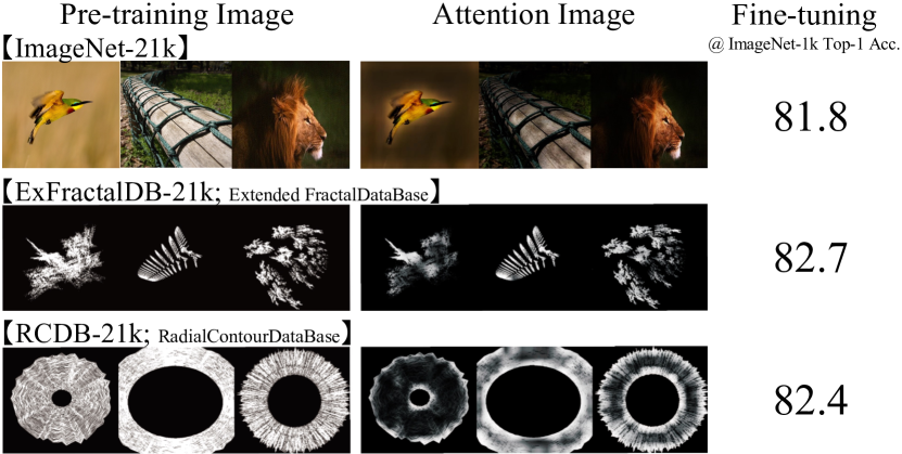
In the present work, we show that the performance of formula-driven supervised learning (FDSL) can match or even exceed that of ImageNet-21k without the use of real images, human-, and self-supervision during the pre-training of Vision Transformers (ViTs). For example, ViT-Base pre-trained on ImageNet-21k shows 81.8% top-1 accuracy when fine-tuned on ImageNet-1k and FDSL shows 82.7% top-1 accuracy when pre-trained under the same conditions (number of images, hyperparameters, and number of epochs). Images generated by formulas avoid the privacy/copyright issues, labeling cost and errors, and biases that real images suffer from, and thus have tremendous potential for pre-training general models.

To understand the performance of the synthetic images, we tested two hypotheses, namely (i) object contours are what matter in FDSL datasets and (ii) increased number of parameters to create labels affects performance improvement in FDSL pre-training. To test the former hypothesis, we constructed a dataset that consisted of simple object contour combinations. We found that this dataset can match the performance of fractals. For the latter hypothesis, we found that increasing the difficulty of the pre-training task generally leads to better fine-tuning accuracy.

Abstract

In the present work, we show that the performance of formula-driven supervised learning (FDSL) can match or even exceed that of ImageNet-21k without the use of real images, human-, and self-supervision during the pre-training of Vision Transformers (ViTs). For example, ViT-Base pre-trained on ImageNet-21k shows 81.8% top-1 accuracy when fine-tuned on ImageNet-1k and FDSL shows 82.7% top-1 accuracy when pre-trained under the same conditions (number of images, hyperparameters, and number of epochs). Images generated by formulas avoid the privacy/copyright issues, labeling cost and errors, and biases that real images suffer from, and thus have tremendous potential for pre-training general models.

To understand the performance of the synthetic images, we tested two hypotheses, namely (i) object contours are what matter in FDSL datasets and (ii) increased number of parameters to create labels affects performance improvement in FDSL pre-training. To test the former hypothesis, we constructed a dataset that consisted of simple object contour combinations. We found that this dataset can match the performance of fractals. For the latter hypothesis, we found that increasing the difficulty of the pre-training task generally leads to better fine-tuning accuracy.

1 Introduction

Image recognition has greatly benefited from labeled real-image datasets. Conventional image datasets comprise real images of various objects on a general background annotated by humans. A visual representation can be acquired by learning from real images with such annotations. Supervised learning (SL) is the most trusted approach for this task. However, in recent years self-supervised learning (SSL) has gained ground [16, 8, 6, 7, 9].

SSL methods have recently been used to pre-train Vision Transformers (ViTs) [13]; however, datasets with hundreds of millions of images are required [11, 32]. The learning methods DINO [5] and MoCoV3 [10] show that it is possible to train on relatively small datasets such as ImageNet-1k (ILSVRC) [31]. SSL methods remove the time-consuming labeling of a dataset, but do not address privacy, copyright, and societal biases when real images are used [37, 2].

Figure 1: We have found that vision transformers (ViT) can be successfully pre-trained without real images, human- and self-supervision, and can exceed the accuracy of ImageNet-21k pre-training when fine-tuned on ImageNet-1k. We constructed a new dataset Radial Contour DataBase (RCDB) based on the assumption that contours are what matter for the pre-training of ViT. RCDB also exceeded the performance of ImageNet-21k pre-training, while consisting only of contours.

Formula-driven supervised learning (FDSL) trains on synthetic images generated by mathematical formulas and thus avoids such issues [21, 27, 19, 20, 3, 1]. The images can be categorized and labeled automatically based on the parameters of the equations used to generate them. Because the images are generated by mathematical formulas, they avoid the ethical problems associated with labeled real-image datasets. If FDSL can be used to pre-train models to the same accuracy as that achieved with real images, it could replace SL/SSL to avoid ethical issues.

To improve FDSL methods, Kataoka et al. [21] used fractal geometry based on the assumption that fractals are a natural phenomenon. They found that the actual performance depends on the number of hyperparameters in order to create FDSL datasets. In the present work, we investigate the most influential factors for generating synthetic images from formulas and the possibility of using alternatives to fractals. We establish some basic guidelines that lead to better FDSL methods to avoid the iterative process of rendering and pre-training.

In this paper, we enhance the performance of FDSL in the context of pre-training ViTs [13]. We first test the following two hypotheses. Hypothesis 1: object contours are what matter in FDSL datasets. Hypothesis 2: increased number of parameters affects performance improvement in FDSL pre-training. Preliminary study that led to these hypotheses are shown in Section 3.1. Through the validation of these hypotheses, we generate an improved synthetic dataset that allowed us to pre-train ViTs with a higher accuracy than that of real-image datasets.

Impact of the paper. We show that the performance of pre-training ViTs with FDSL can match or even exceed that of pre-training ViT with ImageNet-21k. When fine-tuned on ImageNet-1k, ViT-Base pre-trained on ImageNet-21k has a top-1 accuracy of 81.8% and that pre-trained on Extended Fractal DataBase (ExFractalDB) and Radial Contour DataBase (RCDB) (which has the same number of classes and instances per class) has an accuracy of 82.7 and 82.4%, respectively (Figure 1, Table 8).

Effect of Hypothesis 1. To understand the performance of fractal images, we explore alternative formulas for generating images. In our preliminary study (see Section 3.1), we found that the object contours in the fractal images play an important role. Therefore, we created a dataset that is specifically tailored to drawing object contours (called RCDB). The performance of this dataset matches that of FractalDB (Table 3).

Effect of Hypothesis 2. We find that higher complexity of the mathematically generated images improves the accuracy of FDSL (Table 5). The complexity of the images can be increased by adjusting the parameters of the formula-driven image generation. For example, RCDB becomes more complex when the number of vertices is increased; its complexity can also be changed by adjusting the contour smoothness, number of polygons, and radius (Table 2). The complexity of FractalDB can be increased by applying an iterative function system (IFS) in three-dimensional (3D) space instead of two-dimensional (2D) space.

2 Related work

Supervised training is the most reliable training mode in terms of accuracy. It is thus used as a baseline to measure the effectiveness of other training modes. Representative datasets such as ImageNet [11, 31] and Places [40] are collected, labeled, and cross-checked using cloud sourcing.

Huge models based on ViTs have recently achieved high accuracy when trained on enormous datasets. It can take hundreds of millions of man hours to collect the kind of datasets required to pre-train ViT architectures. Moreover, the resulting datasets, such as JFT-300M/3B [38] and Instagram-3.5B (IG-3.5B) [26], are not currently publicly available, which severely limits the accessibility and reproducibility of ViT research.

SSL removes the annotation cost by automatically generating labels according to rules that can be learned  [12, 39, 29, 30, 15]. The performance of contrastive SSL methods [16, 8, 6, 7] is close to that of SL. For example, SimSiam [9] can learn without negative samples and with smaller batch sizes. DINO [5] and MoCoV3 [10] have demonstrated SSL on ViTs.

Labeling cost is not the only problem with large image datasets. Popular datasets have privacy and fairness issues, such as the ethical problems [37, 4] in ImageNet (human-related labels) [11] and 80M Tiny Images [33], which have led to the suspension of their publication. SSL can eliminate labeling cost but it does not address ethical issues. Even PASS [2], a database of images licensed under a Creative Commons (CC-BY) license that excludes images of people, might have some harmful content.

FDSL has the potential to entirely remove such ethical issues because it can generate and label the dataset using only equations and their parameters. There has been considerable interest in FDSL [21, 19, 20, 3, 1]. However, the performance of existing FDSL fails to match that of SL and thus FDSL methods are not yet practical alternatives.

Nakashima et al. used FractalDB for pre-training ViTs and matched the accuracy of SSL (SimCLRV2) [27]. However, they studied only one dataset (FractalDB) and did not analyze the performance of FDSL or its failure modes. In the present work, we perform a wider search of possible FDSL methods, and analyze the characteristics that correlate with good pre-training performance. We also show the range of parameters and configurations for which FDSL completely fails, providing insight into what constitutes a favorable synthetic image dataset for pre-training ViTs.

3 Method

We first show the results of our preliminary study from which we deduced the hypotheses that (i) object contours are what matter in image representation and (ii) increased number of parameters affects performance improvement in FDSL pre-training. Then, we propose a set of mathematically generated datasets that have varying degrees of complexity in these two aspects to verify our hypotheses.

To verify the hypothesis regarding the importance of object contours in images, we create the dataset RCDB. To verify the second hypothesis, we increase the number of parameters in the equations used to generate the images in ExFractalDB and RCDB and increase the size of the dataset.

3.1 Preliminary study

As a baseline, we first report the results for FractalDB-1k [21], which has 1,000 classes and 1,000 instances per class. We select ViT-tiny with $16\times 16$ [pixels] patches as the baseline model. The hyperparameters and data augmentation are selected according to previous work [34].

Hypothesis 1: object contours are what matter in FDSL datasets. The attention map for the training of ViTs with FractalDB-1k is shown in Figure 2, where attention is focused on the outer contours of the fractals. The same behavior was observed across other images in the dataset. We previously believed that the ability of fractals to generate recurring patterns found in nature is what allows them to be used as alternatives to real images. However, these preliminary experiments suggest that the same effectiveness can be achieved by generating object contours with a sufficiently high complexity.

Figure 2: Fractal images and attention maps on object contours.

Table 1: Relationship between FractalDB-1k and labeling. FDSL (Fractal) corresponds to the the original FractalDB, and FDSL (Fractal, restricted) varies only three parameters $(a_{i},c_{i},e_{i})$ and the other three $(b_{i},d_{i},f_{i})$ are fixed. Best values are in bold.

Type	C10	C100	Cars	Flowers
SSL (MoCov2)	92.6	73.7	33.6	93.9
SSL (SimCLRv2)	94.8	78.9	61.7	99.6
FDSL (Fractal, restricted)	96.8	82.0	86.8	98.2
FDSL (Fractal)	97.0	82.4	87.9	98.3

Hypothesis 2: Increased number of parameters in FDSL pre-training. For both FDSL and SSL, manual labeling is unnecessary. FDSL automatically labels the dataset during its creation, which is fundamentally different from SSL. To investigate the role of labels in FDSL, we compare the pre-training of fractal images with FDSL and SSL, respectively (Table 1). For SSL, we select MoCoV2 and SimCLRV2. We compare two types of FractalDB, the original method with 6 parameters, FDSL (Fractal), and another that varies only three parameters while the other three are fixed, FDSL (Fractal, restricted; See supplementary material for further details). The three parameters $(a_{i},c_{i},e_{i})$ that we changed, were set to match the FractalDB paper [21].

Our results show that FDSL yields higher accuracy than SSL when using FractalDB. This result indicates that it is better to use labels from a mathematical formula that generates an image pattern with FDSL, than to assign an external label with SSL. We also find that FractalDB created with a larger number of parameters leads to higher accuracy. We therefore hypothesize that the accuracy of FDSL can be improved by increasing the parameters in equations to create FDSL labels.

3.2 Formula-driven supervised learning

Figure 3: Procedure for generating radial contours $\mathcal{R}$. Example with $n=3$ vertices and $N=5$ polygons is shown.

FDSL automatically generates image patterns and their corresponding labels based on formulas. Unlike the pre-training in SL/SSL, FDSL does not require real images.

Definition of FDSL. Let $\phi_{\theta}$ be a network to be pre-trained with parameter set $\theta$. FDSL solves the following problem:

$$\hat{\theta}=\mathop{\rm argmin}_{\theta}\limits\mathbb{E}_{({\bm{x}},y)}[\mathcal{L}(\phi_{\theta}({\bm{x}}),y)]$$ (1)

where ${\bm{x}}$ is the synthetic image, $y$ is the corresponding label, and $\mathcal{L}$ is a loss function. The synthetic images are generated by ${\bm{x}}=F_{y}(s)$, where $y\in\{1,2,\cdots,C\}$ is a discrete label and $F_{y}$ is the $y$-th mathematical formula used to generate intra-class images. Note that to create intra-class variation, $F_{y}$ involves randomness, so a random seed $s$ is input. This leads to a two-step sampling of $({\bm{x}},y)$ in Eq. (1), where $y$ is first uniformly sampled and then image pattern ${\bm{x}}$ is generated with $F_{y}(s)$ using the uniformly sampled seed $s$.

3.2.1 Radial Contour Database (RCDB)

Definition of RCDB. The proposed radial contour $\mathcal{R}\subset\mathbb{R}^{2}$ is an object made by superimposing polygons. It is defined by a union set of polygons as follows:

$$\mathcal{R}=\bigcup_{p=1}^{N}R_{p}$$ (2)

where $R_{p}$ is the $p$-th polygon and $N$ is the number of polygons. Each polygon $R_{p}$ consists of $n$ edges as follows:

$$R_{p}=\bigcup_{j=1}^{n}e({\bm{v}}^{(p)}_{j-1},{\bm{v}}^{(p)}_{j})$$ (3)

where ${\bm{v}}^{(p)}_{j}\in\mathbb{R}^{2}$ is the $j$-th vertex. Note that we define vertices for $j=0,1,\cdots,n$ but ${\bm{v}}^{(p)}_{0}={\bm{v}}^{(p)}_{n}$ is redundant. $e(\cdot,\cdot)$ is the edge between two vertices given by

$$e({\bm{p}},{\bm{q}})=\{t{\bm{p}}+(1-t){\bm{q}}+{\bm{c}}\in\mathbb{R}^{2}:0\leq t\leq 1\}$$ (4)

where ${\bm{c}}$ is the center of the polygon.

Our algorithm makes polygons from the center to the border as follows. The first polygon $R_{1}$ is made by resizing an $n$-regular polygon, i.e., the vertices are given by

$${\bm{v}}^{(1)}_{j}=r\begin{pmatrix}o_{x}\cos\left(2\pi j/n\right)\\ o_{y}\sin\left(2\pi j/n\right)\\ \end{pmatrix}$$ (5)

for $j=0,1,2,\cdots n$ with radius $r$ and a resizing factor ${\bm{o}}=(o_{x},o_{y})$. This step is illustrated in Figure 3(a).

In the second step, vertices are copied and moved toward the border. Specifically, given the vertices for $R_{p-1}$, new vertices for $R_{p}$ are defined as

$${\bm{v}}^{(p)}_{j}={\bm{v}}^{(p-1)}_{j}+\begin{pmatrix}(l_{w}+\lambda_{x}\epsilon_{j,p-1})\cos\left(2\pi j/n\right)\\ (l_{w}+\lambda_{y}\epsilon_{j,p-1})\sin\left(2\pi j/n\right)\\ \end{pmatrix}$$ (6)

where $l_{w}$ is the line width, ${\bm{\epsilon}}_{j}=(\epsilon_{j,1},\epsilon_{j,2},\cdots,\epsilon_{j,N})$ is a one-dimensional Perlin noise sequence, and ${\bm{\lambda}}=(\lambda_{x},\lambda_{y})$ is a noise scaling factor. This step is repeated for $p=2,3,\cdots N$. Examples of $R_{2}$ and $\mathcal{R}$ are shown in Figures 3(b) and (c), respectively. Finally, the radial contour is rendered with a line width of $l_{w}$ in white over a black background. The image size is $512\times 512$.

Table 2: Parameter set ($\eta$) for RCDB categories.

Parameter set ($\eta$)
# of polygons ($N$)	{1, 2, 3, … , 200}
# of vertices ($n$)	{3, 4, 5, … , 502}
Radius ($r$)	[0.0, 100.0]
Line width ($l_{w}$)	[0.0, 0.1]
Resizing factor (${\bm{o}}$)	[1.0, 4.0]
Perlin noise (${\bm{\lambda}}$)	[0.0, 4.0]

RCDB-1k. Let $\eta=(N,n,r,l_{w},{\bm{o}},{\bm{\lambda}})$ be a hyperparameter set for generating radial contours. The proposed database consists of $C=$ 1k radial contour classes, each with a parameter set $\eta_{y}\ (y\in\{1,2,\cdots,C\})$. With the above generation procedure denoted as $G_{\text{RC}}$, the definition of $F_{y}$ in this database is given by $F_{y}(s)=G_{\text{RC}}(\eta_{y},s)$, where random seed $s$ is used to randomly choose the center ${\bm{c}}$ in Eq. (4) and generate one-dimensional Perlin noise sequences. The hyperparameters are uniformly distributed over the range shown in Table 2. For each class, 1k images are generated.

Scaling RCDB. To explore the possibility of large-scale RCDB pre-training, we prepare three more databases with the number of classes $C=$ 10k, 21k, and 50k. The number of images per class is set to 1k for all databases.

3.2.2 Extended FractalDB (ExFractalDB)

FractalDB. The original FractalDB proposed in [21] consists of 2D fractal images generated by an IFS. It has $C$ fractal classes, each of which has a hyperparameter set $\eta_{y}$ to generate fractals as $F_{y}(s)=G_{\text{IFS}}(\eta_{y},s)$, where $G_{\text{IFS}}$ is the rendering procedure based on IFS (see [21] for details) and $s$ is a random seed used to create intra-class variation. The hyperparameter $\eta_{y}=\{(w_{i},p_{i})\}_{i=1}^{N}$ consists of affine transformation functions $w_{i}:\mathbb{R}^{2}\to\mathbb{R}^{2}$ and a probability mass function $p_{i}$. FractalDB consists of $C=$1k classes, each with 1k randomly generated images.

ExFractalDB. MV-FractalDB [36] consists of 2D images that are projections of 3D fractals. The fractals are generated by 3D-IFS, which replaces the 2D affine transformation functions in $\eta_{y}$ with 3D ones, i.e., $w_{i}:\mathbb{R}^{3}\to\mathbb{R}^{3}$. The generated fractals are projected onto images via a virtual camera. ExFractalDB consists of $C=$1k classes. MV-FractalDB generates 12 images from fixed viewpoints, whereas ExFractalDB randomly selects and projects 2D images from 3D models.

Scaling ExFractalDB.. The potential of ViTs can only be realized through pre-training on huge datasets. However, previous work on FDSL pre-trained models on only relatively small datasets (on the order of 1M images). In the present work, we increase the size of the dataset to 10M, 20M, and 50M by simply increasing the number of classes, which is a trivial task for FDSL. This results in datasets with $C=$ 10k, 21k, and 50k, respectively. For each class, 25 3D fractal instances are generated. To increase the variation of the projected images, each instance is captured by a virtual camera from 40 positions, which are randomly and uniformly chosen from the surface of a unit sphere. As a result, $25$ [instances] $\times$ $40$ [viewpoints] $=1,000$ [images] are generated for each class.

See supplementary material for further details of FDSL datasets and pre-training.

4 Experiments

4.1 Verification of Hypotheses 1 and 2

In the verification, we choose the same datasets for fine-tuning as those in previous studies [34, 27], namely CIFAR-10/100 (C10/C100) [23], Stanford Cars (Cars) [22], and Flowers [28]. We use the same hyperparameters and data augmentation as those in [34]. FractalDB in these experiments has 1k classes, each with 1k instances. We update all layers during the pre-training and fine-tuning for all experiments. The following tables and their description correspond to Hypotheses 1 or 2.

Table 3: Comparison of FDSL methods. Hereafter, the best values are in bold.

Pre-training	C10	C100	Cars	Flowers
Scratch	78.3	57.7	11.6	77.1
Perlin Noise [21]	95.0	78.4	70.6	96.1
Dead Leaves [3]	95.9	79.6	72.8	96.9
Bezier Curves [21]	96.7	80.3	82.8	98.5
RCDB	96.8	81.6	84.2	98.7
FractalDB [27]	96.8	81.6	86.0	98.3

Table 4: Relationship between #vertices and accuracy in RCDB.

#Vertices	C10	C100	Cars	Flowers
3–102	95.5	79.4	78.4	96.4
103–202	94.2	76.3	55.8	95.9
203–302	71.3	46.9	4.9	49.8
303–402	59.4	33.9	2.5	26.8
403–502	40.1	13.6	0.8	5.3
3–502	96.4	80.7	83.0	98.5

Hypothesis 1: Comparison of FDSL methods (Table 3). We compare various types of mathematically generated dataset. Perlin noise and Bezier curves are from [21].

The results show that pre-training with RCDB and FractalDB give the highest fine-tuning accuracy, closely followed by BezierCurveDB. In RCDB, we only changed the number of vertices ($n$ in parameter set $\eta$). Regarding Hypothesis 1, we confirm that image representation using object contours tends to yield higher scores.

Hypothesis 1: Complexity of object contours in RCDB (Table 4). The complexity of the object contours in RCDB can be controlled by changing the number of vertices. We split the classes depending on the number of vertices.

Table 4 shows the results of RCDB for various ranges of categories. A comparison of the results obtained with 3–502 vertices (500 classes) and 3–102 vertices (100 classes) indicates that there exists an optimal degree of contour complexity. For ViTs, the best results are obtained with 103–202 vertices (100 classes); accuracy saturates at about 203–302 vertices (100 classes). Pre-training on RCDB with 203–302, 303–402, and 403–502 vertices led to lower scores than those for training from scratch (Table 9). This means that overly complicated object contours inhibit the acquisition of visual representation during the pre-training phase.

Hypothesis 2: Increased number of parameters in FDSL pre-training (Table 5). We increase the number of parameters to create FDSL labels. The results for Bezier Curves (BC; See supplementary material for further details), RCDB, and ExFractalDB are shown in Table 5.

Table 5: Effect of increased parameters in FDSL methods. BC stands for Bezier curves. Values in parentheses indicate the difference from the case with fewer parameters.

Pre-training	C10	C100	Cars	Flowers
BC	96.9 (0.2)	81.4 (1.1)	85.9 (3.1)	97.9 (-0.6)
RCDB	97.0 (0.2)	82.2 (0.6)	86.5 (2.4)	98.9 (0.2)
ExFractalDB	97.2 (0.4)	81.8 (0.2)	87.0 (1.0)	98.9 (0.6)

(a) $N$

(b) $r$

(c) $l_{w}$

(d) ${\bf o}$

(e) ${\bf\lambda}$

Figure 4: Parameter tuning on RCDB. Tuning was conducted with {C10, C100, Cars, Flowers}. The values in the graphs show the average rates on the four datasets.

Table 6: Comparisons of class definition type (from 2D IFS and 3D IFS) and instance augmentation (MV-FractalDB: fixed viewpoints and ExFractalDB: random viewpoints).

Pre-training	IFS	C10	C100	Cars	Flowers
FractalDB [21]	2D	96.8	81.6	86.0	98.3
MV-FractalDB [36]	3D	96.9	81.4	86.5	98.5
ExFractalDB	3D	97.2	81.8	87.0	98.9

(a) C10

(b) C100

(c) Cars

(d) Flowers

(e) RCDB w/ or w/o corruption

(f) (Left, center-left) Point rendering in FractalDB-1k with 10k and 50k points. We executed pre-training with {500, 1k, 10k, 50k, 100k, 200k} points in FractalDB-1k. (Center-right, right) The attention maps with the pre-trained models on FractalDB with 10k and 50k points, respectively.

(g) (Left) An example of RCDB with broken contours. We deliberately draw 1k lines with the same color as the background. (Center, right) Attention maps with the pre-trained models on RCDB with and without broken object contours, respectively.

Figure 5: Results, image examples, and attention maps in point-rendered FractalDB-1k (a, b, c, d, f) and RCDB with corruption (e, g). Although the fractal images with 50k (or higher) points and radial contours successfully trained the visual representations, the fractal images with 10k (or lower) points and radial contours with corruption failed.

(a) Examples of LineDB.

(b) Effect of #categories on accuracy.

Figure 6: Pre-training with line counting.

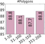
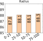
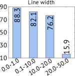
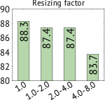
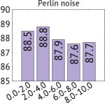
Hypothesis 2: Parameter search for RCDB (Figures 4(a)–4(e)). We explored the parameter set $\eta$ in order to combine these parameters in addition to the #vertices. Figures 4(a)–4(e) respectively show the effects of the number of polygons, radius, line width, resizing factor, and Perlin noise on accuracy. The parameters for RCDB in Table 2 are based on the results of this parameter search.

Hypothesis 2: Comparison of FractalDB [21], MV-FractalDB [36], and ExFractalDB (Table 6). ExFractalDB renders 3D fractals and projects them onto a 2D image. MV-FractalDB uses a fixed perspective when projecting 3D fractals onto 2D images; however, the present work uses a random perspective. MV-FractalDB labels the images according to the perspective in addition to the class of fractals; however, we do not consider the perspective labels.

As shown in the visualization (Figure 1), acquiring 2D images from a 3D model sharpens attention to multiple locations that seems to be useful for classification (unlike the attention to contours in Figure 2), and improves the accuracy itself.

4.2 Failure modes of FDSL

We have shown that pre-training with synthetic images that consist of only simple contours can match the accuracy of real images even at a fairly large scale. We now investigate when and how FDSL can fail.

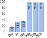
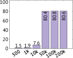
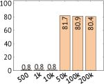
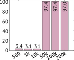
Minimum number of rendering points. We investigate the minimum number of points used in the rendering of fractals in FractalDB. Figure 5 shows the results and image examples in the point-rendered FractalDB. According to Figures 5(a)–5(d), the pre-trained models acquire a good representation when the number of fractal points is 50k or higher, at which point the fractal images start to form a contour (Figure 5(f)).

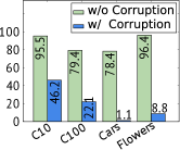
Adding corruption (broken object contours). We verify RCDB images with and without broken object contours, as shown in Figure 5(g). We deliberately draw 1k lines with the same color as the background. The lengths and positions of the lines are fully randomized. We adjust the thickness of the lines so that the object contours of RCDB are corrupted but the main frame does not disappear like in Figure 5(g). From the results in Figure 5(e), the rates change from {95.5, 79.4, 78.4, 96.4} with corruption to {46.2, 22.1, 1.1, 8.8} without corruption. These results support Hypothesis 1, namely that object contours are what matter in FDSL datasets.

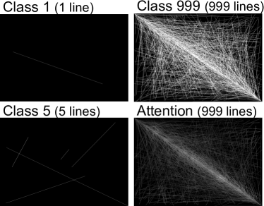
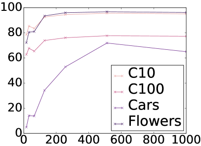
Minimum simplicity of images for pre-training ViTs. We create an extremely simple dataset with images that only contain randomly drawn lines (LineDB). The classes are assigned by counting the number of lines in each image. In this experiment, we assign LineDB-{16, 32, 64, 128, 256, 512, 1,000} categories in the pre-training phase (see Figure 6). LineDB is useful for pre-training. The model pre-trained with LineDB-512 had {95.6, 77.7, 71.9, 96.8} on {C10, C100, Cars, Flowers} (much higher than those for scratch training in Table 9). However, the pre-training effect slightly decreases for 1k categories. This is related to the optimal degree of contour complexity shown in Table 4. Moreover, for the dataset to have a positive pre-training effect, consistent labels need to be assigned to non-trivial images. The performance of LineDB-512 with random permutation was very low, with {13.5, 1.9, 0.8, 3.4} on {C10, C100, Cars, Flowers}.

Table 7: Comparison of ImageNet-1k fine-tuning. Accuracies obtained with ViT-Ti/B architectures are listed. 21k/50k indicates the number of classes in the pre-training phase. Best and second-best values for a given dataset are in underlined bold and bold, respectively. Pre-training Img Type ViT-Ti ViT-B Scratch – – 72.6 79.8 ImageNet-21k Real SL 74.1 81.8 FractalDB-21k Synth FDSL 73.0 81.8 FractalDB-50k Synth FDSL 73.4 82.1 ExFractalDB-21k Synth FDSL 73.6 82.7 ExFractalDB-50k Synth FDSL 73.7 82.5 RCDB-21k Synth FDSL 73.1 82.4 RCDB-50k Synth FDSL 73.4 82.6     Table 8: Comparison of object detection and instance segmentation. Several pre-trained models were validated on COCO dataset. Best values at each learning type are in bold. Pre-training COCO Det COCO Inst Seg AP50 / AP / AP75 AP50 / AP / AP75 Scratch 63.7 / 42.2 / 46.1 60.7 / 38.5 / 41.3 ImageNet-1k 69.2 / 48.2 / 53.0 66.6 / 43.1 / 46.5 ImageNet-21k 70.7 / 48.8 / 53.2 67.7 / 43.6 / 47.0 ExFractalDB-1k 69.1 / 48.0 / 52.8 66.3 / 42.8 / 45.9 ExFractalDB-21k 69.2 / 48.0 / 52.6 66.4 / 42.8 / 46.1 RCDB-1k 68.3 / 47.4 / 51.9 65.7 / 42.2 / 45.5 RCDB-21k 67.7 / 46.6 / 51.2 64.8 / 41.6 / 44.7

4.3 Discussion of Hypotheses 1 and 2

Here, we summarize the results of hypotheses 1 and 2.

Hypothesis 1: object contours are what matter in FDSL datasets. Preliminary visualization experiments shown in Figure 1 and 2 show that the self-attention is focused on the contours during ViT pre-training. This led to our first hypothesis that object contours are what matter in the dataset for pre-training ViTs. To validate this hypothesis, we constructed various synthetic datasets. From Table 4, we saw that datasets that consist mostly of contour lines such as BezierCurves, RCDB, and FractalDB had the highest accuracy. This supports our hypothesis that object contours are indeed essential for pre-training ViTs.

Figure 5 shows the effect of varying the number of points to render FractalDB. We see that using fewer points than 50k results in broken contour lines, for which the pre-training fails. We also break the contour lines in RCDB by drawing white lines over the shapes, as shown in Figure 5(g). From Figure 5(e), we see that this also prevents the ViT from learning a good visual representation.

Table 5 shows that increasing the number of vertices in RCDB beyond 203–302 makes the pre-training fail completely. On the other hand, using less number of vertices while augmenting the number of classes by introducing extra parameters resulted in a significant improvement in the accuracy, even up to 50k classes, as shown in Table 8. Figure 6 shows that the accuracy of LineDB also degrades when the number of lines exceeds 512.

Hypothesis 2: increased number of parameters in FDSL pre-training. Table 1 shows that the pre-training with FractalDB results in higher scores than pre-training using external labels with SSL. In addition, it was found that the more fractal parameters that were varied (3 and 6 parameters were compared in Table 1), the better the pre-training effect was.

For FractalDB, we extended the IFS from 2D to 3D and increased the number of parameters in the equation from 6 to 12, which led to a significant increase in the number of classes, each with distinct features. When projecting the 3D fractal onto a 2D image, we used a random perspective instead of a set of fixed perspectives.

For RCDB, we varied the parameter set (Table 2) including number of contours, radius, line width, resizing factor, and Perlin noise, in addition to the number of vertices, with each combination categorized as a different class. The parameters were decided by the exploration in Figure 4. For RCDB, we varied the parameter set $\eta$ with each combination categorized as a different class.

Table 5 shows that each of these modifications led to a notable improvement in accuracy. For RCDB, Table 8 shows that the increase in accuracy with increasing number of classes continues up to 50k classes.

Table 9: Comparison of pre-training for SL/SSL methods. For SSL, (D) indicates DINO [5]. Best values at each learning type are in bold.

Pre-training	Img	Type	C10	C100	Cars	Flowers	VOC12	P30	IN100	Average
Scratch	–	–	78.3	57.7	11.6	77.1	64.8	75.7	73.2	62.6
Places-365	Real	SL	97.6	83.9	89.2	99.3	84.6	–	89.4	–
ImageNet-1k	Real	SL	98.0	85.5	89.9	99.4	88.7	80.0	–	–
ImageNet-1k	Real	SSL (D)	97.7	82.4	88.0	98.5	74.7	78.4	89.0	86.9
PASS	Real	SSL (D)	97.5	84.0	86.4	98.6	82.9	79.0	82.9	87.8
FractalDB-1k [27]	Synth	FDSL	96.8	81.6	86.0	98.3	80.6	78.4	88.3	87.1
RCDB-1k	Synth	FDSL	97.0	82.2	86.5	98.9	80.9	79.7	88.5	87.6
ExFractalDB-1k	Synth	FDSL	97.2	81.8	87.0	98.9	80.6	78.0	88.1	87.4
ExFractalDB-1k*	Synth	FDSL	97.5	82.6	90.3	99.6	81.4	79.4	89.2	88.6
* Rate calculated for 1.4M images, which is the same number of images in PASS dataset.

Table 10: Comparison of ViT, gMLP, and ResNet with FractalDB-1k, ExFractalDB-1k, RCDB-1k, and LineDB-1k pre-training.

Pre-training	Arch.	C10	C100	Cars	Flowers
FractalDB	ResNet	95.7	79.0	80.9	96.9
FractalDB	gMLP	95.4	77.4	78.7	94.2
FractalDB	ViT	96.8	81.6	86.0	98.3
ExFractalDB	ResNet	96.1	80.4	80.3	97.4
ExFractalDB	gMLP	96.7	80.0	84.5	98.6
ExFractalDB	ViT	97.2	81.8	87.0	98.9
RCDB	ResNet	95.6	78.4	71.6	94.2
RCDB	gMLP	96.1	78.6	78.1	96.6
RCDB	ViT	97.0	82.2	86.5	98.9
LineDB	ResNet	91.8	65.5	15.6	71.1
LineDB	gMLP	93.9	73.2	30.2	85.3
LineDB	ViT	95.6	77.7	71.9	96.8

4.4 Comparisons of SL, SSL, and FDSL

In the comparison experiments, we create FDSL methods with the same dataset size as that for the baseline method and compare them after pre-training.

ImageNet-1k fine-tuning (Table 8). We compare the results for fine-tuning on ImageNet-1k after pre-training on large real and synthetic datasets. We use RCDB/ExFractalDB with 21k and 50k classes for the pre-training and compare it with ImageNet-21k pre-training. We fix the number of instances to 1k and vary the number of classes, as done in previous work [21, 27], but for a larger number of classes. For the large datasets, the pre-training is conducted with fewer epochs to keep the total number of images used for pre-training somewhat constant. For the databases with 21k and 50k classes, 90 and 40 epochs are used, respectively. The model size is increased from ViT-Tiny to ViT-Base.

The results in Table 8 show that the ImageNet-1k accuracy for ViT-Base is 79.8 when trained from scratch and 81.8 when pre-trained with ImageNet-21k. Pre-training with ExFractalDB-21k (82.7), RCDB-21k (82.4), and RCDB-50k (82.6) outperforms that with ImageNet-21k. The fact that we can match the accuracy of pre-training on ImageNet-21k with synthetic datasets of the same size is rather surprising given that the domain of the synthetic datasets is very different from that of the real images in ImageNet-1k/21k.

COCO detection/instance segmentation (Table 8). We additionally validate detection and instance segmentation using the COCO [35]. We use a Swin Transformer [25] backbone, a Mask R-CNN [17] head, and pre-training for 60 epochs. Our pre-trained model achieved scores similar to those for the model pre-trained with ImageNet-1k.

FDSL versus SSL/SL (Table 9). For the following comparisons, we extend the datasets used for fine-tuning. In addition to C10/100, Cars, and Flowers, we include ImageNet-100 (IN100) [21], Places30 (P30) [21], and Pascal VOC 2012 (VOC12) [14]. We compare RCDB and FractalDB with DINO on ImageNet-1k and PASS [2], and human annotations on Places-365 and ImageNet-1k in Table 9.

A comparison of the average accuracy across all fine-tuning datasets indicates that ExFractalDB-1k with 1.4k instances achieved a higher average accuracy (88.6) than that of the self-supervised PASS (PASS+DINO 87.8). PASS and FDSL both attempt to improve ethics in datasets. FDSL shows that it is possible to achieve higher accuracy with synthetic datasets of the same size.

FDSL pre-training partially outperformed ImageNet-1k pre-training in Cars with ExFractalDB-1k (90.3 vs. 89.9) and Flowers with ExFractalDB (99.6 vs. 99.4). Although FDSL did not outperform ImageNet pre-training for all cases, it is competitive across a wide rage of fine-tuning.

Performance on gMLP and ResNet. Table 10 shows the results for gMLP [24] and ResNet [18]. We use gMLP-Tiny with a 16$\times$16 patch and ResNet with 50 layers. The architectures contain 6.0M and 25.0M parameters, respectively (ViT-Ti has 5.0M). According to the results, ViT seems to be a better match with FDSL than gMLP and ResNet.

See supplementary material for further details of experimental results and visualizations.

5 Conclusion

We investigated the possibility of using various forms of FDSL for pre-training ViTs. We extended the original FractalDB to formulas that focus purely on object contours and increased the complexity of the formula supervision to observe its effect. One of our major findings is that we can surpass the accuracy of a ViT pre-trained on ImageNet-21k using our FractralDB-21k dataset.

In the present work, we provided empirical evidence that support our two hypotheses. We created a variety of synthetic datasets with different characteristics. When these datasets were used for the pre-training of ViT, the ones that consist primarily of contours gave the highest fine-tuning accuracy, which validates our first hypothesis. We also controlled the difficulty of the pre-training by varying the number of FDSL parameters. We found that more difficult pre-training tasks lead to better fine-tuning accuracy, which validates our second hypothesis.

We believe that further improvements in contour shapes and a more complex classification task are possible, which leaves open the possibility to scale up the pre-training on synthetic datasets to one day outperform JFT-300M/3B [32, 38] and IG-3.5B [26].

References

- [1] Connor Anderson and Ryan Farrell. Improving fractal pre-training. In IEEE/CVF Winter Conference on Applications of Computer Vision (WACV), 2022.
- [2] Yuki M. Asano, Christian Rupprecht, Andrew Zisserman, and Andrea Vedaldi. Pass: An imagenet replacement for self-supervised pretraining without humans. In NeurIPS Track on Datasets and Benchmarks, 2021.
- [3] Manel Baradad, Jonas Wulff, Tongzhou Wang, Phillip Isola, and Antonio Torralba. Learning to see by looking at noise. arXiv preprint arXiv:2106.05963, 2021.
- [4] Abeba Birhane and Vinay Uday Prabhu. Large image datasets: A pyrrhic win for computer vision? In IEEE/CVF Winter Conference on Applications of Computer Vision (WACV), pages 1537–1547, 2021.
- [5] Mathilde Caron, Hugo Touvron, Ishan Misra, Herve Jegou, Julien Mairal, Piotr Bojanowski, and Armand Joulin. Emerging Properties in Self-Supervised Vision Transformers. In IEEE/CVF International Conference on Computer Vision (ICCV), 2021.
- [6] Ting Chen, Simon Kornblith, Mohammad Norouzi, and Geoffrey Hinton. A Simple Framework for Contrastive Learning of Visual Representations. In International Conference on Machine Learning (ICML), pages 1597–1607, 2020.
- [7] Ting Chen, Simon Kornblith, Kevin Swersky, Mohammad Norouzi, and Geoffrey Hinton. Big self-supervised models are strong semi-supervised learners. arXiv preprint arXiv:2006.10029, 2020.
- [8] Xinlei Chen, Haoqi Fan, Ross Girshick, and Kaiming He. Improved baselines with momentum contrastive learning. arXiv preprint arXiv:2003.04297, 2020.
- [9] Xinlei Chen and Kaiming He. Exploring Simple Siamese Representation Learning. In IEEE/CVF International Conference on Computer Vision and Pattern Recognition (CVPR), pages 15750–15758, 2021.
- [10] Xinlei Chen, Saining Xie, and Kaiming He. An Empirical Study of Training Self-Supervised Vision Transformers. In IEEE/CVF International Conference on Computer Vision (ICCV), 2021.
- [11] Jia Deng, Wei Dong, Richard Socher, Li-Jia Li, Kai Li, and Li Fei-Fei. ImageNet: A Large-Scale Hierarchical Image Database. In IEEE/CVF International Conference on Computer Vision and Pattern Recognition (CVPR), pages 248–255, 2009.
- [12] Carl Doersch, Adhinav Gupta, and Alexei A. Efros. Unsupervised Visual Representation Learning by Context Prediction. In IEEE/CVF International Conference on Computer Vision (ICCV), pages 1422–1430, 2015.
- [13] Alexey Dosovitskiy, Lucas Beyer, Alexander Kolesnikov, Dirk Weissenborn, Xiaohua Zhai, Thomas Unterthiner, Mostafa Dehghani, Matthias Minderer, Georg Heigold, Sylvain Gelly, Jakob Uszkoreit, and Neil Houlsby. An Image is Worth 16x16 Words: Transformers for Image Recognition at Scale. In International Conference on Learning Representation (ICLR), 2021.
- [14] Mark Everingham, S. M. Ali Eslami, Luc Van Gool, Christopher K. I. Williams, John Winn, and Andrew Zisserman. The Pascal Visual Object Classes Challenge: A Retrospective. International Journal of Computer Vision (IJCV), 111(1):98–136, 2015.
- [15] Spyros Gidaris, Praveer Singh, and Nikos Komodakis. Unsupervised Representation Learning by Predicting Image Rotations. In International Conference on Learning Representation (ICLR), 2018.
- [16] Kaiming He, Haoqi Fan, Yuxin Wu, Saining Xie, and Ross Girshick. Momentum Contrast for Unsupervised Visual Representation Learning. In IEEE/CVF International Conference on Computer Vision and Pattern Recognition (CVPR), pages 9729–9738, 2020.
- [17] Kaiming He, Georgia Gkioxari, Piotr Dollár, and Ross Girshick. Mask R-CNN. In IEEE/CVF International Conference on Computer Vision (ICCV), pages 2961–2969, 2017.
- [18] Kaiming He, Xiangyu Zhang, Shaoqing Ren, and Jian Sun. Deep Residual Learning for Image Recognition. In IEEE/CVF International Conference on Computer Vision and Pattern Recognition (CVPR), pages 770–778, 2016.
- [19] Nakamasa Inoue, Eisuke Yamagata, and Hirokatsu Kataoka. Initialization Using Perlin Noise for Training Networks with a Limited Amount of Data. In International Conference on Pattern Recognition (ICPR), pages 1023–1028, 2020.
- [20] Hirokatsu Kataoka, Asato Matsumoto, Ryosuke Yamada, Yutaka Satoh, Eisuke Yamagata, and Nakamasa Inoue. Formula-driven supervised learning with recursive tiling patterns. In Proceedings of the IEEE/CVF International Conference on Computer Vision, pages 4098–4105, 2021.
- [21] Hirokatsu Kataoka, Kazushige Okayasu, Asato Matsumoto, Eisuke Yamagata, Ryosuke Yamada, Nakamasa Inoue, Akio Nakamura, and Yutaka Satoh. Pre-training without Natural Images. In IEEE/CVF Asian Conference on Computer Vision (ACCV), 2020.
- [22] Jonathan Krause, Michael Stark, Jia Deng, and Li Fei-Fei. 3d object representations for fine-grained categorization. In 4th International IEEE Workshop on 3D Representation and Recognition (3DRR-13), pages 554–561, 2013.
- [23] Alex Krizhevsky and Geoffrey Hinton. Learning Multiple Layers of Features from Tiny Images. 2009.
- [24] Hanxiao Liu, Zihang Dai, David R. So, and Quoc V. Le. Pay Attention to MLPs. arXiv preprint arXiv:2105.08050, 2021.
- [25] Ze Liu, Yutong Lin, Yue Cao, Han Hu, Yixuan Wei, Zheng Zhang, Stephen Lin, and Baining Guo. Swin transformer: Hierarchical vision transformer using shifted windows. In IEEE/CVF International Conference on Computer Vision (ICCV), pages 248–255, 2021.
- [26] Dhruv Mahajan, Ross Girshick, Vignesh Ramanathan, Kaiming He, Manohar Paluri, Yixuan Li, Ashwin Bharambe, and Laurens van der Maaten. Exploring the Limits of Weakly Supervised Pretraining. In European Conference on Computer Vision (ECCV), pages 181–196, 2018.
- [27] Kodai Nakashima, Hirokatsu Kataoka, Asato Matsumoto, Kenji Iwata, and Nakamasa Inoue. Can vision transformers learn without natural images? arXiv preprint arXiv:2103.13023, 2021.
- [28] Maria-Elena Nilsback and Andrew Zisserman. Automated flower classification over a large number of classes. In Indian Conference on Computer Vision, Graphics and Image Processing, pages 722–729, 2008.
- [29] Mehdi Noroozi and Paolo Favaro. Unsupervised Learning of Visual Representations by Solving Jigsaw Puzzles. In European Conference on Computer Vision (ECCV), pages 69–84, 2016.
- [30] Mehdi Noroozi, Ananth Vinjimoor, Paolo Favaro, and Hamed Pirsiavash. Boosting Self-Supervised Learning via Knowledge Transfer. In IEEE/CVF International Conference on Computer Vision and Pattern Recognition (CVPR), pages 9359–9367, 2018.
- [31] Olga Russakovsky, Jia Deng, Hao Su, Jonathan Krause, Sanjeev Satheesh, Sean Ma, Zhiheng Huang, Andrej Karpathy, Aditya Khosla, Michael Bernstein, Alexander C. Berg, and Li Fei-Fei. Imagenet large scale visual recognition challenge. International Journal of Computer Vision (IJCV), 115(3), 2015.
- [32] Chen Sun, Abhinav Shrivastava, Saurabh Singh, and Abhinav Gupta. Revisiting Unreasonable Effectiveness of Data in Deep Learning Era. In IEEE/CVF International Conference on Computer Vision (ICCV), pages 843–852, 2017.
- [33] Antonio Torralba, Rob Fergus, and William T. Freeman. 80 Million Tiny Images: A Large Data Set for Nonparametric Object and Scene Recognition. IEEE Trans. on Pattern Analysis and Machine Intelligence (TPAMI), 30(11):1958–1970, 2008.
- [34] Hugo Touvron, Matthieu Cord, Matthijs Douze, Francisco Massa, Alexandre Sablayrolles, and Herve Jégou. Training data-efficient image transformers & distillation through attention. In International Conference on Machine Learning (ICML), pages 10347–10357, 2021.
- [35] Serge Belongie Lubomir Bourdev Ross Girshick James Hays Pietro Perona Deva Ramanan C. Lawrence Zitnick Piotr Dollar Tsung-Yi Lin, Michael Maire. Microsoft COCO: common objects in context. In European Conference on Computer Vision (ECCV), pages 740–755, 2014.
- [36] Ryosuke Yamada, Ryo Takahashi, Ryota Suzuki, Akio Nakamura, Yusuke Yoshiyasu, Ryusuke Sagawa, and Hirokatsu Kataoka. MV-FractalDB: Formula-driven Supervised Learning for Multi-view Image Recognition. In IEEE/RSJ International Conference on Intelligent Robots and Systems (IROS), 2021.
- [37] Kaiyu Yang, Klint Qinami, Li Fei-Fei, Jia Deng, and Olga Russakovsky. Towards Fairer Datasets: Filtering and Balancing the Distribution of the People Subtree in the ImageNet Hierarchy. In Conference on Fairness, Accountability and Transparency (FAT), pages 547–558, 2020.
- [38] Xiaohua Zhai, Alexander Kolesnikov, Neil Houlsby, and Lucas Beyer. Scaling vision transformers. arXiv preprint arXiv:2106.04560, 2021.
- [39] Richard Zhang, Phillip Isola, and Alexei A. Efros. Colorful Image Colorization. In European Conference on Computer Vision (ECCV), pages 649–666, 2016.
- [40] Bolei Zhou, Agata Lapedriza, Aditya Khosla, Aude Oliva, and Antonio Torralba. Places: A 10 million Image Database for Scene Recognition. IEEE Transactions on Pattern Analysis and Machine Intelligence (TPAMI), 40(6):1452–1464, 2017.