Dynamics of a nonminimally coupled scalar field in asymptotically $AdS_{4}$ spacetime

Abstract

We numerically investigate the stability of four-dimensional asymptotically anti-de Sitter ($AdS_{4}$) spacetime for a class of nonminimally coupled scalar field theories. In particular, we study how the coupling affects the formation of black holes, and the transfer of energy to different spatial/temporal scales. We conclude by detailing the well-known analogy between the nonminimally coupled scalar-field stress-energy tensor and that of a viscous relativistic fluid, and discuss the limitations of that analogy when it is applied to anisotropic scalar field configurations in asymptotically $AdS$ spacetimes.

Keywords: stability of $AdS$, non-minimal coupling, scalar-fluid correspondence

1 Introduction

Unlike asymptotically flat and asymptotically de Sitter spacetimes [1, 2], asymptotically anti de Sitter (AdS) spacetimes can be unstable to the formation of black holes, starting from arbitrarily weakly gravitating initial data. Following a conjecture formulated by Dafermos and Holzegel [3], Bizon and Rostworowski were the first to systematically (numerically) study the nonlinear stability of asymptotically AdS spacetimes [4]. Their results strongly suggest that black holes form from generic, arbitrarily small perturbations of the spacetime—at least for a massless scalar field in spherical symmetry, in four spacetime dimensions ($AdS_{4}$). Since then, there has been extensive work on numerically studying the AdS instability in other matter models and in higher spacetime dimensions; see for example the reviews [7, 8].

In addition to numerical studies, perturbative calculations also suggest that asymptotically AdS spacetimes are unstable to generic, small perturbations [11, 12, 13]. More recently, Moschidis has rigorously established the instability of asymptotically $AdS_{4}$ spacetimes with a massless (null) Vlasov matter field [14, 15]. Heuristically, the instability of asymptotically AdS spacetimes is due to the spacetime boundary being causally connected to the interior. To have a well-posed initial value problem in these spacetimes, one must impose boundary conditions at spatial infinity, a natural choice for which are Dirichlet (reflecting) boundary conditions [16] which prevent energy from escaping from the universe. As a result, instead of outgoing radiation dispersing to “infinity”, it reflects back into the “bulk” of the spacetime, where it can gravitationally interact and eventually form a black hole.

In this work we study the instability of asymptotically $AdS_{4}$ spacetimes for a class of nonminimally coupled scalar field models. Nonminimally coupled scalar fields are commonly found in low-energy effective field theories approximating string theory [17, 18], from which arose the AdS/CFT correspondence [19], which has motivated much of the current interest in asymptotically AdS spacetimes. It is unclear a priori how a nonminimal coupling between the matter and gravitational sectors would impact the timescale to black hole formation, thus studying these models may provide further insights into the nature of the instability of $AdS$ spacetime.

We derive the covariant equations of motion in Sec. 2, and then describe the numerical diagnostics we used in our code in Sec. 3. In Sec. 4 we describe our numerical results, and discuss the well-known analogy between scalar fields and viscous fluids (as well as its limitations) in Sec. 5. Finally we summarize our results and suggest potential future work in Sec. 6. In the Appendices we describe our numerical methodology in more detail, provide convergence tests of our code, and present several longer equations.

Throughout this study we use lowercase Latin letters to index spacetime tensor components, and use a “mostly-plus” signature $(-+++)$ for the spacetime metric.

2 Formulation of the equations of motion

2.1 Working in the Jordan frame

In this work we consider the dynamics of a massless scalar field $\phi$ nonminimally coupled to Einstein gravity in four spacetime dimensions. This system is described by the action [20, 21]

$$S=\int d^{4}x\,\sqrt{|g|}\left[\frac{1}{2\kappa}(R-2\Lambda)-\frac{1}{2}g^{ab}\nabla_{a}\phi\nabla_{b}\phi-\frac{\xi}{2}R\phi^{2}\right],$$ (1)

where $\kappa\equiv 8\pi G/c^{4}$, $\Lambda$ is the cosmological constant (we use $\Lambda<0$ to set an asymptotically AdS spacetime geometry), and $\xi$ is the coupling constant between the scalar field and the Ricci scalar $R$. Note that setting $\xi=0$ reduces the action to that of a minimally coupled scalar field. A scalar-tensor theory given by an action such as (1) with an explicit coupling between $\phi$ and $R$ is said to be in the Jordan frame [22, 23].

Varying $S$ with respect to $\phi$ yields the scalar equation of motion,

$$\nabla_{a}\nabla^{a}\phi=\xi R\phi.$$ (2)

Varying with respect to the (inverse) metric $g^{ab}$ gives the Einstein equations [21]

$$G_{ab}=\kappa T_{ab},$$ (3)

where the Einstein tensor $G_{ab}\equiv R_{ab}-\frac{1}{2}Rg_{ab}$ and the stress-energy tensor is

$$T_{ab}\equiv\frac{1}{1-\kappa\xi\phi^{2}}\left[S_{ab}-2\xi\left(\phi\nabla_{b}\nabla_{a}\phi+\nabla_{a}\phi\nabla_{b}\phi-g_{ab}\left[\phi\nabla_{c}\nabla^{c}\phi+\nabla_{c}\phi\nabla^{c}\phi\right]\right)\right].$$ (4)

Here $S_{ab}$ is the stress-energy tensor for a minimally coupled scalar field (which we define to include the cosmological constant term),

$$S_{ab}\equiv\nabla_{a}\phi\nabla_{b}\phi-\frac{1}{2}g_{ab}\nabla_{c}\phi\nabla^{c}\phi-\frac{\Lambda}{\kappa}g_{ab},$$ (5)

so $T_{ab}\to S_{ab}$ as $\xi\to 0$.

The presence of $R$ on the right-hand side of (2) introduces terms proportional to second derivatives of the metric into the scalar evolution equation (which appear due to the total derivative that appears in the variation of the Ricci scalar); these may be removed in favor of terms proportional to first derivatives of $\phi$ using the trace of (3) combined with (2), which together imply [21]

$$R=\frac{4\Lambda+\kappa(1-6\xi)\nabla_{c}\phi\nabla^{c}\phi}{1-\xi(1-6\xi)\kappa\phi^{2}}.$$ (6)

This result allows (2) to be solved in much the same way as in the minimally-coupled case $\xi=0$.

Despite this simplification, the Einstein equations (3-5) are still complicated by the presence of second derivatives of $\phi$ and first derivatives of the metric appearing in $T_{ab}$. Rather than engineer a numerical scheme capable of handling the Einstein equations in this form, we instead perform a Weyl transformation to solve the theory in the Einstein frame, where there is no direct coupling between the scalar field and the Ricci scalar in the action.

2.2 Transforming to the Einstein frame

To move to the Einstein frame, we perform a Weyl transformation, i.e. a we apply a field redefinition of the form

$$\hat{g}_{ab}\equiv\Omega^{2}g_{ab}.$$ (7)

Fields computed in the Einstein frame (in other words, computed using the Weyl-rescaled metric $\hat{g}_{ab}$) will be written with hats. Under the transformation (7) we have [20]

$$\hat{g}^{ab} =\Omega^{-2}g^{ab}$$

$$\sqrt{|\hat{g}|} =\Omega^{4}\sqrt{|g|}$$ (8)

$$\hat{R} =\frac{1}{\Omega^{2}}\left[R-\frac{6}{\Omega}\nabla^{a}\nabla_{a}\Omega\right].$$

We then choose

$$\Omega^{2}\equiv 1-\kappa\xi\phi^{2},$$ (9)

so that the action (1) becomes

$$S=\int d^{4}x\,\left[\sqrt{|\hat{g}|}\frac{1}{2\kappa}\hat{R}+\frac{3}{\kappa}g^{ab}\Omega\partial_{a}[\sqrt{|g|}\partial_{b}\Omega]-\sqrt{|g|}\frac{\Lambda}{\kappa}-\sqrt{|g|}\frac{1}{2}g^{ab}\nabla_{a}\phi\nabla_{b}\phi\right].$$ (10)

Integrating the second term by parts, noting that the boundary term vanishes, and rearranging further finally gives

$$S=\int d^{4}x\,\sqrt{|\hat{g}|}\left[\frac{1}{2\kappa}\hat{R}-\left(\frac{1+(6\xi-1)\kappa\xi\phi^{2}}{(1-\kappa\xi\phi^{2})^{2}}\right)\frac{1}{2}\hat{g}^{ab}\hat{\nabla}_{a}\phi\hat{\nabla}_{b}\phi-\frac{\Lambda}{\kappa(1-\kappa\xi\phi^{2})^{2}}\right],$$ (11)

which does not have an explicit coupling term between $\phi$ and $\hat{R}$, unlike its Jordan-frame counterpart (1). It is possible to redefine $\phi\to\hat{\phi}$ such that the scalar field’s kinetic term in (11) reduces precisely to minimally-coupled form, $\frac{1}{2}\hat{g}^{ab}\hat{\nabla}_{a}\hat{\phi}\hat{\nabla}_{b}\hat{\phi}$. This rescaling is less useful when there is a cosmological constant, as the redefinition $\phi\to\hat{\phi}$ significantly complicates the scalar field coupling to the $\Lambda$ term. Because of this, we do not redefine the scalar field.

The scalar field equation of motion for the Einstein frame action (11) is

$$0=q(\phi)\hat{\nabla}_{a}\hat{\nabla}^{a}\phi+\frac{1}{2}\frac{dq(\phi)}{d\phi}\hat{\nabla}_{a}\phi\hat{\nabla}^{a}\phi-\frac{dw(\phi)}{d\phi}.$$ (12)

The Einstein frame metric equation of motion is

$$\hat{G}_{ab}=\kappa\hat{T}_{ab}.$$ (13)

where the new stress-energy tensor is

$$\hat{T}_{ab}\equiv q(\phi)\left[\hat{\nabla}_{a}\phi\hat{\nabla}_{b}\phi-\frac{1}{2}\hat{g}_{ab}\hat{\nabla}_{c}\phi\hat{\nabla}^{c}\phi\right]-\frac{\Lambda\hat{g}_{ab}}{\kappa}-w(\phi)\hat{g}_{ab}.$$ (14)

We have defined the shorthand

$$q(\phi) \equiv\frac{1+(6\xi-1)\kappa\xi\phi^{2}}{(1-\kappa\xi\phi^{2})^{2}},$$ (15)

$$w(\phi) \equiv\left(\frac{1}{(1-\kappa\xi\phi^{2})^{2}}-1\right)\frac{\Lambda}{\kappa}.$$ (16)

Note that $\hat{T}_{ab}$ is free of metric derivative terms and of second derivatives of the scalar field.

Ultimately what an observer “sees” will depend on how they couple to the scalar field and to the spacetime metric. While we solve the equations of motion in the Einstein frame, we present measurements of, e.g. the spacetime mass, in the Jordan frame. We emphasize that the Weyl transformation is a field redefinition and is not change of coordinates: it leaves the field $\phi$ and derivatives $\partial_{a}$ unchanged.

2.3 Coordinate equations of motion

In the Einstein frame we adopt the same coordinate choice as in [4], $x^{a}=(t,x,\theta,\varphi)$, and use the line element

$$d\hat{s}^{2}=\frac{\ell^{2}}{\cos^{2}x}\left(-\hat{A}e^{-2\hat{\delta}}dt^{2}+\frac{1}{\hat{A}}dx^{2}+\sin^{2}x\left[d\theta^{2}+\sin^{2}\theta d\varphi^{2}\right]\right).$$ (17)

In these coordinates, the time coordinate $t\in(-\infty,\infty)$, the compactified spatial coordinate $x\in[0,\frac{\pi}{2}]$,

$$\ell^{2}\equiv-\frac{3}{\Lambda}>0,$$ (18)

and a pure-$AdS_{4}$ spacetime is recovered when $\hat{A}=1,\hat{\delta}=0$. For the remainder of this work we restrict to spherical symmetry, so all quantities vary only in $(t,x)$.

Computing the Einstein frame equations of motion in the coordinate basis (17) results in

$$\hat{A}^{\prime} =-\frac{1+2\sin^{2}x}{\sin x\cos x}(\hat{A}-1)-\kappa\sin x\cos x\left(\frac{1}{2}\hat{A}\left[\Phi^{2}+\Pi^{2}\right]q(\phi)-\frac{1}{\cos^{2}x}3\xi z(\phi)\right)$$ (19)

$$\hat{\delta}^{\prime} =-\frac{1}{2}\kappa\sin x\cos x\,q(\phi)\left(\Phi^{2}+\Pi^{2}\right)$$ (20)

$$\dot{\Pi} =\frac{1}{\tan^{2}x}\partial_{x}[e^{-\hat{\delta}}\tan^{2}x\hat{A}\Phi]+\frac{1}{2}\frac{1}{q(\phi)}\frac{dq(\phi)}{d\phi}e^{-\hat{\delta}}\hat{A}\left(\Phi^{2}-\Pi^{2}\right)+\frac{e^{-\hat{\delta}}}{\cos^{2}x}\frac{3\xi}{q(\phi)}\frac{dz(\phi)}{d\phi}$$ (21)

$$\dot{\hat{A}} =-\kappa\sin x\cos x\,\hat{A}^{2}e^{-\hat{\delta}}q(\phi)\Phi\Pi,$$ (22)

where we have introduced further shorthand for partial derivatives $\dot{f}\equiv\partial_{t}f,f^{\prime}\equiv\partial_{x}f$, as well as

$$z(\phi) \equiv\frac{w(\phi)}{\Lambda\xi},$$ (23)

$$\Phi \equiv\phi^{\prime},$$ (24)

$$\Pi \equiv\dot{\phi}\sqrt{-\frac{g_{xx}}{g_{tt}}}=\dot{\phi}\sqrt{-\frac{\hat{g}_{xx}}{\hat{g}_{tt}}}=\hat{A}^{-1}e^{\hat{\delta}}\dot{\phi}.$$ (25)

Notice that both $\Phi,\Pi$ do not have hats since $\phi$, the coordinates $x^{a}$ defining the partial derivatives, and the combination $g_{xx}/g_{tt}$ are unchanged under the Weyl rescaling (7). We note that taking $\xi\to 0$ implies $q(\phi)\to 1$ and $z(\phi),\frac{dq}{d\phi},\frac{dz}{d\phi}\to 0$. In this limit, the system (19-22) reduces to that solved in [4].

Taylor series expanding $\phi,\hat{A},\hat{\delta}$ about $x=0$, substituting into the equations of motion (19-22), and imposing regularity of the scalar field and the metric (i.e. that they are nonsingular, at least at early times) implies that near the origin

$$\phi(t,x)=\phi(t,0)+\mathcal{O}(x^{2}),$$

$$\hat{\delta}(t,x)=\delta(t,0)+\mathcal{O}(x^{2}),$$ (26)

$$\hat{A}(t,x)=1+\mathcal{O}(x^{2}),$$

which implies the boundary conditions $\Phi=\Pi^{\prime}=\hat{A}^{\prime}=\hat{\delta}^{\prime}=0$, and $A=1$ at $x=0$. We next consider the AdS boundary. We define $\rho\equiv\frac{\pi}{2}-x$, expand the equations of motion about $\rho\ll 1$, and impose that (19-22) are regular to obtain

$$\phi(t,x)=\phi_{\infty}\left(t\right)\rho^{\Delta}+\mathcal{O}\left(\rho^{5}\right),$$

$$\hat{\delta}(t,x)=\delta_{\infty}\left(t\right)+\mathcal{O}\left(\rho^{2\Delta}\right),$$ (27)

$$\hat{A}(t,x)=1-2M\rho^{3}+\mathcal{O}\left(\rho^{2\Delta-1}\right),$$

where

$$\Delta\equiv\frac{3}{2}+\left[\left(\frac{3}{2}\right)^{2}+\ell^{2}m_{eff}^{2}\right]^{1/2}\equiv\frac{3}{2}+\left[\left(\frac{3}{2}\right)^{2}-12\xi\right]^{1/2}.$$ (28)

Here we have defined the scalar field effective mass (see Sec. 3.2 for more discussion)

$$m_{eff}^{2}\equiv-12\frac{\xi}{\ell^{2}}=4\xi\Lambda.$$ (29)

We have also made use of the constant $M$ in (2.3), which is the Einstein frame Misner-Sharp(-Hawking-Hayward) mass function evaluated at $\rho=0$; see Eq. (65). The conditions (2.3) imply that at the AdS boundary $x=\frac{\pi}{2}$, one has $\Phi=\Pi=\hat{A}^{\prime}=\hat{\delta}^{\prime}=0$, and $\hat{A}=1$.

The metric ansatz (17) possesses an additional degree of gauge freedom in that a shift $\hat{\delta}\to\hat{\delta}+C$ can be absorbed by suitable redefinition of $t$; we fix this gauge freedom by setting $\hat{\delta}(t,\frac{\pi}{2})=0$ as in [24], so $t$ reduces to the proper time for an observer at the boundary. We see that we can have regular solutions at the AdS boundary so long as

$$\ell^{2}m_{eff}^{2}\geq-\frac{9}{4}\iff\xi\leq\frac{3}{16},$$ (30)

which in the context of massive scalar fields in AdS spacetime is known as the Breitenlohner-Freedman (BF) bound [25, 26].

All of the unknowns ($\hat{A},\hat{\delta},\phi$) are completely constrained by solving the three equations (19-21); the remaining equation, (22), may be used to as an additional check on the accuracy of the solution. For the sake of brevity, we leave a detailed description of the numerical method used to solve (19-21) to A.

3 Diagnostics

We are interested in studying the dynamics of the Einstein-Klein Gordon system (19-22) in light of the weakly turbulent instability of asymptotically AdS spacetime [4]. In particular, our main goal is to investigate the dependence of the instability on the coupling constant $\xi$. For the sake of clarity, we make all comparisons in the Jordan frame, where $\xi$ serves the role of a coupling constant between curvature and the scalar field. In the Einstein frame, $\xi$ plays a more complicated role, appearing in the scale factor $\Omega^{2}$ (7-9) defining the Weyl transformation; hence different values of $\xi$ define different Einstein frames, and comparisons across frames would be significantly more difficult.

3.1 Secular growth of gradients

The AdS instability arises due to the transfer of energy from large spatial/temporal scales to small ones, resulting in an increase in spacetime curvature eventually cut off by the formation of a black hole horizon. To monitor the growth of gradients, we compute three quantities at the origin of our spherically symmetric coordinate system: $\Pi^{2}$, which is equivalent between the Jordan and Einstein frames; the Jordan-frame Ricci scalar; and the Jordan-frame Kretschmann scalar $K\equiv R_{abcd}R^{abcd}$. Computing $\Pi^{2}$ is trivial, as we dynamically evolve $\Pi$ in the numerical algorithm.

To compute the Jordan-frame curvature scalars, one may begin by noting that our metric ansatz in the Einstein frame (17) combined with the Weyl rescaling (7) defines the Jordan-frame metric tensor:

$$g_{ab}=\Omega^{-2}\hat{g}_{ab}=\Omega^{-2}\frac{\ell^{2}}{\cos^{2}x}\textnormal{diag}\left(-\hat{A}e^{-2\hat{\delta}},\,\frac{1}{\hat{A}},\,\sin^{2}x,\,\sin^{2}x\sin^{2}\theta\right).$$ (31)

As mentioned previously, the coordinates themselves ${x^{a}=(t,x,\theta,\varphi)}$ are unchanged between the Einstein and Jordan frames, so coordinate derivatives are unchanged as well. From (6) one can now compute the Jordan-frame Ricci scalar

$$R=\frac{-12+\kappa(1-6\xi)\Omega^{2}\hat{A}\cos^{2}x\,[\Phi^{2}-\Pi^{2}]}{\ell^{2}[1-\xi(1-6\xi)\kappa\phi^{2}]}.$$ (32)

Note that at the origin $\xi\to 0$ implies $R(x=0)\to\frac{-12-\kappa\Pi^{2}}{\ell^{2}}$, in agreement with [4] (after noting that they take $\kappa=2$).

From inspection of (6) or (32) it is clear that the Jordan-frame Ricci scalar is constant for the case of conformal coupling, $\xi=\frac{1}{6}$, and thus cannot provide any information about the transfer of energy in that case. Hence a different curvature scalar is required to make comparisons across all $\xi$, so we also compute the Jordan-frame Kretschmann scalar $K\equiv R_{abcd}R^{abcd}$. The expression for $K$ even when evaluated at the origin $x=0$ is extremely lengthy, so we display it in B.

3.2 Jordan-frame linearized mode energy

Another diagnostic is to evaluate the spatial concentration of energy as a function of time. We measure this by projecting the solution for the scalar field (or its derivatives) onto an orthonormal basis of functions with a suitable notion of energy per basis function. Such a basis can be found in the limit $\phi\to 0$ (or equivalently the limit where the geometry decouples from the matter content, $\kappa\to 0$). In this case, one has a scalar field propagating on a fixed $AdS_{4}$ spacetime, and the wave equation (2) becomes

$$\nabla_{a}\nabla^{a}\phi=-\frac{12}{\ell^{2}}\xi\phi,$$ (33)

since the pure-$AdS_{4}$ solution has $R=-\frac{12}{\ell^{2}}$. Note that (33) takes the form of a massive scalar wave equation with mass $m_{eff}$; see (29).

The decoupled scalar wave equation (33) has a complete basis of orthonormal solutions given by [27, 28, 29]

$$e_{j}(t,x)=C_{j}\cos\left([\Delta+2j]t\right)(\cos x)^{\Delta}P_{j}^{1/2,\Delta-3/2}\left[\cos(2x)\right],$$ (34)

which are labeled by the (non-negative integer) index $j$. The quantity $C_{j}$ is the scalar field amplitude which is fixed by requiring the solutions to be orthonormal with respect to the norm given in (36), and $P^{\alpha,\beta}_{j}$ are Jacobi polynomials (our conventions follow [30]).

Using the orthogonal basis of mode solutions (34) one can define a measure of the mode energy which gives the support of a given mode $e_{j}$ in the solution at a given time. One such definition is

$$\Phi_{j}\equiv\Bigg{\langle}\Phi\sqrt{\frac{\ell^{2}\Omega^{-2}}{\cos^{2}x}g^{xx}}\,\Bigg{|}\,e_{j}^{\prime}\Bigg{\rangle},~{}~{}~{}\Pi_{j}\equiv\Bigg{\langle}\Pi\sqrt{\frac{\ell^{2}\Omega^{-2}}{\cos^{2}x}g^{xx}}\,\Bigg{|}\,e_{j}\Bigg{\rangle},$$ (35)

where the prime denotes a spatial derivative $\partial_{x}$, and the inner product is defined as

$$\langle f(x)|g(x)\rangle\equiv\int_{0}^{\frac{\pi}{2}}f(x)g(x)\tan^{2}x\,dx,$$ (36)

which is defined so that the mode solutions (34) are orthonormal, $\langle e_{j}|e_{k}\rangle=\delta_{j,k}$. The projections (35) are defined with the prefactor $\sqrt{\frac{\ell^{2}\Omega^{-2}}{\cos^{2}x}g^{xx}}=\sqrt{\frac{\ell^{2}}{\cos^{2}x}\hat{g}^{xx}}$ so that they reduce in the minimal coupling limit $\xi\to 0$ to the definitions provided in [4, 31]. We define the energy per mode to be

$$E_{j}=\Pi_{j}^{2}+\omega_{j}^{-2}\Phi_{j}^{2},$$ (37)

where $\omega_{j}\equiv\Delta+2j$. The mode energies $E_{j}$ are related to a measure of the total energy by

$$E=\frac{1}{2}\int_{0}^{\frac{\pi}{2}}\Big{(}\frac{\ell^{2}\Omega^{-2}}{\cos^{2}x}g^{xx}\Big{)}(\Pi^{2}+\Phi^{2})\tan^{2}x\,dx=\sum_{j=0}^{\infty}E_{j}$$ (38)

again defined entirely in the Jordan frame, such that it agrees with [4, 31] for $\xi=0$.

It is important to note that projecting the solution onto the mode basis (34) works best when using a set of initial data with compact support, so that there are times when the field vanishes at the AdS boundary. This is because the basis functions $e_{j}$ have a different asymptotic fall-off as $x\to\frac{\pi}{2}$ than does the self-gravitating scalar field [31]. To avoid such problems, we only use $E_{j}$ as a diagnostic for compactly supported initial data at times when the field is imploding through the origin (and thus vanishingly small near the AdS boundary).

3.3 Apparent horizon radius and Misner-Sharp mass

To investigate the strong-field dynamics of the nonminimally coupled scalar field in asymptotically $AdS_{4}$ spacetime, we compute the location of trapped surface formation in the Jordan frame. We expect that after a trapped surface forms, the spacetime eventually asymptotes to a Schwarzschild-$AdS_{4}$ spacetime [32] (note that our choice of coordinates does not allow us to evolve exactly to or past apparent horizon formation, either in the Jordan or Einstein frame; see below). One potential complication to this claim is that in the Jordan frame the Null Convergence Condition (NCC; $R_{ab}k^{a}k^{b}\geq 0$ for all null $k^{a}$)–which is one of the conditions used in the proof of the classical black hole area law [33]–can be violated. We see this by contracting the tensor equations of motion in that frame with a null vector $k^{a}$:

$$R_{ab}k^{a}k^{b}=\frac{\kappa}{1-\kappa\xi\phi^{2}}\left(\left(1-2\xi\right)\left(k^{a}\nabla_{a}\phi\right)^{2}-2\xi\phi k^{a}k^{b}\nabla_{a}\nabla_{b}\phi\right).$$ (39)

If $k^{a}k^{b}\nabla_{a}\nabla_{b}\phi$ is sufficiently large (negative or positive, depending on the sign of $\xi$), it is possible for the NCC to be violated in the Jordan frame. By contrast, the NCC always holds in the Einstein frame for this class of theories (at least so long as there is a nonsingular Weyl transformation between frames). To show this, we contract a null vector $\hat{k}^{a}$ with the Einstein frame equations of motion to obtain

$$\hat{R}_{ab}\hat{k}^{a}\hat{k}^{b}=\kappa\frac{1+(6\xi-1)\kappa\xi\phi^{2}}{\left(1-\kappa\xi\phi^{2}\right)^{2}}\left(\hat{k}^{a}\hat{\nabla}_{a}\phi\right)^{2}.$$ (40)

If $\xi<0$, this is clearly positive definite. If $\xi>0$, having $1+(6\xi-1)\kappa\xi\phi^{2}<0$ implies $1-\kappa\xi\phi^{2}<0$, which would mean the denominator $(1-\kappa\xi\phi^{2})^{2}(=\Omega^{2})$ would have to have gone through zero, which would make the Weyl transformation singular. We do not expect for potential violations of the NCC in the Jordan frame to be able to reverse the formation of a black hole once it has formed, although it is beyond the scope of this work to verify this assumption. With this potential caveat in mind, we next describe how we compute the location of apparent horizons in the Jordan frame.

In spherical symmetry, we can write the outward null expansion as [36]

$$\Theta_{(k)}\equiv\frac{1}{4\pi R^{2}_{area}}k^{a}\nabla_{a}\left(4\pi R_{area}^{2}\right),$$ (41)

where $R_{area}$ is the areal radius and $k^{a}$ is an outward pointing null vector. From (31) we see that the areal radius in the Jordan frame is

$$R_{area}=\frac{1}{\Omega}\ell\tan x.$$ (42)

Substituting the outward-pointing null vector

$$k^{a}=\left(1,\hat{A}e^{-\hat{\delta}},0,0\right).$$ (43)

into Eq. (41), we see that an apparent horizon in the Jordan frame is then located at the points where the following relation is satisfied:

$$\Theta_{(k)}=2\hat{A}e^{-\hat{\delta}}\left(\frac{1}{\sin x\cos x}+\frac{\kappa\xi\phi\left(\Phi+\Pi\right)}{1-\kappa\xi\phi^{2}}\right)=0.$$ (44)

We compute the Jordan frame Misner-Sharp mass [37] (also called the Hawking-Hayward mass [38, 39]) through the following definition [40, 29]

$$1-\frac{2M_{MS}}{R_{area}}-\frac{1}{3}R_{area}^{2}\Lambda\equiv g^{ab}\nabla_{a}R_{area}\nabla_{b}R_{area}.$$ (45)

Substituting in for $R_{area}$ and $\Lambda$, we see that

$$M_{MS}=\frac{\ell}{2}\frac{\tan x}{\sqrt{1-\kappa\xi\phi^{2}}}\Bigg{(} \frac{\sec^{2}x-\kappa\xi\phi^{2}}{1-\kappa\xi\phi^{2}}$$ (46)

$$-\left(\left(\sec x+\sin x\frac{\kappa\xi\phi\Phi}{1-\kappa\xi\phi^{2}}\right)^{2}-\sin^{2}x\frac{\kappa^{2}\xi^{2}\phi^{2}\Pi^{2}}{\left(1-\kappa\xi\phi^{2}\right)^{2}}\right)\hat{A}\Bigg{)}.$$

The Misner-Sharp mass is a quasi-local mass, which we use to compute the mass enclosed by an apparent horizon (when/if it forms) and the total mass of the spacetime.

4 Results

In this section we consider the evolution of a compact scalar field pulse, defined at $t=0$ by the initial data

$$\phi(0,x)=0,~{}~{}~{}\Phi(0,x)=0,~{}~{}~{}\Pi(0,x)=\epsilon\exp\Big{(}-\frac{4\tan^{2}x}{\pi^{2}\sigma^{2}}\Big{)},$$ (47)

with $\sigma=\frac{1}{16}$ [4]. Bizon and Rostworowski [4] conjectured that AdS spacetime with a minimally coupled scalar field was unstable to forming black holes with this class of initial data for all $\epsilon$. They numerically found that the amplitude $\epsilon$ set the timescale to black hole formation: for large enough $\epsilon$, a black hole would form during the first implosion of the scalar field; smaller $\epsilon$ values would lead to the scalar field bouncing off the origin and outer boundary until a black hole would form during implosion. The process by which field profiles with arbitrarily small $\epsilon$ are able to eventually collapse is referred to as “weak turbulence”, referencing the turbulent transfer of energy to small spatial scales commonly studied in fluid dynamics. In this section, we first present results on weak-field initial data, and follow the transfer of energy to increasingly shorter time/spatial scales. We then consider the dynamics of strong-field initial data, which collapse to a black hole after few bounces. In each case, we investigate the impact the nonminimal coupling, $\xi$, has on the solutions.

Figure 1: Plot of the scalar field $\phi$ and its spatial derivative $\Phi$ from a simulation with initial data (47), $\epsilon=6\sqrt{2}$ and $\xi=\frac{1}{6}$. Each panel is a snapshot of $\phi$ and $\Phi$ at times when the pulse is moving toward the origin but is roughly centered about the middle of the domain $x=\frac{\pi}{4}$; starting from the top, each lower panel occurs successively later in the evolution. As time progresses, one can see that energy is transferred from the left side of the compact $\phi$ profile toward the right edge, forming a steep jump centered near $x=\frac{\pi}{4}$. The sharpening of this jump corresponds to growth of the spatial derivative $\Phi$, which grows by a factor of five from $t=18$ to $t=114$.

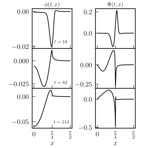
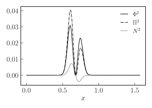
Beginning with weak-field initial data, all of our simulations are consistent with the notion that black holes can form for initial data (47) with arbitrarily small amplitudes $\epsilon$. In Figs. 1-3 we focus on simulations starting from (47) with $\epsilon=6\sqrt{2}$, which bounces off of the AdS boundary 42 times before forming a horizon. We find evidence of the transfer of energy to shorter scales long before the formation of the final black hole. In Fig. 1, we show the scalar field profile from a simulation with $\xi=\frac{1}{6}$. One can see that the $\phi$ profile, which is characterized at early times by a negative lobe and a positive one, slowly transfers energy from the former to the latter. In particular, the outer edge of the positive lobe forms a very sharp jump, which indicates the that energy is concentrated near that point. The formation of a sharp feature is picked up by the spatial gradient of the scalar field, $\Phi$, which exhibits secular growth near the jump in $\phi$ at $x\sim\frac{\pi}{4}$.

The growth of gradients is shown for various values of $\xi$ in Fig. 2 from simulations starting from initial data (47) with $\epsilon=6\sqrt{2}$. Three different metrics are shown: the growth of $\Pi^{2}$, roughly showing the enhancement of $\dot{\phi}$ with each successive bounce, as well as the magnitudes of the Jordan-frame Ricci and Kretschmann scalars, all evaluated at the origin of spherical symmetry. As is discussed in [4], the continuous profile (for example, $\Pi^{2}(t,0)$) takes a complicated form at late times, with many rapid oscillations, so we only show a single point corresponding to the maximum value of each quantity achieved in a cycle of the scalar field imploding through the origin. The figure shows that all of the aforementioned quantities grow at roughly the same rate as a function of the coupling constant, though it is clear that the extent to which this growth is monotonic is affected by the choice of $\xi$. In particular, it seems that the cases with $\xi=0,\frac{1}{6}$ grow roughly monotonically at late times, whereas $\xi=-0.2,-0.1,0.1$ all develop nontrivial patterns of local maxima and minima. The case $\xi=0.18$, somewhat near the BF bound $\xi=0.1875$, (30), shows a pronounced oscillation pattern superimposed over the secular growth of $\Pi^{2},R,K$. Overlaid on each panel in plus-shaped markers are the same results except for simulations with the equivalent mass (29) and a minimal coupling $\xi=0$. The massive, minimally-coupled results are effectively identical to those with the non-minimal coupling until late times (within a few bounces of collapse), indicating that the aforementioned growth of gradients is indeed occurring in the weak-field regime where the nonminimal coupling acts like a mass term in the scalar wave equation (29, 33).

Figure 2: Comparison of three Jordan-frame diagnostics—$\Pi^{2},|R|,|K|$ evaluated at the origin—for different values of $\xi$ for simulations starting from initial data (47) with $\epsilon=6\sqrt{2}$, shown in dots. For the sake of comparison, the same diagnostics are overlaid in with the same colors except with cross-shaped markers for simulations with a minimal coupling $\xi=0$ but equivalent mass as given by (29), e.g. in the top-left panel the dots represent $\Pi^{2},|R|,|K|$ from a simulation with $\xi=-0.2$, and the crosses are $\Pi^{2},|R|,|K|$ from a simulation with $\xi=0,m^{2}=2.4$. For $\xi=0$, the dot and cross simulations are identical, so the crosses are omitted. As in [4], $f(t,0)$ above traces out a continuous curve in each case above, but we plot only the peak value achieved in each implosion through the origin to de-clutter the figure. Note that the growth of $f(t,0)$ is always non-monotonic for $\xi=-0.2,-0.1,0.1,0.18$, but is monotonic after an early nearly growth-free phase for the two special cases $\xi=0,\xi=\frac{1}{6}$. Note also that for $\xi=\frac{1}{6}$, $R$ is constant; see (6).

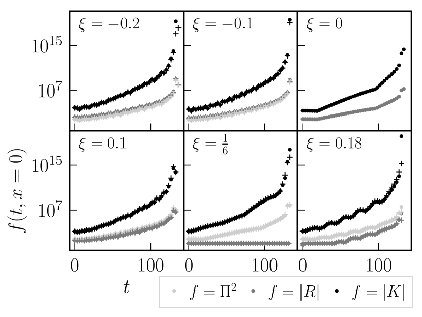
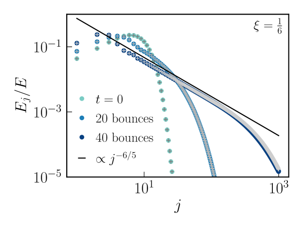
Fig. 3 shows the energy (37) of the solution projected onto the orthonormal basis of solutions to the linearized wave equation on a fixed $AdS_{4}$ background (34). It turns out that the rate of energy transfer is effectively identical for various values of $\xi\in[-0.2,0.18]$, so only a single case ($\xi=\frac{1}{6}$) is shown. Again, overlaid in plus-shaped markers are the same results except for a minimally-coupled massive scalar field with mass given by (29) corresponding to $\xi=\frac{1}{6}$. At early times, the projection of the solution onto modes with high indices $j$ (corresponding to $e_{j}$ with rapid oscillations in $x$) are exponentially suppressed. As time goes on, these modes get populated and the exponential decay is replaced by a power-law with slope $\approx-6/5$, in agreement with that found in [31]. The population of high-$j$ modes is cut off by the formation of an apparent horizon after 42 bounces, only shortly later than the latest time (darkest blue dots) shown in Fig. 3.

Figure 3: Energy per linearized mode $E_{j}$ (34) as a function of $j$ for a simulation with $\xi=\frac{1}{6}$, $\epsilon=6\sqrt{2}$ in blue dots. Also included are points from a simulation with $\xi=0$ and the analogous mass given by (29), namely $m^{2}=-2$, in gray plus signs. The solution shows that at early times, only low-$j$ modes are populated and higher $j$ modes are exponentially suppressed. As time passes, energy is transferred to the higher $j$ modes, and at late times (a couple bounces before horizon formation) a set of these higher $j$ modes follow a power law $\propto j^{-6/5}$ before exponentially decaying at very high $j$ (see [24]). Here $\xi=\frac{1}{6}$ is chosen as a representative case; for $\xi=-0.2,-0.1,0,0.1,0.18$ the figure is essentially identical.

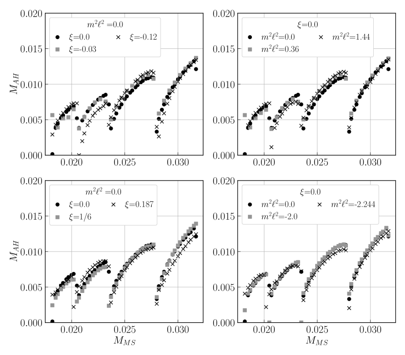
We next consder strong-field initial data, which collapse to a black hole after only a few bounces off the AdS boundary, and focus on the formation of the apparent horizon. In Fig. 4 we compare the mass enclosed in the initial apparent horizon (AH), $M_{AH}$, that forms and the total Misner-Sharp mass of the spacetime $M_{MS}$ (see Sec. 3.3) for Gaussian initial data for different values of $\xi$ and for a massive minimally coupled scalar field with mass $m^{2}=m_{eff}^{2}$. In this figure, it is clear that the AH mass is not monotonic with the total mass of the spacetime; instead, one sees a set of four finger-like clusters which are monotonic in $M_{MS}$, with sudden jumps in $M_{AH}$ in between them. Each finger corresponds to (from right to left) cases which collapse after zero, one, two, and three bounces of the scalar field off of the AdS boundary. We find that the initial data (47) eventually forms apparent horizons in a qualitatively similar way for nonminimally coupled scalar fields as is seen for minimally coupled fields [4]. The masses of the initial apparent horizons are not dramatically affected by the nonminimal coupling nor by a nonzero mass term with $\xi=0$ when compared against those for a minimally coupled, massless field.

Figure 4: Mass of the initial apparent horizon $M_{AH}$ versus the total mass of the spacetime $M_{MS}$ (see Sec. 3.3) for Gaussian initial data (47), where all masses are evaluated in the Jordan frame. The left panels show how the black hole mass changes for a massless nonminimally coupled scalar field. The right panels show how the black hole mass changes for a minimally coupled massive scalar field, where the masses are chosen to agree with the effective masses (29) of the cases in the left panels. The finger-like structures correspond to (from right to left) solutions which bounce zero, one, two, and three times off of the AdS boundary before forming an apparent horizon.

5 The scalar field-viscous fluid analogy

There is a formal analogy between the stress-energy tensor of a minimally coupled scalar field and that of a perfect fluid [41, 42]. This analogy can be made rigorous for irrotational barotropic fluids, where the relativistic Euler equations can be rewritten exactly as a scalar wave equation for a suitably defined scalar field [43, 44], but often in other contexts a scalar field is used for the matter model and the results are interpreted by analogy to a fluid (see, e.g. [45, 46, 47] in the context of inflationary cosmology). We adopt the latter approach here, except with the modification that the nonminimal coupling term in the action (1) results in the presence of terms in the stress-energy tensor (4) which map to viscous corrections to the relativistic fluid [48, 49].

The fact that the nonminimal coupling parameter $\xi$ introduces terms which act as an effective viscosity in the fluid analog is of particular interest when considering the “weakly turbulent” instability of AdS spacetimes, where black holes are formed from weak initial data through the transfer of energy to small scales. If the scalar field is indeed acting as an effective viscous fluid, one might expect the effective viscosity introduced by $\xi$ to combat the transfer of energy to small scales, perhaps slowing or even halting the formation of a black hole. In this section we first briefly review the scalar field-fluid analogy, evaluate the extent to which the scalar field actually behaves as a fluid in our numerical solutions, and show that the scalar’s effective viscosity does not noticeably alter the qualitative features of the solutions.

To derive the scalar field-fluid analogy, we first decompose the stress-energy tensor (assumed only to be a symmetric two-tensor) with respect to a unit timelike four-vector $u^{a}$, and then write it as [50, 51]

$$T^{ab}=\mathcal{E}u^{a}u^{b}+\mathcal{P}\Delta^{ab}+\mathcal{Q}^{a}u^{b}+\mathcal{Q}^{b}u^{a}+\mathcal{T}^{ab},$$ (48)

where

$$\mathcal{E}\equiv u_{a}u_{b}T^{ab},~{}~{}~{}\mathcal{P}\equiv\frac{1}{3}\Delta_{ab}T^{ab},~{}~{}~{}\mathcal{Q}^{a}\equiv-\Delta^{ab}u^{c}T_{bc}$$

$$\mathcal{T}^{ab}\equiv T^{<ab>}\equiv\frac{1}{2}\Big{(}\Delta^{ac}\Delta^{bd}+\Delta^{ad}\Delta^{bc}-\frac{2}{3}\Delta^{ab}\Delta^{cd}\Big{)}T_{cd},$$ (49)

$$\Delta^{ab}\equiv g^{ab}+u^{a}u^{b}.$$

As written, substituting (5) into (48) simply yields the identity $T^{ab}=T^{ab}$. Fluid models are defined by replacing (5) with a set of constitutive relations defining the components $\mathcal{E},\mathcal{P},\mathcal{Q}^{a},\mathcal{T}^{ab}$ in terms of a set of hydrodynamic variables derived from equilibrium thermodynamics, and the four-vector $u^{a}$ is defined to be the (equilibrium) flow velocity of the fluid.

Rather than defining constitutive relations, we instead notice that for a fluid model, $\mathcal{E}$ plays the role of the energy density, $\mathcal{P}$ is the pressure, $\mathcal{Q}^{a}$ is the heat flux vector, and $\mathcal{T}^{ab}$ incorporates the effects of shear viscosity. Though in principle all of the aforementioned terms can acquire non-equilibrium (dissipative) corrections, $\mathcal{Q}^{a}$ and $\mathcal{T}^{ab}$ model purely non-equilibrium effects, and thus vanish for a fluid in equilibrium (see e.g. [51]). Constructing the “fluid analog” of a given non-fluid stress-energy tensor then consists of taking the projections (5) and interpreting them as the energy density, pressure, heat flux, and shear viscosity of a relativistic fluid.

In order to perform the decomposition (48-5) for the scalar-tensor theory (4-5), one must define a timelike unit four-vector to identify with the flow velocity of the fluid. The usual definition [48],

$$u^{a}\equiv\frac{\nabla^{a}\phi}{\sqrt{-\nabla_{c}\phi\nabla^{c}\phi}}\equiv\frac{\nabla^{a}\phi}{N},$$ (50)

is well-defined so long as the gradient of the scalar field remains timelike. One can now perform the decomposition by taking the projections (5), which yields

$$\mathcal{E}_{s} =\frac{1}{1-\kappa\xi\phi^{2}}\Big{(}\frac{1}{2}N^{2}+\frac{\Lambda}{\kappa}-2\xi N\phi\nabla_{b}u^{b}\Big{)}$$ (51)

$$\mathcal{P}_{s} =\frac{1}{1-\kappa\xi\phi^{2}}\Big{(}\frac{1}{2}N^{2}-\frac{\Lambda}{\kappa}+2\xi\Big{[}\phi u^{c}\nabla_{c}N+\frac{2}{3}\phi N\nabla_{c}u^{c}-N^{2}\Big{]}\Big{)}$$ (52)

$$\mathcal{Q}^{a}_{s} =\frac{2\xi N\phi}{1-\kappa\xi\phi^{2}}\,u^{c}\nabla_{c}u^{a}$$ (53)

$$\mathcal{T}^{ab}_{s} =-2\frac{\xi N\phi}{1-\kappa\xi\phi^{2}}\,\sigma^{ab},$$ (54)

where $\sigma^{ab}=\nabla^{<a}u^{b>}$ (see (5)) and each component is given a subscript $s$ to denote that it is derived from the scalar field stress-energy tensor (4-5). We see that the nonminimal coupling adds corrections to $\mathcal{E},\mathcal{P}$, but most significantly makes the effective heat flow vector and shear viscosity nonzero. In this sense, the effects of the nonminimal coupling $\xi\neq 0$ map onto non-equilibrium (viscous) effects in the analog fluid.

Ultimately, we find that the viscous fluid analogy is only of limited use in understanding our results. Computing $N^{2}$ in the coordinate basis used in our simulations, we find

$$N^{2}=\Omega^{2}\frac{\cos^{2}x}{\ell^{2}}\hat{A}\,\big{(}\Pi^{2}-\Phi^{2}\big{)},$$ (55)

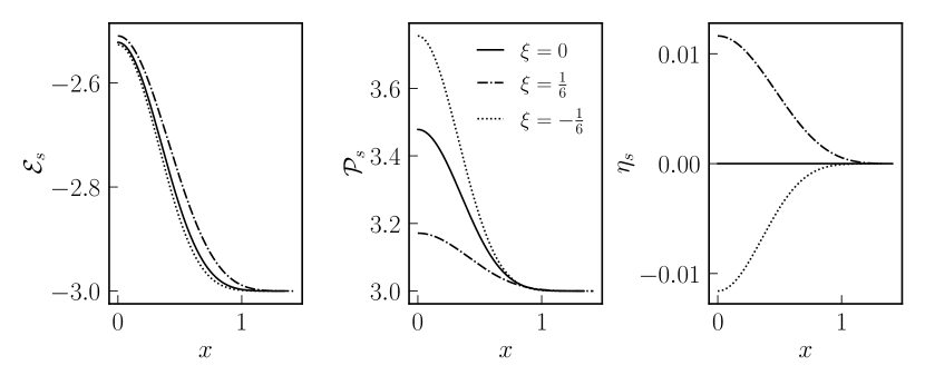
which is negative if $\Phi^{2}>\Pi^{2}$. The effective four-velocity is almost never timelike across the entire spatial domain due to the fact that $\Pi$ decays faster than $\Phi$ approaching the AdS boundary ($\Phi\sim\rho^{\Delta-1},\Pi\sim\rho^{\Delta}$, see (2.3)). Since $\Delta\geq 3/2>0$, we expect that the fluid interpretation can only be valid across the entire spatial domain when $\Phi$ is compactly supported away from the AdS boundary. Fig. 5 shows $\Phi^{2},\Pi^{2}$, and $N^{2}$ for an evolution starting from Gaussian initial data (47) with $\epsilon=10$ at a point in time when the field is concentrated in the center of the domain—note that $N^{2}$ is negative from $x\sim 0.75$ all the way to the outer boundary $x=\frac{\pi}{2}$.

Figure 5: Snapshot from an evolution starting from Gaussian initial data (47) with $\epsilon=10$, at a time when the field is concentrated near the center of the domain. Note that $\Phi^{2}>\Pi^{2}$ over the entire region $x\raisebox{-3.69899pt}{~{}\shortstack{$>$ \\ [-0.07cm]$\sim$}}~{}0.75$, implying the four-vector identified with the flow velocity in the fluid analogy (50) is spacelike rather than timelike.

That said, in the weak-field limit ($\phi\ll 1$) the mode solutions (34) are time-periodic and will, at times, have $\Phi=0\,\forall\,x$. We show the components $\mathcal{E}_{s},\mathcal{P}_{s}$ (51-52) as well as the effective shear viscosity (defined by comparison of $\mathcal{T}^{ab}=-2\eta\sigma^{ab}$ to (54) for the viscous fluid [51])

$$\eta_{s}\equiv\frac{\xi N\phi}{1-\kappa\xi\phi^{2}},$$ (56)

of the fluid analog from an evolution with initial data based on the $n=0$ mode of (34), namely

$$\phi(0,x)=0,~{}~{}~{}\Phi(0,x)=0,~{}~{}~{}\Pi(0,x)=\epsilon\cos(x)^{\Delta}$$ (57)

with $\epsilon=1$ at a time when $u^{a}$ (50) is timelike everywhere in Fig 6. Even at times when the fluid analog is well-defined (i.e. where $u^{a}$ is timelike), we find that the total energy density is negative ($\mathcal{E}_{s}<0$)—which signals a violation of the weak energy condition for an observer co-moving with the “fluid”—and the effective shear viscosity changes sign with the scalar field, periodically attaining unphysical negative values.

Figure 6: Components of the fluid analog (51-54) from an evolution starting from mode-0 initial data (34) of the form (57) with $\epsilon=1$, at a time when the four-vector $u^{a}$ (50) is timelike almost everywhere. Shown in the three panels are the total energy density seen by a co-moving observer $\mathcal{E}_{s}$ (51), the pressure $\mathcal{P}_{s}$ (52), and the effective shear viscosity $\eta_{s}$ (56), for scalar fields with $\xi=0,\frac{1}{6},-\frac{1}{6}$. Note that the energy density is negative, which is unphysical and amounts to a violation of the weak energy condition. The pressure is positive, as expected, and seems to be enhanced for $\xi<0$ and diminished for $\xi>0$. The effective shear viscosity changes sign during the evolution, and the sign at a given time is determined by the sign of the product $\xi\phi$ (56).

In summary, the scalar field-viscous fluid analogy is not of much utility for the case considered here, as the quantity typically identified with the effective fluid’s four-velocity (50) does not remain timelike in the presence of significant spatial anisotropy. For the case shown here when the analog is well-defined, the effective fluid displays a negative energy density and the shear viscosity changes sign in time. Similar effects were seen in [52], though they find reasonable behavior when defining certain thermodynamic quantities (such as the temperature). We find that the effective viscosity (56) does not inhibit (or enhance) the weakly turbulent instability of $AdS_{4}$ spacetime in our simulations.

6 Discussion

In this study we have numerically investigated the instability of asymptotically $AdS_{4}$ spacetimes for a nonminimally coupled scalar field model. We find that the qualitative behavior of our solutions do not differ from those of minimally coupled massive and massless scalar fields: from small “generic” initial scalar field perturbations, energy is transferred over time to increasingly smaller scales, until a black hole is formed. While we work in the Einstein frame of the theory, where the nonminimal coupling is absorbed into the metric via a Weyl rescaling, we measure the formation of black holes and the transfer of energy in the Jordan frame, where the scalar field couples directly to the Ricci scalar.

Our work does not address the stability of black holes in the theory we consider. In the Jordan frame, the theory in principle allows for violations of the NCC, which underlies the classical black hole area theorem [33]. It would be interesting to consider the stability of asymptotically AdS spacetime in horizon-penetrating coordinates, as one would then be able to evolve the dynamics of the solution beyond apparent horizon formation to determine if it is eventually enveloped by an event horizon. Critical collapse solutions have been studied for nonminimally coupled scalar fields in asymptotically flat spacetimes [53], although not to our knowledge for asymptotically AdS spacetimes; it would be interesting to determine the effect (if any) of the cosmological constant on such critical collapse solutions. We leave to future work a more thorough study of the dynamics of collapse for values of $\xi$ very close to the Breitenlohner-Freedman bound ($\xi=\frac{3}{16}=0.1875$). While we were able to perform numerical evolutions of $\xi$ somewhat near the bound (up to $\xi=0.187$), it would be interesting to determine the behavior of solutions for theories which saturate that bound.

In Sec. 5 we considered the interpretation of the scalar field’s stress-energy tensor as that of a relativistic viscous fluid. This analogy is of particular interest here, as one could conjecture that the viscosity in the fluid analog (which is introduced by the nonminimal coupling $\xi$) would hamper the transfer of energy to small scales characterizing the AdS instability. Unfortunately the analogy breaks down in the case of interest, as it is only applicable when the gradient of the scalar field is timelike, which generically is not the case in parts of the domain due to spatial anisotropy in the field configuration. That said, the question of whether or not true physical viscosity inhibits the instability of AdS is an open question, and it may be addressed using a legitimate relativistic viscous fluid theory such as, for example, Müller-Israel-Stewart theory [54, 55, 56] or Bemfica-Disconzi-Noronha-Kovtun theory [57, 58]. In such a study, the presence of viscosity should combat the gradient-sharpening effect of the AdS instability, and it would be quite interesting to determine which effect wins out as a function of the “amount” of viscosity in the model. In principle, there are three possibilities: (1) an infinitesimal amount of viscosity makes AdS spacetime stable to small enough perturbations (it adds a “mass gap” to the black holes that form from perturbative initial data); (2) a finite amount of viscosity is required for stability, in which case the threshold would be interesting to investigate; or (3) viscosity has no impact on or only slows the growth of gradients and horizons still form. The answer to this question would further elucidate the structure of the instability, and would also serve to clarify the relationship between AdS “turbulence” and that experienced in fluid flows.

Appendix A Numerical methods and convergence tests

We solve the evolution equations (21), (25), the constraint equations (19) and (20), and the spatial derivative of (25):

$$\dot{\Phi}=\left(\hat{A}e^{-\hat{\delta}}\Pi\right)^{\prime},$$ (58)

using finite difference methods. We evolve $\phi,\Phi,\Pi$ in time using the method of lines with the standard fourth-order Runge-Kutta method, and use fourth-order finite difference stencils to approximate spatial derivatives.

As is described in [4, 31], the main challenge in solving these equations lies in maintaining stability at the origin and at the AdS boundary. To help maintain stability, following [24] we rescale the scalar field and its derivatives via

$$\tilde{\phi}\equiv \frac{1}{\cos^{\Delta-1}x}\phi,$$ (59)

$$\tilde{\Pi}\equiv \frac{1}{\cos^{\Delta-1}x}\Pi,$$ (60)

$$\tilde{\Phi}\equiv \frac{1}{\cos^{\Delta-2}x}\Phi,$$ (61)

and these variables are evolved rather than $\phi,\Phi,\Pi$. This is done because the fields $\phi,\Phi,\Pi$ decay at rates inversely proportional to $\xi$ approaching the AdS boundary, implying larger field values near $x=\frac{\pi}{2}$ for large $\xi$ than for small $\xi$; this, in turn, results in a loss of stability for $\xi>0$. The rescaled fields always have the falloff $\tilde{\phi},\tilde{\Pi},\tilde{\Phi}\sim\rho$, resulting in significantly improved stability for $\xi>0$. The definitions (59), when combined with the falloff behavior (2.3), (2.3) implies the boundary conditions

$$\phi^{\prime}(0)=\Phi(0)=\Pi^{\prime}(0)=0$$ (62)

$$\phi\Big{(}\frac{\pi}{2}\Big{)}=\Phi\Big{(}\frac{\pi}{2}\Big{)}=\Pi\Big{(}\frac{\pi}{2}\Big{)}=0.$$ (63)

Rather than using forward- or backward-biased finite difference stencils near the origin and AdS boundary respectively, we use a fourth-order centered stencil and set the field values lying outside of the domain using the parity of the field at the boundary: namely, $\phi,\Pi$ are even and $\Phi$ is odd at the origin, and $\phi,\Phi,\Pi$ are all odd at the outer boundary. This means that if a stencil requires fields at a point $-x_{i}<0$, for example, then $\phi(-x_{i})=\phi(x_{i})$, $\Pi(-x_{i})=\Pi(x_{i})$, and $\Phi(-x_{i})=-\Phi(x_{i})$; for points $x_{i}>\frac{\pi}{2}$, the odd parity of the fields $f\in\{\phi,\Phi,\Pi\}$ implies $f(\frac{\pi}{2}-x_{i})=-f(\frac{\pi}{2}+x_{i})$.

It turns out that, even with fourth-order spatial derivative stencils, the truncation error in the $\Pi$ evolution equation (21) is large enough near the origin and the AdS boundary to destabilize the numerical scheme. Thus, instead of solving (21) at the first and last interior gridpoints—i.e. the gridpoint adjacent to the gridpoint at the origin and the gridpoint adjacent to the gridpoint at the AdS boundary—we use cubic spline interpolation to set the value of $\Pi$. A “natural cubic spline” gives an interpolated value of a function $f$ at position $x$ using values of $f$ and its derivatives at so-called knot points $x_{i},x_{j}$ (where $x_{i}\leq x\leq x_{j}$) [59]:

$$f(x)=\frac{(x_{j}-x)^{3}f^{\prime\prime}(x_{i})+(x-x_{i})^{3}f^{\prime\prime}(x_{j})}{6(x_{j}-x_{i})}+\frac{(x_{j}-x)f(x_{i})+(x-x_{i})f(x_{j})}{x_{j}-x_{i}}$$

$$-\frac{1}{6}\left(x_{j}-x_{i}\right)\left[\left(x_{j}-x\right)f^{\prime\prime}(x_{i})+\left(x-x_{i}\right)f^{\prime\prime}(x_{j})\right],$$ (64)

where in this case we take $f=\Pi$, $x=x_{1}$, $x_{i}=x_{0}$, and $x_{j}=x_{2}$. The second derivative terms $\Pi^{\prime\prime}$ are computed using fourth-order centered finite difference stencils, making use of the parity of $\Pi$ to set field values when the stencil extends past the boundary of the domain.

Spline interpolation (A) turns out to be especially effective at damping spurious numerical oscillations, and as a result is essential to the stability of solutions which have many bounces off of the boundaries (such as the 42-bounce data shown in Fig. 2, and the many-bounce evolutions shown in [4, 31]). For these simulations, the standard fourth-order Runge-Kutta method is used to integrate the constraint equations (19) and (20). This method requires values of the fields in between spatial gridpoints (at locations $x_{k+\frac{1}{2}}$), so we use natural cubic spline interpolation (A) with $x=x_{k+\frac{1}{2}}$, $x_{i}=x_{k}$, and $x_{j}=x_{k+1}$. For the study of apparent horizon formation (Fig. 4), the simulations of interest form apparent horizons within only a couple of bounces, so a simpler second-order Runge-Kutta method is used to integrate the constraint equations; this method does not require field values at half-gridpoints, so cubic spline interpolation is only used for $\Pi$ at the gridpoints near the inner and outer boundaries. This being said, we were unable to stably numerically evolve simulations for values of $\xi$ that saturate the BF bound, $\xi=3/16$.

To solve the constraints, we integrate (20) for $\hat{\delta}$ inward from the AdS boundary to the origin. We solve for $\hat{A}$ by first defining the Einstein frame Misner-Sharp mass function [24]

$$1-\frac{2\hat{M}_{MS}(t,x)}{\hat{R}_{area}}-\frac{1}{3}\hat{R}_{area}^{2}\Lambda=\hat{g}^{ab}\hat{\nabla}_{a}\hat{R}_{area}\hat{\nabla}_{b}\hat{R}_{area},$$ (65)

where $\hat{R}_{area}=\ell\tan x$. Substituting for $\hat{R}$, from Eq. (65) we find that

$$\hat{A}\left(t,x\right)=1-2\frac{\cos^{3}x}{\sin x}\frac{\hat{M}_{MS}\left(t,x\right)}{\ell},$$ (66)

where our definition for the Einstein frame Misner-Sharp mass differs from that of Buchel et. al. [24] by a factor of $2/\ell$. Using (66), the constraint (19) then becomes

$$\hat{M}_{MS}^{\prime}=\frac{\kappa\ell}{2}\frac{\sin^{2}x}{\cos^{2}x}\left(\frac{1}{2}\left[\Pi^{2}+\Phi^{2}\right]\left[1-2\frac{\cos^{3}}{\sin x}\frac{\hat{M}_{MS}}{\ell}\right]q\left(\phi\right)-\frac{3\xi}{\cos^{2}x}\;z\left(\phi\right)\right).$$ (67)

We integrate this expression rather than (19), as doing so results in significantly improved numerical stability; we then apply (65) to recover $\hat{A}$.

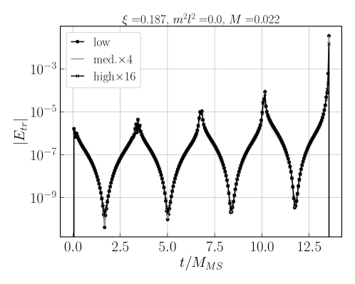
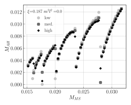
To check the convergence of our code, we evaluated the equation for $\dot{\hat{A}}$, Eq. (22), which is unused by our solution algorithm, and verified that it goes to zero with higher resolution at a rate consistent with the accuracy of the numerical scheme used. We plot a representative convergence test in Fig. 7 for a run that had three bounces, $\xi=0.187$, and total Misner-Sharp mass of $0.022$. We find that the independent residual goes to zero at the expected rate for a scheme which is second-order in the grid spacing, in accordance with the fact that the scheme used solves the constraint equations (19-20) using a second-order Runge-Kutta integrator. In Fig. 8 we show that the apparent horizon mass does not vary significantly with numerical resolution for evolutions with $\xi=0.187$ (the least numerically stable case we consider), implying that the dynamics are sufficiently converged at the resolutions used.

Figure 7: Plot of the one norm of the independent residual (22), which we denote by the “$tr$” component of the Einstein equations, $E_{tr}$. The “low” resolution corresponds to $2^{12}$ radial grid points, and the “med.” and “high” resolutions have twice and four times that base grid resolution. We rescale the one-norm by $4$ and $16$ in the plot, which shows second-order convergence, which is consistent with the stencils we used in our code to compute the constraint equations. Here $M_{MS}$ is the total Misner-Sharp mass of the spacetime.

Figure 8: Misner-Sharp mass of the first apparent horizon versus the total Misner-Sharp mass. We see that we are able to resolve the formation of apparent horizons for the range of initial data we considered. The “low” resolution run has $2^{12}$ radial grid points, while the “med.” and “high” runs have twice and four times that resolution. The scatter in the grid points near the boundaries between the finger-like clusters indicates the difficulty in resolving the masses of very small black holes. The data presented in Fig. 4 were run at the “high” resolution.

Appendix B Jordan-frame Kretschmann scalar

As a diagnostic we compute the Kretschmann scalar $K\equiv R_{abcd}R^{abcd}$ derived from the Jordan frame metric (31). We only use $K$ at the origin of the spherically symmetric spacetime, which is

$$K(t,0)=\frac{1}{l^{4}\left(1-\kappa\xi\phi^{2}\right)^{2}}\Bigg{(}4\kappa^{3}\xi^{3}\phi^{6}\Big{(}-\hat{A}^{\prime\prime 2}-e^{2\hat{\delta}}\kappa\xi\left(\dot{\phi}^{2}(\hat{A}^{\prime\prime}-2\hat{\delta}^{\prime\prime}+10)+2\dot{\hat{\delta}}\dot{\phi}\phi^{\prime\prime}+2\ddot{\phi}\phi^{\prime\prime}\right)$$

$$+4\hat{A}^{\prime\prime}\hat{\delta}^{\prime\prime}-4\hat{A}^{\prime\prime}+3e^{4\hat{\delta}}\kappa\xi(\dot{\hat{\delta}}\dot{\phi}+\ddot{\phi})^{2}-4\hat{\delta}^{\prime\prime 2}+8\hat{\delta}^{\prime\prime}+3\kappa\xi\phi^{\prime\prime 2}-20\Big{)}$$

$$+2\kappa^{2}\xi^{2}\phi^{4}\Big{(}3\hat{A}^{\prime\prime 2}+2\hat{A}^{\prime\prime}\left(e^{2\hat{\delta}}\kappa\xi\dot{\phi}^{2}-6\hat{\delta}^{\prime\prime}+6\right)$$

$$+4\kappa\xi\left(2e^{2\hat{\delta}}\phi^{\prime\prime}(\dot{\hat{\delta}}\dot{\phi}+\ddot{\phi})-3e^{4\hat{\delta}}(\dot{\hat{\delta}}\dot{\phi}+\ddot{\phi})^{2}+e^{2\hat{\delta}}\dot{\phi}^{2}\left(3e^{2\hat{\delta}}\kappa\xi\dot{\phi}^{2}-\hat{\delta}^{\prime\prime}+7\right)-3\phi^{\prime\prime 2}\right)+12((\hat{\delta}^{\prime\prime}-2)\hat{\delta}^{\prime\prime}+5)\Big{)}$$

$$+4\kappa\xi\phi^{2}\Big{(}-\hat{A}^{\prime\prime 2}+\hat{A}^{\prime\prime}\left(e^{2\hat{\delta}}\kappa\xi\dot{\phi}^{2}+4\hat{\delta}^{\prime\prime}-4\right)$$

$$+\kappa\xi\left(-2e^{2\hat{\delta}}\phi^{\prime\prime}(\dot{\hat{\delta}}\dot{\phi}+\ddot{\phi})+3e^{4\hat{\delta}}(\dot{\hat{\delta}}\dot{\phi}+\ddot{\phi})^{2}+2e^{2\hat{\delta}}\dot{\phi}^{2}\left(3e^{2\hat{\delta}}\kappa\xi\dot{\phi}^{2}-\hat{\delta}^{\prime\prime}+1\right)+3\phi^{\prime\prime 2}\right)-4((\hat{\delta}^{\prime\prime}-2)\hat{\delta}^{\prime\prime}+5)\Big{)}$$

$$+\kappa^{4}\xi^{4}\phi^{8}\left(\hat{A}^{\prime\prime 2}-4(\hat{A}^{\prime\prime}+2)\hat{\delta}^{\prime\prime}+4\hat{A}^{\prime\prime}+4\hat{\delta}^{\prime\prime 2}+20\right)$$

$$-12\kappa^{3}\xi^{3}\phi^{5}\left(e^{2\hat{\delta}}(\dot{\hat{\delta}}\dot{\phi}+\ddot{\phi})-\phi^{\prime\prime}\right)\left(\hat{A}^{\prime\prime}+2e^{2\hat{\delta}}\kappa\xi\dot{\phi}^{2}-2\hat{\delta}^{\prime\prime}+6\right)$$

$$+4\kappa^{2}\xi^{2}\phi^{3}\left(e^{2\hat{\delta}}\left(3(\hat{A}^{\prime\prime}-2\hat{\delta}^{\prime\prime}+6)(\dot{\hat{\delta}}\dot{\phi}+\ddot{\phi})-4\kappa\xi\dot{\phi}^{2}\phi^{\prime\prime}\right)-3\phi^{\prime\prime}(\hat{A}^{\prime\prime}-2\hat{\delta}^{\prime\prime}+6)\right)$$

$$-4\kappa^{4}\xi^{4}\phi^{7}(\hat{A}^{\prime\prime}-2\hat{\delta}^{\prime\prime}+6)\left(\phi^{\prime\prime}-e^{2\hat{\delta}}(\dot{\hat{\delta}}\dot{\phi}+\ddot{\phi})\right)$$

$$+4\kappa\xi\phi\left(e^{2\hat{\delta}}(\dot{\hat{\delta}}\dot{\phi}+\ddot{\phi})\left(-\hat{A}^{\prime\prime}+6e^{2\hat{\delta}}\kappa\xi\dot{\phi}^{2}+2\hat{\delta}^{\prime\prime}-6\right)+\phi^{\prime\prime}\left(\hat{A}^{\prime\prime}-2\left(e^{2\hat{\delta}}\kappa\xi\dot{\phi}^{2}+\hat{\delta}^{\prime\prime}-3\right)\right)\right)$$

$$-4e^{2\hat{\delta}}\kappa\xi\dot{\phi}^{2}(\hat{A}^{\prime\prime}-2\hat{\delta}^{\prime\prime}+6)+(\hat{A}^{\prime\prime}-2\hat{\delta}^{\prime\prime})^{2}+4(\hat{A}^{\prime\prime}-2\hat{\delta}^{\prime\prime}+5)+12e^{4\hat{\delta}}\kappa^{2}\xi^{2}\dot{\phi}^{4}\Bigg{)}.$$ (68)

References

- [1] Friedrich H 1986 Communications in Mathematical Physics 107 587–609 ISSN 1432-0916 URL https://doi.org/10.1007/BF01205488
- [2] Christodoulou D and Klainerman S 1993 The Global Nonlinear Stability of the Minkowski Space (PMS-41) (Princeton University Press) URL http://www.jstor.org/stable/j.ctt7zthns
- [3] Dafermos M and Holzegel G 200 https://www.dpmms.cam.ac.uk/~md384/ADSinstability.pdf URL https://www.dpmms.cam.ac.uk/~md384/ADSinstability.pdf
- [4] Bizon P and Rostworowski A 2011 Phys. Rev. Lett. 107 031102 (Preprint 1104.3702)
- [5] Buchel A, Liebling S L and Lehner L 2013 Phys. Rev. D 87 123006 (Preprint 1304.4166)
- [6] Balasubramanian V, Buchel A, Green S R, Lehner L and Liebling S L 2014 Phys. Rev. Lett. 113 071601 (Preprint 1403.6471)
- [7] Bizoń P 2014 Gen. Rel. Grav. 46 1724 (Preprint 1312.5544)
- [8] Evnin O 2021 Class. Quant. Grav. 38 203001 (Preprint 2104.09797)
- [9] Bantilan H, Figueras P, Kunesch M and Romatschke P 2017 Phys. Rev. Lett. 119 191103 (Preprint 1706.04199)
- [10] Bantilan H, Figueras P and Rossi L 2021 Phys. Rev. D 103 086006 (Preprint 2011.12970)
- [11] Dias O J C, Horowitz G T and Santos J E 2012 Class. Quant. Grav. 29 194002 (Preprint 1109.1825)
- [12] Craps B, Evnin O and Vanhoof J 2014 JHEP 10 048 (Preprint 1407.6273)
- [13] Bizoń P, Maliborski M and Rostworowski A 2015 Phys. Rev. Lett. 115 081103 (Preprint 1506.03519)
- [14] Moschidis G 2020 Anal. Part. Diff. Eq. 13 1671–1754 (Preprint 1704.08681)
- [15] Moschidis G 2018 (Preprint 1812.04268)
- [16] Ishibashi A and Wald R M 2004 Class. Quant. Grav. 21 2981–3014 (Preprint hep-th/0402184)
- [17] Polchinski J 2007 String theory. Vol. 1: An introduction to the bosonic string Cambridge Monographs on Mathematical Physics (Cambridge University Press) ISBN 978-0-511-25227-3, 978-0-521-67227-6, 978-0-521-63303-1
- [18] Fujii Y and Maeda K i 2003 The Scalar-Tensor Theory of Gravitation Cambridge Monographs on Mathematical Physics (Cambridge University Press)
- [19] Hubeny V E 2015 Class. Quant. Grav. 32 124010 (Preprint 1501.00007)
- [20] Kaiser D I 2010 Physical Review D 81 ISSN 1550-2368 URL http://dx.doi.org/10.1103/PhysRevD.81.084044
- [21] Winstanley E 2002 On the existence of conformally coupled scalar field hair for black holes in (anti-)de sitter space (Preprint gr-qc/0205092)
- [22] Faraoni V, Gunzig E and Nardone P 1999 Fund. Cosmic Phys. 20 121 (Preprint gr-qc/9811047)
- [23] Flanagan E E 2004 Class. Quant. Grav. 21 3817 (Preprint gr-qc/0403063)
- [24] Buchel A, Lehner L and Liebling S L 2012 Phys. Rev. D 86 123011 (Preprint 1210.0890)
- [25] Breitenlohner P and Freedman D Z 1982 Physics Letters B 115 197–201 ISSN 0370-2693 URL https://www.sciencedirect.com/science/article/pii/0370269382906438
- [26] Breitenlohner P and Freedman D Z 1982 Annals of Physics 144 249–281 ISSN 0003-4916 URL https://www.sciencedirect.com/science/article/pii/0003491682901166
- [27] Avis S J, Isham C J and Storey D 1978 Phys. Rev. D 18(10) 3565–3576 URL https://link.aps.org/doi/10.1103/PhysRevD.18.3565
- [28] Fodor G, Forgács P and Grandclément P 2014 Phys. Rev. D 89 065027 (Preprint 1312.7562)
- [29] Fodor G, Forgács P and Grandclément P 2015 Phys. Rev. D 92 025036 (Preprint 1503.07746)
- [30] NIST Digital Library of Mathematical Functions http://dlmf.nist.gov/, Release 1.1.3 of 2021-09-15 f. W. J. Olver, A. B. Olde Daalhuis, D. W. Lozier, B. I. Schneider, R. F. Boisvert, C. W. Clark, B. R. Miller, B. V. Saunders, H. S. Cohl, and M. A. McClain, eds. URL http://dlmf.nist.gov/
- [31] Maliborski M and Rostworowski A 2013 Int. J. Mod. Phys. A 28 1340020 (Preprint 1308.1235)
- [32] Schleich K and Witt D M 2010 Journal of Mathematical Physics 51 112502 ISSN 1089-7658 URL http://dx.doi.org/10.1063/1.3503447
- [33] Hawking S W 1971 Phys. Rev. Lett. 26(21) 1344–1346 URL https://link.aps.org/doi/10.1103/PhysRevLett.26.1344
- [34] Scheel M A, Shapiro S L and Teukolsky S A 1995 Phys. Rev. D 51 4208–4235 (Preprint gr-qc/9411025)
- [35] Scheel M A, Shapiro S L and Teukolsky S A 1995 Phys. Rev. D 51 4236–4249 (Preprint gr-qc/9411026)
- [36] Baumgarte T W and Shapiro S L 2010 Numerical Relativity: Solving Einstein’s Equations on the Computer (Cambridge University Press)
- [37] Misner C W and Sharp D H 1964 Phys. Rev. 136 B571–B576
- [38] Hawking S 1968 J. Math. Phys. 9 598–604
- [39] Hayward S A 1994 Phys. Rev. D 49 831–839 (Preprint gr-qc/9303030)
- [40] Maeda H and Nozawa M 2008 Phys. Rev. D 77 064031 (Preprint 0709.1199)
- [41] Moncrief V 1980 ApJ 235 1038–1046
- [42] Landau L and Lifshitz E 2013 Fluid Mechanics: Landau and Lifshitz: Course of Theoretical Physics, Volume 6 v. 6 (Elsevier Science) ISBN 9781483161044 URL https://books.google.com/books?id=eOBbAwAAQBAJ
- [43] Fajman D, Oliynyk T A and Wyatt Z 2021 Commun. Math. Phys. 383 401–426 (Preprint 2002.02119)
- [44] Rodnianski I and Speck J 2009 (Preprint 0911.5501)
- [45] Aditya Y and Reddy D R K 2019 Astrophys. Space Sci. 364 3
- [46] Trodden M and Carroll S M 2004 TASI lectures: Introduction to cosmology Theoretical Advanced Study Institute in Elementary Particle Physics (TASI 2002): Particle Physics and Cosmology: The Quest for Physics Beyond the Standard Model(s) pp 703–793 (Preprint astro-ph/0401547)
- [47] Liddle A R and Lyth D H 2000 Cosmological Inflation and Large-Scale Structure
- [48] Madsen M S 1988 Class. Quant. Grav. 5 627–639
- [49] Faraoni V 2012 Phys. Rev. D 85 024040 (Preprint 1201.1448)
- [50] Eckart C 1940 Physical Review 58 919–924
- [51] Kovtun P 2012 J. Phys. A 45 473001 (Preprint 1205.5040)
- [52] Faraoni V and Giusti A 2021 Phys. Rev. D 103 L121501 (Preprint 2103.05389)
- [53] Choptuik M W 1992 “Critical” behaviour in massless scalar field collapse (Cambridge University Press) p 202–222
- [54] Müller I 1967 Zeitschrift für Physik 198 329–344 cited By :447 URL www.scopus.com
- [55] Israel W 1976 Annals Phys. 100 310–331
- [56] Israel W and Stewart J 1979 Annals of Physics 118 341 – 372 ISSN 0003-4916 URL http://www.sciencedirect.com/science/article/pii/0003491679901301
- [57] Bemfica F S, Disconzi M M and Noronha J 2022 Phys. Rev. X 12 021044 (Preprint 2009.11388)
- [58] Kovtun P 2019 JHEP 10 034 (Preprint 1907.08191)
- [59] Atkinson K and Han W 2004 Elementary Numerical Analysis (Wiley) ISBN 9780471433378 URL https://books.google.com/books?id=2CQnAQAAIAAJ