General Law of iterated logarithm for Markov processes: Liminf laws

Abstract.

Continuing from [12], in this paper, we discuss general criteria and forms of liminf laws of iterated logarithm (LIL) for continuous-time Markov processes. Under some minimal assumptions, which are weaker than those in [12], we establish liminf LIL at zero (at infinity, respectively) in general metric measure spaces. In particular, our assumptions for liminf law of LIL at zero and the form of liminf LIL are truly local so that we can cover highly space-inhomogenous cases. Our results cover all examples in [12] including random conductance models with long range jumps. Moreover, we show that the general form of liminf law of LIL at zero holds for a large class of jump processes whose jumping measures have logarithmic tails and Feller processes with symbols of varying order which are not covered before.

Keywords: liminf law; jump processes; law of the iterated logarithm; sample path;

MSC 2020: 60J25; 60F15; 60J35; 60J76; 60F20.

1. Introduction and general result

Let $Y:=(Y_{t})_{t\geq 0}$ be a nontrivial strictly $\beta$-stable process on ${\mathbb{R}}^{d}$ with $0<\beta\leq 2$, in the sense of [31, Definition 13.1]. Assume that none of the one dimensional projections of $Y$ is a subordinator, and $Y$ has no drift when $\beta=1$ (namely, $\tau=0$ in [31, (14.16)]). Then $Y$ satisfies the following Chung-type liminf LIL: There exists a constants $C\in(0,\infty)$ such that

$$\liminf_{t\to 0\;\;(\text{resp. }t\to\infty)}\frac{\sup_{0<s\leq t}|Y_{s}|}{(t/\log|\log t|)^{1/\beta}}=C\;\;\mbox{ a.s.}$$ (1)

See, e.g. [31, Chapters 47, 48].

The liminf LIL (1) was established for random walks on ${\mathbb{Z}}$ by Chung [14] under the assumption that their i.i.d. increments have a finite third moment and expectation zero. The liminf LIL in [14] was improved to a finite second moment assumption by Jain and Pruitt [23]. For some related results, we refer to [35, 17, 24]. Chung also showed the large time result of (1) for a Brownian motion in ${\mathbb{R}}$. The liminf LIL has been extended to non-Cauchy $\beta$-stable processes on ${\mathbb{R}}^{d}$ with $\beta<d$ by Taylor [33], increasing random walks and subordinators by Fristedt and Pruitt [18], and symmetric Lévy processes in ${\mathbb{R}}$ by Dupuis [16]. Then Wee [34] succeeded in obtain liminf LILs for numerous non-symmetric Lévy processes in ${\mathbb{R}}$. See also [1, 5] and the references therein. Recently, Knopova and Schilling [27] extended liminf LIL at zero to non-symmetric Lévy-type processes in ${\mathbb{R}}$. Also, very recently, the second named author, jointly with Kumagai and Wang [25] extended liminf LIL for symmetric mixed stable-like Feller processes on metric measure spaces.

The purpose of this paper is to understand asymptotic behaviors of a given Markov process by establishing liminf law of iterated logarithms for both near zero and near infinity under some minimal assumptions. In particular, we introduce new but general version of it. See Theorem 1.2 below. Our assumptions are weak enough so that our results cover a lot of Markov processes including jump processes with diffusion part, jump processes with small jumps of slowly varying intensity, some non-symmetric processes, processes with singular jumping kernels and random conductance models with long range jumps. See the examples in Sections 2-4, and the references therein. In particular, the class of Markov processes considered in this paper extends the results of [25]. Moreover, metric measure spaces in this paper can be random, disconnected and highly space-inhomogeneous (see Definition 1.5).

Throughout this section, Section 5 and Appendix 6, we assume that $(M,d,\mu)$ is a locally compact separable metric measure space where $\mu$ is a positive Radon measure on $M$ with full support. We add a cemetery point $\partial$ to $M$ and denote $M_{\partial}=M\cup\{\partial\}$. We consider a Borel standard Markov process $X=(\Omega,{\cal F}_{t},X_{t},\theta_{t},t\geq 0;{\mathbb{P}}^{x},x\in M_{\partial})$ on $M_{\partial}$ with the lifetime $\zeta:=\inf\{t>0:X_{t}=\partial\}$. Here $(\theta_{t})_{t\geq 0}$ is the shift operator with respect to $X$ which is defined as $X_{s}(\theta_{t}\,\omega)=X_{s+t}(\omega)$ for all $t,s\geq 0$. Since $X$ is a Borel standard process, $X$ has a Lévy system in the sense of [3, Theorem 1.1]. In this paper, we always assume that $X$ admits a Lévy system of the form $(J(x,\cdot),ds)$ so that for any $z\in M$, $t>0$ and nonnegative Borel function $F$ on $M\times M_{\partial}$ vanishing on the diagonal,

$${\mathbb{E}}^{z}\bigg{[}\,\sum_{s\leq t}F(X_{s-},X_{s})\,\bigg{]}={\mathbb{E}}^{z}\left[\int_{0}^{t}\int_{M_{\partial}}F(X_{s},y)J(X_{s},dy)ds\right].$$

The measure $J(x,dy)$ on $M_{\partial}$ is called the Lévy measure of the process $X$. Here we emphasize that the killing term $J(x,\partial)$ is included in the Lévy measure.

For $x\in M$ and $r\in(0,\infty]$, set $B(x,r):=\{y\in M:d(x,y)<r\}$ and $V(x,r):=\mu(B(x,r))$ with a convention $B(x,\infty)=M$. For a subset $U\subset M$, we denote $\updelta_{U}(x)$ for the distance between $x$ and $M\setminus U$, namely,

$$\updelta_{U}(x)=\inf\{d(x,y):y\in M\setminus U\},\quad x\in M.$$

We fix a base point $o\in M$ and define

$${\mathsf{d}}(x)=d(x,o)+1,\quad x\in M.$$

Since ${\mathsf{d}}(x)\geq 1$, the map $\to$ ${\mathsf{d}}(x)^{\upsilon}$ is nondecreasing on $(0,\infty)$.

For a Borel set $D\subset M$, we denote

$$\tau_{D}:=\inf\{t>0:X_{t}\in M_{\partial}\setminus D\}$$

for the first exit time of $X$ from $D$.

We are now ready to introduce our assumptions. Our assumptions are given in terms of mean exit times, tails of Lévy measures and survival probabilities on balls. Our assumptions are weaker than those in [12], see Lemmas 6.4 and 6.5 in Appendix 6.

Here are our assumptions for liminf LIL at zero. Let $U\subset M$ be an open subset of $M$.

There exist constants $R_{0}>0$, $C_{0}\in(0,1)$, $C_{1}>1$, $C_{i}>0$, $2\leq i\leq 7$ such that for every $x\in U$ and $0<r<R_{0}\wedge(C_{0}\updelta_{U}(x))$,

$$C_{1}^{-1}{\mathbb{E}}^{y}[\tau_{B(y,r)}]\leq{\mathbb{E}}^{x}[\tau_{B(x,r)}]\leq C_{1}{\mathbb{E}}^{y}[\tau_{B(y,r)}]\quad\text{for all}\;y\in B(x,r),$$ (A1)

$$\lim_{r\to 0}{\mathbb{E}}^{x}[\tau_{B(x,r)}]=0,\quad{\mathbb{E}}^{x}[\tau_{B(x,r)}]\leq C_{2}{\mathbb{E}}^{x}[\tau_{B(x,r/2)}],$$ (A2)

$$J(x,M_{\partial}\setminus B(x,r))\leq\frac{C_{3}}{{\mathbb{E}}^{x}[\tau_{B(x,r)}]},$$ (A3)

$$C_{4}e^{-C_{5}n}\leq{\mathbb{P}}^{x}\big{(}\tau_{B(x,r)}\geq n{\mathbb{E}}^{x}[\tau_{B(x,r)}]\big{)}\leq C_{6}e^{-C_{7}n}\quad\text{for all}\;n\geq 1.$$ (A4)

Next, we give assumptions for liminf LIL at infinity.

There exist constants $R_{\infty}\geq 1$, ${\upsilon}\in(0,1)$, $\ell,C_{1}>1$, $C_{i}>0$, $2\leq i\leq 7$ such that for every $x\in M$ and $r>R_{\infty}{\mathsf{d}}(x)^{\upsilon}$,

$$C_{1}^{-1}{\mathbb{E}}^{o}[\tau_{B(o,r)}]\leq{\mathbb{E}}^{x}[\tau_{B(x,r)}]\leq C_{1}{\mathbb{E}}^{o}[\tau_{B(o,r)}],$$ (B1)

$$2{\mathbb{E}}^{o}[\tau_{B(o,s/\ell)}]\leq{\mathbb{E}}^{o}[\tau_{B(o,s)}]\leq C_{2}{\mathbb{E}}^{o}[\tau_{B(o,s/2)}]\quad\text{for all}\;s>R_{\infty},$$ (B2)

$$J(x,M_{\partial}\setminus B(x,r))\leq\frac{C_{3}}{{\mathbb{E}}^{x}[\tau_{B(x,r)}]},$$ (B3)

$$C_{4}e^{-C_{5}n}\leq{\mathbb{P}}^{x}\big{(}\tau_{B(x,r)}\geq n{\mathbb{E}}^{x}[\tau_{B(x,r)}]\big{)}\leq C_{6}e^{-C_{7}n}\quad\text{for all}\;n\geq 1.$$ (B4)

We recall the following figure from [12, Figure 1] which shows ranges of $r$ in our conditions.

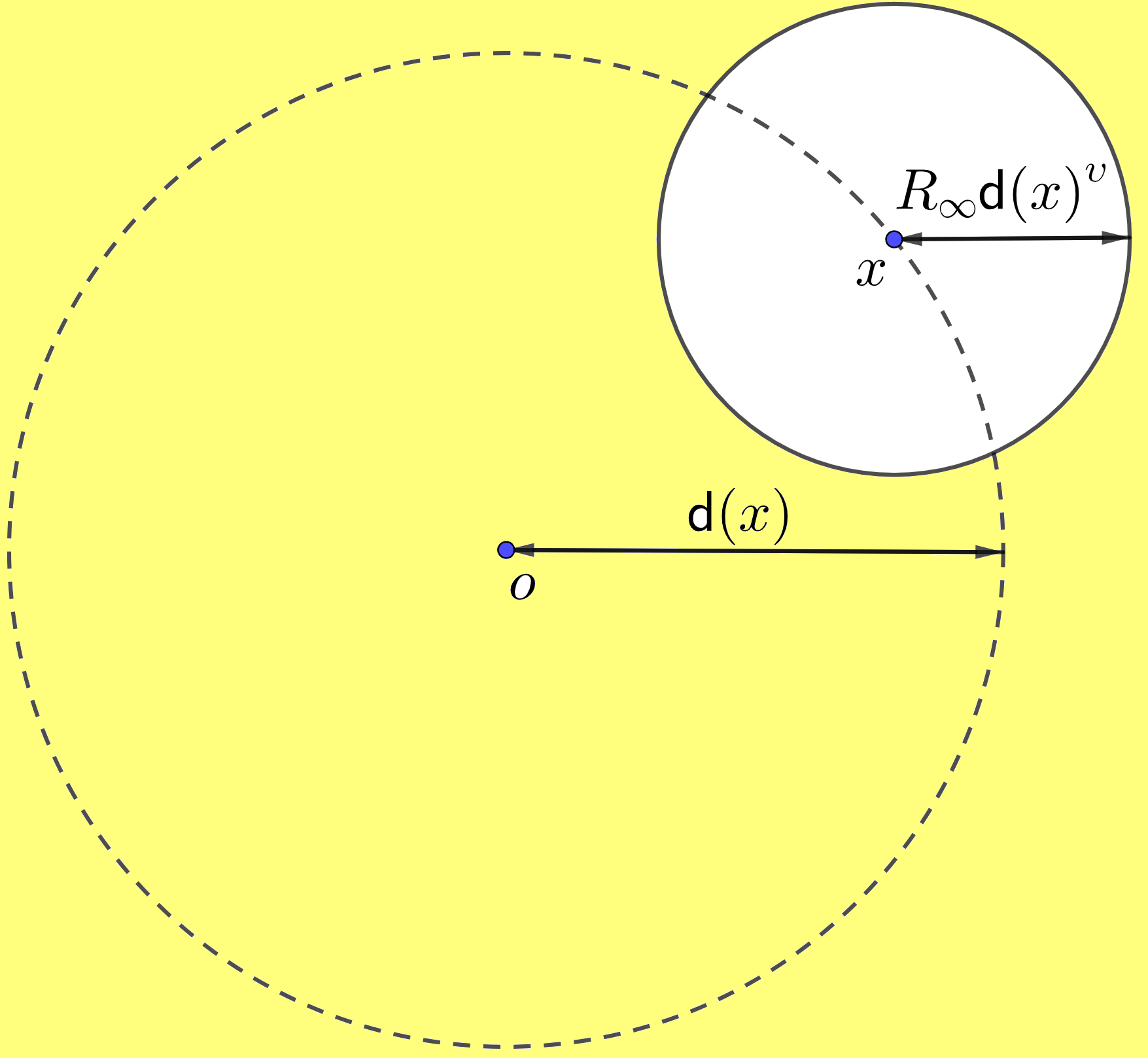
Figure 1. Range of $r$ in local conditions

Remark 1.1.

(i) Note that, like [12], we impose conditions at infinity (B1)-(B4) only for $r>R_{\infty}{\mathsf{d}}(x)^{\upsilon}$. By considering such weak assumptions at infinity, our LILs cover some random conductance models. See Section 3 below.

(ii) The assumptions (A3) and (B3) are quite mild and natural. Let $x\in U$. Suppose (A2) holds for $U$ and for $0<r<R_{0}\wedge(C_{0}\updelta_{U}(x))$

$$J(y,M_{\partial}\setminus B(x,r))\geq cJ(x,M_{\partial}\setminus B(x,r))\quad\text{ for all }y\in B(x,r/2).$$

Then, by the Lévy system, we have that for $0<r<R_{0}\wedge(C_{0}\updelta_{U}(x))$

$$1 \geq{\mathbb{P}}^{x}(X_{\tau_{B(x,r/2)}}\in M_{\partial}\setminus B(x,r))={\mathbb{E}}^{x}\left[\int_{0}^{\tau_{B(x,r/2)}}\int_{M_{\partial}\setminus B(x,r)}J(X_{s},dy)ds\right]$$

$$\geq c\,{\mathbb{E}}^{x}[\tau_{B(x,r/2)}]J(x,M_{\partial}\setminus B(x,r))\geq c\,C_{2}^{-1}{\mathbb{E}}^{x}[\tau_{B(x,r)}]J(x,M_{\partial}\setminus B(x,r)).$$

(iii) The lower inequality in (B2) implies that $\lim_{r\to\infty}{\mathbb{E}}^{o}[\tau_{B(o,r)}]=\infty$. Hence, under (B1) and (B2), we have $\lim_{r\to\infty}{\mathbb{E}}^{x}[\tau_{B(x,r)}]=\infty$ for all $x\in M$.

(iv) We need the lower inequality in (B2) because the space $M$ may be highly inhomogeneous. This inequality implies that the map $r\mapsto{\mathbb{E}}^{o}[\tau_{B(x,r)}]$ grows at least polynomially for large values of $r$. Hence under this condition, with a high probability, $X_{t}$ is not located in regions extremely far away from the base point $o$ in view of the time $t$ where we do not impose any conditions.

From now on, whenever condition (A1)-(A3) are assumed with $R_{0}>0$ for an open set $U$, we let $\phi(x,r)$ be any increasing function defined on $U\times(0,R_{0})$ which satisfies the following condition: There is a constant $C\geq 1$ such that for all $x\in U$ and $0<r<R_{0}\wedge(C_{0}\updelta_{U}(x))$,

$$C^{-1}{\mathbb{E}}^{x}[\tau_{B(x,r)}]\leq\phi(x,r)\leq C{\mathbb{E}}^{x}[\tau_{B(x,r)}].$$ (2)

Also, whenever condition (B1)-(B3) are assumed with $R_{\infty}\geq 1$ and ${\upsilon}\in(0,1)$, we let $\phi(r)$ be any function on $M\times(0,\infty)$ satisfying (2) for all $x\in M$ and $r>R_{\infty}{\mathsf{d}}(x)^{\upsilon}$, with $\phi(r)$ instead of $\phi(x,r)$.

Then by condition (A2), we see that there exist constants $\beta_{2}>0$ and $C_{U}\geq 1$ such that

$$\frac{\phi(x,r)}{\phi(x,s)}\leq C_{U}\bigg{(}\frac{r}{s}\bigg{)}^{\beta_{2}}\quad\text{for all}\;x\in U,\;0<s\leq r<R_{0}\wedge(C_{0}\updelta_{U}(x)),$$ (3)

and by (B2), there exist constants $\beta_{1},\beta_{2}>0$ and $C_{U}\geq 1\geq C_{L}>0$ such that

$$C_{L}\bigg{(}\frac{r}{s}\bigg{)}^{\beta_{1}}\leq\frac{\phi(r)}{\phi(s)}\leq C_{U}\bigg{(}\frac{r}{s}\bigg{)}^{\beta_{2}}\quad\text{for all}\;r\geq s>R_{\infty}{\mathsf{d}}(x)^{\upsilon}.$$ (4)

Now, we give our results in full generality. Our first result is the liminf law of LIL at zero. Note that we don’t put any extra assumptions on our metric measure space such as volume doubling property.

Theorem 1.2.

Suppose that (A1)-(A4) hold for an open subset $U\subset M$. Then, there are constants $a_{2}\geq a_{1}>0$ such that for all $x\in U$, there exists a constant $a_{x}\in[a_{1},a_{2}]$ satisfying

$$\liminf_{t\to 0}\frac{\phi\big{(}x,\sup_{0<s\leq t}d(x,X_{s})\big{)}}{t/\log|\log t|}=a_{x},\qquad{\mathbb{P}}^{x}\mbox{-a.s.}$$ (5)

Note that in Theorem 1.2, $r\mapsto\phi(x,r)$ for $x\in U$ can be slowly varying at zero so that we can cover jump processes whose jumping measures have logarithmic tails. When $\phi(x,r)$ is a mixed polynomial type near zero (i.e., both (3) and (6) hold), we recover the classical form of the liminf LIL at zero.

We denote $\phi^{-1}(x,t):=\sup\{r>0:\phi(x,r)\leq t\}$ for the right continuous inverse of $\phi(x,\cdot)$.

Corollary 1.3.

Suppose that (A1)-(A4) hold for an open subset $U\subset M$ and there exist constants $\beta_{1},C_{L}>0$ such that

$$\frac{\phi(x,r)}{\phi(x,s)}\geq C_{L}\bigg{(}\frac{r}{s}\bigg{)}^{\beta_{1}}\quad\text{for all}\;x\in U,\;0<s\leq r<R_{0}\wedge(C_{0}\updelta_{U}(x)).$$ (6)

Then, there are constants $\widetilde{a}_{2}\geq\widetilde{a}_{1}>0$ such that for all $x\in U$, there exists a constant $\widetilde{a}_{x}\in[\widetilde{a}_{1},\widetilde{a}_{2}]$ satisfying

$$\liminf_{t\to 0}\frac{\sup_{0<s\leq t}d(x,X_{s})}{\phi^{-1}(x,t/\log|\log t|)}=\widetilde{a}_{x},\qquad{\mathbb{P}}^{x}\mbox{-a.s.}$$ (7)

Our second result is the liminf law of LIL at infinity.

Theorem 1.4.

Suppose that (B1)-(B4) hold. Then, there are constants $b_{2}\geq b_{1}>0$ such that

$$\liminf_{t\to\infty}\frac{\sup_{0<s\leq t}d(x,X_{s})}{\phi^{-1}(t/\log\log t)}\in[b_{1},b_{2}],\qquad{\mathbb{P}}^{y}\mbox{-a.s.}\;\;\forall x,y\in M.$$ (8)

The $\liminf$ in (8) may not be deterministic. In [12], we have obtained a zero-one law for shift-invariant events under volume of doubling assumptions and near diagonal lower estimates on heat kernel (see Proposition 5.4 below). Using the same zero-one law, in this paper we also establish the deterministic limit in liminf law.

We recall following versions of volume doubling property from authors’ previous paper [12].

Definition 1.5.

(i) For an open set $U\subset M$ and $R_{0}^{\prime}\in(0,\infty]$, we say that the interior volume doubling and reverse doubling property ${\mathrm{VRD}}_{R_{0}^{\prime}}(U)$  holds if there exist constants $C_{V}\in(0,1)$, $d_{2}\geq d_{1}>0$ and $C_{\mu}\geq c_{\mu}>0$ such that for all $x\in U$ and $0<s\leq r<R_{0}^{\prime}\wedge(C_{V}\updelta_{U}(x))$,

$$c_{\mu}\left(\frac{r}{s}\right)^{d_{1}}\leq\frac{V(x,r)}{V(x,s)}\leq C_{\mu}\left(\frac{r}{s}\right)^{d_{2}}.$$ (9)

(ii) For $R_{\infty}^{\prime}\geq 1$ and ${\upsilon}\in(0,1)$, we say that a weak volume doubling and reverse doubling property at infinity ${\mathrm{VRD}}^{R_{\infty}^{\prime}}({\upsilon})$ holds if there exist constants $d_{2}\geq d_{1}>0$ and $C_{\mu}\geq c_{\mu}>0$ such that (9) holds for all $x\in M$ and $r\geq s>R_{\infty}^{\prime}{\mathsf{d}}(x)^{\upsilon}$.

For an open set $D\subset M$, let $X^{D}$ be the part process of $X$ defined as $X_{t}^{D}:=X_{t}\,{\bf 1}_{\{\tau_{D}>t\}}+\partial\,{\bf 1}_{\{\tau_{D}\leq t\}}$. Then $X_{t}$ is a Borel standard process on $D$. See, e.g. [8, Section 3.3]. Let $(P^{D}_{t})_{t\geq 0}$ be the semigroup associated with $X^{D}$, namely, $P^{D}_{t}f(x):={\mathbb{E}}^{x}[f(X^{D}_{t})]$. We call a Borel measurable function $p^{D}:(0,\infty)\times D\times D\to[0,\infty]$ the heat kernel (transition density) of $(P^{D}_{t})_{t\geq 0}$ (or $X^{D}$) if the followings hold:

(i) $P^{D}_{t}f(x)=\int_{D}p^{D}(t,x,y)f(y)\mu(dy)$ for all $t>0$, $x\in D$ and $f\in L^{\infty}(D;\mu)$.

(ii) $p^{D}(t+s,x,y)=\int_{D}p^{D}(t,x,z)p^{D}(s,z,y)\mu(dz)$ for all $t,s>0$ and $x,y\in D$.

We simply write $P_{t}$ for $P_{t}^{M}$ and $p(t,x,y)$ for $p^{M}(t,x,y)$.

We now consider the following near diagonal lower estimates on heat kernels:

There exist constants $$R_{\infty}^{\prime}\geq 1 {\upsilon},\eta\in(0,1) c_{*}>0 x\in M$$, , such that for all and

$$r>R_{\infty}^{\prime}{\mathsf{d}}(x)^{\upsilon} p^{B(x,r)}(t,x,y) X^{B(x,r)}$$, the heat kernel of exists and

$$p^{B(x,r)}(\phi(\eta r),y,z)\geq\frac{c_{*}}{V(x,r)}\quad\text{for all}\;\,y,z\in B(x,\eta^{2}r).$$ (B4+)

Under (B1) and ${\mathrm{VRD}}^{R_{\infty}^{\prime}}({\upsilon})$, the above condition (B4+) is stronger than (B4). See Proposition 1.9 below.

Remark 1.6.

The standard version of near diagonal lower estimates on heat kernels (without the restriction $r>R_{\infty}{\mathsf{d}}(x)^{\upsilon}$) has been studied a lot. In particular, in [10] and [11], it is shown that, for a large class of symmetric Hunt process, the standard version of near diagonal lower estimates on heat kernels can be obtained under (B2) and a Hölder-type regularity of corresponding harmonic functions See. [10, Proposition 4.9] and its proof.

Corollary 1.7.

Suppose that ${\mathrm{VRD}}^{R_{\infty}^{\prime}}({\upsilon})$ holds. If (B1), (B2), (B3) and (B4+) hold, then there exists a constant $b_{\infty}\in(0,\infty)$ such that

$$\liminf_{t\to\infty}\frac{\sup_{0<s\leq t}d(x,X_{s})}{\phi^{-1}(t/\log\log t)}=b_{\infty},\qquad{\mathbb{P}}^{y}\mbox{-a.s.}\;\;\forall x,y\in M.$$ (10)

Remark 1.8.

(i) Once we prove that the liminf LILs (5) and (7) hold true with $\phi(x,r)={\mathbb{E}}^{x}[\tau_{B(x,r)}]$, by the Blumenthal’s zero-one law, they hold true with general $\phi$ satisfying (2) after redefining constants $a_{1},a_{2},\widetilde{a}_{1},\widetilde{a}_{2}$ by $C^{-1}a_{1},Ca_{2},C^{-1}\widetilde{a}_{1},C\,\widetilde{a}_{2}$, respectively, with the constant $C\geq 1$ in (2). Similarly, thanks to the zero-one law given in Proposition 5.4, it suffices to prove Theorem 1.4 and Corollary 1.7 with a particular function $\phi(r):={\mathbb{E}}^{o}[\tau_{B(o,r)}]$.

(ii) Using the zero-one law in Proposition 5.4 again, we see that the liminf LIL (10) remains true even if the function $\phi$, which comes from condition (B4+), is replaced by any function $\widetilde{\phi}$ comparable to $\phi$.

Let us also consider the following counterpart of (B4+):

For a given open set $$U\subset M R_{0}^{\prime}>0 C_{0}^{\prime},\eta\in(0,1) c_{*}>0$$, there exist constants , and such that

for all $$x\in U 0<r<R_{0}^{\prime}\wedge(C_{0}^{\prime}\updelta_{U}(x)) p^{B(x,r)}(t,x,y) X^{B(x,r)}$$ and , the heat kernel of exists and

$$p^{B(x,r)}(\phi(x,\eta r),y,z)\geq\frac{c_{*}}{V(x,r)}\quad\text{for all}\;\,y,z\in B(x,\eta^{2}r).$$ (A4+)

Proposition 1.9.

(i) Suppose that ${\mathrm{VRD}}_{R_{0}^{\prime}}(U)$ holds. If (A2) and (A4+) hold, then (A4) holds with some $R_{0}>0$ and $C_{0}\in(0,1)$.

(ii) Suppose that ${\mathrm{VRD}}^{R_{\infty}^{\prime}}({\upsilon})$ holds. If (B2) and (B4+) hold, then (B4) holds with some $R_{\infty}\geq 1$.

Proof.

(i) By following the proof of [12, Proposition 4.3(i)] and using $\phi(x,r)$ instead of $\phi(r)$ therein, we can deduce that there exist constants $R_{1},c_{2},c_{3}>0$, $c_{1}>1$ and $C_{0}\in(0,1)$ such that for all $x\in U$, $0<c_{1}r<R_{1}\wedge(C_{0}\updelta_{U}(x))$ and $n\geq 1$,

$$e^{-c_{2}n}\leq{\mathbb{P}}^{x}\big{(}\tau_{B(x,r)}\geq n{\mathbb{E}}^{x}[\tau_{B(x,c_{1}r)}](x,c_{1}r)\big{)}\leq e^{-c_{3}n}.$$

By taking $R_{1}$ small enough if needed, we may assume that (A2) holds with $R_{0}=R_{1}$. Using (3), it follows that for all $x\in U$, $0<r<R_{1}\wedge(C_{0}\updelta_{U}(x))$ and $n\geq 1$,

$$e^{-c_{2}n} \leq{\mathbb{P}}^{x}\big{(}\tau_{B(x,r)}\geq n\phi(x,c_{1}r)\big{)}\leq{\mathbb{P}}^{x}\big{(}\tau_{B(x,r)}\geq n\phi(x,r)\big{)}$$

$$\leq{\mathbb{P}}^{x}\big{(}\tau_{B(x,r)}\geq c_{1}^{-\beta_{2}}C_{U}^{-1}n\phi(x,c_{1}r)\big{)}\leq e^{-c_{3}(c_{1}^{-\beta_{2}}C_{U}^{-1}n-1)}.$$

(ii) Analogously, we can deduce the result by following the proof of [12, Proposition 4.3(ii)]. ∎

The rest of the paper is organized as follows. In Sections 2–4, we show that the conditions (A1)-(A4), (B1)-(B4) and (B4+) can be checked for important classes of Markov jump processes, which may be non-symmetric and space-inhomogeneous. Thus we can apply our main theorems to get explicit liminf LILs for them.

Precisely, in Section 2, we consider general (non-symmetric) Feller processes on ${\mathbb{R}}^{d}$ whose domain of the generator contains $C_{c}^{\infty}({\mathbb{R}}^{d})$ and introduce some local assumptions (see (O1)-(O4) below). Under these assumptions, we establish liminf LIL at zero for Feller processes on ${\mathbb{R}}^{d}$. Then, combining results in this paper and [12], we present concrete examples of non-symmetric Feller processes and Feller processes with singular Lévy measures for which both liminf LILs and limsup LILs hold. In the remainder of Section 2, we give another assumption (see (S) below), which can be checked directly from the symbols of Feller processes. As a consequence, we show that liminf LILs at zero holds for Feller processes with symbols of varying order.

Section 3 revisits [12, Section 3] and discuss liminf LILs for the random conductance model with long range jumps studied in [6, 7]. Our conditions at infinity is motivated by the random conductance model therein.

In Section 4, we deal with subordinate processes and symmetric Hunt processes whose tail of the Lévy measure decays in (mixed) polynomial order. We assume that there is a Hunt process $Z$ enjoying sub-Gaussian heat kernel estimates. Then we show that general liminf LIL holds true for every subordinate process of $Z$ if the corresponding subordinator is not a compound Poisson process. In particular, we get liminf LILs for jump processes with low intensity of small jumps such as geometric stable processes. Using local stability theorems obtained in [12], we also get liminf LIL for symmetric Hunt processes associated with a regular Dirichlet form.

Section 5 is devoted to the proofs of our main theorems. We follow the well-known arguments in [16, Chapter 3], [27, Theorem 2] and [25, Theorem 3.7]. But non-trivial modifications are required since we allow our processes and state spaces to be highly space-inhomogeneous. The paper ends with Appendix 6 which contains some comparisons between conditions of the current paper and [12] and a simple lemma about lower heat kernel estimates for Dirichlet heat kernel.

Notations: Values of capital letters with subscripts $C_{i}$, $i=0,1,2,...$ are fixed throughout the paper both at zero and at infinity. Lower case letters with subscripts $a_{i}$, $c_{i}$, $i=0,1,2,...$ denote positive real constants and are fixed in each statement and proof, and the labeling of these constants starts anew in each proof. We use the symbol “$:=$” to denote a definition, which is read as “is defined to be.” Recall that $a\wedge b:=\min\{a,b\}$ and $a\vee b:=\max\{a,b\}$. We denote by $\overline{A}$ the closure of $A$. We extend a function $f$ defined on $M$ to $M_{\partial}$ by setting $f(\partial)=0$. The notation $f(x)\asymp g(x)$ means that there exist constants $c_{2}\geq c_{1}>0$ such that $c_{1}g(x)\leq f(x)\leq c_{2}g(x)$ for specified range of $x$. For $D\subset M$, denote by $C_{c}(D)$ the space of all continuous functions with compact support in $D$.

2. LIL for Feller processes on ${\mathbb{R}}^{d}$

Throughout this section, we assume that $X$ is a Feller process on ${\mathbb{R}}^{d}$ with the generator $({\cal L},{\cal D}({\cal L}))$ such that $C_{c}^{\infty}({\mathbb{R}}^{d})\subset{\cal D}({\cal L})$. It is well known that the generator ${\cal L}$ restricted to $C_{c}^{\infty}({\mathbb{R}}^{d})$ is a pseudo-differential operator, which has the following representation (see [15]):

$${\cal L}u(x)=-(2\pi)^{-d}\int_{{\mathbb{R}}^{d}}e^{i{\langle}x,\xi{\rangle}}q(x,\xi)\int_{{\mathbb{R}}^{d}}e^{-i{\langle}y,\xi{\rangle}}u(y)dyd\xi,\quad u\in C_{c}^{\infty}({\mathbb{R}}^{d}),$$

where the function $q:{\mathbb{R}}^{d}\times{\mathbb{R}}^{d}\to\mathbb{C}$, which is called the symbol of $X$ (or ${\cal L}$), enjoys the following Lévy-Khinchine formula

$$q(x,\xi)={\mathbf{c}}(x)-i{\langle}{\mathbf{b}}(x),\xi{\rangle}+{\langle}\xi,{\mathbf{a}}(x)\xi{\rangle}+\int_{{\mathbb{R}}^{d}\setminus\{0\}}(1-e^{i{\langle}z,\xi{\rangle}}+i{\langle}z,\xi{\rangle}{\bf 1}_{\{|z|\leq 1\}})\nu(x,dz).$$

Here $({\mathbf{c}}(x),{\mathbf{b}}(x),{\mathbf{a}}(x),\nu(x,dz))_{x\in{\mathbb{R}}^{d}}$ is a family of the Lévy characteristics, that is, ${\mathbf{c}}:{\mathbb{R}}^{d}\to[0,\infty)$ and ${\mathbf{b}}:{\mathbb{R}}^{d}\to{\mathbb{R}}^{d}$ are measurable functions, ${\mathbf{a}}:{\mathbb{R}}^{d}\to{\mathbb{R}}^{d\times d}$ is a nonnegative definite matrix-valued function, and $\nu(x,dz)$ is a nonnegative, $\sigma$-finite kernel on ${\mathbb{R}}^{d}\times{\cal B}({\mathbb{R}}^{d}\setminus\{0\})$ such that $\int_{{\mathbb{R}}^{d}\setminus\{0\}}(1\land|z|^{2})\nu(x,dz)<\infty$ for every $x\in{\mathbb{R}}^{d}$. Throughout this section, we always assume that ${\mathbf{c}}(x)$ is identically zero so that $X$ has no killing inside.

Define for $x\in{\mathbb{R}}^{d}$ and $r>0$,

$$\Phi(x,r)=\bigg{(}\sup_{|\xi|\leq 1/r}\text{Re}\,q(x,\xi)\bigg{)}^{-1}.$$ (11)

For example, if $q(x,\xi)=|\xi|^{\alpha(x)}(\log(1+|\xi|))^{\gamma(x)}$, then $\Phi(x,r)=r^{\alpha(x)}(\log(1+1/r))^{-\gamma(x)}$.

Here are our assumptions on the Feller process $X$. Let $U\subset{\mathbb{R}}^{d}$ be an open subset.

There exist constants $R_{0},\varepsilon_{0}>0$, $C_{i}\in(0,1)$, $8\leq i\leq 11$ such that for every $x\in U$ and $\xi\in{\mathbb{R}}^{d}$ with $1/|\xi|<R_{0}\wedge(C_{8}\updelta_{U}(x))$, the following hold

$$\lim_{r\to 0}\Phi(x,r)=0\quad\text{(or, equivalently, either ${\mathbf{a}}(x)\neq 0$ or $\nu(x,{\mathbb{R}}^{d})=\infty$)},$$ (O1)

$$\sup_{|\xi^{\prime}|\leq|\xi|}\text{Re}\,q(x,\xi^{\prime})\geq C_{9}|\,\text{Im}\,q(x,\xi)|,$$ (O2)

$$\inf_{|x-y|\leq 1/|\xi|}\textrm{Re}\,q(y,\xi)\geq C_{10}\sup_{|x-y|\leq 1/|\xi|}\textrm{Re}\,q(y,\xi),$$ (O3)

$${\mathbb{P}}^{x}\big{(}2{\langle}X_{t}-x,z{\rangle}\leq-|X_{t}-x|\big{)}\geq C_{11}\quad\text{for all}\;\;|z|=1\;\text{and}\;0<t<\varepsilon_{0}\Phi\big{(}x,R_{0}\wedge(C_{8}\updelta_{U}(x))\big{)}.$$ (O4)

Under (O1), the probability that the process $X$ starting from $x\in U$ stays at $x$ for a positive time is zero. (O2) is not only a local formulation of the sector condition but also a weaker version of it since we take the supremum in the left-hand side. (O3) and (O4) give a weak spatial homogeneity of the process in $U$. Similar conditions are appeared in [27] (see (A2)-(A3) therein) where small time Chung-type LILs for one-dimensional Lévy-type processes were studied.

Remark 2.1.

When $d=1$, (O4) is equivalent to ${\mathbb{P}}^{x}(X_{t}-x\geq 0)\in[C_{11},1-C_{11}]$ for all $x\in U$ and $t\leq\Phi\big{(}x,R_{0}\wedge(C_{8}\updelta_{U}(x))\big{)}$. Thus, if $d=1$ and $X$ is symmetric, then (O4) holds with $C_{11}=1/2$.

Following [30], we set for $x\in{\mathbb{R}}^{d}$ and $r>0$,

$$h(x,r)=\frac{1}{r^{2}}\lVert{\mathbf{a}}(x)\rVert+\int_{{\mathbb{R}}^{d}}\left(\frac{|z|^{2}}{r^{2}}\land 1\right)\nu(x,dz),$$ (12)

where $\lVert{\mathbf{a}}(x)\rVert:=\sup_{\xi\in{\mathbb{R}}^{d},\,|\xi|\leq 1}{\langle}\xi,{\mathbf{a}}(x)\xi{\rangle}$. The function $h$ frequently appears in maximal inequalities for Lévy-type processes. See, e.g. [16, 27].

The following result is well-known. We give a full proof for the reader’s convenience.

Lemma 2.2.

There exists a constant $C_{12}>1$ which depends only on the dimension $d$ such that

$$\sup_{|\xi|\leq 1/r}\text{\rm Re}\,q(x,\xi)\leq 2h(x,r)\leq C_{12}\sup_{1/(2r)\leq|\xi|\leq 1/r}\text{\rm Re}\,q(x,\xi)\quad\text{for all}\;\;x\in{\mathbb{R}}^{d},\;r>0.$$

In particular, it holds that

$$\frac{1}{2h(x,r)}\leq\Phi(x,r)\leq\frac{C_{12}}{2h(x,r)}\quad\text{for all}\;\;x\in{\mathbb{R}}^{d},\;r>0.$$ (13)

Proof.

Using the inequality $1-\cos y\leq y^{2}\wedge 2$ for $y\in{\mathbb{R}}$, we get that for all $x\in{\mathbb{R}}^{d}$ and $r>0$,

$$\sup_{|\xi|\leq 1/r}\text{Re}\,q(x,\xi)\leq\frac{1}{r^{2}}\lVert{\mathbf{a}}(x)\rVert+\sup_{|\xi|\leq 1/r}\int_{{\mathbb{R}}^{d}}(1-\cos{\langle}z,\xi{\rangle})\nu(x,dz)\leq 2h(x,r).$$

Next, it is clear that $\sup_{1/(2r)\leq|\xi|\leq 1/r}\text{Re}\,q(x,\xi)\geq r^{-2}\lVert{\mathbf{a}}(x)\rVert$. Moreover, using Tonelli’s theorem and the inequality $1-\cos y\geq y^{2}/4$ for $|y|\leq 1$, we get that for all $x\in{\mathbb{R}}^{d}$ and $r>0$,

$$\sup_{1/(2r)\leq|\xi|\leq 1/r}\text{Re}\,q(x,\xi)\geq c_{1}\int_{1/2\leq|\rho|\leq 1}\text{Re}\,q(x,\rho/r)d\rho$$

$$\geq c_{1}\int_{{\mathbb{R}}^{d}}\int_{1/2\leq|\rho|\leq 1}(1-\cos{\langle}z,\rho/r{\rangle})d\rho\,\nu(x,dz)$$

$$\geq c_{1}\left(\int_{|z|\leq r}\frac{|z|^{2}}{r^{2}}\int_{1/2\leq|\rho|\leq 1}\hskip-7.22743pt\frac{{\langle}z/|z|,\rho{\rangle}^{2}}{4}d\rho\nu(x,dz)+\int_{|z|>r}\int_{1/2\leq|\rho|\leq 1}\hskip-14.45377pt(1-\cos{\langle}z/r,\rho{\rangle})d\rho\,\nu(x,dz)\right)$$

$$\geq c_{1}\int_{{\mathbb{R}}^{d}}\left(\frac{|z|^{2}}{r^{2}}\land 1\right)\nu(x,dz)\inf_{y\in{\mathbb{R}}^{d},\,|y|=1}\left(\int_{1/2\leq|\rho|\leq 1}\hskip-7.22743pt\frac{{\langle}y,\rho{\rangle}^{2}}{4}d\rho\wedge\int_{1/2\leq|\rho|\leq 1}(1-\cos{\langle}y,\rho{\rangle})d\rho\right).$$

Let $\mathbf{e}_{1}:=(1,0,...,0)\in{\mathbb{R}}^{d}$. By the symmetry, we see that for all $y\in{\mathbb{R}}^{d}$ with $|y|=1$,

$$\int_{1/2\leq|\rho|\leq 1}{\langle}y,\rho{\rangle}^{2}d\rho\geq\int_{1/2\leq|\rho|\leq 1,\,{\langle}\mathbf{e}_{1},\rho{\rangle}\geq|\rho|/2}{\langle}\mathbf{e}_{1},\rho{\rangle}^{2}d\rho\geq\frac{1}{16}\int_{1/2\leq|\rho|\leq 1,\,{\langle}\mathbf{e}_{1},\rho{\rangle}\geq|\rho|/2}d\rho=c_{2}$$

and

$$\int_{1/2\leq|\rho|\leq 1}(1-\cos{\langle}y,\rho{\rangle})d\rho=\inf_{a>1}\int_{1/2\leq|\rho|\leq 1}(1-\cos a{\langle}\mathbf{e}_{1},\rho{\rangle})d\rho$$

$$\geq 2\inf_{a>1}\int_{0}^{1/2}\int_{\widetilde{\rho}\in{\mathbb{R}}^{d-1},|\widetilde{\rho}|\leq 1/2}(1-\cos a\rho_{1})d\widetilde{\rho}d\rho_{1}\geq c_{3}\inf_{a>1}\int_{0}^{1/2}(1-\cos a\rho_{1})d\rho_{1}.$$

Since $\lim_{a\to\infty}\int_{0}^{1/2}(1-\cos a\rho_{1})d\rho_{1}=1/2$, it holds that $\inf_{a>1}\int_{0}^{1/2}(1-\cos a\rho_{1})d\rho_{1}>0$. Therefore, using the inequality $a\vee b\geq(a+b)/2$ for $a,b\in{\mathbb{R}}$, we get that $\sup_{1/(2r)\leq|\xi|\leq 1/r}$ $\text{Re}\,q(x,\xi)$ $\geq$ $c_{4}h(x,r)$ and finish the proof. ∎

Recall that $\Phi$ is defined in (11). It is clear that $s^{2}h(x,s)\leq r^{2}h(x,r)$ for all $x\in{\mathbb{R}}^{d}$ and $0<s\leq r$. Thus, by (13), there exists a constant $C_{U}^{\prime}>0$ depends only on $d$ such that

$$\frac{\Phi(x,r)}{\Phi(x,s)}\leq C_{U}^{\prime}\bigg{(}\frac{r}{s}\bigg{)}^{2}\quad\text{for all}\;x\in{\mathbb{R}}^{d},\;0<s\leq r.$$ (14)

Lemma 2.3.

Suppose that (O3) holds for an open subset $U\subset{\mathbb{R}}^{d}$. Then there exists a constant $C_{13}\in(0,1)$ such that

$$\inf_{|x-y|\leq 2r}\Phi(y,r)\geq C_{13}\sup_{|x-y|\leq 2r}\Phi(y,r)\quad\text{for all}\;\;x\in U,\;0<4r<R_{0}\wedge(C_{8}\updelta_{U}(x)).$$

Proof.

By (14), Lemma 2.2 and (O3), we get that for all $x\in U$ and $0<4r<R_{0}\wedge(C_{8}\updelta_{U}(x))$,

$$\inf_{|x-y|\leq 2r}\Phi(y,r)\geq c_{1}\inf_{|x-y|\leq 2r}\bigg{(}\sup_{1/(4r)\leq|\xi|\leq 1/(2r)}\text{Re}\,q(y,\xi)\bigg{)}^{-1}$$

$$=c_{1}\inf_{1/(4r)\leq|\xi|\leq 1/(2r)}\,\inf_{|x-y|\leq 2r}\text{Re}\,q(y,\xi)^{-1}\geq c_{1}C_{10}\inf_{1/(4r)\leq|\xi|\leq 1/(2r)}\,\sup_{|x-y|\leq 2r}\text{Re}\,q(y,\xi)^{-1}$$

$$\geq c_{2}\sup_{|x-y|\leq 2r}\,\inf_{1/(4r)\leq|\xi|\leq 1/(2r)}\text{Re}\,q(y,\xi)^{-1}\geq c_{2}C_{10}\sup_{|x-y|\leq 2r}\Phi(x,r).$$

∎

As an application of our Theorem 1.2, we obtain the following LIL for Feller processes. See [27, Theorem 2] for a 1-dimensional result under similar assumptions.

Theorem 2.4.

Let $X$ be a Feller process on ${\mathbb{R}}^{d}$ with symbol $q$. Suppose that (O1)-(O4) hold for an open subset $U\subset{\mathbb{R}}^{d}$. Then, there are constants $a_{2}\geq a_{1}>0$ such that for all $x\in U$, there exists a constant $a_{x}\in[a_{1},a_{2}]$ satisfying

$$\liminf_{t\to 0}\frac{\Phi(x,\,\sup_{0<s\leq t}|X_{s}-x|)}{t/\log|\log t|}=a_{x},\qquad{\mathbb{P}}^{x}\mbox{-a.s.}$$ (15)

Moreover, if there exist constants $\beta_{1}^{\prime},C_{L}^{\prime}>0$ such that

$$\frac{\Phi(x,r)}{\Phi(x,s)}\geq C_{L}^{\prime}\bigg{(}\frac{r}{s}\bigg{)}^{\beta_{1}^{\prime}}\quad\text{for all}\;x\in U,\;0<s\leq r<R_{0}\wedge(C_{8}\updelta_{U}(x)),$$ (16)

then there are constants $\widetilde{a}_{2}\geq\widetilde{a}_{1}>0$ such that for all $x\in U$, there exists a constant $\widetilde{a}_{x}\in[\widetilde{a}_{1},\widetilde{a}_{2}]$ satisfying

$$\liminf_{t\to 0}\frac{\sup_{0<s\leq t}d(x,X_{s})}{\Phi^{-1}(x,t/\log|\log t|)}=\widetilde{a}_{x},\qquad{\mathbb{P}}^{x}\mbox{-a.s.}$$ (17)

Remark 2.5.

Let $\widetilde{\Phi}$ be any function on $U\times(0,1)$ such that $\widetilde{\Phi}(x,r)\asymp\Phi(x,r)$ for $x\in U$ and $r\in(0,1)$. Thanks to the Blumenthal’s zero-one law, the liminf LILs (15) and (17) hold true with $\widetilde{\Phi}$ instead of $\Phi$. Cf. Remark 1.8.

To prove Theorem 2.4, we need the following two lemmas.

The first one is a consequence of [4, Section 5]. Since we only put assumptions on the symbol $q$ locally, we carefully check ranges of variables in the proof of the following lemma.

Lemma 2.6.

Suppose that (O1), (O2) and (O3) hold for an open subset $U\subset{\mathbb{R}}^{d}$. Then there exist constants $C_{14},C_{15}>0$ and $C_{16}>1$ such that for all $x\in U$, $0<\frac{8C_{12}}{C_{9}}r<R_{0}\wedge(C_{8}\updelta_{U}(x))$, $w\in B(x,r)$ and $t>0$,

$${\mathbb{P}}^{w}(\tau_{B(w,r)}\leq t)\leq\frac{C_{14}t}{\Phi(x,r)},$$ (18)

$${\mathbb{P}}^{w}(\tau_{B(w,r)}\geq t)\leq\exp\bigg{(}-\frac{C_{15}t}{\Phi(x,r)}+1\bigg{)},$$ (19)

and

$$C_{16}^{-1}\Phi(x,r)\leq{\mathbb{E}}^{w}[\tau_{B(w,r)}]\leq C_{16}\Phi(x,r),$$ (20)

where $C_{9},C_{10}$ and $C_{12}$ are constants in (O2), (O3) and Lemma 2.2 respectively.

Proof.

Fix $x\in U$. Let $r_{0}:=R_{0}\wedge(C_{8}\updelta_{U}(x))$ and $k:=2C_{12}/C_{9}>2$. Note that for all $0<4kr<r_{0}$ and $w\in B(x,2r)$, by the triangle inequality,

$$C_{8}\updelta_{U}(w)\geq C_{8}(\updelta_{U}(x)-r)>r_{0}-2r>3kr.$$

Hence, by Lemma 2.2 and (O2), it holds that for all $0<4kr<r_{0}$ and $w\in B(x,r)$,

$$\sup_{1/(4kr)\leq|\xi|\leq 1/(2kr)}\sup_{|y-w|\leq r}\frac{\text{Re}\,q(y,\xi)}{|\xi||\text{Im}\,q(y,\xi)|}\geq\frac{2kr}{C_{12}}\frac{\sup_{|\xi|\leq 1/(kr)}\text{Re}\,q(w,\xi)}{\sup_{|\xi|\leq 1/(kr)}|\text{Im}\,q(w,\xi)|}\geq\frac{2C_{9}kr}{C_{12}}=4r.$$ (21)

Using (O3), Lemma 2.2 and the monotone property of $\Phi$, we get that for all $0<4kr<r_{0}$ and $w\in B(x,r)$,

$$\sup_{1/(4kr)\leq|\xi|\leq 1/(2kr)}\,\inf_{|y-w|\leq 3r}\text{Re}\,q(y,\xi)$$

$$\geq\sup_{1/(4kr)\leq|\xi|\leq 1/(2kr)}\,\inf_{|y-x|<4r}\text{Re}\,q(y,\xi)\geq C_{10}\sup_{1/(4kr)\leq|\xi|\leq 1/(2kr)}\text{Re}\,q(x,\xi)\geq\frac{C_{10}}{C_{12}}\Phi(x,r).$$ (22)

On the other hand, by Lemma 2.2 and (O3), we also get that for all $0<4r<r_{0}$ and $w\in B(x,r)$,

$$\sup_{|y-w|\leq r}\,\sup_{|\xi|\leq 1/r}\text{Re}\,q(y,\xi)\leq C_{12}\sup_{1/(2r)\leq|\xi|\leq 1/r}\,\sup_{|y-w|\leq r}\text{Re}\,q(y,\xi)\leq\frac{C_{12}}{C_{10}}\Phi(x,r)^{-1}.$$ (23)

Moreover, we get from Lemma 2.3 and (O2) that for all $0<4kr<r_{0}$ and $w\in B(x,r)$,

$$\sup_{|y-w|\leq r}\,\sup_{4/r_{0}<|\xi|\leq 1/r}|\text{Im}\,q(y,\xi)|\leq\frac{1}{C_{9}}\sup_{|y-x|<2r}\,\sup_{|\xi|\leq 1/r}|\text{Re}\,q(y,\xi)|\leq\frac{C_{13}}{C_{9}}\Phi(x,r)^{-1}.$$

Using the triangle inequality several times, (O2) in the second inequality, the inequality $|a-\sin a|\leq|a|^{2}$ for $a\in{\mathbb{R}}$ in the third, Lemma 2.2 in the fourth, and the monotone property of $\Phi$ and Lemma 2.3 in the last, we get that for all $y,\xi\in{\mathbb{R}}^{d}$ such that $|y-x|<2r$ and $|\xi|\leq 4/r_{0}$,

$$|\,\text{Im}\,q(y,\xi)| \leq\frac{r_{0}|\xi|}{4}\big{|}\,\text{Im}\,q(y,\frac{4}{r_{0}|\xi|}\xi)\big{|}+\bigg{|}\int_{{\mathbb{R}}^{d}}\bigg{(}\frac{r_{0}|\xi|}{4}\sin{\langle}z,\frac{4}{r_{0}|\xi|}\xi{\rangle}-\sin{\langle}z,\xi{\rangle}\bigg{)}\nu(y,dz)\bigg{|}$$

$$\leq\frac{r_{0}|\xi|}{4C_{9}}\Phi(y,4/r_{0})^{-1}+\frac{r_{0}|\xi|}{4}\int_{|z|<r_{0}/4}\bigg{|}{\langle}z,\frac{4}{r_{0}|\xi|}\xi{\rangle}-\sin{\langle}z,\frac{4}{r_{0}|\xi|}\xi{\rangle}\bigg{|}\,\nu(y,dz)$$

$$\quad+\int_{|z|<r_{0}/4}\big{|}{\langle}z,\xi{\rangle}-\sin{\langle}z,\xi{\rangle}\big{|}\nu(y,dz)+\bigg{(}\frac{r_{0}|\xi|}{4}+1\bigg{)}\int_{|z|\geq r_{0}/4}\nu(y,dz)$$

$$\leq\frac{1}{C_{9}}\Phi(y,4/r_{0})^{-1}+\bigg{(}\frac{16}{r_{0}^{2}}+\frac{16}{r_{0}^{2}}\bigg{)}\int_{|z|<r_{0}/4}|z|^{2}\nu(y,dz)+2\nu\big{(}y,{\mathbb{R}}^{d}\setminus B(0,r_{0}/4)\big{)}$$

$$\leq c_{1}\Phi(y,4/r_{0})^{-1}\leq c_{2}\Phi(x,r)^{-1}.$$

Therefore, we deduce that for all $0<4kr<r_{0}$ and $w\in B(x,r)$,

$$\sup_{|y-w|\leq r}\sup_{|\xi|\leq 1/r}|q(y,\xi)|\leq\sup_{|y-w|\leq r}\Big{(}\sup_{|\xi|\leq 1/r}\text{Re} q(y,\xi)+\sup_{4/r_{0}<|\xi|\leq 1/r}|\text{Im}\,q(y,\xi)|$$

$$+\sup_{|\xi|\leq 4/r_{0}}|\text{Im}\,q(y,\xi)|\Big{)}\leq c_{3}\Phi(x,r)^{-1}.$$ (24)

Finally, by (21), (2) and (2), we obtain the results from [4, Theorem 5.1, Corollary 5.3 and Theorem 5.9]. ∎

Lemma 2.7.

Suppose that (O1)-(O4) hold for an open subset $U\subset{\mathbb{R}}^{d}$. Then (A4) holds for $U$.

Proof.

By following the proof of [19, Proposition 5.2], one can deduce (A4) from (18), (19) and (O4). Below, we give the proof of this conclusion in details for the reader’s convenience.

Choose any $x\in U$ and set $r_{0}:=R_{0}\wedge(C_{8}\delta_{U}(x))$. For all $w\in B(x,r_{0}/8)$, since $\updelta_{U}(w)\geq\updelta_{U}(x)-r_{0}/8>\updelta_{U}(x)/5$, we get from Lemma 2.3 and (14) that

$$\Phi\big{(}w,R_{0}\wedge(C_{8}\updelta_{U}(w))\big{)}\geq\Phi(w,r_{0}/5)\geq C_{13}\Phi(x,r_{0}/5)\geq c_{1}\Phi(x,r_{0}),$$ (25)

where the constant $c_{1}>0$ is independent of $x$.

Let $0<\frac{8C_{12}}{C_{9}}r<r_{0}$. By (18) and (20), there is a constant $\varepsilon_{1}\in(0,c_{1}\varepsilon_{0}/C_{16})$ independent of $x$ and $r$ such that for all $w\in B(x,r/2)$,

$${\mathbb{P}}^{w}(\tau_{B(w,r/2)}\leq\varepsilon_{1}{\mathbb{E}}^{x}[\tau_{B(x,r)}])\leq\frac{C_{11}}{2},$$ (26)

where $\varepsilon_{0}$, $C_{11}$ and $C_{16}$ are the constants in (O4) and (20). We set $t_{0}:=\varepsilon_{1}{\mathbb{E}}^{x}[\tau_{B(x,r)}]$ and for $k\geq 0$,

$$S_{k}:=\left\{\sup_{kt_{0}\leq u\leq(k+1)t_{0}}|X_{u}-X_{kt_{0}}|<\frac{r}{2},\,2{\langle}X_{(k+1)t_{0}}-X_{kt_{0}},X_{kt_{0}}{\rangle}\leq-|X_{(k+1)t_{0}}-X_{kt_{0}}||X_{kt_{0}}|\right\}.$$

Note that, for any $y,z\in{\mathbb{R}}^{d}$, if $|y|,|z|<r/2$ and $2{\langle}y,z{\rangle}\leq-|y||z|$, then $|y+z|<r/2$. Thus, by the Markov property, we see that for all $n\geq 1$,

$${\mathbb{P}}^{x}(\tau_{B(x,r)}\geq nt_{0}) \geq{\mathbb{P}}^{x}\Big{(}\cap_{k=0}^{n-1}S_{k}\Big{)}={\mathbb{P}}^{x}{\mathbb{E}}\Big{[}\cap_{k=0}^{n-1}S_{k}\,\big{|}\,{\mathcal{F}}_{(n-1)t_{0}}\Big{]}$$

$$\geq\inf_{w\in B(x,r/2)}{\mathbb{P}}^{w}(S_{0})\cdot{\mathbb{P}}^{x}\Big{(}\cap_{k=0}^{n-2}S_{k}\Big{)}\geq...\geq\Big{(}\inf_{w\in B(x,r/2)}{\mathbb{P}}^{w}(S_{0})\Big{)}^{n}.\qquad$$ (27)

For all $w\in B(x,r/2)$, since $\varepsilon_{0}\Phi\big{(}w,R_{0}\wedge(C_{8}\updelta_{U}(w))\big{)}>c_{1}\varepsilon_{0}C_{16}^{-1}{\mathbb{E}}^{x}[\tau_{B(x,r)}]>t_{0}$ by (25) and (20), using (O4) and (26), we get that

$${\mathbb{P}}^{w}(S_{0}) \geq 1-{\mathbb{P}}^{w}(2{\langle}X_{t_{0}}-w,w{\rangle}>-|X_{t_{0}}-w||w|)-{\mathbb{P}}^{w}(\tau_{B(w,r/2)}\leq t_{0})\geq\frac{C_{11}}{2}.$$

It follows that for all $n\geq 1$,

$${\mathbb{P}}^{x}(\tau_{B(x,r)}\geq n{\mathbb{E}}^{x}[\tau_{B(x,r)}])={\mathbb{P}}^{x}(\tau_{B(x,r)}\geq n\varepsilon_{1}^{-1}t_{0})\geq\bigg{(}\frac{C_{11}}{2}\bigg{)}^{-\varepsilon_{1}^{-1}n+1}.$$

On the other hand, by (19) and (20), we get that for all $n\geq 1$,

$${\mathbb{P}}^{x}(\tau_{B(x,r)}\geq n{\mathbb{E}}^{x}[\tau_{B(x,r)}])\leq e^{-\frac{C_{15}}{C_{16}}n+1}.$$

The proof is complete. ∎

Proof of Theorem 2.4. With a redefined $R_{0}$, in view of (20), we get (A1) from Lemma 2.3, (A2) from (O1) and (14), (A3) from Lemma 2.2, and (A4) from Lemma 2.7. Then by the proof of Theorem 1.2, one can see that (72) below holds for all $x\in U$ with $\Phi(x,\cdot)$ instead of $\phi(x,\cdot)$. Hence, by the Blumenthal’s zero-one law, we deduce (15). Moreover, if (16) also holds true, then we arrive at (17) by a similar argument to that in the proof of Corollary 1.3. We omit details here. ∎

We now give concrete examples of Feller processes which satisfy both liminf LIL at zero and limsup LIL at zero with help from the paper [12]. In the following two examples, we use conditions Tail, E and NDL introduced in [12]. See Definitions 6.1–6.2 in Appendix for their definitions.

Example 2.8.

(Non-symmetric Feller processes) Let $\nu$ be a nonincreasing nonnegative function on $(0,\infty)$ satisfying $\int_{0}^{\infty}(r^{d-1}\land r^{d+1})\nu(r)dr<\infty$. Define for $r>0$,

$$\mathcal{G}(r)=1\bigg{/}\int_{|z|\geq r}\nu(|z|)dz\quad\text{and}\quad\mathcal{H}(r)=1\bigg{/}\int_{{\mathbb{R}}^{d}}\left(\frac{|z|^{2}}{r^{2}}\land 1\right)\nu(|z|)dz.$$

Then $\mathcal{H}\leq\mathcal{G}$, $\mathcal{H}$ is increasing and ${\cal H}(r)/{\cal H}(s)\leq(r/s)^{2}$ for all $0<s\leq r$. We assume that there exist constants $0<\beta_{1}\leq\beta_{2}\leq 2$ and $c_{1},c_{2}>0$ such that

$$c_{1}\bigg{(}\frac{r}{s}\bigg{)}^{\beta_{1}}\leq\frac{{\cal H}(r)}{{\cal H}(s)}\leq c_{2}\bigg{(}\frac{r}{s}\bigg{)}^{\beta_{2}}\quad\text{for all}\;\,0<s\leq r\leq 1.$$ (28)

Let $J(z)$ be a nonnegative function on ${\mathbb{R}}^{d}$ comparable to $\nu(|z|)$ and $\kappa(x,z)$ be a Borel function on ${\mathbb{R}}^{d}\times{\mathbb{R}}^{d}$ such that for some constants $a_{1},a_{2},a_{3}>0$ and $\beta\in(0,1)$,

$$a_{1}\leq\kappa(x,z)\leq a_{2}\quad\text{and}\quad|\kappa(x,z)-\kappa(y,z)|\leq a_{3}|x-y|^{\beta}\quad\text{for all}\;\,x,y,z\in{\mathbb{R}}^{d}.$$ (29)

In this example, we always suppose that one of the following assumptions holds true:

(P1) (28) holds with $\beta_{1}>1$,

(P2) (28) holds with $\beta_{2}<1$,

(P3) $J(z)=J(-z)$ and $\kappa(x,z)=\kappa(x,-z)$ for all $x,z\in{\mathbb{R}}^{d}$.

In each case when (P1), (P2) and (P3) holds, respectively, we consider an operator

$${\cal L}^{\kappa}f(x):=\begin{cases}\int_{{\mathbb{R}}^{d}}\big{(}f(x+z)-f(x)-{\bf 1}_{|z|\leq 1}\langle z,\nabla f(x)\rangle\big{)}\kappa(x,z)J(|z|)dz,&\text{if (P1) holds};\\ \int_{{\mathbb{R}}^{d}}\big{(}f(x+z)-f(x)\big{)}\kappa(x,z)J(|z|)dz,&\text{if (P2) holds};\\ \frac{1}{2}\int_{{\mathbb{R}}^{d}}\big{(}f(x+z)+f(x-z)-2f(x)\big{)}\kappa(x,z)J(|z|)dz&\text{if (P3) holds}.\end{cases}$$

According to [20, Theorem 1.3 and Remark 1.5], if (29) and one among (P1)-(P3) hold, then there exists a Feller process $X$ on ${\mathbb{R}}^{d}$ whose infinitesimal generator is an extension of $({\cal L}^{\kappa},C_{c}^{2}({\mathbb{R}}^{d}))$. Indeed, the process $X$ is the unique solution to the martingale problem for $({\cal L}^{\kappa},C_{c}^{\infty}({\mathbb{R}}^{d}))$. By Lemma 2.2 and (29), since $J(z)$ is comparable to $\nu(|z|)$, the symbol $q$ of $X$ satisfies that

$$\sup_{|\xi|\leq 1/r}\text{\rm Re}\,q(x,\xi)\asymp 1/{\cal H}(r)\quad\text{for}\;\,x\in{\mathbb{R}}^{d},\;r>0$$ (30)

In the followings, we check that $X$ satisfies conditions (O1)-(O4) for $U={\mathbb{R}}^{d}$.

First, we note that, by (28) and (29), $\int_{{\mathbb{R}}^{d}}\kappa(x,z)J(z)dz\geq c\int_{{\mathbb{R}}^{d}}\nu(|z|)dz=$ $c\lim_{r\to 0}1/{\cal H}(r)$ $=\infty$ for all $x\in{\mathbb{R}}^{d}$. Hence, (O1) holds for $U={\mathbb{R}}^{d}$.

When (P3) holds, the symbol $q(x,\xi)$ is a real number for all $x,\xi$ so that (O2) for $U={\mathbb{R}}^{d}$ immediately follows. We now check (O2) for the cases (P2) and (P3) separately.

Suppose (P1) holds. Using the triangle inequality, Taylor expansion for the sine function and (28), since $\kappa$ is bounded above, $J(z)$ is comparable to $\nu(|z|)$. Since $\nu(|z|)dz$ is a Lévy measure on ${\mathbb{R}}^{d}$ and $\beta_{1}>1$, we get that for all $x\in{\mathbb{R}}^{d}$ and $\xi\in{\mathbb{R}}^{d}$ with $|\xi|\geq 1$,

$$|\text{Im}\,q(x,\xi)| =\bigg{|}\int_{{\mathbb{R}}^{d}\setminus\{0\}}\big{(}\langle z,\xi\rangle{\bf 1}_{\{|z|\leq 1\}}-\sin\langle z,\xi\rangle\big{)}\kappa(x,z)J(z)dz\bigg{|}$$

$$\leq\bigg{|}\int_{|z|\leq 1}\big{(}\langle z,\xi\rangle-\sin\langle z,\xi\rangle\big{)}\kappa(x,z)J(z)dz\bigg{|}+\bigg{|}\int_{|z|>1}\sin\langle z,\xi\rangle\kappa(x,z)J(z)dz\bigg{|}$$

$$\leq c_{2}\int_{|z|\leq 1}\big{(}(|z||\xi|)^{3}\wedge(|z||\xi|)\big{)}\nu(|z|)dz+c_{2}\int_{|z|>1}\nu(|z|)dz$$

$$\leq c_{2}\int_{|z|\leq 1/|\xi|}(|z||\xi|)^{2}\nu(|z|)dz+c_{2}|\xi|\int_{1/|\xi|<|z|\leq 1}|z|^{2}\nu(|z|)dz+c_{3}$$

$$\leq\frac{c_{4}}{{\cal H}(1/|\xi|)}+\frac{c_{4}|\xi|+c_{3}{\cal H}(1)}{{\cal H}(1)}\leq\frac{c_{4}}{{\cal H}(1/|\xi|)}+\frac{(c_{4}+c_{3}{\cal H}(1))|\xi|}{c_{1}|\xi|^{\beta_{1}}{\cal H}(1/|\xi|)}\leq\frac{c_{5}}{{\cal H}(1/|\xi|)}.$$

Suppose (P2) holds. Using (28), since $\kappa$ is bounded above, $J(z)$ is comparable to $\nu(|z|)$. Using this fact and $\beta_{2}<1$, we see that for all $x\in{\mathbb{R}}^{d}$ and $\xi\in{\mathbb{R}}^{d}$ with $|\xi|\geq 1$,

$$|\text{Im}\,q(x,\xi)|=\bigg{|}\int_{{\mathbb{R}}^{d}\setminus\{0\}}\sin\langle z,\xi\rangle\kappa(x,z)J(z)dz\bigg{|}$$

$$\leq c_{6}|\xi|\int_{|z|<1/|\xi|}|z|\nu(|z|)dz+c_{6}\int_{|z|\geq 1/|\xi|}\nu(|z|)dz$$

$$\leq c_{6}\sum_{n\geq 1}\int_{2^{-n}/|\xi|\leq|z|<2^{-n+1}/|\xi|}2^{-n+1}\nu(|z|)dz+\frac{c_{6}}{{\cal H}(1/|\xi|)}$$

$$\leq c_{6}\sum_{n\geq 1}\frac{2^{-n+1}}{{\cal H}(2^{-n}/|\xi|)}+\frac{c_{6}}{{\cal H}(1/|\xi|)}\leq\frac{c_{2}c_{6}}{{\cal H}(1/|\xi|)}\sum_{n\geq 1}2^{-n+1+n\beta_{2}}+\frac{c_{6}}{{\cal H}(1/|\xi|)}=\frac{c_{7}}{{\cal H}(1/|\xi|)}.$$

Therefore, by (30), we deduce that (O2) always holds true for $U={\mathbb{R}}^{d}$.

(O3) immediately follows from the fact that $\kappa(x,z)$ is bounded above and below by positive constants. For (O4), we see from [20, (84)] that the heat kernel $p(t,x,y)$ of $X$ satisfies that for all $t\leq 1$ and $x,y\in{\mathbb{R}}^{d}$ with $|x-y|\leq{\cal H}^{-1}(t)$,

$$p(t,x,y)\geq c_{8}{\cal H}^{-1}(t)^{-d}.$$

It follows that for all $t\leq 1$, $x\in{\mathbb{R}}^{d}$ and $z\in{\mathbb{R}}^{d}$ with $|z|=1$,

$${\mathbb{P}}^{x}\big{(}2{\langle}X_{t}-x,z{\rangle}\leq-|X_{t}-x|\big{)}\geq\int_{B(x,{\cal H}^{-1}(t))\cap\{y:2{\langle}y-x,z{\rangle}\leq-|y-x|\}}p(t,x,y)dy$$

$$\geq c_{8}{\cal H}^{-1}(t)^{-d}\int_{B(x,{\cal H}^{-1}(t))\cap\{y:2{\langle}y-x,z{\rangle}\leq-|y-x|\}}dy=c_{8}\int_{B(0,1)\cap\{y:2{\langle}y,z{\rangle}\leq-|y|\}}dy=c_{9}.$$

Therefore, (O4) holds true for $U={\mathbb{R}}^{d}$.

Now, using (28) and (30), we conclude from Theorem 2.4 and Remark 2.5 that the liminf LIL at zero (17) holds true with $U={\mathbb{R}}^{d}$ and $\Phi^{-1}(x,t/\log|\log t|)$ replaced by ${\cal H}^{-1}(t/\log|\log t|)$.

To obtain a limsup LIL at zero for the Feller process $X$, we also assume that ${\mathrm{U}}_{r_{1}}(\mathcal{G},\gamma,c)$ (in Definition 6.3) holds for some $\gamma>0$ and $r_{1},c\in(0,1)$. Here, we emphasize that $\gamma$ may not be smaller than $2$. By (29), $\mathrm{Tail}_{\infty}(\mathcal{G},{\mathbb{R}}^{d})$ and $\mathrm{Tail}_{\infty}({\cal H},{\mathbb{R}}^{d},\leq)$ (in Definition 6.2(i)) hold. Moreover, by [20, Theorem 1.2(4) and Lemma 4.11] and our Lemma 6.5, $\mathrm{NDL}_{R_{0}^{\prime}}({\cal H},{\mathbb{R}}^{d})$ (in Definition 6.2(iii)) holds for some $R_{0}^{\prime}>0$. Therefore, using (28), we deduce that for all $x\in{\mathbb{R}}^{d}$, the limsup LIL at zero given in [12, Theorem 1.11(i-ii)] holds true for $X$ with functions $\phi={\cal H}$ and $\psi=\mathcal{G}$. ∎

In the following example, we directly check that conditions (A1)-(A4), (B1)-(B3) and (B4+) hold.

Example 2.9.

(Singular Lévy measure) Let $\alpha\in(0,2)$, $d\geq 2$ and ${\mathbb{R}}_{i}:=\{(x_{1},\dots,x_{d})\in{\mathbb{R}}^{d}:x_{j}=0\mbox{ if }j\neq i\}$ for $1\leq i\leq d$. Denote by $e^{i}$, $1\leq i\leq d$ the standard unit vectors in ${\mathbb{R}}^{d}$. Define a kernel $J(x,y)$ on ${\mathbb{R}}^{d}\times{\mathbb{R}}^{d}$ by

$$J(x,y)=\begin{cases}b(x,y)|x-y|^{-1-\alpha},\;\;&\mbox{if}\;\;y-x\in\cup_{i=1}^{d}{\mathbb{R}}_{i}\setminus\{0\},\\ 0,\;\;&\mbox{otherwise},\end{cases}$$ (31)

where $b(x,y)$ is a symmetric function on ${\mathbb{R}}^{d}\times{\mathbb{R}}^{d}$ that is bounded between two positive constants. Using this kernel, define a symmetric form $({\mathcal{E}},{\mathcal{F}})$ on $L^{2}({\mathbb{R}}^{d};dx)$ as

$$\begin{split}{\mathcal{E}}(u,v)&=\int_{{\mathbb{R}}^{d}}\Big{(}\sum_{i=1}^{d}\int_{{\mathbb{R}}}(u(x+e^{i}\tau)-u(x))(v(x+e^{i}\tau)-v(x))J(x,x+e^{i}\tau)d\tau\Big{)}dx,\\ {\mathcal{F}}&=\{u\in L^{2}({\mathbb{R}}^{d};dx)\,|\,{\mathcal{E}}(u,u)<\infty\}.\end{split}$$

According to [36, Theorem 3.9 and Corollary 4.15], the above form $({\mathcal{E}},{\mathcal{F}})$ is a regular Dirichlet form and the associated Hunt process $X$ is a strong Feller process in ${\mathbb{R}}^{d}$. Below, we get liminf and limsup LILs for $X$, both at zero and at infinity.

From the definition (31), we see that $\mathrm{Tail}_{\infty}(r^{\alpha},{\mathbb{R}}^{d})$ holds true. Indeed, for all $x\in{\mathbb{R}}^{d}$ and $r>0$, $\int_{B(x,r)^{c}}J(x,dy)=\sum_{i=1}^{d}\int_{|\tau|\geq r}J(x,x+\tau e^{i})d\tau\asymp d\int_{|\tau|\geq r}\tau^{-1-\alpha}d\tau=cr^{-\alpha}$. By [36, Proposition 4.4 and the proof of Theorem 4.6], there exist $c_{1},c_{2}>0$ such that for all $x\in{\mathbb{R}}^{d}$, $r,t>0$ and $n\in{\mathbb{N}}$,

$${\mathbb{P}}^{x}(\tau_{B(x,r)}<t)\leq c_{1}tr^{-\alpha}\quad\text{and}\quad\;{\mathbb{P}}^{x}(\tau_{B(x,r)}\geq c_{2}nr^{\alpha})\leq 2^{-n}.$$ (32)

By [36, Proposition 4.18], there exist $c_{3},c_{4}>0$ such that

$$p(t,x,y)\geq c_{3}t^{-d/\alpha}\quad\text{for all}\;\,t>0,\;x,y\in{\mathbb{R}}^{d}\text{ with }|x-y|\leq c_{4}t^{1/\alpha}.$$ (33)

It follows that for all $x\in{\mathbb{R}}^{d}\setminus\{0\}$ and $t>0$,

$${\mathbb{P}}^{x}\big{(}2{\langle}X_{t}-x,x{\rangle}\leq-|X_{t}-x||x|\big{)}\geq c_{3}t^{-d/\alpha}\int_{2{\langle}y-x,x{\rangle}\leq-|y-x||x|,\,|y-x|\leq c_{4}t^{1/\alpha}}dy\geq c_{3}c_{5}(d),$$ (34)

for a constant $c_{5}(d)>0$ which only depends on the dimension $d$.

Now, by using the first inequality in (32) and (34), one can repeat the proof of Lemma 2.7 and deduce that for all $x\in{\mathbb{R}}^{d}$, $r>0$ and $n\in{\mathbb{N}}$,

$${\mathbb{P}}^{x}(\tau_{B(x,r)}\geq c_{6}nr^{\alpha})\geq c_{7}e^{-c_{8}n}$$ (35)

with some $c_{6},c_{7},c_{8}>0$. From the latter inequality in (32) and (35), we get that ${\mathbb{E}}^{x}[\tau_{B(x,r)}]$ $\asymp r^{\alpha}$ for $x\in{\mathbb{R}}^{d}$ and $r>0$, and conditions (A4) with $U={\mathbb{R}}^{d}$ and (B4) hold true. Consequently, all conditions (A1)-(A3) (with $U={\mathbb{R}}^{d}$) and (B1)-(B3) are satisfied since we already checked that $\mathrm{Tail}_{\infty}(r^{\alpha},{\mathbb{R}}^{d})$ holds true. Moreover, using Hölder continuity of the heat kernel given in [36, Corollary 4.19] and (33), one can repeat the proof of [12, Proposition 4.15] and deduce that the zero-one law for shift-invariant events stated in Proposition 5.4 holds true.

Eventually, from Corollaries 1.3 and 1.7, and Remark 1.8, we conclude that for all $x,y\in{\mathbb{R}}^{d}$, both liminf LILs (7) and (10) hold with $\phi(x,r)=\phi(r)=r^{\alpha}$. Also, we conclude from [12, Theorems 1.11-1.12] that the limsup LILs [12, (1.12) and (1.15)] hold with $\phi(r)=r^{\alpha}$. ∎

Using the local symmetrization which has been introduced in [32], we can obtain a sufficient condition for (O4) in terms of the symbol $q(\cdot,\xi)$. We introduce the following condition:

(S) $C_{c}^{\infty}({\mathbb{R}}^{d})$ is an operator core for $({\cal L},{\cal D}({\cal L}))$, i.e. $\overline{{\cal L}|_{C_{c}^{\infty}({\mathbb{R}}^{d})}}={\cal L}$, and there exist constants $R_{0},A_{0}\in(0,1)$, $K_{0}\geq 1$ and $c_{L},c_{U}>0$ such that the following conditions hold for every $x\in U$:

1. There exists an increasing function $g(x,\cdot)$ and constants $0<\alpha(x)\leq\beta(x)$ such that

   $$\frac{1}{\alpha(x)}-\frac{1}{\beta(x)}<\frac{1}{d^{2}+d},$$ (36)

   $$c_{L}\bigg{(}\frac{r}{s}\bigg{)}^{\alpha(x)}\leq\frac{g(x,r)}{g(x,s)}\leq c_{U}\bigg{(}\frac{r}{s}\bigg{)}^{\beta(x)}\quad\text{for all}\;\;r\geq s>1/(R_{0}\wedge(A_{0}\updelta_{U}(x))).$$ (37)

   and

   $$K_{0}^{-1}g(x,|\xi|)\leq\text{Re}\,q(x,\xi)\leq K_{0}g(x,|\xi|)\;\text{ for all }\xi\in{\mathbb{R}}^{d},\;|\xi|>1/(R_{0}\wedge(A_{0}\updelta_{U}(x))).$$ (38)

2. For every $0<r<R_{0}\wedge(A_{0}\updelta_{U}(x))$, there exists a Feller process $Y=Y^{x,r}$ with symbol $q_{Y}(\cdot,\xi)$ such that

   $$(a)\;q(y,\xi)=2\text{Re}\,q_{Y}(y,\xi/2)\;\text{ for all }y\in\overline{B(x,r)}\text{ and }\xi\in{\mathbb{R}}^{d},$$ (39)

   $$(b)\;K_{0}^{-1}\inf_{|z-x|\leq r}\textrm{Re}\,q_{Y}(z,\xi)\leq\textrm{Re}\,q_{Y}(y,\xi)\leq K_{0}\sup_{|z-x|\leq r}\textrm{Re }q_{Y}(z,\xi)$$ (40)

   $$\quad\;\;\text{for all }y\in{\mathbb{R}}^{d}\setminus\overline{B(x,r)}\text{ and }\xi\in{\mathbb{R}}^{d},\;|\xi|>1/(R_{0}\wedge(A_{0}\updelta_{U}(x))).$$ (41)

The condition (S) looks complicated but it is quite straightforward to check when some concrete form of $q(x,\xi)$ is given. See Examples 2.13 and 2.14 below.

Remark 2.10.

The assumption that $C_{c}^{\infty}({\mathbb{R}}^{d})$ is an operator core for $({\cal L},{\cal D}({\cal L}))$ is equivalent to the well-posedness of the martingale problem for $(-q(\cdot,D),C_{c}^{\infty}({\mathbb{R}}^{d}))$. See [32, Proposition 4.6].

Lemma 2.11.

Suppose that (38) holds. Then there exists a constant $K_{1}>1$ such that

$$\frac{K_{1}^{-1}}{\Phi(x,r)}\leq g(x,1/r)\leq\frac{K_{1}}{\Phi(x,r)}\;\text{ for all }\;x\in U\;\text{and }\;0<2r<R_{0}\wedge(A_{0}\updelta_{U}(x)).$$

Proof.

Using (38), Lemma 2.2 and the monotonicity of $g$, we get that for all $x\in U$ and $0<2r<R_{0}\wedge(A_{0}\updelta_{U}(x))$,

$$\frac{1}{\Phi(x,r)}\geq\sup_{|\xi|=1/r}\text{Re}\,q(x,\xi)\geq K_{0}^{-1}g(x,1/r)$$

and

$$\frac{1}{\Phi(x,r)}\leq C_{12}\sup_{1/(2r)\leq|\xi|\leq 1/r}\text{Re}\,q(x,\xi)\leq C_{12}K_{0}g(x,1/r).$$

∎

Proposition 2.12.

Suppose that (O3) and (S) hold. Then (O1), (O2) and (O4) hold.

Proof.

The first inequality in (37) implies that $\lim_{r\to\infty}g(x,r)=\infty$ for all $x\in U$. Hence, we get (O1) from Lemma 2.11. (O2) is obvious because $q(x,\xi)$ is real for all $x\in U$ and $\xi\in{\mathbb{R}}^{d}$ by (39). Thus it remains to prove (O4).

Fix $x_{0}\in U$ and set $r_{0}:=8^{-1}(R_{0}\wedge(A_{0}\updelta_{U}(x_{0}))$. Let $\eta_{0}\in(0,1)$ be a constant which will be chosen later. Pick any $0<t_{1}<\eta_{0}\Phi(x_{0},r_{0})$ and then define $r_{1}=\Phi^{-1}(x_{0},\eta_{0}^{-1}t_{1})\in(0,r_{0})$. Let $Y=Y^{x_{0},2r_{1}}$ be a Feller process on ${\mathbb{R}}^{d}$ satisfying (39) and (41) with $x=x_{0}$ and $r=2r_{1}$. Denote by $Y^{\prime}$ an independent copy of $Y$ and set $Y^{S}_{t}:=\frac{1}{2}(Y_{t}+2Y^{\prime}_{0}-Y^{\prime}_{t})$. Then according to [32, Lemma 2.8], $Y^{S}$ is a Feller process with symbol $2\text{Re}\,q_{Y}(\cdot,\xi/2)$ and its characteristic function $\lambda_{t}(y,\xi):={\mathbb{E}}^{y}[e^{i{\langle}Y^{S}_{t}-y,\xi{\rangle}}]$ is nonnegative for every $t\geq 0$ and $y,\xi\in{\mathbb{R}}^{d}$.

Since the martingale problem for $(-q(\cdot,D),C_{c}^{\infty}({\mathbb{R}}^{d}))$ is well-posed (Remark 2.10), by [22, Theorem 5.1], the stopped martingale problem for $(-q(\cdot,D),C_{c}^{\infty}({\mathbb{R}}^{d}))$ and $B(x_{0},2r_{1})$ is also well-posed. Therefore, by constructing $X$ and $Y^{S}$ in the same probability space, we may assume that $X_{s}$ and $Y^{S}_{s}$ have the same distribution for $0\leq s<\tau_{B(x_{0},r_{1})}$ under ${\mathbb{P}}^{x_{0}}$. Then using (18), we get that for all $z\in{\mathbb{R}}^{d}$ with $|z|=1$,

$${\mathbb{P}}^{x_{0}}\big{(}2{\langle}X_{t_{1}}-x_{0},z{\rangle}\leq-|X_{t_{1}}-x_{0}|\big{)} \geq{\mathbb{P}}^{x_{0}}\big{(}2{\langle}Y^{S}_{t_{1}}-x_{0},z{\rangle}\leq-|Y^{S}_{t_{1}}-x_{0}|,\;t_{1}<\tau_{B(x_{0},r_{1})}\big{)}$$

$$\geq{\mathbb{P}}^{x_{0}}\big{(}2{\langle}Y^{S}_{t_{1}}-x_{0},z{\rangle}\leq-|Y^{S}_{t_{1}}-x_{0}|\big{)}-{\mathbb{P}}^{x_{0}}\big{(}\tau_{B(x_{0},r_{1})}\leq t_{1}\big{)}$$

$$\geq{\mathbb{P}}^{x_{0}}\big{(}2{\langle}Y^{S}_{t_{1}}-x_{0},z{\rangle}\leq-|Y^{S}_{t_{1}}-x_{0}|\big{)}-C_{14}\eta_{0}.$$ (42)

For simplicity, we denote $\alpha$ for $\alpha(x_{0})$ and $\beta$ for $\beta(x_{0})$. Using (41), (38), (39), (37), and Lemmas 2.11 and 2.3, we get that for all $u<2r_{1}$,

$$\inf_{z\in{\mathbb{R}}^{d}}\inf_{|\xi|=1/u}\text{Re}\,q_{Y}(z,\xi)\geq\frac{1}{K_{0}}\inf_{z\in B(x_{0},2r_{1})}\inf_{|\xi|=1/u}\text{Re}\,q_{Y}(z,\xi)\geq\frac{1}{2K_{0}^{2}}\inf_{z\in B(x_{0},2r_{1})}g(z,2/u)$$

$$\geq\frac{c_{L}}{2K_{0}^{2}}\left(\frac{2r_{1}}{u}\right)^{\alpha}\inf_{z\in B(x_{0},2r_{1})}g(z,1/r_{1})\geq\frac{c_{L}}{2K_{0}^{2}K_{1}}\left(\frac{2r_{1}}{u}\right)^{\alpha}\inf_{z\in B(x_{0},2r_{1})}\frac{1}{\Phi(z,r_{1})}$$

$$\geq\frac{c_{L}C_{13}}{2K_{0}^{2}K_{1}}\left(\frac{2r_{1}}{u}\right)^{\alpha}\frac{1}{\Phi(x_{0},r_{1})}=\frac{c_{L}C_{13}}{2K_{0}^{2}K_{1}}\left(\frac{2r_{1}}{u}\right)^{\alpha}\frac{\eta_{0}}{t_{1}}.$$ (43)

In particular, we have

$$\lim_{|\xi|\to\infty}\frac{\inf_{z\in{\mathbb{R}}^{d}}\text{Re}\,q_{Y}(z,\xi)}{\log(1+|\xi|)}\geq c_{1}\lim_{u\to 0}\frac{u^{-\alpha}}{\log(1+1/u)}=\infty.$$

Thus, by [32, Theorem 1.2] and the Fourier inversion theorem, $Y^{S}$ has a transition density function $p_{S}(t,x,y)$ which is given by

$$p_{S}(t,x,y)=(2\pi)^{-d}\int_{{\mathbb{R}}^{d}}e^{-i{\langle}\xi,y-x{\rangle}}\lambda_{t}(x,\xi)d\xi,\quad t>0,\;x,y\in{\mathbb{R}}^{d}.$$

By [32, Theorem 2.7] and (2), we see that for all $y\in{\mathbb{R}}^{d}$,

$$|p_{S}(t_{1},x_{0},x_{0})-p_{S}(t_{1},x_{0},x_{0}+y)|$$

$$\leq(2\pi)^{-d}\int_{{\mathbb{R}}^{d}}|1-e^{-i{\langle}\xi,y{\rangle}}|\lambda_{t_{1}}(x_{0},\xi)d\xi\leq(2\pi)^{-d}|y|\int_{{\mathbb{R}}^{d}}|\xi|\lambda_{t_{1}}(x_{0},\xi)d\xi$$

$$\leq(2\pi)^{-d}|y|\int_{{\mathbb{R}}^{d}}|\xi|\exp\bigg{(}-\frac{t_{1}}{8}\inf_{z\in{\mathbb{R}}^{d}}\text{Re}\,q_{Y}(z,\xi)\bigg{)}d\xi$$

$$\leq(2\pi)^{-d}|y|\bigg{(}\int_{|\xi|\leq\eta_{0}^{-1/\alpha}r_{1}^{-1}}|\xi|d\xi+\int_{|\xi|>\eta_{0}^{-1/\alpha}r_{1}^{-1}}|\xi|\exp\bigg{(}-\frac{t_{1}}{8}\inf_{z\in{\mathbb{R}}^{d}}\text{Re}\,q_{Y}(z,\xi)\bigg{)}d\xi\bigg{)}$$

$$\leq c_{2}|y|\bigg{(}\eta_{0}^{-(d+1)/\alpha}r_{1}^{-(d+1)}+\int_{\eta_{0}^{-1/\alpha}r_{1}^{-1}}^{\infty}s^{d}\exp\big{(}-c_{3}\eta_{0}r_{1}^{\alpha}s^{\alpha}\big{)}ds\bigg{)}.$$

Using the inequality $e^{-s}\leq r^{r}s^{-r}$ for all $s,r>0$, we obtain

$$\int_{\eta_{0}^{-1/\alpha}r_{1}^{-1}}^{\infty}s^{d}\exp\big{(}-c_{3}\eta_{0}r_{1}^{\alpha}s^{\alpha}\big{)}ds\leq c_{4}\eta_{0}^{-(d+2)/\alpha}r_{1}^{-(d+2)}\int_{\eta_{0}^{-1/\alpha}r_{1}^{-1}}^{\infty}s^{-2}ds=c_{5}\eta_{0}^{-(d+1)/\alpha}r_{1}^{-(d+1)}.$$

Therefore, we deduce that

$$|p_{S}(t_{1},x_{0},x_{0})-p_{S}(t_{1},x_{0},x_{0}+y)|\leq c_{6}|y|\eta_{0}^{-(d+1)/\alpha}r_{1}^{-(d+1)}\quad\text{for all}\;\;y\in{\mathbb{R}}^{d}.$$ (44)

On the other hand, similar to (2), using (41), (38), (39), (37) and Lemmas 2.11 and 2.3, we get that for all $u<2r_{1}$,

$$\sup_{z\in{\mathbb{R}}^{d}}\sup_{|\xi|=1/u}2\text{Re}\,q_{Y}(z,\xi/2) \leq K_{0}^{2}\sup_{z\in B(x_{0},2r_{1})}g(z,1/u)\leq c_{U}K_{0}^{2}\bigg{(}\frac{r_{1}}{u}\bigg{)}^{\beta}\sup_{z\in B(x_{0},2r_{1})}g(z,1/r_{1})$$

$$\leq c_{U}K_{0}^{2}K_{1}\bigg{(}\frac{r_{1}}{u}\bigg{)}^{\beta}\sup_{z\in B(x_{0},2r_{1})}\frac{1}{\Phi(z,r_{1})}$$

$$\leq\frac{c_{U}K_{0}^{2}K_{1}}{C_{13}}\bigg{(}\frac{r_{1}}{u}\bigg{)}^{\beta}\frac{1}{\Phi(x_{0},r_{1})}=\frac{c_{U}K_{0}^{2}K_{1}}{C_{13}}\bigg{(}\frac{r_{1}}{u}\bigg{)}^{\beta}\frac{\eta_{0}}{t_{1}}.$$

Put $c_{7}:=c_{U}K_{0}^{2}K_{1}/C_{13}>1$. By taking $\eta_{0}$ small enough, we may assume $4c_{7}\eta_{0}<1$. Then by the second display in [32, p.3265], it holds that for all $2^{-1}r_{1}^{-1}<|\xi|<(4c_{7}\eta_{0})^{-1/\beta}r_{1}^{-1}$,

$$\text{Re}\,\lambda_{t_{1}}(x_{0},\xi)\geq 1-2t_{1}\sup_{z\in{\mathbb{R}}^{d}}2\text{Re}\,q_{Y}(z,\xi/2)\geq 1-2c_{7}\eta_{0}r_{1}^{\beta}|\xi|^{\beta}\geq 2^{-1}.$$

Since $\lambda_{t_{1}}(x_{0},\xi)\geq 0$ for every $\xi\in{\mathbb{R}}^{d}$, it follows that

$$p_{S}(t_{1},x_{0},x_{0})\geq(2\pi)^{-d}\int_{2^{-1}r_{1}^{-1}<|\xi|<(4c_{7}\eta_{0})^{-1/\beta}r_{1}^{-1}}2^{-1}d\xi\geq c_{8}\eta_{0}^{-d/\beta}r_{1}^{-d}.$$

Combining with (44), we obtain that for all $y\in{\mathbb{R}}^{d}$ with $|y|\leq 2^{-1}c_{6}^{-1}c_{8}\eta_{0}^{-d/\beta+(d+1)/\alpha}r_{1}$,

$$p_{S}(t_{1},x_{0},x_{0}+y)\geq c_{8}\eta_{0}^{-d/\beta}r_{1}^{-d}-2^{-1}c_{8}\eta_{0}^{-d/\beta}r_{1}^{-d}=2^{-1}c_{8}\eta_{0}^{-d/\beta}r_{1}^{-d}.$$

Therefore, it holds that for every $z\in{\mathbb{R}}^{d}$ with $|z|=1$,

$${\mathbb{P}}^{x_{0}}\big{(}2{\langle}Y^{S}_{t_{1}}-x_{0},z{\rangle}\leq-|Y^{S}_{t_{1}}-x_{0}|\big{)}\geq\int_{2{\langle}y,z{\rangle}\leq-|y|,\,|y|\leq 2^{-1}c_{6}^{-1}c_{8}\eta_{0}^{-d/\beta+(d+1)/\alpha}r_{1}}p_{S}(t_{1},x_{0},x_{0}+y)dy$$

$$\geq 2^{-1}c_{8}\eta_{0}^{-d/\beta}r_{1}^{-d}\int_{2{\langle}y,z{\rangle}\leq-|y|,\,|y|\leq 2^{-1}c_{6}^{-1}c_{8}\eta_{0}^{-d/\beta+(d+1)/\alpha}r_{1}}dy$$

$$=2^{-1}c_{8}\eta_{0}^{-d/\beta}r_{1}^{-d}\big{(}2^{-1}c_{6}^{-1}c_{8}\eta_{0}^{-d/\beta+(d+1)/\alpha}r_{1}\big{)}^{d}\int_{2{\langle}y,z{\rangle}\leq-|y|,\,|y|\leq 1}dy=c_{9}\eta_{0}^{(d^{2}+d)(1/\alpha-1/\beta)}$$

and hence by (2),

$${\mathbb{P}}^{x_{0}}\big{(}2{\langle}X_{t_{1}}-x_{0},z{\rangle}\leq-|X_{t_{1}}-x_{0}|\big{)}\geq\eta_{0}\big{(}c_{9}\eta_{0}^{-1+(d^{2}+d)(1/\alpha-1/\beta)}-C_{14}\big{)}.$$

Note that the above constants $c_{9}$ and $C_{14}$ are independent of $x_{0}$ and $t_{1}$. In view of (36), we conclude (O4) by taking $\eta_{0}$ sufficiently small. ∎

Below, we give two concrete examples. In the following examples, we assume that $U\subset{\mathbb{R}}^{d}$, $d\geq 1$ is an open set and $C_{c}^{\infty}({\mathbb{R}}^{d})$ is an operator core for the generator of the Feller process $X$.

Example 2.13.

(Symbols of varying order) Suppose that there are Hölder continuous functions $\alpha:U\to(0,2)$ and $\gamma:U\to(-1,1)$ such that $\inf_{x\in U}\alpha(x)>0$, $\alpha(x)/2+\gamma(x)\in[0,1]$ for all $x\in U$, and that

$$q(x,\xi)=|\xi|^{\alpha(x)}(\log(1+|\xi|))^{\gamma(x)}\quad\text{for all}\;\;x\in U,\;\xi\in{\mathbb{R}}^{d}.$$

By Hölder continuities of $\alpha(x)$ and $\gamma(x)$, there exist constants $c_{1}>0$ and $\theta\in(0,1]$ such that $|\alpha(x)-\alpha(y)|+|\gamma(x)-\gamma(y)|\leq c_{1}|x-y|^{\theta}$ for all $x,y\in U$. Since $\lim_{r\to 0}r^{c_{1}r^{\theta}}=\lim_{r\to 0}(\log(1+1/r))^{-c_{1}r^{\theta}}=1$, we see that for all $x\in U$ and $\xi\in{\mathbb{R}}^{d}$ with $r:=1/|\xi|<1\wedge\updelta_{U}(x)$,

$$\inf_{|x-y|\leq r}\text{Re}\,q(y,\xi) \geq r^{-\alpha(x)}(\log(1+1/r))^{\gamma(x)}\inf_{|x-y|\leq r}r^{\alpha(x)-\alpha(y)}(\log(1+1/r))^{\gamma(y)-\gamma(x)}$$

$$\geq r^{-\alpha(x)}(\log(1+1/r))^{\gamma(x)}r^{c_{1}r^{\theta}}(\log(1+1/r))^{-c_{1}r^{\theta}}$$

$$\geq c_{2}r^{-\alpha(x)}(\log(1+1/r))^{\gamma(x)}$$

and

$$\sup_{|x-y|\leq r}\text{Re}\,q(y,\xi) \leq r^{-\alpha(x)}(\log(1+1/r))^{\gamma(x)}r^{-c_{1}r^{\theta}}(\log(1+1/r))^{c_{1}r^{\theta}}$$

$$\leq c_{3}r^{-\alpha(x)}(\log(1+1/r))^{\gamma(x)}.$$

Hence, (O3) holds.

Now, we check that (S) is fulfilled. Define $g(x,r)=r^{\alpha(x)}(\log(1+r))^{\gamma(x)}$ for $x\in U$, $r>0$. Since for any $\varepsilon>0$, there is a constant $c_{4}=c_{4}(\varepsilon)>0$ such that

$$\frac{\log(1+r)}{\log(1+s)}\leq c_{4}\bigg{(}\frac{r}{s}\bigg{)}^{\varepsilon}\quad\text{for all}\;\;r\geq s\geq 1,$$

one can see that $g(x,\cdot)$ satisfies (S)(i).

Next, fix any $x_{0}\in U$ and $0<2r<1\wedge\updelta_{U}(x_{0})$. Let $\widetilde{\alpha}:{\mathbb{R}}^{d}\to(0,2]$ and $\widetilde{\gamma}:{\mathbb{R}}^{d}\to(-1,1)$ be Hölder continuous functions such that (i) for every $x\in\overline{B(x_{0},r)}$, $\widetilde{\alpha}(x)=\alpha(x)$ and $\widetilde{\gamma}(x)=\gamma(x)$ and (ii) for every $x\in{\mathbb{R}}^{d}\setminus\overline{B(x_{0},r)}$, $\widetilde{\alpha}(x)/2+\widetilde{\gamma}(x)\in[0,1]$ and for all $u>16$,

$$\frac{1}{2}\inf_{|y-x_{0}|\leq r}u^{\alpha(y)}(\log(1+u))^{\gamma(y)}\leq u^{\alpha(x)}(\log(1+u))^{\gamma(x)}\leq 2\sup_{|y-x_{0}|\leq r}u^{\alpha(y)}(\log(1+u))^{\gamma(y)}.$$

According to [28, Theorem 3.3 and Extension 3.13], there exists a Feller process $Y$ on ${\mathbb{R}}^{d}$ having the symbol $q_{Y}(x,\xi)=2^{\widetilde{\alpha}(x)-1}|\xi|^{\widetilde{\alpha}(x)}(\log(1+2|\xi|))^{\widetilde{\gamma}(x)}$. Hence (S)(ii) holds.

Note that $\Phi(x,r)=r^{\alpha(x)}(\log(1+1/r))^{-\gamma(x)}$ for $x\in U$ and $r>0$ in this case. Hence,

$$\lim_{t\to 0}\frac{\Phi^{-1}(x,t/\log|\log t|)}{t^{1/\alpha(x)}|\log t|^{\gamma(x)/\alpha(x)}(\log|\log t|)^{-1/\alpha(x)}}=\alpha(x)^{\gamma(x)}\quad\text{for all}\;\;x\in U.$$ (45)

Finally, since $\inf_{y\in U}\alpha(y)\wedge 2^{-1}\leq\alpha(x)^{\gamma(x)}\leq 2$ for all $x\in U$, using Proposition 2.12, Theorem 2.4 and (45), we conclude that there are constants $a_{2}\geq a_{1}>0$ such that for all $x\in U$, there exists a constant $a_{x}\in[a_{1},a_{2}]$ such that

$$\liminf_{t\to 0}\frac{\sup_{0<s\leq t}|X_{s}-x|}{t^{1/\alpha(x)}|\log t|^{\gamma(x)/\alpha(x)}(\log|\log t|)^{-1/\alpha(x)}}=a_{x},~{}\quad{\mathbb{P}}^{x}\mbox{-a.s.}$$ (46)

Let $\mathbb{S}^{d-1}:=\{y\in{\mathbb{R}}^{d}:|y|=1\}$ and $\mathbf{e}_{i}=\mathbf{e}_{i}(d)$, $1\leq i\leq d$ denote the standard basis of ${\mathbb{R}}^{d}$.

Example 2.14.

(Cylindrical stable-like processes) Suppose that $d\geq 2$ and there exists a Hölder continuous function $\alpha:U\to(0,2)$ with $\inf_{x\in U}\alpha(x)>0$ such that

$$q(x,\xi)=\sum_{i=1}^{d}|\xi_{i}|^{\alpha(x)}\;\;\text{for all $x\in U$ and $\xi=(\xi_{1},...,\xi_{d})\in{\mathbb{R}}^{d}$}.$$

Note that for every $x\in U$, the Lévy measure $\nu(x,dz)$ is a stable kernel of the form

$$\nu(x,A)=\frac{\alpha(x)2^{\alpha(x)-1}\Gamma((1+\alpha(x))/2)}{\pi^{1/2}\Gamma(1-\alpha(x)/2)}\int_{0}^{\infty}\int_{\mathbb{S}^{d-1}}{\bf 1}_{A}(r\theta)r^{-1-\alpha(x)}\sum_{i=1}^{d}\delta_{\{\mathbf{e}_{i}\}}(\theta)dr,$$ (47)

where $\Gamma(z):=\int_{0}^{\infty}u^{z-1}e^{-u}du$ is the gamma function and $\delta_{\{\mathbf{e}_{i}\}}$ is a Dirac measure on $\{\mathbf{e}_{i}\}$. Since $|\xi|^{\alpha(x)}\leq q(x,\xi)\leq d|\xi|^{\alpha(x)}$ for all $x\in U$ and $\xi\in{\mathbb{R}}^{d}$, using the Hölder continuity of $\alpha$, one can see that (O3) holds as in Example 2.13. Clearly, (S)(i) holds with $g(x,r)=r^{\alpha(x)}$. Choose any $x_{0}\in U$ and $0<2r<1\wedge\updelta_{U}(x_{0})$, and let $\widetilde{\alpha}:{\mathbb{R}}^{d}\to(0,2)$ be a Hölder continuous function such that for every $x\in\overline{B(x_{0},r)}$, $\widetilde{\alpha}(x)=\alpha(x)$ and for every $x\in{\mathbb{R}}^{d}\setminus\overline{B(x_{0},r)}$,

$$\frac{1}{2}\inf_{|y-x_{0}|\leq r}u^{\alpha(y)}\leq u^{\alpha(x)}\leq 2\sup_{|y-x_{0}|\leq r}u^{\alpha(y)}\;\;\text{for all}\;u>16.$$

According to [26, Theorem 3.1], since the measure $\sum_{i=1}^{d}\delta_{\{\mathbf{e}_{i}\}}$ on $\mathbb{S}^{d-1}$ is nondegenerate in the sense of [26, (M1)], there exists a Feller process $Y$ on ${\mathbb{R}}^{d}$ having the symbol $q_{Y}(x,\xi)=2^{\widetilde{\alpha}(x)-1}\sum_{i=1}^{d}|\xi_{i}|^{\widetilde{\alpha}(x)}$. Thus, (S)(ii) is satisfied.

In the end, using Proposition 2.12 and Theorem 2.4 again, we get a similar equation to (45) and we can deduce that for all $x\in U$, the LIL (46) holds with $\gamma=0$.

3. Liminf LILs at infinity for random conductance model with long range jumps

In [12, Section 3], we have obtained limsup LILs at infinity for random conductance model with long range jumps using results in [6, 7]. In this section, we give liminf LILs at infinity for such models. We repeat the setting of the random conductance models in [12, Section 3] here for the readers’ convenience.

Let $G=(\mathbb{L},E_{\mathbb{L}})$ be a locally finite connected infinite undirected graph, where $\mathbb{L}$ is the set of vertices, and $E_{\mathbb{L}}$ the set of edges. For $x,y\in\mathbb{L}$, we denote $d(x,y)$ for the graph distance, namely, the length of the shortest path joining $x$ and $y$. Let $\mu_{c}$ be the counting measure on $\mathbb{L}$. We assume that for some constant $d>0$,

$$\mu_{c}(B(x,r))\asymp r^{d}\quad\mbox{for}\,\,x\in\mathbb{L},\,r>10$$ (48)

A random conductance $\boldsymbol{\eta}=(\eta_{xy}:x,y\in\mathbb{L})$ on $\mathbb{L}$ is a family of nonnegative random variables defined on some probability space $(\Omega,{\bf F},{\bf P})$ such that $\eta_{xx}=0$ and $\eta_{xy}=\eta_{yx}$ for all $x,y\in\mathbb{L}$. We set $\nu_{x}:=\sum_{y\in\mathbb{L}}\eta_{xy}$ for $x\in\mathbb{L}$ and denote $\mathbf{E}$ for the expectation with respect to $\mathbf{P}$. For each $\omega\in\Omega$, the variable speed random walk (VSRW) $X^{\omega}=(X^{\omega}_{t},t\geq 0;{\mathbb{P}}^{x}_{\omega},x\in\mathbb{L})$ (associated with $\boldsymbol{\eta}$) is defined by the symmetric Markov process on $\mathbb{L}$ with $L^{2}(\mathbb{L},\mu_{c})$-generator

$${\cal L}_{V}^{\omega}f(x)=\sum_{y\in\mathbb{L}}\eta_{xy}(\omega)(f(y)-f(x)),\quad x\in\mathbb{L},$$

and the constant speed random walk (CSRW) $Y^{\omega}=(Y^{\omega}_{t},t\geq 0;{\mathbb{P}}^{x}_{\omega},x\in\mathbb{L})$ (associated with $\boldsymbol{\eta}$) is the symmetric Markov process on $\mathbb{L}$ with $L^{2}(\mathbb{L},\nu)$-generator

$${\cal L}_{C}^{\omega}f(x)=\nu_{x}^{-1}(\omega)\sum_{y\in\mathbb{L}}\eta_{xy}(\omega)(f(y)-f(x)),\quad x\in\mathbb{L}.$$

Let $\alpha\in(0,2)$ and $\boldsymbol{\eta}$ be a random conductance on $\mathbb{L}$. With the constant $d>0$ in (48), we write $w_{xy}:=\eta_{xy}|x-y|^{d+\alpha}$ for $x,y\in\mathbb{L}$ so that

$$\eta_{xx}=w_{xx}=0\quad\mbox{and}\quad\eta_{xy}(\omega)=\frac{w_{xy}(\omega)}{|x-y|^{d+\alpha}},\quad x\neq y,\quad x,y\in\mathbb{L},$$

Suppose that $d>4-2\alpha$,

$$\sup_{x,y\in\mathbb{L},x\neq y}{\bf P}(w_{xy}=0)=\sup_{x,y\in\mathbb{L},x\neq y}{\bf P}(\eta_{xy}=0)<1/2,$$

and

$$\sup_{x,y\in\mathbb{L},x\neq y}\big{(}{\bf E}[w_{xy}^{p}]+{\bf E}[w_{xy}^{-q}{\bf 1}_{\{w_{xy}>0\}}]\big{)}<\infty$$

with some constants

$$p>\frac{d+2}{d}\lor\frac{d+1}{4-2\alpha}\quad\mbox{and}\quad q>\frac{d+2}{d}.$$

When we consider the CSRW $Y^{\omega}$, we also assume that there exist constants $m_{2}\geq m_{1}>0$ such that for ${\bf P}$-a.s. $\omega$,

$$\eta_{xy}(\omega)>0\;\;\mbox{for all}\;x,y\in\mathbb{L},\,x\neq y\quad\mbox{and}\quad m_{1}\leq\sum_{y\in\mathbb{L},y\neq x}\eta_{xy}(\omega)\leq m_{2}\;\;\mbox{for all}\;x\in\mathbb{L}.$$

According to the proof of [12, Theorem 3.1], for ${\bf P}$-a.s. $\omega$, there are constants ${\upsilon}\in(0,1)$ independent of $\omega$ and $r_{1}(\omega),r_{2}(\omega)\geq 1$ such that conditions ${\rm Tail}^{r_{1}(\omega)}(r^{\alpha},{\upsilon})$ and ${\rm NDL}^{r_{2}(\omega)}(r^{\alpha},{\upsilon})$ (in Definitions 6.2) hold for both $X^{\omega}$ and $Y^{\omega}$. Then, since ${\rm VRD}^{10}({\upsilon})$ holds by (48), using Lemma 6.4(ii), we conclude from Corollary 1.7 that there exist constants $0<a_{1}\leq a_{2}<\infty$ such that for $\mathbf{P}$-a.s. $\omega$, there exist $a_{3}(\omega),a_{4}(\omega)\in[a_{1},a_{2}]$ so that for all $x,y\in{\mathbb{L}}$,

$$\liminf_{t\to\infty}\frac{\sup_{0<s\leq t}d(x,X^{\omega}_{s})}{t^{1/\alpha}(\log\log t)^{-1/\alpha}}=a_{3}(\omega),\quad\liminf_{t\to\infty}\frac{\sup_{0<s\leq t}d(x,Y^{\omega}_{s})}{t^{1/\alpha}(\log\log t)^{-1/\alpha}}=a_{4}(\omega),\quad\;\,{\mathbb{P}}^{y}_{\omega}\text{-a.s.}$$

Moreover, when $\alpha\in(0,1)$, the above LILs still hold true for $d>2-2\alpha$, if $p>\max\{(d+2)/d,(d+1)/(2-2\alpha)\}$ and $q>(d+2)/d$, by the proof for the latter statement of [12, Theorem 3.1].

4. Liminf LILs for subordinate processes and symmetric Hunt processes

In this section, we give liminf LILs for subordinate processes and symmetric Hunt processes. See [12, Section 2] for detailed descriptions and limsup LILs for such processes.

Recall that $(M,d,\mu)$ is a locally compact separable metric space with a positive Radon measure $\mu$ on $M$ with full support. Let $\bar{R}:=\sup_{y,z\in M}d(y,z)$ and $F$ be an increasing and continuous function on $(0,\infty)$ such that for some constants $\gamma_{2}\geq\gamma_{1}>1$ and $c_{L},c_{U}>0$,

$$c_{L}\bigg{(}\frac{R}{r}\bigg{)}^{\gamma_{1}}\leq\frac{F(R)}{F(r)}\leq c_{U}\bigg{(}\frac{R}{r}\bigg{)}^{\gamma_{2}}\quad\mbox{for all}\,\,0<r\leq R<\bar{R}.$$ (49)

We assume that ${\rm VRD}_{\bar{R}}(M)$ and a chain condition ${\rm Ch}_{\bar{R}}(M)$ (see [12, Definition 1.2]) hold. We also assume that there exists a conservative Hunt process $Z=(Z_{t},t\geq 0;{\mathbb{P}}^{x},x\in M)$ on $M$ whose heat kernel $q(t,x,y)$ (with respect to $\mu$) exists and satisfies the following estimates: There are constants $R_{1}\leq\bar{R}$ and $c_{1},c_{2},c_{3}>0$ such that for all $t\in(0,F(R_{1}))$ and $x,y\in M$,

$$\frac{c_{1}}{V(x,F^{-1}(t))}{\bf 1}_{\{F(d(x,y))\leq t\}}\leq q(t,x,y)\leq\frac{c_{2}}{V(x,F^{-1}(t))}\exp\big{(}-c_{3}F_{1}(d(x,y),t)\big{)},$$ (50)

where the function $F_{1}$ is defined by $\displaystyle F_{1}(r,t):=\sup_{s>0}\Big{(}\frac{r}{s}-\frac{t}{F(s)}\Big{)}$.

Let $S=(S_{t})_{t\geq 0}$ be a subordinator independent of $Z$. We denote by $\phi_{1}$ the Laplace exponent of $S$. Then it is well known that there exist a constant $b\geq 0$ and a Borel measure $\nu$ on $(0,\infty)$ satisfying $\int_{0}^{\infty}(1\wedge u)\nu(du)<\infty$ such that

$$\phi_{1}(\lambda):=-\log{\mathbb{E}}[e^{-\lambda S_{1}}]=b\lambda+\int_{(0,\infty)}(1-e^{-\lambda u})\nu(du),\quad\;\,\lambda>0.$$

We assume either $b\neq 0$ or $\nu((0,\infty))=\infty$.

Let $X=(X_{t})_{t\geq 0}$ be the subordinate process defined by $X_{t}:=Z_{S_{t}}$. Define

$$\Phi(r)=\frac{1}{\phi_{1}(1/F(r))}\quad\mbox{ and }\quad\Pi(r)=\frac{2e}{\nu((F(r),\infty))}\quad\;\;\mbox{for}\;\,r>0.$$

Then $\Phi$ and $\Pi$ are nondecreasing and $\Phi(r)\leq\Pi(r)$ for all $r>0$. Moreover, since we have assumed that either $b\neq 0$ or $\nu((0,\infty))=\infty$, by (49), we have that $\lim_{r\to 0}\Phi(r)=0$ and that

$$\frac{\Phi(r)}{\Phi(s)}\leq c_{U}\bigg{(}\frac{r}{s}\bigg{)}^{\gamma_{2}}\quad\mbox{for all}\,\,0<r\leq R<\bar{R}.$$ (51)

See [12, Subsection 2.1].

By (51) and [12, Lemmas A.2 and A.3(i)], using Lemma 6.4(i), we see that conditions (A1)-(A4) hold for $U=M$ and that the function $\phi(x,r):=\Phi(r)$ satisfies (2) for $0<r\leq 1$. Therefore, we get from Theorem 1.2 and Corollary 1.3 that

Theorem 4.1.

There are constants $a_{2}\geq a_{1}>0$ such that for all $x\in M$, there exists a constant $a_{x}\in[a_{1},a_{2}]$ satisfying

$$\liminf_{t\to 0}\frac{\Phi\big{(}\sup_{0<s\leq t}d(x,X_{s})\big{)}}{t/\log|\log t|}=a_{x},\qquad{\mathbb{P}}^{x}\mbox{-a.s.}$$ (52)

Moreover, if $\phi_{1}$ satisfies lower scaling property ${\mathrm{L}}^{1}(\phi_{1},\beta_{1},c_{1})$ (see Definition 6.3 in Appendix) for some $\beta_{1},c_{1}>0$, then there are constants $\widetilde{a}_{2}\geq\widetilde{a}_{1}>0$ such that for all $x\in M$, there exists a constant $\widetilde{a}_{x}\in[\widetilde{a}_{1},\widetilde{a}_{2}]$ satisfying

$$\liminf_{t\to 0}\frac{\sup_{0<s\leq t}d(x,X_{s})}{\Phi^{-1}(t/\log|\log t|)}=\widetilde{a}_{x},\qquad{\mathbb{P}}^{x}\mbox{-a.s.}$$ (53)

Here, we point out that our liminf LIL (52) covers the cases when $\phi_{1}$ is slowly varying at infinity. Therefore, general liminf LIL (52) can be applicable to some jump processes with low intensity of small jumps such as geometric $2\alpha$-stable processes on ${\mathbb{R}}^{d}$ ($0<\alpha\leq 1$), namely, a Lévy process on ${\mathbb{R}}^{d}$ with the characteristic exponent $\log(1+|\xi|^{2\alpha})$.

To get liminf LILs at infinity, we also assume that constants $\bar{R}=R_{1}=\infty$ in (49) and (50), and ${\mathrm{L}}_{1}(\phi_{1},\beta_{1},c_{1})$ (see Definition 6.3 in Appendix 6) hold for some $\beta_{1},c_{1}>0$. Then by [12, Lemma A.4(ii)] and Lemma 6.4(ii), the function $\phi(x,r):=\Phi(r)$ satisfies (2) for $r\geq 1$ and (B4+) holds true. Since conditions (B1)-(B3) holds by [12, Lemmas A.2 and A.3(i)], we deduce from Corollary 1.7 that

Theorem 4.2.

Suppose that (49) and (50) hold true with $\bar{R}=R_{1}=\infty$, and $\phi_{1}$ satisfies the lower scaling property ${\mathrm{L}}_{1}(\phi_{1},\beta_{1},c_{1})$ for some $\beta_{1},c_{1}>0$, i.e.,

$$\frac{\phi_{1}(r)}{\phi_{1}(s)}\geq c_{1}\Big{(}\frac{r}{s}\Big{)}^{\beta_{1}}\quad\text{for all}\quad s\leq r<1.$$

Then, there exists a constant $b_{\infty}$ such that for all $x,y\in M$,

$$\liminf_{t\to\infty}\frac{\sup_{0<s\leq t}d(x,X_{s})}{\Phi^{-1}(t/\log\log t)}=b_{\infty},\qquad{\mathbb{P}}^{y}\mbox{-a.s.}$$ (54)

Similar results hold for symmetric Hunt processes considered in [12, Subsection 2.2]. Precisely, let $X$ be a Hunt process on $M$ associated with a regular Dirichlet form $({\cal E}^{X},{\cal F}^{X})$ of the form [12, (2.21)] satisfying [12, Assumption L]. With the function $\Phi_{1}$ defined in [12, (2.22)] and open subset ${\cal U}$ of $M$ in [12, Assumption L], using [12, (B.7), Propositions B.1 and B.13 and Lemma B.8] and our Lemma 6.4, we can deduce that the function $\phi(x,r):=\Phi_{1}(r)$ satisfies (2) for $0<r\leq 1$, and conditions (A1)-(A3) and (A4+) hold for $U={\cal U}$. Moreover, when constants $\bar{R}=R_{1}=\infty$ in (49) and (50), the function $\phi(x,r):=\Phi_{1}(r)$ satisfies (2) for $r\geq 1$, and conditions (B1)-(B3) and (B4+) hold. Therefore, we conclude from Corollaries 1.3 and 1.7 that the liminf LIL at zero (53) holds for $x\in{\cal U}$ with the function $\Phi_{1}$ instead of $\Phi$, and if we also assume $\bar{R}=R_{1}=\infty$ in (49) and (50), then the liminf LIL at infinity (54) holds with the function $\Phi_{1}$ instead of $\Phi$.

5. Proof of Main theorems

Recall that we always assume that $\phi(x,r)$ (and $\phi(r)$) satisfies (2).

Proposition 5.1(ii) below follows from [12, Proposition 4.9(ii) and Corollary 4.10]. Moreover, when $r\mapsto\phi(x,r)$ is comparable with a strictly increasing continuous function on $(0,\infty)$ independent of $x\in U$, the inequality (55) of Proposition 5.1(i) is obtained in [12, Proposition 4.9(i)] with $\theta=1$. But since we allow $\phi(x,r)$ to depend on the space variable $x$ here, we need some significant modifications in the proof for the next proposition.

Proposition 5.1.

(i) Suppose that (A1), (A2) and (A3) hold. Then there exist constants $\theta\in(0,1]$ and $c>0$ such that for all $x\in U$, $0<r<3^{-1}(R_{0}\wedge(C_{0}\updelta_{U}(x)))$ and $t>0$,

$${\mathbb{P}}^{x}(\tau_{B(x,r)}\leq t)\leq c\left(\frac{t}{\phi(x,r)}\right)^{\theta}.$$ (55)

(ii) Suppose that (B1), (B2) and (B3) hold. Let ${\upsilon}_{1}\in({\upsilon},1)$. Then there exist constants $c>0$ and $R_{1}\geq R_{\infty}$ such that (55) holds with $\theta=1$ and $\phi(r)$ instead of $\phi(x,r)$ for all $x\in M$, $r>R_{1}{\mathsf{d}}(x)^{{\upsilon}_{1}}$ and $t\geq\phi(2r^{{\upsilon}/{\upsilon}_{1}})$. Moreover, $X$ is conservative, that is, ${\mathbb{P}}^{x}(\zeta=\infty)=1$ for all $x\in M$.

Before giving the proof of Proposition 5.1, we present some lemmas which will be used in the proof of Proposition 5.1(i).

For $\rho>0$, let $X^{(\rho)}$ be a Borel standard Markov process on $M$ obtained from $X$ by suppressing all jumps with jump size bigger than $\rho$ so that the Lévy measure $J^{(\rho)}(x,dy)$ of $X^{(\rho)}$ is $J^{(\rho)}(x,A)=J(x,A\cap B(x,\rho))$ for every measurable set $A\subset M$. Then the original process $X$ can be constructed from $X^{(\rho)}$ by the Meyer’s construction. See [29] and [2, Section 3] for details.

Denote $\tau^{(\rho)}_{D}:=\inf\{t>0:X_{t}^{(\rho)}\in M_{\partial}\setminus D\}$ for the first exit time of $X^{(\rho)}$ from $D$. We first generalize [12, Lemma 4.7(i)].

Lemma 5.2.

Suppose that (A1), (A2) and (A3) hold. Then, there exist constants $\delta\in(0,1)$ and $K_{1}>0$ such that for all $x\in U$ and $0<\rho<3^{-1}\big{(}R_{0}\wedge(C_{0}\updelta_{U}(x))\big{)}$,

$${\mathbb{E}}^{x}\bigg{[}\exp\Big{(}-\frac{K_{1}}{{\mathbb{E}}^{x}[\tau_{B(x,r)}]}\tau^{(\rho)}_{B(x,\rho)}\Big{)}\bigg{]}\leq 1-\delta.$$

Proof.

Let $x\in U$ and $0<\rho<3^{-1}\big{(}R_{0}\wedge(C_{0}\updelta_{U}(x))\big{)}$, and denote $\psi(x,r)={\mathbb{E}}^{x}[\tau_{B(x,r)}]$. We follow the proof of [12, Lemma 4.7(i)]. By (A1) and (A2), we have

$$\sup_{z\in B(x,\rho)}{\mathbb{E}}^{z}\tau_{B(x,\rho)}\leq\sup_{z\in B(x,\rho)}{\mathbb{E}}^{z}\tau_{B(z,2\rho)}\leq c_{1}\sup_{z\in B(x,\rho)}{\mathbb{E}}^{z}\tau_{B(z,\rho)}\leq c_{2}\psi(x,\rho).$$

Thus, by the same argument as that of [12, (4.17)], there exist constants $c_{3},c_{4}>0$ such that

$${\mathbb{P}}^{x}(\tau_{B(x,\rho)}>t)\geq c_{3}-\frac{c_{4}t}{\psi(x,\rho)},\quad t>0.$$ (56)

Moreover, by following the proof for [12, (4.18)], using (A1), one can deduce that

$$\Big{|}{\mathbb{P}}^{x}(\tau_{B(x,\rho)}>t)-{\mathbb{P}}^{x}(\tau_{B(x,\rho)}^{(\rho)}>t)\Big{|}\leq\frac{c_{5}t}{\psi(x,\rho)},\quad t>0.$$ (57)

Let $\delta=c_{3}/3$, $K_{1}=(c_{4}+c_{5})\delta^{-1}\log(\delta^{-1})$ and $t_{\rho}=\delta\psi(x,\rho)/(c_{4}+c_{5})$. Then by (56) and (57),

$${\mathbb{P}}^{x}(\tau^{(\rho)}_{B(x,\rho)}\leq t_{\rho}) =1-{\mathbb{P}}^{x}(\tau_{B(x,\rho)}>t_{\rho})+{\mathbb{P}}^{x}(\tau_{B(x,\rho)}>t_{\rho})-{\mathbb{P}}^{x}(\tau_{B(x,\rho)}^{(\rho)}>t_{\rho})$$

$$\leq 1-3\delta+\frac{(c_{4}+c_{5})t_{\rho}}{\psi(x,\rho)}=1-2\delta.$$

Hence, by the choice of $K_{1}$, we get that

$${\mathbb{E}}^{x}\bigg{[}\exp\Big{(}-\frac{K_{1}}{\psi(x,\rho)}\tau^{(\rho)}_{B(x,\rho)}\Big{)}\bigg{]}\leq{\mathbb{E}}^{x}\bigg{[}\exp\Big{(}-\frac{K_{1}}{\psi(x,\rho)}\tau^{(\rho)}_{B(x,\rho)}\Big{)}:\tau_{B(x,\rho)}^{(\rho)}\leq t_{\rho}\bigg{]}$$

$$\quad+\exp\Big{(}-\frac{K_{1}t_{\rho}}{\psi(x,\rho)}\Big{)}\leq{\mathbb{P}}^{x}(\tau_{B(x,\rho)}^{(\rho)}\leq t_{\rho})+\exp\Big{(}-\frac{\delta K_{1}}{c_{4}+c_{5}}\Big{)}\leq 1-2\delta+\delta=1-\delta.$$

∎

Unlike [12, Lemma 4.8(i)], we only get some polynomial bounds in the next lemma. But it is enough to prove Proposition 5.1 below.

Lemma 5.3.

Suppose that (A1), (A2) and (A3) hold. Then, there exist constants $a_{1},\theta_{1}>0$ such that for all $x\in U$ and $0<\rho\leq r<3^{-1}\big{(}R_{0}\wedge(C_{0}\updelta_{U}(x))\big{)}$,

$${\mathbb{E}}^{x}\bigg{[}\exp\Big{(}-\frac{C_{1}K_{1}}{{\mathbb{E}}^{x}[\tau_{B(x,\rho)}]}\tau_{B(x,r)}^{(\rho)}\Big{)}\bigg{]}\leq a_{1}\bigg{(}\frac{\rho}{r}\bigg{)}^{\theta_{1}},$$ (58)

where $C_{1}>0$ and $K_{1}>0$ are constants in (A1) and Lemma 5.2 respectively.

Proof.

By taking $a_{1}$ larger than $6^{\theta_{1}}$ in (58), we may assume that $6\rho\leq r$ without loss of generality. Fix $x\in U$ and $0<6\rho\leq r<3^{-1}\big{(}R_{0}\wedge(C_{0}\updelta_{U}(x))\big{)}$, and let $\psi(x,s)={\mathbb{E}}^{x}[\tau_{B(x,s)}]$ for $s>0$. Let $\lambda=C_{1}K_{1}/\psi(x,\rho)$, $\tau_{0}=\tau^{(\rho)}_{B(x,r)}$, $u(z)={\mathbb{E}}^{z}[e^{-\lambda\tau_{0}}]$ and

$$B_{k}=B(x,(2^{k}-1)\rho)\quad\text{and}\quad b_{k}=\sup_{y\in B_{k}}u(y),\quad k\geq 1.$$

Fix any $\delta^{\prime}\in(0,\delta)$ where $\delta\in(0,1)$ is the constant in Lemma 5.2. For each $k\geq 1$, let $z_{k}\in B_{k}$ be a point such that $u(z_{k})\geq(1-\delta^{\prime})b_{k}$ and $\tau_{k}:=\tau^{(\rho)}_{B(z_{k},(2^{k}-1)\rho)}$. Since jump sizes of $X^{(\rho)}$ are at most $\rho$, it holds that either $X^{(\rho)}_{\tau_{k}}\in B(z_{k},2^{k}\rho)\subset B_{k+1}$ or $X_{\tau_{k}}^{(\rho)}=\partial$. Therefore by the strong Markov property, we have that for all $k\geq 1$,

$$(1-\delta^{\prime})b_{k} \leq u(z_{k})={\mathbb{E}}^{z_{k}}[e^{-\lambda\tau_{0}}\,;\,\tau_{0}<\zeta]={\mathbb{E}}^{z_{k}}[e^{-\lambda\tau_{k}}e^{-\lambda(\tau_{0}-\tau_{k})}\,;\,\tau_{k}\leq\tau_{0}<\zeta]$$

$$={\mathbb{E}}^{z_{k}}[e^{-\lambda\tau_{k}}\,{\mathbb{E}}^{X^{(\rho)}_{\tau_{k}}}[e^{-\lambda\tau_{0}}]\,;\,\tau_{k}\leq\tau_{0}<\zeta]\leq b_{k+1}{\mathbb{E}}^{z_{k}}[e^{-\lambda\tau_{k}}].$$ (59)

Let $n_{0}\in{\mathbb{N}}$ be such that $(2^{n_{0}}-1)\rho\leq r/3<(2^{n_{0}+1}-1)\rho$. Using the monotonicity of $s\mapsto\psi(x,s)$, (A1) and Lemma 5.2, since $z_{k}\in B_{k}$, we get that for $k\leq n_{0}$,

$${\mathbb{E}}^{z_{k}}[e^{-\lambda\tau_{k}}] \leq{\mathbb{E}}^{z_{k}}\bigg{[}\exp\Big{(}-\frac{C_{1}K_{1}}{\psi(x,(2^{k}-1)\rho)}\tau^{(\rho)}_{B(z_{k},(2^{k}-1)\rho)}\Big{)}\bigg{]}$$

$$\leq{\mathbb{E}}^{z_{k}}\bigg{[}\exp\Big{(}-\frac{K_{1}}{\psi(z_{k},(2^{k}-1)\rho)}\tau^{(\rho)}_{B(z_{k},(2^{k}-1)\rho)}\Big{)}\bigg{]}\leq 1-\delta.$$

Combining with (5), we conclude that

$$u(x) \leq b_{1}\leq\frac{1-\delta}{1-\delta^{\prime}}b_{2}\leq...\leq\left(\frac{1-\delta}{1-\delta^{\prime}}\right)^{n_{0}}b_{n_{0}+1}\leq\left(\frac{1-\delta}{1-\delta^{\prime}}\right)^{n_{0}}\leq\frac{1-\delta^{\prime}}{1-\delta}\left(\frac{3\rho}{r}\right)^{\log\frac{1-\delta^{\prime}}{1-\delta}/\log 2}.$$

∎

Proof of Proposition 5.1. (i) It suffices to prove for the case when $\phi(x,r)={\mathbb{E}}^{x}[\tau_{B(x,r)}]$ in view of (2). We follow the proof of [12, Proposition 4.9(i)], but with nontrivial modifications.

Choose any $x\in U$, $0<r<3^{-1}\big{(}R_{0}\wedge(C_{0}\updelta_{U}(x))\big{)}$ and $t>0$. Let $\beta_{2}$ and $C_{U}$ be the constants from (3). If $t\geq C_{U}^{-1}4^{-2\beta_{2}}\phi(x,r)$, then by taking $c$ larger than $C_{U}4^{2\beta_{2}}$, (55) holds true. Thus, we assume that $t<C_{U}^{-1}4^{-2\beta_{2}}\phi(x,r)$.

Set $\rho:=r(C_{U}t/\phi(x,r))^{1/(2\beta_{2})}$. Then $\rho\in[\phi^{-1}(x,t),r/4)$. Indeed, since we have assumed $t<C_{U}^{-1}4^{-2\beta_{2}}\phi(x,r)$, by (3), it holds that

$$r/4>\rho\geq r\left(\phi^{-1}(x,t)/r\right)^{1/2}=r^{1/2}\phi^{-1}(x,t)^{1/2}\geq\phi^{-1}(x,t).$$

Using (3) and (A1), we see that for every $z\in B(x,2r)$,

$$\frac{1}{\phi(z,\rho)}\leq\frac{C_{U}2^{\beta_{2}}}{\phi(z,2r)}\left(\frac{r}{\rho}\right)^{\beta_{2}}\leq\frac{C_{1}C_{U}2^{\beta_{2}}}{\phi(x,2r)}\left(\frac{r}{\rho}\right)^{\beta_{2}}\leq\frac{C_{1}C_{U}2^{\beta_{2}}}{\phi(x,r)}\left(\frac{r}{\rho}\right)^{\beta_{2}}.$$ (60)

Define $J_{1}(x,dy)=J(x,dy){\bf 1}_{\{\rho\leq d(x,y)<r/4\}}$ and $J_{2}(x,dy)=J(x,dy){\bf 1}_{\{d(x,y)\geq r/4\}}$. Then we get from (A3) and (60) that

$$\sup_{z\in B(x,r)}J_{1}(z,M_{\partial})\leq\sup_{z\in B(x,r)}\frac{C_{3}}{\phi(z,\rho)}\leq\frac{c_{1}}{\phi(x,r)}\left(\frac{r}{\rho}\right)^{\beta_{2}}.$$ (61)

We also get from (A3), (3) and (A1) that

$$\sup_{z\in B(x,r)}J_{2}(z,M_{\partial})\leq\sup_{z\in B(x,r)}\frac{C_{3}}{\phi(z,r/4)}\leq\sup_{z\in B(x,r)}\frac{C_{3}C_{U}4^{\beta_{2}}}{\phi(z,r)}\leq\frac{c_{2}}{\phi(x,r)}.$$ (62)

As in [12], we let $Y^{1}:=X^{(\rho)}$, $Y^{2}$ be a Markov process obtained from $Y^{1}$ by attaching jumps coming from $J^{1}(x,dy)$, and $Y^{3}$ be a Markov process obtained from $Y^{2}$ by attaching jumps coming from $J^{2}(x,dy)$. For $n\geq 1$, denote by $T^{1}_{n}$ and $T^{2}_{n}$ the time at which $n$-th extra jump attached to $Y^{1}$ and $Y^{2}$, respectively. Let $\widetilde{\tau}_{B(x,r)}:=\inf\{u>0:Y^{3}_{u}\in M_{\partial}\setminus B(x,r)\}$. By the Meyer’s construction, the law of $(Y^{3}_{s}:s<\tau_{B})$ is the same as that of $(X_{s}:s<\tau_{B})$. Therefore, it holds that

$${\mathbb{P}}^{x}(\tau_{B(x,r)}\leq t)={\mathbb{P}}^{x}(\widetilde{\tau}_{B(x,r)}\leq t)$$

$$={\mathbb{P}}^{x}(T^{1}_{2}\leq\widetilde{\tau}_{B(x,r)}\leq t,\,\widetilde{\tau}_{B(x,r)}<T^{2}_{1})+{\mathbb{P}}^{x}(T^{2}_{1}\leq\widetilde{\tau}_{B(x,r)}\leq t)$$

$$\qquad+{\mathbb{P}}^{x}(\widetilde{\tau}_{B(x,r)}\leq t,\,\widetilde{\tau}_{B(x,r)}<T^{1}_{2}\wedge T^{2}_{1})=:I_{1}+I_{2}+I_{3}.$$ (63)

Let $Z_{1},Z_{2}$ and $Z_{3}$ be i.i.d. exponential random variables with rate parameter $1$. From the Meyer’s construction, using (61) and (62), respectively, we get that

$$I_{1}\leq{\mathbb{P}}\big{(}\frac{c_{1}t}{\phi(x,r)}\left(\frac{r}{\rho}\right)^{\beta_{2}}\geq Z_{1}+Z_{2}\big{)}\leq\frac{c_{1}^{2}\,t^{2}}{\phi(x,r)^{2}}\left(\frac{r}{\rho}\right)^{2\beta_{2}}$$

and

$$I_{2}\leq{\mathbb{P}}\big{(}\frac{c_{2}t}{\phi(x,r)}\geq Z_{3}\big{)}\leq\frac{c_{2}t}{\phi(x,r)}.$$

On the event $\{\widetilde{\tau}_{B(x,r)}\leq t,\,\widetilde{\tau}_{B(x,r)}<T^{1}_{2}\wedge T^{2}_{1}\}$, using the triangle inequality, we see that

$$r\leq d(x,Y^{3}_{\widetilde{\tau}_{B(x,r)}}) \leq d(x,Y^{3}_{\widetilde{\tau}_{B(x,r)}\land T^{1}_{1}-})+d(Y^{3}_{\widetilde{\tau}_{B(x,r)}\land T^{1}_{1}-},Y^{3}_{\widetilde{\tau}_{B(x,r)}\land T^{1}_{1}})+d(Y^{3}_{\widetilde{\tau}_{B(x,r)}\land T^{1}_{1}},Y^{3}_{\widetilde{\tau}_{B(x,r)}})$$

$$\leq d(x,Y^{3}_{\widetilde{\tau}_{B(x,r)}\land T^{1}_{1}-})+d(Y^{3}_{\widetilde{\tau}_{B(x,r)}\land T^{1}_{1}},Y^{3}_{\widetilde{\tau}_{B(x,r)}})+\frac{r}{4}.$$ (64)

In the last inequality above, we used the fact that the jump size of $Y^{3}$ at time $T^{1}_{1}$ is at most $r/4$. Denote by $\theta^{Y^{3}}$ the shift operator with respect to $Y^{3}$. In view of the Meyer’s construction, using the strong Markov property, we obtain from (5) that

$$I_{3} \leq{\mathbb{P}}^{x}\Big{(}d(x,Y^{3}_{\widetilde{\tau}_{B(x,r)}\land T^{1}_{1}-})>r/3,\,\widetilde{\tau}_{B(x,r)}\leq t,\,\widetilde{\tau}_{B(x,r)}<T^{1}_{2}\wedge T^{2}_{1}\Big{)}$$

$$\quad+{\mathbb{P}}^{x}\Big{(}d(Y^{3}_{\widetilde{\tau}_{B(x,r)}\land T^{1}_{1}},Y^{3}_{\widetilde{\tau}_{B(x,r)}})>r/3,\,\widetilde{\tau}_{B(x,r)}\leq t,\,\widetilde{\tau}_{B(x,r)}<T^{1}_{2}\wedge T^{2}_{1}\Big{)}$$

$$\leq{\mathbb{P}}^{x}\Big{(}\tau^{(\rho)}_{B(x,r/3)}\leq\widetilde{\tau}_{B(x,r)}\leq t,\;\widetilde{\tau}_{B(x,r)}<T^{1}_{2}\land T^{2}_{1}\Big{)}$$

$$\quad+{\mathbb{P}}^{x}\Big{(}\tau^{(\rho)}_{B(Y^{3}_{\widetilde{\tau}_{B(x,r)}\land T^{1}_{1}},r/3)}\circ\theta^{Y^{3}}_{\widetilde{\tau}_{B(x,r)}\land T^{1}_{1}}\leq\widetilde{\tau}_{B(x,r)}\leq t,\;\widetilde{\tau}_{B(x,r)}<T^{1}_{2}\land T^{2}_{1}\Big{)}$$

$$\leq 2\sup_{z\in B(x,5r/4)}{\mathbb{P}}^{z}\big{(}\tau^{(\rho)}_{B(z,r/3)}\leq t\big{)}.$$

In the second inequality above, we used the fact that $Y^{3}_{\widetilde{\tau}_{B(x,r)}\land T^{1}_{1}}\in B(x,r+r/4)$. Therefore, we obtain from Markov inequality, (60) and Lemma 5.3 that

$$I_{3} \leq 2\sup_{z\in B(x,5r/4)}{\mathbb{E}}^{z}\bigg{[}\exp\left(\frac{C_{1}K_{1}t}{\phi(z,\rho)}-\frac{C_{1}K_{1}}{\phi(z,\rho)}\tau_{B(z,r/3)}^{(\rho)}\right)\bigg{]}$$

$$\leq 2\exp\bigg{(}\frac{c_{3}t}{\phi(x,r)}\left(\frac{r}{\rho}\right)^{\beta_{2}}\bigg{)}\sup_{z\in B(x,5r/4)}{\mathbb{E}}^{z}\bigg{[}\exp\left(-\frac{C_{1}K_{1}}{\phi(z,\rho)}\tau_{B(z,r/3)}^{(\rho)}\right)\bigg{]}$$

$$\leq c_{4}\bigg{(}\frac{\rho}{r}\bigg{)}^{\theta_{1}}\exp\bigg{(}\frac{c_{3}t}{\phi(x,r)}\left(\frac{r}{\rho}\right)^{\beta_{2}}\bigg{)},$$

where $\theta_{1},C_{1},K_{1}>0$ are the constants in (58). Finally, since $t<C_{U}^{-1}\phi(x,r)$, we deduce from the definition of $\rho$ and (5) that

$${\mathbb{P}}^{x}(\tau_{B(x,r)}\leq t) \leq\frac{c_{1}^{2}\,t^{2}}{\phi(x,r)^{2}}\frac{\phi(x,r)}{C_{U}t}+\frac{c_{2}t}{\phi(x,r)}+c_{4}\bigg{(}\frac{C_{U}t}{\phi(x,r)}\bigg{)}^{\theta_{1}/(2\beta_{2})}\exp\bigg{(}\frac{c_{3}t}{\phi(x,r)}\left(\frac{\phi(x,r)}{C_{U}t}\right)^{1/2}\bigg{)}$$

$$\leq\frac{(c_{1}^{2}C_{U}^{-1}+c_{2})t}{\phi(x,r)}+e^{c_{3}}c_{4}\bigg{(}\frac{C_{U}t}{\phi(x,r)}\bigg{)}^{\theta_{1}/(2\beta_{2})}\leq c_{5}\bigg{(}\frac{t}{\phi(x,r)}\bigg{)}^{((2\beta_{2})\wedge\theta_{1})/(2\beta_{2})}.$$

(ii) The result follows from [12, Proposition 4.9(ii) and Corollary 4.10]. ∎

An event $G$ is called shift-invariant if $G$ is a tail event (i.e. $\cap_{t>0}^{\infty}\sigma(X_{s}:s>t)$-measurable), and ${\mathbb{P}}^{y}(G)={\mathbb{P}}^{y}(G\circ\theta_{t})$ for all $y\in M$ and $t>0$.

The following zero-one law for shift-invariant events is established in [12, Proposition 4.15].

Proposition 5.4.

Suppose that ${\mathrm{VRD}}^{R_{\infty}^{\prime}}({\upsilon})$ holds. If (B1), (B2), (B3) and (B4+) hold, then for every shift-invariant $G$, it holds either ${\mathbb{P}}^{z}(G)=0$ for all $z\in M$ or else ${\mathbb{P}}^{z}(G)=1$ for all $z\in M$.

Now, we are ready to prove our main results in Section 1.

Proof of Theorem 1.2. In view of Remark 1.8, it suffices to prove for the case when $\phi(x,r)={\mathbb{E}}^{x}[\tau_{B(x,r)}]$. We claim that there exist constants $q_{2}\geq q_{1}>0$ such that for all $x\in U$,

$$\limsup_{r\to 0}\frac{\tau_{B(x,r)}}{\phi(x,r)\log|\log\phi(x,r)|}\in[q_{1},q_{2}],\qquad{\mathbb{P}}^{x}\mbox{-a.s.}$$ (65)

We follow the main idea of the proof in [25, Theorem 3.7] and will prove upper and lower bound of the limsup behavior in (65) separately.

Pick $x\in U$. Let $C_{7}>0$ be the constant in (A4). We set

$$l_{n}:=\phi^{-1}(x,e^{-n})\;\;\text{ and }\;\;A_{n}:=\Big{\{}\sup_{l_{n+1}\leq r\leq l_{n}}\frac{\tau_{B(x,r)}}{\phi(x,r)\log|\log\phi(x,r)|}\geq\frac{2e}{C_{7}}\Big{\}},\quad n\geq 3.$$

Since $\lim_{r\to 0}\phi(x,r)=0$ by (A2), we have $\lim_{n\to\infty}l_{n}=0$. Then using (A4), we get that for all $n$ large enough,

$${\mathbb{P}}^{x}(A_{n}) \leq{\mathbb{P}}^{x}\bigg{(}\tau_{B(x,l_{n})}\geq\frac{2e}{C_{7}}\phi(x,l_{n+1})\log|\log\phi(x,l_{n+1})|\bigg{)}$$

$$\leq{\mathbb{P}}^{x}\bigg{(}\frac{\tau_{B(x,l_{n})}}{\phi(x,l_{n})}\geq\frac{2\log n}{C_{7}}\bigg{)}\leq C_{6}e^{C_{7}}n^{-2}.$$

Thus, $\sum_{n=3}^{\infty}{\mathbb{P}}^{x}(A_{n})<\infty$. Then by the Borel-Cantelli lemma, the upper bound in (65) holds with $q_{2}=2e/C_{7}$.

Now, we prove the lower bound in (65). Let $C_{1},C_{5}$ be the constants in (A1) and (A4), and set

$$r_{n}:=\phi^{-1}(x,e^{-n^{2}})\;\;\text{ and }\;\;u_{n}:=\frac{\phi(x,r_{n})\log|\log\phi(x,r_{n})|}{8C_{1}C_{5}},\quad n\geq 3.$$

We also define for $n\geq 3$,

$$E_{n} :=\big{\{}\sup_{0<s\leq u_{n+1}}d(x,X_{s})\geq r_{n}\big{\}},\qquad F_{n}:=\big{\{}\sup_{u_{n+1}<s\leq u_{n}}d(X_{u_{n+1}},X_{s})\geq r_{n}\big{\}},$$

$$G_{n} :=\big{\{}\sup_{0<s\leq u_{n}}d(x,X_{s})\geq 2r_{n}\big{\}},\qquad H_{n}:=\cap_{k=n}^{2n}G_{k}=\Big{\{}\sup_{n\leq k\leq 2n}\frac{\tau_{B(x,2r_{k})}}{u_{k}}\leq 1\Big{\}}.$$

Note that $G_{n}\subset E_{n}\cup F_{n}$ for all $n\geq 3$ by the triangle inequality. Thus, we have

$$H_{n}\subset\cap_{k=n}^{2n}\big{(}E_{k}\cup(F_{k}\setminus E_{k})\big{)}\subset\big{(}\cup_{k=n}^{2n}E_{k}\big{)}\cup\big{(}\cap_{k=n}^{2n}(F_{k}\setminus E_{k})\big{)}.$$ (66)

By Proposition 5.1(i), we have that for all large enough $k$,

$${\mathbb{P}}^{x}(E_{k}) ={\mathbb{P}}^{x}(\tau_{B(x,r_{k})}\leq u_{k+1})\leq c_{1}\bigg{(}\frac{u_{k+1}}{\phi(x,r_{k})}\bigg{)}^{\theta}=c_{2}e^{-2\theta k}(\log(k+1))^{\theta}.$$ (67)

Next, by (A1) and (A4), we have that for all $k$ large enough and $z\in B(x,r_{k})$,

$${\mathbb{P}}^{z}(\tau_{B(z,r_{k})}\geq u_{k})\geq{\mathbb{P}}^{z}\bigg{(}\tau_{B(z,r_{k})}\geq\frac{\phi(z,r_{k})\log k}{4C_{5}}\bigg{)}\geq C_{4}e^{-C_{5}}k^{-1/4}\geq 1-\exp\big{(}-C_{4}e^{-C_{5}}k^{-1/4}\big{)}$$ (68)

and hence

$${\mathbb{P}}^{z}\big{(}\sup_{0<s\leq u_{k}-u_{k+1}}d(z,X_{s})\geq r_{k}\big{)}\leq 1-{\mathbb{P}}^{z}(\tau_{B(z,r_{k})}\geq u_{k})\leq\exp\big{(}-C_{4}e^{-C_{5}}k^{-1/4}\big{)}.$$ (69)

Thus, using the Markov property, we get that for all $n$ large enough,

$${\mathbb{P}}^{x}\big{(}\cap_{k=n}^{2n}(F_{k}\setminus E_{k})\big{)}\leq{\mathbb{E}}^{x}{\mathbb{P}}^{x}\big{(}\cap_{k=n}^{2n}F_{k},\,X_{u_{j+1}}\in B(x,r_{j}),\,\,n\leq j\leq 2n\,|\,{\mathcal{F}}_{u_{n+1}}\big{)}$$

$$\leq{\mathbb{P}}^{x}\big{(}\cap_{k=n+1}^{2n}F_{k},\,X_{u_{j+1}}\in B(x,r_{j}),\,\,n+1\leq j\leq 2n\big{)}\sup_{z\in B(x,r_{n})}{\mathbb{P}}^{z}\big{(}\sup_{0<s\leq u_{n}-u_{n+1}}d(z,X_{s})\geq r_{n}\big{)}$$

$$\leq\exp\big{(}-C_{4}e^{-C_{5}}n^{-1/4}\big{)}\,{\mathbb{E}}^{x}{\mathbb{P}}^{x}\big{(}\cap_{k=n+1}^{2n}F_{k},\,X_{u_{j+1}}\in B(x,r_{j}),\,\,n+1\leq j\leq 2n\,|\,{\mathcal{F}}_{u_{n+2}}\big{)}$$

$$\leq...\leq\prod_{k=n}^{2n}\exp\big{(}-C_{4}e^{-C_{5}}k^{-1/4}\big{)}\leq\prod_{k=n}^{2n}\big{(}-C_{4}e^{-C_{5}}(2n)^{-1/4}\big{)}\leq\exp(\,-c_{3}n^{3/4}).$$ (70)

Therefore, by combining the above with (66) and (67), we get that for all $n$ large enough,

$${\mathbb{P}}^{x}(H_{n}) \leq\sum_{k=n}^{2n}{\mathbb{P}}^{x}(E_{k})+{\mathbb{P}}^{x}\left(\cap_{k=n}^{2n}(F_{k}\setminus E_{k})\right)\leq c_{2}e^{-2\theta n}(n+1)(\log(2n+1))^{\theta}+\exp(\,-c_{3}n^{3/4}),$$

which yields $\sum_{n=3}^{\infty}{\mathbb{P}}^{x}(H_{n})<\infty$. By the Borel-Cantelli lemma, it follows that

$${\mathbb{P}}^{x}\big{(}\limsup_{k\to\infty}\frac{\tau_{B(x,2r_{k})}}{u_{k}}\geq 1\big{)}=1.$$ (71)

Since $\lim_{k\to\infty}r_{k}=0$ and

$$u_{k}\geq\frac{\phi(x,2r_{k})\log|\log\phi(x,2r_{k})|}{2^{3+\beta_{2}}C_{1}C_{5}C_{U}}$$

for all $k$ large enough by (3), we conclude from (71) that the lower bound in (65) holds.

Now, we claim that for all $x\in U$, it holds that

$$\liminf_{t\to 0}\frac{\phi\big{(}x,\sup_{0<s\leq t}d(x,X_{s})\big{)}}{t/\log|\log t|}\in[e^{-1}q_{2}^{-1},q_{1}^{-1}],\qquad{\mathbb{P}}^{x}\mbox{-a.s.}$$ (72)

Note that once we prove (72), the proof is finished thanks to the Blumenthal’s zero-one law. Also, since $q_{1}$ and $q_{2}$ in (72) can be chosen by $C$ and the constants $q_{1}$ and $q_{2}$ with respect to ${\mathbb{E}}^{x}[\tau_{B(x,r)}]$, Remark 1.8 is also verified.

Here, we show (72). Recall that $l_{n}:=\phi^{-1}(x,e^{-n})$. Set $t_{n}:=\phi(x,l_{n})\log|\log\phi(x,l_{n})|=e^{-n}\log n$. Choose any $\delta>0$. By (65), for ${\mathbb{P}}^{x}$-a.s. $\omega$, there exists $N=N(\omega)$ such that $\tau_{B(x,l_{n})}\leq(q_{2}+\delta)t_{n}$ for all $n\geq N$. Thus, by (3), it holds that for ${\mathbb{P}}^{x}$-a.s. $\omega$,

$$\liminf_{t\to 0}\frac{\phi\big{(}x,\sup_{0<s\leq t}d(x,X_{s})\big{)}}{t/\log|\log t|} \geq\liminf_{n\to\infty}\inf_{t\in[(q_{2}+\delta)t_{n},(q_{2}+\delta)t_{n-1}]}\frac{\phi\big{(}x,\sup_{0<s\leq t}d(x,X_{s})\big{)}}{t/\log|\log t|}$$

$$\geq\liminf_{n\to\infty}\frac{\phi\big{(}x,\sup_{0<s\leq(q_{2}+\delta)t_{n}}d(x,X_{s})\big{)}}{(q_{2}+\delta)t_{n-1}/\log|\log(q_{2}+\delta)t_{n-1}|}$$

$$\geq\liminf_{n\to\infty}\frac{\phi(x,l_{n})}{(q_{2}+\delta)e^{-(n-1)}\log(n-1)/\log n}=\frac{1}{e(q_{2}+\delta)}.$$

On the other hand, we also get from (65) that for ${\mathbb{P}}^{x}$-a.s. $\omega$, there exists a decreasing sequence $(\widetilde{r}_{n})_{n\geq 1}=(\widetilde{r}_{n}(\omega))_{n\geq 1}$ converging to zero such that

$$\tau_{B(x,\widetilde{r}_{n})}(\omega)\geq(q_{1}-\delta)\phi(x,\widetilde{r}_{n})\log|\log\phi(x,\widetilde{r}_{n})|=:\widetilde{t}_{\delta,n}\quad\text{for all}\;\;n\geq 1.$$

It follows that ${\mathbb{P}}^{x}$-a.s.,

$$\liminf_{t\to 0}\frac{\phi\big{(}x,\sup_{0<s\leq t}d(x,X_{s})\big{)}}{t/\log|\log t|} \leq\liminf_{n\to\infty}\frac{\phi\big{(}x,\sup_{0<s\leq\widetilde{t}_{\delta,n}}d(x,X_{s})\big{)}}{\widetilde{t}_{\delta,n}/\log|\log\widetilde{t}_{\delta,n}|}$$

$$\leq\liminf_{n\to\infty}\frac{\phi(x,\widetilde{r}_{n})}{\widetilde{t}_{\delta,n}/\log|\log\widetilde{t}_{\delta,n}|}$$

$$=\liminf_{n\to\infty}\frac{\phi(x,\widetilde{r}_{n})}{(q_{1}-\delta)\phi(x,\widetilde{r}_{n})}\frac{\log|\log\widetilde{t}_{\delta,n}|}{\log|\log\phi(x,\widetilde{r}_{n})|}=\frac{1}{q_{1}-\delta}.$$

Since $\delta$ can be arbitrarily small, we obtain (72). The proof is complete. ∎

Proof of Corollary 1.3. Using (3) and (6), we can see from (72) that there exist constants $c_{2}\geq c_{1}>0$ such that for all $x\in U$, $\liminf_{t\to 0}\sup_{0<s\leq t}d(x,X_{s})/\phi^{-1}(x,t/\log|\log t|)\in[c_{1},c_{2}]$, ${\mathbb{P}}^{x}$-a.s. Then using the Blumenthal’s zero-one law again, we obtain the result. ∎

Proof of Theorem 1.4. By (2), it suffices to prove the theorem with $\phi(r):={\mathbb{E}}^{o}[\tau_{B(o,r)}]$. We follow the proof of Theorem 1.2 with some modifications. To obtain the desired result, by repeating the arguments for obtaining (72) and using (4), it is enough to show that there exist constants $q_{4}\geq q_{3}>0$ such that for all $x,y\in M$,

$$\limsup_{r\to\infty}\frac{\tau_{B(x,r)}}{\phi(r)\log\log\phi(r)}\in[q_{3},q_{4}],\qquad{\mathbb{P}}^{y}\mbox{-a.s.}$$ (73)

By (4) and the monotone property of $\phi(r)$, we have that, for all $x,y\in M$, since $d(x,y)<\infty$,

$$\limsup_{r\to\infty}\frac{\tau_{B(x,r)}}{\phi(r)\log\log\phi(r)}\leq\limsup_{r\to\infty}\frac{\tau_{B(y,r+d(x,y))}}{\phi(r)\log\log\phi(r)}\leq 2^{\beta_{2}}C_{U}\limsup_{r\to\infty}\frac{\tau_{B(y,2r)}}{\phi(2r)\log\log\phi(2r)}$$

and

$$\limsup_{r\to\infty}\frac{\tau_{B(x,r)}}{\phi(r)\log\log\phi(r)}\geq\limsup_{r\to\infty}\frac{\tau_{B(y,r-d(x,y))}}{\phi(r)\log\log\phi(r)}\geq 2^{-\beta_{2}}C_{U}^{-1}\limsup_{r\to\infty}\frac{\tau_{B(y,r/2)}}{\phi(r/2)\log\log\phi(r/2)}.$$

Thus, to get (73), it is enough to prove that for all $y\in M$,

$$\limsup_{r\to\infty}\frac{\tau_{B(y,r)}}{\phi(r)\log\log\phi(r)}\in[2^{\beta_{2}}C_{U}q_{3},\,2^{-\beta_{2}}C_{U}^{-1}q_{4}],\qquad{\mathbb{P}}^{y}\mbox{-a.s.}$$ (74)

Let $y\in M$. With the constant $C_{7}$ in (B4), we define

$$\widetilde{l}_{n}=\phi^{-1}(e^{n})\;\;\text{ and }\;\;\widetilde{A}_{n}=\Big{\{}\sup_{\widetilde{l}_{n}\leq r\leq\widetilde{l}_{n+1}}\frac{\tau_{B(y,r)}}{\phi(r)\log\log\phi(r)}\geq\frac{2e}{C_{7}}\Big{\}},\quad n\geq 3.$$

Note that $\lim_{n\to\infty}\widetilde{l}_{n}=\infty$ by (B2) (see Remark 1.1(iii)). Hence, $\widetilde{l}_{n}>R_{\infty}{\mathsf{d}}(y)^{\upsilon}$ for all $n$ large enough. Then by (B4), we get that for all $n$ large enough,

$${\mathbb{P}}^{y}(\widetilde{A}_{n}) \leq{\mathbb{P}}^{y}\bigg{(}\tau_{B(y,\widetilde{l}_{n+1})}\geq\frac{2e}{C_{7}}\phi(\widetilde{l}_{n})\log\log\phi(\widetilde{l}_{n})\bigg{)}={\mathbb{P}}^{y}\bigg{(}\frac{\tau_{B(y,\widetilde{l}_{n+1})}}{\phi(\widetilde{l}_{n+1})}\geq\frac{2\log n}{C_{7}}\bigg{)}\leq C_{6}e^{C_{7}}n^{-2}.$$

Using the Borel-Cantelli lemma, we deduce that the upper bound in (74) holds true.

To prove the lower bound, we set

$$m_{n}:=\phi^{-1}(e^{n^{2}})\;\;\text{ and }\;\;s_{n}:=\frac{\phi(m_{n})\log\log\phi(m_{n})}{8C_{1}C_{5}},\quad n\geq 3,$$

where $C_{1},C_{5}$ are the constants in (B1) and (B4). We also let

$$\widetilde{E}_{n} :=\big{\{}\sup_{0<s\leq s_{n-1}}d(y,X_{s})\geq m_{n}\big{\}},\qquad\widetilde{F}_{n}:=\big{\{}\sup_{s_{n-1}<s\leq s_{n}}d(X_{s_{n-1}},X_{s})\geq m_{n}\big{\}},$$

$$\widetilde{G}_{n} :=\big{\{}\sup_{0<s\leq s_{n}}d(y,X_{s})\geq 2m_{n}\big{\}},\qquad\widetilde{H}_{n}:=\cap_{k=n}^{2n}\widetilde{G}_{k}=\Big{\{}\sup_{n\leq k\leq 2n}\frac{\tau_{B(y,2m_{k})}}{s_{k}}\leq 1\Big{\}}.$$

Then for all $n$, $\widetilde{G}_{n}\subset\widetilde{E}_{n}\cup\widetilde{F}_{n}$ by the triangle inequality so that $\widetilde{H}_{n}\subset(\cup_{k=n}^{2n}\widetilde{E}_{k})\cup(\cap_{k=n}^{2n}(\widetilde{F}_{k}\setminus\widetilde{E}_{k}))$.

First, using Proposition 5.1(ii) (with ${\upsilon}_{1}=\sqrt{\upsilon}<1$) and (4) twice, we get that for all $n$ large enough,

$${\mathbb{P}}^{y}(\widetilde{E}_{n})\leq{\mathbb{P}}^{x}\big{(}\tau_{B(x,m_{n})}\leq s_{n-1}+\phi(2m_{n}^{\sqrt{\upsilon}})\big{)}\leq c_{1}\frac{s_{n-1}+\phi(2m_{n}^{\sqrt{\upsilon}})}{\phi(m_{n})}$$

$$\leq c_{2}e^{-2n}\log n+c_{2}m_{n}^{-(1-\sqrt{\upsilon})\beta_{1}}\leq c_{2}e^{-2n}\log n+c_{3}R_{\infty}\bigg{(}\frac{e^{n^{2}}}{\phi(2R_{\infty})}\bigg{)}^{-(1-\sqrt{\upsilon})\beta_{1}/\beta_{2}}\leq c_{4}e^{-n}.$$ (75)

Next, we note that since ${\upsilon}<1$ and $\lim_{n\to\infty}m_{n}=\infty$, for all $n$ large enough and $z\in B(y,m_{n})$,

$$R_{\infty}{\mathsf{d}}(z)^{\upsilon}\leq R_{\infty}{\mathsf{d}}(y)^{\upsilon}+R_{\infty}d(y,z)^{\upsilon}<m_{n}/2+R_{\infty}m_{n}^{{\upsilon}}<m_{n}.$$

Hence, by following the calculations (68), (69) and (5), using (B1), (B4) and the Markov property, we get that for all $n$ large enough,

$${\mathbb{P}}^{y}\big{(}\cap_{k=n}^{2n}(\widetilde{F}_{k}\setminus\widetilde{E}_{k})\big{)}\leq{\mathbb{P}}^{x}\big{(}\cap_{k=n}^{2n}\widetilde{F}_{k},\,X_{s_{j-1}}\in B(y,m_{j}),n\leq j\leq 2n\big{)}$$

$$\leq{\mathbb{P}}^{y}\big{(}\cap_{k=n}^{2n-1}\widetilde{F}_{k},\,X_{s_{j-1}}\in B(y,m_{j}),n\leq j\leq 2n-1\big{)}\hskip-7.22743pt\sup_{z\in B(y,m_{2n})}\hskip-7.22743pt{\mathbb{P}}^{z}\hskip-1.4457pt\big{(}\hskip-7.22743pt\sup_{0<s\leq s_{2n}-s_{2n-1}}d(z,X_{s})\geq m_{2n}\big{)}$$

$$\leq...\leq\prod_{k=n}^{2n}\exp(-C_{4}e^{-C_{5}}k^{-1/4})\leq\exp(-c_{5}n^{3/4}).$$

By combining the above with (5), we get

$$\sum_{n=1}^{\infty}{\mathbb{P}}^{y}(\widetilde{H}_{n})\leq\sum_{n=1}^{\infty}(\sum_{k=n}^{2n}{\mathbb{P}}^{y}(\widetilde{E}_{k})+{\mathbb{P}}^{y}(\cap_{k=n}^{2n}(\widetilde{F}_{k}\setminus\widetilde{E}_{k})))<\infty.$$

Hence ${\mathbb{P}}^{y}(\limsup\widetilde{H}_{n})=0$ by the Borel-Cantelli lemma. Since $\lim_{k\to\infty}m_{k}=\infty$ and

$$s_{k}\geq\frac{\phi(2m_{k})\log\log\phi(2m_{k})}{2^{4+\beta_{2}}C_{1}C_{5}C_{U}}$$

for all $k$ large enough by (4), we get the lower bound in (74). The proof is complete. ∎

Proof of Corollary 1.7. By Proposition 1.9(ii) and Theorem 1.4, the liminf law (8) holds under the current setting. Thus, by Proposition 5.4, it suffices to show that for every $x\in M$ and $\lambda>0$,

$$E=E(x,\lambda):=\Big{\{}\liminf_{t\to\infty}\frac{\phi\big{(}\sup_{0<s\leq t}d(x,X_{s})\big{)}}{t/\log\log t}\geq\lambda\Big{\}}$$

is a shift-invariant event.

Let $\lambda,u>0$ and $x,y\in M$. Observe that by the Markov property,

$$E\circ\theta_{u}=\Big{\{}\liminf_{t\to\infty}\frac{\phi\big{(}\sup_{0<s\leq t}d(x,X_{s+u})\big{)}}{t/\log\log t}\geq\lambda\Big{\}}.$$

Since $X$ is conservative by Proposition 5.1(ii), for all $t>0$, it holds that $\sup_{0<s\leq t}d(x,X_{s})<\infty$, ${\mathbb{P}}^{y}$-a.s. Hence, since $\phi$ is positive, we see that for all $t>0$,

$$\phi\big{(}\sup_{0<s\leq t+u}d(x,X_{s})\big{)}=\phi\big{(}\sup_{s\in(u,t+u]\,\cup(0,u]}d(x,X_{s})\big{)}\leq\phi\big{(}\sup_{0<s\leq t}d(x,X_{s+u})\big{)}+\phi\big{(}\sup_{0<s\leq u}d(x,X_{s})\big{)}.$$

Therefore, we get that for ${\mathbb{P}}^{y}$-a.s. $\omega\in E$,

$$\liminf_{t\to\infty}\frac{\phi\big{(}\sup_{0<s\leq t}d(x,X_{s+u})\big{)}}{t/\log\log t}$$

$$\geq\liminf_{t\to\infty}\frac{\phi\big{(}\sup_{0<s\leq t+u}d(x,X_{s})\big{)}}{(t+u)/\log\log(t+u)}\frac{(t+u)/\log\log(t+u)}{t/\log\log t}-\limsup_{t\to\infty}\frac{\phi\big{(}\sup_{0<s\leq u}d(x,X_{s})\big{)}}{t/\log\log t}\geq\lambda.$$

On the other hand, for every $\omega\in E\circ\theta_{u}$, we see that

$$\liminf_{t\to\infty}\frac{\phi\big{(}\sup_{0<s\leq t}d(x,X_{s})\big{)}}{t/\log\log t}=\liminf_{t\to\infty}\frac{\phi\big{(}\sup_{0<s\leq t+u}d(x,X_{s})\big{)}}{(t+u)/\log\log(t+u)}$$

$$\geq\liminf_{t\to\infty}\frac{\phi\big{(}\sup_{0<s\leq t}d(x,X_{s+u})\big{)}}{t/\log\log t}\frac{t/\log\log t}{(t+u)/\log\log(t+u)}\geq\lambda.$$

Hence, ${\mathbb{P}}^{y}(E_{u})\leq{\mathbb{P}}^{y}(E)$. Since $E$ is clearly a tail event, this completes the proof. ∎

6. Appendix

In this section, we follow the setting in Section 1 and compare the conditions in this paper with those in [12]. We recall the conditions ${\rm Tail}$ and ${\rm NDL}$, and upper and lower scaling properties for nonnegative functions which were presented in [12, Definitions 1.5, 1.6 and 1.9]. We will give a sufficient condition for NDL too.

Throughout the appendix, we let $\varphi:(0,\infty)\to(0,\infty)$ be an increasing and continuous function such that $\displaystyle\lim_{r\to 0}\varphi(r)=0$ and $\displaystyle\lim_{r\to\infty}\varphi(r)=\infty$.

Definition 6.1.

Let $R_{0}\in(0,\infty]$ be a constant and $U\subset M$ be an open set.

(i) We say that ${\mathrm{Tail}}_{R_{0}}(\varphi,U)$ holds if there exist constants $C_{0}\in(0,1)$, $c_{J}>1$ such that for all $x\in U$ and $0<r<R_{0}\wedge(C_{0}\updelta_{U}(x))$,

$$\frac{c_{J}^{-1}}{\varphi(r)}\leq J(x,M_{\partial}\setminus B(x,r))\leq\frac{c_{J}}{\varphi(r)}.$$ (76)

We say that ${\mathrm{Tail}}_{R_{0}}(\varphi,U,\leq)$ (resp. ${\mathrm{Tail}}_{R_{0}}(\varphi,U,\geq)$) holds (with $C_{0}$) if the upper bound (resp. lower bound) in (76) holds for all $x\in U$ and $0<r<R_{0}\wedge(C_{0}\updelta_{U}(x))$.

(ii) We say that ${\mathrm{E}}_{R_{0}}(\varphi,U)$ holds if there exist constants $C_{0}\in(0,1)$, $C_{1}>0$ and $c_{E}>1$ such that for all $x\in U$ and $0<r<R_{0}\land(C_{0}\updelta_{U}(x))$,

$$c_{E}^{-1}\varphi(C_{1}r)\leq{\mathbb{E}}^{x}[\tau_{B(x,r)}]\leq c_{E}\varphi(C_{1}r).$$ (77)

(iii) We say that ${\mathrm{NDL}}_{R_{0}}(\varphi,U)$ holds if there exist constants $C_{2},\eta\in(0,1)$ and $c_{l}>0$ such that for all $x\in U$ and $0<r<R_{0}\land(C_{2}\updelta_{U}(x))$, the heat kernel $p^{B(x,r)}(t,y,z)$ of $X^{B(x,r)}$ exists and

$$p^{B(x,r)}(\varphi(\eta r),y,z)\geq\frac{c_{l}}{V(x,r)},\quad\quad y,z\in B(x,\eta^{2}r).$$ (78)

Definition 6.2.

Let $R_{\infty}\geq 1$ and ${\upsilon}\in(0,1)$ be constants.

(i) We say that $\mathrm{Tail}^{R_{\infty}}(\varphi,{\upsilon})$ holds if there exists a constant $c_{J}>1$ such that (76) holds for all $x\in M$ and $r>R_{\infty}{\mathsf{d}}(x)^{\upsilon}$. We say that $\mathrm{Tail}^{R_{\infty}}(\varphi,{\upsilon},\leq)$ (resp. $\mathrm{Tail}^{R_{\infty}}(\varphi,{\upsilon},\geq)$) holds if the upper bound (resp. lower bound) in (76) holds for all $x\in M$ and $r>R_{\infty}{\mathsf{d}}(x)^{\upsilon}$.

(ii) We say that $\mathrm{E}^{R_{\infty}}(\varphi,{\upsilon})$ holds if there exist constants ${\upsilon}\in(0,1)$, $C_{1}>0$ and $c_{E}>1$ such that (77) holds for all $x\in M$ and $r>R_{\infty}{\mathsf{d}}(x)^{\upsilon}$.

(iii) We say that ${\mathrm{NDL}}^{R_{\infty}}(\varphi,{\upsilon})$ holds if there exist constants $\eta\in(0,1)$ and $c_{l}>0$ such that for all $x\in M$ and $r>R_{\infty}{\mathsf{d}}(x)^{\upsilon}$, the heat kernel $p^{B(x,r)}(t,y,z)$ of $X^{B(x,r)}$ exists and satisfies (78).

Definition 6.3.

For $g:(0,\infty)\to(0,\infty)$ and constants $a\in(0,\infty]$, $\beta_{1},\beta_{2}>0$, $c_{1},c_{2}>0$, we say that ${\mathrm{L}}_{a}(g,\beta_{1},c_{1})$ (resp. ${\mathrm{L}}^{a}(g,\beta_{1},c_{1})$) holds if

$$\frac{g(r)}{g(s)}\geq c_{1}\Big{(}\frac{r}{s}\Big{)}^{\beta_{1}}\quad\text{for all}\quad s\leq r<a\;\;(\text{resp.}\,\;a<s\leq r).$$

and we say that ${\mathrm{U}}_{a}(g,\beta_{2},c_{2})$ (resp. ${\mathrm{U}}^{a}(g,\beta_{2},c_{2})$) holds if

$$\frac{g(r)}{g(s)}\leq c_{2}\Big{(}\frac{r}{s}\Big{)}^{\beta_{2}}\quad\text{for all}\quad s\leq r<a\;\;(\text{resp.}\;a<s\leq r).$$

We say that ${\mathrm{L}}(g,\beta_{1},c_{1})$ holds if ${\mathrm{L}}_{\infty}(g,\beta_{1},c_{1})$ holds, and that ${\mathrm{U}}(g,\beta_{2},c_{2})$ holds if ${\mathrm{U}}_{\infty}(g,\beta_{2},c_{2})$ holds.

We now show that the assumptions in this papers are weaker than those in [12].

Lemma 6.4.

(i) Suppose that ${\rm VRD}_{R_{0}}(U)$, ${\rm Tail}_{R_{0}}(\varphi,U,\leq)$, ${\rm U}_{R_{0}}(\varphi,\beta_{2},C_{U})$ and ${\rm NDL}_{R_{0}}(\varphi,U)$ hold. Then the function $\phi(x,r):=\varphi(r)$ satisfies (2) for all $x\in U$ and $0<r<r_{0}\wedge(C_{0}^{\prime}\updelta_{U}(x))$ with some constants $r_{0}>0$ and $C_{0}^{\prime}\in(0,1)$, and conditions (A1), (A2), (A3) and (A4+) hold for $U$.

(ii) Suppose that ${\rm VRD}^{R_{\infty}}({\upsilon})$, ${\rm Tail}^{R_{\infty}}(\varphi,{\upsilon},\leq)$, ${\rm U}^{R_{\infty}}(\varphi,\beta_{2},C_{U})$, ${\rm L}^{R_{\infty}}(\varphi,\beta_{1},C_{L})$ and ${\rm NDL}^{R_{\infty}}(\varphi,{\upsilon})$ hold. Then the function $\phi(x,r):=\varphi(r)$ satisfies (2) for all $x\in M$ and $r>r_{1}{\mathsf{d}}(x)^{\upsilon}$ with some constant $r_{1}\geq 1$, and conditions (B1), (B2), (B3) and (B4+) hold.

Proof.

(i) Under the setting, by [12, Proposition 4.3(i)] and ${\rm U}_{R_{0}}(\varphi,\beta_{2},C_{U})$, there exist constants $r_{0}\in(0,R_{0})$, $C_{0}^{\prime}\in(0,1)$ and $c_{1}>1$ such that ${\mathbb{E}}^{x}[\tau_{B(x,r)}]\asymp\varphi(r)$ for $x\in U$ and $0<r<r_{0}\land C_{0}^{\prime}\updelta_{U}(x)$. Hence, using ${\rm U}_{R_{0}}(\varphi,\beta_{2},C_{U})$ and the fact that $\lim_{r\to 0}\varphi(r)=0$, we see that (A1)-(A3) hold for $U$. Now (A4+) immediately follows from ${\rm NDL}_{R_{0}}(\varphi,U)$.

(ii) Similarly, using [12, Proposition 4.3(ii)], one can deduce the desired results. ∎

Recall the notion of the heat kernel from Section 1. In the next lemma, we let $X$ be a strong Markov process on $M$ having the heat kernel $p(t,x,y):=p^{M}(t,x,y)$ such that $p(t,x,y)<\infty$ unless $x=y$. Then by the strong Markov property of $X$, one can see that for any open set $D\subset M$, the heat kernel $p^{D}(t,x,y)$ of $X^{D}$ exists and can be written as

$$p^{D}(t,x,y)=p(t,x,y)-{\mathbb{E}}^{x}\Big{[}{\mathbb{E}}^{X_{\tau_{D}}}\big{[}p(t-\tau_{D},X_{\tau_{D}},y);\tau_{D}<t\big{]}\Big{]}.$$ (79)

Using (79), the proof of the next lemma is a simple modification of that of [9, Proposition 2.3] and [13, Proposition 2.5]. We give a full proof for the reader’s convenience.

Lemma 6.5.

Let $U\subset M$ be an open subset. Suppose that there exist constants $R_{0}\in(0,\infty]$, $C,C^{\prime}\geq 1$ such that ${\mathrm{VRD}}_{R_{0}}(U)$ holds, and for all $t\in(0,\varphi(R_{0}/2))$,

$$p(t,x,y)\leq\frac{Ct}{V(y,d(x,y))\varphi(d(x,y))}\quad\mbox{ for all}\;\;x\in M,\,y\in U\,\mbox{ with }\,d(x,y)>C^{\prime}\varphi^{-1}(t)$$ (80)

and

$$p(t,x,y)\geq\frac{C^{-1}}{V(x,\varphi^{-1}(t))}\quad\mbox{ for all}\;\;x,y\in U\,\mbox{ with }\,d(x,y)<C^{\prime-1}\varphi^{-1}(t).$$ (81)

Then ${\mathrm{NDL}}_{R_{0}}(\varphi,U)$ holds true.

Proof.

Set $\eta:=(2C^{\prime})^{-1}(2^{d_{2}+1}C^{2}C_{\mu}/c_{\mu})^{-1/d_{1}}\in(0,1/2)$ where $d_{1},d_{2},c_{\mu},C_{\mu}$ are the constants from (9). Choose any $x\in U$, $0<r<R_{0}\land(C_{V}\updelta_{U}(x))$ and $y,z\in B(x,\eta^{2}r)$.

We observe that $B(x,\eta^{2}r)\subset B(x,\updelta_{U}(x))\subset U$ and $d(y,z)\leq 2\eta^{2}r<C^{\prime-1}\eta r$. Thus, by (81) and ${\mathrm{VRD}}_{R_{0}}(U)$, since $\eta<1/2$, it holds that

$$p(\varphi(\eta r),y,z)\geq\frac{C^{-1}}{V(y,\eta r)}\geq\frac{C^{-1}}{V(x,\eta r+d(x,y))}\geq\frac{C^{-1}}{V(x,2\eta r)}\geq\frac{C^{-1}c_{\mu}(2\eta)^{-d_{1}}}{V(x,r)}\geq\frac{2^{d_{2}+1}CC_{\mu}}{V(x,r)}.$$ (82)

On the other hand, for every $w\in M\setminus B(x,r)$, we see that $d(w,z)\geq d(w,x)-d(x,z)\geq 3r/4>C^{\prime}\eta r$. Therefore, for every $0<s\leq\varphi(\eta r)$ and $w\in M\setminus B(x,r)$, since $\varphi$ is increasing and $\eta<1/2$, we get from (80) and $\mathrm{VRD}_{R_{0}}(U)$ that

$$p(s,w,z) \leq\frac{C\varphi(\eta r)}{V(z,d(w,z))\varphi(d(w,z))}\leq\frac{C\varphi(\eta r)}{V(z,3r/4)\varphi(3r/4)}\leq\frac{C}{V(z,3r/4)}$$

$$\leq\frac{C}{V(x,3r/4-d(x,z))}\leq\frac{C}{V(x,r/2)}\leq\frac{2^{d_{2}}CC_{\mu}}{V(x,r)}.$$ (83)

Therefore, since $X_{\tau_{B(x,r)}}\in M_{\partial}\setminus B(x,r)$, using the formula (79), we conclude from (82) and (6) that $p^{B(x,r)}(\varphi(\eta r),y,z)\geq 2^{d_{2}}CC_{\mu}/V(x,r)$. The proof is complete. ∎

References

[1]
F. Aurzada, L. Döring, M. Savov.
Small time Chung-type LIL for Lévy processes.
Bernoulli 19 (2013), no. 1, 115-136.
[2]
M. T. Barlow, A. Grigor’yan, T. Kumagai.
Heat kernel upper bounds for jump processes and the first exit time.
J. Reine Angew. Math. 626 (2009), 135-157.
[3]
A. Benveniste, J. Jacod.
Systèmes de Lévy des processus de Markov.
Invent. Math. 21 (1973), 183-198.
[4]
B. Böttcher, R. L. Schilling, J. Wang.
Lévy matters. III. Lévy-type processes: construction, approximation and sample path properties.
Lecture Notes in Mathematics, 2099. Lévy Matters. Springer, Cham, 2013.
[5]
B. Buchmann, R. Maller.
The small-time Chung-Wichura law for Lévy processes with non-vanishing Brownian component.
Probab. Theory Related Fields 149 (2011), no. 1-2, 303-330.
[6]
X. Chen, T. Kumagai, J. Wang.
Random conductance models with stable-like jumps: quenched invariance principle.
Ann. Appl. Probab. 31 (2021), no. 3, 1180-1231.
[7]
X. Chen, T. Kumagai, J. Wang.
Random conductance models with stable-like jumps: heat kernel estimates and Harnack inequalities.
J. Funct. Anal. 279 (2020), no. 7, 108656, 51 pp.
[8]
Z.-Q. Chen, M. Fukushima.
Symmetric Markov processes, time change, and boundary theory.
London Mathematical Society Monographs Series, 35. Princeton University Press, 2012.
[9]
Z.-Q. Chen, P. Kim, T. Kumagai.
On heat kernel estimates and parabolic Harnack inequality
for jump processes on metric measure spaces.
Acta Math. Sin. (Engl. Ser.) 25 (2009), no. 7, 1067-1086.
[10]
Z.-Q. Chen, T. Kumagai, J. Wang.
Stability of parabolic Harnack inequalities for symmetric non-local
Dirichlet forms.
J. Eur. Math. Soc. 22 (2020), no. 11, 3747-3803.
[11]
Z.-Q. Chen, T. Kumagai, J. Wang.
Heat kernel estimates and parabolic Harnack inequalities for
symmetric Dirichlet forms.
Adv. Math. 374 (2020), 107269, 71 pp.
[12]
S. Cho, P. Kim, J. Lee.