Fermionic-propagator and alternating-basis quantum Monte Carlo methods for correlated electrons on a lattice

Abstract

Ultracold-atom simulations of the Hubbard model provide insights into the character of charge and spin correlations in and out of equilibrium. The corresponding numerical simulations, on the other hand, remain a significant challenge. We build on recent progress in the quantum Monte Carlo (QMC) simulation of electrons in continuous space, and apply similar ideas to the square-lattice Hubbard model. We devise and benchmark two discrete-time QMC methods, namely the fermionic-propagator QMC (FPQMC) and the alternating-basis QMC (ABQMC). In FPQMC, the time evolution is represented by snapshots in real space, whereas the snapshots in ABQMC alternate between real and reciprocal space. The methods may be applied to study equilibrium properties within grand-canonical or canonical ensemble, external field quenches, and even the evolution of pure states. Various real-space/reciprocal-space correlation functions are also within their reach. Both methods deal with matrices of size equal to the number of particles (thus independent of the number of orbitals or time slices), which allows for cheap updates. We benchmark the methods in relevant setups. In equilibrium, the FPQMC method is found to have excellent average sign and, in some cases, yields correct results even with poor imaginary-time discretization. ABQMC has significantly worse average sign, but also produces good results. Out of equilibrium, FPQMC suffers from a strong dynamical sign problem. On the contrary, in ABQMC, the sign problem is not time dependent. Using ABQMC, we compute survival probabilities for several experimentally relevant pure states.

I Introduction

Last two decades have witnessed remarkable developments in laser and ultracold-atom technologies that have enabled experimental studies of strongly correlated electrons in and out of equilibrium. [1, 2] Ultracold atoms in optical lattices [3, 2] and optical-tweezers arrays [4, 5, 6] have been used as quantum simulators of paradigmatic models of condensed-matter physics, such as the Hubbard model. [7, 8] Recent experiments with fermionic ultracold atoms have probed the equation of state, [9] charge and spin correlation functions, [10, 11, 12, 13] as well as transport properties (by monitoring charge and spin diffusion [14, 15, 16, 17]).

These experimental achievements pose a significant challenge for the theory. The level of difficulty, however, greatly depends on whether one computes instantaneous (equal-time) correlations, or the full time/frequency dependence of dynamical correlators. The other factor is whether one considers thermal equilibrium or out-of-equilibrium setups.

Instantaneous correlators in equilibrium are the best-case scenario. The average density, double occupancy, and correlations between particle or spin densities on adjacent sites, are still very important. They serve as a thermometer: the temperature in cold-atom experiments cannot be measured directly, and is often gauged in comparison with numerical simulations. [11, 14] For this kind of application, current state-of-the-art methods [18, 19, 20, 21, 22, 23, 24, 25, 26, 27, 28, 29, 30, 31, 32, 33, 34, 35, 36, 37, 38, 39, 40, 41, 42, 43] are often sufficient. Equal-time multipoint density correlations are also of interest, as they hold information, e.g., about the emergence of string patterns [13, 44, 45] or the effect of holes on antiferromagnetic correlations. [46, 47, 48] However, measuring density at a larger number of points simultaneously is more difficult in many algorithms. For example, in the Hirsch–Fye (HF) algorithm, [24, 49] one cannot do this straight-forwardly, as the auxiliary Ising spins only distinguish between singly occupied and doubly occupied/empty sites.

Of even greater interest and much greater difficulty are the time-dependent correlations in equilibrium. These pertain to studies of transport and hydrodynamics at the level of linear response theory. [50, 51, 52] The limitations of current state-of-the-art methods here become starkly apparent. If one is interested in long-wavelength behavior (as is precisely the case in the study of hydrodynamic properties [52]), the lattices treated in the simulation need to be sufficiently large. The finite-temperature Lanczos method [53, 54] can only treat up to 20 lattice sites [50, 55] and is unsuitable for such applications. QMC methods can treat up to 300 sites, [29, 30] but only under certain conditions: doping away from half-filling leads to a significant sign problem which becomes more severe as the lattice size, inverse temperature, and coupling constant are increased. Moreover, QMC methods are formulated in imaginary time, and require the ill-defined analytical continuation to reconstruct optical conductivity or any other real-frequency spectrum. [51]

Direct real-time calculations, regardless of proximity to the equilibrium, are the most difficult. [56, 57, 58, 31, 59, 60, 61, 62, 63, 64, 65, 66, 67, 68, 69] These present an alternative to analytical continuation in equilibrium calculations, but are necessary to describe non-equilibrium regimes, e.g., in external field quenches. [16] In the corresponding Kadanoff–Baym–Keldysh three- or two-piece contour formalism, QMC computations are plagued by the dynamical sign problem, that was so far overcome in only the smallest systems. [61] The time-dependent density matrix renormalization group [70, 71, 72] produces practically exact results, however, only in one-dimensional [63, 64] or ladder systems. [73] Simulations based on the nonequilibrium Green’s functions formalism [74] are also possible, but are not numerically exact. They can, however, treat much larger systems and much longer time scales than other real-time approaches. [64, 75, 76, 77]

The main goal of this work is to construct a numerically exact way to compute spatially resolved densities, in setups relevant for optical-lattice experiments. This includes general multipoint correlators in real space and momentum space, and we focus on densities of charge and spin. We are interested in both the equilibrium expectation values, and their time dependence in transient regimes. (The latter can formally be used to access temporal correlations in equilibrium, as well.)

We take a largely unexplored QMC route [78, 79, 80] towards computation of correlation functions in the square-lattice Hubbard model. Current state-of-the-art methods such as the continuous-time interaction-expansion (CT-INT), [31, 32, 33] the continuous-time auxiliary-field (CT-AUX), [31, 34] and HF, [24, 49] rely on computation of large matrix determinants, which in many cases presents the bottleneck of the algorithm. In CT-INT and CT-AUX, the size of the matrices generally grows with coupling, inverse temperature, and lattice size. In the HF, which is based on the Suzuki–Trotter decomposition (STD), the matrix size is fixed, yet presents a measure of the systematic error: the size of the matrix scales with both the number of time slices and the number of lattice sites. A rather separate approach is possible where the size of the matrices scales only with the total number of electrons. This approach builds on the path-integral MC (PIMC). [81, 82] In PIMC, trajectories of individual electrons are tracked. In continuous-space models, PIMC was used successfully even in the calculation of dynamical response functions.[83, 84] The downside is that the antisymmetry of electrons feeds into the overall sign of a given configuration, thus contributing to the sign problem. A more sophisticated idea was put forward in Refs. 85, 86, 87. Namely, the propagation between two time-slices can be described by a single many-fermion propagator, which groups (blocks) all possible ways the electrons can go from one set of positions to another—including all possible exchanges. The many-fermion propagator is evaluated as a determinant of a matrix of the size equal to the total number of electrons. This scheme automatically eliminates one important source of the sign problem, and improves the average sign drastically. Such permutation blocking algorithms have been utilized with great success to compute thermodynamic quantities in continuous-space fermionic models. [88, 89, 90, 91, 92, 93, 94, 95, 96] Here, we investigate and test analogous formulations in the lattice models of interest, and try generalizing the approach to real-time dynamics.

We develop and test two slightly different QMC methods. The FPQMC is a real-space method similar to the permutation-blocking and fermionic-propagator PIMC respectively developed by Dornheim et al. [90] and Filinov et al. [96] for continuous models. On the other hand, the ABQMC method is formulated simultaneously in both real and reciprocal space, which makes measuring distance- and momentum-resolved quantities equally simple; The motion of electrons and their interactions are treated on equal footing. Both methods are based on the STD and are straight-forwardly formulated along any part of, or the entire Kadanoff–Baym–Keldysh three-piece contour. This allows access to both real- and imaginary-time correlation functions in and out of equilibrium. Unlike CT-INT, CT-AUX and HF, our methods can be also used to treat canonical ensembles, as well as time evolution of pure states. Our formulation ensures that the measurement of an arbitrary multipoint charge or spin correlation function is algorithmically trivial and cheap.

We perform benchmarks on several examples where numerically exact results are available.

In calculations of instantaneous correlators for the 2D Hubbard model in equilibrium, our main finding is that FPQMC method has a rather manageable sign problem. The average sign is anti-correlated with coupling strength, which is in sharp contrast with some of the standard QMC methods. More importantly, we find that the average sign drops off relatively slowly with the lattice size and the number of time slices—we have been able to converge results with as many as 8 time slices, or as many as 80 lattice sites. At strong coupling and at half-filling, we find the average sign to be very close to 1. In the temperature range relevant for optical-lattice experiments, we find that the average occupancy can be computed to a high accuracy with as few as 2 time slices; the double occupancy and the instantaneous spin-spin correlations require somewhat finer time discretization, but often not more than 6 time-slices in total. We also document that FPQMC appears to be sign-problem-free for Hubbard chains.

However, in calculations of the time-evolving and spatially resolved density, we find that the FPQMC sign problem is mostly prohibitive of obtaining results. Nevertheless, employing the ABQMC algorithm, we are able to compute survival probabilities of various pure states on $4\times 4$ clusters—in the ABQMC formulation, the sign-problem is manifestly independent of time and interaction strength, and one can scan the entire time evolution for multiple strengths of interaction in a single run. The numerical results reveal several interesting trends. Similarly to observations made in Ref. 97, we find in general that the survival probability decays over longer times, when interactions are stronger. At shorter times, we observe that the behavior depends strongly on the type of the initial state, likely related to the average density.

The paper is organized as follows. The FPQMC and ABQMC methods are developed in Sec. II and applied to equilibrium and out-of-equilibrium setups in Sec. III. Section IV discusses the FPQMC and ABQMC methods in light of other widely used QMC algorithms. Section V summarizes our main findings and their implications, and discusses prospects for further work.

II Model and method

II.1 Hubbard Hamiltonian

We study the Hubbard model on a square-lattice cluster containing $N_{c}=N_{x}N_{y}$ sites under periodic boundary conditions (PBC). The Hamiltonian reads as

$$H=H_{0}+H_{\mathrm{int}}.$$ (1)

The noninteracting (single-particle) part $H_{0}$ of the Hamiltonian describes a band of itinerant electrons

$$H_{0}=-J\sum_{\langle\mathbf{r},\mathbf{r}^{\prime}\rangle\sigma}c_{\mathbf{r}\sigma}^{\dagger}c_{\mathbf{r}^{\prime}\sigma}=\sum_{\mathbf{k}\sigma}\varepsilon_{\mathbf{k}}\>n_{\mathbf{k}\sigma},$$ (2)

where $J$ is the hopping amplitude between the nearest-neighboring lattice sites $\mathbf{r}$ and $\mathbf{r}^{\prime}$, while the operators $c_{\mathbf{r}\sigma}^{\dagger}$ $(c_{\mathbf{r}\sigma})$ create (destroy) an electron of spin $\sigma$ on lattice site $\mathbf{r}$. Under PBC, $H_{0}$ is diagonal in the momentum representation; the wave vector $\mathbf{k}$ may assume any of the $N_{c}$ allowed values in the first Brillouin zone of the lattice. The free-electron dispersion is given by $\varepsilon_{\mathbf{k}}=-2J(\cos k_{x}+\cos k_{y})$. The density operator is $n_{\mathbf{k}\sigma}=c_{\mathbf{k}\sigma}^{\dagger}c_{\mathbf{k}\sigma}$ with $c_{\mathbf{k}\sigma}=\sum_{\mathbf{r}}\langle\mathbf{k}|\mathbf{r}\rangle c_{\mathbf{r}\sigma}$. The Hamiltonian of the on-site Hubbard interaction (two-particle part) reads as

$$H_{\mathrm{int}}=U\sum_{\mathbf{r}}n_{\mathbf{r}\uparrow}n_{\mathbf{r}\downarrow}$$ (3)

where $U$ is the interaction strength, while $n_{\mathbf{r}\sigma}=c_{\mathbf{r}\sigma}^{\dagger}c_{\mathbf{r}\sigma}$.

If the number of particles is not fixed, Eq. (1) additionally features the chemical-potential term $-\mu\sum_{\mathbf{r}\sigma}n_{\mathbf{r}\sigma}=-\mu\sum_{\mathbf{k}\sigma}n_{\mathbf{k}\sigma}$ that can be added to either $H_{0}$ or $H_{\mathrm{int}}$. Here, since we develop a coordinate-space QMC method, we add it to $H_{\mathrm{int}}$.

II.2 FPQMC method

Finding viable approximations to the exponential of the form $e^{-\alpha H}$ is crucial to many QMC methods. With $\alpha=1/T$ ($T$ denotes temperature), this is the Boltzmann operator, which will play a role whenever the system is in thermal equilibrium. In the formulation of dynamical responses, the time-evolution operator will also have this form, with $\alpha=it$, where $t$ is the (real) time. One possible way to deal with these is the lowest-order STD [98]

$$e^{-\alpha H}\approx\left(e^{-\Delta\alpha H_{0}}e^{-\Delta\alpha H_{\mathrm{int}}}\right)^{N_{\alpha}}$$ (4)

where the interval of length $|\alpha|$ is divided into $N_{\alpha}$ subintervals of length $|\Delta\alpha|$ each, where $\Delta\alpha=\alpha/N_{\alpha}$. The error of the approximation is of the order of $|\Delta\alpha|^{2}\|[H_{0},H_{\mathrm{int}}]\|$, where the norm $\|[H_{0},H_{\mathrm{int}}]\|$ may be defined as the largest (in modulus) eigenvalue of the commutator $[H_{0},H_{\mathrm{int}}]$. [80] The error can in principle be made arbitrarily small by choosing $N_{\alpha}$ large enough. However, the situation is complicated by the fact that the RHS of Eq. (4) contains both single-particle and two-particle contributions. The latter are diagonal in the coordinate representation, so that the spectral decomposition of $e^{-\Delta\alpha H_{\mathrm{int}}}$ is performed in terms of totally antisymmetric states in the coordinate representation, aka the Fock states,

$$|\Psi_{i}\rangle=\prod_{\sigma}\prod_{j=1}^{N_{\sigma}}c_{\mathbf{r}^{\sigma}_{j}\sigma}^{\dagger}|\emptyset\rangle$$ (5)

that contain $N_{\sigma}$ electrons of spin $\sigma$ whose positions $\mathbf{r}^{\sigma}_{1},\dots,\mathbf{r}^{\sigma}_{N_{\sigma}}$ are ordered according to a certain rule. We define $\varepsilon_{\mathrm{int}}(\Psi_{i})\equiv\langle\Psi_{i}|H_{\mathrm{int}}|\Psi_{i}\rangle$. On the other hand, the matrix element of $e^{-\Delta\alpha H_{0}}$ between many-body states $|\Psi^{\prime}_{i}\rangle$ and $|\Psi_{i}\rangle$ can be expressed in terms of determinants of single-electron propagators

$$\langle\Psi^{\prime}_{i}|e^{-\Delta\alpha H_{0}}|\Psi_{i}\rangle=\prod_{\sigma}\det S(\Psi^{\prime}_{i},\Psi_{i},\Delta\alpha,\sigma)$$ (6)

$$\left[S(\Psi^{\prime}_{i},\Psi_{i},\Delta\alpha,\sigma)\right]_{j_{1}j_{2}}=\langle\mathbf{r^{\prime}}_{j_{1}}^{\sigma}|e^{-\Delta\alpha H_{0}}|\mathbf{r}_{j_{2}}^{\sigma}\rangle.$$ (7)

We provide a formal proof of Eqs. (6) and (7) in Appendix A. The same equations lie at the crux of conceptually similar permutation-blocking [90] and fermionic-propagator [96] PIMC methods, which are formulated for continuous-space models. When $\Delta\alpha$ is purely real (purely imaginary), the quantity on the right-hand side of Eq. (7) is the imaginary-time (real-time) lattice propagator of a free particle in the coordinate representation. [80] Its explicit expressions are given in Appendix B.

Further developments of the method somewhat depend on the physical situation of interest. We formulate the method first in equilibrium, and then in out-of-equilibrium situations. To facilitate discussion, in Figs. 1(a)–1(d) we summarize the contours appropriate for different situations we consider.

Figure 1: (Color online) Contours appropriate for computing (a) thermodynamic quantities at temperature $T=1/\beta$, (b) time-dependent quantities after quantum quench in which the Hamiltonian is suddenly changed from $H(0)$ at $t<0$ to $H$ at $t>0$, (c) time-dependent quantities during evolution from a pure state $|\psi(0)\rangle\equiv|\Psi_{i,1}\rangle$, (d) the survival probability of the initial pure state $|\psi(0)\rangle\equiv|\Psi_{i,1}\rangle$. In (a) and (b), the vertical part is divided into $N_{\tau}$ identical slices of length $\Delta\tau$. In (b)–(d), each horizontal line is divided into $N_{t}$ identical slices of length $\Delta t$. Within the FPQMC method, a many-body state in the coordinate representation $|\Psi_{i,l}\rangle$ [Eq. (5)] is associated to each slice $l$. Within the ABQMC method, in addition to $|\Psi_{i,l}\rangle$, each slice $l$ features a many-body state in the momentum representation $|\Psi_{k,l}\rangle$ [Eq. (29)].

II.2.1 FPQMC method for thermodynamic quantities

The equilibrium properties at temperature $T=\beta^{-1}$ follow from the partition function $Z\equiv\mathrm{Tr}\>e^{-\beta H}$, which may be computed by dividing the imaginary-time interval $[0,\beta]$ into $N_{\tau}$ slices of length $\Delta\tau\equiv\beta/N_{\tau}$, employing Eq. (4), and inserting the spectral decompositions of $e^{-\Delta\tau H_{\mathrm{int}}}$. The corresponding approximant for $Z$ reads as

$$Z\approx\sum_{\mathcal{C}}\mathcal{D}_{\beta}(\mathcal{C},\Delta\tau)e^{-\Delta\tau\varepsilon_{\mathrm{int}}(\mathcal{C})}.$$ (8)

The configuration

$$\mathcal{C}=\left\{|\Psi_{i,1}\rangle,\dots,|\Psi_{i,N_{\tau}}\rangle\right\}$$ (9)

resides on the contour depicted in Fig. 1(a) and consists of $N_{\tau}$ Fock states $|\Psi_{i,l}\rangle$ in the coordinate representation. $\mathcal{D}_{\beta}(\mathcal{C},\Delta\tau)$ depends on the temperature and imaginary-time discretization through the imaginary-time step $\Delta\tau$

$$\begin{split}\mathcal{D}_{\beta}(\mathcal{C},\Delta\tau)&\equiv\prod_{l=1}^{N_{\tau}}\langle\Psi_{i,l\oplus 1}|e^{-\Delta\tau H_{0}}|\Psi_{i,l}\rangle\\ &=\prod_{l=1}^{N_{\tau}}\prod_{\sigma}\det S(\Psi_{i,l\oplus 1},\Psi_{i,l},\Delta\tau,\sigma)\end{split}$$ (10)

and is a product of $2N_{\tau}$ determinants of imaginary-time single-particle propagators on a lattice (this is emphasized by adding the subscript $\beta$). The cyclic addition in Eq. (10) is the standard addition for $l=1,\dots,N_{\tau}-1$, while $N_{\tau}\oplus 1=1$. The symbol $\varepsilon_{\mathrm{int}}(\mathcal{C})$ stands for

$$\varepsilon_{\mathrm{int}}(\mathcal{C})\equiv\sum_{l=1}^{N_{\tau}}\varepsilon_{\mathrm{int}}(\Psi_{i,l}).$$ (11)

By virtue of the cyclic invariance under trace, the thermodynamic expectation value of an observable $A$ can be expressed as

$$\langle A\rangle=\frac{1}{N_{\tau}}\sum_{l=0}^{N_{\tau}-1}\frac{1}{Z}\mathrm{Tr}\left\{(e^{-\Delta\tau H})^{l}A(e^{-\Delta\tau H})^{N_{\tau}-l}\right\}.$$ (12)

The FPQMC method is particularly suitable for observables diagonal in the coordinate representation (e.g., the interaction energy $H_{\mathrm{int}}$ or the real-space charge density $n_{\mathbf{r}\sigma}$). Such observables will be distinguished by adding the subscript $i$. Equation (12), combined with the lowest-order STD [Eq. (4)], produces the following approximant for $\langle A_{i}\rangle$

$$\langle A_{i}\rangle\approx\frac{\sum_{\mathcal{C}}\mathcal{D}_{\beta}(\mathcal{C},\Delta\tau)\>e^{-\Delta\tau\varepsilon_{\mathrm{int}}(\mathcal{C})}\frac{1}{N_{\tau}}\sum_{l=1}^{N_{\tau}}\mathcal{A}_{i}(\Psi_{i,l})}{\sum_{\mathcal{C}}\mathcal{D}_{\beta}(\mathcal{C},\Delta\tau)\>e^{-\Delta\tau\varepsilon_{\mathrm{int}}(\mathcal{C})}},$$ (13)

where

$$\mathcal{A}_{i}(\Psi_{i,l})\equiv\langle\Psi_{i,l}|A_{i}|\Psi_{i,l}\rangle.$$ (14)

Defining the weight $w(\mathcal{C},\Delta\tau)$ of configuration $\mathcal{C}$ as

$$w(\mathcal{C},\Delta\tau)\equiv|\mathcal{D}_{\beta}(\mathcal{C},\Delta\tau)|e^{-\Delta\tau\varepsilon_{\mathrm{int}}(\mathcal{C})},$$ (15)

Eq. (13) is rewritten as

$$\langle A_{i}\rangle\approx\frac{\left\langle\mathrm{sgn}(\mathcal{C})\frac{1}{N_{\tau}}\sum_{l=1}^{N_{\tau}}\mathcal{A}_{i}(\Psi_{i,l})\right\rangle_{w}}{\left\langle\mathrm{sgn}(\mathcal{C})\right\rangle_{w}}$$ (16)

where $\langle\dots\rangle_{w}$ denotes the weighted average over all $\mathcal{C}$ with respect to the weight $w(\mathcal{C})$; $\mathrm{sgn}(\mathcal{C})\equiv\mathcal{D}_{\beta}(\mathcal{C},\Delta\tau)/|\mathcal{D}_{\beta}(\mathcal{C},\Delta\tau)|$ is the sign of configuration $\mathcal{C}$, while $|\langle\mathrm{sgn}\rangle|\equiv|\langle\mathrm{sgn}(\mathcal{C})\rangle_{w}|$ is the average sign of the QMC simulation.

By construction, our FPQMC approach yields exact results for the noninteracting electrons (ideal gas, $U=0$) and in the atomic limit ($J=0$). In both limits, due to $[H_{0},H_{\mathrm{int}}]=0$, the FPQMC method with arbitrary $N_{\tau}$ should recover the exact results. However, the performance of the method, quantified through the average sign of the simulation, deteriorates with increasing $N_{\tau}$. For $N_{\tau}=1$, the FPQMC algorithm is sign-problem-free because it sums only diagonal elements $\langle\Psi_{i,1}|e^{-\beta H_{0}}|\Psi_{i,1}\rangle$ of the positive operator $e^{-\beta H_{0}}$. The sign problem is absent also for $N_{\tau}=2$ because $\mathcal{D}_{\beta}(\mathcal{C},\beta/2)$ is a square of a real number.

An important feature of the above-presented methodology is its direct applicability in both the grand-canonical and canonical ensemble. The grand-canonical formulation is essential to current state-of-the-art approaches [31] (e.g., CT-INT or CT-AUX) relying on the thermal Wick’s theorem, which is not valid in the canonical ensemble. [99] In the auxiliary-field QMC, [22, 23, 25, 27, 28] the Hubbard–Stratonovich transformation [100] decouples many-body propagators into sums (or integrals) over one-body operators whether the particle number is fixed or not. Working in the grand-canonical ensemble is then analytically and computationally more convenient because the traces over all possible fermion occupations result in determinants. [23, 101] In the canonical ensemble, the computation of traces over constrained fermion occupations is facilitated by observing that the Hubbard–Stratonovich decoupling produces an ensemble of noninteracting systems [101] to which theories developed for noninteracting systems in the canonical ensemble, such as particle projection [102, 103] or recursive methods, [104, 105] can be applied. While such procedures may be numerically costly and/or unstable, [101] a very recent combination of the auxiliary-field QMC with the recursive auxiliary partition function formalism [105] is reported to be stable and scale favorably with the numbers of particles and available orbitals. [106] In contrast to all these approaches, the formulation of the FPQMC method does not depend on whether the electron number is fixed or not. However, the selection of MC updates does depend on the ensemble we work in. In the canonical ensemble, the updates should conserve the number of electrons; In the grand-canonical ensemble, we need to include also the updates that insert/remove electrons. Our MC updates, together with the procedure used to extract MC results and estimate their statistical error, are presented in great detail in Sec. SI of the Supplementary Material.

II.2.2 FPQMC method for time-dependent quantities

Ideally, numerical simulations of quench experiments such as those from Refs. 14, 16, 17 should provide the time-dependent expectation value $\langle A(t)\rangle$ of an observable $A$ at times $t>0$ after the Hamiltonian undergoes a sudden change from $H(0)$ for $t<0$ to $H$ for $t>0$. Again, in many instances, [14, 17] the experimentally measurable observable $A$ is diagonal in the coordinate representation, which will be emphasized by the subscript $i$. The computation proceeds along the three-piece Kadanoff–Baym–Keldysh contour [1]

$$\langle A_{i}(t)\rangle=\frac{\mathrm{Tr}\left(e^{-\beta H(0)}\>e^{iHt}\>A_{i}\>e^{-iHt}\right)}{\mathrm{Tr}\left(e^{-\beta H(0)}\>e^{iHt}\>e^{-iHt}\right)}$$ (17)

where one may employ the above-outlined fermionic-propagator approach after dividing the whole contour into a number of slices, see Fig. 1(b). While $H$ is the Hubbard Hamiltonian given in Eqs. (1)–(3), $H(0)$ describes correlated electrons whose charge (or spin) density is spatially modulated by external fields.

The immediate complication (compared to the equilibrium case) is that there are now three operators (instead of one) that need to be decomposed via the STD. A preset accuracy determined by the size of both $\Delta\tau$ and $\Delta t$ will therefore require a larger number of time-slices. In turn, this will enlarge the configuration space to be sampled, and potentially worsen the sign problem in the MC summation. Even worse, the individual terms in the denominator depend on time, so that the sign problem becomes time-dependent (dynamical). The problem is expected to become worse at long times $t$, yet vanishes in the $t\to 0$ limit.

To simplify the task, and yet keep it relevant, we consider the evolution from a pure state $|\psi(0)\rangle$ that is an eigenstate of real-space density operators $n_{\mathbf{r}\sigma}$, so that its most general form is given by Eq. (5). Such a setup has been experimentally realized. [14, 17, 5, 6] Replacing $e^{-\beta H(0)}\to|\psi(0)\rangle\langle\psi(0)|$ in Eq. (17) leads to the expression for the time-dependent expectation value of observable $A_{i}$

$$\langle A_{i}(t)\rangle=\frac{\langle\psi(0)|e^{iHt}\>A_{i}\>e^{-iHt}|\psi(0)\rangle}{\langle\psi(0)|e^{iHt}\>e^{-iHt}|\psi(0)\rangle}.$$ (18)

Here, the STD should be applied to both the forward and backward evolution operators, see Fig. 1(c), which requires a larger number of time-slices to reach the desired accuracy (in terms of the systematic error). Nevertheless, Eq. (18) is the simplest example on which the applicability of the real-time FPQMC method to follow the evolution of real-space observables may be examined.

Generally speaking, the symmetries of the model should be exploited to enable as efficient as possible MC evaluation of Eq. (18). Recent experimental [15] and theoretical [107] studies have discussed the dynamical symmetry of the Hubbard model, according to which the temporal evolution of certain observables is identical for repulsive and attractive interactions of the same magnitude. The symmetry relies on specific transformation laws of the Hamiltonian $H$, the initial state $|\psi(0)\rangle$, and the observable of interest $A_{i}$ under the combined action of two symmetry operations. The first is the bipartite lattice symmetry or the $\pi$-boost [15] operation, which exploits the symmetry $\varepsilon_{\mathbf{k}}=-\varepsilon_{\mathbf{k}+(\pi,\pi)}$ of the free-electron dispersion and which is represented by the unitary operator $B$. The second is the time reversal symmetry represented by the antiunitary operator $T$ ($TiT=-i$) that reverses electron spin and momentum according to $Tc_{\mathbf{r}\sigma}^{(\dagger)}T=(-1)^{\delta_{\sigma,\downarrow}}c_{\mathbf{r}\overline{\sigma}}^{(\dagger)}$ and $Tc_{\mathbf{k}\sigma}^{(\dagger)}T=(-1)^{\delta_{\sigma,\downarrow}}c_{-\mathbf{k},\overline{\sigma}}^{(\dagger)}$. In Appendix C, we formulate our FPQMC method to evaluate Eq. (18) in a way that manifestly respects the dynamical symmetry of the model (each contribution to MC sums respects the symmetry). Here, we only cite the final expression for the time-dependent expectation value of an observable $A_{i}$ that satisfies $TBA_{i}BT=A_{i}$ when the evolution starts from a state $|\psi(0)\rangle$ satisfying $TB|\psi(0)\rangle=e^{i\chi}|\psi(0)\rangle$

$$\begin{split}&\langle A_{i}(t)\rangle\approx\\ &\frac{\sum_{\mathcal{C}}\mathcal{A}_{i}(\Psi_{i,N_{t}+1})\>\mathrm{Re}\{\mathcal{D}_{2t}(\mathcal{C},\Delta t)\}\cos[\Delta\varepsilon_{\mathrm{int}}(\mathcal{C})\Delta t]}{\sum_{\mathcal{C}}\mathrm{Re}\{\mathcal{D}_{2t}(\mathcal{C},\Delta t)\}\cos[\Delta\varepsilon_{\mathrm{int}}(\mathcal{C})\Delta t]}.\end{split}$$ (19)

Here, the configuration resides on the contour depicted in Fig. 1(c), which is divided into $2N_{t}$ slices in total, and contains $2N_{t}-1$ independent states. We assume that states $|\Psi_{i,l}\rangle$ for $l=1,\dots,N_{t}$ ($l=N_{t}+1,\dots,2N_{t}$) lie on the forward (backward) branch of the contour, while $|\Psi_{i,1}\rangle\equiv|\psi(0)\rangle$. $\mathcal{A}_{i}(\Psi_{i,N_{t}+1})$ is defined as in Eq. (14), while

$$\Delta\varepsilon_{\mathrm{int}}(\mathcal{C})\equiv\sum_{l=1}^{N_{t}}\left[\varepsilon_{\mathrm{int}}(\Psi_{i,l+N_{t}})-\varepsilon_{\mathrm{int}}(\Psi_{i,l})\right].$$ (20)

The symbol $\mathcal{D}_{2t}(\mathcal{C},\Delta t)$ stands for the following combination of forward and backward fermionic propagators (which is also emphasized by the subscript $2t$)

$$\begin{split}\mathcal{D}_{2t}(\mathcal{C},\Delta t)=&\prod_{l=N_{t}+1}^{2N_{t}}\langle\Psi_{i,l\oplus 1}|e^{iH_{0}\Delta t}|\Psi_{i,l}\rangle\times\\ &\prod_{l=1}^{N_{t}}\langle\Psi_{i,l\oplus 1}|e^{-iH_{0}\Delta t}|\Psi_{i,l}\rangle.\end{split}$$ (21)

The bipartite lattice symmetry guarantees that $\mathcal{D}_{2t}(\mathcal{C},\Delta t)=\mathcal{D}_{2t}(\mathcal{C},-\Delta t)$, see Eq. (56). The numerator and denominator of the RHS of Eq. (LABEL:Eq:A_a_ABMC_symmetry) are term-by-term invariant under the transformations $\Delta t\to-\Delta t$ and $\Delta\varepsilon_{\mathrm{int}}(\mathcal{C})\to-\Delta\varepsilon_{\mathrm{int}}(\mathcal{C})$ that respectively reflect the transformation properties under the time reversal symmetry and the fact that the dynamics of $\langle A_{i}(t)\rangle$ is identical in the repulsive and the attractive model. Defining $w(\mathcal{C})\equiv|\mathrm{Re}\{\mathcal{D}_{2t}(\mathcal{C},\Delta t)\}|$ and $\mathrm{sgn}(\mathcal{C})\equiv\mathrm{Re}\{\mathcal{D}_{2t}(\mathcal{C},\Delta t)\}/|\mathrm{Re}\{\mathcal{D}_{2t}(\mathcal{C},\Delta t)\}|$, Eq. (LABEL:Eq:A_a_ABMC_symmetry) is recast as

$$\langle A_{i}(t)\rangle\approx\frac{\langle\mathcal{A}_{i}(\Psi_{i,N_{t}+1})\>\mathrm{sgn}(\mathcal{C})\cos\left[\Delta\varepsilon_{\mathrm{int}}(\mathcal{C})\Delta t\right]\rangle_{w}}{\langle\mathrm{sgn}(\mathcal{C})\cos\left[\Delta\varepsilon_{\mathrm{int}}(\mathcal{C})\Delta t\right]\rangle_{w}}.$$ (22)

The sign problem in the MC evaluation of Eq. (22) is dynamical. It generally becomes more serious with increasing time $t$ and interaction strength $|U|$. Moreover, $w(\mathcal{C})$ also depends on both $t$ and $U$, meaning that MC evaluations for different $t$s and $U$s should be performed separately, using different Markov chains. It is thus highly desirable to employ further symmetries in order to improve performance of the method. Particularly relevant initial states $|\psi(0)\rangle$, from both experimental [14, 17] and theoretical [108] viewpoint, are pure density-wave-like states. Such states correspond to extreme spin-density wave (SDW) and charge-density wave (CDW) patterns, which one obtains by applying strong external density-modulating fields. The SDW-like state can be written as

$$|\psi_{\mathrm{SDW}}(\mathcal{G})\rangle=\prod_{\mathbf{r}_{1}\in\mathcal{G}}c_{\mathbf{r}_{1}\uparrow}^{\dagger}\prod_{\mathbf{r}_{2}\in\mathcal{U}\setminus\mathcal{G}}c_{\mathbf{r}_{2}\downarrow}^{\dagger}|\emptyset\rangle$$ (23)

where $\mathcal{G}$ denotes the multitude of sites on which the electron spins are polarized up, while set $\mathcal{U}$ contains all sites of the cluster studied. The electron spins on sites belonging to $\mathcal{U}\setminus\mathcal{G}$ are thus polarized down. Such states have been experimentally realized in Ref. 17. The CDW-like states have also been realized in experiment,[14] and they read as

$$|\psi_{\mathrm{CDW}}(\mathcal{G})\rangle=\prod_{\mathbf{r}\in\mathcal{G}}c_{\mathbf{r}\uparrow}^{\dagger}c_{\mathbf{r}\downarrow}^{\dagger}|\emptyset\rangle.$$ (24)

The sites belonging to $\mathcal{G}$ are doubly occupied, while the remaining sites are empty. The state $|\psi_{\mathrm{CDW}}(\mathcal{G})\rangle$ can be obtained from the corresponding $|\psi_{\mathrm{SDW}}(\mathcal{G})\rangle$ state by applying the partial particle–hole transformation that acts on spin-down electrons only

$$|\psi_{\mathrm{SDW}}(\mathcal{G})\rangle=\prod_{\mathbf{r}\in\mathcal{U}}\Big{(}c^{\dagger}_{\mathbf{r}\downarrow}(1-n_{\mathbf{r}\downarrow})+c_{\mathbf{r}\downarrow}n_{\mathbf{r}\downarrow}\Big{)}|\psi_{\mathrm{CDW}}(\mathcal{G})\rangle,$$ (25)

see also Refs. 109, 110. By combining the partial particle–hole, time-reversal, and bipartite lattice symmetries, the authors of Ref. 108 have shown that the time evolution of spatially resolved charge and spin densities starting from states $|\psi_{\mathrm{CDW}}(\mathcal{G})\rangle$ and $|\psi_{\mathrm{SDW}}(\mathcal{G})\rangle$, respectively, obey

$$\begin{split}&\langle\psi_{\mathrm{CDW}}(\mathcal{G})|e^{iHt}(n_{\mathbf{r}\uparrow}+n_{\mathbf{r}\downarrow}-1)e^{-iHt}|\psi_{\mathrm{CDW}}(\mathcal{G})\rangle=\\ &\langle\psi_{\mathrm{SDW}}(\mathcal{G})|e^{iHt}(n_{\mathbf{r}\uparrow}-n_{\mathbf{r}\downarrow})e^{-iHt}|\psi_{\mathrm{SDW}}(\mathcal{G})\rangle.\end{split}$$ (26)

Equation (LABEL:Eq:pops_cdw_sdw) may be used to acquire additional statistics by combining the Markov chains for the two symmetry-related evolutions. The procedure is briefly described in Appendix C and applied to all corresponding computations presented in Sec. III.2.

II.2.3 ABQMC method for time-dependent quantities

In this section, we develop the so-called alternating-basis QMC method, which is aimed at removing the dynamical character of the sign problem in real-time FPQMC simulations. Moreover, using the ABQMC method, the results for different real times $t$ and different interactions $U$ may be obtained using just a single Markov chain, in contrast to the FPQMC method that employs separate chains for each $t$ and $U$.

Possible advantages of the ABQMC over the FPQMC method are most easily appreciated on the example of the survival probability of the initial state $|\psi(0)\rangle$

$$P(t)=\left|\langle\psi(0)|e^{-iHt}|\psi(0)\rangle\right|^{2},$$ (27)

which is the probability of finding the system in its initial state after a time $t$ has passed. Evaluating Eq. (27) by any discrete-time QMC method necessitates only one STD, see Fig. 1(d). The survival probability is thus the simplest example on which the applicability of any QMC method to out-of-equilibrium setups can be systematically studied.

The FPQMC computation of $P(t)$ may proceed via the ratio

$$\mathcal{R}(t)=\frac{\langle\psi(0)|e^{-iHt}|\psi(0)\rangle}{\langle\psi(0)|e^{-iH_{0}t}|\psi(0)\rangle}$$ (28)

of the survival-probability amplitudes in the presence and absence of electron–electron interactions. However, the average sign of the MC simulation of Eq. (28) is proportional to the survival-probability amplitude of the noninteracting system, which generally decays very quickly to zero, especially for large clusters. [62] This means that the dynamical sign problem in the FPQMC evaluation of Eq. (28) may become very severe already at relatively short times $t$.

Instead of expressing the many-body free propagator $\langle\Psi^{\prime}_{i}|e^{-iH_{0}\Delta t}|\Psi_{i}\rangle$ as a determinant of single-particle free propagators [Eqs. (6) and (7)], we could have introduced the spectral decomposition of $e^{-iH_{0}\Delta t}$ in terms of Fock states $|\Psi_{k}\rangle$ in the momentum representation. In analogy with Eq. (5) such states are defined as

$$|\Psi_{k}\rangle=\prod_{\sigma}\prod_{j=1}^{N_{\sigma}}c_{\mathbf{k}^{\sigma}_{j}\sigma}^{\dagger}|\emptyset\rangle.$$ (29)

The state $|\Psi_{k}\rangle$ contains $N_{\sigma}$ electrons of spin $\sigma$ whose momenta $\mathbf{k}^{\sigma}_{1},\dots,\mathbf{k}^{\sigma}_{N_{\sigma}}$ are ordered according to a certain rule and we define $\varepsilon_{0}(\Psi_{k})\equiv\langle\Psi_{k}|H_{0}|\Psi_{k}\rangle$. In this case, the final expression for the survival probability of state $|\psi(0)\rangle$ that satisfies $TB|\psi(0)\rangle=e^{i\chi}|\psi(0)\rangle$ reads as

$$P(t)\approx\left|\frac{\sum_{\mathcal{C}}\mathrm{Re}\{\mathcal{D}(\mathcal{C})\}\>\cos[\varepsilon_{0}(\mathcal{C})\Delta t]\>\cos[\varepsilon_{\mathrm{int}}(\mathcal{C})\Delta t]}{\sum_{\mathcal{C}}\mathrm{Re}\{\mathcal{D}(\mathcal{C})\}}\right|^{2}.$$ (30)

A derivation of Eq. (30) is provided in Appendix D. The MC evaluation of Eq. (30) should sample a much larger configuration space than the MC evaluation of Eq. (28). The configuration $\mathcal{C}$ in Eq. (30) also resides on the contour depicted in Fig. 1(d), but comprises $2N_{t}-1$ states in total: $N_{t}$ Fock states $|\Psi_{k,l}\rangle$ ($l=1,\dots,N_{t}$) and $N_{t}-1$ Fock states $|\Psi_{i,l}\rangle$ ($l=2,\dots,N_{t}$) (again, $|\Psi_{i,1}\rangle\equiv|\psi(0)\rangle$). $\mathcal{D}(\mathcal{C})$ is the product of $2N_{t}$ Slater determinants

$$\mathcal{D}(\mathcal{C})=\prod_{l=1}^{N_{t}}\langle\Psi_{i,l\oplus 1}|\Psi_{k,l}\rangle\langle\Psi_{k,l}|\Psi_{i,l}\rangle$$ (31)

that stem from the sequence of basis alternations between the momentum and coordinate eigenbasis. Using the notation of Eqs. (5) and (29), the most general Slater determinant $\langle\Psi_{i}|\Psi_{k}\rangle$ entering Eq. (10) is given as

$$\langle\Psi_{i}|\Psi_{k}\rangle=\prod_{\sigma}\det\widetilde{S}(\Psi_{i},\Psi_{k},\sigma)$$ (32)

$$\left[\widetilde{S}(\Psi_{i},\Psi_{k},\sigma)\right]_{j_{1}j_{2}}=\langle\mathbf{r}_{j_{1}}^{\sigma}|\mathbf{k}_{j_{2}}^{\sigma}\rangle=\frac{\exp(i\mathbf{k}_{j_{2}}^{\sigma}\cdot\mathbf{r}_{j_{1}}^{\sigma})}{\sqrt{N_{c}}},$$ (33)

where $1\leq j_{1},j_{2}\leq N_{\sigma}$. The symbol $\varepsilon_{0}(\mathcal{C})$ stands for [cf. Eq. (11)]

$$\varepsilon_{0}(\mathcal{C})\equiv\sum_{l=1}^{N_{t}}\varepsilon_{0}(\Psi_{k,l}).$$ (34)

We note that each term in Eq. (30) is invariant under transformations $\varepsilon_{0}(\mathcal{C})\to-\varepsilon_{0}(\mathcal{C})$ and $\Delta t\to-\Delta t$, which reflect the action of the bipartite lattice symmetry and the time reversal symmetry, respectively. Being term-by-term invariant under the transformation $\varepsilon_{\mathrm{int}}(\mathcal{C})\to-\varepsilon_{\mathrm{int}}(\mathcal{C})$, Eq. (30) explicitly satisfies the requirement that the dynamics of $P(t)$ for repulsive and attractive interactions of the same magnitude are identical. Defining $w(\mathcal{C})\equiv|\mathrm{Re}\{\mathcal{D}(\mathcal{C})\}|$ and $\mathrm{sgn}(\mathcal{C})\equiv\mathrm{Re}\{\mathcal{D}(\mathcal{C})\}/|\mathrm{Re}\{\mathcal{D}(\mathcal{C})\}|$, Eq. (30) is recast as

$$P(t)\approx\left|\frac{\left\langle\mathrm{sgn}(\mathcal{C})\>\cos[\varepsilon_{0}(\mathcal{C})\Delta t]\>\cos[\varepsilon_{\mathrm{int}}(\mathcal{C})\Delta t]\right\rangle_{w}}{\left\langle\mathrm{sgn(\mathcal{C})}\right\rangle_{w}}\right|^{2}.$$ (35)

This choice for $w$ is optimal in the sense that it minimizes the variance of $\langle\mathrm{sgn}(\mathcal{C})\rangle_{w}$, [111] whose modulus is the average sign of the ABQMC simulation. The sign problem encountered in the MC evaluation of Eq. (35) does not depend on either time $t$ or interaction strength $U$, i.e., it is not dynamical. The weight $w(\mathcal{C})$ in Eq. (35) does not depend on either $\Delta t$ or any other property of configuration $\mathcal{C}$ ($\varepsilon_{0},\varepsilon_{\mathrm{int}}$). Therefore, the MC evaluation of Eq. (35) may be performed simultaneously (using a single Markov chain) for any $U$ and any $t$. This presents a technical advantage over the FPQMC method, which may be outweighed by the huge increase of the configuration space when going from FPQMC to ABQMC. To somewhat reduce the dimension of the ABQMC configuration space and improve the sampling efficiency, we design the MC updates so as to respect the momentum conservation law throughout the real-time evolution. The momentum conservation poses the restriction that all the momentum-space states $|\Psi_{k,l}\rangle$ have the same total electron momentum $\mathbf{K}\equiv\sum_{\mathbf{k}\sigma}\mathbf{k}\langle\Psi_{k,l}|n_{\mathbf{k}\sigma}|\Psi_{k,l}\rangle$ [modulo $(2\pi,2\pi)$]. The MC updates in the ABQMC method for the evaluation of the survival probability are presented in great detail in Sec. SII of the Supplementary Material.

By relying on the partial particle–hole and bipartite lattice symmetries, in Appendix D we demonstrate that the dynamics of the survival probabilities of states $|\psi_{\mathrm{SDW}}(\mathcal{G})\rangle$ and $|\psi_{\mathrm{CDW}}(\mathcal{G})\rangle$ are identical, i.e.,

$$\begin{split}&\left|\langle\psi_{\mathrm{SDW}}(\mathcal{G})|e^{-iHt}|\psi_{\mathrm{SDW}}(\mathcal{G})\rangle\right|^{2}=\\ &\left|\langle\psi_{\mathrm{CDW}}(\mathcal{G})|e^{-iHt}|\psi_{\mathrm{CDW}}(\mathcal{G})\rangle\right|^{2}.\end{split}$$ (36)

Evaluating Eq. (35), additional statistics can be acquired by combining the Markov chains for the $P(t)$ calculations starting from the two symmetry-related states $|\psi_{\mathrm{CDW}}(\mathcal{G})\rangle$ and $|\psi_{\mathrm{SDW}}(\mathcal{G})\rangle$. The procedure is similar to that described in Appendix C and we apply it in all corresponding computations presented in Sec. III.3.

III Numerical results

We first apply the FPQMC method to equilibrium situations (the particle number is not fixed), see Sec. III.1, and then to time-dependent local densities during evolution of pure states, see Sec. III.2. Section III.3 presents our ABQMC results for the survival probability of pure states. Our implementation of the ABQMC method on the full Kadanoff–Baym–Keldysh contour [Eq. (17)] is benchmarked in Sec. SVII of the Supplementary Material.

III.1 Equilibrium results: Equation of state

We start by considering the Hubbard dimer, the minimal model capturing the subtle interplay between electron delocalization and electron–electron interaction. [112] We opt for moderate temperature $T/J=1$ and interaction $U/J=4$, so that the expected number of imaginary-time slices needed to obtain convergent FPQMC results is not very large. Figure 2 presents the equation of state (i.e., the dependence of the electron density $\rho_{e}=\left\langle\widehat{N}_{\uparrow}+\widehat{N}_{\downarrow}\right\rangle/N_{c}$ on the chemical potential $\mu$) for a range of $\mu$ below the half-filling. Here, $\widehat{N}_{\uparrow}$ and $\widehat{N}_{\downarrow}$ are the operators of the total number of spin-up and spin-down electrons, respectively. Figure 2 suggests that already $N_{\tau}=2$ imaginary-time slices suffice to obtain very good results in the considered range of $\mu$, while increasing $N_{\tau}$ from 2 to 4 somewhat improves the accuracy of the FPQMC results. It is interesting that, irrespective of the value of $N_{\tau}$, FPQMC simulations on the dimer are manifestly sign-problem-free. First, the one-dimensional imaginary-time propagator defined in Eq. (43) is positive, $\mathcal{I}(J\Delta\tau,l)=\left[e^{J\Delta\tau}+(-1)^{l}e^{-J\Delta\tau}\right]/2$ for both $l=0$ and 1. Second, the configuration containing two electrons of the same spin is of weight $\cosh^{2}(J\Delta\tau)-\sinh^{2}(J\Delta\tau)\equiv 1$, implying that weights of all configurations are positive. Furthermore, our results on longer chains suggest that FPQMC simulations of one-dimensional lattice fermions do not display sign problem. While similar statements have been repeated for continuum one-dimensional models of both noninteracting [85, 86] and interacting fermions, [87] there is, to the best of our knowledge, no rigorous proof that the sign problem is absent from coordinate-space QMC simulations of one-dimensional fermionic systems. While we do not provide such a proof either, Fig. 3 is an illustrative example showing how the FPQMC results for the double occupancy $\sum_{\mathbf{r}}\langle n_{\mathbf{r}\uparrow}n_{\mathbf{r}\downarrow}\rangle/N_{c}$ of the Hubbard chain at half-filling approach the reference result (taken from Ref. 113) as the imaginary-time discretization becomes finer. For all $N_{\tau}$s considered, the average sign of FPQMC simulations is $|\langle\mathrm{sgn}\rangle|=1$.

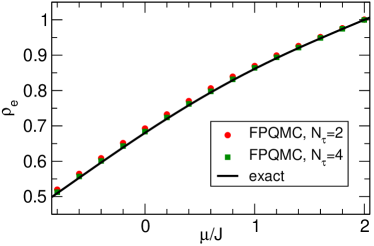
Figure 2: (Color online) Equation of state $\rho_{e}(\mu)$ for the Hubbard dimer with $T/J=1$, $U/J=4$. Full red circles (green squares) are the results of FPQMC simulations employing $N_{\tau}=2$ ($N_{\tau}=4$) imaginary-time slices, while the solid black line is computed using the exact diagonalization. The estimated statistical error of the FPQMC data is in all cases smaller than the symbol size.

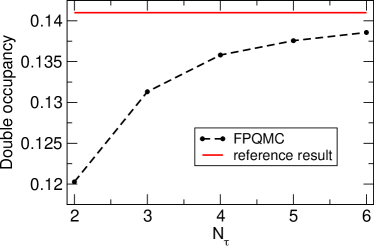
Figure 3: (Color online) Double occupancy of the $N_{c}=20$-site Hubbard chain at half-filling ($\mu=U/2$, $\rho_{e}=1$) as a function of the number $N_{\tau}$ of imaginary-time slices. The remaining parameters are $U/J=3$ and $T/J=1$. Dotted line connecting full symbols (FPQMC results) serves as a guide to the eye. Reference result is taken from Ref. 113. Relative deviation of the FPQMC result with $N_{\tau}=6$ from the reference result is around 2%. Statistical error bars of the FPQMC results are smaller than the symbol size.

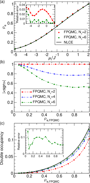
Figure 4: (Color online) (a) Equation of state $\rho_{e}(\mu)$ for the Hubbard model on a $4\times 4$ cluster with the following values of model parameters: $U/J=4$, $T/J=1.0408$. (b) The average sign as a function of the FPQMC estimate $\rho_{e,\mathrm{FPQMC}}$ of the electron density for different values of $N_{\tau}$. The dashed lines are guides to the eye. (c) The double occupancy $\sum_{\mathbf{r}}\langle n_{\mathbf{r}\uparrow}n_{\mathbf{r}\downarrow}\rangle/N_{c}$ as a function of the FPQMC estimate $\rho_{e,\mathrm{FPQMC}}$ of the electron density for different values of $N_{\tau}$. In (a) and (c), full symbols represent FPQMC results, the solid line shows the NLCE data taken from Ref. 41, while the insets show the relative deviation of FPQMC results from the reference NLCE results. The estimated statistical error of the FPQMC data is in all cases smaller than the symbol size.

We now apply the FPQMC method to evaluate the equation of state on larger clusters. We focus on a $4\times 4$ cluster, which may already be representative of the thermodynamic limit at $T/J\gtrsim 1$. [50] We compare our $\rho_{e}(\mu)$ results with the results of the numerical linked-cluster expansion (NLCE) method. [40, 41, 42] The NLCE results are numerically exact and converged with respect to the control parameter, i.e., the maximal cluster-size used. NLCE is commonly used to benchmark methods and understand experimental data. [9, 10] Again, we keep $U/J=4$, but we take $T/J=1.0408$ to be able to compare results to the data of Ref. 41. Figure 4(a) reveals that the FPQMC results with only $N_{\tau}=2$ imaginary-time slices agree very well (within a couple of percent) with the NLCE results over a wide range of chemical potentials. This is a highly striking observation, especially keeping in mind that the FPQMC method with $N_{\tau}=2$ is sign-problem-free, see Fig. 4(b). It is unclear whether other STD-based methods would reach here the same level of accuracy with only two imaginary-time slices (and without sign problem). This may be a specific property of the FPQMC method. Finer imaginary-time discretization introduces the sign problem, see Fig. 4(b), which becomes more pronounced as the density is increased and reaches a plateau for $\rho_{e}\gtrsim 0.8$. Still, the sign problem remains manageable. Increasing $N_{\tau}$ for 2 to 6 somewhat improves the agreement of the density $\rho_{e}$ [the inset of Fig. 4(a)] and considerably improves the agreement of the double occupancy [Fig. 4(c)] with the referent NLCE results. Still, comparing the insets of Figs. 4(a) and 4(c), we observe that the agreement between FPQMC ($N_{\tau}=6$) and NLCE results for $\rho_{e}$ is significantly better than for the double occupancy. The systematic error in FPQMC comes from the time-discretization and the finite size of the system. At $N_{\tau}=6$, it is not a priori clear which error contributes more, but it appears most likely that the time-discretization error is dominant. In any case, the reason why systematic error is greater for the double occupancy than for the average density could be that the double occupancy contains more detailed information about the correlations in the system. This might be an indication that measurement of multipoint density correlations will generally be more difficult—it may require a finer time resolution and/or greater lattice size.

The average sign above the half-filling $\rho_{e}=1$ mirrors that below the half-filling. The particle–hole symmetry ensures that $\rho_{e}(\mu)=2-\rho_{e}(U-\mu)$, but that it also governs the average sign is not immediately obvious from the construction of the method. A formal demonstration of the electron-doping–hole-doping symmetry of the average sign is, however, possible (see Appendix E). Note that we restrict our density calculations to $\rho_{e}<1$ because in this case the numerical effort to manipulate the determinants [Eqs. (7) and (10)] is lower (size of the corresponding matrices is given by the number of particles of a given spin). The performance of the FPQMC algorithm to compute $\rho_{e}(\mu)$ (average time needed to propose/accept an MC update and acceptance rates of individual MC updates) is discussed in Sec. SIII of the Supplementary Material.

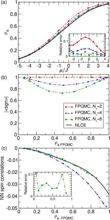
Figure 5: (Color online) (a) Equation of state $\rho_{e}(\mu)$ for the Hubbard model on a $4\times 4$ cluster with the following values of model parameters: $U/J=24$, $T/J=1.0408$. (b) The average sign as a function of the FPQMC estimate $\rho_{e,\mathrm{FPQMC}}$ of the electron density for different values of $N_{\tau}$. (c) Nearest-neighbor spin correlations $\sum_{\mathbf{r}\boldsymbol{\delta}}\langle S_{\mathbf{r}}^{z}S_{\mathbf{r}+\boldsymbol{\delta}}^{z}\rangle/N_{c}$ as a function of the FPQMC estimate $\rho_{e,\mathrm{FPQMC}}$ of the electron density for $N_{\tau}=4$ and 6. In (a) and (c), full symbols represent FPQMC results, the solid line shows the NLCE data taken from Ref. 41, while the insets show the relative deviation of FPQMC results from the reference NLCE results. The dashed or dash-dotted lines connecting the symbols serve as guides to the eye. The estimated statistical error of the FPQMC data is in all cases smaller than the symbol size.

We further benchmark our method in the case of very strong coupling, $U/J=24$ and, again, $T/J=1.0408$. Figure 5(a) compares the FPQMC results on a $4\times 4$ cluster using $N_{\tau}=2,4$, and 6 imaginary-time slices with the NLCE results. At extremely low fillings $\rho_{e}\lesssim 0.1$, the relative importance of the interaction term with respect to the kinetic term is quite small, and taking only $N_{\tau}=2$ suffices to reach a very good agreement between the FPQMC and NLCE results, see the inset of Fig. 5(a). As the filling is increased, the interaction effects become increasingly important, and it is necessary to increase $N_{\tau}$ in order to accurately describe the competition between the kinetic and interaction terms. In the inset of Fig. 5(a), we see that $N_{\tau}=6$ is sufficient to reach an excellent (within a couple of percent) agreement between FPQMC and NLCE results over a broad range of fillings. At very high fillings $\rho_{e}\gtrsim 0.9$ and for $N_{\tau}=6$, our MC updates that insert/remove particles have very low acceptance rates, which may lead to a slow sampling of the configuration space. It is for this reason that FPQMC results with $N_{\tau}=6$ do not significantly improve over $N_{\tau}=4$ results in this parameter regime. For $N_{\tau}=6$, an inefficient sampling near the half-filling also renders the corresponding results for the nearest-neighbor spin correlations $\sum_{\mathbf{r}\boldsymbol{\delta}}\langle S_{\mathbf{r}}^{z}S_{\mathbf{r}+\boldsymbol{\delta}}^{z}\rangle/N_{c}$ inaccurate, so that they are not displayed in Fig. 5(c). Here, vector $\boldsymbol{\delta}$ connects nearest-neighboring sites, while $S_{\mathbf{r}}^{z}=(n_{\mathbf{r}\uparrow}-n_{\mathbf{r}\downarrow})/2$ is the operator of $z$ projection of the local spin. At lower fillings $\rho_{e}\lesssim 0.8$, the agreement between our FPQMC results with $N_{\tau}=6$ and the NLCE results is good, while decreasing $N_{\tau}$ from 6 to 4 severely deteriorates the quality of the FPQMC results.

At this strong coupling, the dependence of the average sign on the density is somewhat modified, see Fig. 5(b). The minimal sign is no longer reached around half-filling but at quarter filling $\rho_{e}\sim 0.5$, around which $|\langle\mathrm{sgn}\rangle|$ appears to be symmetric. Comparing Fig. 5(b) to Fig. 4(b), we see that the average sign does not become smaller with increasing interaction, in sharp contrast with interaction-expansion-based methods such as CT-INT [32, 33] or configuration PIMC. [89]

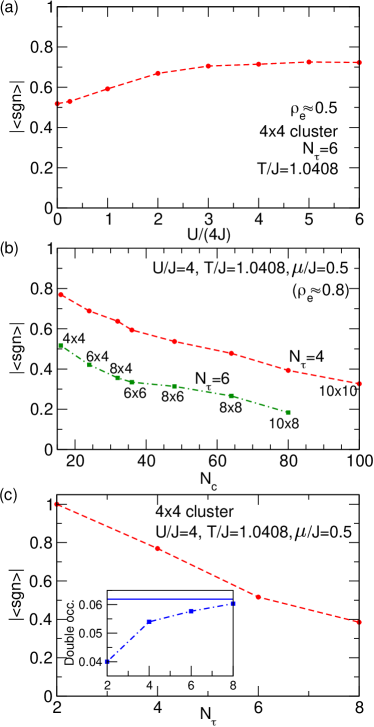
Figure 6: (Color online) (a) Average sign as a function of the ratio between the typical interaction and kinetic energies. Full symbols are results of FPQMC computations on a $4\times 4$ cluster with $N_{\tau}=6$, the temperature is fixed to $T/J=1.0408$, and the chemical potential at each $U$ is chosen such that $\rho_{e}\approx 0.5$. (b) Average sign as a function of the cluster size $N_{c}$ for the values of model parameters summarized in the figure. The FPQMC results (full symbols) are obtained using $N_{\tau}=4$ and 6. (c) Average sign as a function of $N_{\tau}$. The FPQMC results (full symbols) are obtained on a $4\times 4$ cluster for the values of model parameters summarized in the main part of the figure. The inset shows how the FPQMC result for double occupancy approaches the referent NLCE result as the imaginary-time discretization becomes finer.

To better understand the relation between the average sign and the interaction, in Fig. 6(a) we plot $|\langle\mathrm{sgn}\rangle|$ as a function of the ratio $U/(4J)$ of the typical interaction and kinetic energy. We take $N_{\tau}=6$ and adjust the chemical potential using the data from Ref. 41 so that $\rho_{e}\approx 0.5$. We see that $|\langle\mathrm{sgn}\rangle|$ monotonically increases with the interaction and reaches a plateau at very strong interactions. This is different from interaction-expansion-based QMC methods, whose sign problem becomes more pronounced as the interaction is increased. Also, for weak interactions, the performance of the FPQMC method deteriorates at high density, see Fig. 4(b), while methods such as CT-INT become problematic at low densities. The FPQMC method could thus become a method of choice to study the regimes of moderate coupling and temperature, which is highly relevant for optical-lattice experiments. Figure 6(b) shows the decrease of the average sign with the cluster size $N_{c}$ in the weak-coupling and moderate-temperature regime at filling $\rho_{e}\approx 0.8$. We observe that for both $N_{\tau}=4$ and $N_{\tau}=6$ the average sign decreases linearly with $N_{c}$. For $N_{\tau}=6$, we observe that the decrease for $N_{c}\lesssim 40$ is somewhat faster than the decrease for $N_{c}\gtrsim 40$. We, however, note that the acceptance rates of our MC updates strongly decrease with $N_{c}$ and that this decrease is more pronounced for finer imaginary-time discretizations. That is why we were not able to obtain any meaningful result for the $10\times 10$ cluster with $N_{\tau}=6$. At fixed cluster size and filling, the average sign decreases linearly with $N_{\tau}$, see the main part of Fig. 6(c), while the double occupancy tends to the referent NLCE value, see the inset of Fig. 6(c).

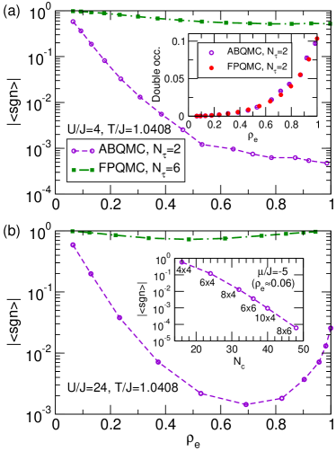
Figure 7: (Color online) Average sign as a function of the electron density in ABQMC simulations with $N_{\tau}=2$ (open circles) and FPQMC simulations with $N_{\tau}=6$ (full squares) for $T/J=1.0408$ and (a) $U/J=4$ and (b) $U/J=24$. The inset in panel (a) compares ABQMC (open circles) and FPQMC (full circles) results for the double occupancy as a function of $\rho_{e}$ (both methods employ $N_{\tau}=2$). The inset in panel (b) shows the average sign of ABQMC simulations with $N_{\tau}=2$ as a function of cluster size $N_{c}$ at low density ($\rho_{e}\approx 0.06,\mu/J=-5$).

In Sec. SIV of the Supplementary Material we provide an implementation of the ABQMC method in the equilibrium setup. Figures 7(a) and 7(b), which deal with the same parameter regimes as Figs. 4 and 5, respectively, clearly illustrate the advantages of the fermionic-propagator approach with respect to the alternating-basis approach in equilibrium. The average sign of ABQMC simulations with only 2 imaginary-time slices is orders of magnitude smaller than the sign of FPQMC simulations with three times finer imaginary-time discretization. Since FPQMC and ABQMC methods are related by an exact transformation, they should produce the same results for thermodynamic quantities (assuming that $N_{\tau}$ is the same in both methods). This is shown in the inset of Fig. 7(a) on the example of the double occupancy. The inset of Fig. 7(b) suggests that the average sign decreases exponentially with the cluster size $N_{c}$. Overall, our current implementation of the ABQMC method in equilibrium cannot be used to simulate larger clusters with a finer imaginary-time discretization.

III.2 Time-dependent results using FPQMC method: Local charge and spin densities

III.2.1 Benchmarks on small clusters

In Figs. 8(a) and 8(b) we benchmark our FPQMC method for time-dependent local densities on the example of the CDW state of the Hubbard tetramer, see the inset of Fig. 8(b). We follow the evolution of local charge densities on initially occupied sites for different ratios $U/D$, where $D$ is the half-bandwidth of the free-electron band ($D=2J$ for the tetramer). For all the interaction strengths considered, taking $N_{t}=2$ real-time slices on each branch (4 slices in total) is sufficient to accurately describe evolution of local densities up to times $Dt\sim 2$, see full symbols in Fig. 8(a). At longer times, $2<Dt\leq 4$, taking $N_{t}=3$ improves results obtained using $N_{t}=2$, compare empty to full symbols in Fig. 8(a). Nevertheless, for the strongest interaction considered ($U/D=1$), 6 real-time slices are not sufficient to bring the FPQMC result closer to the exact result at times $3\leq Dt\leq 4$. The average sign strongly depends on time and it drops by an order of magnitude upon increasing $N_{t}$ from 2 to 3, see Fig. 8(b). In spite of this, the discrepancy between the $N_{t}=3$ result and the exact result for $U/D=1$ cannot be ascribed to statistical errors, but to the systematic error of the FPQMC method (the minimum $N_{t}$ needed to obtain results with certain systematic error increases with both time and interaction strength).

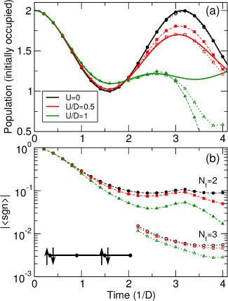
Figure 8: (Color online) (a) Time-dependent population of sites occupied in the initial CDW state of a tetramer for different interaction strengths. Solid lines represent exact results, full symbols connected by dashed lines are FPQMC results using $N_{t}=2$ real-time slices, while empty symbols connected by dotted lines are FPQMC results using $N_{t}=3$ real-time slices. The initial CDW state is schematically depicted in panel (b). (b) Time-dependent average sign of the FPQMC simulation using $N_{t}=2$ (full symbols connected by dashed lines) and $N_{t}=3$ (empty symbols connected by dotted lines) for different interaction strengths. In (a) and (b), FPQMC simulations using $N_{t}=3$ real-time slices are carried out only for $2<Dt\leq 4$.

III.2.2 Results on larger clusters

Figure 9: (Color online) (a) Time-dependent population of sites occupied in the initial CDW state of a $4\times 4$ cluster, which is schematically depicted in the inset of panel (b). FPQMC results using $N_{t}=2$ real-time slices (4 slices in total) are shown for five different interaction strengths (symbols) and compared with the noninteracting result (solid line). (b) Magnitude of the average sign as a function of time for different interaction strengths. Color code is the same as in panel (a). For $U/D=0.5,0.75,$ and 1 and $Dt\geq 1.2$, symbols ”$+$” and ”$-$” next to each point specify whether $\langle\mathrm{sgn}\rangle$ is positive or negative. (c) MC series for the population of initially occupied sites for $U/D=1$ and (c1) $Dt=1.2$, (c2) $Dt=1.4$, and (c3) $Dt=1.6$. (d) MC series for $\langle\mathrm{sgn}\rangle$ for $U/D=1$ and (d1) $Dt=1.2$, (d2) $Dt=1.4$, and (d3) $Dt=1.6$. Note the logarithmic scale on the abscissa in (c) and (d).

Figure 9(a) summarizes the evolution of local charge densities on initially occupied sites of a half-filled $4\times 4$ cluster, on which the electrons are initially arranged as depicted in the inset of Fig. 9(b). This state is representative of a CDW pattern formed by applying strong external density-modulating fields with wave vector $\mathbf{q}=(\pi,0)$. The FPQMC method employs 4 real-time slices in total, i.e., the forward and backward branch are divided into $N_{t}=2$ identical slices each. On the basis of the $N_{t}=2$ results in Fig. 8(a), we present the FPQMC dynamics up to maximum time $Dt_{\mathrm{max}}=2$. The extent of the dynamical sign problem is shown in Fig. 9(b).

At shortest times, $Dt\lesssim 1$, the results for all the interactions considered do not significantly differ from the noninteracting result. The same also holds for the average sign. As expected, the decrease of $|\langle\mathrm{sgn}\rangle|$ with time becomes more rapid as the interaction $U$ and time discretization $\Delta t=t/N_{t}$ are increased. The oscillatory nature of $\langle\mathrm{sgn}\rangle$ as a function of time [see Eq. 22] is correlated with the discontinuities in time-dependent populations observed in Fig. 9(a) for $U/D\geq 0.5$. Namely, at shortest times and for all the interactions considered, $\langle\mathrm{sgn}\rangle$ is positive, while for sufficiently strong interactions it becomes negative at longer times. This change is indicated in Fig. 9(b) by placing symbols ”$+$” and ”$-$” next to each relevant point. We now see that the discontinuities in populations occur precisely around instants at which $\langle\mathrm{sgn}\rangle$ turns from positive to negative values. Focusing on $U/D=1$, in Figs. 9(c1)–9(c3) we show MC series for the population of initially occupied sites at instants before [(c1)] and after [(c2), (c3)] $\langle\mathrm{sgn}\rangle$ passes through zero. The corresponding series for $\langle\mathrm{sgn}\rangle$ are presented in Figs. 9(d1)–9(d3). Well before [Figs. 9(c1) and 9(d1)] and after [Figs. 9(c3) and 9(d3)] $\langle\mathrm{sgn}\rangle$ changes sign, the convergence with the number of MC steps is excellent, while it is somewhat slower close to the positive-to-negative transition point, see Figs. 9(c2) and 9(d2). Still, the convergence at $Dt=1.4$ cannot be denied, albeit the statistical error of the population is larger than at $Dt=1.2$ and 1.6. At longer times $Dt\geq 1.5$, when $\langle\mathrm{sgn}\rangle$ is negative and of appreciable magnitude, the population again falls in the physical range $[0,2]$. Nevertheless, at such long times, the systematic error may be large due to the coarse real-time discretization.

In Sec. SV of the Supplementary Material we discuss FPQMC results for the dynamics of local charge densities starting from some other initial states.

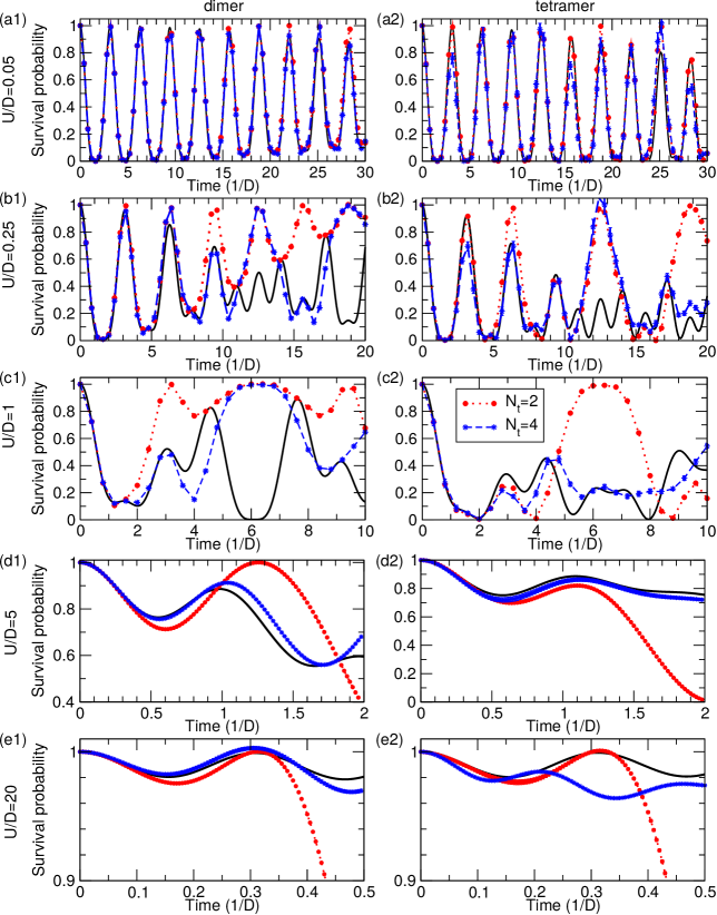
Figure 10: (Color online) Time dependence of the survival probability of the initial state $|\psi_{\mathrm{CDW}}\rangle$ or $|\psi_{\mathrm{SDW}}\rangle$ (see Table 1) for the dimer [(a1)–(e1)] and tetramer [(a2)–(e2)] for five different interaction strengths starting from the noninteracting limit and approaching the atomic limit: $U/D=0.05$ [(a1) and (a2)], $U/D=0.25$ [(b1) and (b2)], $U/D=1$ [(c1) and (c2)], $U/D=5$ [(d1) and (d2)], and $U/D=20$ [(e1) and (e2)]. The ABQMC results with $N_{t}=2$ (red full circles) and $N_{t}=4$ (blue stars) are compared with the exact result (black solid lines). The dotted/dashed lines connecting subsequent circles/stars are guides to the eye. In most cases, the MC error bars are smaller than the linear size of the symbols.

III.3 Time-dependent results using ABQMC method: Survival probability

III.3.1 Benchmarks on small clusters

We first benchmark our ABQMC method for the survival probability on Hubbard dimers and tetramers. The initial states are schematically summarized in Table 1. In both cases, we are at half-filling.

system	$|\psi_{\mathrm{CDW}}\rangle$	$|\psi_{\mathrm{SDW}}\rangle$
dimer
tetramer

Table 1: Schematic representations of the initial states of small systems on which the ABQMC method for $P(t)$ is benchmarked.

Figures 10(a1)–10(e2) present time evolution of the survival probability of the initial CDW-like and SDW-like states depicted in Table 1 for the dimer (left panels, $D=J$) and tetramer (right panels, $D=2J$) for different values of $U/D$ starting from the limit of weakly nonideal gas ($U/D=0.05$) and approaching the atomic limit ($U/D=20$). The results are obtained using $N_{t}=2$ (full red circles) and $N_{t}=4$ (blue stars) real-time slices and contrasted with the exact result (solid black lines). The ABQMC results with $N_{t}=2$ agree both qualitatively (oscillatory behavior) and quantitatively with the exact result up to $t_{\mathrm{max}}\sim 1/U$. Increasing $N_{t}$ from 2 to 4 may help decrease the deviation of the ABQMC data from the exact result at later times. Even when finer real-time discretization does not lead to better quantitative agreement, it may still help the ABQMC method qualitatively reproduce gross features of the exact result. The converged values of $|\langle\mathrm{sgn}\rangle|$ for the dimer and tetramer for $N_{t}=2,3,4$ are summarized in Table 2. For the dimer, increasing $N_{t}$ by one reduces $|\langle\mathrm{sgn}\rangle|$ by a factor of 2. In contrast, in the case of the tetramer, increasing $N_{t}$ by one reduces $|\langle\mathrm{sgn}\rangle|$ by almost an order of magnitude.

system	$N_{t}=2$	$N_{t}=3$	$N_{t}=4$
dimer	1/2	1/4	1/8
tetramer	1/8	$2.4\times 10^{-2}$	$3\times 10^{-3}$

Table 2: Modulus of the average sign for ABQMC simulations of $P(t)$ on dimer and tetramer with $N_{t}=2,3,$ and 4.

III.3.2 Results on larger clusters

We move on to discuss the survival-probability dynamics of different 16-electron and 8-electron states on a $4\times 4$ cluster. Figures 11(a) and 11(b) present $P(t)$ for 16-electron states schematically depicted in their respective insets. These states are representative of CDW patterns formed by applying strong external density-modulating fields with wave vectors $\mathbf{q}=(\pi,0)$ in Fig. 11(a) and $\mathbf{q}=(\pi,\pi)$ in Fig. 11(b). Figures 11(c) and 11(d) present $P(t)$ for 8-electron states schematically depicted in their respective insets. The ABQMC method employs $N_{t}=2$ real-time slices. The results are shown up to the maximum time $Dt_{\mathrm{max}}=2.5$, which we chose on the basis of the results presented in Fig. 10(c2).

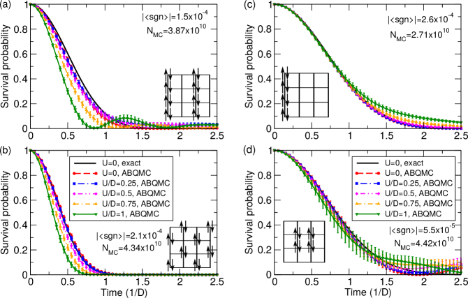
Figure 11: (Color online) Survival-probability dynamics of the 16-electron states [in (a) and (b)] and 8-electron states [in (c) and (d)] that are schematically depicted in the respective insets. ABQMC results are shown for five different interaction strengths (symbols) and compared with the noninteracting result (solid line). We cite the converged value of the average sign $|\langle\mathrm{sgn}\rangle|$, as well as the total number $N_{\mathrm{MC}}$ of MC steps completed.

As a sensibility check of our ABQMC results, we first compare the exact result in the noninteracting limit, see solid lines in Figs. 11(a)–11(d), with the corresponding ABQMC prediction, see full circles in Figs. 11(a)–11(d). While the exact and ABQMC result agree quite well in Figs. 11(b) and 11(c), the agreement in Figs. 11(a) and 11(d) is not perfect. Since no systematic errors are expected in ABQMC at $U=0$, the discrepancy must be due to statistical error. We confirm this expectation in Fig. 12 where we see that the obtained curve tends to the exact one with the increasing number of MC steps. The average sign cited in Fig. 11(d) suggests that more MC steps are needed to obtain fully converged results. Even though the converged average sign in Figs. 11(a)–11(c) is of the same order of magnitude, we find that the rate of convergence depends on both the number and the initial configuration of electrons.

In Figs. 11(a)–11(d), we observe that weak interactions ($U/D\lesssim 0.5$) do not cause any significant departure of $P(t)$ from the corresponding noninteracting result. On the other hand, the effect of somewhat stronger interactions on $P(t)$ depends crucially on the filling. In the 16-electron case, the increasing interactions speed up the initial decay of $P$, see Figs. 11(a) and 11(b), while in the 8-electron case interactions have little effect at $Dt<1$, see Figs. 11(c) and 11(d). This we attribute to the essential difference in the overall electron density and the relative role of the interaction term in the Hamiltonian. In the 16-electron case, starting from the moderate coupling $U/D\sim 1$, there is a clear revival of the initial state in Fig. 11(a), while no such a revival is observed in Fig. 11(b). Furthermore, the memory loss of the initial density-wave pattern is more rapid in Fig. 11(a) than in Fig. 11(b), even at $U=0$. The revival of the inital state is observed in the 8-electron case as well: at $t<1/D$ there is barely any effect of the interaction, yet at longer times it boosts $P$. However, in contrast to the 16-electron case, the results in Figs. 11(c) and 11(d) exhibit a weaker dependence of the survival-probability dynamics on the initial density-wave pattern. Indeed, the exact results in the noninteracting case are identical for both patterns in Figs. 11(c) and 11(d). Except in the case of the $(\pi,\pi)$ wave, the interactions lead to a persistence of the initial pattern at longer times, $t>1/D$. The precise form of temporal correlations that develop due to interactions apparently depends on the initial spatial arrangement of the electrons.

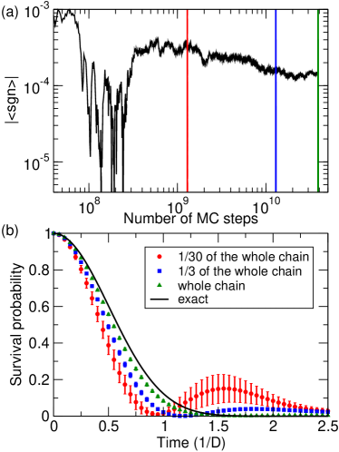
Figure 12: (Color online) (a) Average sign as a function of the number of MC steps in the ABQMC simulation of $P(t)$ for the 16-electron initial state schematically depicted in Fig. 11(a). (b) Time dependence of the survival probability for $U=0$ extracted using the first $1/30$ of the total number of MC steps completed ($1.29\times 10^{9}$ steps, full red circles), the first $1/3$ of the total number of MC steps completed ($1.29\times 10^{10}$ steps, full blue squares), and all the MC steps completed ($3.87\times 10^{10}$ steps, full green up-triangles). These results are compared to the exact result in the noninteracting limit, which are represented by the solid line. The vertical lines in (a), whose colors match the colors of the symbols in (b), denote the ending points of the simulations.

Section SVI of the Supplementary Material presents additional ABQMC results for the time-dependent survival probability.

IV Relation to other algorithms

As mentioned in the Introduction, a variant of the FPQMC method was first proposed by De Raedt and Lagendijk in 1980s. [78, 79, 80] They, however, explicitly retain permutation operators appearing in Eq. (41) in their final expression for $Z$, see, e.g., Eq. (3) in Ref. 78 or Eqs. (4.13) and (4.14) in Ref. 80. On the other hand, we analytically perform summation over permutation operators, thus grouping individual contributions into determinants. This is much more efficient [as factorial number of terms is captured in only $O(N^{3})$ steps, or even faster] and greatly improves the average sign (cancellations between different permutations are already contained in the determinant, see Fig. 7). The approach followed by De Raedt and Lagendijk later became known as permutation-sampling QMC, and the route followed by us is known as antisymmetric-propagator QMC, [85, 86] permutation-blocking QMC, [90] or fermionic-propagator QMC. [96] The analytical summation over permutation operators entering Eq. (41) was first performed by Takahashi and Imada. [85]

Our FPQMC method employs the lowest-order STD [Eq. (4)], which was also used in the permutation-sampling QMC method of De Raedt and Lagendijk. [78, 79, 80] The maximum number of imaginary-time slices $N_{\tau}$ they could use was limited by the acceptance rates of MC updates, which decrease quickly with increasing $N_{\tau}$ and the cluster size $N_{c}$. In our present implementation of FPQMC, we encounter the same issue, and our sampling becomes prohibitively inefficient when the total number of time slices is greater than 6–8, depending on the cluster size. To circumvent this issue, the fermionic-propagator idea was combined with higher-order STDs [98, 114, 115, 116] and more advanced sampling techniques [117, 118] to simulate equilibrium properties of continuum models of interacting fermions in the canonical [90, 92] and grand-canonical [96] ensemble. More recent algorithmic developments enabled simulations with as much as 2000 imaginary-time slices, [119] which is a great improvement. Whether similar ideas can be applied to lattice systems to improve the efficiency of sampling is currently unclear. Generally, more sophisticated STD schemes have been regarded as not useful in lattice-model applications. [120] It is important to note that the success of the antisymmetric-propagator algorithms in continuous systems relies on weak degeneracy. This corresponds to extremely low occupancy regime in lattice models, and it is precisely in this regime that our FPQMC method has the average sign close to 1 [see Figs. 4(b) and 5(b)], and the sampling is most efficient [see Sec. SIII of the Supplementary Material]. Near half-filling, lattice models present a fundamentally different physics, which may ultimately require a substantially different algorithmic approach.

We further emphasize that the low acceptance rates and the resulting inefficiency of sampling that we encounter is directly related to the discrete nature of space in our model. Some strategies for treating the analogous problem in continuous-space models may not be applicable here. For example, in continuous-space models, acceptance rates of individual updates can be adjusted by moving electrons over shorter distances, so that the new configuration weight is less likely to be substantially different from the old one. In contrast, in lattice models, electronic coordinates are discrete, and the minimum distance the electrons may cover is set by the lattice constant; In most cases moving a single electron by a single lattice spacing in a single time slice is sufficient to drastically reduce the configuration weight. There is no general rule on how electrons should be moved to ensure that the new configuration weight is close to the original one. This is particularly true for the updates that insert/remove a particle, and the problem becomes more pronounced with increasing $N_{\tau}$. When each of the $N_{\tau}$ states $|\Psi_{i,l}\rangle$ [see Eq. (9)] is changed to $|\Psi^{\prime}_{i,l}\rangle$, the chances that at least one of $\langle\Psi^{\prime}_{i,l\oplus 1}|e^{-\Delta\tau H_{0}}|\Psi^{\prime}_{i,l}\rangle$ is much smaller than $\langle\Psi_{i,l\oplus 1}|e^{-\Delta\tau H_{0}}|\Psi_{i,l}\rangle$ [see Eq. (10)] increase with $N_{\tau}$. Our configuration weight is appreciable only in small mutually disconnected regions of the configuration space, the movement between which is difficult. In Sec. V, we touch upon possible strategies to improve sampling of such a structured configuration space.

It is also important to compare our methods to the HF QMC method, [24, 49] which is a well-established STD-based method for the treatment of the Hubbard model. The HF method is manifestly sign-problem-free, but only at particle–hole symmetry. The sign problem can become severe away from half-filling, or on lattices other than the simple square lattice with no longer-range hoppings. On the other hand, our FPQMC method is nearly sign-problem-free at low occupancy, but also near the half-filling, albeit only at strong coupling [see Figs. 4(b) and 5(b)]. The other important difference is that matrices manipulated in HF are of the size $N_{c}N_{\tau}$, while in FPQMC, the matrices are of the size $<2N_{c}$, i.e., given by the number of particles. Algorithmic complexity of the individual MC step in FPQMC scales only linearly with $N_{\tau}$, while in HF, the MC step may go as $O(N_{\tau}^{2})$ [determinant is $O(N^{3})$, but fast updates $O(N^{2})$ are possible when the determinant is not calculated from scratch [49]]. Low cost of individual steps in FPQMC has allowed us to perform as many as $\sim 10^{10}$ MC steps in some calculations. This advantage, however, weighs against an increased configuration space to be sampled. In HF the number of possible configurations is $2^{N_{c}N_{\tau}}$ (space is spanned by $N_{c}N_{\tau}$ auxiliary Ising spins), while in FPQMC it is $4^{N_{c}N_{\tau}}$ (although, symmetries can be used to significantly reduce the number of possible configurations). The ABQMC method manipulates matrices of the same size as does FPQMC, but twice the number, and the configuration space is a priori even bigger ($16^{N_{c}N_{\tau}}$). Our methods also have a technical advantage that the measurements of multipoint charge and spin correlation functions are algorithmically trivial and cheap. Especially in ABQMC, the densities in both coordinate and momentum space can be simply read off the configuration. This is not possible in HF where the auxiliary Ising spin only distinguishes between singly-occupied and doubly-occupied/empty site. Most importantly, the ABQMC/FPQMC methods can be readily applied to canonical ensembles and pure states, which may not be possible with the HF method. However, the HF is commonly used with tens of time slices, for lattice sizes of order $N_{c}=100-200$; in FPQMC, algorithmic developments related to configuration updates are necessary before it can become a viable alternative to HF in any wide range of applications.

Finally, we are unaware of any numerically exact method for large lattice systems which can treat the full Kadanoff–Baym–Keldysh contour, and yield real-time correlation functions. Our ABQMC method represents an interesting example of a real-time QMC method with manifestly no dynamical sign problem. However, the average sign is generally poor. To push ABQMC to larger number of time slices (as needed for calculation of the time-dependence of observables) and lattices larger than $4\times 4$ will require further work, and most likely, conceptually new ideas.

V Summary and outlook

We revisit one of the earliest proposals for a QMC treatment of the Hubbard model, namely the permutation-sampling QMC method developed in Refs. 78, 79, 80. Motivated by recent progress in the analogous approach to continuous space models, we group all permutations into a determinant, which is known as the antisymmetric-propagator, [85] permutation-blocking, [90] fermionic-propagator [96] idea. We devise and implement two slightly different QMC methods. Depending on the details of the STD scheme, we distinguish between (1) the FPQMC method, where snapshots are given by real-space Fock states, and determinants represent antisymmetric propagators between those states, and (2) the ABQMC method, where slices alternate between real and reciprocal space representation, and determinants are simple Slater determinants. We thoroughly benchmark both methods against the available numerically exact data, and then use ABQMC to obtain some new results in the real-time domain.

The FPQMC method exhibits several promising properties. The average sign can be close to 1, and does not drop off rapidly with either the size of the system, or the number of time slices. In 1D, the method appears to be sign-problem-free. At present, the limiting factor is not the average sign, but the ability to sample the large configuration space. At discretizations finer than $N_{\tau}=6-8$, further algorithmic developments are necessary. Nevertheless, our calculations show that excellent results for instantaneous correlators can be obtained with very few time slices, and efficiently. Average density, double occupancy, and antiferromagnetic correlations can already be computed with high accuracy, at temperature and coupling strengths relevant for optical-lattice experiments. The FPQMC method is promising for further applications in equilibrium setups. In real-time applications, however, the sign problem in FPQMC is severe.

On the other hand, the ABQMC method has a significant sign problem in equilibrium applications, yet has some advantages in real-time applications. In ABQMC, the sign problem is manifestly time-independent, and calculations can be performed for multiple times and coupling strengths with a single Markov chain. We use this method to compute time-dependent survival probabilities of different density modulated states and identify several trends. The relevant transient regime is short, and, based on benchmarks, we estimate the systematic error due to the time discretization here to be small. Our results reveal that interactions speed up the initial decay of the survival probability, but facilitate a persistence of the initial charge-pattern at longer times. Additionally, we observe a characteristic value of the coupling constant, $U\sim 0.5D$, below which the interaction makes no visible effect on time-evolution. These findings bare qualitative predictions for future ultracold-atom experiments, but are limited to dynamics at the shortest wave-lengths, as dictated by the maximal size of the lattice that we can treat. We finally note that, within the ABQMC method, uniform currents, which are diagonal in the momentum representation, may be straightforwardly treated.

There is room for improvements in both the ABQMC and FPQMC methods. We already utilize several symmetries of the Hubbard model to improve efficiency and enforce some physical properties of solutions, but more symmetries can certainly be uncovered in the configuration spaces. Further grouping of configurations connected by symmetries can be used to alleviate some of the sign problem or improve efficiency. Also, sampling schemes may be improved along the lines of the recently proposed many-configuration Markov-chain MC, which visits an arbitrary number of configurations at every MC step. [121] Moreover, a better insight in the symmetries of the configuration space may make a deterministic, structured sampling (along the lines of quasi-MC methods [122, 123, 124]) superior to the standard pseudo-random sampling.

Supplementary Material

See the supplementary material for (i) a detailed description of MC updates within the FPQMC method, (ii) a detailed description of MC updates within the ABQMC method for time-dependent survival probability, (iii) details on the performance of the FPQMC method in equilibrium calculations, (iv) discussion on the applicability of the ABQMC method in equilibrium calculations, (v) additional FPQMC calculations of time-dependent local densities, (vi) additional ABQMC calculations of time-dependent survival probability, and (vii) formulation and benchmarks of ABQMC method in quench setups (on the full three-piece Kadanoff–Baym–Keldysh contour).

Authors’ Contributions

J.V. conceived the research. V.J. developed the formalism and computational codes under the guidance of J.V., conducted all numerical simulations, analyzed their results, and prepared the initial version of the manuscript. Both authors contributed to the submitted version of the manuscript.

Data availability

The data that support the findings of this study are available from the corresponding author upon reasonable request.

Appendix A Many-body propagator as a determinant of single-particle propagators

The demonstration of Eqs. (6) and (7) can be conducted for each spin component separately. We thus fix the spin index $\sigma$ and further omit it from the definition of the many-fermion state $|\Psi_{i}\rangle$ [Eq. (5)]. Since $H_{0}$ is diagonal in the momentum representation, we express the state $|\Psi_{i}\rangle$ in the momentum representation

$$|\Psi_{i}\rangle=\sum_{\{\mathbf{k}_{j}\}}\left(\prod_{l=1}^{N}\langle\mathbf{k}_{l}|\mathbf{r}_{l}\rangle c_{\mathbf{k}_{l}}^{\dagger}\right)|\emptyset\rangle$$ (37)

and similarly for $|\Psi^{\prime}_{i}\rangle$. While the positions $\mathbf{r}_{1},\dots,\mathbf{r}_{N}$ are ordered according to a certain rule, the wave vectors $\mathbf{k}_{1},\dots,\mathbf{k}_{N}$ entering Eq. (37) are not ordered, and there is no restriction on the sum over them. We have

$$\begin{split}\langle\Psi^{\prime}_{i}|e^{-\Delta\alpha H_{0}}|\Psi_{i}\rangle=&\sum_{\{\mathbf{k}^{\prime}_{l}\}}\sum_{\{\mathbf{k}_{l}\}}e^{-\Delta\alpha\varepsilon_{\mathbf{k}_{1}}}\dots e^{-\Delta\alpha\varepsilon_{\mathbf{k}_{N}}}\times\\ &\langle\mathbf{r}^{\prime}_{N}|\mathbf{k}^{\prime}_{N}\rangle\dots\langle\mathbf{r}^{\prime}_{1}|\mathbf{k}^{\prime}_{1}\rangle\langle\mathbf{k}_{1}|\mathbf{r}_{1}\rangle\langle\mathbf{k}_{N}|\mathbf{r}_{N}\rangle\times\\ &\langle\emptyset|c_{\mathbf{k}^{\prime}_{N}}\dots c_{\mathbf{k}^{\prime}_{1}}c_{\mathbf{k}_{1}}^{\dagger}\dots c_{\mathbf{k}_{N}}^{\dagger}|\emptyset\rangle.\end{split}$$ (38)

The sums over $\{\mathbf{k}^{\prime}_{l}\}$ are eliminated by employing the identity [80]

$$\begin{split}&\langle\emptyset|c_{\mathbf{k}^{\prime}_{N}}\dots c_{\mathbf{k}^{\prime}_{1}}c_{\mathbf{k}_{1}}^{\dagger}\dots c_{\mathbf{k}_{N}}^{\dagger}|\emptyset\rangle=\\ &\sum_{\mathcal{P}}\mathrm{sgn}(\mathcal{P})\>\delta(\mathbf{k}^{\prime}_{1},\mathbf{k}_{\mathcal{P}(1)})\dots\delta(\mathbf{k}^{\prime}_{N},\mathbf{k}_{\mathcal{P}(N)})\end{split}$$ (39)

where the permutation operator $\mathcal{P}$ acts on the set of indices $\{1,\dots,N\}$, while $\mathrm{sgn}(\mathcal{P})=\pm 1$ is the permutation parity. We then observe that

$$\prod_{l=1}^{N}\langle\mathbf{r}^{\prime}_{l}|\mathbf{k}_{\mathcal{P}(l)}\rangle=\prod_{l=1}^{N}\langle\mathbf{r}^{\prime}_{\mathcal{P}^{-1}(l)}|\mathbf{k}_{l}\rangle,$$ (40)

which permits us to perform the sums over individual $\mathbf{k}_{l}$s independently. Combining Eqs. (38)–(40) and changing the permutation variable $\mathcal{P}^{\prime}=\mathcal{P}^{-1}$ we eventually obtain

$$\begin{split}\langle\Psi^{\prime}_{i}|e^{-\Delta\alpha H_{0}}|\Psi_{i}\rangle&=\sum_{\mathcal{P}^{\prime}}\mathrm{sgn}(\mathcal{P}^{\prime})\prod_{l=1}^{N}\langle\mathbf{r}^{\prime}_{\mathcal{P}^{\prime}(l)}|e^{-\Delta\alpha H_{0}}|\mathbf{r}_{l}\rangle\\ &=\det S(\Psi^{\prime}_{i},\Psi_{i},\Delta\alpha)\end{split}$$ (41)

where matrix $S(\Psi^{\prime}_{i},\Psi_{i},\Delta\alpha)$ (here without the spin index) is defined in Eq. (7).

Appendix B Propagator of a free particle on the square lattice

Here, we provide the expressions for the propagator of a free particle on the square lattice in imaginary [$\Delta\alpha=\Delta\tau$ in Eq. (7)] and real [$\Delta\alpha=i\Delta t$ in Eq. (7)] time. In imaginary time,

$$\langle\mathbf{r}^{\prime}|e^{-\Delta\tau H_{0}}|\mathbf{r}\rangle=\mathcal{I}(2J\Delta\tau,r^{\prime}_{x}-r_{x})\mathcal{I}(2J\Delta\tau,r^{\prime}_{y}-r_{y})$$ (42)

where the one-dimensional imaginary-time propagator ($l$ is an integer)

$$\mathcal{I}(z,l)=\frac{1}{N}\sum_{j=0}^{N-1}\cos\left(\frac{2\pi jl}{N}\right)\exp\left(z\cos\left(\frac{2\pi j}{N}\right)\right)$$ (43)

is related to the modified Bessel function of the first kind $I_{l}(z)$ via

$$\lim_{N\to\infty}\mathcal{I}(z,l)=\frac{1}{\pi}\int_{0}^{\pi}d\theta\>\cos(l\theta)\>e^{z\cos\theta}=I_{l}(z).$$ (44)

In real time,

$$\langle\mathbf{r}^{\prime}|e^{-i\Delta tH_{0}}|\mathbf{r}\rangle=\mathcal{J}(2J\Delta t,r^{\prime}_{x}-r_{x})\mathcal{J}(2J\Delta t,r^{\prime}_{y}-r_{y})$$ (45)

where the one-dimensional real-time propagator ($l$ is an integer)

$$\mathcal{J}(z,l)=\frac{1}{N}\sum_{j=0}^{N-1}\cos\left(\frac{2\pi jl}{N}\right)\exp\left(iz\cos\left(\frac{2\pi j}{N}\right)\right)$$ (46)

is related to the Bessel function of the first kind $J_{l}(z)$ via

$$\lim_{N\to\infty}\mathcal{J}(z,l)=\frac{1}{\pi}\int_{0}^{\pi}d\theta\>\cos(l\theta)\>e^{iz\cos\theta}=i^{l}J_{l}(z).$$ (47)

For finite $N$, $\mathcal{J}(z,2l)$ is purely real, while $\mathcal{J}(z,2l+1)$ is purely imaginary.

Appendix C Derivation of the FPQMC formulae that manifestly respect the dynamical symmetry of the Hubbard model

Here, we derive the FPQMC expression for the time-dependent expectation value of a local observable [Eq. (18)] that manifestly respects the dynamical symmetry of the Hubbard model.

We start by defining the operation of the bipartite lattice symmetry, which is represented by a unitary, hermitean, and involutive operator $B$ ($B^{\dagger}=B=B^{-1}$) whose action on electron creation and annihilation operators in the real space is given as

$$Bc_{\mathbf{r}\sigma}^{\left(\dagger\right)}B=(-1)^{r_{x}+r_{y}}c_{\mathbf{r}\sigma}^{\left(\dagger\right)}.$$ (48)

In the momentum space, $B$ is actually the so-called $\pi$-boost [15]

$$Bc_{\mathbf{k}\sigma}^{\left(\dagger\right)}B=c_{\mathbf{k}+\mathbf{Q},\sigma}^{\left(\dagger\right)}$$ (49)

that increases the electronic momentum by $\mathbf{Q}=(\pi,\pi)$. The time reversal operator $T$ is an antiunitary (unitary and antilinear), involutive, and hermitean operator whose action on electron creation and annihilation operators in the real space is given as

$$Tc_{\mathbf{r}\uparrow}^{\left(\dagger\right)}T=c_{\mathbf{r}\downarrow}^{\left(\dagger\right)},\quad Tc_{\mathbf{r}\downarrow}^{\left(\dagger\right)}T=-c_{\mathbf{r}\uparrow}^{\left(\dagger\right)},$$ (50)

while the corresponding relations in the momentum space read as

$$Tc_{\mathbf{k}\uparrow}^{\left(\dagger\right)}T=c_{-\mathbf{k}\downarrow}^{\left(\dagger\right)},\quad Tc_{\mathbf{k}\downarrow}^{\left(\dagger\right)}T=-c_{-\mathbf{k}\uparrow}^{\left(\dagger\right)}.$$ (51)

Using Eqs. (48)–(51), it follows that

$$BH_{0}B=-H_{0},\quad BH_{\mathrm{int}}B=H_{\mathrm{int}},\quad TH_{0}T=H_{0},\quad TH_{\mathrm{int}}T=H_{\mathrm{int}}.$$ (52)

In Sec. II.2.2, we assumed that the initial state $|\psi(0)\rangle$ is an eigenstate of local density operators $n_{\mathbf{r}\sigma}$, which means that $B|\psi(0)\rangle=e^{i\chi_{B}}|\psi(0)\rangle$, see Eq. (48).

The denominator of Eq. (18)

$$A_{\mathrm{den}}(t)=\langle\psi(0)|e^{iHt}\>e^{-iHt}|\psi(0)\rangle$$ (53)

is purely real, $A_{\mathrm{den}}(t)=A_{\mathrm{den}}(t)^{*}$, so that

$$\begin{split}A_{\mathrm{den}}(t)\approx&\frac{1}{2}\left\langle\psi(0)\left|\left(e^{iH_{0}\Delta t}e^{iH_{\mathrm{int}}\Delta t}\right)^{N_{t}}\left(e^{-iH_{0}\Delta t}e^{-iH_{\mathrm{int}}\Delta t}\right)^{N_{t}}\right|\psi(0)\right\rangle+\\ &\frac{1}{2}\left\langle\psi(0)\left|\left(e^{iH_{\mathrm{int}}\Delta t}e^{iH_{0}\Delta t}\right)^{N_{t}}\left(e^{-iH_{\mathrm{int}}\Delta t}e^{-iH_{0}\Delta t}\right)^{N_{t}}\right|\psi(0)\right\rangle.\end{split}$$ (54)

We thus obtain

$$A_{\mathrm{den}}(t)\approx\sum_{\mathcal{C}}\left\{\mathrm{Re}\{\mathcal{D}_{2t}(\mathcal{C},\Delta t)\}\cos[\Delta\varepsilon_{\mathrm{int}}(\mathcal{C})\Delta t]-\mathrm{Im}\{\mathcal{D}_{2t}(\mathcal{C},\Delta t)\}\sin[\Delta\varepsilon_{\mathrm{int}}(\mathcal{C})\Delta t]\right\},$$ (55)

where configuration $\mathcal{C}$ consists of $2N_{t}-1$ independent states $|\Psi_{i,2}\rangle,\dots,|\Psi_{i,2N_{t}}\rangle$, $|\Psi_{i,1}\rangle\equiv|\psi(0)\rangle$, while $\mathcal{D}_{2t}(\mathcal{C},\Delta t)$ and $\Delta\varepsilon_{\mathrm{int}}(\mathcal{C})$ are defined in Eqs. (21) and (20), respectively. The denominator is also invariant under time reversal, $A_{\mathrm{den}}(t)=A_{\mathrm{den}}(-t)$, which is not a consequence of a specific behavior of the initial state under time reversal, but rather follows from $A_{\mathrm{den}}(t)\equiv\langle\psi(0)|\psi(0)\rangle$. In other words, Eq. (55) should contain only contributions invariant under the transformation $\Delta t\to-\Delta t$. Using the bipartite lattice symmetry, under which $B|\Psi_{i,l}\rangle=e^{i\chi_{l}}|\Psi_{i,l}\rangle$, we obtain

$$\begin{split}\mathcal{D}_{2t}(\mathcal{C},-\Delta t)&=\prod_{l=N_{t}+1}^{2N_{t}}\langle\Psi_{i,l\oplus 1}|BBe^{-iH_{0}\Delta t}BB|\Psi_{i,l}\rangle\prod_{l=1}^{N_{t}}\langle\Psi_{i,l\oplus 1}|BBe^{iH_{0}\Delta t}BB|\Psi_{i,l}\rangle\\ &=\prod_{l=N_{t}+1}^{2N_{t}}\langle\Psi_{i,l\oplus 1}|e^{iH_{0}\Delta t}|\Psi_{i,l}\rangle\prod_{l=1}^{N_{t}}\langle\Psi_{i,l\oplus 1}|e^{-iH_{0}\Delta t}|\Psi_{i,l}\rangle=\mathcal{D}_{2t}(\mathcal{C},\Delta t).\end{split}$$ (56)

Equation (55) then reduces to

$$A_{\mathrm{den}}(t)=\sum_{\mathcal{C}}\mathrm{Re}\{\mathcal{D}_{2t}(\mathcal{C},\Delta t)\}\cos[\Delta\varepsilon_{\mathrm{int}}(\mathcal{C})\Delta t].$$ (57)

We now turn to the numerator of Eq. (18)

$$A_{\mathrm{num}}(t)=\langle\psi(0)|e^{iHt}\>A_{i}\>e^{-iHt}|\psi(0)\rangle,$$ (58)

which is also purely real, $A_{\mathrm{num}}(t)=A_{\mathrm{num}}(t)^{*}$, so that

$$A_{\mathrm{num}}(t)\approx\sum_{\mathcal{C}}\mathcal{A}_{i}(\Psi_{i,N_{t}+1})\left\{\mathrm{Re}\{\mathcal{D}_{2t}(\mathcal{C},\Delta t)\}\cos[\Delta\varepsilon_{\mathrm{int}}(\mathcal{C})\Delta t]-\mathrm{Im}\{\mathcal{D}_{2t}(\mathcal{C},\Delta t)\}\sin[\Delta\varepsilon_{\mathrm{int}}(\mathcal{C})\Delta t]\right\}.$$ (59)

In the following discussion, we assume that the time reversal operation changes $|\psi(0)\rangle$ by a phase factor, $T|\psi(0)\rangle=e^{i\chi_{T}}|\psi(0)\rangle$. This, combined with $B|\psi(0)\rangle=e^{i\chi_{B}}|\psi(0)\rangle$, gives the assumption on $|\psi(0)\rangle$ that is mentioned before Eq. (LABEL:Eq:A_a_ABMC_symmetry). We furthermore assume that $TBA_{i}BT=A_{i}$. Under these assumptions, the numerator is invariant under time reversal, $A_{\mathrm{num}}(-t)=A_{\mathrm{num}}(t)$, meaning that Eq. (59) should contain only contributions invariant under the transformation $\Delta t\to-\Delta t$. Using Eq. (56), Eq. (59) reduces to

$$A_{\mathrm{num}}(t)\approx\sum_{\mathcal{C}}\mathcal{A}_{i}(\Psi_{i,N_{t}+1})\>\mathrm{Re}\{\mathcal{D}_{2t}(\mathcal{C},\Delta t)\}\cos[\Delta\varepsilon_{\mathrm{int}}(\mathcal{C})\Delta t],$$ (60)

and Eq. (22) follows immediately.

An example of the initial state $|\psi(0)\rangle$ and the observable $A_{i}$ that satisfy $TB|\psi(0)\rangle=e^{i\chi}|\psi(0)\rangle$ and $TBA_{i}BT=A_{i}$ are the CDW state $|\psi_{\mathrm{CDW}}\rangle$ [Eq. (24)] and the local charge density $A_{i}=\sum_{\sigma}n_{\mathbf{r}\sigma}$. While the time-reversal operation may change a general SDW state [Eq. (23)] by more than a phase factor, Eq. (60) is still applicable when the observable of interest is the local spin density $A_{i}=n_{\mathbf{r}\uparrow}-n_{\mathbf{r}\downarrow}$. This follows from the transformation law $T(n_{\mathbf{r}\uparrow}-n_{\mathbf{r}\downarrow})T=n_{\mathbf{r}\downarrow}-n_{\mathbf{r}\uparrow}$ and the fact that the roles of spin-up and spin-down electrons in the state $T|\psi_{\mathrm{SDW}}\rangle$ are exchanged with respect to the state $|\psi_{\mathrm{SDW}}\rangle$.

We now explain how we use Eq. (LABEL:Eq:pops_cdw_sdw) to enlarge statistics in computations of time-dependent local spin (charge) densities when the evolution starts from state $|\psi_{\mathrm{SDW}}\rangle$ in Eq. (23) [$|\psi_{\mathrm{CDW}}\rangle$ in Eq. (24)]. Let us limit the discussion to the spin (charge) density at fixed position $\mathbf{r}$. Suppose that we obtained Markov chains (of length $N_{\mathrm{CDW}}$) $\{\mathcal{N}_{1}^{\mathrm{CDW}}(t),\dots,\mathcal{N}_{N_{\mathrm{CDW}}}^{\mathrm{CDW}}(t)\}$ and $\{\mathcal{D}_{1}^{\mathrm{CDW}},\dots,\mathcal{D}_{N_{\mathrm{CDW}}}^{\mathrm{CDW}}\}$ for the numerator and denominator. Suppose also that we obtained Markov chains (of length $N_{\mathrm{SDW}}$) $\{\mathcal{N}_{1}^{\mathrm{SDW}}(t),\dots,\mathcal{N}_{N_{\mathrm{SDW}}}^{\mathrm{SDW}}(t)\}$ and $\{\mathcal{D}_{1}^{\mathrm{SDW}},\dots,\mathcal{D}_{N_{\mathrm{SDW}}}^{\mathrm{SDW}}\}$ for the numerator and denominator. Using these Markov chains, we found that the best result for the time-dependent local spin (charge) density is obtained by joining them into one Markov chain $\{\mathcal{N}_{1}^{\mathrm{SDW}}(t),\dots,\mathcal{N}_{N_{\mathrm{SDW}}}^{\mathrm{SDW}}(t),\mathcal{N}_{1}^{\mathrm{CDW}}(t),\dots,\mathcal{N}_{N_{\mathrm{CDW}}}^{\mathrm{CDW}}(t)\}$ of length $N_{\mathrm{SDW}}+N_{\mathrm{CDW}}$ for the numerator, and another Markov chain $\{\mathcal{D}_{1}^{\mathrm{SDW}},\dots,\mathcal{D}_{N_{\mathrm{SDW}}}^{\mathrm{SDW}},\mathcal{D}_{1}^{\mathrm{CDW}},\dots,\mathcal{D}_{N_{\mathrm{CDW}}}^{\mathrm{CDW}}\}$ of length $N_{\mathrm{SDW}}+N_{\mathrm{CDW}}$ for the denominator. If individual chain lengths $N_{\mathrm{CDW}}$ and $N_{\mathrm{SDW}}$ are sufficiently large, the manner in which the chains are joined is immaterial; here, we append the CDW chain to the SDW chain, and we note that other joining possibilities lead to the same final result (within the statistical error bars). To further reduce statistical error bars, we also combine SDW+CDW chains at all positions $\mathbf{r}$ that have the same spin (charge) density by the symmetry of the initial state.

Appendix D Derivation of the ABQMC formula for the survival probability

We start from the survival-probability amplitude

$$A_{P}(t)=\frac{\langle\psi(0)|e^{-iHt}|\psi(0)\rangle}{\langle\psi(0)|\psi(0)\rangle}$$ (61)

whose numerator can be expressed as

$$\begin{split}\langle\psi(0)|e^{-iHt}|\psi(0)\rangle&\approx\frac{1}{2}\left\langle\psi(0)\left|\left(e^{-iH_{0}\Delta t}e^{-iH_{\mathrm{int}}\Delta t}\right)^{N_{t}}\right|\psi(0)\right\rangle+\frac{1}{2}\left\langle\psi(0)\left|\left(e^{-iH_{\mathrm{int}}\Delta t}e^{-iH_{0}\Delta t}\right)^{N_{t}}\right|\psi(0)\right\rangle\\ &=\sum_{\Psi_{i,2}\dots\Psi_{i,N_{t}}}\mathrm{Re}\left\{\prod_{l=1}^{N_{t}}\langle\Psi_{i,l\oplus 1}|e^{-iH_{0}\Delta t}|\Psi_{i,l}\rangle\right\}e^{-i\varepsilon_{\mathrm{int}}(\mathcal{C})\Delta t}\\ &=\sum_{\Psi_{i,2}\dots\Psi_{i,N_{t}}}\sum_{\Psi_{k,1}\dots\Psi_{k,N_{t}}}\mathrm{Re}\left\{\prod_{l=1}^{N_{t}}\langle\Psi_{i,l\oplus 1}|\Psi_{k,l}\rangle\langle\Psi_{k,l}|\Psi_{i,l}\rangle e^{-i\varepsilon_{0}(\mathcal{C})\Delta t}\right\}e^{-i\varepsilon_{\mathrm{int}}(\mathcal{C})\Delta t}\\ &=\sum_{\mathcal{C}}\left\{\mathrm{Re}\{\mathcal{D}(\mathcal{C})\}\cos[\varepsilon_{0}(\mathcal{C})\Delta t]+\mathrm{Im}\{\mathcal{D}(\mathcal{C})\}\sin[\varepsilon_{0}(\mathcal{C})\Delta t]\right\}e^{-i\varepsilon_{\mathrm{int}}(\mathcal{C})\Delta t}.\end{split}$$ (62)

In going from the second to the third line of Eq. (62), we introduced spectral decompositions of $N_{t}$ factors $e^{-iH_{0}\Delta t}$. The configuration $\mathcal{C}$ entering the last line of Eq. (62) consists of $N_{t}-1$ independent states $|\Psi_{i,2}\rangle,\dots,|\Psi_{i,N_{t}}\rangle$ in the coordinate representation and $N_{t}$ independent states $|\Psi_{k,1}\rangle,\dots,|\Psi_{k,N_{t}}\rangle$ in the momentum representation, while $|\Psi_{i,1}\rangle\equiv|\psi(0)\rangle$. $\mathcal{D}(\mathcal{C})$ and $\varepsilon_{0}(\mathcal{C})$ are defined in Eqs. (31) and (34), respectively. By virtue of the bipartite lattice symmetry, under which $\mathcal{D(\mathcal{C})}$ remains invariant, while $\varepsilon_{0}(\mathcal{C})$ changes sign, the summand containing $\sin[\varepsilon_{0}(\mathcal{C})\Delta t]$ in Eq. (62) vanishes, so that

$$\begin{split}\langle\psi(0)|e^{-iHt}|\psi(0)\rangle\approx\sum_{\mathcal{C}}\mathrm{Re}\{\mathcal{D}(\mathcal{C})\}\>\cos[\varepsilon_{0}(\mathcal{C})\Delta t]\>e^{-i\varepsilon_{\mathrm{int}}(\mathcal{C})\Delta t}.\end{split}$$ (63)

This form should be used, e.g., when $|\psi(0)\rangle$ is the SDW state defined in Eq. (23). When the initial state is the CDW state defined in Eq. (24), $T|\psi(0)\rangle=e^{i\chi_{T}}|\psi(0)\rangle$, $\langle\psi(0)|e^{-iHt}|\psi(0)\rangle$ is purely real, so that

$$\langle\psi(0)|e^{-iHt}|\psi(0)\rangle\approx\sum_{\mathcal{C}}\mathrm{Re}\{\mathcal{D}(C)\}\cos[\varepsilon_{0}(\mathcal{C})\Delta t]\cos[\varepsilon_{\mathrm{int}}(\mathcal{C})\Delta t].$$ (64)

Equation (30) then follows by combining Eq. (64) with $\langle\psi(0)|\psi(0)\rangle=\sum_{\mathcal{C}}\mathrm{Re}\{\mathcal{D}(\mathcal{C})\}$.

We now provide a formal demonstration of Eq. (LABEL:Eq:equal_P_t). The partial particle–hole transformation is represented by a unitary, hermitean, and involutive operator $P$ ($P^{\dagger}=P=P^{-1}$) whose action on electron creation and annihilation operators in the real space is given as [109, 110]

$$Pc_{\mathbf{r}\uparrow}P=c_{\mathbf{r}\uparrow},\quad Pc_{\mathbf{r}\uparrow}^{\dagger}P=c_{\mathbf{r}\uparrow}^{\dagger},$$ (65)

$$Pc_{\mathbf{r}\downarrow}P=(-1)^{r_{x}+r_{y}}c_{\mathbf{r}\downarrow}^{\dagger},\quad Pc_{\mathbf{r}\downarrow}^{\dagger}P=(-1)^{r_{x}+r_{y}}c_{\mathbf{r}\downarrow}.$$ (66)

The interaction Hamiltonian $H_{\mathrm{int}}$ thus transforms under the partial particle–hole transformation as $PH_{\mathrm{int}}P=U\widehat{N}_{\uparrow}-H_{\mathrm{int}}$. The action of the partial particle–hole transformation in the momentum space reads as [$\mathbf{Q}=(\pi,\pi)$]

$$Pc_{\mathbf{k}\uparrow}P=c_{\mathbf{k}\uparrow},\quad Pc_{\mathbf{k}\uparrow}^{\dagger}P=c_{\mathbf{k}\uparrow}^{\dagger},$$ (67)

$$Pc_{\mathbf{k}\downarrow}P=c_{\mathbf{Q}-\mathbf{k},\downarrow}^{\dagger},\quad Pc_{\mathbf{k}\downarrow}^{\dagger}P=c_{\mathbf{Q}-\mathbf{k},\downarrow}.$$ (68)

The kinetic energy, therefore, remains invariant under the partial particle–hole transformation, i.e., $PH_{0}P=H_{0}$. Equations (65) and (66) imply that $P|\emptyset\rangle=\prod_{\mathbf{r}\in\mathcal{U}}c_{\mathbf{r}\downarrow}^{\dagger}|\emptyset\rangle$. We then find that $P|\psi_{\mathrm{CDW}}\rangle=|\psi_{\mathrm{SDW}}\rangle$, i.e., the partial particle–hole transformation transforms the CDW state defined in Eq. (24) into the SDW state defined in Eq. (23) and vice versa. [108] The states $|\psi_{\mathrm{CDW}}\rangle$ and $|\psi_{\mathrm{SDW}}\rangle$ have the same number of spin-up electrons, while their numbers of spin-down electrons add to $N_{c}$. Using the combination of the partial particle–hole transformation $P$ and bipartite lattice transformation $B$ defined in Appendix C, one obtains

$$\langle\psi_{\mathrm{CDW}}|e^{-iHt}|\psi_{\mathrm{CDW}}\rangle=e^{-iN_{\uparrow}(\psi)Ut}\langle\psi_{\mathrm{SDW}}|e^{-iHt}|\psi_{\mathrm{SDW}}\rangle^{*},$$ (69)

where $N_{\uparrow}(\psi)=\langle\psi_{\mathrm{CDW}}|\widehat{N}_{\uparrow}|\psi_{\mathrm{CDW}}\rangle=\langle\psi_{\mathrm{SDW}}|\widehat{N}_{\uparrow}|\psi_{\mathrm{SDW}}\rangle$ is the total number of spin-up electrons in CDW and SDW states. Equation (LABEL:Eq:equal_P_t) then follows immediately from Eq. (69).

A similar procedure to that described in Appendix C is used to combine Markov chains for the survival probabilities of the CDW and SDW states related by the dynamical symmetry in Eq. (69).

Appendix E Using the particle–hole symmetry to discuss the average sign of the FPQMC method for chemical potentials $\mu$ and $U-\mu$

The (full) particle–hole transformation is represented by a unitary, hermitean, and involutive operator $P_{f}$ ($P_{f}^{\dagger}=P_{f}=P_{f}^{-1}$) whose action on electron creation and annihilation operators in the real space is defined as [109, 110]

$$P_{f}c_{\mathbf{r}\sigma}P_{f}=(-1)^{r_{x}+r_{y}}c_{\mathrm{r}\sigma}^{\dagger}.$$ (70)

The corresponding formula in the momentum space reads as

$$P_{f}c_{\mathbf{k}\sigma}P_{f}=c_{\mathbf{Q}-\mathbf{k},\sigma}^{\dagger}.$$ (71)

Let us fix $J,U,T$, and $N_{\tau}$ and compute the equation of state $\rho_{e}(\mu)$ using Eq. (13) in which $\mathcal{A}_{i}(\Psi_{i,l})=[N_{\uparrow}(\mathcal{C})+N_{\downarrow}(\mathcal{C})]/N_{c}$. It is convenient to make the $\mu$-dependence in $\varepsilon_{\mathrm{int}}(\mathcal{C},\mu)$ explicit. In the sums entering Eq. (13) we make the substitution

$$\mathcal{C}\to\mathcal{C}^{\prime}=\{|\Phi_{i,l}\rangle=P_{f}|\Psi_{i,l}\rangle|l=1,\dots,N_{\tau}\}$$ (72)

under which

$$\mathcal{D}_{\beta}(\mathcal{C},\Delta\tau)=\mathcal{D}_{\beta}(\mathcal{C}^{\prime},\Delta\tau),$$ (73)

$$\varepsilon_{\mathrm{int}}(\mathcal{C},\mu)=\varepsilon_{\mathrm{int}}(\mathcal{C}^{\prime},U-\mu)+(U-2\mu)N_{\tau}N_{c},$$ (74)

$$N_{\sigma}(\mathcal{C}^{\prime})=N_{c}-N_{\sigma}(\mathcal{C}).$$ (75)

It then follows that

$$\begin{split}&\frac{\sum_{\mathcal{C}}\mathcal{D}_{\beta}(\mathcal{C},\Delta\tau)\>e^{-\Delta\tau\varepsilon_{\mathrm{int}}(\mathcal{C},\mu)}[N_{\uparrow}(\mathcal{C})+N_{\downarrow}(\mathcal{C})]/N_{c}}{\sum_{\mathcal{C}}\mathcal{D}_{\beta}(\mathcal{C},\Delta\tau)\>e^{-\Delta\tau\varepsilon_{\mathrm{int}}(\mathcal{C},\mu)}}=\\ &2-\frac{\sum_{\mathcal{C}^{\prime}}\mathcal{D}_{\beta}(\mathcal{C}^{\prime},\Delta\tau)\>e^{-\Delta\tau\varepsilon_{\mathrm{int}}(\mathcal{C}^{\prime},U-\mu)}[N_{\uparrow}(\mathcal{C}^{\prime})+N_{\downarrow}(\mathcal{C}^{\prime})]/N_{c}}{\sum_{\mathcal{C}^{\prime}}\mathcal{D}_{\beta}(\mathcal{C}^{\prime},\Delta\tau)\>e^{-\Delta\tau\varepsilon_{\mathrm{int}}(\mathcal{C}^{\prime},U-\mu)}}.\end{split}$$ (76)

The FPQMC simulations of the ratios in the last equation are performed for chemical potentials $\mu$ and $U-\mu$, which are symmetric with respect to the chemical potential $U/2$ at the half-filling. Since ${\varepsilon}_{\mathrm{int}}(\mathcal{C},\mu)$ and ${\varepsilon}_{\mathrm{int}}(\mathcal{C}^{\prime},U-\mu)$ differ by a constant additive factor, the corresponding configuration weights differ by a constant multiplicative factor, and the average signs of the two FPQMC simulations are thus mutually equal.

References

- Aoki et al. [2014] H. Aoki, N. Tsuji, M. Eckstein, M. Kollar, T. Oka, and P. Werner, “Nonequilibrium dynamical mean-field theory and its applications,” Rev. Mod. Phys. 86, 779–837 (2014).
- Tarruell and Sanchez-Palencia [2018] L. Tarruell and L. Sanchez-Palencia, “Quantum simulation of the Hubbard model with ultracold fermions in optical lattices,” C. R. Physique 19, 365–393 (2018).
- Bloch, Dalibard, and Zwerger [2008] I. Bloch, J. Dalibard, and W. Zwerger, “Many-body physics with ultracold gases,” Rev. Mod. Phys. 80, 885–964 (2008).
- Murmann et al. [2015] S. Murmann, A. Bergschneider, V. M. Klinkhamer, G. Zürn, T. Lompe, and S. Jochim, “Two fermions in a double well: Exploring a fundamental building block of the Hubbard model,” Phys. Rev. Lett. 114, 080402 (2015).
- Spar et al. [2022] B. M. Spar, E. Guardado-Sanchez, S. Chi, Z. Z. Yan, and W. S. Bakr, “Realization of a Fermi-Hubbard optical tweezer array,” Phys. Rev. Lett. 128, 223202 (2022).
- Yan et al. [2022] Z. Z. Yan, B. M. Spar, M. L. Prichard, S. Chi, H.-T. Wei, E. Ibarra-García-Padilla, K. R. A. Hazzard, and W. S. Bakr, “Two-dimensional programmable tweezer arrays of fermions,” Phys. Rev. Lett. 129, 123201 (2022).
- Hubbard [1963] J. Hubbard, “Electron correlations in narrow energy bands,” Proc. R. Soc. Lond. A 276, 238–257 (1963).
- Nat [2013] “The Hubbard model at half a century,” Nat. Phys. 9, 523–523 (2013).
- Cocchi et al. [2016] E. Cocchi, L. A. Miller, J. H. Drewes, M. Koschorreck, D. Pertot, F. Brennecke, and M. Köhl, “Equation of state of the two-dimensional Hubbard model,” Phys. Rev. Lett. 116, 175301 (2016).
- Cocchi et al. [2017] E. Cocchi, L. A. Miller, J. H. Drewes, C. F. Chan, D. Pertot, F. Brennecke, and M. Köhl, “Measuring entropy and short-range correlations in the two-dimensional Hubbard model,” Phys. Rev. X 7, 031025 (2017).
- Parsons et al. [2016] M. F. Parsons, A. Mazurenko, C. S. Chiu, G. Ji, D. Greif, and M. Greiner, “Site-resolved measurement of the spin-correlation function in the Fermi-Hubbard model,” Science 353, 1253–1256 (2016).
- Cheuk et al. [2016] L. W. Cheuk, M. A. Nichols, K. R. Lawrence, M. Okan, H. Zhang, E. Khatami, N. Trivedi, T. Paiva, M. Rigol, and M. W. Zwierlein, “Observation of spatial charge and spin correlations in the 2D Fermi-Hubbard model,” Science 353, 1260–1264 (2016).
- Chiu et al. [2019] C. S. Chiu, G. Ji, A. Bohrdt, M. Xu, M. Knap, E. Demler, F. Grusdt, M. Greiner, and D. Greif, “String patterns in the doped Hubbard model,” Science 365, 251–256 (2019).
- Brown et al. [2019] P. T. Brown, D. Mitra, E. Guardado-Sanchez, R. Nourafkan, A. Reymbaut, C.-D. Hébert, S. Bergeron, A.-M. S. Tremblay, J. Kokalj, D. A. Huse, P. Schauss, and W. S. Bakr, “Bad metallic transport in a cold atom Fermi-Hubbard system,” Science 363, 379–382 (2019).
- Schneider et al. [2012] U. Schneider, L. Hackermüller, J. P. Ronzheimer, S. Will, S. Braun, T. Best, I. Bloch, E. Demler, S. Mandt, D. Rasch, and A. Rosch, “Fermionic transport and out-of-equilibrium dynamics in a homogeneous Hubbard model with ultracold atoms,” Nat. Phys. 8, 213–218 (2012).
- Xu et al. [2019] W. Xu, W. R. McGehee, W. N. Morong, and B. DeMarco, “Bad-metal relaxation dynamics in a Fermi lattice gas,” Nat. Commun. 10, 1588 (2019).
- Nichols et al. [2019] M. A. Nichols, L. W. Cheuk, M. Okan, T. R. Hartke, E. Mendez, T. Senthil, E. Khatami, H. Zhang, and M. W. Zwierlein, “Spin transport in a Mott insulator of ultracold fermions,” Science 363, 383–387 (2019).
- Hirsch et al. [1981] J. E. Hirsch, D. J. Scalapino, R. L. Sugar, and R. Blankenbecler, “Efficient Monte Carlo procedure for systems with fermions,” Phys. Rev. Lett. 47, 1628–1631 (1981).
- Hirsch et al. [1982] J. E. Hirsch, R. L. Sugar, D. J. Scalapino, and R. Blankenbecler, “Monte Carlo simulations of one-dimensional fermion systems,” Phys. Rev. B 26, 5033–5055 (1982).
- Blankenbecler, Scalapino, and Sugar [1981] R. Blankenbecler, D. J. Scalapino, and R. L. Sugar, “Monte Carlo calculations of coupled boson-fermion systems. I,” Phys. Rev. D 24, 2278–2286 (1981).
- Scalapino and Sugar [1981] D. J. Scalapino and R. L. Sugar, “Monte Carlo calculations of coupled boson-fermion systems. II,” Phys. Rev. B 24, 4295–4308 (1981).
- Hirsch [1983a] J. E. Hirsch, “Monte Carlo Study of the two-dimensional Hubbard model,” Phys. Rev. Lett. 51, 1900–1903 (1983a).
- Hirsch [1985] J. E. Hirsch, “Two-dimensional Hubbard model: Numerical simulation study,” Phys. Rev. B 31, 4403–4419 (1985).
- Hirsch and Fye [1986] J. E. Hirsch and R. M. Fye, “Monte Carlo method for magnetic impurities in metals,” Phys. Rev. Lett. 56, 2521–2524 (1986).
- White et al. [1989] S. R. White, D. J. Scalapino, R. L. Sugar, E. Y. Loh, J. E. Gubernatis, and R. T. Scalettar, “Numerical study of the two-dimensional Hubbard model,” Phys. Rev. B 40, 506–516 (1989).
- Zhang, Carlson, and Gubernatis [1995] S. Zhang, J. Carlson, and J. E. Gubernatis, “Constrained path quantum Monte Carlo method for fermion ground states,” Phys. Rev. Lett. 74, 3652–3655 (1995).
- Zhang [1999] S. Zhang, “Finite-temperature Monte Carlo calculations for systems with fermions,” Phys. Rev. Lett. 83, 2777–2780 (1999).
- Zhang and Krakauer [2003] S. Zhang and H. Krakauer, “Quantum Monte Carlo method using phase-free random walks with Slater determinants,” Phys. Rev. Lett. 90, 136401 (2003).
- Varney et al. [2009] C. N. Varney, C.-R. Lee, Z. J. Bai, S. Chiesa, M. Jarrell, and R. T. Scalettar, “Quantum Monte Carlo study of the two-dimensional fermion Hubbard model,” Phys. Rev. B 80, 075116 (2009).
- LeBlanc et al. [2015] J. P. F. LeBlanc, A. E. Antipov, F. Becca, I. W. Bulik, G. K.-L. Chan, C.-M. Chung, Y. Deng, M. Ferrero, T. M. Henderson, C. A. Jiménez-Hoyos, E. Kozik, X.-W. Liu, A. J. Millis, N. V. Prokof’ev, M. Qin, G. E. Scuseria, H. Shi, B. V. Svistunov, L. F. Tocchio, I. S. Tupitsyn, S. R. White, S. Zhang, B.-X. Zheng, Z. Zhu, and E. Gull (Simons Collaboration on the Many-Electron Problem), “Solutions of the two-dimensional Hubbard model: Benchmarks and results from a wide range of numerical algorithms,” Phys. Rev. X 5, 041041 (2015).
- Gull et al. [2011] E. Gull, A. J. Millis, A. I. Lichtenstein, A. N. Rubtsov, M. Troyer, and P. Werner, “Continuous-time Monte Carlo methods for quantum impurity models,” Rev. Mod. Phys. 83, 349–404 (2011).
- Rubtsov and Lichtenstein [2004] A. N. Rubtsov and A. I. Lichtenstein, “Continuous-time quantum Monte Carlo method for fermions: Beyond auxiliary field framework,” JETP Lett. 80, 61–65 (2004).
- Rubtsov, Savkin, and Lichtenstein [2005] A. N. Rubtsov, V. V. Savkin, and A. I. Lichtenstein, “Continuous-time quantum Monte Carlo method for fermions,” Phys. Rev. B 72, 035122 (2005).
- Gull et al. [2008] E. Gull, P. Werner, O. Parcollet, and M. Troyer, “Continuous-time auxiliary-field Monte Carlo for quantum impurity models,” Europhys. Lett. 82, 57003 (2008).
- Prokof’ev and Svistunov [1998] N. V. Prokof’ev and B. V. Svistunov, “Polaron problem by diagrammatic quantum Monte Carlo,” Phys. Rev. Lett. 81, 2514–2517 (1998).
- Prokof’ev and Svistunov [2007] N. Prokof’ev and B. Svistunov, “Bold diagrammatic Monte Carlo technique: When the sign problem is welcome,” Phys. Rev. Lett. 99, 250201 (2007).
- Kozik et al. [2010] E. Kozik, K. V. Houcke, E. Gull, L. Pollet, N. Prokof’ev, B. Svistunov, and M. Troyer, “Diagrammatic Monte Carlo for correlated fermions,” Europhys. Lett. 90, 10004 (2010).
- Van Houcke et al. [2010] K. Van Houcke, E. Kozik, N. Prokof’ev, and B. Svistunov, “Diagrammatic Monte Carlo,” Phys. Procedia 6, 95–105 (2010).
- Wu et al. [2017] W. Wu, M. Ferrero, A. Georges, and E. Kozik, “Controlling Feynman diagrammatic expansions: Physical nature of the pseudogap in the two-dimensional Hubbard model,” Phys. Rev. B 96, 041105 (2017).
- Rigol, Bryant, and Singh [2006] M. Rigol, T. Bryant, and R. R. P. Singh, “Numerical linked-cluster approach to quantum lattice models,” Phys. Rev. Lett. 97, 187202 (2006).
- Khatami and Rigol [2011] E. Khatami and M. Rigol, “Thermodynamics of strongly interacting fermions in two-dimensional optical lattices,” Phys. Rev. A 84, 053611 (2011).
- Tang, Khatami, and Rigol [2013] B. Tang, E. Khatami, and M. Rigol, “A short introduction to numerical linked-cluster expansions,” Comput. Phys. Commun. 184, 557–564 (2013).
- IV, Rossi, and Ferrero [2022] F. i. c. v. IV, R. Rossi, and M. Ferrero, “Two-dimensional Hubbard model at finite temperature: Weak, strong, and long correlation regimes,” Phys. Rev. Res. 4, 043201 (2022).
- Yang et al. [2021] J. Yang, L. Liu, J. Mongkolkiattichai, and P. Schauss, “Site-resolved imaging of ultracold fermions in a triangular-lattice quantum gas microscope,” PRX Quantum 2, 020344 (2021).
- Humeniuk and Wan [2021] S. Humeniuk and Y. Wan, “Numerically exact mimicking of quantum gas microscopy for interacting lattice fermions,” Phys. Rev. B 104, 075155 (2021).
- Koepsell et al. [2021] J. Koepsell, D. Bourgund, P. Sompet, S. Hirthe, A. Bohrdt, Y. Wang, F. Grusdt, E. Demler, G. Salomon, C. Gross, and I. Bloch, “Microscopic evolution of doped Mott insulators from polaronic metal to Fermi liquid,” Science 374, 82–86 (2021).
- Wang et al. [2021] Y. Wang, A. Bohrdt, S. Ding, J. Koepsell, E. Demler, and F. Grusdt, “Higher-order spin-hole correlations around a localized charge impurity,” Phys. Rev. Research 3, 033204 (2021).
- Garwood et al. [2022] D. Garwood, J. Mongkolkiattichai, L. Liu, J. Yang, and P. Schauss, “Site-resolved observables in the doped spin-imbalanced triangular Hubbard model,” Phys. Rev. A 106, 013310 (2022).
- Mikelsons [2009] K. Mikelsons, Extensions of Numerical Methods for Strongly Correlated Electron Systems, Ph.D. thesis, University of Cincinnati (2009).
- Vučičević et al. [2019] J. Vučičević, J. Kokalj, R. Žitko, N. Wentzell, D. Tanasković, and J. Mravlje, “Conductivity in the square lattice Hubbard model at high temperatures: Importance of vertex corrections,” Phys. Rev. Lett. 123, 036601 (2019).
- Huang et al. [2019] E. W. Huang, R. Sheppard, B. Moritz, and T. P. Devereaux, “Strange metallicity in the doped Hubbard model,” Science 366, 987–990 (2019).
- Vučičević, Predin, and Ferrero [2022] J. Vučičević, S. Predin, and M. Ferrero, “Charge fluctuations, hydrodynamics and transport in the square-lattice Hubbard model,” (2022), arXiv:2208.04047 .
- Jaklič and Prelovšek [2000] J. Jaklič and P. Prelovšek, “Finite-temperature properties of doped antiferromagnets,” Adv. Phys. 49, 1–92 (2000).
- Prelovšek and Bonča [2013] P. Prelovšek and J. Bonča, “Ground state and finite temperature Lanczos methods,” in Strongly Correlated Systems: Numerical Methods, edited by A. Avella and F. Mancini (Springer Berlin Heidelberg, Berlin, Heidelberg, 2013) pp. 1–30.
- Vranić et al. [2020] A. Vranić, J. Vučičević, J. Kokalj, J. Skolimowski, R. Žitko, J. Mravlje, and D. Tanasković, “Charge transport in the hubbard model at high temperatures: Triangular versus square lattice,” Phys. Rev. B 102, 115142 (2020).
- Werner, Oka, and Millis [2009] P. Werner, T. Oka, and A. J. Millis, “Diagrammatic Monte Carlo simulation of nonequilibrium systems,” Phys. Rev. B 79, 035320 (2009).
- Schiró and Fabrizio [2009] M. Schiró and M. Fabrizio, “Real-time diagrammatic Monte Carlo for nonequilibrium quantum transport,” Phys. Rev. B 79, 153302 (2009).
- Schiró [2010] M. Schiró, “Real-time dynamics in quantum impurity models with diagrammatic Monte Carlo,” Phys. Rev. B 81, 085126 (2010).
- Gull, Reichman, and Millis [2011] E. Gull, D. R. Reichman, and A. J. Millis, “Numerically exact long-time behavior of nonequilibrium quantum impurity models,” Phys. Rev. B 84, 085134 (2011).
- Cohen et al. [2014] G. Cohen, D. R. Reichman, A. J. Millis, and E. Gull, “Green’s functions from real-time bold-line Monte Carlo,” Phys. Rev. B 89, 115139 (2014).
- Cohen et al. [2015] G. Cohen, E. Gull, D. R. Reichman, and A. J. Millis, “Taming the dynamical sign problem in real-time evolution of quantum many-body problems,” Phys. Rev. Lett. 115, 266802 (2015).
- Church and Rubenstein [2021] M. S. Church and B. M. Rubenstein, “Real-time dynamics of strongly correlated fermions using auxiliary field quantum Monte Carlo,” J. Chem. Phys. 154, 184103 (2021).
- Karrasch, Kennes, and Moore [2014] C. Karrasch, D. M. Kennes, and J. E. Moore, “Transport properties of the one-dimensional Hubbard model at finite temperature,” Phys. Rev. B 90, 155104 (2014).
- Schlünzen et al. [2017] N. Schlünzen, J.-P. Joost, F. Heidrich-Meisner, and M. Bonitz, “Nonequilibrium dynamics in the one-dimensional Fermi-Hubbard model: Comparison of the nonequilibrium Green-functions approach and the density matrix renormalization group method,” Phys. Rev. B 95, 165139 (2017).
- Akbari et al. [2012] A. Akbari, M. J. Hashemi, A. Rubio, R. M. Nieminen, and R. van Leeuwen, “Challenges in truncating the hierarchy of time-dependent reduced density matrices equations,” Phys. Rev. B 85, 235121 (2012).
- Lacroix et al. [2014] D. Lacroix, S. Hermanns, C. M. Hinz, and M. Bonitz, “Ultrafast dynamics of finite Hubbard clusters: A stochastic mean-field approach,” Phys. Rev. B 90, 125112 (2014).
- Li et al. [2012] Z. H. Li, N. H. Tong, X. Zheng, D. Hou, J. H. Wei, J. Hu, and Y. J. Yan, “Hierarchical Liouville-space approach for accurate and universal characterization of quantum impurity systems,” Phys. Rev. Lett. 109, 266403 (2012).
- Wang et al. [2013] S. Wang, X. Zheng, J. Jin, and Y. J. Yan, “Hierarchical Liouville-space approach to nonequilibrium dynamical properties of quantum impurity systems,” Phys. Rev. B 88, 035129 (2013).
- Profumo et al. [2015] R. E. V. Profumo, C. Groth, L. Messio, O. Parcollet, and X. Waintal, “Quantum Monte Carlo for correlated out-of-equilibrium nanoelectronic devices,” Phys. Rev. B 91, 245154 (2015).
- Cazalilla and Marston [2002] M. A. Cazalilla and J. B. Marston, “Time-dependent density-matrix renormalization group: A systematic method for the study of quantum many-body out-of-equilibrium systems,” Phys. Rev. Lett. 88, 256403 (2002).
- White and Feiguin [2004] S. R. White and A. E. Feiguin, “Real-time evolution using the density matrix renormalization group,” Phys. Rev. Lett. 93, 076401 (2004).
- Schollwöck [2005] U. Schollwöck, “Time-dependent density-matrix renormalization-group methods,” J. Phys. Soc. Jpn. 74, 246–255 (2005).
- Yang and Feiguin [2016] C. Yang and A. E. Feiguin, “Spectral function of the two-dimensional Hubbard model: A density matrix renormalization group plus cluster perturbation theory study,” Phys. Rev. B 93, 081107 (2016).
- Stefanucci and van Leeuwen [2013] G. Stefanucci and R. van Leeuwen, Nonequilibrium Many-Body Theory of Quantum Systems: A Modern Introduction (Cambridge University Press, New York, 2013).
- Schlünzen et al. [2019] N. Schlünzen, S. Hermanns, M. Scharnke, and M. Bonitz, “Ultrafast dynamics of strongly correlated fermions—nonequilibrium Green functions and selfenergy approximations,” J. Phys.: Condens. Matter 32, 103001 (2019).
- Schlünzen, Joost, and Bonitz [2020] N. Schlünzen, J.-P. Joost, and M. Bonitz, “Achieving the scaling limit for nonequilibrium Green functions simulations,” Phys. Rev. Lett. 124, 076601 (2020).
- Joost et al. [2022] J.-P. Joost, N. Schlünzen, H. Ohldag, M. Bonitz, F. Lackner, and I. Březinová, “Dynamically screened ladder approximation: Simultaneous treatment of strong electronic correlations and dynamical screening out of equilibrium,” Phys. Rev. B 105, 165155 (2022).
- De Raedt and Lagendijk [1981] H. De Raedt and A. Lagendijk, “Monte Carlo calculation of the thermodynamic properties of a quantum model: A one-dimensional fermion lattice model,” Phys. Rev. Lett. 46, 77–80 (1981).
- De Raedt and Lagendijk [1982] H. De Raedt and A. Lagendijk, “Monte Carlo calculation of the thermodynamic properties of a one-dimensional fermion lattice model,” J. Stat. Phys. 27, 731–744 (1982).
- De Raedt and Lagendijk [1985] H. De Raedt and A. Lagendijk, “Monte Carlo simulation of quantum statistical lattice models,” Phys. Rep. 127, 233–307 (1985).
- Ceperley [1995] D. M. Ceperley, “Path integrals in the theory of condensed helium,” Rev. Mod. Phys. 67, 279–355 (1995).
- Thirumalai and Berne [1991] D. Thirumalai and B. Berne, “Methods for simulating time correlation functions in quantum systems,” Comput. Phys. Commun. 63, 415–426 (1991).
- Dornheim et al. [2018] T. Dornheim, S. Groth, J. Vorberger, and M. Bonitz, “Ab initio path integral Monte Carlo results for the dynamic structure factor of correlated electrons: From the electron liquid to warm dense matter,” Phys. Rev. Lett. 121, 255001 (2018).
- Hamann et al. [2020] P. Hamann, T. Dornheim, J. Vorberger, Z. A. Moldabekov, and M. Bonitz, “Dynamic properties of the warm dense electron gas based on ab initio path integral Monte Carlo simulations,” Phys. Rev. B 102, 125150 (2020).
- Takahashi and Imada [1984a] M. Takahashi and M. Imada, “Monte Carlo calculation of quantum systems,” J. Phys. Soc. Jpn. 53, 963–974 (1984a).
- Lyubartsev [2005] A. P. Lyubartsev, “Simulation of excited states and the sign problem in the path integral Monte Carlo method,” J. Phys. A: Math. Gen. 38, 6659–6674 (2005).
- Lyubartsev [2007] A. P. Lyubartsev, “Interacting electrons in one dimension: a path integral Monte Carlo study,” J. Phys. A: Math. Theor. 40, 7151–7157 (2007).
- Filinov et al. [2001] V. S. Filinov, M. Bonitz, W. Ebeling, and V. E. Fortov, “Thermodynamics of hot dense h-plasmas: path integral Monte Carlo simulations and analytical approximations,” Plasma Phys. Control. Fusion 43, 743–759 (2001).
- Schoof et al. [2011] T. Schoof, M. Bonitz, A. Filinov, D. Hochstuhl, and J. Dufty, “Configuration path integral Monte Carlo,” Contrib. Plasma Phys. 51, 687–697 (2011).
- Dornheim et al. [2015a] T. Dornheim, S. Groth, A. Filinov, and M. Bonitz, “Permutation blocking path integral Monte Carlo: a highly efficient approach to the simulation of strongly degenerate non-ideal fermions,” New J. Phys. 17, 073017 (2015a).
- Dornheim et al. [2015b] T. Dornheim, T. Schoof, S. Groth, A. Filinov, and M. Bonitz, “Permutation blocking path integral Monte Carlo approach to the uniform electron gas at finite temperature,” J. Chem. Phys. 143, 204101 (2015b).
- Groth et al. [2016] S. Groth, T. Schoof, T. Dornheim, and M. Bonitz, “Ab initio quantum Monte Carlo simulations of the uniform electron gas without fixed nodes,” Phys. Rev. B 93, 085102 (2016).
- Dornheim, Groth, and Bonitz [2018] T. Dornheim, S. Groth, and M. Bonitz, “The uniform electron gas at warm dense matter conditions,” Phys. Rep. 744, 1–86 (2018).
- Dornheim [2019] T. Dornheim, “Fermion sign problem in path integral Monte Carlo simulations: Quantum dots, ultracold atoms, and warm dense matter,” Phys. Rev. E 100, 023307 (2019).
- Dornheim [2021] T. Dornheim, “Fermion sign problem in path integral Monte Carlo simulations: grand-canonical ensemble,” J. Phys. A: Math. Theor. 54, 335001 (2021).
- Filinov, Levashov, and Bonitz [2021] A. Filinov, P. R. Levashov, and M. Bonitz, “Thermodynamics of the uniform electron gas: Fermionic path integral Monte Carlo simulations in the restricted grand canonical ensemble,” Contrib. Plasma Phys. 61, e202100112 (2021).
- Watzenböck et al. [2022] C. Watzenböck, M. Fellinger, K. Held, and A. Toschi, “Long-term memory magnetic correlations in the Hubbard model: A dynamical mean-field theory analysis,” SciPost Phys. 12, 184 (2022).
- Suzuki [1976] M. Suzuki, “Generalized Trotter’s formula and systematic approximants of exponential operators and inner derivations with applications to many-body problems,” Commun. Math. Phys. 51, 183 – 190 (1976).
- Fetter and Walecka [1971] A. L. Fetter and J. D. Walecka, Quantum Theory of Many-Particle Systems (McGraw-Hill, Boston, 1971).
- Hirsch [1983b] J. E. Hirsch, “Discrete Hubbard-Stratonovich transformation for fermion lattice models,” Phys. Rev. B 28, 4059–4061 (1983b).
- Shen et al. [2020] T. Shen, Y. Liu, Y. Yu, and B. M. Rubenstein, “Finite temperature auxiliary field quantum Monte Carlo in the canonical ensemble,” J. Chem. Phys. 153, 204108 (2020).
- Sedgewick et al. [2003] R. D. Sedgewick, D. J. Scalapino, R. L. Sugar, and L. Capriotti, “Canonical and grand canonical ensemble expectation values from quantum Monte Carlo simulations,” Phys. Rev. B 68, 045120 (2003).
- Gilbreth, Jensen, and Alhassid [2021] C. N. Gilbreth, S. Jensen, and Y. Alhassid, “Reducing the complexity of finite-temperature auxiliary-field quantum Monte Carlo,” (2021), arXiv:1907.10596 [physics.comp-ph] .
- Borrmann and Franke [1993] P. Borrmann and G. Franke, “Recursion formulas for quantum statistical partition functions,” J. Chem. Phys. 98, 2484–2485 (1993).
- Barghathi, Yu, and Del Maestro [2020] H. Barghathi, J. Yu, and A. Del Maestro, “Theory of noninteracting fermions and bosons in the canonical ensemble,” Phys. Rev. Res. 2, 043206 (2020).
- Shen et al. [2022] T. Shen, H. Barghathi, J. Yu, A. Del Maestro, and B. Rubenstein, “A stable, recursive auxiliary field quantum Monte Carlo algorithm in the canonical ensemble: Applications to thermometry and the Hubbard model,” (2022), arXiv:2212.08654 .
- Yu, Sun, and Zhai [2017] J. Yu, N. Sun, and H. Zhai, “Symmetry protected dynamical symmetry in the generalized Hubbard models,” Phys. Rev. Lett. 119, 225302 (2017).
- Zhai et al. [2019] H. Zhai, N. Sun, J. Yu, and P. Zhang, “New relations between spin and charge dynamics of the Fermi Hubbard model,” New J. Phys. 21, 015003 (2019).
- Yang and Zhang [1990] C. N. Yang and S. Zhang, “SO4 symmetry in a Hubbard model,” Mod. Phys. Lett. B 4, 759–766 (1990).
- Tian [1997] G.-S. Tian, “Particle-hole transformations and sum rules for the Hubbard model,” Phys. Lett. A 228, 383–390 (1997).
- Kieu and Griffin [1994] T. D. Kieu and C. J. Griffin, “Monte Carlo simulations with indefinite and complex-valued measures,” Phys. Rev. E 49, 3855–3859 (1994).
- Avella, Mancini, and Saikawa [2003] A. Avella, F. Mancini, and T. Saikawa, “The 2-site Hubbard and models,” Eur. Phys. J. B 36, 445–473 (2003).
- Pâţu, Klümper, and Foerster [2020] O. I. Pâţu, A. Klümper, and A. Foerster, “Quantum critical behavior and thermodynamics of the repulsive one-dimensional Hubbard model in a magnetic field,” Phys. Rev. B 101, 035149 (2020).
- Takahashi and Imada [1984b] M. Takahashi and M. Imada, “Monte Carlo calculation of quantum systems. II. Higher order correction,” J. Phys. Soc. Jpn. 53, 3765–3769 (1984b).
- Suzuki [1990] M. Suzuki, “Fractal decomposition of exponential operators with applications to many-body theories and Monte Carlo simulations,” Phys. Lett. A 146, 319–323 (1990).
- Sakkos, Casulleras, and Boronat [2009] K. Sakkos, J. Casulleras, and J. Boronat, “High order Chin actions in path integral Monte Carlo,” J. Chem. Phys. 130, 204109 (2009).
- Prokof’ev, Svistunov, and Tupitsyn [1998] N. Prokof’ev, B. Svistunov, and I. Tupitsyn, ““Worm” algorithm in quantum Monte Carlo simulations,” Phys. Lett. A 238, 253–257 (1998).
- Boninsegni, Prokof’ev, and Svistunov [2006] M. Boninsegni, N. Prokof’ev, and B. Svistunov, “Worm algorithm for continuous-space path integral Monte Carlo simulations,” Phys. Rev. Lett. 96, 070601 (2006).
- Dornheim, Groth, and Bonitz [2019] T. Dornheim, S. Groth, and M. Bonitz, “Permutation blocking path integral Monte Carlo simulations of degenerate electrons at finite temperature,” Contrib. Plasma Phys. 59, e201800157 (2019).
- von der Linden [1992] W. von der Linden, “A quantum Monte Carlo approach to many-body physics,” Phys. Rep. 220, 53–162 (1992).
- Šimkovic and Rossi [2021] F. Šimkovic and R. Rossi, “Many-configuration Markov-chain Monte Carlo,” (2021), arXiv:2102.05613 [physics.comp-ph] .
- Niederreiter [1978] H. Niederreiter, “Quasi-Monte Carlo methods and pseudo-random numbers,” Bull. Amer. Math. Soc. 84, 957–1041 (1978).
- Maček et al. [2020] M. Maček, P. T. Dumitrescu, C. Bertrand, B. Triggs, O. Parcollet, and X. Waintal, “Quantum quasi-Monte Carlo technique for many-body perturbative expansions,” Phys. Rev. Lett. 125, 047702 (2020).
- Bertrand et al. [2021] C. Bertrand, D. Bauernfeind, P. T. Dumitrescu, M. Maček, X. Waintal, and O. Parcollet, “Quantum quasi Monte Carlo algorithm for out-of-equilibrium Green functions at long times,” Phys. Rev. B 103, 155104 (2021).