Melting of Magnetization Plateaus for Kagomé and Square-Kagomé Lattice Antiferromagnets

Abstract

Unconventional features of the magnetization curve at zero temperature such as plateaus or jumps are a hallmark of frustrated spin systems. Very little is known about their behavior at non-zero temperatures. Here we investigate the temperature dependence of the magnetization curve of the kagomé lattice antiferromagnet in particular at $\nicefrac{{1}}{{3}}$ of the saturation magnetization for large lattice sizes of up to $N=48$ spins. We discuss the phenomenon of asymmetric melting and trace it back to a combined effect of unbalanced magnetization steps on either side of the investigated plateau as well as on the behavior of the density of states across the plateau. We compare our findings to the square-kagome lattice that behaves similarly at low temperatures at zero field, but as we will demonstrate differently at $\nicefrac{{1}}{{3}}$ of the saturation magnetization. Both systems possess a flat one-magnon band and therefore share with the class of flat-band systems the general property that the plateau that precedes the jump to saturation melts asymmetrically but now with a minimal susceptibility that bends towards lower fields with increasing temperature.

1 Introduction

Among the frustrated spin lattices the spin-$\nicefrac{{1}}{{2}}$ kagomé  Heisenberg antiferromagnet (KHAF) is one of the most prominent and at the same time “enigmatic” spin systems [1]. Practically all aspects of its magnetic properties are under debate: (a) the precise nature of the spin-liquid ground state [2, 3, 4, 5, 6, 7, 8, 9], (b) the magnetic and caloric properties at non-zero temperature [10, 11, 12, 13, 14, 15, 16, 17, 18, 19, 20, 21, 22, 23, 24], and (c) the magnetization process of the spin-$\nicefrac{{1}}{{2}}$ KHAF [25, 26, 27, 28, 29, 30, 31, 32, 33, 34, 35, 36, 37, 38, 39, 40, 41, 42].

In the present paper we discuss the temperature dependence of the magnetization curve of the KHAF for large system sizes. At $T=0$ and in the thermodynamic limit the magnetization curve consists of a series of magnetization plateaus at $\nicefrac{{3}}{{9}}=\nicefrac{{1}}{{3}}$, $\nicefrac{{5}}{{9}}$ and $\nicefrac{{7}}{{9}}$ (and possibly [33] at $\nicefrac{{1}}{{9}}$) of the saturation magnetization [33, 34, 24], among which the plateau at $\nicefrac{{1}}{{3}}$ is the widest [25]. In the following we distinguish between plateaus that survive in the thermodynamic limit and magnetization steps that naturally arise due to the finite size of the investigated system. It was noted in Ref. [43] that the $\nicefrac{{1}}{{3}}$-plateau which is flat at $T=0$ “melts” rather quickly with increasing temperature and does so in an asymmetric way due to an unevenly balanced density of states across the plateau. Recent investigations on systems of size $N=27$ and $N=36$ confirm these findings and argue alongside [44]. Sakai and Nakano even speculate about a magnetization ramp in the thermodynamic limit [45].

Here we investigate the matter in depth for large systems sizes of up to $N=48$ sites. These results are obtained by large-scale numerical calculations using the finite-temperature Lanczos method (FTLM) [46, 47, 48, 49, 50, 51, 52, 53, 43, 54, 55, 56]. We discuss the behavior of the density of states in the vicinity of the $\nicefrac{{1}}{{3}}$-plateau as well as the finite-size scaling of the neighboring magnetization steps. These steps influence the asymmetry as well.

Finally, we compare our findings with the magnetization curve of the related square-kagome lattice Heisenberg antiferromagnet (SKHAF) [57, 58, 59], that does not exhibit asymmetric melting of the $\nicefrac{{1}}{{3}}$-plateau.

The paper is organized as follow. In Section 2 we introduce the model and our numerical scheme. Thereafter in Section 3 we present our results for the KHAF and the SKHAF followed by a discussion in Section 4.

2 Method

In this paper we use FTLM data to determine thermodynamic observables such as the magnetization $M(T,h)$ and the differential susceptibility $\chi(T,h)$ as well as the density of states $\rho(E,h)$. We employ the open-source software spinpack of Jörg Schulenburg [60]. The spin systems at hand are defined by the Hamiltonian

$$\!\hbox{}\mathop{\vphantom{H}\smash{H}}\limits_{\sim}\hbox{}\!=J\underset{(i,j)\in\text{bonds}}{\sum\!\hbox{}\mathop{\vphantom{\vec{s}}\smash{\vec{s}}}\limits_{\sim}\!{}_{i}\cdot\!\hbox{}\mathop{\vphantom{\vec{s}}\smash{\vec{s}}}\limits_{\sim}\!{}_{j}}\ ,$$ (1)

where the set “bonds” contains all pairs of connected sites $(i,j)$ of a lattice, e.g., nearest neighbors for the investigated kagome and square-kagome lattices. $J$ is called coupling constant and describes an antiferromagnetic coupling for $J>0$. Due to the rotational – SU(2) – symmetry of the Heisenberg model, Eq. (1), the orthogonal subspaces associated with total magnetic quantum number $M$ can be treated separately

$$\mathcal{H}=\bigoplus_{M=M_{\text{min}}}^{M_{\text{max}}}\mathcal{H}_{M}\ ,$$ (2)

where the sum runs over the orthogonal subspaces $\mathcal{H}_{M}$. The Zeeman term, added to (1), contains a dimensionless magnetic field $h$ that relates to the magnetic flux density $B$ via $h=g\mu_{B}B$.

When constructing the density of states

$$\rho(E,h)=\sum_{M=M_{\text{min}}}^{M_{\text{max}}}\rho_{M}(E,h)$$ (3)

from FTLM data, it should be noted that there is some freedom in smoothening it. This problem exists already for the exact density of states, but is worse for FTLM data that consists of much fewer discrete Lanczos energy eigenvalues. In this work, we choose a representation where the pseudo-gaps in parts of the spectrum that should be dense are avoided. A detailed description of the calculation is given in the Appendix.

The partition function approximated with the finite-temperature Lanczos method is given by

$$Z(T,h)=\sum_{M=M_{\text{min}}}^{M_{\text{max}}}\sum^{N_{L}}_{n=1}\sum^{R}_{r=1}\gamma_{n}^{(r,M)}\;e^{-\beta(\epsilon^{(r,M)}_{n}+hM)}\ ,$$ (4)

where $N_{L}$ is the number of steps in the Krylov space expansion and $R$ the number of random vectors in the typicality approach to approximate traces [61]. $\beta=1/(k_{B}T)$ denotes the inverse temperature. The Lanczos weights are

$$\gamma_{n}^{(r,M)}=\frac{\text{dim}\mathcal{H}_{M}}{R}|\langle\,{n(r,M)}\,|\,{r,M}\,\rangle|^{2}\ ,$$ (5)

where $\,|\,{n(r,M)}\,\rangle$ is the normalized $n$-th eigenstate of the Krylov space expansion of the Hamiltonian with the initial state $\,|\,{r,M}\,\rangle$ and $\epsilon^{(r,M)}_{n}$ is the Krylov-space energy eigenvalue.

All observables of interest can be derived from the partition function $Z(T,h)$. For large systems with $N>42$ the partition function is incomplete since some subspaces $\mathcal{H}_{M}$ for small $|M|$ are too large for a Lanczos procedure. Such partition functions can still be used as accurate approximations at high enough fields and low temperatures. For the KHAF we take the following subspaces into account: $N=45:|M|\geq 3.5$, $N=48:|M|\geq 6$, $N=54:|M|\geq 18$, $N=63:|M|\geq 22.5$, $N=72:|M|\geq 26$; and for the SKHAF: $N=48:|M|\geq 11$, $N=54:|M|\geq 15$, $N=60:|M|\geq 18$. In the following we use the reduced temperature $t=k_{B}T/|J|$.

3 Numerical results

In this section we investigate the influence of subspaces $\mathcal{H}_{M}$ belonging to neighboring magnetization steps on the asymmetric melting of the $\nicefrac{{1}}{{3}}$-plateau. We find that both the width of these steps as well as the density of states of the related subspaces $\mathcal{H}_{M}$ play a role.

From Ref. RDS:PRB22 it is known that the thermodynamic properties of the KHAF and the SKHAF at zero magnetic field are very similar. Here we will demonstrate that the melting of the $\nicefrac{{1}}{{3}}$-plateau is significantly different in both systems.

3.1 Asymmetric melting of the KAHF $\nicefrac{{1}}{{3}}$-plateau

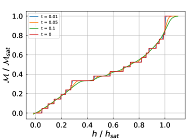
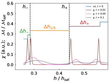
Figure 1: (Color online) Magnetization curves of the kagomé lattice with $N=42$ sites (top) as well as with $N=48$ sites (bottom) for various temperatures together with the differential susceptibility for $N=48$ (bottom). The asymmetric melting of the plateau at $\nicefrac{{1}}{{3}}$ of the saturation magnetization is clearly visible, compare also [43]. $h_{-}$ and $h_{+}$ define the end points of the $\nicefrac{{1}}{{3}}$-plateau; $\Delta h_{1/3}$ denotes its width, whereas $\Delta h_{-}$ and $\Delta h_{+}$ are the widths of the neighboring magnetization steps.

Magnetization curve:

The afore-mentioned asymmetric melting of the $\nicefrac{{1}}{{3}}$-plateau can be quantified by comparing the thermal behavior at the low-field end $h_{-}$ and at the high-field end $h_{+}$ of the plateau, see Fig. 1. One can see that for increasing temperatures the magnetization at $h_{-}$ drops rapidly from the zero-temperature value of $\nicefrac{{1}}{{3}}$ whereas the value of magnetization at $h_{+}$ roughly stays the same even for higher temperatures. A suggested explanation of this asymmetric phenomenon is that the density of states at low energies of the $M_{1/3}$-subspace is far denser than that of the $M_{1/3}+1$-subspace and that the density of states of the $M_{1/3}-1$-subspace must be even denser [43, 44].

As discussed in recent articles [43, 44] and shown later on, this explanation is partially correct, but there is an additional cause for this phenomenon to be mentioned. As can be seen in Fig. 1, the ($\nicefrac{{1}}{{3}}{-1}$)-step is very small, especially compared to the ($\nicefrac{{1}}{{3}}{+1}$)-step. This suggests that for low temperatures where at $h_{+}$ only states from two subspaces contribute significantly to the magnetization, at $h_{-}$, states from three or four subspaces are involved. In Ref. MMY:PRB20, the possible influence of additional subspaces is acknowledged but not further investigated.

Figure 2 demonstrates that the step size $\Delta h_{+}$ is (typically much) greater than $\Delta h_{-}$ for all investigated system sizes. Even though the details vary due to finite size effects it is evident that the width $\Delta h_{-}$ of the low-field step is typically significantly less than a fifth of the width $\Delta h_{+}$ of the high-field magnetization step, compare r.h.s. of Fig. 2. The differences between $N=45$ and $N=42,48$ in Fig. 2 could be related to the nature of the $\nicefrac{{1}}{{3}}$-plateau state that can be understood as a valence-bond state with a magnetic unit cell of 9 spins [30, 33, 34, 24] and therefore fits much better to $N=45$ than to $N=42$ or $48$.

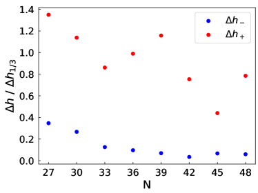
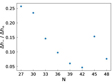
Figure 2: (Color online) The widths of the ($\nicefrac{{1}}{{3}}{-1}$)-step $\Delta h_{-}$ and of the ($\nicefrac{{1}}{{3}}{+1}$)-step $\Delta h_{+}$, respectively. Top: normalized values, bottom: ratio $\Delta h_{-}/\Delta h_{+}$.

In order to investigate which subspaces $\mathcal{H}_{M}$ contribute dominantly to the magnetization at low temperatures, we compare the deviations from the exact value when estimating the magnetization with only subsets of the subspaces $\mathcal{H}_{M}$. To this end we define the following subsets:

$$\Gamma_{2} \left(h_{-}\right):=\{M_{1/3},M_{1/3}-1\}$$ (6)

$$\Gamma_{3} \left(h_{-}\right):=\{M_{1/3},M_{1/3}-1,M_{1/3}-2\}$$ (7)

to be used for $\mathcal{M}(T,h_{-})$. Here $\Gamma_{2}\left(h_{-}\right)\subset\Gamma_{3}\left(h_{-}\right)$, i.e., $\Gamma_{2}\left(h_{-}\right)$ yields a more restrictive approximation of the magnetization.

To determine similar deviations at $h_{+}$ we consider the subsets

$$\Gamma_{2} \left(h_{+}\right):=\{M_{1/3}+1,M_{1/3}\}$$ (8)

$$\Gamma_{3} \left(h_{+}\right):=\{M_{1/3}+2,M_{1/3}+1,M_{1/3}\}\ ,$$ (9)

where $\Gamma_{2}\left(h_{+}\right)\subset\Gamma_{3}\left(h_{+}\right)$. The subspace associated with these sets is defined as

$$\mathcal{H}(\Gamma_{k}(h)):=\bigoplus_{M\in\Gamma_{k}(h)}\mathcal{H}_{M}\ .$$ (10)

The sets $\Gamma_{k}(h)$ are chosen such that $\mathcal{H}(\Gamma_{k}(h))$ contains the $k$ lowest-lying subspaces for the applied magnetic field $h$. We define the deviation

$$\Delta\mathcal{M}_{\Gamma_{i}}(T,h)=\big{|}\mathcal{M}(T,h)-\mathcal{M}_{\Gamma_{i}}(T,h)\big{|}\ ,$$ (11)

where $\mathcal{M}_{\Gamma_{i}}(T,h)$ denotes the approximation of the magnetization using only the subspace $\mathcal{H}(\Gamma_{i}(h))$ .

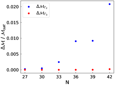
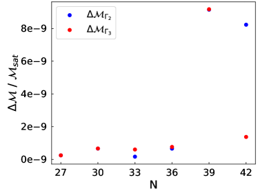
Figure 3: (Color online) Normalized deviations $\Delta\mathcal{M}_{\Gamma_{i}}(t,h)$ at $t=0.05$, compare (11), for various system sizes. The deviations at $h_{-}$ (top) are six orders of magnitude bigger than for $h=h_{+}$ (bottom), see text.

As can be seen in Fig. 3 (top), the deviations for $h=h_{-}$ are of the order of $\nicefrac{{1}}{{100}}$ of the saturation magnetization, when only considering subspace $\mathcal{H}(\Gamma_{2}(h_{-}))$. When using the greater subspace $\mathcal{H}(\Gamma_{3}(h_{-}))$ the deviations are significantly lower ($\leq 1$ ‰). This means, that even at temperatures as low as $t=0.05$ there are more than just two subspaces $\mathcal{H}_{M}$ significantly contributing to the value of $\mathcal{M}(T,h)$ at the magnetization jump to the ($\nicefrac{{1}}{{3}}{}$)-step, i.e. at $h=h_{-}$ .

In Fig. 3 (bottom), the deviations for $h=h_{+}$ are of the order of $\sim 10^{-9}$, i.e. six orders of magnitude smaller, even when only regarding the subspace $\mathcal{H}(\Gamma_{2}(h_{+}))$ which consists of only two subspaces $\mathcal{H}_{M}$. To achieve the same accuracy at $h=h_{-}$ one would have to consider at least four subspaces $\mathcal{H}_{M}$.

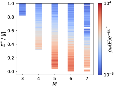
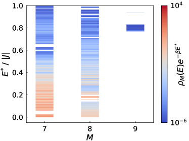
Figure 4: (Color online) Low-energy part of the subspace densities of states $\rho_{M}(E^{*})$ of the energetically lowest subspaces for $E^{*}=(E-E_{0}(M))/|J|\leq 20\cdot t$) weighted by the Boltzmann factor at $t=0.05$ and calculated at $h_{-}$ (top) and $h_{+}$ (bottom) for the KHAF with $N=42$ sites. Values smaller than $10^{-7}$ are omitted to improve resolution of the color coding.

Density of states:

Next, we consider subspace densities of states $\rho_{M}(E,h)$ at $h_{-}$ and $h_{+}$ for $N=42$ sites to get an even more profound understanding of the melting process. Therefore, we show in Fig. 4 the low-energy part of the densities of states of the energetically lowest subspaces weighted by the Boltzmann factor at $t=0.05$. Values smaller than $10^{-7}$ are omitted to improve the resolution of the color coding, which yields the white spaces in Fig. 4 although the density of states is not strictly zero.

As can be seen in Fig. 4 (top) the density of low-lying levels is indeed larger in the subspace with $M_{1/3}-1$ than in the plateau subspace with $M_{1/3}$, and this density is larger than that of the subspace with $M_{1/3}+1$, as was conjectured previously [43, 44]. In addition, two subspaces with $M_{1/3}-1$ and $M_{1/3}-2$ contribute to thermal expectation values at small excitation energies at the low-field side of the plateau whereas only one subspace with $M_{1/3}+1$ contributes at the high-field side of the plateau.

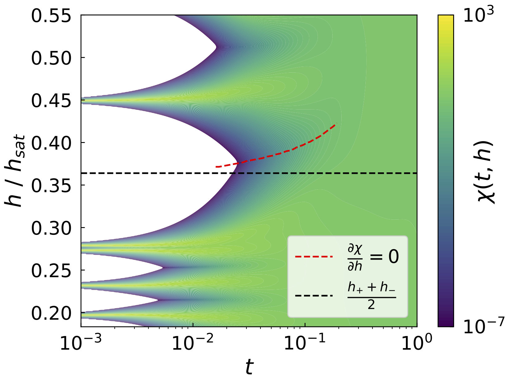
Figure 5: (Color online) The differential magnetic susceptibility $\chi(t,h)$ for the KHAF with $N=42$ sites. Values smaller than $10^{-8}$ are omitted to improve resolution of the color coding. The asymmetric melting of the $\nicefrac{{1}}{{3}}$-plateau is visible as an upturn of the region of small susceptibility around $h\sim 0.28\dots 0.45$. It is additionally highlighted by the red dashed curve (local minimum of $\chi(t,h)$) that deviates clearly from the symmetric black dashed line.

Finally, we graphically summarize the melting of magnetization plateaus by plotting the differential magnetic susceptibility $\chi(t,h)$ for the KHAF with $N=42$ sites in Fig. 5. A flat magnetization plateau corresponds to zero susceptibility, melting increases the susceptibility, and an asymmetric increase expresses itself as a banana-shaped feature. This behavior is clearly visible in Fig. 5 in the region around $h\sim 0.28\dots 0.45$ and additionally highlighted by the red dashed curve (local minimum of $\chi(t,h)$) bending towards higher fields compared to a symmetric behavior shown by the black dashed curve.

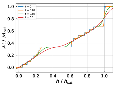
Figure 6: (Color online) Magnetization curve of the square-kagomé lattice with $N=42$ sites at low temperatures in comparison to the zero temperature curve. The $\nicefrac{{1}}{{3}}$-plateau melts symmetrically.

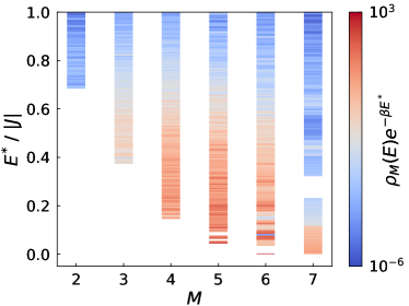
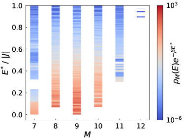
Figure 7: (Color online) Low-energy part of the subspace densities of states $\rho_{M}(E)$ of the energetically lowest subspaces for $E_{0}(M)/|J|\leq 20\cdot t$) weighted by the Boltzmann factor at $t=0.05$ and calculated at $h_{-}$ (top) and $h_{+}$ (bottom) for the SKHAF with $N=42$ sites. Values smaller than $10^{-7}$ are omitted to improve resolution of the color coding.

3.2 No asymmetric melting of the SKAHF $\nicefrac{{1}}{{3}}$-plateau

As a counter example we will consider the melting of the $\nicefrac{{1}}{{3}}$-plateau of the square-kagomé lattice antiferromagnet (SKHAF). In Fig. 6 one can see that the plateau melts symmetrically with increasing temperatures.

Comparing Fig. 6 of the SKHAF with Fig. 1 of the KHAF one notices that for the SKHAF the magnetization steps to either side of the $\nicefrac{{1}}{{3}}$-plateau have very similar sizes in contrast to our findings for the KHAF.

Looking at the densities of low-lying states of the subspaces with $M_{1/3}-1$, $M_{1/3}$, and $M_{1/3}+1$ we find a different trend for the SKHAF compared to the KHAF: the density does not steadily increase with increasing $M$, it is largest for $M_{1/3}$ and decreases when going to either $M_{1/3}-1$ or $M_{1/3}+1$, see Fig. 7. This means roughly that at both edges of the plateau a similar number of subspaces contributes significantly to the value of the magnetization. One should keep in mind, that these contributions consist of the density of states multiplied by the Boltzmann factor as well as the magnetic quantum numbers, and that the symmetry we discuss is visible only at rather small temperatures, i.e., for Boltzmann factors that decrease rapidly with increasing energy.

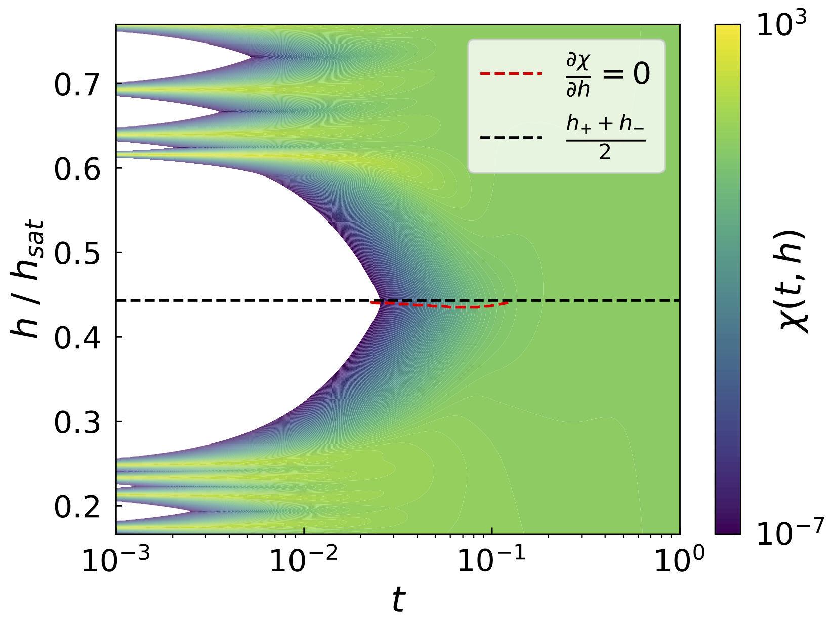
Figure 8: (Color online) The magnetic susceptibility $\chi(h,t)$ for $42$ sites on the square-kagomé lattice. Values smaller than $10^{-8}$ are dropped to improve resolution of the color coding. The symmetric melting of the $\nicefrac{{1}}{{3}}$-plateau is clearly visible around $h\sim 0.27\dots 0.61$. It is additionally highlighted by the red dashed curve that does not deviate from the symmetric black dashed line.

We again graphically summarize the melting of magnetization plateaus by plotting the differential magnetic susceptibility $\chi(t,h)$ for the SKHAF with $N=42$ sites in Fig. 8. The figure clearly demonstrates that the $\nicefrac{{1}}{{3}}$-plateau melts symmetrically, see region around $h\sim 0.27\dots 0.61$ in Fig. 8. The dashed red curve which marks the minimum of the susceptibility does not deviate from the symmetric black dashed line.

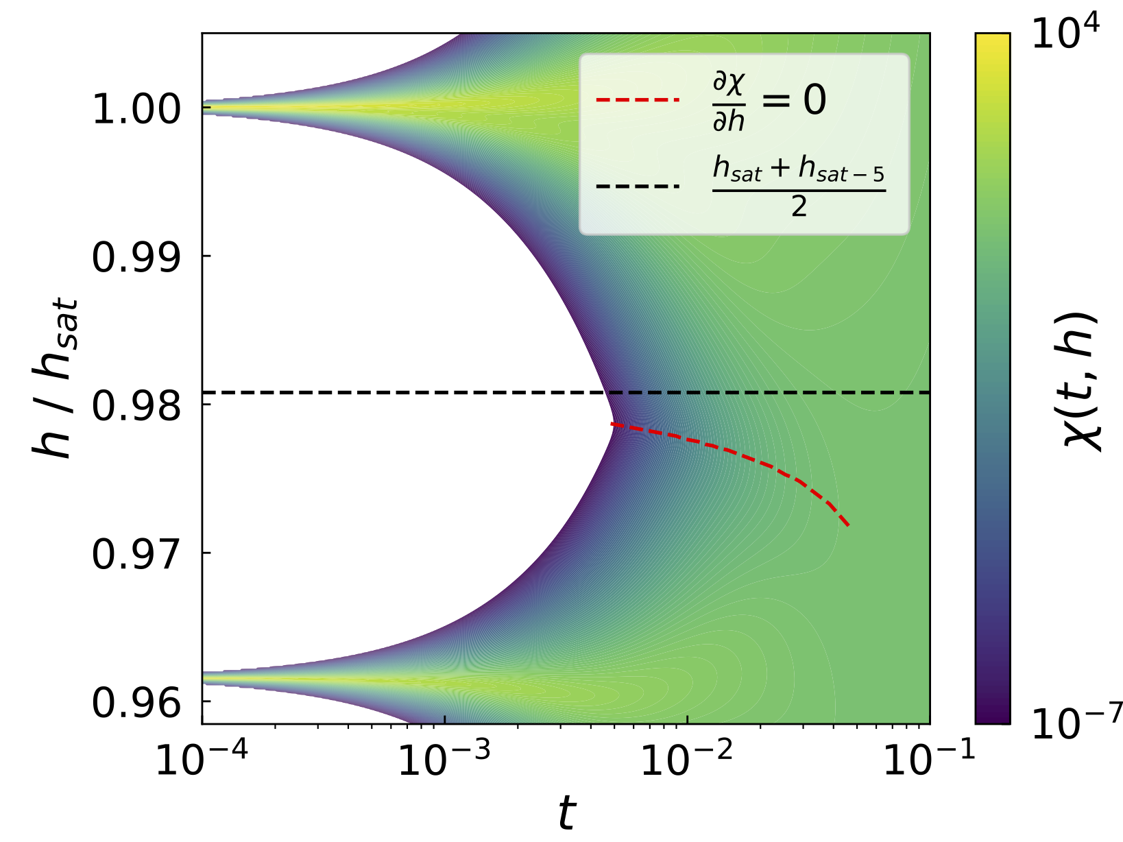
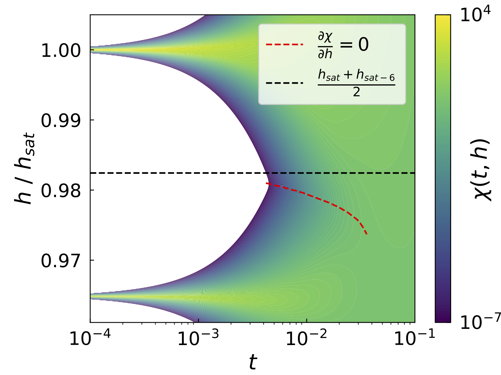
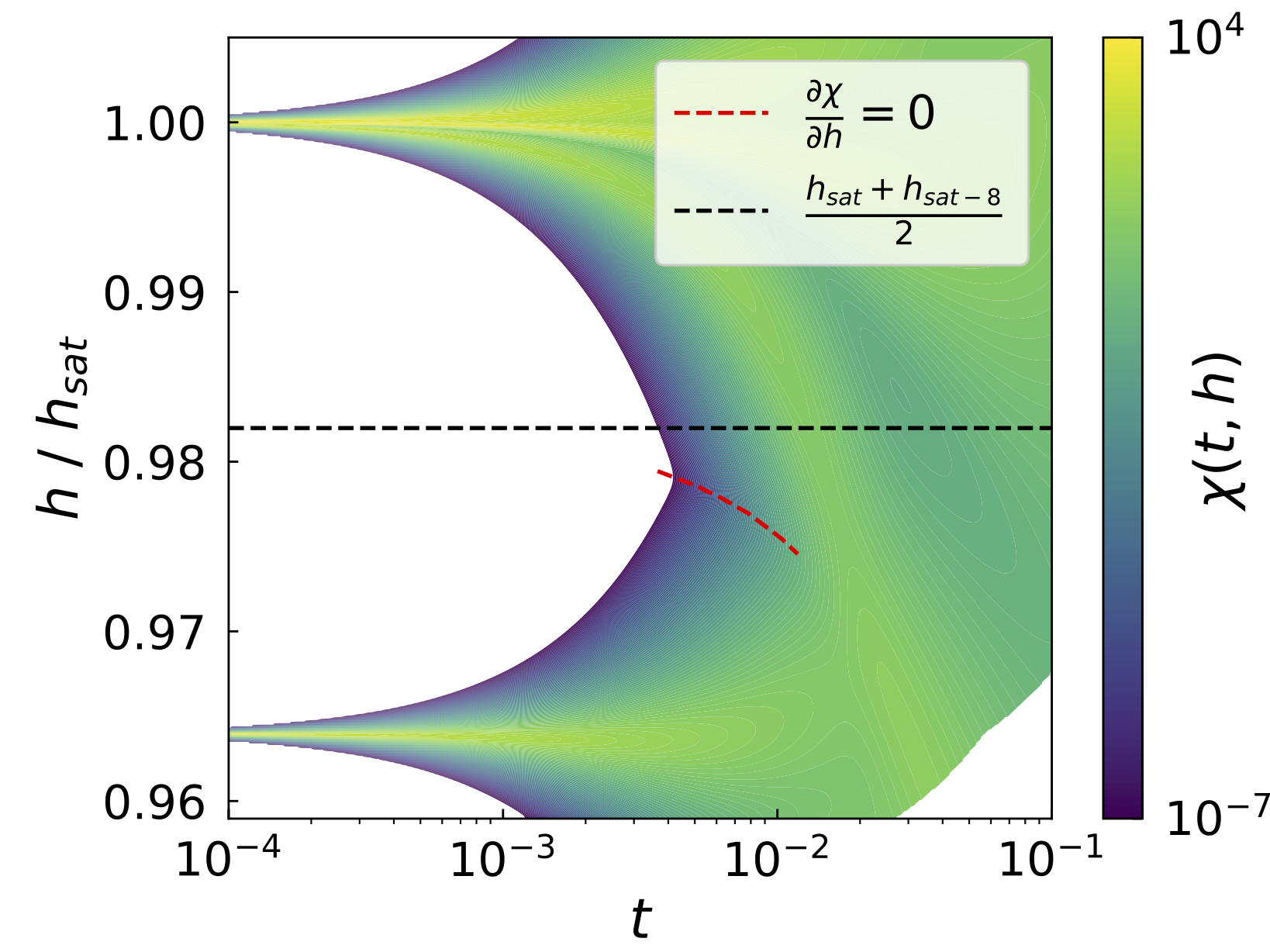
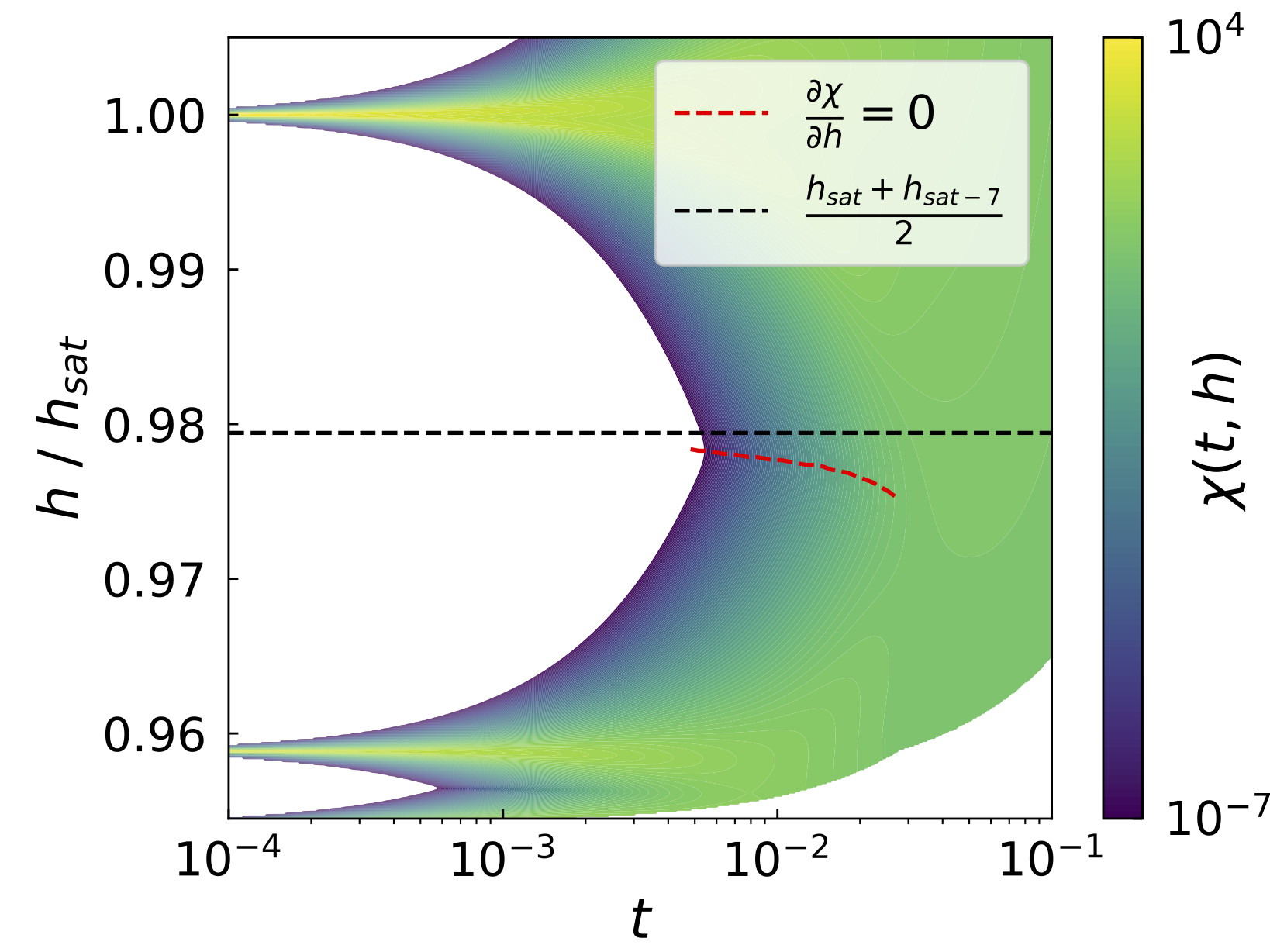
Figure 9: (Color online) Magnetic susceptibility $\chi(h,t)$ for the KHAF of $N=45,54,63,72$ sites (clockwise from top left). Values smaller than $10^{-8}$ are dropped to improve the resolution of the color coding. The $\nicefrac{{7}}{{9}}$-plateau melts asymmetrically with a downturn of the minimum of the susceptibility, see red dashed curves.

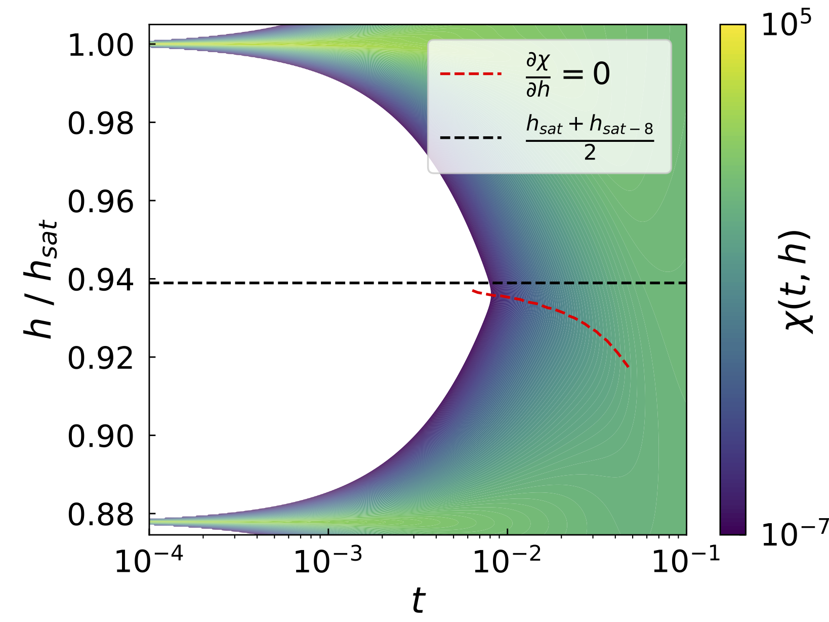
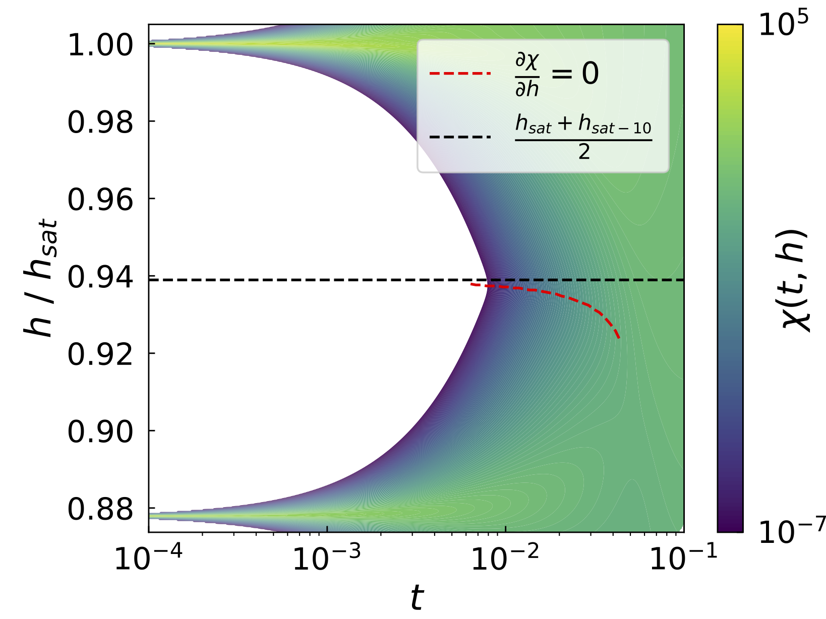
Figure 10: (Color online) Magnetic susceptibility $\chi(h,t)$ for the SKHAF of $N=42,48,54,60$ sites (clockwise from top left). Values smaller than $10^{-8}$ are dropped to improve the resolution of the color coding. The $\nicefrac{{2}}{{3}}$-plateau melts asymmetrically with a downturn of the minimum of the susceptibility, see red dashed curves.

3.3 Excursus – plateau next to saturation

Although the $\nicefrac{{1}}{{3}}$-plateau melts differently for the KHAF and the SKHAF the magnetization plateau that precedes the magnetization jump to saturation, compare [26, 43, 59], melts asymmetrically for both lattices as depicted by the dashed red curves of minimal susceptibility in Figs. 9 and 10. In contrast to the asymmetric melting of the $\nicefrac{{1}}{{3}}$-plateau of the KHAF here we observe a pronounced bending towards lower fields. This feature is related to the very existence of a flat one-magnon band [62, 63] and is therefore a generic effect of flat-band quantum magnets. For spin systems with a flat one-magnon band the structure of the density of low-lying states at and below the saturation field is very similar and dominated by localized multi-magnon states that are degenerate at the saturation field and split up for smaller fields as well as by the nearly exponentially growing dimension of subspaces $\mathcal{H}_{M}$ with decreasing $|M|$. Therefore, we may expect that the asymmetric melting of this high-field plateau is present also if the flat-band becomes slightly dispersive, as for example in the diamond-shaped compound azurite [64, 65, 66].

A possible difference between various flat-band systems could be given by the magnetization of the plateau that precedes the magnetization jump to saturation. For the KHAF this is $\nicefrac{{7}}{{9}}$ and for the SKHAF this is $\nicefrac{{2}}{{3}}$ of the saturation magnetization, respectively [26, 43, 59]. Figure 9 shows the magnetic susceptibility of the KHAF for fields close to saturation and temperatures $t=10^{-4},\dots 10^{-1}$ for $N=45,54,63,72$ sites (clockwise from top left). Figure 10 displays the magnetic susceptibility of the SKHAF for fields close to saturation and temperatures $t=10^{-4},\dots 10^{-1}$ for $N=42,48,54,60$ sites (clockwise from top left). Here $h_{\text{sat}}$ denotes the saturation field, and $h_{\text{sat}-k}$ denotes the low-field end of the plateau, where $k$ is the largest number of localized multi-magnon states that fits on the respective size of the lattice.

All cases clearly exhibit asymmetric melting towards lower fields for increasing temperatures.

4 Discussion and conclusions

The experimental magnetization is often not directly determined but via its derivative with respect to the applied field, i.e., the susceptibility, in particular for instance in pulsed field measurements, see, e.g. [65, 67, 68] for recent related examples. Therefore, the question how plateaus deform with elevated temperatures is very relevant for the interpretation of measurements of the magnetization. Asymmetric melting means that the minimum of the susceptibility moves away from the center of the $(T=0)$-plateau with rising temperature.

Looking at our findings, we tend to conclude that the main cause of the asymmetric melting of the $\nicefrac{{1}}{{3}}$-plateau of the KHAF is that only two subspaces contribute to the magnetization at the right edge of the $\nicefrac{{1}}{{3}}$-plateau at low temperatures whereas at the left edge several subspaces with a broader spread of magnetic quantum numbers contribute for the same temperature. In the case of the SKHAF the latter is the case at both ends of the plateau which results in a more symmetric melting.

Appendix A Constructing a density of states

Through a suitable shift of the energy scale ($E_{0}>0)$ the partition function can be written as the Laplace transform of the density of states:

$$Z(\beta)=\int_{0}^{\infty}\rho(E)e^{-\beta E}\text{d}E\quad$$ (12)

with

$$\rho(E)=\sum_{n}\delta(E-E_{n})$$ (13)

Hence an inverse Laplace transformation of the partition function approximated by FTLM will give an approximation of the density of states:

$$\rho_{\text{FTLM}}=\frac{1}{2\pi\textbf{i}}\int_{c-\textbf{i}\infty}^{c+\textbf{i}\infty}Z_{\text{FTLM}}(\beta)e^{\beta E}\text{d}\beta\ .$$ (14)

By substituting $\beta$ with $c+\textbf{i}s$ one finds:

$$\rho_{\text{FTLM}}(E)=\frac{\textbf{i}}{2\pi\textbf{i}}\int_{-\infty}^{\infty}Z_{\text{\scriptsize FTLM}}(c+\textbf{i}s)e^{(c+\textbf{i}s)E}\text{d}s$$ (15)

$$=\frac{1}{2\pi}\sum_{\Gamma,n,r}\gamma_{n}^{(r,\Gamma)}\int_{-\infty}^{\infty}e^{-(c+\textbf{i}s)\epsilon^{(r,\Gamma)}_{n}}e^{(c+\textbf{i}s)E}\text{d}s$$ (16)

$$=\sum_{\Gamma,n,r}\gamma_{n}^{(r,\Gamma)}e^{-c(\epsilon^{(r,\Gamma)}_{n}-E)}\frac{1}{2\pi}\int_{-\infty}^{\infty}e^{-\textbf{i}s(\epsilon^{(r,\Gamma)}_{n}-E)}\text{d}s$$ (17)

$$=\sum_{\Gamma,n,r}\gamma_{n}^{(r,\Gamma)}\delta(\epsilon^{(r,\Gamma)}_{n}-E)\ .$$ (18)

The difficulty is now to find a suitable representation of the $\delta$-distribution, which will give a good representation of the density of states as well. For (energetically) bounded systems a rectangular function

$$\delta_{\varepsilon}(x)=\begin{cases}\frac{1}{\varepsilon}&\ \text{if}\ |x|\leq\frac{\varepsilon}{2}\\ 0&\ \text{else}\end{cases}$$ (19)

is convenient because it is also a bounded function and therefore will not give non-zero values outside the true spectrum. An additional problem of the representation is that the number of pseudo-eigenvalues obtained from the FTLM approximation is much smaller than the dimension of the Hilbert space. So if $\varepsilon$ is chosen too small it is possible to produce gaps where in the exact density of states there are no gaps. This issue is of course only relevant in very dense parts of the density. As a solution one can choose the bounds of the rectangular functions to always be the mean of to consecutive pseudo-eigenvalues so that all gaps will be closed [69]. For this one defines an asymmetric version of the rectangular function:

$$\delta_{\varepsilon,\,\varepsilon^{\prime}}(x)=\begin{cases}\frac{1}{\varepsilon+\varepsilon^{\prime}}&\ \text{if}\ -\varepsilon^{\prime}\leq x\leq\varepsilon\\ 0&\ \text{else}\end{cases}\ .$$ (20)

the parameters will chosen such that the bounds will lie at mean of to consecutive but non-degenerate pseudo-eigenvalues. Let $\epsilon_{k}^{\Gamma}$ be the sorted but pairwise distinct pseudo-eigenvalues of a subspace $\Gamma$, then the $\delta$-distributions can be replaced by

$$\delta(\epsilon^{\Gamma}_{k}-E)\rightarrow\delta_{\varepsilon_{+},\,\varepsilon_{-}}(\epsilon^{\Gamma}_{k}-E)\quad$$ (21)

with

$$\varepsilon_{-}=\tfrac{\epsilon^{\Gamma}_{k}-\epsilon^{\Gamma}_{k-1}}{2},\ \varepsilon_{+}=\tfrac{\epsilon^{\Gamma}_{k+1}-\epsilon^{\Gamma}_{k}}{2}\ .$$ (22)

Lanczos weights of (numerically) degenerate pseudo-eigenvalues will be binned and added, where $N_{\text{\scriptsize dis}}$ denotes the number of pseudo-eigenvalues without the dropped duplicates. This gives rise to the following representation of the density of states:

$$\rho_{\text{FTLM}}(E)\approx\sum_{\Gamma}\sum^{N_{\text{\scriptsize dis}}}_{k=1}\gamma_{k}^{\Gamma}\delta_{\varepsilon_{+},\,\varepsilon_{-}}(\epsilon^{\Gamma}_{k}-E)\ .$$ (23)