Detached eclipsing binaries from the Kepler field: radii and photometric masses of components in short-period systems

Abstract

The characterisation of detached eclipsing binaries with low mass components has become important when verifying the role of convection in stellar evolutionary models, which requires model-independent measurements of stellar parameters with great precision. However, spectroscopic characterisation depends on single-target radial velocity observations and only a few tens of well-studied low-mass systems have been diagnosed in this way. We characterise eclipsing detached systems from the Kepler field with low mass components by adopting a purely-photometric method. Based on an extensive multi-colour dataset, we derive effective temperatures and photometric masses of individual components using clustering techniques. We also estimate the stellar radii from additional modelling of the available Kepler light curves. Our measurements confirm the presence of an inflation trend in the mass-radius diagram against theoretical stellar models in the low-mass regime.

1 Introduction

The characterisation of eclipsing binaries (EBs), especially detached systems with low mass components (with $M_{\star}\leq 0.7M_{\odot}$), has become a good approach for testing stellar evolutionary models, concerning the role of convection in these later type stars (Feiden & Chaboyer, 2012; Han et al., 2019). This requires unbiased, high-precision measurements of stellar masses and radii in large homogeneous samples. By combining spectroscopic and photometric time-series data, it is possible to determine the physical properties (radii and masses) of EB components with uncertainties of $5\%$ or less (e.g. Torres & Ribas, 2002; López-Morales & Ribas, 2005; Birkby et al., 2012). Such well characterised detached systems in very close orbits – with orbital periods ($P_{\rm orb}$) of 2-3 days or less – show discrepancies when compared to stellar models: the estimated radii can be $5$-to-$20\%$ larger than predicted (López-Morales & Ribas, 2005; Kraus et al., 2011; Cruz et al., 2018; Chaturvedi et al., 2018). However, just a few tens of well-charaterised detached EB (DEB) systems are available in the literature (Southworth, 2015; Chaturvedi et al., 2018).

In order to explain the measured anomalous radius of low-mass stars, several scenarios were proposed in the past years and remain discussed to date in the literature. For example, López-Morales (2007) proposed that the stellar metallicity would play a role, as it was observed that isolated metal-rich stars presented larger radii than expected. The magnetic activity was also pointed as responsible, where M-dwarf stars in detached short-period systems would have an enhanced activity, which would inhibit convection and cause their radius to inflate (Chabrier et al., 2007; Kraus et al., 2011). Moreover, part of the radius anomaly problem could come from the current stellar models, which are not able to fully reproduce the properties of active low-mass star (Morales et al., 2010; Irwin et al., 2011).

It is important to increase the sample of known low-mass DEBs to investigate the radius anomaly causes. Nevertheless, the proper spectroscopic characterisation is time-consuming and depends on a lot of telescope time. Garrido et al. (2019) have then adopted a purely-photometric method to characterise $230$ short-period DEBs from the Catalina Sky Survey (CSS Drake et al., 2009), with $P_{\rm orb}<2$ days, using available broad-band photometric data and CSS light curves (LCs) only. The mentioned method provided the fractional radius of each component, estimated from light-curve modeling. They also derived photometric masses, which were obtained based on a multi-color dataset by using clustering techniques, as a confirmation of the low-mass nature of the binary components (for more details, see Garrido et al., 2019). Regardless large individual uncertainties, their work have considerably increased the number of known systems with main-sequence low-mass components.

The use of machine learning algorithms has become more frequent and has been adopted for data mining and automated classification in astronomical databases (Sánchez Almeida & Allende Prieto, 2013; Chattopadhyay & Chattopadhyay, 2014, and references therein). In this work, we aim to identify new DEB systems with low mass components. For that, we adopted unsupervised and supervised methods to classify previously identified binary systems from the Kepler space mission (Borucki et al., 2010) according to their luminosity class, using a multi-colour dataset, and derive the effective temperature and the photometric mass of each individual component by searching for similarities between observed data and models, as done in Garrido et al. (2019). Moreover, we used the available Kepler LCs to derive the fractional radius and orbital parameters of selected EB systems.

This paper is organised as follows. The sample selection is described in Sect. 2. The characterisation of each binary component individually is presented in Sect. 3, which includes the description of the adopted machine learning methods. The analysis is presented in Sect. 4, which shows the adopted LC modelling procedure and the obtained results. In Sect. 5, we present the comparison with previous works and a discussion on the obtained mass-radius diagram, and finally in Sect. 6, our conclusions.

2 Sample Selection

We selected eclipsing binary systems from the Kepler Eclipsing Binary Catalog (Third Revision, Kirk et al., 2016, hereafter KEBC), with orbital period of $4$ days or less, and with effective temperature ($T_{\rm eff}$) up to $6\,000$K. Note that $T_{\rm eff}$ available at the catalogue was derived by the authors from the stellar energy distribution (SED), based on broad-band photometry and assuming a single star configuration (for details, see Kirk et al., 2016). Therefore, these temperatures were used only as a selection criterion.

The selection was cross-matched to broad-band photometric catalogs, keeping only those EB systems with available data from the Panoramic Survey Telescope and Rapid Response System (Pan-STARRS; Tonry et al., 2012) and Two-Micron All-Sky Survey (2MASS; Skrutskie et al., 2006). Only those with data in all offered filters – $g\,r\,i\,z\,y$ from Pan-STARRS and $J\,H\,K_{\rm s}$ from 2MASS – were kept. Differently from our previous work (Garrido et al., 2019), we used the Pan-STARRS photometry to cover the region of the visible because the Sloan Digital Sky Survey (SDSS; Abazajian et al., 2009) is not available for the whole Kepler field. Finally, we also excluded those systems that presented any warning flag in the available broad-band photometry, indicating possible spurious measurements. We selected, then, a list of $821$ EB systems to undergo a light curve (LC) inspection.

2.1 Light curves

The light curves were obtained from Kepler’s database, where we downloaded the long-cadence data from all observed quarters for each selected EB. To obtain normalized LCs, we adopted the sliding median method, dealing with each available quarter of observations separately for each object individually. A median LC is generated by sliding a window with a fixed size (in number of epochs) along the light curve and replacing the central point by the calculated median within the window. The size of the window is different for each quarter and each object, as it is calculated as being the one with the highest chi-square when both LCs are compared, the original and the generated median LC, after iteration using different window sizes. The median LC was then fitted by a cubic spline function to obtain a more smooth normalization curve, which was used to correct the original light curve. Figure 1 shows the results of such normalization procedure for KIC09656543 as an example. Top and middle panels show the calculated median light curve in green, resulting from the sliding median window, and the red curve represents the normalization function obtained by the spline fit. The normalized light curve (for tenth quarter) is presented on the bottom panel. Repeating the same procedure with all available quarters for a given EB, we obtained the complete normalized light curve.

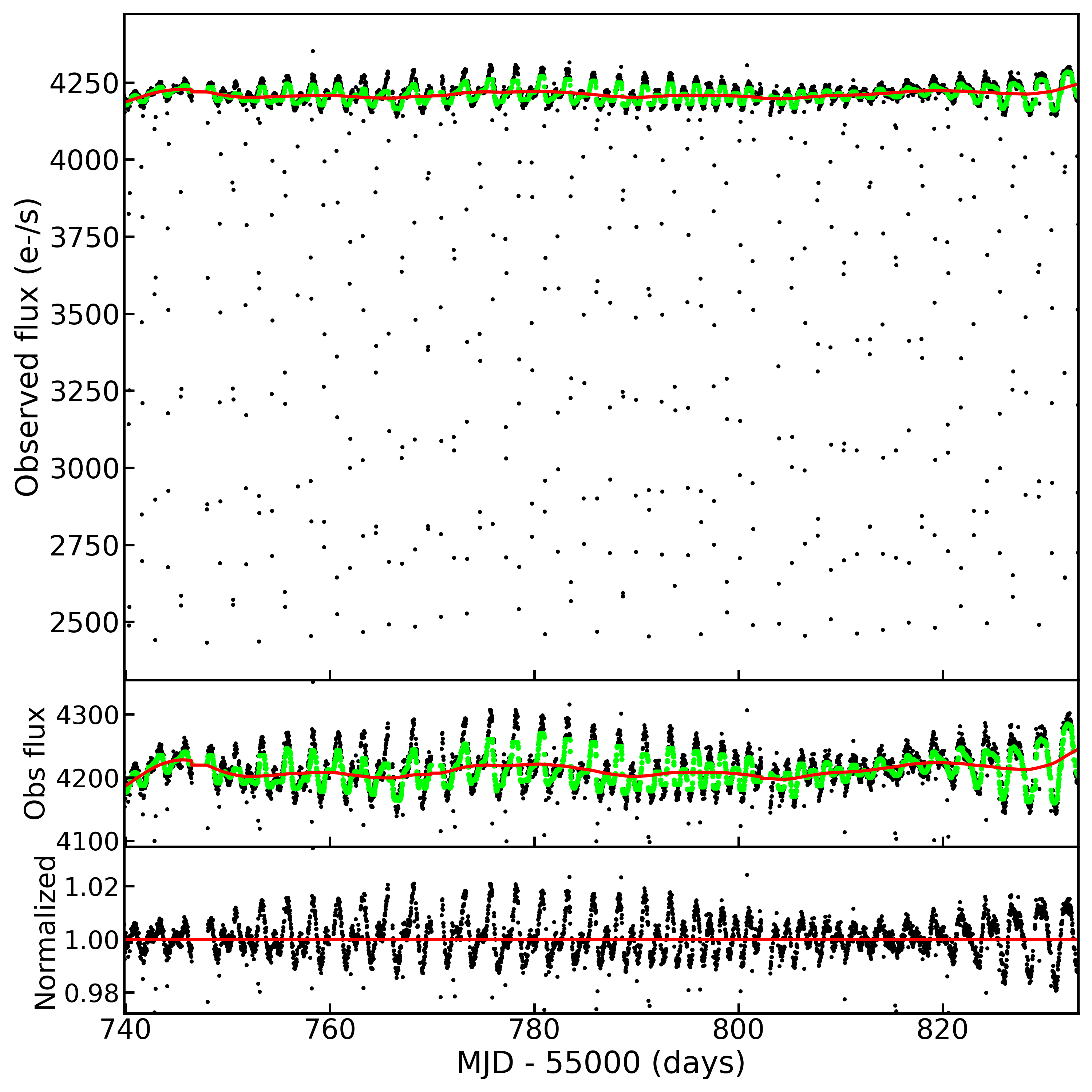
Figure 1: Normalization of the tenth quarter of observations for EB KIC09656543. Top panel: The black dots show Kepler light curve, with 4179 epochs. The green curve is the calculated median curve, and the red line shows the spline fit. Middle panel: The same as previous plot, but zoomed in the LC baseline. Bottom panel: The obtained light curve, showing the resulting normalization along the baseline.

2.2 Sample of detached binaries

Matijevič et al. (2012) adopted an automatic procedure, the Locally Linear Embedding (LLE) method, to derive the morphological class of eclipsing binaries – distinguishing between detached, semi-detached, and contact systems – which is presented as a morphology value, c, in the KEBC catalogue (Kirk et al., 2016). According to Matijevič et al. (2012), if the classification parameter $c$ is less than $0.5$, a system is probably a detached system. If $c$ lays between $0.5$ and $0.7$, a system is more likely to be a semi-detached binary and the contact systems may have $c$ between $0.7$ and $0.8$. These authors mentioned that well-detached system should have $c<0.1$ and almost sinusoidal LCs should have $c>0.9$. They also stated that the derived morphology value presented in the catalog should be taken only as a guideline, as the separation between different classes is not abrupt. For instance, there are detached systems with estimated $c\sim 0.7$, and semi-detached ones with $c\sim 0.4$ (for example, see Matijevič et al., 2012, Fig. 4).

Therefore, all light curves underwent an independent visual inspection to separate them into the three morphological classes. For that, we generated the phase-folded curves by adopting the binary orbital period given in the KEBC catalog (Kirk et al., 2016). Some of the LCs presented intense baseline variation – what could due to a strong stellar activity or other unidentified cause that turned the visual classification ambiguous – and, therefore, they were excluded. From the $821$ LCs inspected (the selected objects described previously in this section), $300$ of them could be classified as detached EB systems (DEBs). As a comparison to the results obtained from the LLE method, which are available at the KEBC catalog, $60$% of our DEB sample have $c<0.5$ and $48$% of them have $0.5<c<0.7$.

3 Characterisation of binary components

We constructed a ten-colour grid of models with synthetic composite colours – based on the available broad-band photometric data from Pan-STARRS ($g\,r\,i\,z\,y$) and 2MASS ($J\,H\,K_{\rm s}$) – to identify the EB systems with only main-sequence stars as components. We adopted colour indices to discriminate dwarf stars from systems with evolved components. For that, we used models for giant stars to represent and discriminate from possible evolved stars – like subgiants, for instance – as their spectral energy distribution – and, therefore, their colours – resemble those of giant stars.

This calibration grid was generated based on evolutionary models with $1$, $3$, and $5$ Gyr from Bressan et al. (2012), considering three possible EB configurations: systems composed by two dwarf stars (V+V), by a dwarf and a giant (V+III), and by two giants (III+III), where giant models represent evolved components. We used a total of $1\,020$ different models: $903$ models for giant stars, with $T_{\rm eff}$ from $1\,624$ to $5\,979$ K, and $117$ for dwarfs, with $T_{\rm eff}$ from $2\,303$ to $5\,991$ K. These models were combined two-by-two to generate synthetic model binaries, as done by Parihar et al. (2009), which resulted in a detailed synthetic grid with $180\,579$ different binary models.

For the PanSTARRS-2MASS ten-colour model grid, we adopted the seven standard colours with adjacent passbands – $(g-r)$, $(r-i)$, $(i-z)$, $(z-y)$, $(y-J)$, $(J-H)$, $(H-K_{\rm s})$ – added to the same three redder colours adopted by Garrido et al. (2019) to better identify the V+V binaries – $(r-J)$, $(r-H)$ and $(z-K_{\rm s})$.

3.1 Defining temperatures using machine learning algorithms

We searched for similarities between the observed photometry and models to classify our DEB sample according to their luminosity class, and derive the effective temperature of each individual component. For that, we followed the same methodology described in Garrido et al. (2019), which is briefly described below.

We adopted the $k$-means clustering technique, starting with the Hartigan test (Hartigan, 1975), which was applied to the calibration grid with over $180\,000$ synthetic binaries jointly with the $821$ selected EBs (see Sect. 2), aiming at optimising the number of clusters that should be formed. The Hartigan test reached the optimal solution of $17$ clusters after 50 iterations. We then performed the $k$-means method to assign the data to each cluster, by distributing the whole dataset (models and observed data) into $17$ separate clusters. The cluster centroids are initially randomly defined, and then recalculated over several iterations until they reach convergence, where distances between the centroid and the data are minimal.

Table 1: Effective temperatures and photometric masses obtained for a test set of well known V+V binaries, with available Pan-STARRS and 2MASS photometry. The estimated $T_{\rm eff}$ and $M_{\star}$ values are shown in columns 2-5 and the comparison values (from literature) are presented in columns 6-9. The respective references are presented in the last column.

Star Name	$\mathrm{T}_{1}$ (K)	$\mathrm{T}_{2}$ (K)	$\mathrm{M}_{1}$ (M⊙)	$\mathrm{M}_{2}$ (M⊙)	$\mathrm{T}_{1,pub}$ (K)	$\mathrm{T}_{2,pub}$ (K)	$\mathrm{M}_{1,pub}$ (M⊙)	$\mathrm{M}_{2,pub}$ (M⊙)	Reference
	(K)	(K)	(M⊙)	(M⊙)	(K)	(K)	(M⊙)	(M⊙)
Correctly assigned V+V systems
2MASS J01542930+0053266	3698$\pm$100	2742$\pm$552	0.504$\pm$0.032	0.091$\pm$0.186	3800	3600	0.515$\pm$0.023	0.548$\pm$0.025	Becker et al. (2008)
2MASS J10305521+0334265	3700$\pm$100	3054$\pm$430	0.505$\pm$0.032	0.161$\pm$0.229	3720$\pm$20	3630$\pm$20	0.499$\pm$0.002	0.444$\pm$0.002	Kraus et al. (2011)
2MASS J16502074+4639013	3337$\pm$100	2919$\pm$322	0.302$\pm$0.060	0.119$\pm$0.129	3500	3395	0.490$\pm$0.003	0.486$\pm$0.003	Creevey et al. (2005)
2MASS J23143816+0339493	3493$\pm$100	2935$\pm$338	0.396$\pm$0.057	0.123$\pm$0.142	3460$\pm$180	3320$\pm$180	0.469$\pm$0.002	0.383$\pm$0.001	Kraus et al. (2011)
HAT-TR-318-007	3180$\pm$100	2825$\pm$200	0.216$\pm$0.053	0.101$\pm$0.050	3190$\pm$110	3100$\pm$110	0.448$\pm$0.011	0.2721$\pm$0.0042	Hartman et al. (2018)
MOTESS-GNAT 646680	3870$\pm$100	3526$\pm$153	0.545$\pm$0.034	0.415$\pm$0.080	3730$\pm$20	3630$\pm$20	0.499$\pm$0.002	0.443$\pm$0.002	Kraus et al. (2011)
NSVS 11868841	5093$\pm$112	3531$\pm$815	0.804$\pm$0.040	0.418$\pm$0.257	5250$\pm$135	5020$\pm$135	0.870$\pm$0.074	0.607$\pm$0.053	Çakirli et al. (2010)
SDSS-MEB-1	3177$\pm$100	2984$\pm$121	0.215$\pm$0.053	0.137$\pm$0.044	3320$\pm$130	3300$\pm$130	0.272$\pm$0.020	0.240$\pm$0.022	Blake et al. (2008)
V1236 Tau	5339$\pm$109	3800$\pm$895	0.899$\pm$0.038	0.536$\pm$0.188	4200$\pm$200	4150$\pm$200	0.787$\pm$0.012	0.770$\pm$0.012	Bayless & Orosz (2006)
V404 CMa	4178$\pm$100	3159$\pm$490	0.641$\pm$0.022	0.206$\pm$0.276	4200$\pm$100	3940$\pm$20	0.750$\pm$0.005	0.659$\pm$0.005	Rozyczka et al. (2009)
WTS 19b-2-01387	3617$\pm$100	3062$\pm$350	0.466$\pm$0.045	0.164$\pm$0.183	3498$\pm$100	3436$\pm$100	0.498$\pm$0.019	0.481$\pm$0.017	Birkby et al. (2012)
WTS 19c-3-01405	3597$\pm$119	3021$\pm$384	0.455$\pm$0.056	0.149$\pm$0.193	3309$\pm$130	3305$\pm$139	0.410$\pm$0.023	0.376$\pm$0.024	Birkby et al. (2012)
WTS 19c-3-08647	3963$\pm$100	3202$\pm$423	0.576$\pm$0.033	0.227$\pm$0.242	3900$\pm$100	3000$\pm$150	0.393$\pm$0.019	0.244$\pm$0.014	Cruz et al. (2018)
WTS 19f-4-05194	4370$\pm$117	3599$\pm$691	0.679$\pm$0.018	0.456$\pm$0.209	4400$\pm$100	3500$\pm$100	0.531$\pm$0.016	0.385$\pm$0.01	Cruz et al. (2018)
WTS 19g-2-08064	4443$\pm$100	3224$\pm$133	0.691$\pm$0.014	0.239$\pm$0.075	4200$\pm$100	3100$\pm$100	0.717$\pm$0.027	0.644$\pm$0.025	Cruz et al. (2018)
WTS 19g-4-02069	3186$\pm$100	2683$\pm$ 459	0.219$\pm$0.053	0.087$\pm$0.112	3300$\pm$140	2950$\pm$140	0.53$\pm$0.02	0.143$\pm$0.006	Nefs et al. (2013)
Correctly discarded non-V+V systems
AN Cam	5836$\pm$118	5609$\pm$129	1.048$\pm$0.047	0.970$\pm$0.038	6050$\pm$150	5750$\pm$150	1.380$\pm$0.021	1.402$\pm$0.025	Southworth (2021)
2MASS J04463285+1901432	3545$\pm$100	2980$\pm$349	0.426$\pm$0.053	0.136$\pm$0.162	3320$\pm$150	2900$\pm$150	0.467$\pm$0.050	0.192$\pm$0.020	Hebb et al. (2006)
LSPM J1112+7626	3554$\pm$100	2986$\pm$353	0.432$\pm$0.053	0.138$\pm$0.165	3191$\pm$164	3079$\pm$166	0.395$\pm$0.002	0.275$\pm$0.001	Irwin et al. (2011)
V1174 Ori	5299$\pm$562	3867$\pm$100	0.875$\pm$0.183	0.545$\pm$0.033	4470$\pm$120	3615$\pm$100	1.01$\pm$0.015	0.731$\pm$0.008	Stassun et al. (2004)
Misclassified V+V systems
2MASSJ03262072+0312362	3524$\pm$100	2949$\pm$333	0.414$\pm$0.055	0.127$\pm$0.143	3330$\pm$60	3270$\pm$60	0.527$\pm$0.002	0.491$\pm$0.001	Kraus et al. (2011)
2MASSJ07431157+0316220	3341$\pm$100	2909$\pm$309	0.305$\pm$0.060	0.117$\pm$0.119	3730$\pm$90	3610$\pm$90	0.584$\pm$0.002	0.544$\pm$0.002	Kraus et al. (2011)
2MASSJ19071662+4639532	4651$\pm$385	4008$\pm$151	0.719$\pm$0.069	0.592$\pm$0.044	4150	3700	0.679$\pm$0.010	0.523$\pm$0.006	Devor et al. (2008)
2MASSJ20115132+0337194	5305$\pm$560	3819$\pm$100	0.879$\pm$0.180	0.540$\pm$0.020	3690$\pm$80	3610$\pm$80	0.557$\pm$0.001	0.535$\pm$0.001	Kraus et al. (2011)

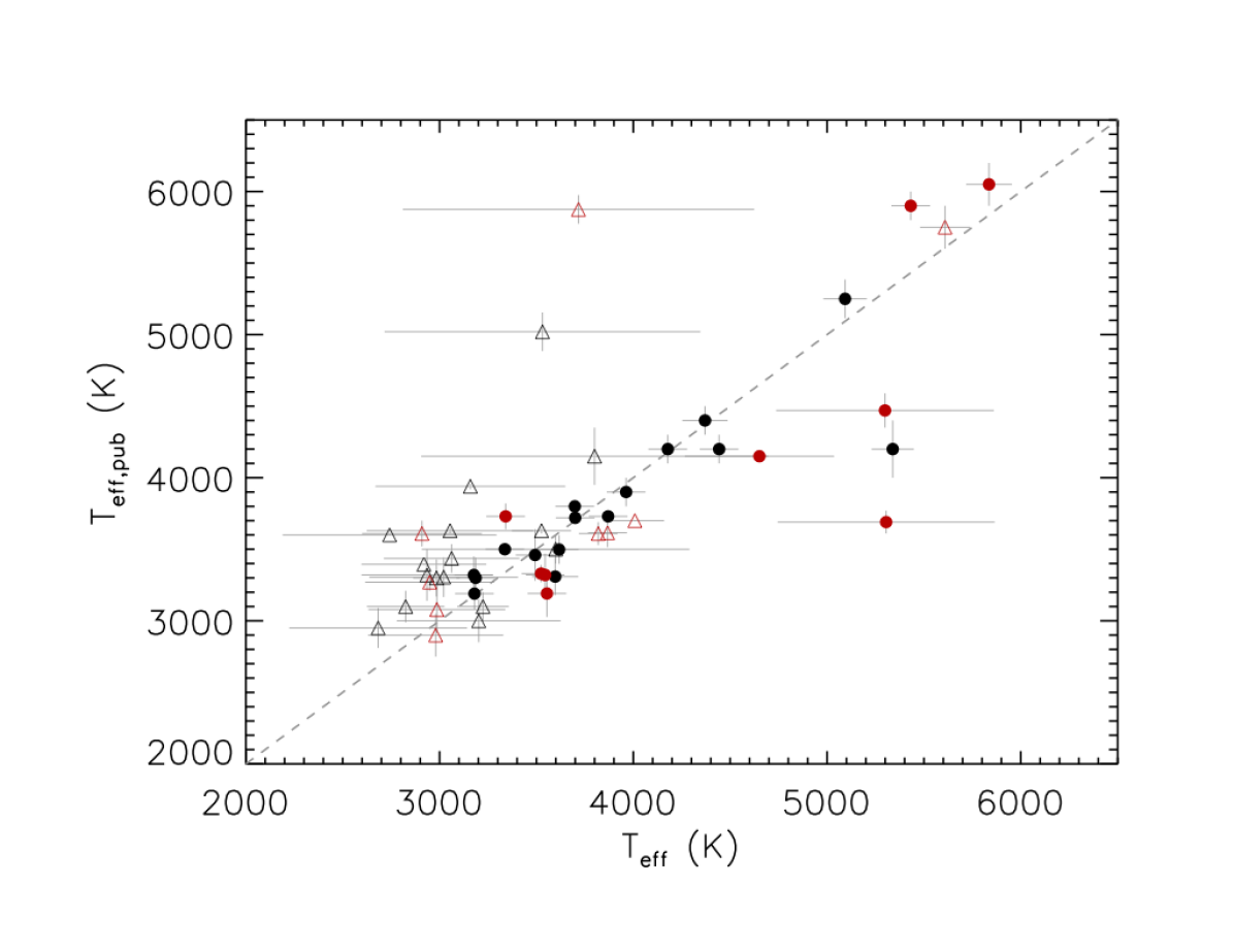
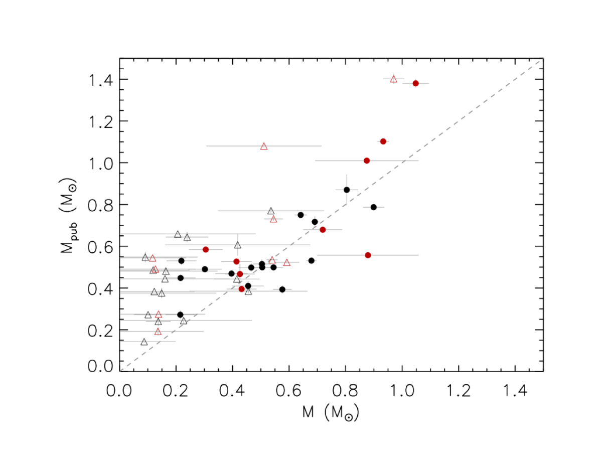
Figure 2: Comparison of obtained effective temperatures (left panel) and masses (right panel) for each EB component of the test sample with the literature values. Primary and secondary components are represented by filled circles and open triangles, respectively. The identified V+V systems are shown in black and the rejected systems are shown in red. The dashed line illustrates the identity function, for reference.

Once clusters and their members are defined, we then used the K-Nearest Neighbours classifiers (KNN, Cover & Hart, 1967; Chattopadhyay & Chattopadhyay, 2014) to characterise the systems according to their surrounding models. Considering fixed centroids for the observational data, the nearest synthetic data set were defined using euclidean distances in $\Re^{10}$, taking into account all ten colours of the grid. If sets of models from different EB pairs – V+V, III+V, and III+III – were present in a given cluster, the closest set was chosen based on the mean distance between the observational data and all the models in that given set. Hence, the closest set defines the class of our binaries. Since each synthetic binary (from models) already has temperatures defined for the primary and the secondary components, the effective temperature of our objects was determined as the mean $T_{\rm eff}$ value of their nearest surrounding models. The uncertainties in temperature were estimated by the standard deviation, as previously done in Garrido et al. (2019).

We applied the described procedure to a set of 24 known detached binaries from the literature, where 20 of them are V+V systems. Several of them were selected from the catalogue by Eker et al. (2014). We selected objects with available Pan-STARSS and 2MASS photometry, with stellar parameters derived from spectroscopic analysis. In general, the estimated effective temperatures are in agreement with literature values, within error estimates, as shown in table 1). The method was able to correctly assign the luminosity class for 16 known V+V systems.

We added to the test sample a binary system with a subgiant component – AN Cam (Southworth, 2021) – aiming at verifying how it would be treated by the method, since the grid of models was constructed with giant and dwarf stellar models only. The method was also successful in rejecting the AN Cam system, as it was identified as V+III, a binary with a giant component. The same way, we also analysed three other EBs, either with a substellar or a subdwarf component: 2MASSJ04463285+1901432 (Hebb et al., 2006), LSPM J1112+7626 (Irwin et al., 2011), and V1174 Ori (Stassun et al., 2004). Although having good $T_{\rm eff}$ estimates, these systems were also discarded by the method, being classified as V+III systems. Although the mentioned systems do not have a giant component, they were correctly discarded as non-V+V systems, being assigned this way probably because the model grid does not have models for substellar nor subdwarf objects included.

The method has misclassified as V+III and, hence, discarded, four known V+V systems, representing $20\%$ of the tested V+V set. We believe that was due to the unrealistic proportion between giant and dwarf models in the grid, as generated V+V systems represent only $\sim$1.3% of the model binaries. For this work, we used the most complete grid of models available by Bressan et al. (2012) to generate our grid – combining them in pairs to generate III+III, III+V, and V+V systems – and this is to be further improved as it misclassified some V+V systems. Nevertheless, this is not critical for our purpose, since we aimed at having a clean sample of V+V EB systems – i.e, free from giant contaminants – not focusing on the completeness of the analysed sample.

To have an estimate of the mass – hereafter, photometric mass – we interpolated the obtained temperatures with tabulated values using a forth-order polynomial fit. We adopted the values for effective temperatures and masses of main-sequence stars by Pecaut & Mamajek (2013), which is based on semi-empirical values. The photometric mass error estimates were calculated considering the $T_{\rm eff}$ uncertainties obtained with the KNN method. These values are also presented in table 1).

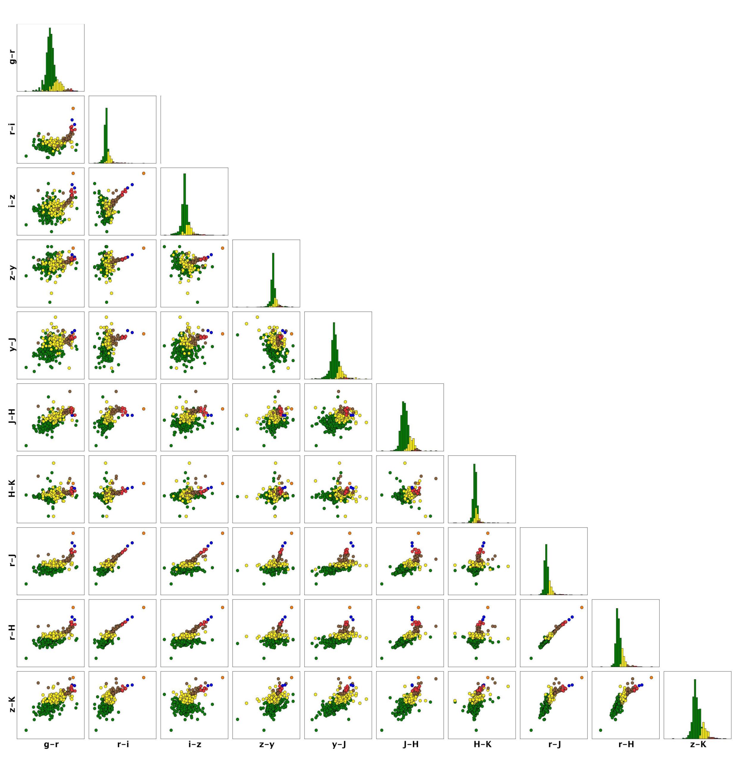
Figure 3: Distribution of the identified $493$ V+V EB systems in the adopted ten-colour grid, shown in colour cuts. The six clusters formed by the $k$-means method in which the V+V systems were distributed are represented here in different colours (as green, yellow, brown, red, blue, and orange bullets).

Figure 2 shows the comparison of the obtained values for the effective temperature and mass for each component of the test sample with published values (left and right panels, respectively). Primary components are presented as filled circles and secondary components as open triangles. The EBs correctly assigned as V+V systems are shown in black and the rejected systems – assigned by the method as V+III or III+III systems – are shown in red. The dashed line represents the identity function. For the estimated temperatures (left panel), a smaller dispersion is seen for the primaries in comparison to the estimated values for the secondaries. This is corroborated by the Pearson correlation coefficient ($r$) of 0.82 and 0.78 for the primary and the secondary components, respectively. It is worth noting that larger $T_{\rm eff}$ uncertainties were estimated of the secondaries. A similar behavior is shown for the estimated photometric masses (fig. 2, right panel), with $r$ of 0.78 and 0.76 for the primary and the secondary components, respectively. As expected, we obtained larger errors in this case, nevertheless, presenting a good agreement with the values from literature, considering the estimated uncertainties (see table 1). Differences with published values are more notorious for low temperature and mass values – $T_{\rm eff}<3500$ K and $M_{\star}<0.4$ M_⊙ – especially for secondary components. This behaviour was expected, as we used only the information coming from broad-band photometry where a low-mass secondary component would contribute less in the binary integrated flux. Moreover, there could be a limitation due to the adopted colours, since we do not explore the infrared region.

Intrinsic stellar variability, due to starspots for instance, could affect the adopted single-epoch photometric measurements from Pan-STARRS and 2MASS, which could lead to a wrong classification by the method and/or erroneous temperature and mass estimations. Independently of the assigned classification, some temperatures were estimated by the method with large error bars, which could indicate inconsistencies among the photometric data when compared to the models. For instance, some of the outliers in figure 2 are systems with observed stellar variability probably due to starspots. This is the case, for example, of AN Cam (Southworth, 2021) and V1174 Ori (Stassun et al., 2004), where the observed light curve variability showed strong evidences of spot activity.

We then performed the KNN method for the initial sample with $821$ EB systems, regardless their LC morphology. The model binaries with only dwarf stars as components were present in six of the $17$ clusters formed by the $k$-means method, meaning that only the observed binaries within these clusters could be assigned as V+V systems. As a result, we found that $493$ EBs from our selected sample were defined as V+V systems. The remaining systems were discarded by the method, nevertheless, as mentioned previously, this does not mean they have giant components. For example, the EB KIC08736245 system is a previously known system with solar-type components leaving the main sequence (Fetherolf et al., 2019), and it was correctly discarded by our method, as it could not be classified as a V+V system. As mentioned previously, the used single-epoch photometric measurements may be affected by intrinsic variability, for example due to starspots, which could lead to an incorrect classification. Therefore, some detached V+V systems may have been discarded by the method. Nevertheless, the main objective of this work was to select a sample clean from evolved components, not aiming at having a complete subset of detached V+V binaries.

Among the identified V+V systems, the obtained $T_{\rm eff}$ vary from $3\,152$ to $5\,991$ K for primary components and from $2\,632$ to $5\,991$ K for the secondaries. Note that the highest estimated temperature ($5\,991$ K) is the upper $T_{\rm eff}$ limit of our model grid. All colour cuts are presented in fig. 3, showing the distribution of V+V systems in six of the clusters formed by the $k$-means method, where each cluster is represent by a different colour (as green, yellow, brown, red, blue, and orange bullets).

Correlating the V+V EBs found by the KNN method with those systems identified as detached binaries according to their LC morphology (the adopted criteria are described in Sect. 2), we gathered a final list with $164$ detached systems with only main-sequence stars. The derived photometric masses and effective temperatures for all $330$ stars (both components of the $164$ V+V DEB systems) are presented in tables 2, 3, and 4, in Appendix A. For example, the estimated temperatures for the components of EB KIC12109845 are of $4\,612$ and $3\,971$ K for the primary and secondary components, respectively. This system was previously described as a detached system composed by a late K and an early M stars (Harrison et al., 2012).

We compared estimated temperatures with the values from Armstrong et al. (2014). Among the $148$ systems in common to their study, in general these authors estimated higher temperatures for primary and secondary components, as shown in figure 4 (top panel). As mentioned before, our highest estimated temperature was limited to $5\,991$ K, the hottest dwarf model used in our grid. Some of the comparison temperatures are above $8\,000$ K. The agreement between both approaches is also presented (fig. 4, bottom panel) in a Bland-Altman plot, illustrating the difference between the results from Armstrong et al. (2014) and ours. The black and grey solid lines show that the mean $T_{\rm eff}$ difference ($T_{\rm eff,thiswork}-T_{\rm eff,pub}$) is approximately of $-486$ and $-1033$ K for primaries and secondaries, respectively. Dashed lines show the 2-sigma interval for a 95% confidence level.

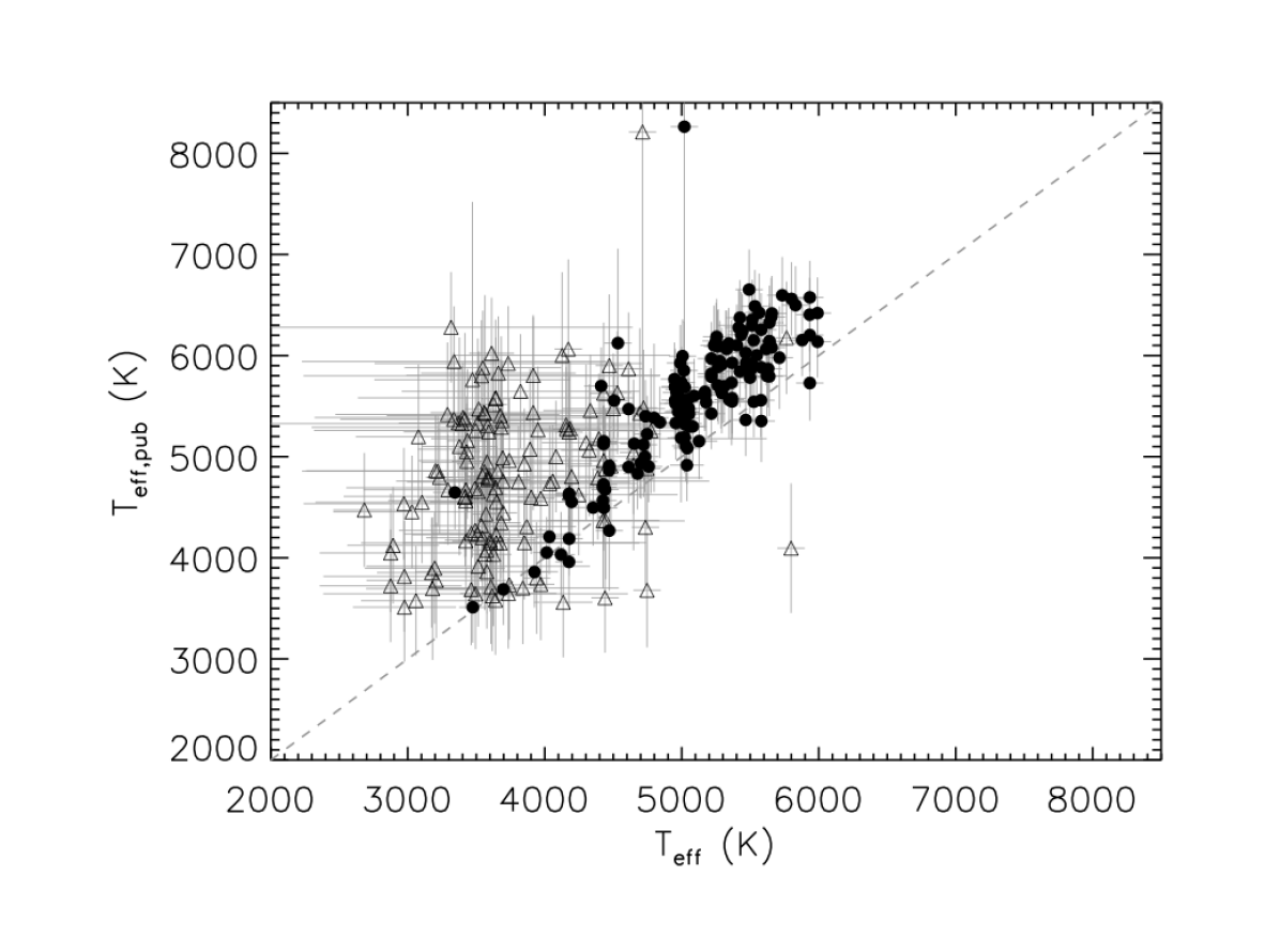
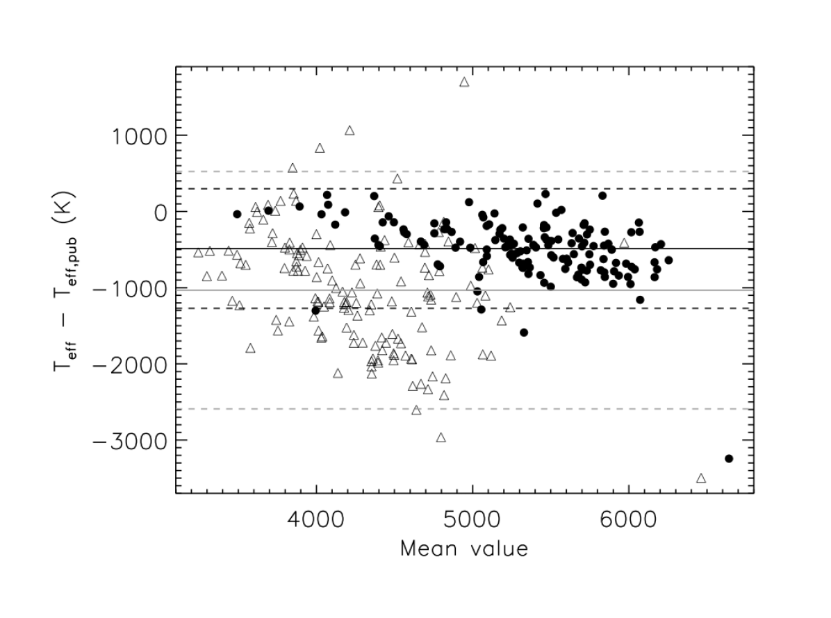
Figure 4: Comparison between effective temperatures obtained in this work with the literature values from Armstrong et al. (2014). Top panel: Our estimated $T_{\rm eff}$ for each Kepler DEB component are shown in the horizontal axis and the literature values are presented in the vertical axis. Primary and secondary components are represented by filled circles and open triangles, respectively. The dashed line illustrates the identity function. Bottom panel: The Bland-Altman plot, showing the agreement between both methods. The horizontal axis shows the mean value between the results from Armstrong et al. (2014) and ours, and the vertical axis shows the difference between them. The mean $T_{\rm eff}$ difference for primaries and secondaries are shown as black and grey solid lines, respectively. Dashed lines illustrate the 2-sigma interval.

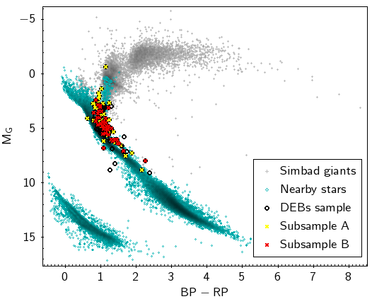
Figure 5: Colour-magnitude diagram of our sample of DEB candidates (black open circles). The overplotted subsamples A and B represent systems with radii values estimated from light-curve fitting (see Sect. 5 for details). Nearby main-sequence objects (within $\sim 100$ pc) identified from Gaia EDR3 are shown as cyan diamonds. A sample of SIMBAD giant stars are shown as gray crosses.

3.2 Searching for giant contaminants

We searched for giant contaminants within our final sample of $164$ DEBs by comparing our objects to a set of dwarf and giant stars in a colour-magnitude diagram (CMD).

We used the SIMBAD Astronomical Database (Wenger et al., 2000) to find a representative sample of objects classified as giant stars, with spectral types ranging from F to M type. With the help of TOPCAT (Taylor, 2005, 2011), we searched for the available Gaia parallaxes and photometry by cross-matching the set of giant stars within $5\arcsec$ with the Gaia Early Data Release 3 (Gaia EDR3; Gaia Collaboration et al., 2016, 2021, epoch 2016). A second set of comparison was defined from the Gaia EDR3, searching for nearby objects with parallax greater than $10$ mas (within $\sim 100$ pc). From both sets, giant stars from SIMBAD and nearby stars from Gaia, we kept only those objects that presented Gaia parallax error of less than $10$%, with errors in all Gaia magnitudes ($G$, $BP$, and $RP$ bands) of less than $5$%, and with the Renormalised Unit Weight Error (RUWE) of less than $1$, which is the value expected for single stars (Arenou et al., 2018; Lindegren et al., 2018, 2021).

To have a clear distribution of comparison stars in the main sequence, we firstly estimated the corrected $BP$ and $RP$ flux excess factor, $C^{*}$, which is a quality metric according to their $(BP-RP)$ colours, defined by Riello et al. (2021). In figure 5, the greenish diamonds represent the sample of Gaia nearby stars which have $|C^{*}|<\sigma$, where $\sigma$ is the $C^{*}$ scatter as function of $G$ magnitude. The sample of giant stars from SIMBAD are shown in fig. 5, represented by gray crosses.

We also cross-matched our sample ($164$ DEBs) with Gaia EDR3, where we found good photometric data (errors within $5$%) for $161$ systems. These objects are presented in figure 5 as black open circles. The overplotted subsamples A and B (shown as yellow and red crosses, respectively) represent those systems with radii estimates from LC modeling, which will be explained later in Section 5. Note that the majority of our EBs have $(BP-RP)$ colour – combined for the system – redder than $0.983$, which is the expected value for a K0 V star according to Pecaut & Mamajek (2013).

4 Light-curve modelling with JKTEBOP and AGA

We have identified $300$ objects from the Kepler EBs Catalog – considering the criteria described in Sect. 2 – as short-period detached systems. However, after applying the KNN method (described in Sect. 3.1), only $164$ DEB candidates were classified as $V+V$ systems. For this sample of $V+V$ DEBs, we performed the fitting of Kepler LCs using the JKTEBOP code (Southworth et al., 2004; Southworth, 2013), which uses the Nelson–Davis–Etzel model (NDE model; Nelson & Davis, 1972; Popper & Etzel, 1981) and is suitable for detached systems. To help dealing with such long time series – Kepler light curves can have tens of thousands epochs – we adopted the asexual genetic algorithm (AGA) by Cantó et al. (2009), which was implemented to the JKTEBOP code by Coughlin et al. (2011), and already was successfully applied for hundreds of detached EBs found in the CSS (for more details, see Garrido et al. (2019)).

We calculated the stellar measured flux ($F_{\rm obs}$) from the median flux in each quarter of observations, as shown below:

$$F_{\rm obs}=\sum_{Q=1}^{n}F_{\rm Q}\frac{N_{\rm Q}}{N_{\rm tot}},$$ (1)

where ($F_{\rm Q}$) is the median flux observed in a given quarter, $N_{\rm Q}$ is the number of observations (epochs) in that quarter, $N_{\rm tot}$ is the total number of epochs, and $n$ is the last observed quarter. Note that the maximum value for $n$ is $18$, which is the number of quarters observed during the Kepler mission. However, not all stars have data for all quarters. We obtained the analysed LCs in magnitudes by adopting the zero point given by the Kepler team, where the empirical flux for a star with Kepler magnitude of $Kp=12$ mag is of $1.74\times 10^{5}$ e^-/s.

Light curve models provide information on the radius of each component in addition to the orbital configuration of the studied systems. For the modelling, the following parameters were free to vary in the first approach:

• the orbital period ($P_{\rm orb}$),

• the reference time (epoch) of primary minimum ($T_{\rm 0}$),

• the sum of the stellar radii ($r_{1}+r_{2}$),

• the ratio of the radii ($r_{2}/r_{1}$),

• the central surface brightness ratio ($J=J_{2}/J_{1}$),

• the orbital inclination ($i$),

• the orbital eccentricity ($ecc$), and

• the baseline level of the light curve,

where $P_{\rm orb}$ and $T_{\rm 0}$ are given in days, $r_{1}+r_{2}$ is given in units of the binary separation, $i$ in degrees, and the baseline level in Kepler magnitudes.

We adopted $P_{\rm orb}$ and $T_{\rm 0}$ values from the KEBC catalogue as initial conditions. We assumed that the argument of periastron ($\omega$) to be null, as it may be not well constrained. We also assumed no third light source in the binary light curve. The photometric mass ratio ($q$) was calculated from the previously obtained photometric masses (sect. 3.1) and it was kept fixed, as it is used by the code only to determine possible tidal deformation on the components.

Limb-darkening (LD) coefficients were estimated with the JKTLD procedure, considering the temperatures obtained for each component (see sect. 3.1). We adopted a quadratic LD law with coefficients from Claret (2000). Both LD coefficients were used as fixed parameters in the modelling procedure with JKTEBOP. Gravity darkening coefficients were also kept fixed to $0.32$, which is the typical value for stars with convective envelopes (Lucy, 1967). The reflection coefficients were also fixed in the fitting, calculated by the code based on the system geometry.

The fitting was performed iteratively. Some LCs presented non-negligible baseline variation over time – for example due to spots – easily identified in the phase-folded light curve containing the complete data set. Since the time-series data can have up to four years of observations, it may affect the eclipse relative depth and the results from light-curve modelling.

Therefore, we adopted a second approach considering only one quarter of observations – Kepler observations were divided in $90$-day quarters. We chose the quarter with the highest number of epochs observed for each binary. The fitting with JKTEBOP was performed considering the same variables and assumptions described above, with the exception of $P_{\rm orb}$, which was kept as a fixed value. This is a good assumption too as the orbital period have been already defined with a good precision (Kirk et al., 2016, and references therein). This is also a robust approach based on a minimum set of free parameters, which are more reliable within a quarter.

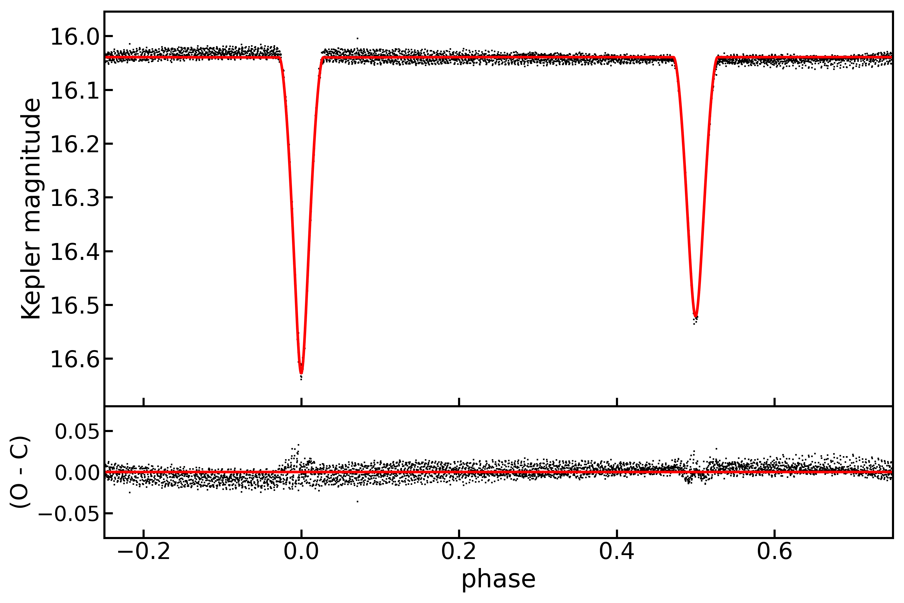
Figure 6: Phase-folded light curve of EB KIC09656543 (tenth quarter). Black dots are the observed data, in Kepler magnitudes. The red solid line shows the best-fitting model from the JKTEBOP code.

Convergence was achieved for $94$ DEB systems after four complete iterations. We then performed a Monte Carlo (MC) analysis – a task included in the JKTEBOP code – with $10\,000$ iterations per LC, for a robust uncertainties estimation. The obtained set of parameters are shown in tables 5 and 6, in Appendix B. As an example, the phase-folded light curve of KIC09656543 is shown in fig. 6, where we adopted phase zero for the primary eclipse minimum. The best-fitting model is represented by a red solid line.

For these systems, and with the objective of exploring the mass-radius relationship (see Sect. 5), we have estimated their radius values, in units of the solar radius ($R_{\odot}$). The LC-fitting code gives $r_{1}+r_{2}$ and $r_{2}/r_{1}$ – the sum and the ratio of the stellar radii, respectively – in units of the binary separation ($a$). To obtain the radii in $R_{\odot}$, we adopted Kepler’s Third law to calculate $a$, using the known orbital period and previously derived photometric masses of both components.

Almost half of these systems presented large error estimates for the photometric masses for the secondary components (with a mean relative error of 62.9%, approximately), which led to large uncertainties on the calculated radius and a large discrepancy from the expected mass-radius relation for main-sequence stars. As mentioned previously, these uncertainties could be related to the the adopted single-epoch photometric measurements, which in turn could be affected by intrinsic stellar variability (see Sect. 3.1). These systems are represented in fig. 5 by yellow crosses (subsample A). Some of them could have a subgiant component that was not correctly identified by our method based on our ten-colour grid of models. Nevertheless, we believe this is not the general case, as the mentioned EBs are well positioned in the colour-magnitude diagram and have RUWE < 1.4 (for more details, see Sect. 3.2).

Subsample B contains the remaining DEB systems, which in general presented more reliable photometric mass solutions – the estimated mean relative mass errors for the secondary components are of $\sim$25.5%. They are shown in figure 5 as red crosses. These objects are discussed below, in section 5.

The majority of the non-converged systems presented high variability in the analysed light curve and/or have shallow secondary eclipses. If the LC present intense out-of-eclipse variability, due to stellar spots for instance, they can introduce systematic errors in the LC analysis. In this case, the fitting process may be problematic, especially for low-mass stars with spotted surfaces, since they can result in deeper eclipses or mislead the surface brightness estimation, resulting in wrong $r_{1}+r_{2}$ and $r_{2}/r_{1}$ values (e.g. Irwin et al., 2011). Moreover, the presence of such an intrinsic variability during the eclipse ingress/egress may lead to erroneous radii solutions. Under such circumstances, we do not neglect the possibility of cross talk between some of the fitting parameters. Therefore, those systems were rejected on the basis of inconsistent light curve solutions.

5 Discussion

Prša et al. (2011) – and the update by Slawson et al. (2011) – have presented the first EB catalogue from Kepler database, where they have estimated some orbital parameters like $P_{\rm orb}$, eccentricity and argument of periastron ($e\cos{\omega}$, $e\sin{\omega}$). Comparing the analysed sample in this work to their solutions, the majority of them present small eccentricity values, which are consistent in general with our results. They also obtained $r_{1}+r_{2}$ values, the fitting solution for the sum of the stellar radii for the studied systems. The majority of our estimated values are in agreement with those from Slawson et al. (2011). For comparison, these values are also presented in Appendix B (tables 5, and 6).

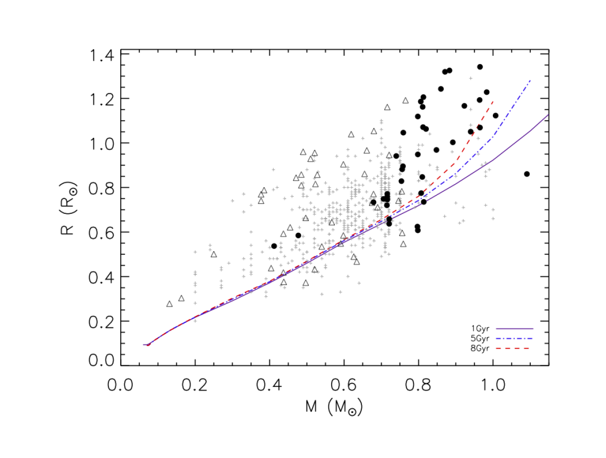
Figure 7: Mass radius diagram for the DEB systems in subsample B. Primary and secondary components are represented by filled circles and open triangles, respectively. Baraffe et al. (2015) standard stellar models ($[M/H]$ = 0, $Y$ = 0.28, $L_{\rm mix}=1.6HP$) for $1$, $5$, and $8$ Gyr are represented by solid, dot-dashed, and dashed lines, respectively. DEB candidates from the CSS (Garrido et al., 2019) are illustrated as small gray crosses.

5.1 The mass-radius diagram

In order to search for a general trend among the obtained parameters for the DEBs in subsample B, we displayed the radii and masses derived for each binary component in a mass-radius diagram, presented in figure 7. The open circles and triangles represent the primary and the secondary components, respectively.

There seems to be a general trend of radii inflation among our objects, where we derived radii values larger than predicted by stellar evolutionary models, despite the individual uncertainties. The standard models from Baraffe et al. (2015) for 1, 5, and 8 Gyr – computed considering a solar metallicity ($[M/H]$ = 0), with a helium abundance of $Y$ = 0.28, and for a convective mixing length equal to the scale height ($L_{\rm mix}=1.6HP$) – are also illustrated in figure 7. For comparison, the results from Garrido et al. (2019) are shown as small gray crosses. We observe that the cloud of points is similarly scattered, as in Garrido et al. (2019), which may be the result of the larger individual uncertainties obtained by adopting a purely-photometric method (in comparison to smaller errors that can be achieved with spectroscopic methods). It is worth mentioning that other parameters, such as metallicity and age, may also affect the exact locus of individual stars in the mass-radius diagram.

The average difference between the measured stellar radius and expected value for the 5-Gyr model from Baraffe et al. (1998) – as an estimate of the radius inflation – appears to be larger for the secondary than for primary components, by over 20% more inflated. A similar value is estimated from the CSS sample analysed in Garrido et al. (2019) (Fig. 7, gray crosses).

More detailed studies of the final sample presented here, as well as the sample outlined in Garrido et al. (2019) are important to the understanding of the radius inflation. Further search for correlations between the measured inflation and metallicity, age, stellar activity, and/or rotation may hold clues to the mechanism behind the mass-radius anomaly. It may be also important to investigate the possible effects that the adopted sample selection or methodology may have on the obtained results. Interestingly, a recent search for DEBs in CSS database by Carmo et al. (2020) shows no significant inflation among selected targets. We understand the difficulties on deriving stellar physical parameters without spectroscopic data and on developing a model-independent analysis based only on photometry. Therefore, we believe the incongruities found rely on the sample properties, their selection effects and analysis methods.

One may expect a smaller scatter of our DEB systems in the mass-radius diagram when compared to that from CSS, due to the superb Kepler light curves, which should lead to smaller uncertainties in the estimated stellar radii. However, it is difficult to probe the intrinsic scatter of mass and radii values in both samples. On the other hand, the superb light curves from Kepler allowed us to resolve other features, such as modulations due to spots for example. This may have an effect on the derived parameters and limit the expected precision, leading to larger uncertainties, as discussed previously.

Our objective was to study homogeneously the whole sample, rejecting unreliable or biased mass or radius estimates, not dealing with each system individually. For instance, removing the contribution due to spots may improve the radius estimation, however, it may require a case-by-case, time-dependent spot mapping analysis. Further improvements in the light curve analysis will be implemented in order to achieve better radii estimates, i.e. with smaller uncertainties.

6 Conclusions

We presented the characterisation of detached eclipsing binary systems from the Kepler field with low mass components by adopting a purely-photometric method.

Effective temperatures and photometric masses of individual components we estimated from an extensive multi-colour dataset. We adopted machine learning clustering techniques for the analysis, using a ten-colour binary model grid constructed from the evolutionary stellar models by Bressan et al. (2012), considering Pan-STARRS and 2MASS broad-band filters. For this new grid, we used a different set of colours (based on the available photometric bands) to generate a more complete set of model binary – with over $180\,000$ models – which allowed a better temperature determination than done previously in Garrido et al. (2019).

For primary components, we obtained temperatures from $3\,152$ to $5\,991$ K, and from $2\,632$ to $5\,991$ K for the secondaries. Differences with published values are greater towards lower temperatures and masses ($T_{\rm eff}<3500$ K; $M_{\star}<0.4$ M_⊙), especially for secondary components, as expected. We intend to explore and add new colours to our grid, covering the infrared region in order to improve the efficiency of our method for binary components in the mentioned low-mass regime.

Previous works also adopted a purely-photometric methodology to derive stellar physical parameters of EB components, using for instance stellar models, available broad-band photometric data and light-curve fitting procedures. Devor et al. (2008) have derived stellar properties from photometric data, although they relied on isochrones for the stellar mass estimation. Windemuth et al. (2019) adopted a similar approach, using Gaia distances as a stellar model constraint. Differently in this work, we adopted semi-empirical values to derive stellar masses. For those systems in common with the sample analysed by Windemuth et al. (2019), we found a good agreement for the estimated masses, where the median difference is of 20% for the primary and 45% for the secondary components, approximately.

We also estimated the radii and orbital parameters from the available Kepler light curves for $104$ detached EB systems. For that, we used the JKTEBOP code (Southworth et al., 2004; Southworth, 2013) modified by Coughlin et al. (2011) with the asexual genetic algorithm (AGA) by Cantó et al. (2009). Spurious values from light-curve modelling were used to reject systems showing high variability – for instance, due to stellar spots – and/or eventual subgiant components. Future analysis may account for variability in order to find reliable estimates for such cases.

Despite large individual uncertainties, our results show that there is an inflation trend (of $\approx 20\%$) observed in a mass-radius diagram against theoretical stellar models for low mass regime ($M<1.0$ M_⊙). Nevertheless, additional case-by-case analysis, with spectroscopic masses based on single-target radial velocity measurements, are important to set new boundaries to the problems and further investigate the causes of the radius anomaly in low-mass components of detached EB systems.

Data Availability

The analysed light curves were obtained directly from Kepler mission archive, available at https://archive.stsci.edu/missions/kepler/lightcurves/.

Appendix A Derived effective temperatures and masses for the 164 identified DEB systems.

We present from table 2 to 4, the derived parameters for the sample of $164$ DEBs identified from the KEBC. The first column shows the Kepler identification (KIC), followed by the estimated effective temperatures and the masses of each component, which were obtained from a ten-colour grid models, as described in detail in Sect. 3.

Table 2: Derived effective temperatures and masses for the components of the $164$ identified DEB systems from the Kepler survey. $T_{1}$ and $M_{1}$ are the $T_{\rm eff}$ and the stellar mass obtained for the primary component. $T_{2}$ and $M_{2}$ are the estimated values for the secondary.

KIC	$\mathrm{T}_{1}$ (K)	$\mathrm{M}_{1}$ (M⊙)	$\mathrm{T}_{2}$ (K)	$\mathrm{M}_{2}$ (M⊙)
1575690	4034 $\pm$ 100	0.650 $\pm$ 0.021	3208 $\pm$ 509	0.236 $\pm$ 0.324
2308957	5006 $\pm$ 100	0.809 $\pm$ 0.023	3661 $\pm$ 565	0.531 $\pm$ 0.155
2447893	4972 $\pm$ 100	0.802 $\pm$ 0.022	3202 $\pm$ 944	0.232 $\pm$ 0.441
2854948	5292 $\pm$ 107	0.882 $\pm$ 0.032	4694 $\pm$ 355	0.752 $\pm$ 0.066
2856960	4677 $\pm$ 100	0.750 $\pm$ 0.016	3579 $\pm$ 482	0.483 $\pm$ 0.173
3122985	5364 $\pm$ 100	0.910 $\pm$ 0.024	3563 $\pm$ 294	0.472 $\pm$ 0.127
3218683	4412 $\pm$ 124	0.714 $\pm$ 0.016	3416 $\pm$ 283	0.371 $\pm$ 0.181
3241344	5343 $\pm$ 135	0.902 $\pm$ 0.037	3495 $\pm$ 1112	0.426 $\pm$ 0.314
3338660	5236 $\pm$ 100	0.866 $\pm$ 0.029	3424 $\pm$ 100	0.377 $\pm$ 0.069
3344427	4429 $\pm$ 100	0.716 $\pm$ 0.013	3646 $\pm$ 382	0.523 $\pm$ 0.125
3656322	5022 $\pm$ 100	0.813 $\pm$ 0.023	3546 $\pm$ 124	0.461 $\pm$ 0.076
3659940	5368 $\pm$ 100	0.911 $\pm$ 0.024	4180 $\pm$ 100	0.679 $\pm$ 0.016
3662635	5328 $\pm$ 109	0.892 $\pm$ 0.033	4775 $\pm$ 323	0.765 $\pm$ 0.065
3730067	4119 $\pm$ 100	0.668 $\pm$ 0.018	3181 $\pm$ 486	0.220 $\pm$ 0.315
3834364	5640 $\pm$ 100	0.979 $\pm$ 0.046	4443 $\pm$ 100	0.718 $\pm$ 0.013
3848919	4952 $\pm$ 100	0.798 $\pm$ 0.022	4082 $\pm$ 693	0.661 $\pm$ 0.104
3848972	5526 $\pm$ 100	0.953 $\pm$ 0.034	4501 $\pm$ 376	0.725 $\pm$ 0.058
3853673	5622 $\pm$ 147	0.974 $\pm$ 0.060	4127 $\pm$ 788	0.670 $\pm$ 0.121
3973002	5580 $\pm$ 113	0.965 $\pm$ 0.044	3916 $\pm$ 928	0.619 $\pm$ 0.158
4069063	5934 $\pm$ 100	1.090 $\pm$ 0.023	4530 $\pm$ 102	0.729 $\pm$ 0.014
4073678	5277 $\pm$ 100	0.877 $\pm$ 0.029	3682 $\pm$ 1384	0.543 $\pm$ 0.280
4078693	5216 $\pm$ 100	0.860 $\pm$ 0.028	3698 $\pm$ 100	0.551 $\pm$ 0.038
4174507	5425 $\pm$ 100	0.929 $\pm$ 0.024	3741 $\pm$ 662	0.570 $\pm$ 0.143
4357272	5022 $\pm$ 103	0.813 $\pm$ 0.024	3419 $\pm$ 887	0.373 $\pm$ 0.326
4386047	5016 $\pm$ 100	0.811 $\pm$ 0.023	3511 $\pm$ 577	0.437 $\pm$ 0.225
4480676	5052 $\pm$ 100	0.819 $\pm$ 0.024	3538 $\pm$ 1299	0.455 $\pm$ 0.320
4484356	4951 $\pm$ 100	0.798 $\pm$ 0.022	3232 $\pm$ 100	0.250 $\pm$ 0.064
4551328	5080 $\pm$ 100	0.826 $\pm$ 0.025	3496 $\pm$ 1181	0.427 $\pm$ 0.323
4670267	5640 $\pm$ 100	0.979 $\pm$ 0.046	4612 $\pm$ 100	0.740 $\pm$ 0.015
4681152	5534 $\pm$ 100	0.955 $\pm$ 0.035	3514 $\pm$ 816	0.439 $\pm$ 0.263
4757331	5021 $\pm$ 100	0.812 $\pm$ 0.023	3432 $\pm$ 107	0.382 $\pm$ 0.074
4826439	5935 $\pm$ 100	1.091 $\pm$ 0.023	5765 $\pm$ 100	1.017 $\pm$ 0.047
4840263	5255 $\pm$ 100	0.871 $\pm$ 0.029	3591 $\pm$ 622	0.490 $\pm$ 0.194
4902030	4196 $\pm$ 100	0.682 $\pm$ 0.016	2975 $\pm$ 591	0.130 $\pm$ 0.344
4908495	4759 $\pm$ 100	0.762 $\pm$ 0.017	3294 $\pm$ 618	0.288 $\pm$ 0.329
5017058	5991 $\pm$ 100	1.117 $\pm$ 0.010	3316 $\pm$ 1325	0.303 $\pm$ 0.442
5018787	5216 $\pm$ 100	0.860 $\pm$ 0.028	3901 $\pm$ 100	0.614 $\pm$ 0.028
5022440	5515 $\pm$ 145	0.951 $\pm$ 0.048	3642 $\pm$ 1091	0.521 $\pm$ 0.237
5036538	4431 $\pm$ 100	0.716 $\pm$ 0.013	3538 $\pm$ 373	0.455 $\pm$ 0.162
5039441	5492 $\pm$ 100	0.946 $\pm$ 0.030	3625 $\pm$ 131	0.511 $\pm$ 0.065
5215700	5466 $\pm$ 100	0.940 $\pm$ 0.027	3338 $\pm$ 1111	0.317 $\pm$ 0.401
5218441	5267 $\pm$ 100	0.874 $\pm$ 0.029	3417 $\pm$ 124	0.372 $\pm$ 0.086
5636642	4947 $\pm$ 100	0.797 $\pm$ 0.022	4721 $\pm$ 100	0.756 $\pm$ 0.016
5649956	5216 $\pm$ 100	0.860 $\pm$ 0.028	3557 $\pm$ 100	0.468 $\pm$ 0.061
5785586	5044 $\pm$ 100	0.817 $\pm$ 0.024	4445 $\pm$ 577	0.718 $\pm$ 0.095
5802470	5498 $\pm$ 100	0.947 $\pm$ 0.030	3646 $\pm$ 616	0.523 $\pm$ 0.169
5802486	5467 $\pm$ 100	0.940 $\pm$ 0.027	4185 $\pm$ 228	0.680 $\pm$ 0.034
6047498	5333 $\pm$ 107	0.893 $\pm$ 0.033	4123 $\pm$ 758	0.669 $\pm$ 0.115
6058875	4429 $\pm$ 100	0.716 $\pm$ 0.013	3655 $\pm$ 100	0.528 $\pm$ 0.047
6103049	5617 $\pm$ 100	0.973 $\pm$ 0.044	4333 $\pm$ 343	0.703 $\pm$ 0.047
6182019	5296 $\pm$ 100	0.883 $\pm$ 0.030	3601 $\pm$ 330	0.497 $\pm$ 0.127
6187341	4665 $\pm$ 100	0.748 $\pm$ 0.015	3166 $\pm$ 715	0.212 $\pm$ 0.396
6209347	5368 $\pm$ 100	0.911 $\pm$ 0.024	4158 $\pm$ 100	0.675 $\pm$ 0.017
6283224	5178 $\pm$ 100	0.850 $\pm$ 0.027	4196 $\pm$ 333	0.682 $\pm$ 0.047
6311681	5084 $\pm$ 100	0.827 $\pm$ 0.025	3585 $\pm$ 1182	0.486 $\pm$ 0.278
6452742	5443 $\pm$ 100	0.934 $\pm$ 0.025	4396 $\pm$ 1225	0.711 $\pm$ 0.274
6469946	5040 $\pm$ 100	0.817 $\pm$ 0.024	4648 $\pm$ 100	0.746 $\pm$ 0.015
6516874	5503 $\pm$ 100	0.948 $\pm$ 0.031	3612 $\pm$ 164	0.503 $\pm$ 0.079
6531485	5321 $\pm$ 103	0.890 $\pm$ 0.031	3823 $\pm$ 867	0.594 $\pm$ 0.157
6543674	5509 $\pm$ 100	0.949 $\pm$ 0.032	3548 $\pm$ 572	0.462 $\pm$ 0.206
6545018	5547 $\pm$ 100	0.957 $\pm$ 0.036	3642 $\pm$ 1007	0.521 $\pm$ 0.225
6595662	5581 $\pm$ 100	0.965 $\pm$ 0.040	3641 $\pm$ 100	0.521 $\pm$ 0.049
6620003	3925 $\pm$ 100	0.622 $\pm$ 0.026	3174 $\pm$ 399	0.217 $\pm$ 0.262
6665064	5640 $\pm$ 100	0.979 $\pm$ 0.046	3971 $\pm$ 100	0.634 $\pm$ 0.024
6695889	5801 $\pm$ 100	1.031 $\pm$ 0.045	3607 $\pm$ 158	0.500 $\pm$ 0.079
6697716	4735 $\pm$ 100	0.759 $\pm$ 0.017	4735 $\pm$ 100	0.759 $\pm$ 0.017
6706287	4998 $\pm$ 100	0.807 $\pm$ 0.023	3624 $\pm$ 100	0.510 $\pm$ 0.052
6778050	5054 $\pm$ 100	0.820 $\pm$ 0.024	4178 $\pm$ 100	0.679 $\pm$ 0.016
6862603	5654 $\pm$ 103	0.983 $\pm$ 0.047	3892 $\pm$ 819	0.611 $\pm$ 0.144
6863840	5030 $\pm$ 100	0.814 $\pm$ 0.024	3851 $\pm$ 494	0.598 $\pm$ 0.106

Table 3: Continued from Table 2.

KIC	$\mathrm{T}_{1}$ (K)	$\mathrm{M}_{1}$ (M⊙)	$\mathrm{T}_{2}$ (K)	$\mathrm{M}_{2}$ (M⊙)
7025540	4429 $\pm$ 100	0.716 $\pm$ 0.013	3602 $\pm$ 377	0.497 $\pm$ 0.139
7174617	4957 $\pm$ 100	0.799 $\pm$ 0.022	3577 $\pm$ 100	0.481 $\pm$ 0.059
7212066	5262 $\pm$ 100	0.873 $\pm$ 0.029	3682 $\pm$ 141	0.543 $\pm$ 0.052
7220320	5251 $\pm$ 100	0.870 $\pm$ 0.029	3584 $\pm$ 100	0.486 $\pm$ 0.058
7295570	5169 $\pm$ 100	0.848 $\pm$ 0.027	3337 $\pm$ 100	0.317 $\pm$ 0.069
7374746	5019 $\pm$ 100	0.812 $\pm$ 0.023	4714 $\pm$ 100	0.755 $\pm$ 0.016
7377033	4984 $\pm$ 100	0.804 $\pm$ 0.022	4747 $\pm$ 100	0.761 $\pm$ 0.017
7552344	5012 $\pm$ 100	0.810 $\pm$ 0.023	3290 $\pm$ 818	0.286 $\pm$ 0.380
7605600	3698 $\pm$ 100	0.551 $\pm$ 0.038	3060 $\pm$ 401	0.162 $\pm$ 0.241
7671594	3344 $\pm$ 159	0.321 $\pm$ 0.111	2893 $\pm$ 335	0.108 $\pm$ 0.139
7769072	4653 $\pm$ 100	0.746 $\pm$ 0.015	3648 $\pm$ 486	0.524 $\pm$ 0.147
7798259	4721 $\pm$ 100	0.756 $\pm$ 0.016	3941 $\pm$ 100	0.626 $\pm$ 0.026
7830321	5169 $\pm$ 100	0.848 $\pm$ 0.027	3518 $\pm$ 100	0.442 $\pm$ 0.065
7842610	5142 $\pm$ 133	0.841 $\pm$ 0.036	3659 $\pm$ 1123	0.531 $\pm$ 0.236
7947631	4841 $\pm$ 100	0.776 $\pm$ 0.019	3577 $\pm$ 519	0.481 $\pm$ 0.182
8094140	4177 $\pm$ 100	0.679 $\pm$ 0.016	3463 $\pm$ 285	0.404 $\pm$ 0.169
8097825	5262 $\pm$ 100	0.873 $\pm$ 0.029	3640 $\pm$ 100	0.520 $\pm$ 0.050
8111381	5473 $\pm$ 110	0.941 $\pm$ 0.031	4623 $\pm$ 891	0.742 $\pm$ 0.208
8127648	4353 $\pm$ 129	0.706 $\pm$ 0.017	3511 $\pm$ 539	0.437 $\pm$ 0.216
8145789	4731 $\pm$ 100	0.758 $\pm$ 0.017	4058 $\pm$ 1143	0.655 $\pm$ 0.201
8211824	4612 $\pm$ 100	0.740 $\pm$ 0.015	2683 $\pm$ 227	0.081 $\pm$ 0.031
8231877	5021 $\pm$ 100	0.812 $\pm$ 0.023	3598 $\pm$ 153	0.494 $\pm$ 0.079
8244173	4425 $\pm$ 100	0.715 $\pm$ 0.013	2972 $\pm$ 732	0.129 $\pm$ 0.424
8279765	5578 $\pm$ 100	0.964 $\pm$ 0.040	4471 $\pm$ 100	0.721 $\pm$ 0.013
8288719	4985 $\pm$ 100	0.804 $\pm$ 0.023	3559 $\pm$ 113	0.469 $\pm$ 0.068
8397675	5381 $\pm$ 100	0.916 $\pm$ 0.023	4430 $\pm$ 100	0.716 $\pm$ 0.013
8411947	4974 $\pm$ 100	0.802 $\pm$ 0.022	3218 $\pm$ 990	0.241 $\pm$ 0.443
8435247	4798 $\pm$ 105	0.769 $\pm$ 0.019	3472 $\pm$ 716	0.410 $\pm$ 0.270
8444552	5310 $\pm$ 100	0.887 $\pm$ 0.030	3625 $\pm$ 100	0.511 $\pm$ 0.052
8616873	5287 $\pm$ 100	0.880 $\pm$ 0.030	3916 $\pm$ 750	0.619 $\pm$ 0.129
8620561	4431 $\pm$ 100	0.716 $\pm$ 0.013	3031 $\pm$ 575	0.150 $\pm$ 0.350
8879915	5416 $\pm$ 100	0.927 $\pm$ 0.024	3396 $\pm$ 1751	0.357 $\pm$ 0.485
8949316	3570 $\pm$ 100	0.477 $\pm$ 0.060	3063 $\pm$ 322	0.163 $\pm$ 0.187
8971432	4962 $\pm$ 100	0.800 $\pm$ 0.022	3493 $\pm$ 558	0.425 $\pm$ 0.229
9005854	5467 $\pm$ 100	0.940 $\pm$ 0.027	4185 $\pm$ 228	0.680 $\pm$ 0.034
9053086	5691 $\pm$ 100	0.993 $\pm$ 0.048	3722 $\pm$ 254	0.562 $\pm$ 0.074
9110346	4506 $\pm$ 100	0.726 $\pm$ 0.014	3104 $\pm$ 778	0.181 $\pm$ 0.427
9288786	4178 $\pm$ 100	0.679 $\pm$ 0.016	2875 $\pm$ 518	0.104 $\pm$ 0.250
9346655	4177 $\pm$ 100	0.679 $\pm$ 0.016	3463 $\pm$ 285	0.404 $\pm$ 0.169
9411943	5525 $\pm$ 100	0.953 $\pm$ 0.034	3693 $\pm$ 194	0.549 $\pm$ 0.061
9474485	4425 $\pm$ 100	0.715 $\pm$ 0.013	3424 $\pm$ 567	0.377 $\pm$ 0.263
9540450	5402 $\pm$ 100	0.923 $\pm$ 0.023	3436 $\pm$ 150	0.385 $\pm$ 0.102
9593759	4534 $\pm$ 100	0.730 $\pm$ 0.014	3545 $\pm$ 411	0.460 $\pm$ 0.170
9596187	5658 $\pm$ 108	0.984 $\pm$ 0.050	3078 $\pm$ 458	0.169 $\pm$ 0.285
9597095	5935 $\pm$ 100	1.091 $\pm$ 0.023	5798 $\pm$ 100	1.030 $\pm$ 0.045
9639491	4721 $\pm$ 100	0.756 $\pm$ 0.016	3430 $\pm$ 100	0.381 $\pm$ 0.069
9641018	5593 $\pm$ 100	0.968 $\pm$ 0.041	4601 $\pm$ 673	0.739 $\pm$ 0.137
9656543	5012 $\pm$ 100	0.810 $\pm$ 0.023	4156 $\pm$ 789	0.675 $\pm$ 0.121
9664215	5631 $\pm$ 100	0.977 $\pm$ 0.045	4302 $\pm$ 324	0.698 $\pm$ 0.044
9665086	5090 $\pm$ 121	0.828 $\pm$ 0.031	4037 $\pm$ 636	0.651 $\pm$ 0.098
9761199	4014 $\pm$ 100	0.645 $\pm$ 0.022	3197 $\pm$ 511	0.230 $\pm$ 0.326
9784230	4471 $\pm$ 100	0.721 $\pm$ 0.013	3583 $\pm$ 311	0.485 $\pm$ 0.127
9813678	4995 $\pm$ 100	0.807 $\pm$ 0.023	3377 $\pm$ 272	0.344 $\pm$ 0.181
9834719	5879 $\pm$ 100	1.065 $\pm$ 0.034	3733 $\pm$ 975	0.567 $\pm$ 0.188
9912977	5169 $\pm$ 100	0.848 $\pm$ 0.027	3741 $\pm$ 173	0.570 $\pm$ 0.048
9944201	4747 $\pm$ 100	0.761 $\pm$ 0.017	3571 $\pm$ 100	0.477 $\pm$ 0.060
9945280	5471 $\pm$ 100	0.941 $\pm$ 0.028	3370 $\pm$ 171	0.339 $\pm$ 0.118
10014830	5038 $\pm$ 123	0.816 $\pm$ 0.030	3675 $\pm$ 1016	0.539 $\pm$ 0.213
10068030	5581 $\pm$ 100	0.965 $\pm$ 0.040	4430 $\pm$ 100	0.716 $\pm$ 0.013
10083623	5381 $\pm$ 100	0.916 $\pm$ 0.023	3941 $\pm$ 100	0.626 $\pm$ 0.026
10090246	5425 $\pm$ 100	0.930 $\pm$ 0.024	3617 $\pm$ 208	0.506 $\pm$ 0.089
10129482	4702 $\pm$ 100	0.754 $\pm$ 0.016	3734 $\pm$ 352	0.567 $\pm$ 0.094
10189523	5127 $\pm$ 133	0.837 $\pm$ 0.035	3950 $\pm$ 735	0.629 $\pm$ 0.122
10257903	5565 $\pm$ 100	0.961 $\pm$ 0.038	4387 $\pm$ 766	0.710 $\pm$ 0.134
10264202	5169 $\pm$ 100	0.848 $\pm$ 0.027	3562 $\pm$ 100	0.471 $\pm$ 0.061
10346522	5292 $\pm$ 100	0.882 $\pm$ 0.030	3868 $\pm$ 360	0.599 $\pm$ 0.088
10363300	4990 $\pm$ 100	0.806 $\pm$ 0.023	3513 $\pm$ 115	0.438 $\pm$ 0.074
10468514	4962 $\pm$ 100	0.800 $\pm$ 0.022	3091 $\pm$ 824	0.175 $\pm$ 0.443
10556578	4952 $\pm$ 100	0.798 $\pm$ 0.022	3489 $\pm$ 100	0.422 $\pm$ 0.067
10666230	5831 $\pm$ 100	1.043 $\pm$ 0.041	4426 $\pm$ 411	0.715 $\pm$ 0.060
10728219	5935 $\pm$ 100	1.091 $\pm$ 0.023	4430 $\pm$ 100	0.716 $\pm$ 0.013
10794405	5490 $\pm$ 106	0.945 $\pm$ 0.032	4949 $\pm$ 255	0.797 $\pm$ 0.060
11076176	4981 $\pm$ 100	0.804 $\pm$ 0.022	3840 $\pm$ 700	0.597 $\pm$ 0.134

Table 4: Continued from Table 3.

KIC	$\mathrm{T}_{1}$ (K)	$\mathrm{M}_{1}$ (M⊙)	$\mathrm{T}_{2}$ (K)	$\mathrm{M}_{2}$ (M⊙)
11134079	5346 $\pm$ 110	0.903 $\pm$ 0.028	4483 $\pm$ 319	0.723 $\pm$ 0.047
11147276	5657 $\pm$ 100	0.983 $\pm$ 0.047	3676 $\pm$ 830	0.540 $\pm$ 0.186
11198068	5026 $\pm$ 100	0.813 $\pm$ 0.024	4648 $\pm$ 100	0.746 $\pm$ 0.015
11200773	5991 $\pm$ 100	1.117 $\pm$ 0.010	4747 $\pm$ 100	0.761 $\pm$ 0.017
11228612	5734 $\pm$ 110	1.007 $\pm$ 0.052	4248 $\pm$ 722	0.690 $\pm$ 0.111
11304987	5639 $\pm$ 100	0.979 $\pm$ 0.046	4172 $\pm$ 100	0.678 $\pm$ 0.016
11404698	4178 $\pm$ 100	0.679 $\pm$ 0.016	2875 $\pm$ 518	0.104 $\pm$ 0.250
11455795	4440 $\pm$ 100	0.717 $\pm$ 0.013	4440 $\pm$ 100	0.717 $\pm$ 0.013
11457191	5640 $\pm$ 100	0.979 $\pm$ 0.046	3971 $\pm$ 100	0.634 $\pm$ 0.024
11564013	5434 $\pm$ 100	0.932 $\pm$ 0.025	3336 $\pm$ 829	0.316 $\pm$ 0.361
11616200	5513 $\pm$ 250	0.950 $\pm$ 0.082	3851 $\pm$ 888	0.598 $\pm$ 0.161
12004834	3475 $\pm$ 100	0.412 $\pm$ 0.068	2976 $\pm$ 376	0.131 $\pm$ 0.196
12010534	5713 $\pm$ 100	1.000 $\pm$ 0.049	4325 $\pm$ 207	0.702 $\pm$ 0.028
12022517	5216 $\pm$ 100	0.860 $\pm$ 0.028	3424 $\pm$ 100	0.377 $\pm$ 0.069
12023089	4955 $\pm$ 116	0.798 $\pm$ 0.026	3809 $\pm$ 815	0.591 $\pm$ 0.151
12109575	4471 $\pm$ 100	0.721 $\pm$ 0.013	3696 $\pm$ 158	0.550 $\pm$ 0.049
12109845	4612 $\pm$ 100	0.740 $\pm$ 0.015	3971 $\pm$ 100	0.634 $\pm$ 0.024
12365000	5025 $\pm$ 100	0.813 $\pm$ 0.024	3688 $\pm$ 215	0.546 $\pm$ 0.069
12418662	5368 $\pm$ 100	0.911 $\pm$ 0.024	4135 $\pm$ 213	0.671 $\pm$ 0.034
12418816	4471 $\pm$ 100	0.721 $\pm$ 0.013	3583 $\pm$ 311	0.485 $\pm$ 0.127
12553806	5962 $\pm$ 100	1.104 $\pm$ 0.017	3314 $\pm$ 1319	0.302 $\pm$ 0.442

Appendix B Derived parameters from light curve fitting for 94 DEB systems.

We present in tables 5 and 6 the derived parameters from the light curve fitting with JKTEBOP+AGA, for a list of $94$ DEBs from the KEBC, as described in detail in Sect. 4.

The Kepler identification (KIC) is presented in column 1. Columns 2 and 3 show the sum and the ratio of stellar radii, $r1+r2$ and $r2/r1$, respectively. The central surface brightness ratio, $J=J_{2}/J_{1}$, is shown in column 4. The estimated orbital inclination and eccentricity are presented in columns 5 and 6, respectively. Column 7 shows the orbital period ($P_{\rm orb}$) from Kirk et al. (2016), which was kept fixed during the fitting procedure. Column 8 shows the reference time (epoch) of primary minimum ($T_{\rm 0}$). The radii values, $R_{1}$ and $R_{2}$, presented in columns 9 and 10 were calculated by using Kepler’s third law. Column 11 shows the sum of the radii, $(r1+r2)_{pub}$, obtained by Slawson et al. (2011), for comparison. Column 12 presents the subsample, A or B (see Sect.5 for details).

Table 5: Orbital and Physical parameters obtained from LC fitting with JKTEBOP for $94$ DEBs, with orbital period shorter $4$ days, identified from the KEBC. The radii values presented in columns 9 and 10 were estimated using Kepler’s third law. Column 11 shows the sum of the radii obtained by Slawson et al. (2011).

KIC	$r1+r2$	$r2/r1$	$J$	$i$	$ecc$	$P_{\rm orb}$	$T_{0}$	$R_{1}$	$R_{2}$	$(r1+r2)_{pub}$	subsample
	($a$)			(∘)		(days)	(MJD-2400000)	(R⊙)	(R⊙)	($a$)
2308957	0.4725	1.1628	0.8652	80.94	0.0	2.2196838	54965.16547	1.723	2.004	0.448	A
2447893	0.5021	0.7926	0.7119	72.32	0.002	0.66162	54965.1142	0.904	0.717	0.56	A
2854948	0.2154	0.1653	0.0	89.84	0.132	0.9743044	55002.41043	0.9	0.149	-	A
3218683	0.6641	0.5164	0.6853	76.52	0.002	0.7716695	54965.11791	1.592	0.822	0.684	A
3338660	0.6328	0.8408	0.0942	79.35	0.004	1.8733805	55002.26338	2.362	1.986	-	A
3344427	0.4675	1.0575	0.5449	78.78	0.0	0.6517851	55000.00332	0.771	0.816	-	B
3659940	0.2555	0.2137	0.6779	82.19	0.011	0.8962698	54965.56925	0.96	0.205	0.391	A
3662635	0.4598	1.1882	1.0377	70.79	0.0	0.9393755	54965.01636	1.003	1.192	0.532	B
3730067	0.6244	1.1254	0.5661	72.93	0.007	0.2940786	54964.88723	0.525	0.591	0.668	A
3848919	0.424	0.8638	0.9086	84.43	0.0	1.0472603	54964.76661	1.119	0.967	0.412	B
3973002	0.1933	0.7748	0.8305	81.82	0.0	3.9841974	54967.88329	1.342	1.04	0.191	B
4386047	0.1716	0.3599	0.0753	87.62	0.002	2.90069	55001.19665	1.162	0.418	-	B
4484356	0.3102	0.528	0.8263	79.62	0.0	1.1441593	54965.01868	0.949	0.501	0.572	B
4670267	0.4928	0.6643	0.8283	77.68	0.0	2.0060984	54966.37549	2.372	1.576	0.501	A
4681152	0.7014	7.7565	0.5339	9.82	0.95	1.8359219	54954.06658	0.564	4.376	0.239	A
4826439	0.3719	1.004	1.0104	87.6	0.0	2.4742946	54965.65825	1.828	1.835	0.372	B
4840263	0.3172	0.7278	0.4805	78.26	0.0	1.9156478	54966.37262	1.32	0.96	0.316	B
4902030	0.2165	0.8547	0.6284	88.43	0.0	1.757606	54965.26791	0.667	0.57	0.21	A
5017058	0.3084	0.802	0.9182	79.04	0.0	2.3238948	54955.91658	1.417	1.136	0.301	A
5036538	0.1872	0.8296	0.8992	88.81	0.0	2.1220164	54965.52097	0.749	0.621	0.186	B
5215700	0.4533	0.8021	0.9239	75.58	0.001	1.3124021	55186.23876	1.368	1.098	-	A
5636642	0.2624	0.9547	1.1119	76.46	0.0	0.9335	54999.62627	0.624	0.596	-	B
5649956	0.29	0.6924	0.74	76.99	0.001	2.41574	55003.95632	1.426	0.987	-	A
5785586	0.2098	0.156	2.0E-4	89.99	0.006	0.4596214	54964.81669	0.524	0.082	0.377	A
6058875	0.3268	1.1499	0.806	81.98	0.0	1.1298682	55002.0728	0.746	0.858	-	B
6103049	0.2422	0.1629	0.6026	89.99	0.01	0.6431712	54964.88903	0.775	0.126	0.425	A
6182019	0.1526	0.2812	0.0539	86.23	0.0	3.6649654	55003.80231	1.326	0.373	0.206	B
6209347	0.1937	0.265	0.4824	82.88	0.0	2.1365771	55004.48388	1.246	0.33	0.211	A
6516874	0.4984	0.8819	0.9794	68.63	0.006	0.9163269	55001.92442	1.189	1.049	-	A
6531485	0.1717	0.1159	0.7726	89.99	0.0	0.6769904	54964.80143	0.569	0.066	0.228	A
6543674	0.3318	0.7663	1.0311	87.67	0.0	2.3910305	54965.30428	1.584	1.214	0.313	A
6545018	0.2175	0.574	0.8427	86.93	0.002	3.9914603	54965.83609	1.665	0.956	0.223	B
6595662	0.1622	0.4048	0.108	87.42	0.0	2.6805144	54965.59817	1.069	0.433	0.204	B
6620003	0.1589	0.9006	1.1729	82.22	0.0	3.4285506	54966.31624	0.754	0.679	0.143	A
6695889	0.3754	1.2786	0.2674	76.71	0.001	1.1065608	54965.37458	0.854	1.092	0.385	A
6697716	0.2582	0.523	0.5323	83.27	0.001	1.443249	54965.58148	1.046	0.547	0.267	B
6706287	0.1988	1.1991	0.6927	86.59	0.0	2.5353877	54966.38831	0.775	0.929	0.196	B
6778050	0.3954	0.7252	0.9327	81.69	0.0	0.945828	54965.56604	1.063	0.771	0.392	B
6863840	0.1414	1.2296	0.768	88.81	0.0	3.8527339	54964.7474	0.735	0.904	0.132	B
7025540	0.1905	0.8745	0.7868	88.35	0.001	2.1482069	55279.40867	0.759	0.664	-	B
7212066	0.1176	0.1978	0.18	85.58	0.002	3.8404858	55186.35611	1.137	0.225	-	A
7374746	0.1941	0.7307	0.7725	84.03	0.0	2.7338924	55186.65008	1.071	0.783	-	B
7605600	0.1234	1.3857	0.3307	85.25	0.0	3.3261926	55006.24447	0.433	0.6	0.129	A
7798259	0.2028	0.5552	0.3856	86.01	0.001	1.7342219	54965.83367	0.882	0.489	0.117	B
7947631	0.0806	0.1051	0.9778	88.03	0.0	2.5165557	54966.96154	0.612	0.064	0.152	A
8094140	0.3421	0.5969	0.3532	85.09	0.002	0.7064291	54965.14719	0.734	0.438	0.249	B
8097825	0.3012	0.4278	0.7483	82.82	0.001	2.9368523	54954.88717	2.032	0.869	0.325	A
8127648	0.1892	0.7914	0.6727	83.32	0.0	2.0469445	54999.49888	0.749	0.592	-	B
8145789	0.2644	0.9617	0.7824	76.5	0.0	1.6706295	54964.95712	0.895	0.861	0.217	B
8211824	0.6328	0.1197	0.0	89.79	0.207	0.8411262	55000.11865	1.983	0.237	-	A
8231877	0.0846	0.1167	0.6226	89.07	0.0	2.6155284	54964.77882	0.661	0.077	0.161	A
8244173	0.1905	1.1879	0.978	88.15	0.0	2.1841323	55185.70006	0.582	0.692	-	A
8279765	0.2174	0.7933	0.296	79.23	0.001	2.7577936	54965.47576	1.193	0.946	0.179	B
8411947	0.2705	1.0694	0.5972	86.62	0.001	1.7976748	54966.03359	0.824	0.881	0.216	A
8444552	0.2346	0.2448	0.8686	82.61	0.001	1.1780996	54964.59007	0.988	0.242	0.365	A
8620561	0.375	0.8638	0.4579	80.2	0.0	0.7820467	55002.21229	0.685	0.591	-	A
8879915	0.1607	0.835	0.5404	89.24	0.0	3.442627	54965.53234	0.913	0.762	0.159	A
8949316	0.3428	0.519	0.7125	73.99	0.0	0.6043566	54964.68768	0.585	0.303	-	B
8971432	0.2293	0.1514	0.0547	89.99	0.008	0.6243873	54964.79601	0.655	0.099	0.303	A

Table 6: Continued from Table 5.

KIC	$r1+r2$	$r2/r1$	$J$	$i$	$ecc$	$P_{\rm orb}$	$T_{0}$	$R_{1}$	$R_{2}$	$(r1+r2)_{pub}$	subsample
	($a$)			(∘)		(days)	(MJD-2400000)	(R⊙)	(R⊙)	($a$)
9005854	0.1756	1.0032	0.3666	83.26	0.0	3.7804542	54968.45923	1.051	1.054	0.178	B
9053086	0.3074	0.2054	0.2372	78.8	0.002	1.2748413	55000.31839	1.461	0.3	-	A
9110346	0.2401	0.9123	0.8403	86.04	0.0	1.7905531	55002.22285	0.754	0.688	-	A
9474485	0.3318	1.0285	0.853	85.55	0.0	1.0251632	54965.29343	0.72	0.741	0.33	B
9540450	0.2548	0.6757	0.5005	85.37	0.0	2.1547127	54966.75556	1.167	0.788	0.25	B
9597095	0.1267	0.1905	0.1256	87.32	0.0	2.7456399	54967.45334	1.127	0.215	0.22	A
9639491	0.7386	1.1519	0.9495	65.54	0.0	0.3445456	54964.92639	0.74	0.853	-	A
9656543	0.1766	0.8637	0.8937	88.06	0.0	2.544565	55002.40155	0.847	0.732	-	B
9784230	0.3812	1.2311	0.9548	81.34	0.0	0.7981975	55000.48804	0.658	0.81	-	B
9813678	0.2148	0.1337	0.6809	89.99	0.001	0.5050786	55000.28706	0.53	0.071	-	A
9912977	0.4766	0.8887	0.9461	79.33	0.0	1.8878745	54966.7094	1.821	1.618	0.403	A
9944201	0.1618	0.1219	0.0	89.97	0.418	0.721523	54964.70882	0.524	0.064	0.2	A
9945280	0.1708	0.1298	0.7101	89.72	0.001	1.3034599	54964.75158	0.824	0.107	0.277	A
10014830	0.6542	0.7606	0.2601	89.99	0.007	3.0305267	54967.12282	3.621	2.754	0.605	A
10129482	0.3567	0.7771	0.2093	77.47	0.001	0.8462906	54965.19403	0.829	0.644	0.316	B
10189523	0.2051	0.2019	0.4387	83.64	0.002	1.0139159	54965.41787	0.823	0.166	0.204	A
10257903	0.356	0.2697	0.6152	78.93	0.001	0.8585697	54965.0282	1.264	0.341	0.507	A
10264202	0.3841	0.8712	0.6567	74.38	0.001	1.0351478	54965.55131	0.969	0.844	0.313	B
10346522	0.5874	0.7852	0.186	85.85	0.004	3.989142	54965.57077	3.967	3.115	0.578	A
10363300	0.3613	0.3173	0.2037	82.46	0.0	0.9349261	54965.17822	1.186	0.376	0.533	B
10728219	0.1756	1.3494	0.0819	84.2	0.0	3.3718077	54971.24536	0.861	1.161	0.147	B
11134079	0.2322	0.3485	0.1061	85.8	0.001	1.260566	54965.05979	0.994	0.346	0.312	A
11147276	0.1702	0.4354	0.5664	84.29	0.0	3.1330583	54967.10369	1.228	0.535	0.183	B
11198068	0.7353	0.6146	0.4375	76.89	0.011	0.4001746	54964.96665	1.206	0.741	-	B
11228612	0.1768	0.6333	0.2331	87.18	0.0	2.9804799	54967.40179	1.123	0.711	0.179	B
11457191	0.3698	0.8381	0.9968	72.21	0.003	2.2983953	54965.96824	1.728	1.448	0.432	A
11616200	0.2939	0.3987	0.1466	85.51	0.002	1.718649	54954.89948	1.467	0.585	0.375	B
12004834	0.5799	0.5182	0.7619	69.25	0.001	0.2623168	55002.04157	0.537	0.278	0.57	B
12022517	0.1955	0.6191	0.3319	81.29	0.002	3.4427135	55003.26138	1.243	0.769	0.2	B
12023089	0.3376	0.9024	0.6898	72.88	0.0	0.6234413	55001.77468	0.608	0.548	-	B
12109575	0.3714	0.2392	0.4915	77.72	0.025	0.5316547	54953.62134	0.896	0.214	-	A
12109845	0.3317	0.4964	0.6406	84.09	0.002	0.8659588	55000.55844	0.941	0.467	-	B
12418662	0.257	0.1898	1.1052	81.28	0.004	2.751574	54967.30921	2.078	0.394	0.255	A
12418816	0.2525	1.3472	0.7917	87.15	0.0	1.5218703	54954.74364	0.637	0.858	0.242	B
12553806	0.6169	1.0979	0.3518	76.2	0.001	0.4631237	55000.04052	0.828	0.91	-	A

References

- Abazajian et al. (2009) Abazajian K. N., et al., 2009, ApJS, 182, 543
- Arenou et al. (2018) Arenou F., et al., 2018, A&A, 616, A17
- Armstrong et al. (2014) Armstrong D. J., Gómez Maqueo Chew Y., Faedi F., Pollacco D., 2014, MNRAS, 437, 3473
- Baraffe et al. (1998) Baraffe I., Chabrier G., Allard F., Hauschildt P. H., 1998, A&A, 337, 403
- Baraffe et al. (2015) Baraffe I., Homeier D., Allard F., Chabrier G., 2015, A&A, 577, A42
- Bayless & Orosz (2006) Bayless A. J., Orosz J. A., 2006, ApJ, 651, 1155
- Becker et al. (2008) Becker A. C., et al., 2008, MNRAS, 386, 416
- Birkby et al. (2012) Birkby J., et al., 2012, MNRAS, 426, 1507
- Blake et al. (2008) Blake C. H., Torres G., Bloom J. S., Gaudi B. S., 2008, ApJ, 684, 635
- Borucki et al. (2010) Borucki W. J., et al., 2010, Science, 327, 977
- Bressan et al. (2012) Bressan A., Marigo P., Girardi L., Salasnich B., Dal Cero C., Rubele S., Nanni A., 2012, MNRAS, 427, 127
- Cantó et al. (2009) Cantó J., Curiel S., Martínez-Gómez E., 2009, A&A, 501, 1259
- Carmo et al. (2020) Carmo A., Ferreira Lopes C. E., Papageorgiou A., Jablonski F. J., Rodrigues C. V., Drake A. J., Cross N. J. G., Catelan M., 2020, MNRAS, 498, 2833
- Chabrier et al. (2007) Chabrier G., Gallardo J., Baraffe I., 2007, A&A, 472, L17
- Chattopadhyay & Chattopadhyay (2014) Chattopadhyay A., Chattopadhyay T., 2014, Statistical Methods for Astronomical Data Analysis. Springer series in astrostatistics Vol. 3, Springer
- Chaturvedi et al. (2018) Chaturvedi P., Sharma R., Chakraborty A., Anandarao B. G., Prasad N. J. S. S. V., 2018, AJ, 156, 27
- Claret (2000) Claret A., 2000, A&A, 363, 1081
- Coughlin et al. (2011) Coughlin J. L., López-Morales M., Harrison T. E., Ule N., Hoffman D. I., 2011, AJ, 141, 78
- Cover & Hart (1967) Cover T. M., Hart P. E., 1967, IEEE Transactions on Information Theory, 13, 21
- Creevey et al. (2005) Creevey O. L., et al., 2005, ApJ, 625, L127
- Cruz et al. (2018) Cruz P., Diaz M., Birkby J., Barrado D., Sipöcz B., Hodgkin S., 2018, MNRAS, 476, 5253
- Devor et al. (2008) Devor J., Charbonneau D., O’Donovan F. T., Mandushev G., Torres G., 2008, AJ, 135, 850
- Drake et al. (2009) Drake A. J., et al., 2009, ApJ, 696, 870
- Eker et al. (2014) Eker Z., Bilir S., Soydugan F., Gökçe E. Y., Soydugan E., Tüysüz M., Şenyüz T., Demircan O., 2014, Publ. Astron. Soc. Australia, 31, e024
- Feiden & Chaboyer (2012) Feiden G. A., Chaboyer B., 2012, ApJ, 757, 42
- Fetherolf et al. (2019) Fetherolf T., Welsh W. F., Orosz J. A., Windmiller G., Quinn S. N., Short D. R., Kane S. R., Wade R. A., 2019, AJ, 158, 198
- Gaia Collaboration et al. (2016) Gaia Collaboration et al., 2016, A&A, 595, A1
- Gaia Collaboration et al. (2021) Gaia Collaboration et al., 2021, A&A, 649, A1
- Garrido et al. (2019) Garrido H. E., Cruz P., Diaz M. P., Aguilar J. F., 2019, MNRAS, 482, 5379
- Han et al. (2019) Han E., Muirhead P. S., Swift J. J., 2019, AJ, 158, 111
- Harrison et al. (2012) Harrison T. E., Coughlin J. L., Ule N. M., López-Morales M., 2012, AJ, 143, 4
- Hartigan (1975) Hartigan J. A., 1975, Clustering Algorithms. John Wiley & Sons, Inc., New York, NY, USA
- Hartman et al. (2018) Hartman J. D., et al., 2018, AJ, 155, 114
- Hebb et al. (2006) Hebb L., Wyse R. F. G., Gilmore G., Holtzman J., 2006, AJ, 131, 555
- Irwin et al. (2011) Irwin J. M., et al., 2011, ApJ, 742, 123
- Kirk et al. (2016) Kirk B., et al., 2016, AJ, 151, 68
- Kraus et al. (2011) Kraus A. L., Tucker R. A., Thompson M. I., Craine E. R., Hillenbrand L. A., 2011, ApJ, 728, 48
- Lindegren et al. (2018) Lindegren L., et al., 2018, A&A, 616, A2
- Lindegren et al. (2021) Lindegren L., et al., 2021, A&A, 649, A2
- López-Morales (2007) López-Morales M., 2007, ApJ, 660, 732
- López-Morales & Ribas (2005) López-Morales M., Ribas I., 2005, ApJ, 631, 1120
- Lucy (1967) Lucy L. B., 1967, Z. Astrophys., 65, 89
- Matijevič et al. (2012) Matijevič G., Prša A., Orosz J. A., Welsh W. F., Bloemen S., Barclay T., 2012, AJ, 143, 123
- Morales et al. (2010) Morales J. C., Gallardo J., Ribas I., Jordi C., Baraffe I., Chabrier G., 2010, ApJ, 718, 502
- Nefs et al. (2013) Nefs S. V., et al., 2013, MNRAS, 431, 3240
- Nelson & Davis (1972) Nelson B., Davis W. D., 1972, ApJ, 174, 617
- Parihar et al. (2009) Parihar P., Messina S., Bama P., Medhi B. J., Muneer S., Velu C., Ahmad A., 2009, MNRAS, 395, 593
- Pecaut & Mamajek (2013) Pecaut M. J., Mamajek E. E., 2013, ApJS, 208, 9
- Popper & Etzel (1981) Popper D. M., Etzel P. B., 1981, AJ, 86, 102
- Prša et al. (2011) Prša A., et al., 2011, AJ, 141, 83
- Riello et al. (2021) Riello M., et al., 2021, A&A, 649, A3
- Rozyczka et al. (2009) Rozyczka M., Kaluzny J., Pietrukowicz P., Pych W., Mazur B., Catelan M., Thompson I. B., 2009, Acta Astron., 59, 385
- Sánchez Almeida & Allende Prieto (2013) Sánchez Almeida J., Allende Prieto C., 2013, ApJ, 763, 50
- Skrutskie et al. (2006) Skrutskie M. F., et al., 2006, AJ, 131, 1163
- Slawson et al. (2011) Slawson R. W., et al., 2011, AJ, 142, 160
- Southworth (2013) Southworth J., 2013, A&A, 557, A119
- Southworth (2015) Southworth J., 2015, in Rucinski S. M., Torres G., Zejda M., eds, Astronomical Society of the Pacific Conference Series Vol. 496, Living Together: Planets, Host Stars and Binaries. p. 164 (arXiv:1411.1219)
- Southworth (2021) Southworth J., 2021, The Observatory, 141, 122
- Southworth et al. (2004) Southworth J., Maxted P. F. L., Smalley B., 2004, MNRAS, 351, 1277
- Stassun et al. (2004) Stassun K. G., Mathieu R. D., Vaz L. P. R., Stroud N., Vrba F. J., 2004, ApJS, 151, 357
- Taylor (2005) Taylor M. B., 2005, in Shopbell P., Britton M., Ebert R., eds, Astronomical Society of the Pacific Conference Series Vol. 347, Astronomical Data Analysis Software and Systems XIV. p. 29
- Taylor (2011) Taylor M., 2011, TOPCAT: Tool for OPerations on Catalogues And Tables, Astrophysics Source Code Library (ascl:1101.010)
- Tonry et al. (2012) Tonry J. L., et al., 2012, ApJ, 750, 99
- Torres & Ribas (2002) Torres G., Ribas I., 2002, ApJ, 567, 1140
- Wenger et al. (2000) Wenger M., et al., 2000, A&AS, 143, 9
- Windemuth et al. (2019) Windemuth D., Agol E., Ali A., Kiefer F., 2019, MNRAS, 489, 1644
- Çakirli et al. (2010) Çakirli Ö., Ibanoglu C., Dervisoglu A., 2010, Rev. Mex. Astron. Astrofis., 46, 363