Time dynamics of multi-photon scattering in a two-level mixer

Abstract

A superconducting qubit in a waveguide behaves as a point-like nonlinear element. If irradiated with nearly resonant microwave pulses, the qubit undergoes quantum evolution and generates coherent fields at sideband frequencies due to elastic scattering. This effect is called Quantum Wave Mixing (QWM), and the number of emerged side components depends on the number of interacting photons. By driving a superconducting qubit with short pulses with alternating carrier frequencies, we control the maximal number of photons simultaneously interacting with a two-level system by varying the number and duration of applied pulses. Increasing the number of pulses results in consecutive growth of the order of non-linearity, which manifests in additional coherent side peaks appearing in the spectrum of scattered radiation while the whole spectrum maintains its asymmetry.

The scattering of electromagnetic waves on a single atom in an open space is a cornerstone problem in quantum optics [1, 2, 3]. A two-level system driven by resonant monochromatic tone is a great playground to create and study non-trivial light with sophisticated properties. In addition to the predicted [4, 5] and later observed [6, 7, 8] intensity-dependent Rayleigh scattering and three-peaked inelastic spectrum, the scattered field exhibits direction- and power-dependent bunching [9] and antibunching [10, 11, 12, 13], squeezing [14, 15, 16, 17], sub-poissonian photon statistics [18] and spectral correlations [19, 20], quantum amplification of probe signal [21]. Therefore, various aspects of resonance fluorescence are well studied, finding its applications in microwave photonics and quantum information processing platforms based on propagating fields. However, altering the drive to a pair of tones (so-called bichromatic drive) complicates the stationary and dynamic characterization of the field emitted by dressed two-level system.

The pioneering experiments with the use of atomic vapours [22], quantum dots [23] and superconducting qubits [24] have revealed that an inelastic fluorescence spectrum under bichromatic drive becomes qualitatively different from the well-known Mollow triplet for the monochromatic drive. In the case of symmetrically detuned drives (that is, located at $\omega_{\pm}=\omega_{d}\pm\delta\omega$, where $\omega_{d}$ is central frequency of drives, typically equal to qubit’s frequency $\omega_{q}$, and $\delta\omega$ is arbitrary chosen detuning) with equal Rabi amplitudes $\Omega_{-}=\Omega_{+}=\Omega$, the spectrum consists of many peaks. For any integer $n$ there is a peak at $\omega_{\pm n}=\omega_{d}\pm n\delta\omega$, and these frequencies do not depend on the $\Omega$ of each drive but their intensities do. This effect was explained with the direct Bloch equation solutions [25, 26], in some works also with the use of dressed atom picture [27, 28], and the elaborated theory gives correct peak positions and heights. However, the elastic components predicted [27, 29] to appear at $\omega_{\pm(2p+1)}$ for all integers $p$, were hardly observed in traditional quantum optics, partially because coherent field measurements are rather cumbersome in optics of visible range [30] when compared with, for example, photocounting measurements. The only observation of elastic scattering known to us was made with the use of high-finesse Fabry-Perot cavity [23], however, the method is not phase-sensitive and intensities of elastic components for different parameters were not analyzed. In contrary, the elastic field components are straightforward to observe in microwave scattering by a single superconducting qubit in a waveguide [8, 31, 32]. Their emergence is analogous to the coherent optical wave mixing in non-linear media. However, the medium consists of the only two-level system. Thereby the observed mixing is called the Quantum Wave Mixing (QWM) [33, 34, 35], and it is efficient in the regime $\delta\omega\ll\Gamma_{1}$ and $\Omega_{\pm}\geq\Gamma_{1}$. Moreover, it was proposed [34] and theoretically confirmed [36] that QWM could reveal photon statistics of non-classical light in one of the modes. It could become a handy tool for microwave quantum optics: the absence of reliable photon detectors of sufficiently wide bandwidth and high efficiency is significant restriction for microwave waveguide photonics.

In current work, we measure a complete picture of QWM spectrum due to elastic scattering of microwave pulses when the qubit undergoes coherent dynamics. To achieve that, the qubit is driven by a series of $N$ non-overlapping pulses with alternating frequencies $\omega_{-}$ and $\omega_{+}$, with $N$ from 2 to 6. In the elastic spectrum, we observe solely $2N-1$ components which depend on the maximal number of interacting photons. Particularly, we extend the result of Ref. [33], where two pulses (N = 2) represented maximum three photon interaction and, therefore, a quantized spectrum consists of three peaks only. We also measure the maps of complex amplitudes depending on durations of blue- and red-shifted pulses and fit them with analytical calculations, finding excellent agreement with measurements. In addition, we numerically find the evolution and characterize the dependence of side peaks for the specific case of partially overlapping three pulses. Our results demonstrate high degree of control of non-linear light scattering on a single atom in the time domain. They will serve as a basis for the development of non-linear quantum electronics with superconducting systems and for studying its transient properties under strong drive.

For the time-domain multiphoton QWM experiment, we utilize a single transmon qubit [37] as an artificial atom. The qubit consists of a shunting capacitor with the charging energy of $E_{C}/h=309$ MHz and an asymmetric SQUID [38] with the total Josephson energy of $E_{J\Sigma}/h=(E_{J1}+E_{J2})/h=17.0$ GHz and the junction asymmetry $d=0.5$, giving the upper sweet spot resonance transition at $\omega_{q}/2\pi=6.1$ GHz. The qubit is coupled to the central conductor of an on-chip coplanar waveguide with the effective capacitance $C_{c}=9.6$ fF, which results in the radiative decay constant $\Gamma_{1}/2\pi=1.64$ MHz in the upper sweet spot. The chip with the qubit is placed in a dilution refrigerator at temperature of 10 mK inside a special holder covered by a magnetic shield. In order to provide thermal equilibrium and allow a heterodyne detection of a scattered signal, coaxial wiring with attenuators, isolators, and HEMT amplifiers is assembled. The optical and electron images of the device are depicted in Fig. 1. In the spectroscopic measurements, we obtain the power extinction of 99 % and characterize internal losses and dephasing with the quality factor $Q_{i}\approx 22000$ defined from circle-fit algorithm [39].

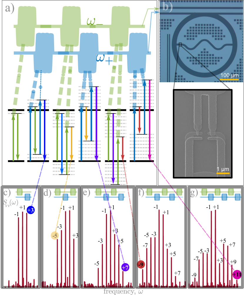
Figure 1: a) The sequence of $N$ Rabi pulses scattered on a qubit in the process of QWM. With each additional pulse, a multi-photon process with a pair of photons is emerged. This is illustrated as transitions between dressed levels shifted by $\delta\omega$ from original ones. Therefore the number of elastic peaks is increased with $N$. b) The SEM image of the transmon qubit. c)-g) The typical scattering spectra measured for $N$ from 2 to 6, respectively. The processes with $2N$ scattered photons are highlighted in color.

We prepare the input pulses with a typical heterodyne up-conversion setup with rf-sources, AWGs (arbitrary waveform generators), and IQ-mixers. As a result, two sequences of short pulses with carrier frequencies $\omega_{\pm}$ are simultaneously propagating near the qubit. Figure 1 displays an example of a sequence of 6 pulses in total. The pulse duration is typically 5-10 ns, which guarantees that the qubit keeps some coherence while interacting with every light pulse. We also introduce the gap of 2-4 ns in between pulses with different carriers, ensuring no overlap due to some parasitic reflections or rise and fall effects from AWG. This is crucial because mixing of overlapping pulses on a single two-level system gives an entirely different picture of side peaks [33]. The repetition period for each sequence is chosen to be 10 $\mu$s or more, which allows the qubit to decay freely in between the pulse sequences so that the initial state before the following pulse sequence is always the ground state with very good precision.

We down-convert the scattered light and digitize both quadratures at an intermediate frequency of 100 MHz to characterize the output field. We use high-frequency ADC with an embedded FPGA, which is programmed to average the identical traces recorded when the trigger is sent from AWG. Since we are interested here in the elastic components, the averaging time is much larger than the period of the sequence. The convenient choice is the time divisible by the period of beats with frequency $2\delta\omega$ because it allows acquiring all the temporal variations of the signal. After recording the complex average field, we make Fourier transformation to get the complex spectrum of the signal analyzed below.

The lower panels of Fig. 1 present a qualitative picture of QWM together with the measured spectra. The leftmost spectrum is obtained for the two pulses. The first pulse is at $\omega_{-}$ and the second is at $\omega_{+}$. Only one side component emerges at $\omega_{+3}$ [33]. Adding a third pulse at $\omega_{-}$ results in the appearance of two more components at $\omega_{-3}=2\omega_{-}-\omega_{+}$ and $\omega_{-5}=2\omega_{-}-\omega_{+3}=3\omega_{-}-2\omega_{+}$. The peak at $\omega_{-5}$ corresponds to the mixing of six photons, which is the highest order of mixing for three pulses. It appears when one photon is taken from the first pulse, a pair of photons from a second one, one more pair from the third one, and an extra photon is emitted at $\omega_{-5}$. With the fourth pulse at $\omega_{+}$, two more peaks appear at $\omega_{+5}$ and $\omega_{+7}$ in a similar scenario as described for three pulses. To summarize, $N$ applied pulses give rise to all processes up to $2N$-wave mixing.

To demonstrate that the observed spectral properties are controllable and may alter by time order of driving pulses, we apply three pulses: two with $\omega_{+}$ and 8 ns long and one with $\omega_{-}$ 12 ns long, see Fig. 2. The position of $\omega_{+}$ pulses is fixed, while $\omega_{-}$ pulse is moving. We start with the $\omega_{-}$ pulse being in front of two pulses at $\omega_{+}$, and finish when the pulse at $\omega_{-}$ is after two pulses at $\omega_{+}$. We observe a consistent picture of several regimes: (i) three peaks are observed when the negatively detuned pulse is either the first or the last and does not overlap with any of $\omega_{+}$ pulses; (ii) many peaks (7 or more) are observed when there is an overlap between $\omega_{+}$ and $\omega_{-}$ pulses, and (iii) five peaks when the pulses are applied one by one as depicted at the top panel of Fig 2. Therefore, the temporal configuration of driving pulses controls the qualitative properties of QWM coherent spectrum.

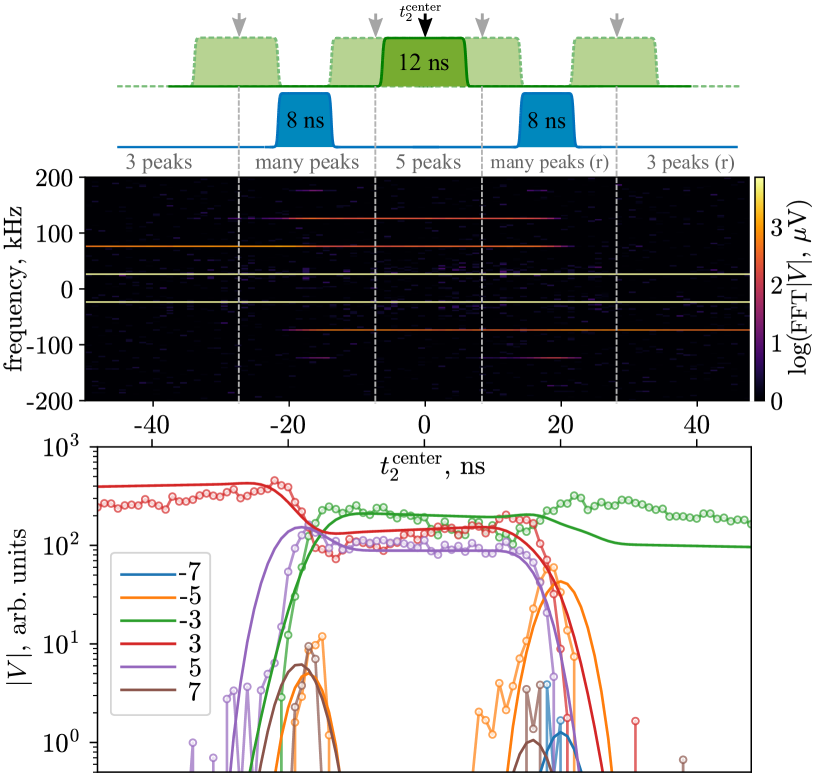
Figure 2: (upper panel) Sketch of sequence of three pulses: blue ones are with $\omega_{+}$ carrier frequency, and the green is with $\omega_{-}$. The absolute voltage of side components is plotted as a function of center position of the middle pulse $t^{\text{center}}_{2}$. The regions with specific number of components are separated by dashed vertical lines. (bottom panel) The peak amplitudes are rescaled and plotted along with the numerical simulation results.

Next, we characterize quantitative properties of side peaks. For that, we measure how durations $\Delta t_{-}$, $\Delta t_{+}$ and amplitudes $\Omega_{-}$, $\Omega_{+}$ of pulses affect the intensities of QWM components, implying that similar pulses with the same carrier frequencies rotate qubit states by equal angles. As described earlier, we make complex Fourier transformation of down-converted field, which allows us to extract amplitude and phase of any coherent component. It is also possible to rotate complex traces such that all the emitted field is concentrated in one quadrature and takes either positive or negative values. We plot color maps of these quadratures versus two arguments $\Omega_{-}\Delta t_{-}$, $\Omega_{+}\Delta t_{+}$ for each number of pulses $N$. As a result, we obtain several expressive maps demonstrating the rich dynamics of fields, see Fig. 3. We interpret the maps by explicitly calculating the evolution of the qubit under a sequence of pulses. Analytical expressions are given for each spectral component.

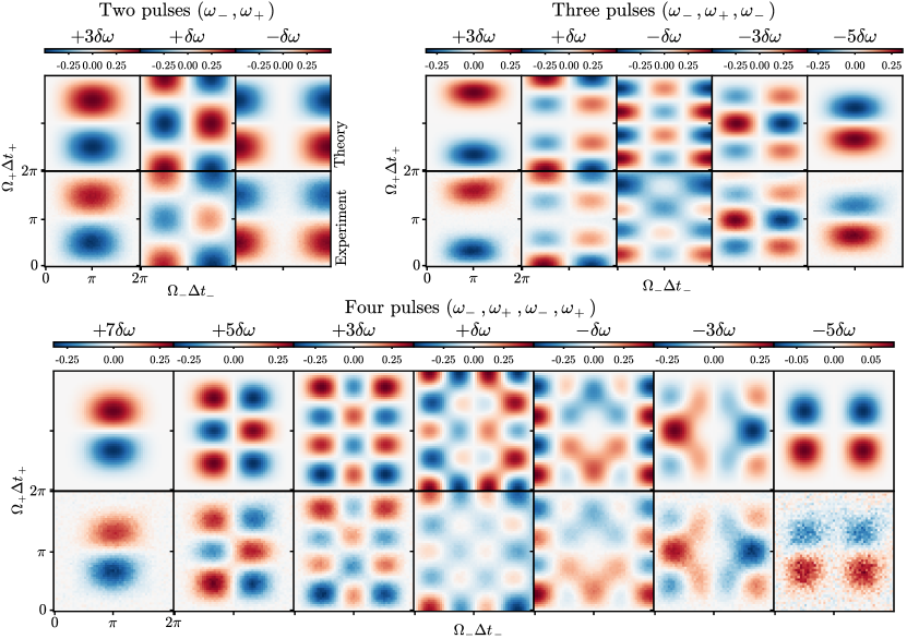
Figure 3: The heterodyne-measured complex-valued field of all observed side peaks for sequences of $N$ pulses plotted as functions of $\Omega_{+}\Delta t_{+}$ and $\Omega_{-}\Delta t_{-}$. The theoretical maps are the result of analytical calculations explained in text.

In order to interpret the observed elastic spectra in terms of multi-photon scattering, we use the framework developed in [33]. Briefly, we consider two modes of the field $c_{-},c_{+}$ with the frequencies $\omega_{+},\omega_{-}$ interacting with a qubit operators $\sigma^{-}_{\pm p}\equiv\sigma^{-}e^{\mp ip\delta t},\sigma^{+}_{\pm p}\equiv\sigma^{+}e^{\pm ip\delta t}$ which include phase acquired from coherent drive.

The Hamiltonian in the interaction picture reads

$$H=ig(c_{-}^{\dagger}\sigma^{-}_{-}-c_{-}\sigma^{+}_{-}+c_{+}^{\dagger}\sigma^{-}_{+}-c_{+}\sigma^{+}_{+}).$$ (1)

To get the field components, we first calculate the following matrix element:

$$M^{(N)}_{p}=\braket{\phi_{0}}{\Lambda_{N}^{{\dagger}}\sigma^{-}_{p}\Lambda_{N}}{\phi_{0}},$$ (2)

where the initial state is $\ket{\phi_{0}}=\ket{0,\gamma_{-},\gamma_{+}}$, meaning that the scattered field mode is initially in the ground state, and the driving fields are always in coherent states $\ket{\gamma_{-}}$ and $\ket{\gamma_{+}}$. The interaction with modes only happens when a corresponding pulse reaches the qubit. The evolution operator $\Lambda_{N}$ for $N$ applied pulses is defined as

$$\Lambda_{N}=\prod_{i=1}^{N}U_{(-1)^{i}}(\Delta t_{i}),$$ (3)

and evolution operators for every single applied pulse with the duration $\Delta t_{i}$ may approximately be expressed in the case of $\gamma_{-},\gamma_{+}\gg 1$ as

$$U_{\pm 1}\approx\cos{\frac{\theta_{\pm}}{2}}+\frac{c^{\dagger}_{\pm}\sigma^{-}_{\pm}-c_{\pm}\sigma^{+}_{\pm}}{\gamma_{\pm}}\sin{\frac{\theta_{\pm}}{2}}.$$ (4)

Here we introduced rotation angles $\theta_{\pm}=\Omega_{\pm}\Delta t_{i}$ and used $\Omega_{\pm}=2g\gamma_{\pm}$. For convenience, we also define the following operators:

$$a^{\dagger}=\alpha c_{-}\sigma^{+}_{-}/\gamma_{-},\quad b^{\dagger}=\beta c_{+}\sigma^{+}_{+}/\gamma_{+}$$ (5)

where $\alpha=\tan\theta_{-}/2$, $\beta=\tan\theta_{+}/2$.

With these expressions, for the case $N\!=\!2$, one obtains:

$$M^{(2)}_{p}=\left(\cos{\frac{\theta_{+}}{2}}\cos{\frac{\theta_{-}}{2}}\right)^{-2}\braket{\phi_{0}}{\Big{(}-\underbrace{\sigma^{-}_{p}b^{\dagger}}_{e^{i\delta t}}-\underbrace{\sigma^{-}_{p}a^{\dagger}}_{e^{-i\delta t}}+\underbrace{ab^{\dagger}\sigma^{-}_{p}a^{\dagger}}_{e^{i\delta t}}+\underbrace{ab^{\dagger}\sigma^{-}_{p}b^{\dagger}}_{e^{3i\delta t}}\Big{)}}{\phi_{0}},$$ (6)

where under brackets denote the total phase multiplier acquired from operators $a,b,a^{\dagger},b^{\dagger}$, not counting the phase of $\sigma^{-}_{p}$ for a moment. If we now calculate the time-average field at an arbitrary frequency $\omega_{p}$:

$$V^{(2)}_{p}=-i\frac{\hbar\Gamma_{1}}{\mu}\frac{1}{T}\int_{0}^{T}M^{(2)}_{p}\,dt,$$ (7)

the last term of Eq. (6) will give a non-zero component for $p\!=\!3$, since the phase multiplier from $\sigma^{-}_{+3}=\sigma^{-}e^{-3i\delta t}$ cancels out the phase picked from operators of driving modes. Therefore we see that the phases underlined in  Eq.(6) define the frequencies of non-zero elastic components observed when measuring the field spectrum with a low bandwidth. It explains the leftmost spectrum in Fig. 1 which consists of only three components. We also derive how their amplitude depends on rotation angles:

$$V^{(2)}_{3}\propto\frac{1}{2}\sin^{2}\frac{\theta_{+}}{2}\cos{\theta_{-}}$$ (8)

It is now straightforward to generalize the calculation for $N>2$ pulses. For three pulses, the analogue of Eq. (6) also expresses $M^{3}_{p}$ as a sum of terms, and among them there is only operator term $ba^{\dagger}\sigma^{-}_{p}a^{\dagger}ba^{\dagger}$ with acquired phase $e^{-5i\delta t}$, contributing to the peak at $\omega_{-5}$. This peak is highlighted on the second panel from the left in Fig. 1. For the field, we obtain

$$V^{(3)}_{-5}\propto\frac{1}{2}\sin\theta_{-}\sin^{2}\frac{\theta_{-}}{2}\sin^{2}\frac{\theta_{+}}{2}$$ (9)

The spectrum of emitted field recorded for different $\theta_{-}$ and $\theta_{+}$ allows us to reconstruct how every observable harmonic depends on rotation angles. We then compare these results with the corresponding analytical dependencies, similar to Eqs. (8) and (9). Both measured and calculated intensities are presented in Fig. 3 for $2\leq N\leq 4$. Supplemental Materials [40] contain measured results for $N=5,6$. For all measured components, the theory fits experimental maps very well, even for very high orders. Although, we notice a small disagreement for the emission at the frequency of the last pulse (either $\omega_{+}$ or $\omega_{-}$) at large effective angles. The origin of this discrepancy could be in our data processing procedure. In order to restore dependencies for $\omega_{+}$ and $\omega_{-}$, we cut out the initial pulses from the digitized traces, replacing them with zero. Therefore, a small part of the emission gets lost. Besides, some part of the last pulse might get distorted due to presence of a small impedance mismatch in the signal line. It may cause a significant effect if the rotation angle of the pulse is large.

Analyzing the patterns in Fig. 3, we can outline several specific features of the observed dependencies. First, we note that for $\theta_{-}=\theta_{+}=\pi$, all components are zero for all values of $N$. In this case, each pulse is a $\pi$-pulse; hence the qubit reaches either ground or excited state, does not contain any phase from the pulses and emits incoherently. Second, when the first pulse is negatively detuned, for all values of $N$, $\omega_{(4p-1)}$-components are zero for $\theta_{+}=\pi$, and the maps are anti-symmetrical along the line $\theta_{+}=\pi$. Similarly, the maps for $\omega_{(4p-3)}$-components are anti-symmetric relative to $\theta_{-}=\pi$ and are zero for this angle. It implies that for $\theta_{-}=\pi$ ($\theta_{+}=\pi$), there are many values of $\theta_{+}$ ($\theta_{-}$), for which emission contains only components at $\omega_{(4p-3)}$ ($\omega_{(4p-1)}$). Similar non-trivial spectral distribution was recently predicted to appear in QWM of a squeezed vacuum with a coherent field [36]. Although, here the origin of missing peaks is due to pulsed drive.

Our analytical results allow the exact identification of multi-photon contributions into every single mode. As $N$ increases, the higher-order photon processes contribute more significantly to the emission at the frequencies of initial drives and the neighboring frequencies. For example, for $N=3$, the field at $\omega_{-}$ contains only one term corresponding to a single-photon process (single-photon absorption and emission, or in analogy with higher orders, “two-wave mixing”), two terms related to the third-order processes (four-wave mixing) and one term connected with the fifth-order process (six-wave mixing). The exact expressions are presented in Supplemental Materials [40] to this article. Therefore, the interference of all these terms with different orders forms the overall pattern for every component. However, there is always only one term in the evolution responsible for the emission at the leftmost and rightmost peaks frequencies.

The observed pictures could be considered as a spectral decomposition of coherent pulses being scattered on a qubit. To illustrate the physical meaning of this decomposition, we can consider the limit $\delta\omega\rightarrow 0$. Our interleaved pulses then turn to continuous monochromatic wave exactly resonant with the qubit. The side peaks now all have the same frequency, and we can simply sum up all the contributions presented in Fig. 3 for each sequence, which results in simple Rabi dynamics, with a rotation periods corresponding to total number of pulses, see Fig. 4.

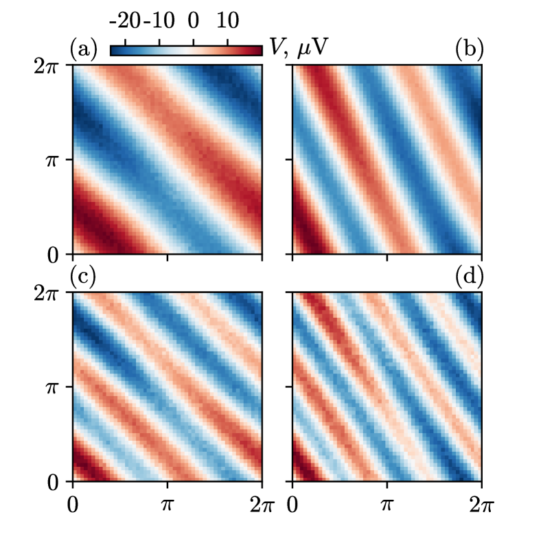
Figure 4: The net field obtained as a sum of all measured coherent components, as if it could be emitted for the drives with $\delta\omega=0$, that is, for a monochromatic drive. From (a) to (d) the map is plotted for N=2,3,4,5 pulses, horizontal axis is $\theta_{-}$ and vertical is $\theta_{+}$. The cross-sections are harmonic Rabi oscillations.

Another observation relates to the efficiency of conversion. For two applied pulses, one can see from Fig. 3a) that if $\theta_{-}=\pi$ and $\theta_{+}=\pi/2$, then all coherent field is emitted into $\omega_{+3}$ mode. We could call this point the maximal conversion point. However, note that there is also incoherently emitted radiation due to inelastic scattering. Correspondingly, for $N>2$ pulses, the distribution of coherent field among side spectral components is more complicated. Nonetheless, there are also rotation angles where the only non-zero component is $\omega_{-3}$. In summary, we study QWM of light pulses on a single qubit that reveals the intrinsic connection between qubit dynamics and allowed multi-photon processes of elastic scattering. The study of these effects will increase understanding of nonlinear quantum optics with quantum objects playing the role of a scatterer. Recent theoretical efforts show that the wave mixing of classical and quantum fields on a qubit in a waveguide is a good tool for measuring the photon statistics of the quantum signal. However, qubit itself is also a reliable source of non-classical radiation when driven continuously or by short pulses. Non-trivial coherent spectra probably indicate generation of light with more sophisticated statistics than just squeezing or antibunching. Thus, a promising area opens up for further research of microwave optics and photonics.