You Only Derive Once (YODO): Automatic Differentiation for Efficient Sensitivity Analysis in Bayesian Networks

Abstract

Sensitivity analysis measures the influence of a Bayesian network’s parameters on a quantity of interest defined by the network, such as the probability of a variable taking a specific value. In particular, the so-called sensitivity value measures the quantity of interest’s partial derivative with respect to the network’s conditional probabilities. However, finding such values in large networks with thousands of parameters can become computationally very expensive. We propose to use automatic differentiation combined with exact inference to obtain all sensitivity values in a single pass. Our method first marginalizes the whole network once using e.g. variable elimination and then backpropagates this operation to obtain the gradient with respect to all input parameters. We demonstrate our routines by ranking all parameters by importance on a Bayesian network modeling humanitarian crises and disasters, and then show the method’s efficiency by scaling it to huge networks with up to 100’000 parameters. An implementation of the methods using the popular machine learning library PyTorch is freely available.

Keywords: Automatic differentiation; Bayesian networks; Sensitivity analysis; Markov random fields; Tensor networks.

1 Introduction

Probabilistic graphical models, and specifically Bayesian networks (BNs), are a class of models that are widely used for risk assessment of complex operational systems in a variety of domains. The main reason for their success is that they provide an efficient as well as intuitive framework to represent the joint probability of a vector of variables of interest using a simple graph. Their use to assess the reliability of engineering, medical and ecological systems, among many others, is becoming increasingly popular. Sensitivity analysis is a critical step for any applied real-world analysis to assess the importance of various risk factors and to evaluate the overall safety of the system under study (see e.g. Goerlandt and Islam, 2021; Makaba et al., 2021; Zio et al., 2022, for some recent examples).

As noticed by Rohmer (2020), sensitivity analysis in BNs is usually local, in the sense that it measures the effect of a small number of parameter variations on output probabilities of interest, while other parameters are kept fixed. In the case of a single parameter variation, sensitivity analysis is usually referred to as one-way, otherwise, when more than one parameter is varied, it is called multi-way. Although recently there has been an increasing interest in proposing global sensitivity methods for BNs measuring how different factors jointly influence some function of the model’s output (see e.g. Ballester-Ripoll and Leonelli, 2022; Li and Mahadevan, 2018), the focus of this paper still lies in one-way sensitivity methods. However, extensions to multi-way local methods are readily available and discussed in Section 5.

One-way local sensitivity analysis in BNs can be broken down into two main steps. First, some parameters of the model are varied and the effect of these variations on output probabilities of interest is investigated. For this purpose, a simple mathematical function, usually termed sensitivity function, describes an output probability of interest as a function of the BN parameters (Castillo et al., 1997; Coupé and Van der Gaag, 2002). Furthermore, some specific properties of such a function can be computed, as for instance, the sensitivity value or the vertex proximity, which give an overview of how sensitive the probability of interest is to variations of the associated parameter. Such measures are reviewed below in Section 2. Second, once parameter variations are identified, the effect of these is summarized by a distance or divergence measure between the original and the varied distributions underlying the BN, most commonly the Chan-Darwiche distance (Chan and Darwiche, 2005) or the well-known Kullback-Leibler divergence.

As demonstrated by Kwisthout and van der Gaag (2008), the derivation of both the sensitivity function and its associated properties is computationally very demanding. Here we provide a novel, computationally highly-efficient method to compute all sensitivity measures of interest which takes advantage of backpropagation and is easy to compute thanks to automatic differentiation. Our algorithm is demonstrated in a BN modeling humanitarian crises and disasters (Sec. 4), and an extensive simulation study shows its efficiency by processing huge networks in a few seconds. We have open-sourced a Python implementation using the popular machine learning library PyTorch , contributing to the recent effort of promoting sensitivity analysis (Douglas-Smith et al., 2020).

2 Bayesian Networks and Sensitivity Analysis

A BN is a probabilistic graphical model defining a factorization of the probability mass function of a random vector by means of a directed acyclic graph (DAG). More formally, let $[n]=\{1,\dots,n\}$ and $\bm{Y}=(Y_{i})_{i\in[n]}$ be a random vector of interest with sample space $\mathbb{Y}=\times_{i\in[n]}\mathbb{Y}_{i}$. A BN defines the probability mass function $P(\bm{Y}=\bm{y})$, for $\bm{y}\in\mathbb{Y}$, as a product of simpler conditional probability mass functions as follows:

$$P(\bm{Y}=\bm{y})=\prod_{i\in[n]}P(Y_{i}=y_{i}\;|\;\bm{Y}_{\Pi_{i}}=\bm{y}_{\Pi_{i}}),$$ (1)

where $\bm{Y}_{\Pi_{i}}$ are the parents of $Y_{i}$ in the DAG associated to the BN.

The definition of the probability mass function over $\bm{Y}$, which would require defining $\#\mathbb{Y}-1$ probabilities, is thus simplified in terms of one-dimensional conditional probability mass functions. The coefficients of these functions are henceforth referred to as the parameters $\bm{\theta}$ of the model. The DAG structure may be either expert-elicited or learned from data using structural learning algorithms, and the associated parameters $\bm{\theta}$ can be either expert-elicited as well or learned using frequentist or Bayesian approaches. No matter the method used, we assume that a value for these parameters $\bm{\theta}$ has been chosen which we refer to as the original value and denoted as $\bm{\theta}^{0}$.

In practical applications it is fundamental to extensively assess the implications of the chosen parameter values $\bm{\theta}^{0}$ to outputs of the model. In the context of BNs this study is usually referred to as sensitivity analysis, which can actually be further used during the model building process as showcased by Coupé et al. (2000). Let $Y_{O}$ be an output variable of interest and $\bm{Y}_{E}$ be evidential variables, those that may be observed. The interest is in then studying how $P(Y_{O}=y_{O}\;|\;\bm{Y}_{E}=\bm{y}_{E})$ varies when a parameter $\theta_{i}$ is varied. In particular, $P(Y_{O}=y_{O}\;|\;\bm{Y}_{E}=\bm{y}_{E})$ seen as a function of $\theta_{i}$ is called sensitivity function and denoted as $f(\theta_{i})$.

2.1 Proportional Covariation

Notice that when an input $\theta_{i}$ is varied from its original value $\theta_{i}^{0}$ then the parameters from the same conditional probability mass function need to covary to respect the sum-to-one condition of probabilities. When variables are binary, this is automatic since one parameter must be equal to one minus the other, but for variables taking more than two levels this covariation can be done in several ways (Renooij, 2014). We henceforth assume that whenever a parameter is varied from its original value $\theta_{i}^{0}$ to a new value $\theta_{i}$, then every parameter $\theta_{j}$ from the same conditional probability mass function is proportionally covaried (Laskey, 1995) from its original value $\theta_{j}^{0}$:

$$\theta_{j}(\theta_{i})=\frac{1-\theta_{i}}{1-\theta^{0}_{i}}\theta^{0}_{j}.$$ (2)

Proportional covariation has been studied extensively and its choice is motivated by a wide array of theoretical properties (Chan and Darwiche, 2005; Leonelli et al., 2017; Leonelli and Riccomagno, 2018).

Under the assumption of proportional covariation, Castillo et al. (1997) and Coupé and Van der Gaag (2002) demonstrated that the sensitivity function is the ratio of two linear functions:

$$f(\theta_{i})=\frac{c_{1}\theta_{i}+c_{2}}{c_{3}\theta_{i}+c_{4}},$$ (3)

where $c_{1},c_{2},c_{3},c_{4}\in\mathbb{R}_{+}$. Van Der Gaag et al. (2007) noticed that the above expression actually coincides with the fragment of a rectangular hyperbola, which can be generally written as

$$f(\theta_{i})=\frac{r}{\theta_{i}-s}+t,$$ (4)

where $s=-\frac{c_{4}}{c_{3}}$, $t=\frac{c_{1}}{c_{3}}$ and $r=\frac{c_{2}}{c_{3}}+st$.

2.2 Sensitivity Value

The sensitivity value describes the effect of infinitesimally small shifts in the parameter’s original value on the probability of interest and is defined as the absolute value of the first derivative of the sensitivity function at the original value of the parameter, i.e. $|f^{{}^{\prime}}(\theta_{i}^{0})|$. This can be found by simply differentiating the sensitivity function as

$$|f^{{}^{\prime}}(\theta_{i}^{0})|=\frac{|c_{1}c_{4}-c_{2}c_{3}|}{(c_{3}\theta_{i}^{0}+c_{4})^{2}}.$$ (5)

The higher the sensitivity value, the more sensitive the output probability to small changes in the original value of the parameter. As a rule of thumb, parameters having a sensitivity value larger than one may require further investigation.

Notice that when $\bm{Y}_{E}$ is empty, i.e. the output probability of interest is a marginal probability, then the sensitivity function is linear in $\theta_{i}$ and the sensitivity value is the same no matter what the original $\theta_{i}^{0}$ was. Therefore in this case the absolute value of the gradient is sufficient to quantify the effect of a parameter to an output probability of interest.

2.3 Vertex Proximity

Van Der Gaag et al. (2007) further noticed that parameters for which the sensitivity value is small may still be such that the conditional output probability of interest is very sensitive to their variations. This happens when the original parameter value is close to the vertex of the sensitivity function, defined as the point $\theta_{i}^{v}$ at which the sensitivity value is equal to one, i.e.

$$|f^{{}^{\prime}}(\theta_{i}^{v})|=1.$$ (6)

The vertex can be derived from the equation of the sensitivity function as

$$\theta_{i}^{v}=\left\{\begin{array}[]{ll}s+\sqrt{|r|},&\mbox{if }s<0,\\ s-\sqrt{|r|},&\mbox{if }s>0.\end{array}\right.$$ (7)

Notice that the case $s=0$ is not contemplated since it would coincide to a linear sensitivity function, not an hyperbolic one.

Vertex proximity is defined as the absolute difference $|\theta_{i}^{0}-\theta_{i}^{v}|$. The smaller the vertex proximity, the more sensitive the output probabilities may be to variations of the parameter, even when the sensitivity value is small.

2.4 Other Metrics

Given the coefficients $c_{1},\dots,c_{4}$ of Eq. 3, it is straightforward to derive any property of the sensitivity function besides the sensitivity value and the vertex proximity. Here we propose the use of two additional metrics. The first is the absolute value of the second derivative of the sensitivity function at the original parameter value, which can be easily computed as:

$$|f^{\prime\prime}(\theta_{i}^{0})|=\frac{2c_{3}\left|c_{1}c_{4}-c_{2}c_{3}\right|}{\left(c_{3}\theta_{i}^{0}+c_{4}\right)^{3}}.$$ (8)

Similarly to the sensitivity value, high values of the second derivative at $\theta_{i}^{0}$ indicate parameters that could highly impact the probability of interest.

The second measure is the maximum of the first derivative of the sensitivity function over the interval $[0,1]$ in absolute value, which we find easily by noting that the denominator of Equation 5 is a parabola:

$$\max_{\theta_{i}\in[0,1]}\{|f^{\prime}(\theta_{i})|\}=\begin{cases}\infty&\mbox{ if }-c_{4}/c_{3}\in[0,1]\\ \max\{|c_{1}c_{4}-c_{2}c_{3}|/c_{4}^{2},|c_{1}c_{4}-c_{2}c_{3}|/(c_{3}+c_{4})^{2}\}&\mbox{ otherwise.}\\ \end{cases}$$ (9)

Again high values indicate parameters whose variations can lead to a significant change in the output probability of interest.

3 The YODO Method

3.1 First Case: Marginal Probability as a Function of Interest

Suppose $f(\theta_{i})=P(Y_{O}=y_{O})=c_{1}\theta_{i}+c_{2}$ assuming proportional covariation as $\theta_{i}$ moves. Let $\theta_{j_{1}},\dots,\theta_{j_{n}}$ be the other parameters of the same conditional PMF as $\theta_{i}$, i.e. they are all bound by the sum-to-one constraint $\theta_{i}+\theta_{j_{1}}+\dots+\theta_{j_{n}}=1$. First, we rewrite $f$ as

$$f(\theta_{i})=g(\theta_{i},\theta_{j_{1}}(\theta_{i}),\dots,\theta_{j_{n}}(\theta_{i}))$$ (10)

and we will show how to obtain $f^{\prime}(\theta_{i})$ provided that we can compute the gradient $\nabla g$ with respect to symbols $\theta_{i},\theta_{j_{1}},\dots,\theta_{j_{n}}$ (Sec. 3.3 for details on the latter).

By the generalized chain rule, it holds that

$$f^{\prime}(\theta_{i})=\frac{\partial g}{\partial\theta_{i}}\cdot 1+\frac{\partial g}{\partial\theta_{j_{1}}}\cdot\frac{d\theta_{j_{1}}}{d\theta_{i}}+\dots+\frac{\partial g}{\partial\theta_{j_{n}}}\cdot\frac{d\theta_{j_{n}}}{d\theta_{i}}.$$ (11)

By deriving Eq. 2, we have that for all $1\leq m\leq n$:

$$\frac{d\theta_{j_{m}}}{d\theta_{i}}=\frac{-\theta_{j_{m}}^{0}}{1-\theta_{i}^{0}}$$ (12)

and, therefore,

$$f^{\prime}(\theta_{i})=\frac{\partial g}{\partial\theta_{i}}-\frac{(\partial g/\partial\theta_{j_{1}})\cdot\theta_{j_{1}}^{0}+\dots+(\partial g/\partial\theta_{j_{n}})\cdot\theta_{j_{n}}^{0}}{1-\theta_{i}^{0}}.$$ (13)

Last, since $f(\theta_{i})=P(\bm{Y}_{O}=\bm{y}_{O})=c_{1}\theta_{i}+c_{2}$, we easily find the parameters $c_{1},c_{2}$:

$$\begin{cases}c_{1}=f^{\prime}(\theta_{i}^{0})\\ c_{2}=P(\bm{Y}_{O}=\bm{y}_{O})-c_{1}\theta_{i}^{0}.\end{cases}$$ (14)

3.2 Second Case: Conditional Probability as a Function of Interest

When $f(\theta_{i})=P(Y_{O}=y_{O}\;|\;\bm{Y}_{E}=\bm{y}_{E})=P(Y_{O}=y_{O},\bm{Y}_{E}=\bm{y}_{E})/P(\bm{Y}_{E}=\bm{y}_{E})$, we simply repeat the procedure from Sec. 3.1 twice:

1. We first apply it to $P(Y_{O}=y_{O},\bm{Y}_{E}=\bm{y}_{E})$ to obtain $c_{1}$ and $c_{2}$;

2. we then apply it to $P(\bm{Y}_{E}=\bm{y}_{E})$ to obtain $c_{3}$ and $c_{4}$.

3.3 Computing the Gradient $\nabla g$

Let $\bm{Y}_{K}=\bm{y}_{K}$ be a subset of the network variables taking some evidence values (this could be $K=O$ or $K=O\cup E$, hence we cover the two cases above).

We start by moralizing the BN into a Markov random field (MRF) $\mathcal{M}$. This marries all variable parents together and, for each conditional probability table (now called potential), drops the sum-to-one constraint; see e.g. (Darwiche, 2009) for more details. Next, we impose the evidence $\bm{Y}_{K}=\bm{y}_{K}$ by defining $\mathcal{M}^{\bm{Y}_{K}=\bm{y}_{K}}$ as a new MRF that results from substituting each potential $\Phi_{i_{1},\dots,i_{M}}(x_{i_{1}},\dots,x_{i_{M}})$ by a new potential $\widehat{\Phi}_{i_{1},\dots,i_{M}}$ defined as follows:

$$\begin{split}\widehat{\Phi}_{i_{1},\dots,i_{M}}(Y_{i_{1}}=x_{i_{1}},\dots,Y_{i_{M}}=x_{i_{M}})=\\ \begin{cases}0&\mbox{if }\exists m,k\;|\;i_{m}=k\wedge x_{i_{m}}\neq y_{i_{m}}\\ \Phi_{i_{1},\dots,i_{M}}(Y_{i_{1}}=x_{i_{1}},\dots,Y_{i_{M}}=x_{i_{M}})&\mbox{otherwise}\\ \end{cases}\end{split}$$ (15)

In other words, we copy the original potential but zero-out all entries that do not honor the assignment of values $\bm{Y}_{K}=\bm{y}_{K}$. See Tab. 1 for an example using a bivariate potential.

	$Y_{2}=1$	$Y_{2}=2$	$Y_{2}=3$
$Y_{1}=1$	0.8	0.1	0.1
$Y_{1}=2$	0.3	0.5	0.2
$Y_{1}=3$	0.1	0.2	0.7

(a) $\Phi_{1,2}(y_{1},y_{2})$

	$Y_{2}=1$	$Y_{2}=2$	$Y_{2}=3$
$Y_{1}=1$	0	0	0.1
$Y_{1}=2$	0	0	0.2
$Y_{1}=3$	0	0	0.7

(b) $\widehat{\Phi}_{1,2}(y_{1},y_{2})$

Table 1: Left: example potential of an MRF $\mathcal{M}$ for variables $Y_{1}$ and $Y_{2}$, each with three levels $\{1,2,3\}$. Right: corresponding potential for $\mathcal{M}^{Y_{2}=3}$.

Intuitively, the modified MRF $\mathcal{M}^{\bm{Y}_{K}=\bm{y}_{K}}$ represents the unnormalized probability for all variable assignments that are compatible with $\bm{Y}_{K}=\bm{y}_{K}$. In particular, if $\mathcal{M}_{\bm{Y}_{K}}$ denotes the marginalization of a network $\mathcal{M}$ over all variables in $\bm{Y}_{K}$, we have that $(\mathcal{M}^{\bm{Y}_{K}=\bm{y}_{K}})_{\bm{Y}}=P(\bm{Y}_{K}=\bm{y}_{K})$. In other words, computing $g$ reduces to marginalizing our MRF. In this paper we marginalize it exactly using the variable elimination (VE) algorithm; see e.g. (Darwiche, 2009). This method is clearly differentiable w.r.t. all parameters $\bm{\theta}$ since VE only relies on variable summation and factor multiplication. Any other differentiable inference algorithm could be used as well. This step, evaluating the function $g$, is known as the forward pass in the neural network literature. Next, we backpropagate the previous operation (a step also known as the backward pass) to build the gradient $\nabla g$. Crucially, note that backpropagation yields $\partial g/\partial\theta$ for every parameter $\theta\in\bm{\theta}$ of the network at once, not just an individual $\theta_{i}$. Last, we obtain parameters $c_{1},\dots,c_{4}$ as detailed before, and use them to compute the metrics of Secs. 2.2, 2.3, and 2.4 for each $\theta_{i}$.

Note the advantages of this approach as compared to other alternatives. For example, symbolically deriving the gradient of $g$ would be cumbersome and would depend on the target network topology and definition of the probability of interest (Darwiche, 2003). Automatic differentiation avoids this by evaluating the gradient numerically using the chain rule. Furthermore, finding the gradient using finite differences would require evaluating $g$ twice per parameter $\theta_{i}$. In contrast, automatic differentiation only requires a forward and backward pass to find the entire gradient –in our experiments, this took roughly the time of just two marginalization operations (see next section).

4 Results

We overview first the insights revealed by our method when applied on a 21-node Bayesian network of interest; we then study the method’s scalability by testing it on large networks with hundreds of nodes and arcs and up to $10^{5}$ parameters.

4.1 Software and Hardware Used

In order to perform variable elimination efficiently, we note that the problem of graphical model marginalization is equivalent to that of tensor network contraction Robeva and Seigal (2018), and use the library opt_einsum Smith and Gray (2018) which offers optimized heuristics for the latter. As backend we use the state-of-the-art machine learning library PyTorch Paszke et al. (2019), version 1.11.0, to do all operations between tensors and then perform backpropagation on them. We use pgmpy (Ankan and Panda, 2015) for reading and moralizing BNs.

All experiments were run on a 4-core i5-6600 3.3GHz Intel workstation with 16GB RAM.

4.2 Risk Assessment for Humanitarian Crises and Disasters

Similarly to Qazi and Simsekler (2021), we construct a BN model to assess the country-level risk associated with humanitarian crises and disasters. The data was collected from INFORM (INFORM, 2022) and consists of 20 drivers of disaster risk covering natural, human, socio-economic, institutional and infrastructure factors that influence the country-level risk of a disaster, together with a final country risk index which summarizes how exposed a country is to the possibility of a humanitarian disaster. A full list of the variables can be found at INFORM (2022). All variables take values between zero and ten and have been discretized into three categories (low/0, medium/1, high/2) using the equal-length method. The dataset comprises 190 countries.

A BN is learned using the hc function of the bnlearn package and is reported in Figure 1. As an illustration of the YODO method, we compute here all sensitivity measures for the conditional probability of a high disaster risk (RISK = 2) conditional on a high risk of flooding (FLOOD = 2). Computing all metrics for all 183 network parameters with our method took only 0.055 seconds. The results are reported in Table 2 for the 20 most influential parameters according to the sensitivity value. It can be noticed that the most influential parameters come from the conditional distributions of the overall risk given the development and deprivation index (D_AND_D), as well as from the conditional distribution of the flooding index given a projected conflict risk index (PCR) equal to low. As an additional illustration, Figure 2 reports the sensitivity value of the parameters for the output conditional probability of a high risk given a high risk of earthquake. The blue color is associated to positive values of the sensitivity value, the red color for negative ones. Out of 183 network parameters, 30 had a sensitivity value of zero, meaning that they had no effect on the probability of interest.

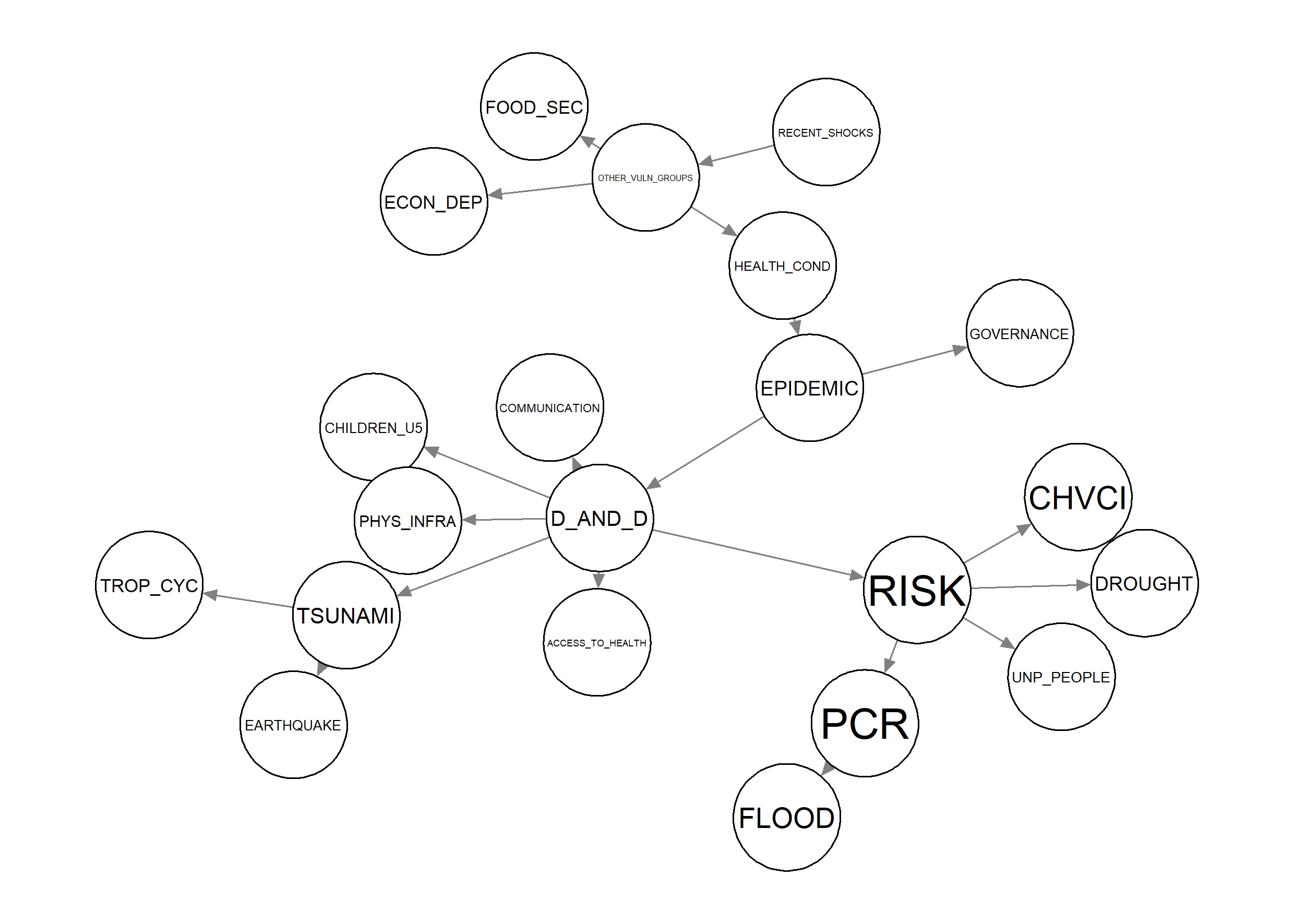
Figure 1: BN learned over the INFORM (2022) dataset for country-level disaster risk.

	Value	Sens. value	Proximity	$2^{\mbox{nd}}$ deriv.	Largest $1^{\mbox{st}}$ deriv.
Parameter
RISK = high $|$ D_AND_D = low	$0.0012$	$0.914$	$0.056$	$-1.437$	$0.916$
FLOOD = high $|$ PCR = low	$0.107$	$0.722$	$0.0534$	$4.059$	$1.475$
FLOOD = medium $|$ PCR = low	$0.469$	$0.645$	$0.718$	$3.238$	$\infty$
FLOOD = low $|$ PCR = low	$0.425$	$0.645$	$0.718$	$3.238$	$\infty$
RISK = high $|$ D_AND_D = high	$0.34$	$0.555$	$0.731$	$-0.387$	$0.714$
RISK = high $|$ D_AND_D = medium	$0.0686$	$0.467$	$1.002$	$-0.295$	$0.488$
EPIDEMIC = high $|$ HEALTH_COND = low	$0.148$	$0.295$	$1.167$	$-0.231$	$0.332$
D_AND_D = high $|$ EPIDEMIC = medium	$0.0742$	$0.238$	$1.834$	$-0.133$	$0.249$
PCR = high $|$ RISK = medium	$0.278$	$0.226$	$0.6$	$0.395$	$0.394$
PCR = high $|$ RISK = low	$0.0266$	$0.204$	$0.694$	$0.322$	$0.213$
FLOOD = high $|$ PCR = high	$0.509$	$0.196$	$0.475$	$-0.46$	$1.211$
FLOOD = high $|$ PCR = medium	$0.136$	$0.167$	$0.787$	$0.25$	$0.206$
D_AND_D = high $|$ EPIDEMIC = high	$0.787$	$0.159$	$4.159$	$-0.0459$	$0.202$
D_AND_D = high $|$ EPIDEMIC = low	$0.0411$	$0.153$	$2.984$	$-0.0625$	$0.156$
RISK = low $|$ D_AND_D = high	$0.0208$	$0.151$	$2.319$	$-0.0796$	$0.274$
HEALTH_COND = medium $|$ OTHER_VULN_GROUPS = low	$0.05$	$0.151$	$3.026$	$-0.061$	$0.154$
HEALTH_COND = low $|$ OTHER_VULN_GROUPS = low	$0.949$	$0.15$	$3.036$	$-0.0606$	$0.154$
PCR = low $|$ RISK = high	$0.00521$	$0.15$	$3.023$	$-0.0609$	$0.236$
D_AND_D = medium $|$ EPIDEMIC = high	$0.176$	$0.148$	$5.393$	$-0.0338$	$0.18$
PCR = high $|$ RISK = high	$0.943$	$0.148$	$3.092$	$-0.0588$	$0.224$
PCR = medium $|$ RISK = high	$0.0521$	$0.146$	$3.144$	$-0.0573$	$0.22$
D_AND_D = low $|$ EPIDEMIC = high	$0.0368$	$0.144$	$2.859$	$-0.0626$	$0.231$
FLOOD = low $|$ PCR = medium	$0.103$	$0.144$	$0.955$	$0.187$	$0.165$
FLOOD = medium $|$ PCR = medium	$0.762$	$0.144$	$0.955$	$0.187$	$0.565$
RISK = medium $|$ D_AND_D = high	$0.64$	$0.137$	$1.99$	$-0.0869$	$0.175$
PCR = low $|$ RISK = medium	$0.422$	$0.12$	$1.399$	$0.112$	$0.226$
HEALTH_COND = high $|$ OTHER_VULN_GROUPS = low	$9.083\cdot 10^{-4}$	$0.113$	$4.302$	$-0.0348$	$0.113$
OTHER_VULN_GROUPS = low $|$ RECENT_SHOCKS = low	$0.82$	$0.112$	$4.418$	$-0.0337$	$0.118$
OTHER_VULN_GROUPS = medium $|$ RECENT_SHOCKS = low	$0.173$	$0.111$	$4.454$	$-0.0333$	$0.117$
PCR = low $|$ RISK = low	$0.947$	$0.109$	$1.578$	$0.0928$	$0.115$

Table 2: Four sensitivity metrics for the top 30 parameters of the humanitarian crisis network (ranked by their sensitivity value), when the probability of interest is $P(\mbox{RISK}=\mbox{high}\;|\;\mbox{FLOOD}=\mbox{high})$.

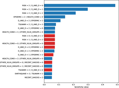
Figure 2: Top 20 most influential parameters for the humanitarian crisis network, color-coded by the sign of $f^{\prime}(\theta_{i})$. The probability of interest is $P(\mbox{RISK}=\mbox{high}\;|\;\mbox{EARTHQUAKE}=\mbox{high})$.

4.3 Performance Study over Medium to Very Large Networks

We further run our method over the 10 Bayesian networks considered in Scutari et al. (2019). As a baseline we use numerical estimation of each sensitivity value via finite differences, whereby we slightly perturb each parameter $\theta_{i}$ and measure the impact on $f$. As a probability of interest we set $P(A=a|B=b)$, where $A,B,a,b$ were two variables and two levels picked at random, respectively, and each timing is the average of three independent runs. Results are reported in Table 3, which shows that YODO outperforms the baseline by several orders of magnitude.

	#nodes	#arcs	#parameters	Treewidth	Time (fin. diff.)	Time (ours)
Network
child	20	30	344	3	2.188733	0.017727
water	32	123	13484	10	337.189158	0.054150
alarm	37	65	752	4	10.203079	0.034412
hailfinder	56	99	3741	4	98.040870	0.053667
hepar2	70	158	2139	6	169.150984	0.093187
win95pts	76	225	1148	8	38.674632	0.113214
pathfinder	109	208	97851	6	8596.810546	0.188448
munin1	186	354	19226	11	113928.398017	14.394249
andes	223	626	2314	17	252.286060	0.299587
pigs	441	806	8427	10	3213.308629	0.521486

Table 3: Our method was applied to 10 Bayesian networks, here sorted by number of nodes. All times are in seconds. The times for the baseline (second-to-last column) were estimated as the total number of parameters in the network times the time needed to numerically estimate one sensitivity value. Treewidths were found with the NetworkX graph library Hagberg et al. (2008).

5 Discussion

We demonstrated the use of automatic differentiation in the area of BNs and more specifically in the study of how sensitive they are to variations of their parameters. The novel algorithms are freely available in Python and are planned to be included in the next release of the bnmonitor R package (Leonelli et al., 2021). Their efficiency was demonstrated through a simulation study and their use in practice was illustrated through a BN in the field of risk assesment for humanitarian crises.

Although YODO is specifically designed to compute the coefficients of the sensitivity function in Equation 3, it further addresses two additional problems in sensitivity analysis. First, it is able to quickly find which parameters do have an effect on the output probability of interest, which is usually called the parameter sensitivity set (Coupé and Van der Gaag, 2002). Second, we identify whether a parameter change leads to a monotonically increasing or decreasing sensitivity function, as already addressed in Bolt and Renooij (2017). Although the above-cited works only require the structure of the network, YODO yields an efficient way to tackle the same problems.

Future Work

Because of the space constraint we only focused on one-way sensitivity analysis but, because of their efficiency, the proposed methods could be generalized to multi-way sensitivity analysis where more than one parameter is varied contemporaneously. Bolt and Renooij (2014) introduced the maximum/minimum n-way sensitivity value which bounds the effect of n-way variations of parameters and demonstrated that it can be easily derived from the sensitivity values of one-way sensitivity analyses. Therefore, our methods could be extended to also efficiently compute the joint effect of variations of parameters, known to be computationally challenging (Chan and Darwiche, 2004; Kjaerulff and van der Gaag, 2000).

Another possible extension of the algorithms introduced here would be to compute the so-called admissible deviation (van der Gaag and Renooij, 2001). This consists of finding a pair of numbers $(\alpha,\beta)$ that describe the shifts to smaller values and to larger values, respectively, that are allowed in the parameter under study without inducing a change in the most likely value of the output variable. For a parameter with an original value of $\theta_{i}^{0}$, the admissible deviation $(\alpha,\beta)$ thus indicates that the parameter can be safely varied within the interval $(\theta_{i}^{0}-\alpha,\theta_{i}^{0}+\beta)$. These values can be straightforwardly found by identifying the intersections of the sensitivity functions associated to different values of the output variable.

References

- Ankan and Panda (2015) A. Ankan and A. Panda. pgmpy: Probabilistic graphical models using python. In Proceedings of the 14th Python in Science Conference (SCIPY 2015). Citeseer, 2015.
- Ballester-Ripoll and Leonelli (2022) R. Ballester-Ripoll and M. Leonelli. Computing Sobol indices in probabilistic graphical models. Reliability Engineering & System Safety, 225:108573, 2022.
- Bolt and Renooij (2014) J. H. Bolt and S. Renooij. Local sensitivity of Bayesian networks to multiple simultaneous parameter shifts. In European Workshop on Probabilistic Graphical Models, pages 65–80, 2014.
- Bolt and Renooij (2017) J. H. Bolt and S. Renooij. Structure-based categorisation of Bayesian network parameters. In European Conference on Symbolic and Quantitative Approaches to Reasoning and Uncertainty, pages 83–92, 2017.
- Castillo et al. (1997) E. Castillo, J. M. Gutiérrez, and A. S. Hadi. Sensitivity analysis in discrete Bayesian networks. IEEE Transactions on Systems, Man, and Cybernetics-Part A: Systems and Humans, 27(4):412–423, 1997.
- Chan and Darwiche (2004) H. Chan and A. Darwiche. Sensitivity analysis in Bayesian networks: From single to multiple parameters. In Proceedings of the 20th UAI Conference, pages 67–75, 2004.
- Chan and Darwiche (2005) H. Chan and A. Darwiche. A distance measure for bounding probabilistic belief change. International Journal of Approximate Reasoning, 38(2):149–174, 2005.
- Coupé and Van der Gaag (2002) V. M. Coupé and L. C. Van der Gaag. Properties of sensitivity analysis of Bayesian belief networks. Annals of Mathematics and Artificial Intelligence, 36(4):323–356, 2002.
- Coupé et al. (2000) V. M. Coupé, L. C. Van Der Gaag, and J. D. F. Habbema. Sensitivity analysis: an aid for belief-network quantification. The Knowledge Engineering Review, 15(3):215–232, 2000.
- Darwiche (2003) A. Darwiche. A differential approach to inference in Bayesian networks. Journal of the ACM (JACM), 50(3):280–305, 2003.
- Darwiche (2009) A. Darwiche. Modeling and reasoning with Bayesian networks. Cambridge University Press, 2009.
- Douglas-Smith et al. (2020) D. Douglas-Smith, T. Iwanaga, B. F. Croke, and A. J. Jakeman. Certain trends in uncertainty and sensitivity analysis: An overview of software tools and techniques. Environmental Modelling & Software, 124:104588, 2020.
- Goerlandt and Islam (2021) F. Goerlandt and S. Islam. A Bayesian Network risk model for estimating coastal maritime transportation delays following an earthquake in British Columbia. Reliability Engineering & System Safety, 214:107708, 2021.
- Hagberg et al. (2008) A. A. Hagberg, D. A. Schult, and P. J. Swart. Exploring network structure, dynamics, and function using NetworkX. In Proceedings of the 7th Python in Science Conference, pages 11–15, 2008.
- INFORM (2022) INFORM. Index for risk management. Retrieved from https://drmkc.jrc.ec.europa.eu/inform-index, 2022.
- Kjaerulff and van der Gaag (2000) U. Kjaerulff and L. van der Gaag. Making sensitivity analysis computationally efficient. In Proceedings of the 17th UAI Conference, pages 317–325, 2000.
- Kwisthout and van der Gaag (2008) J. Kwisthout and L. van der Gaag. The computational complexity of sensitivity analysis and parameter tuning. In Proceedings of the 24th UAI Conference, pages 349–356, 2008.
- Laskey (1995) K. B. Laskey. Sensitivity analysis for probability assessments in Bayesian networks. IEEE Transactions on Systems, Man, and Cybernetics, 25(6):901–909, 1995.
- Leonelli and Riccomagno (2018) M. Leonelli and E. Riccomagno. A geometric characterisation of sensitivity analysis in monomial models. arXiv:1901.02058, 2018.
- Leonelli et al. (2017) M. Leonelli, C. Görgen, and J. Q. Smith. Sensitivity analysis in multilinear probabilistic models. Information Sciences, 411:84–97, 2017.
- Leonelli et al. (2021) M. Leonelli, R. Ramanathan, and R. L. Wilkerson. Sensitivity and robustness analysis in Bayesian networks with the bnmonitor R package. arXiv:2107.11785, 2021.
- Li and Mahadevan (2018) C. Li and S. Mahadevan. Sensitivity analysis of a Bayesian network. ASCE-ASME J Risk and Uncert in Engrg Sys Part B Mech Engrg, 4(1), 2018.
- Makaba et al. (2021) T. Makaba, W. Doorsamy, and B. S. Paul. Bayesian network-based framework for cost-implication assessment of road traffic collisions. International journal of intelligent transportation systems research, 19(1):240–253, 2021.
- Paszke et al. (2019) A. Paszke, S. Gross, F. Massa, and et al. PyTorch: An imperative style, high-performance deep learning library. In H. Wallach, H. Larochelle, A. Beygelzimer, F. d'Alché-Buc, E. Fox, and R. Garnett, editors, Advances in Neural Information Processing Systems, pages 8024–8035. Curran Associates, Inc., 2019.
- Qazi and Simsekler (2021) A. Qazi and M. C. E. Simsekler. Assessment of humanitarian crises and disaster risk exposure using data-driven Bayesian networks. International Journal of Disaster Risk Reduction, 52:101938, 2021.
- Renooij (2014) S. Renooij. Co-variation for sensitivity analysis in Bayesian networks: properties, consequences and alternatives. International Journal of Approximate Reasoning, 55(4):1022–1042, 2014.
- Robeva and Seigal (2018) E. Robeva and A. Seigal. Duality of graphical models and tensor networks. Information and Inference: A Journal of the IMA, 8(2):273–288, 06 2018.
- Rohmer (2020) J. Rohmer. Uncertainties in conditional probability tables of discrete Bayesian belief networks: A comprehensive review. Engineering Applications of Artificial Intelligence, 88:103384, 2020.
- Scutari et al. (2019) M. Scutari, C. E. Graafland, and J. M. Gutiérrez. Who learns better Bayesian network structures: Accuracy and speed of structure learning algorithms. International Journal of Approximate Reasoning, 115:235–253, 2019.
- Smith and Gray (2018) D. G. A. Smith and J. Gray. opt_einsum - a Python package for optimizing contraction order for einsum-like expressions. Journal of Open Source Software, 3(26):753, 2018.
- van der Gaag and Renooij (2001) L. van der Gaag and S. Renooij. Analysing sensitivity data from probabilistic networks. In Proceedings of the 18th UAI Conference, pages 530–537, 2001.
- Van Der Gaag et al. (2007) L. C. Van Der Gaag, S. Renooij, and V. M. Coupé. Sensitivity analysis of probabilistic networks. In Advances in probabilistic graphical models, pages 103–124. Springer, 2007.
- Zio et al. (2022) E. Zio, M. Mustafayeva, and A. Montanaro. A Bayesian belief network model for the risk assessment and management of premature screen-out during hydraulic fracturing. Reliability Engineering & System Safety, 218:108094, 2022.