A Deep Learning Approach for the Segmentation of
Electroencephalography Data in Eye Tracking Applications

Abstract

The collection of eye gaze information provides a window into many critical aspects of human cognition, health and behaviour. Additionally, many neuroscientific studies complement the behavioural information gained from eye tracking with the high temporal resolution and neurophysiological markers provided by electroencephalography (EEG). One of the essential eye-tracking software processing steps is the segmentation of the continuous data stream into events relevant to eye-tracking applications, such as saccades, fixations, and blinks. Here, we introduce DETRtime, a novel framework for time-series segmentation that creates ocular event detectors that do not require additionally recorded eye-tracking modality and rely solely on EEG data. Our end-to-end deep-learning-based framework brings recent advances in Computer Vision to the forefront of the times series segmentation of EEG data. DETRtime achieves state-of-the-art performance in ocular event detection across diverse eye-tracking experiment paradigms. In addition to that, we provide evidence that our model generalizes well in the task of EEG sleep stage segmentation.

1 Introduction and Motivation

Eye gaze information is widely used in cognitive neuroscience and psychology. Moreover, many neuroscientific studies complement scientific methods such as functional magnetic resonance imaging (fMRI) and electroencephalography (EEG) with eye-tracking technology to identify variations in attention, arousal, and the participant’s compliance with the task demands (Hanke et al., 2019). This way, the combined EEG and eye-tracking studies can provide an “ideal neuroscience model” to investigate brain-behaviour associations (Luna et al., 2008). Nowadays, infrared video-based eye trackers are the most common approach in scientific studies. Although costs for infrared video-based are slowly becoming less prohibitive, these devices remain outside the range of access for many researchers due to the added layers of complexity (e.g., operator training, setup time, synchronization of eye-tracking data with fMRI or EEG, and analysis of an additional data type) that can be burdensome (Holmqvist et al., 2011). In addition, once installed, setup and calibration for each scanning session also can be time-consuming (Fuhl et al., 2016).
Nonetheless, recent evidence (Kastrati et al., 2021c, a) suggests that gaze position can be computed by using the combination of EEG and deep learning. Our benchmark and a dataset for estimation of gaze position intending to simulate a purely EEG-based eye-tracker shows that this task is challenging to solve with high accuracy.
However, even the segmentation of continuous EEG data stream into ocular events (i.e. fixations, saccades and blinks), the prerequisite for an EEG based eye-tracker, can provide meaningful insights into human behaviour (Toivanen et al., 2015). For instance, blinks can indicate various human states, including fatigue or drowsiness (Schmidt et al., 2018). Moreover, the analysis of the gaze activity recognition allows us to study changes in cognitive workload (Buettner, 2013), recognize the context from gaze pattern behaviour (Bulling & Roggen, 2011), and even detect microsleep episodes in eye movement data while driving a car (Behrens et al., 2010). Despite these benefits, no deep-learning based approach that segments the EEG signal into meaningful ocular events is available in daily research and clinical practice.
To address this shortcoming, we developed the first neural network-based segmentation method to identify and differentiate ocular events from continuous EEG data. In this paper, we introduce DETRtime, a novel time series network architecture that can be used for the segmentation of events in a unified manner. The DETRtime is based on the DETR architecture (Carion et al., 2020b) that was initially proposed for object detection.
Our time series adaptation maps sequential inputs of arbitrary length to sequences of class labels on a freely chosen temporal scale. We evaluated DETRtime on EEG data consisting of recordings from 4 experimental paradigms and overall 168 participants. In addition, we provided evidence on a second task, namely EEG sleep stage segmentation. For that matter, we ran experiments on the publicly available Sleep-EDF-153 dataset (Goldberger AL, 2000).

In all cases, we found that DETRtime outperforms current state-of-the-art deep learning models on both the ocular event and sleep stage segmentation.
To conclude, our main contributions are:

• A novel, purely EEG-based segmentation technique for eye-tracking applications.

• An adaption of the Detection Transformer (DETR) architecture (Carion et al., 2020b), introducing instance segmentation to the analysis of EEG data and providing a performant alternative to the current state-of-the-art which implements (often convolution-based) semantic segmentation (Thoma, 2016).

• A collection of two novel ocular event datasets (Movie Watching and Large Grid paradigm) containing 139k fixations, 139k saccades and 14k blinks, with concurrently recorded EEG and infrared video-based eye-tracking serving as ground truth.

2 Related Work

The ocular events’ detection is an active research topic with applications in human behaviour analysis (Mele & Federici, 2012), activity recognition (Bulling & Roggen, 2011), human-computer interaction and usability research (Jacob & Karn, 2003), to mention a few.
The most standard and exploited segmentation techniques rely on infrared video-based systems. Modern eye-tracker companies use proprietary solutions to enable fast and reliable data segmentation (Engbert & Kliegl, 2003; Nyström & Holmqvist, 2010). These approaches utilize adaptive thresholds freeing researchers from setting different thresholds per trial when the noise level varies between trials. Another notable example of the segmentation framework was provided by (Zemblys et al., 2018). This deep learning-based solution detects eye movements from eye-tracking data and does not require hand-crafted signal features or signal thresholding. However, in many experimental settings, a camera setup for eye tracking is not available, and thus this approach becomes impossible.
Another technique of measuring eye movements is Electrooculography (EOG), which records changes in electric potentials that originate from movements of the eye muscles (Barea et al., 2002). Previous studies have described and evaluated algorithms for detecting saccade, fixation, and blink characteristics from EOG signals recorded while driving a car (Behrens et al., 2010). The proposed algorithm detects microsleep episodes in eye movement data, showing the high importance of the tool. Other authors (Bulling et al., 2009) have successfully evaluated algorithms for detecting three eye movement types from EOG signal achieving average precision of 76.1 % and recall of 70.5 % over all classes and participants. To date, the most successful and comprehensive approach to the problem of the EOG segmentation was proposed by (Pettersson et al., 2013). They classified temporal eye parameters (saccades, blinks) from EOG data. The classification sensitivity for horizontal and large saccades was larger than 89% and for vertical saccades larger than 82%. Another line of research on the subject has been mostly restricted to blink detection (Kleifges et al., 2017). Their BLINKER algorithm effectively captures most of the blinks and calculates common ocular indices. Nonetheless, to the best of our knowledge, an end-to-end continuous EEG data stream segmentation framework for eye-tracking applications is missing. One of the prominent attempts for EEG data segmentation applied to sleep staging was targeted in (Perslev et al., 2019). The proposed architecture, U-Time, could learn sleep staging based on various input channels across healthy and diseased subjects, obtaining a global F1 score above 0.75. However, the authors did not address the problem of segmenting the continuous EEG data stream into ocular events. Nevertheless, they recommended their network architecture as a universal tool for the segmentation of various psychophysiological datasets (Perslev et al., 2019). Recent improvements in sleep staging research were obtained by the introduction of SalientSleepNet (Jia et al., 2021). The proposed fully convolutional network is based on the $U^{2}$-Net architecture, originally proposed for salient object detection in computer vision. SalientSleepNet shows performance improvements over U-Time on the publicly available Sleep-EDF-39, and Sleep-EDF-153 datasets (Goldberger AL, 2000). Thus, we apply both U-Time and SalientSleepNet as part of our baseline efforts.

3 Experimental Setup and Dataset

The experiment took place in a sound-attenuated and darkened room. The participant was seated at a distance of 68cm from a 24-inch monitor (ASUS ROG, Swift PG248Q, display dimensions 531×299 mm, resolution 800×600 pixels resulting in a display: 400×298.9 mm, vertical refresh rate of 100Hz). Participants completed the tasks sitting alone, while research assistants monitored their progress in the adjoining room. The study was approved by the local ethics commission.

3.1 Data Acquisition

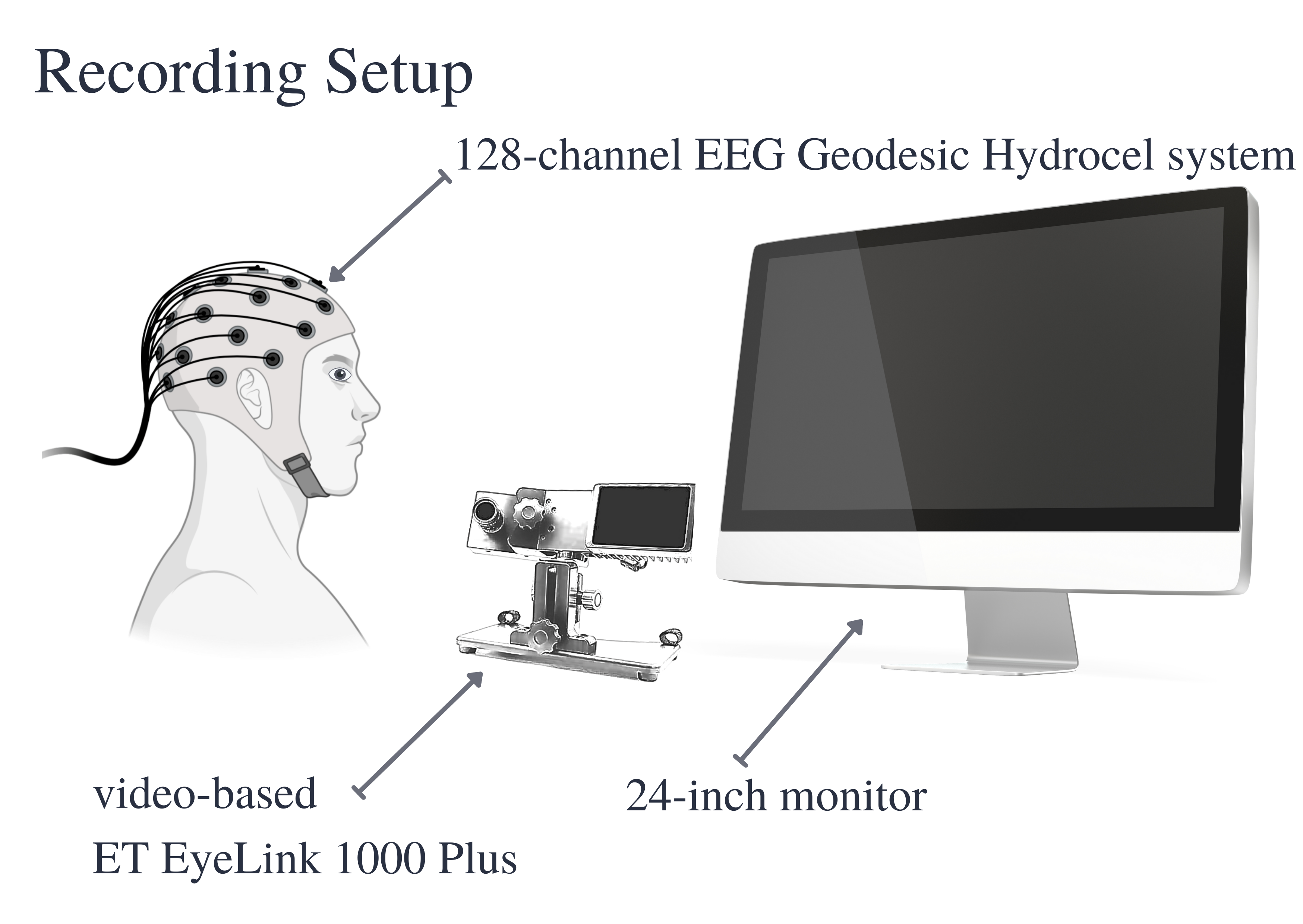
Figure 1: The illustration of the recording setup

Participants

We collected data from 168 healthy adults (age range 20-80 years, 92 females) across four experimental paradigms (see Section 3.2). All participants gave written consent for their participation and the re-use of the data prior to the start of the experiments. All participants received a monetary compensation (the local currency equivalent of 25 United States Dollars) per hour of the engagement.

Eye-Tracking Acquisition

Eye movements were recorded with an infrared video-based eye tracker (EyeLink 1000 Plus, SR Research) at a sampling rate of 500 Hz and an instrumental spatial resolution of 0.01°. The eye-tracker was calibrated with a 9-point grid at the beginning of the session and re-validated before each block of trials. Participants were instructed to keep their gaze on a given point until it disappeared. If the average error of all points (calibration vs. validation) was below 1° of visual angle, the positions were accepted. Otherwise, the calibration was redone until this threshold was reached.

EEG Acquisition

We recorded the high-density EEG data at a sampling rate of 500 Hz with a bandpass of 0.1 to 100 Hz, using a 128-channel EEG Geodesic Hydrocel system. A signal snippet can be seen in Figure 3. The Cz electrode served as a recording reference. The impedance of each electrode was checked before recording and was kept below 40 $k\Omega$. Additionally, electrode impedance levels were checked approximately every 30 minutes and reduced if necessary.

3.2 Stimuli & Experimental Design

Figure 2: Schematic overview of all experimental paradigms used in our evaluation: Movie Watching, Natural Reading, Visual Symbol Search, and Large Grid.

Large Grid

We used the Large Grid paradigm as proposed in (Kastrati et al., 2021a), where participants fixate on a series of sequentially presented dots, each at one of 25 unique positions (presentation duration = 1.5-1.8s). This experimental paradigm is similar to the calibration procedures, which are used in infrared video- based eye-tracking approaches. The positions cover all corners of the screen as well as the center (see Figure 2). Unlike the others, the dot at the center of the screen appears three times, resulting in 27 trials (displayed dots) per block. To record a larger number of trials and reduce the predictability of the subsequent positions in the primary sequence of the stimulus, we used different pseudo-randomized orderings of the dots presentation, distributed in five experimental blocks, as shown in Figure 3. The entire procedure was repeated 6 times during the measurement, resulting in 810 stimuli presentations per each participant.

Visual Symbol Search

Visual Symbol Search (VSS) paradigm is a computerized version of a clinical assessment to measure processing speed (Symbol Search Subtest of the Wechsler Intelligence Scale for Children IV (WISC-IV) (Wechsler & Kodama, 1949)) and the Wechsler Adult Intelligence Scale (WAIS-III)  (Wechsler, 1955)). Participants are shown 15 rows at a time, where each row consists of two target symbols, five search symbols and two additional symbols that contain respectively the words “YES” and “NO”. For each row, participants need to indicate by clicking with the mouse button on the “YES” or “NO” symbol, whether or not one of the two target symbols appears among the five search symbols (Kastrati et al., 2021b). A schematic overview can be found in Figure 2. For detailed event information of the dataset we refer to Appendix G.3.

Natural Reading

In order further explore performance under natural viewing conditions, we test our model suite on the publicly available ZuCo 2.0 dataset (Hollenstein et al., 2019). ZuCo 2.0 is a dataset containing simultaneous eye-tracking and electroencephalography data collected during natural reading. The dataset we use contains gaze and brain activity data from nine participants reading English language sentences, both in a normal reading paradigm and in a task-specific paradigm. In the latter, participants actively search for a semantic relation type in the given sentences as a linguistic annotation task. A schematic overview of the experimental paradigm can be found in Figure 2. For detailed event information we refer to Appendix G.2.

Movie Watching

The Movie Watching paradigm enables the collection of EEG data in a naturalistic viewing setting. Data were obtained during two short and highly engaging movies scenes (‘Despicable Me’ [171 seconds clip, MPEG-4 movie, the bedtime ("Three Little Kittens") scene] and ‘Fun Fractals’ [163 seconds clip, MPEG-4 movie]). A schematic view of the experimental paradigm can be found in Figure 2. For detailed event information we refer to Appendix G.1.

3.3 Preprocessing and Data Annotation

Eye-Tracking Preprocessing

Existing literature studying eye movement generally distinguishes between three different ocular events (Toivanen et al., 2015): saccades, fixations, and blinks. Saccades are rapid, ballistic eye movements that instantly change the gaze position. Saccade onsets are detected using the eye-tracking software default settings: acceleration larger than 8000°/s², a velocity above 30°/s, and a deflection above 0.1°. Fixations are defined as time periods while maintaining of the gaze on a single location (Engbert & Kliegl, 2003), and blinks are considered a special case of fixation, where the pupil diameter is zero. One example of such labeled data is shown in Figure 3.

Electroencephalography Preprocessing

EEG data is often contaminated by artifacts produced by environmental factors, e.g., temperature, air humidity, as well as other sources of electromagnetic noise, such as line noise (Kappenman & Luck, 2010) and therefore requires preprocessing in the form of artifact cleaning or artifact correction (Keil et al., 2014). Our EEG preprocessing included detecting and interpolating bad electrodes and filtering the data with a 0.1 Hz high-pass filter. With this “minimal” preprocessing pipeline, the preprocessed data still retains ocular activity, which can be used to infer the ocular events (the signal of interest in the present study). The detailed preprocessing pipeline is described in Appendix F.

EEG & Eye-Tracking Synchronization

In the next step, the EEG and eye-tracking data were synchronized using the EYE-EEG toolbox (Dimigen et al., 2011) to enable EEG analyses time-locked to the onsets of fixations and saccades, and subsequently segment the EEG data based on the eye-tracking measures. The synchronization algorithm first identified the “shared” events between eye-tracking and electroencephalography recordings (start end trigger of each experimental paradigm). Next, a linear function was fitted to the shared event latencies to refine the start- and end-event latency estimation in the eye tracker recording. Finally, the synchronization quality was ensured by comparing the trigger latencies recorded in the EEG and eye-tracker data. As a result, all synchronization errors did not exceed 2 ms (i.e., one data point).

4 EEG Segmentation Task & Metric

For each of the four datasets we approached the task of segmenting the EEG data into three different ocular events: fixations, saccades and blinks. As illustrated in Figure 3, the goal of this task was to classify each time point (i.e 2ms) of the 128-channel EEG stream of data as a unique event.

Data Structure

Since our model operates on samples of arbitrary length (e.g. 500 time steps), we cut fixed size samples from a participants’ continuous data stream. Each participant was randomly assigned to either training, validation or test set. We assigned 70% of the participants to our training data set, and 15 % to validation and test set, respectively. Details on the number of events in each dataset are summarized in Table 1. The prepared dataset is publicly available and can be found online in an OSF repository .

Evaluation Metric

Since our dataset is heavily imbalanced, we used F1-score as an evaluation metric. This evaluation procedure was also proposed in comparative literature such as in (Perslev et al., 2019). Moreover, the F1 score is often used for semantic segmentation in the computer vision literature (among other similar metrics such as Intersection-over-Union), where segmentation is achieved by classifying single, atomic pixels/time steps (Kirillov et al., 2018). Depending on the setting, a background class can be introduced. For the purpose of our study, we opted to segment the complete time series, where each time point (i.e. 2ms) was classified as either belonging to a blink, a fixation or a saccade.

Dataset	# Fixations Fixation Time	# Saccades Saccade Time	# Blinks Blink Time	# Total Events Total Time
Large Grid	108416 1522 min	108500 109 min	10187 19 min	227103 1650 min
VSS	42383 142 min	42375 32 min	948 1 min	85706 175 min
Natural Reading	72251 263 min	72236 58 min	5301 10 min	149788 332 min
Movies	30399 220 min	30387 27 min	3559 7 min	64345 254 min

Table 1: Event distribution of all ocular event datasets. We report the number of events and the total event length of all three classes. The event frequency depends strongly depends on the experimental paradigm. Detailed information about each dataset can be found in Appendix G.

Figure 3: EEG data and the segments with ocular events.

4.1 Potential Issues and Challenges

Micro Events

In certain experimental paradigms, such as Large Grid, participants tend to correct their gaze before fixating on the final location (e.g. a participant moves the eye gaze to the consecutively presented dots). This leads to phases of very short saccades and fixations. The alternating and brief phases of fixations and saccades make it hard for any convolution-based classification model to accurately classify events based on their immediate neighborhood. An additional restrictive factor is the limited temporal resolution of the infrared video-based ground truth signal (see Section 3.1).

Ambiguity in the Signal

From a signal processing perspective, vertical saccades are hard to differentiate from blinks (Kleifges et al., 2017). This may lead to a higher number of wrong predictions in the respective classes.

Dataset Imbalance

Fixation events last, on average, much longer than saccades or blinks (see Appendix G for a detailed event analysis of all experimental paradigms). While fixations and saccades are balanced in event occurrence, each experimental paradigm exhibits a significant temporal imbalance of ocular events through the nature of the eye gaze itself. To counter this temporal imbalance, we introduce biased sampling to the training procedure of our baseline model suite and our DETRtime architecture. This strategy assigns each data sample a sampling probability based on the event types. In our case, higher weight is given to samples containing more saccade or blink events, thus introducing a bias. The data loader then draws samples into batches based on this distribution. Therefore, model parameters get updated more often on samples containing minorities.

5 Baselines

We run extensive experiments on the proposed task in order to provide baselines of different complexity for the EEG segmentation task. As part of our baseline model suite, we compared models based on classical machine learning techniques (see Appendix E.2) to established deep neural network architectures. In addition to that, we included recently proposed models that are tailored explicitly for EEG data (Lawhern et al., 2018; Perslev et al., 2019). Detailed descriptions of all Deep Learning-based baseline models can be found in Appendix E.3. The state-of-the-art time series segmentation models U-Time and SalientSleepnet are covered in Appendix E.4.

6 DETRtime

End-to-End Object DEtection with TRansformers (DETR) (Carion et al., 2020b) was originally proposed for object detection in natural images. We argue that the object detection objective as defined in (Carion et al., 2020b) can be adapted to predict discrete time-segments, yielding several benefits over the classical semantic segmentation approach. In addition, it is relatively straightforward to process predicted regions to one single segmented time series. We introduce the DETRtime framework as a time-series adaptation of the the original DETR architecture. The code is publicly available .

6.1 Architecture

Figure 4: DETRtime Architecture is composed of a backbone model, a positional embedding followed by a transformer and finally feed-forward networks that map the hidden features to the events and their length.

The architecture of the model is illustrated in Figure 4. At a high level, it consists of a backbone, transformer, and an embedding layer (for type of event, and the length and position of the event). In the following section, we explain each building block of this architecture.

Backbone

First, a convolutional backbone learns a representation of the input signal. In the original DETR implementation, the backbone model is a Resnet50 model pretrained on images. For our case, we experimented with several convolutional models: classical CNN, Pyramidal CNN, InceptionTime, and Xception, all part of our baseline model suite (see Section 5). The backbone module is composed of 6 layers of convolutional models with skip connections between layers $i$ and $(i+2)\%3$ and a final projection layer that maps the input to a shape suitable for the transformer.

Positional Embedding

As usual for transformers, the features of the backbone are supplemented with a positional encoding before being passed into a transformer encoder since we must inject some information about the relative or absolute position of the sequence embeddings. We use sine functions for positional encoding as described in (Vaswani et al., 2017).

Transformer

The transformer consists of an encoder and decoder. The transformer encoder learns a representation of the sequence, which is fed together with the learned queries into the decoder. The transformer decoder then processes a small but fixed number of $N$ learned event queries, and additionally attends to the encoder output. The output of the decoder produces encoded features for these $N$ event queries. Therefore, we obtain an upper bound of $N$ detectable events in a given sample. For our purposes, $N=20$ is sufficient for almost all EEG data streams with a length of 1 second. The output of the decoder is then used to predict the properties of each event.

Event Prediction

In order to predict events, we make use of a 3-layer perceptron to map the encoded features of the $N$ event queries to their respective type, position and length. These $N$ predictions represent the events that are later used to produce the final segmentation.

6.2 Object Detection as Time Region Prediction

As a single forward pass of the network up to the transformer decoder produces N unordered predictions, one of the main challenges during training is defining a well-suited loss function to evaluate how well these N predictions detect the events contained in the ground truth signal. The Hungarian loss proposed in DETR (Carion et al., 2020b) solves this problem by matching each predicted object to one ground-truth object and then minimizing the objective

$$\ell=\ell_{L_{1}}+\ell_{GIoU}+\ell_{CE}$$

where $\ell_{L_{1}}$ and $\ell_{GIoU}$ is the L1 distance between the boundaries and the general intersection over the union of the target and predicted region, respectively. Combined, both measures optimize the fit between the target bounding box and the predicted bounding box of the respective objects. $\ell_{CE}$ is the Cross-Entropy loss on the predicted labels of each region, optimizing the class prediction. Unmatched predictions are expected to predict an additional “no class“ dummy class, added as a slightly penalized class to the classification loss. This object detection objective translates well into time series segmentation, as time segments are perfectly localized by their bounding boxes. Thus segmentation is equivalent to finding the bounding boxes.
By restricting our prediction to N discrete regions, we regularize the region prediction to an extent that does not exist in classical semantic segmentation. Namely, the prediction is limited to N smooth regions and cannot easily produce artifacts. We limit the class imbalance similar to semantic segmentation-based methods. Furthermore, since classification is only considered on discrete regions, the temporal class imbalance encountered in other models is not an issue when training DETRtime.

6.3 Optimization

In our training procedure, we used the Adam optimizer with a learning rate $\eta=1e$-4. To further counter class imbalance, we selected batches of size B = 32 on the fly and used biased sampling, as introduced in Section 4.1. For instance, we experimented with feeding our DETRtime model an elevated number of samples containing minority events (saccades and blinks). In our best-performing model (see Table 3), only samples containing blinks were given an increased probability of being chosen by the dataloader.

6.4 Inference

The immediate output of the model is not a full segmentation but instead N discrete, possibly overlapping time segments with different class confidences. We processed this into a segmentation prediction according to the following heuristics:

• We ignored all segments predicting the dummy class with the highest confidence.

• Each time step was assigned to the highest confidence class of an event overlapping it.

• Since predicted segments were allowed to float freely, it was not ensured that each time step was covered by a prediction. Time steps without a predicted event were assigned to the majority class.

This heuristic can be applied to produce a time series of arbitrary temporal resolution. In order to appropriately compare the above segmentation to classical semantic segmentation models and methods using standard metrics such as the F1 score, we applied the above heuristic to transform the prediction constituted of discrete segments into a time series.
We found that the proposed heuristic performs well, and using a separate segmentation pipeline on the transformer output does not bring any advantages (see Appendix A). In Table 2, we report the size of each model and its GPU inference time. Finally, a detailed explanation of all hyperparameters of the DETRtime architecture and the optimization procedure are reported in Appendix C.

Model	# Parameters	Size	Inference Time
CNN	790K	3.01MB	3.76ms
Pyramidal CNN	723K	2.76MB	3.52ms
EEGNet	35K	0.13MB	1.49ms
InceptionTime	939K	3.59MB	11.17ms
Xception	1277K	4.89MB	8.94ms
LSTM	912K	3.65MB	33.60ms
biLSTM	2098K	8.40MB	67.27ms
CNN-LSTM	30433K	121.80MB	43.74ms
SalientSleepNet	187453K	750.35MB	30.81ms
U-Time	67966K	259.27MB	10.69ms
DETRtime	7725K	29.49MB	15.42ms

Table 2: Complexity and inference time of our model suite. We provide the number of parameters of each model as well as the file size in Megabyte. Inference was performed on a single GPU (Nvidia Titan Xp) and is given in milliseconds. We group the models into established deep learning models (above) as well as specialized segmentation models (below).

7 Results

	Large Grid				VSS				Reading				Movies
Model	fix	sac	blk	avg	fix	sac	blk	avg	fix	sac	blk	avg	fix	sac	blk	avg
U.a.r.	0.49	0.12	0.02	0.21	0.47	0.24	0.01	0.24	0.47	0.23	0.05	0.25	0.48	0.16	0.05	0.23
Prior	0.92	0.08	0.01	0.34	0.81	0.18	0.01	0.33	0.79	0.18	0.03	0.33	0.86	0.11	0.03	0.33
Most Freq.	0.96	0.00	0.00	0.32	0.89	0.00	0.00	0.30	0.89	0.00	0.00	0.30	0.93	0.00	0.00	0.31
kNN	0.60	0.38	0.77	0.58	0.89	0.23	0.23	0.45	0.88	0.32	0.12	0.44	0.94	0.28	0.18	0.47
DecisionTree	0.55	0.39	0.66	0.52	0.71	0.30	0.00	0.34	0.71	0.30	0.00	0.34	0.78	0.24	0.00	0.34
RandomForest	0.67	0.36	0.82	0.61	0.88	0.27	0.14	0.43	0.89	0.36	0.00	0.42	0.93	0.32	0.21	0.48
RidgeClassifier	0.67	0.14	0.82	0.54	0.83	0.20	0.00	0.34	0.77	0.28	0.06	0.37	0.90	0.17	0.21	0.43
CNN	0.99	0.83	0.58	0.80	0.97	0.89	0.29	0.72	0.88	0.45	0.33	0.55	0.96	0.70	0.55	0.74
PyramidalCNN	0.99	0.83	0.52	0.78	0.97	0.86	0.20	0.68	0.87	0.44	0.31	0.54	0.96	0.71	0.58	0.75
EEGNet	0.99	0.80	0.55	0.78	0.97	0.87	0.53	0.79	0.89	0.49	0.33	0.57	0.96	0.65	0.32	0.64
InceptionTime	0.99	0.83	0.53	0.78	0.97	0.89	0.29	0.72	0.88	0.45	0.31	0.55	0.96	0.72	0.58	0.75
Xception	0.99	0.84	0.63	0.82	0.98	0.90	0.45	0.77	0.89	0.43	0.45	0.59	0.96	0.70	0.58	0.75
LSTM	0.98	0.71	0.49	0.73	0.97	0.86	0.18	0.67	0.86	0.47	0.29	0.54	0.94	0.62	0.49	0.68
biLSTM	0.98	0.79	0.47	0.75	0.97	0.86	0.28	0.70	0.87	0.44	0.27	0.53	0.96	0.69	0.57	0.74
CNN-LSTM	0.99	0.84	0.52	0.78	0.97	0.88	0.24	0.70	0.87	0.44	0.34	0.55	0.96	0.70	0.56	0.70
SalientSleepNet	0.99	0.81	0.51	0.77	0.97	0.86	0.24	0.69	0.85	0.40	0.43	0.56	0.96	0.62	0.52	0.70
U-Time	0.99	0.82	0.88	0.90	0.90	0.70	0.79	0.79	0.86	0.47	0.72	0.69	0.96	0.70	0.62	0.76
DETRtime	0.99	0.87	0.90	0.92	0.86	0.78	0.82	0.86	0.90	0.55	0.80	0.75	0.96	0.69	0.63	0.76

Table 3: Results on the ocular event datasets. We report the results of the best hyperparameter configuration found for each model. Additionally, we report F1 scores of all classes as well as the (macro) average F1 score. The best results of the average F1 score are displayed in bold. Hyperparameter configurations as well as training properties can be found in Appendix D. Standard Machine Learning models (see Appendix E.2) are trained on a a single time step (1, 128) basis.

In Table 3, we report the results of our experiments on the four datasets introduced in Section 3. In addition to that, we perform experiments in applications other than eye-tracking, namely the EEG sleep stage segmentation task (see Appendix B). Our experiments show the generalization of our model across different experimental paradigms and tasks.

Standard Machine Learning Models

First, we compared some of the most widely used classical machine learning models: kNN, Decision Tree, Random Forest and Ridge Classifier. We can observe in Table 3 that the best performing model in this group throughout all datasets was Random Forest, achieving average F1 scores between 0.48 (Movies) and 0.61 (Large Grid). As can be seen in Table 3, all standard machine learning models struggled to detect saccades and blinks on more naturalistic experimental paradigms (Movies, Reading) and on the Visual Symbol Search (VSS) dataset. Fixations were detected fairly well (kNN achieving 0.94 F1 score on Movies). Finally, blinks were detected better on the Large Grid paradigm (Random Forest and Ridge Classifier achieving a blink F1 score of 0.82). It is worth mentioning that on all datasets, classical machine learning models outperformed the naive baselines (e.g. prior distribution achieving 0.33 vs. Random Forest achieving 0.48 F1 score on Movies dataset).

Deep Learning Baselines

We compared eight deep learning-based models (CNN, Pyramidal CNN, EEGNet, InceptionTime, Xception, LSTM, biLSTM and CNN-LSTM) that are not particularly tailored for segmentation tasks but classify each time point with one of the ocular events. All deep learning architectures performed significantly better than the naive baseline and outperformed all reported standard machine learning methods. On the Large Grid paradigm, Xception achieved an average F1 score of 0.82, outperforming all other baselines in its group. Conversely, on the Visual Symbol Search paradigm, the best performing model was EEGNet, specifically designed to process EEG data, achieving an average F1 score of 0.79. All deep learning baselines performed significantly worse on the Natural Reading paradigm, with the best performing Xception achieving an average F1 score of 0.59. A similar image is drawn on the Movies dataset, where all deep learning baselines performed similarly well, with Xception and InceptionTime achieving average F1 scores of 0.75. These results suggest that the Natural Reading paradigm data is harder to segment than Movies. While the Movies paradigm is the most naturalistic evaluated paradigm, the Reading task mainly contains eye movements from left to right. Throughout all four datasets, the deep learning baselines achieve very high F1 scores for the fixation class. Nevertheless, saccades and blinks are harder to detect, which stems from the ambiguous nature of their signals. In addition, blinks are challenging to distinguish from vertical saccades (see Section 4.1), resulting in lower F1 scores for both classes.

SalientSleepNet, U-Time & DETRtime

SalientSleepNet and U-Time models were explicitly designed for the segmentation of psychophysiological datasets. As demonstrated in Table 2, U-Time and DETRtime, outperformed all the other models (including SalientSleepNet) by a considerable margin. In addition, SalientSleepNet performs well, achieving F1 scores significantly better than standard machine learning algorithms and naive baselines. Nevertheless, on average, it does not outperform other deep learning models. The gap between the two leading models and the other deep learning-based models is the largest in the Large Grid paradigm. U-Time surpasses the basic CNN architecture by 0.12, achieving an average F1 score of 0.90. This result is only reached by DETRtime, achieving an average F1 score of 0.92. On Reading and VSS paradigms, DETRtime outperforms the runner-up U-Time by a large margin, namely 0.75 vs 0.69 average F1 score on the Reading paradigm and 0.86 vs 0.79 F1 score on the VSS paradigm. On the Movies paradigm, both U-Time and DETRtime achieve an average F1 score of 0.76. Finally, it is worth noting that both U-Time and DETRtime consistently achieve high F1 scores on all datasets.

8 Discussion

In this paper, we introduced DETRtime, a novel time-series segmentation approach inspired by the recent success of the DETR architecture (Carion et al., 2020a). Furthermore, we showed that deep learning models designed initially for image segmentation are also well-suited for EEG time-series data.

Here, we decomposed the continuous data stream into three types of ocular events: fixations, saccades, and blinks. Additionally, we presented two novel datasets (Large Grid and Movies paradigms). The former was specifically designed to segment EEG data in ocular events, allowing for the model training. In contrast, the Movies paradigm was used to validate the generalization of our approach in real-world situations.

We performed extensive experiments on our novel and publicly available datasets (Visual Symbol Search (Kastrati et al., 2021b) and Reading paradigms (Hollenstein et al., 2019)). Based on the reported results in Table 2, we observed that our model outperforms the current state-of-the-art models by a large margin. Finally, we evaluated DETRtime in the different applications, namely the sleep staging task, initially performed with the U-time (Perslev et al., 2019) and SalientSleepNet (Jia et al., 2021) models . Again, DETRtime outperformed current state of the art solutions for the sleep staging task, showing its generalization capabilities.

Additionally, our extensive experiments demonstrated that other deep learning models (CNNs, RNNs) outperformed standard machine learning techniques. We also observed that one of the main challenges was differentiating between vertical saccades and blinks because their signal trace is very similar (Kleifges et al., 2017). Furthermore, our dataset is heavily imbalanced and many samples exclusively contain fixations. This resulted in a higher F1 score for fixations than for saccades and blinks.

While DETRtime is an adaption of the original model (DETR), to the best of our knowledge, this is the first time when the deep learning-based methods developed initially for the instance segmentation (“object detection, bounding boxes”) have been applied in EEG data. Instead, all previous approaches adapted models designed for semantic segmentation (most of which are convolution-based)(Perslev et al., 2019). We believe this to constitute a fundamental difference in the methods used. Furthermore, we performed ablation studies showing that a separate segmentation pipeline is unnecessary in EEG data and experimented with several backbones specifically tailored for EEG data (Lawhern et al., 2018).

Comparison to related work

As described in Section 2, the ocular events’ detection is an active research topic in the applied machine learning community. Nonetheless, the previous results are not directly comparable to our setting. More precisely, we introduced the EEG segmentation task and an evaluation metric that unified several methods and problems addressed in related research. We classified signals to ocular events and segmented them with 2 ms time resolution. This way, we could also find each ocular event’s onset (beginning) and offset (end). On the other hand, (Behrens et al., 2010) only focused on detecting saccades with horizontal movement (left vs right) and finding other parameters of the saccade (such as acceleration). A closer work, (Bulling & Roggen, 2011) addressed the problem of detecting all three ocular events and reported an average of 0.761 score for precision and 0.705 for recall. In comparison, our DETRtime achieved an average of 0.936 precision score and 0.902 recall score. Nevertheless, these results are also not directly comparable since (Bulling & Roggen, 2011) used an EOG dataset consisting of only 8 participants (as opposed to our datasets with in total 168 participants) and a different experimental paradigm while recording the data. Finally, (Pettersson et al., 2013) focused only on the saccade detection and did not follow the same setup as ours. It should be emphasized that our EEG segmentation model outperformed the current state-of-the-art solutions for the sleep staging task, providing a reliable tool for the time series segmentation.

Limitations and Future Work

In this work, we have observed different signal qualities across participants. Therefore, investigating other methods, such as fine-tuning the models on a single participant, is planned for future work. Furthermore, although we achieved a very high F1 score for the fixations detection, there is still room for improvement in detecting the other two ocular events. Additionally, our experiments revealed that the proposed task is much harder in naturalistic settings, making the contributed benchmarking task valuable for the ML community and fostering the development of new and more suitable methods.

Finally, it is worth mentioning that the eye-tracking community is mainly focused on camera-based solutions. This work complements these research efforts showing that segmentation of ocular events can also be performed on EEG data with high accuracy. This opens the door to further research exploring whether combining these two modalities is beneficial. Even though we provided evidence that DETRtime performs well in other time-series segmentation tasks such as sleep stage segmentation (see Appendix B), it also remains to experiment how DETRtime performs in the time-series datasets that do not necessarily stem out of EEG measurements. Nevertheless, the proposed framework is general, and the same architecture can be used for detecting different objects in time-series data.

Appendix A Experiments with Segmentation Pipeline

Instead of using the simple heuristic for predictions, we also tested whether a separate segmentation module would improve the results. Our model can be easily extended to perform segmentation in a 2-staged fashion, where we train a separate model on transformer feature maps, box embeddings, and inputs projections. We trained models adapted from the panoptic segmentation implemented in (Carion et al., 2020b) (see Figure 5) as well as simpler CNN or multi-layer perceptron (MLP) models on our features. As we can see in Table 4, none of these approaches brought any advantages, showing that the object detection and a simple heuristic, where we use argmax over overlapping events, is enough for the EEG segmentation task. In the following section, we explain our 2-stage approach.

Segmentation Module

As we can see in Figure 5, the segmentation module takes events features extracted from the decoder, the hidden features of the encoder and attends to a encoded signal from the backbone. The multi-headed attention module predicts heatmaps for each of the predicted events, which we further process with 3 convolution layers to produce the segmentation masks for each event.

Figure 5: The experimental architecture described in Appendix A consists of a detection module and segmentation module. The detection module comprises a backbone model, positional embeddings, followed by a transformer and feed-forward networks that map the hidden features to the events and their length. The segmentation module that produces the segmentation masks for each detected event is composed of a multihead attention layer and a 3-layer convolutional module.

Detr Backbone	F1 w/o Seg	F1 with Seg
Pyramidal CNN	0.875	0.874
InceptionTime	0.918	0.907
Xception	0.873	0.871

Table 4: Segmentation Results.

We optimized the architecture in Figure 5 in two different phases.

Phase 1

In Phase 1, we train the original model using our segmentation objective.

Phase 2

In Phase 2, we freeze the weights of the original model and train the additional segmentation module. The goal is to map the detected events (type, position, length) and learned feature maps of the transformer to the segmentation mask of the EEG data and thus classify each time point to a type of event. Here, we have used the Adam optimizer again with a learning rate $\eta=1e$-4. Similar to the baselines in Section E.3, to produce the final segmentation masks, we used Dice Loss in Phase 2.

Appendix B Experiments on EEG Sleep Stage Segmentation Task

In order to further evaluate our model’s performance, we provide evidence on a thoroughly researched segmentation task, namely EEG Sleep Stage Segmentation. Sleep staging segments a period of sleep into a sequence of phases providing the basis for most clinical decisions in sleep medicine (Perslev et al., 2021). We make use of the publicly available Sleep-EDF-153 dataset (Goldberger AL, 2000) and compare it to State-of-the-Art models in this research area.

	Sleep-EDF-153
Model	W	N1	N2	N3	REM	avg
SalientSleepNet	0.93	0.54	0.86	0.78	0.86	0.795
U-time	0.92	0.51	0.84	0.75	0.80	0.76
DETRtime	0.98	0.49	0.85	0.81	0.88	0.801

Table 5: Generalization on EEG Sleep Staging. Metric: Macro F1 score.

Appendix C Hyperparameter Configuration of the Presented DETRtime Architecture

In this section we give details about the hyperparameter configuration of the best found DETRtime model. The list can be found in Table 6.

Hyperparameter	Value / Description
Backbone	InceptionTime
Learning Rate Backbone	0.0001
Backbone Kernel Sizes	16, 8, 4
Backbone Channels	16
Backbone Depth	6
Residual Connections	False
Positional Embedding	Sine
Transformer Encoding Layers	6
Transformer Decoding Layers	6
Dimension Feedforward	2048
Hidden Dimension	128
Dropout	0.1
Number of Heads	8
Number of Object Queries	20
Cost Class	1
Cost Bounding Box	5
Cost Intersection over Union	2
Bounding Box Loss Coefficient	10
IoU Loss Coefficient	2
No class Weight Coefficient	0.3
Number of classes	3
Sequence Length	500
Random Seed	42
Batch Size	32
Weight Decay	0.0001
Epochs	200
Learning Rate Drop	Every 5 Epochs after 150

Table 6: The hyperparameters of the best performing model: DETRtime.

For DETRtime backbones, we tested the same CNN architectures that were used as baseline models. Accordingly, various hyperparameter configurations such as kernel sizes, channel numbers and module depth have been tested. Similarly, the transformer hyperparameters such as hidden dimensions and depth have been tested. Based on the number of events in a typical sample, we made the conscious decision to predict at most 20 events. This number is sufficiently high to cover almost all samples. The DETR loss weights have been adjusted to balance all loss components, thus ensuring smooth training progress. Little to no overfitting was experienced even after training over a large number of epochs.

Parameter	CNN	Pyr. CNN	EEGNet	InceptionTime	Xception	LSTM	biLSTM	CNN-LSTM
Depth	5	5	2	5	8	10	5	5 CNN / 3 LSTM
Number of filters	16	16	16/256	32	64	-	-	16
Kernel size	32	16	64	16	32	-	-	32
Max Pooling	2	2	2	3	2	-	-	2
Residual connections	True	False	False	True	True	-	-	True
Bottleneck size	-	-	-	16	-	-	-	-
Dropout rate	-	-	0.5	-	-	0.5	0.5	0.5
LSTM Hidden Size	-	-	-	-	-	128	128	64
Sequence Length	500	500	500	500	500	500	500	500
Batch size	32	32	32	32	32	32	32	32
Epochs	50	50	50	50	50	50	100	50
Early stopping patience	20	20	20	20	20	20	20
Optimizer	Adam	Adam	Adam	Adam	Adam	Adam	Adam	Adam
Learning Rate	1e-3	1e-3	1e-3	1e-3	1e-3	1e-3	1e-4	1e-3

Table 7: Hyperparameters of the Deep Learning Models. EEGNet and U-Net both report the respective number of filters for all their blocks.

Parameter	SalientSleepNet	U-Time
Depth	7	7
Number of filters	128, 256, 512, 1024, 512, 256, 128	256, 512, 1024 2048 1024, 512, 256
Kernel size	5	5
Max Pooling	2	4/3/2
Upsampling	2	2/3/4
Residual connections	True	True
Sequence Length	500	500
Batch size	32	32
Epochs	50	100
Early stopping patience	20	20
Optimizer	Adam	Adam
Learning Rate	1e-3	1e-5

Table 8: Hyperparameters of the State-of-the-Art Segmentation Models. We report the respective number of filters for all their blocks.

Parameter	kNN	Decision Tree	Random Forest	Ridge Classifier
Number of Neighbors	5	-	-	-
Weights	Uniform	-	-	-
Criterion	-	Gini	Gini	-
Max Depth	-	None	None	-
Number of Estimators	-	-	150	-
Alpha	-	-	-	1.0
Tol	-	-	-	1e-3

Table 9: Hyperparameters of the Standard Machine Learning Models from scikit-learn.

Appendix D Hyperparameter Configurations of the Baseline Models

In Table 7 and Table 9, we report the hyperparameters of all baseline models. Hyperparameters were optimized on the Large Grid paradigm dataset.

Appendix E Detailed Baseline Model Overview

E.1 Naive Baselines

In order to assess the performances of our model suite, we provide three types of naive predictions: sampling uniformly at random from the three classes (fixation, saccade, blink), sampling from the prior label distribution, and always predicting the most frequent class (fixation). For details about the label distributions we refer to Appendix G

E.2 Standard Machine Learning Baselines

We briefly introduce our standard machine learning baseline models. For all models explored here we make use of the scikit-learn (Pedregosa et al., 2011) implementation.

E.2.1 k Nearest Neighbors

The k-nearest neighbors (kNN) algorithm is a non-parametric method that can be used for classification and regression. The inputs used are the k-closest training samples in the data set. Using the algorithm for classification, we choose the predicted class based on a majority vote of the k nearest neighbors. In regression, the output is the average of the values of the k nearest neighbors.

E.2.2 Decision Tree

Decision Tree is a non-parametric supervised learning method that can be used for both classification and regression. The core idea of the model is to predict target values by learning simple decision rules based on input data features. A tree can be seen as piecewise constant approximation.

E.2.3 Random Forest

Random forests are an ensemble learning method for classification and regression that operates by constructing multiple decision trees at training time. For classification tasks, the output of the random forest is the class selected by most trees. When performing regression, the mean of average of the predictions of the individual trees is returned.

E.2.4 Ridge Classifier

Ridge regression addresses some of the problems of Ordinary Least Squares by imposing a penalty on the size of the coefficients. The ridge coefficients minimize a penalized residual sum of squares objective. The Ridge Classifier is the classifier variant of Ridge Regression. The classifier first converts binary targets to $\{-1,1\}$ and then treats the problem as a regression task, optimizing the Ridge Regression objective. In our case of multi-class classification, the problem can be reformulated from multi-output regression, where the predicted class is found by computing the argmax of output values.

E.3 Established Deep Learning Baselines

Each of the following models has an input sequence of size (N,C=128) and predicts a label sequence of size (N,1), where N is the length of the EEG data stream and C is the number of channels (electrodes). Since experiments with CrossEntropy and Focal Loss (Lin et al., 2017) turned out to perform poorly, we decided to experiment with Dice Loss, a region-based loss function classically used for semantic segmentation (Li et al., 2020). The Dice Loss is based on the Sørensen–Dice Coefficient that measures the normalized intersecting area of prediction and ground truth.

All models in our baseline model suite were trained with Dice loss. Normalized class weights were assigned to the loss function, that are equal to the inverse of the relative occurrence of the respective class. In addition to that, we made use of the biased sampling technique covered in Section 4.1. In the remainder of this section, we will introduce our baseline models.

E.3.1 Convolutional Neural Network (CNN)

This is the most basic model in our collection of deep learning models. We implement a standard convolutional neural network with one-dimensional convolutional filters and additional residual connections every three convolutional blocks. Each of the blocks consists of such a 1D-convolution, a batch-normalization layer, and applying the ReLU activation function to the output followed by a max pooling layer. In the configuration used for the reported results, we use 16 filters of kernel size 32 (time samples), and the pooling operation uses a kernel size of 2 with a stride of 1.

E.3.2 Pyramidal CNN

This model implements a classical CNN where we stack 8 CNN blocks with sizes that follow the shape of an inverted pyramid. Each block consists of the same modules as in the CNN describe above, with the difference that the number of filters is a multiple of 16 and grows with depth. This means we have 16 filters in the first layer, 32 in the second and so on. We used a kernel size of 16 for the convolutional layers. As in the CNN, the convolution is followed by a batch normalization layer and a ReLu activation. Finally, a max-pooling layer is applied with a kernel size of size 2 and a stride of size 1. Note that in this architecture we did not use residual connections due to the different shape of the output compared to the input of a block.

E.3.3 EEGNet

The EEGNet architecture is a convolutional neural network developed for Brain-Computer Interfaces (Lawhern et al., 2018). This model performs a temporal convolution to learn frequency filters and then performs a depthwise convolution to learn frequency-specific spatial filters followed by a separable convolution which should learn a temporal summary for each individual feature map. Finally, to mix the results of these feature maps, a pointwise convolution is applied.

E.3.4 InceptionTime

This models implementation is based on (Fawaz et al., 2020), an adaption of the Inception-v4 architecture (Szegedy et al., 2017) for time series classification. We build this model from 9 blocks and skip connections every three layers. Each block consists of an InceptionTime module, which takes as input 64 channels and performs a $1x1$ bottleneck convolution that produces a feature map with 16 channels. The reason for reducing the width is the following: we then pass this feature map through three different convolution operators with 16 filters each, using kernel sizes of 16, 8, and 4. What follows is a max-pooling layer with a kernel size of 3. The four resulting feature maps are then concatenated to form the layer’s output, which has, as the input, again 64 channels. The key idea is that the network itself offers a variety of possible convolution operators at each layer. The bottleneck convolution at the beginning reduces the dimensions and targets to reduce the increased amount of computation necessary due to the 4 parallel convolutions.

E.3.5 Xception

As part of our baselines we also provide a model based on the Xception architecture proposed by (Chollet, 2017). This model has the same structure as the CNN, with 12 layers and residual connections. Each layer contains a 1D depthwise separable convolution (Chollet, 2017), with 64 filters and a kernel size of 32, followed by a batch normalization layer and ReLu activation.

E.3.6 LSTM

A recurrent neural network (RNN) (Sherstinsky, 2018) is a type of artificial neural network which uses sequential data or time series data. Unfortunately, RNNs are incapable of tracking long-range dependencies. The Long-Short-Term-Memory (LSTM) cells (Xu et al., 2020) deal with these problems by introducing new gates, such as input and forget gates, which allow for a better control over the gradient flow and enable better preservation of long-range dependencies. LSTM-based models have shown great performance in sequence processing tasks. Unlike the standard LSTM, in the bidirectional LSTM (biLSTM) the input flows in both directions. Therefore, it’s capable of utilizing information from both sides. As LSTM-based models have shown great success in sequence processing, we include both LSTM and biLSTM implementations into our baseline model suite, where we make use of the PyTorch (Paszke et al., 2019) standard implementations. For both model variants we chose a hidden size of 128 and a dropout rate of 0.5.

E.3.7 CNN-LSTM

The CNN Long Short-Term Memory Network (CNN-LSTM) is an LSTM architecture specifically designed for sequence prediction problems. Successful use cases can be found in the domain of visual recognition and description (Donahue et al., 2014). The CNN-LSTM architecture involves using CNN layers for feature extraction on input data combined with LSTMs to support sequence prediction. We stack 5 CNN blocks as described in Section E.3.1, followed by a unidirectional LSTM block of depth 3 with a hidden size of 64 and a dropout rate of 0.5.

E.4 State-of-the-Art Deep Learning Baselines

E.4.1 U-Time

U-time is an approach to time series segmentation proposed in (Perslev et al., 2019). It is based on the U-Net CNN architecture originally designed for semantic segmentation of biomedical images (Ronneberger et al., 2015). The idea is to first contract the input through multiple convolutional and pooling layers before upsampling the features to original resolution size again through layers of convolutional and upsampling layers. Thus, the architecture consists of a layer of encoding blocks followed by decoding blocks, effectively yielding a U-shape architecture. In addition, skip connections are added between matching encoder and decoder blocks. The contraction allows for coverage over larger patches in the sequence, while the skip connections improve localization accuracy of detected patches. We use blocks of two consecutive convolutional layers, each followed by an activation and batch normalization layer. In addition, each encoding block has a final maxpooling layer, while decoding blocks have an initial upsampling block respectively. The overall architecture consists of 3 encoding blocks, a bottleneck convolutional layer and 3 decoding blocks. Before each decoding block the feature outputs of its counterpart encoding block are added to the output of the preceeding block. The hyperparameters can be found in Table 8.

E.4.2 SalientSleepNet

SalientSleepNet is a multimodal salient wave detection network for sleep staging. The fully convolutional network is based on the $U^{2}$-Net architecture that was originally proposed for salient object detection in computer vision. It is mainly composed of two independent $U^{2}$-like streams to extract the salient features from multimodal data, respectively. We summarize the five key ideas of the architecture (Jia et al., 2021): 1) Develop a two-stream $U^{2}$-structure to capture the salient waves in EEG and EOG modalities. 2) Design a multi-scale extraction module by dilated convolution with different scales of receptive fields to learn the multi-scale sleep transition rules explicitly. 3) Propose a multimodal attention module to fuse the outputs from EEG and EOG streams and strengthen the features of different modalities which make greater contribution to identify certain sleep stage. 4) Improve the traditional pixel-wise (point-wise) classifier in computer vision into a segment-wise classifier for sleep signals. 5) Employ a bottleneck layer to reduce the computational cost to make the overall model lightweight. The hyperparameters can be found in Table 8.

Appendix F EEG preprocessing pipeline

The EEG preprocessing was conducted with the open-source MATLAB toolbox pipeline Automagic (Pedroni et al., 2019), which combines state-of-the-art EEG preprocessing tools into a standardized and automated pipeline. The EEG preprocessing consisted of the following steps: First, bad channels were detected by the algorithms implemented in the EEGlab plugin clean_rawdata. Detected bad channels were automatically removed and later interpolated using a spherical spline interpolation. Subsequently, residual bad channels were excluded if their standard deviation exceeded a threshold of $25\mu V$. Very high transient artifacts ($>\pm 100\mu V$) were excluded from calculating the standard deviation of each channel. Next, line noise artifacts were removed by applying Zapline (de Cheveigné, 2020). However, if this resulted in a significant loss of channel data ($>$ 50%), the channel was removed from the data. Due to the poor data quality and missing parts of the data, we removed 14 participants’ recordings from the dataset. Therefore, the final sample used for experiments consists of recordings from 168 subjects.

Appendix G Details on Ocular Events

In this section we provide detailed information about the events occurring in the four datasets we provide, namely Movie Watching-, Reading-, Visual Symbol Search- (VSS), as well as Large Grid paradigm. Visualisations of the experimental setups can be found in Section 3.2.

G.1 Movie Watching paradigm

In the Movie Watching paradigm, we observe the following label distribution: fixation 86.49%, saccade 10.77%, blink: 2.74%. The fixations have an average length of 216 time samples (432ms) with a standard deviation of 227 (454ms). In contrast to the Large Grid paradigm, the mean value is a common value of the distribution. In the saccade class, we have an average events’ length of 27 (54ms) and a standard deviation of 39 (78ms). Blink events have an average length of 59 (118ms) with a standard deviation of 72 (144ms). Details of the distributions can be found in Figure 6. Event lengths are given in terms of measurement points (i.e. 2ms per point).

G.2 Natural Reading paradigm

In the Natural Reading paradigm, we observe the following label distribution: fixation 79.50%, saccade 17.63%, blink: 2.87%. The fixations have an average length of 110 time samples (220ms) with a standard deviation of 63 (126ms). In the saccade class, we have an average events’ length of 24 (48ms) and a standard deviation of 49 (98ms). Blink events have an average length of 54 (108ms) with a standard deviation of 167 (334ms). Details of the distributions can be found in Figure 7. Event lengths are given in terms of measurement points (i.e. 2ms per point).

G.3 Visual Symbol Search paradigm

In the Natural Reading paradigm, we observe the following label distribution: fixation 80.96%, saccade 18.38%, blink: 0.66%. The fixations have an average length of 100 time samples (200ms) with a standard deviation of 56 (112ms). In the saccade class, we have an average events’ length of 23 (46ms) and a standard deviation of 14 (28ms). Blink events have an average length of 37 (74ms) with a standard deviation of 28 (56ms). Details of the distributions can be found in Figure 8. Event lengths are given in terms of measurement points (i.e. 2ms per point).

G.4 Large Grid paradigm

In the Large Grid paradigm, we observe the following label distribution: fixation 92.26%, saccade 6.59%, blink: 1.15%. The fixations have an average length of 421 time samples (842ms) with a standard deviation of 359 (718ms). It’s noteworthy that the mean value is here almost never observed. In the saccade class, we have an average events’ length of 30 (60ms) and a standard deviation of 35 (70ms). Blink events have an average length of 56 (112ms) with a standard deviation of 63 (126ms). Details of the distributions can be found in Figure 9. Event lengths are given in terms of measurement points (i.e. 2ms per point).

(a) Distribution of the fixation length

(b) Distribution of the saccade length

(c) Distribution of the blink length

Figure 6: Distribution of the length of each ocular event in the Movie Watching paradigm: fixations, saccades and blinks.

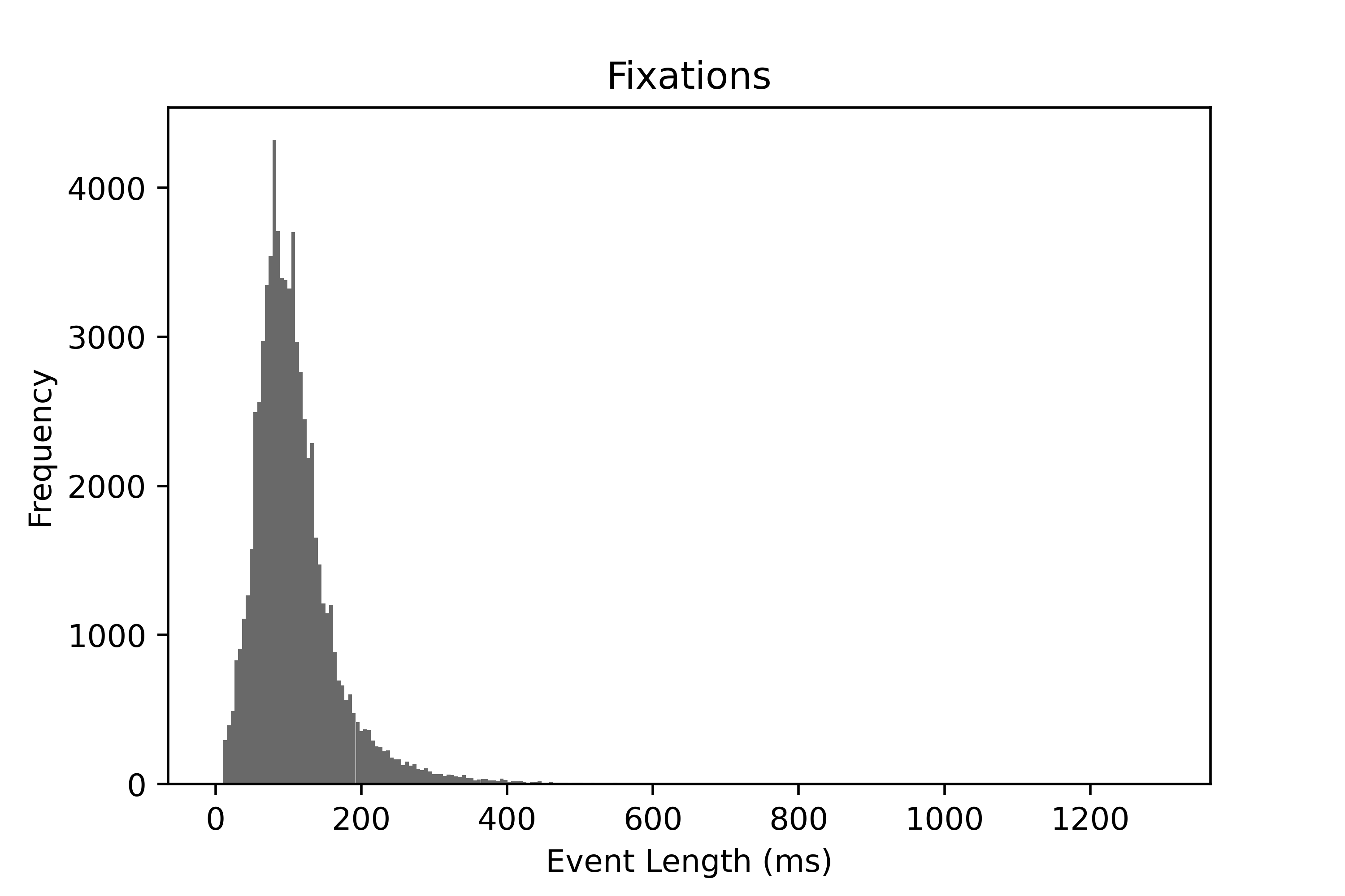
(a) Distribution of the fixation length

(b) Distribution of the saccade length

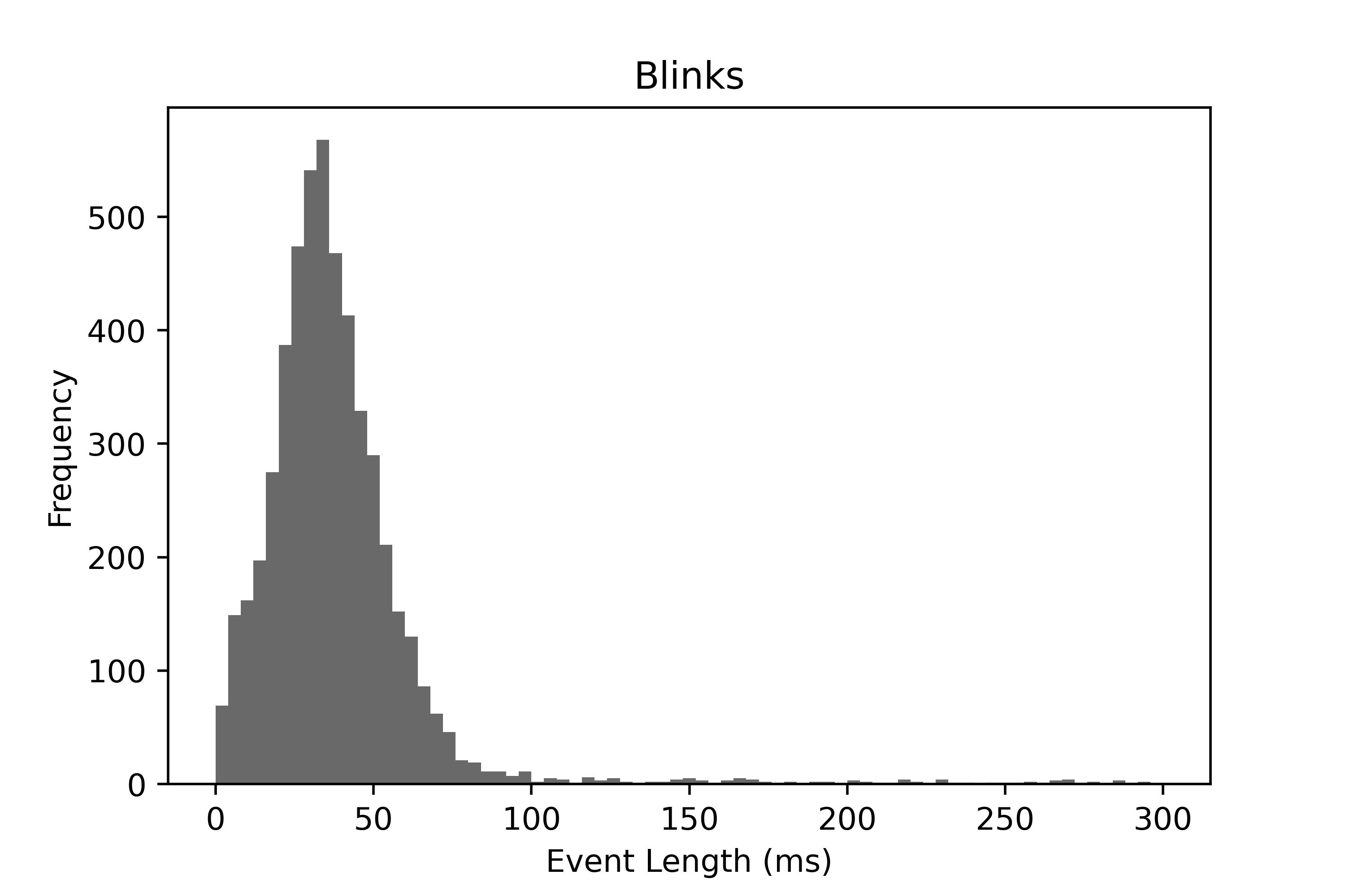
(c) Distribution of the blink length

Figure 7: Distribution of the length of each ocular event in the Natural Reading paradigm: fixations, saccades and blinks.

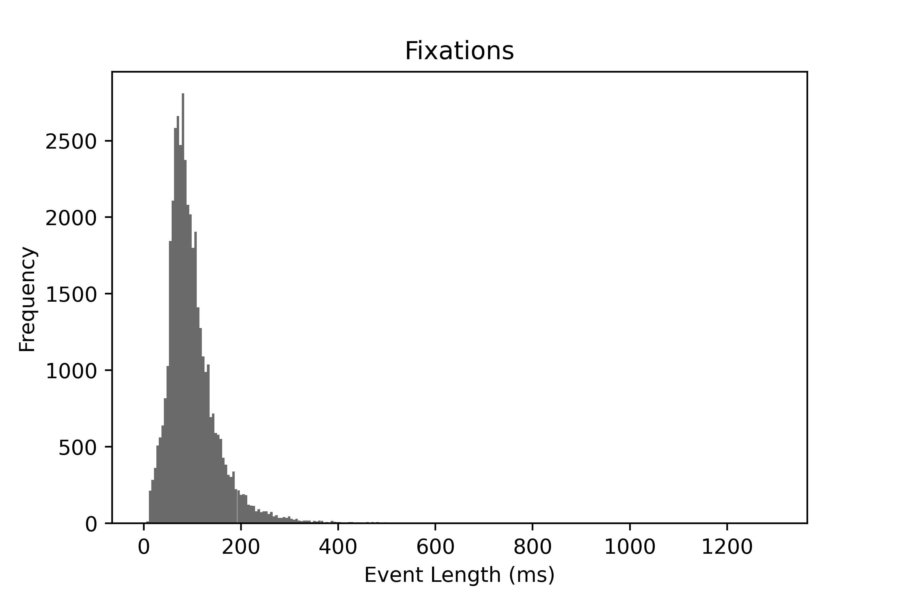
(a) Distribution of the fixation length

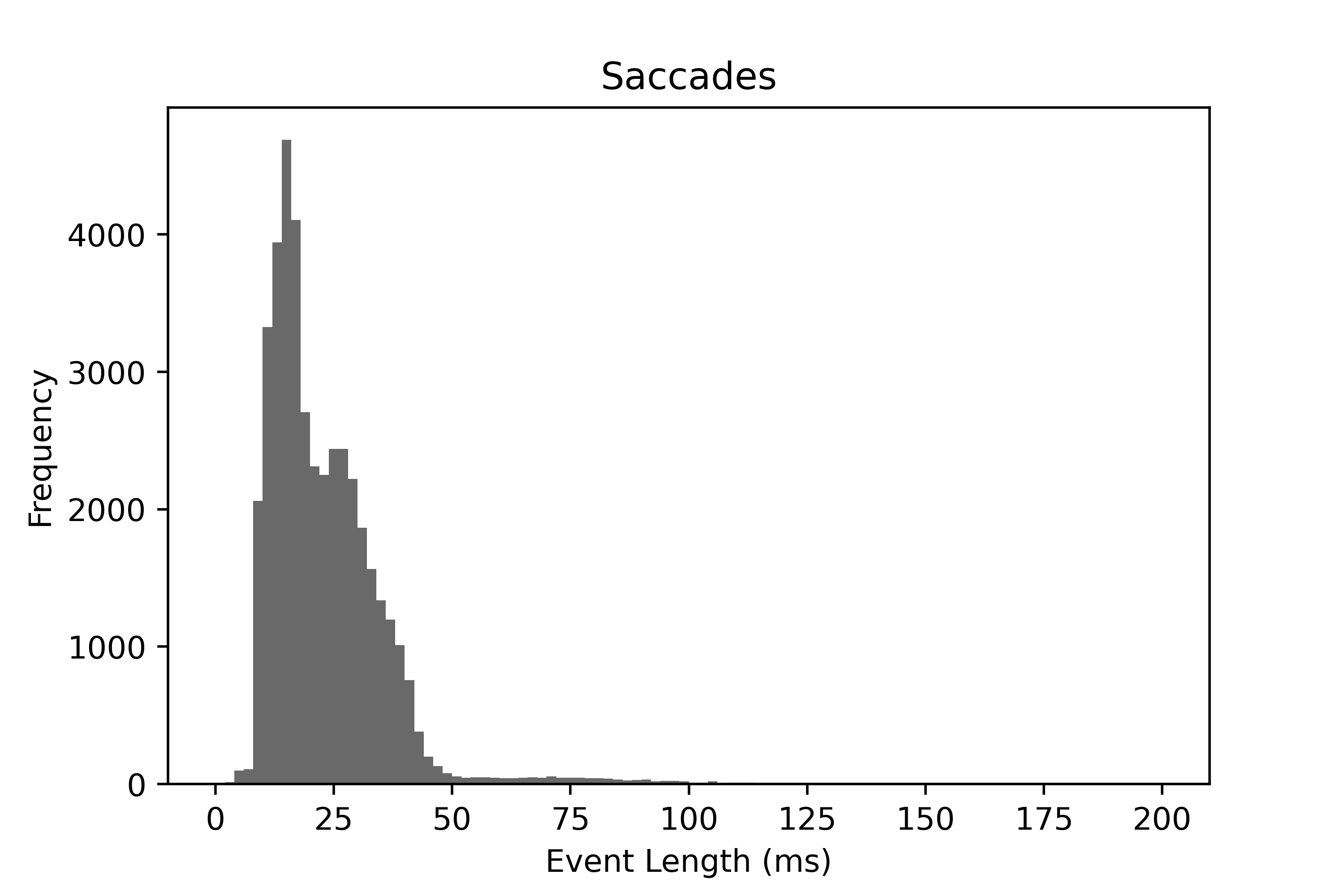
(b) Distribution of the saccade length

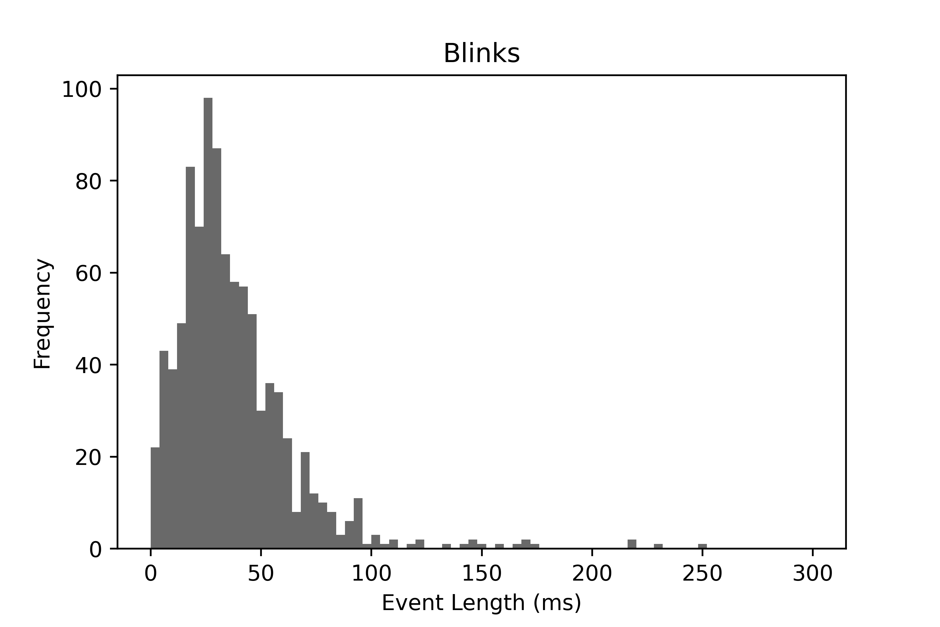
(c) Distribution of the blink length

Figure 8: Distribution of the length of each ocular event in the Visual Symbol Search paradigm: fixations, saccades and blinks.

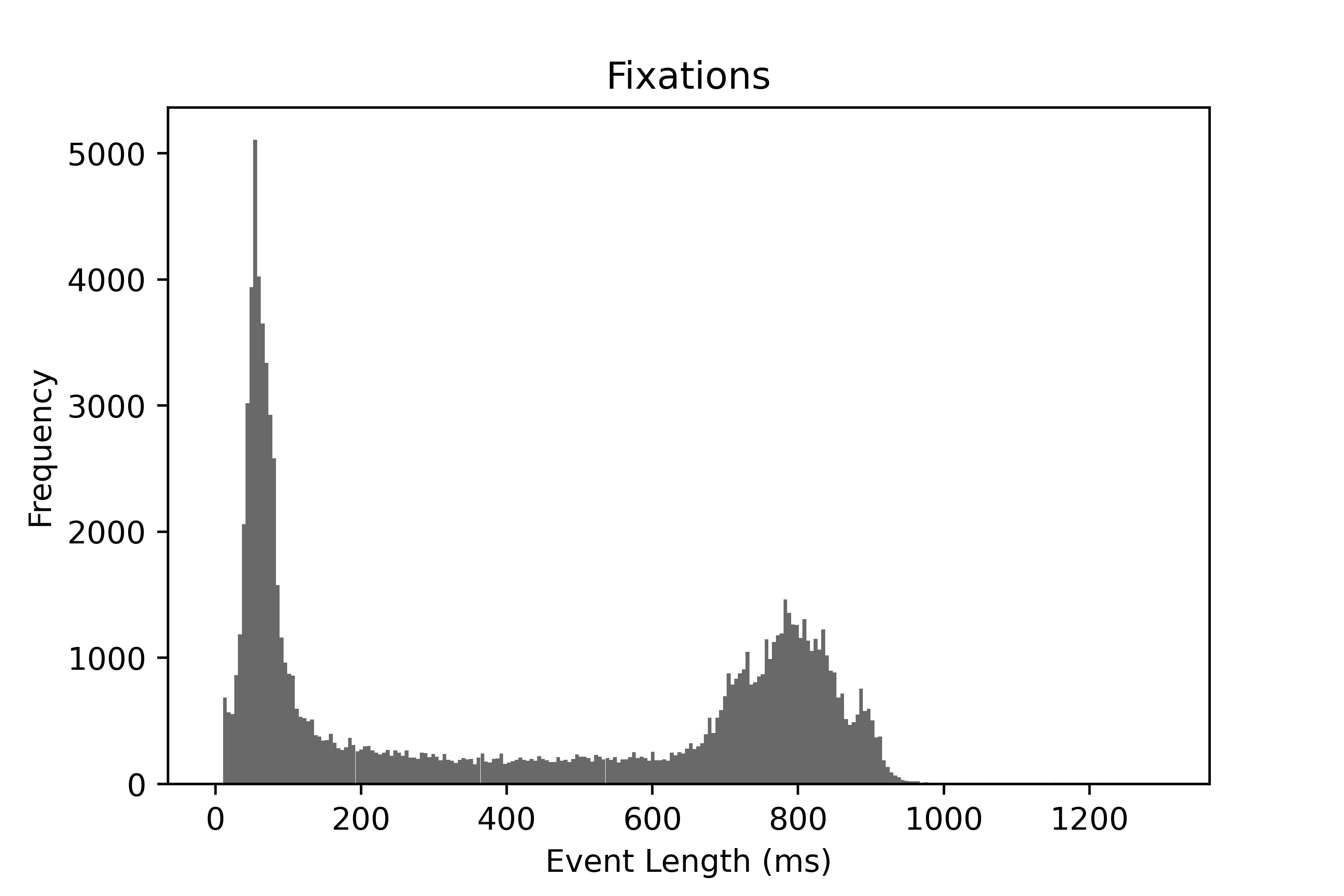
(a) Distribution of the fixation length

(b) Distribution of the saccade length

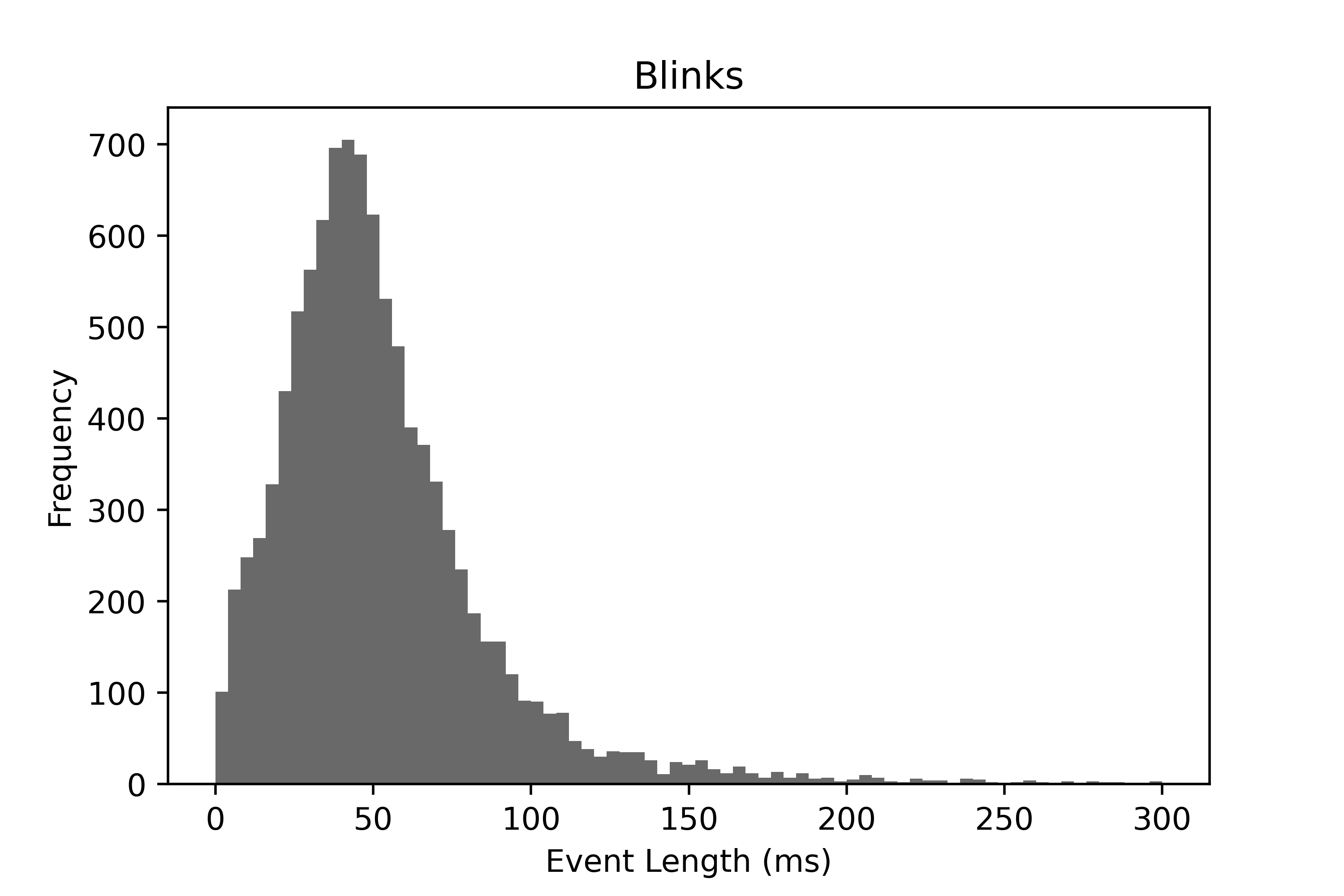
(c) Distribution of the blink length

Figure 9: Distribution of the length of each ocular event in the Large Grid paradigm: fixations, saccades and blinks.

References

- Barea et al. (2002) Barea, R., Boquete, L., Mazo, M., and López, E. System for assisted mobility using eye movements based on electrooculography. IEEE transactions on neural systems and rehabilitation engineering, 10(4):209–218, 2002.
- Behrens et al. (2010) Behrens, F., MacKeben, M., and Schröder-Preikschat, W. An improved algorithm for automatic detection of saccades in eye movement data and for calculating saccade parameters. Behavior research methods, 42(3):701–708, 2010.
- Buettner (2013) Buettner, R. Cognitive workload of humans using artificial intelligence systems: towards objective measurement applying eye-tracking technology. In Annual conference on artificial intelligence, pp. 37–48. Springer, 2013.
- Bulling & Roggen (2011) Bulling, A. and Roggen, D. Recognition of visual memory recall processes using eye movement analysis. In Proceedings of the 13th international conference on Ubiquitous computing, pp. 455–464, 2011.
- Bulling et al. (2009) Bulling, A., Ward, J. A., Gellersen, H., and Tröster, G. Eye movement analysis for activity recognition. In Proceedings of the 11th international conference on Ubiquitous computing, pp. 41–50, 2009.
- Carion et al. (2020a) Carion, N., Massa, F., Synnaeve, G., Usunier, N., Kirillov, A., and Zagoruyko, S. End-to-end object detection with transformers. In European Conference on Computer Vision, pp. 213–229. Springer, 2020a.
- Carion et al. (2020b) Carion, N., Massa, F., Synnaeve, G., Usunier, N., Kirillov, A., and Zagoruyko, S. End-to-end object detection with transformers. In European Conference on Computer Vision, pp. 213–229. Springer, 2020b.
- Chollet (2017) Chollet, F. Xception: Deep learning with depthwise separable convolutions. In Proceedings of the IEEE conference on computer vision and pattern recognition, pp. 1251–1258, 2017.
- de Cheveigné (2020) de Cheveigné, A. Zapline: A simple and effective method to remove power line artifacts. Neuroimage, 207:116356, 2020.
- Dimigen et al. (2011) Dimigen, O., Sommer, W., Hohlfeld, A., Jacobs, A. M., and Kliegl, R. Coregistration of eye movements and eeg in natural reading: analyses and review. Journal of experimental psychology: General, 140(4):552, 2011.
- Donahue et al. (2014) Donahue, J., Hendricks, L. A., Rohrbach, M., Venugopalan, S., Guadarrama, S., Saenko, K., and Darrell, T. Long-term recurrent convolutional networks for visual recognition and description, 2014. URL https://arxiv.org/abs/1411.4389.
- Engbert & Kliegl (2003) Engbert, R. and Kliegl, R. Microsaccades uncover the orientation of covert attention. Vision research, 43(9):1035–1045, 2003.
- Fawaz et al. (2020) Fawaz, H. I., Lucas, B., Forestier, G., Pelletier, C., Schmidt, D. F., Weber, J., Webb, G. I., Idoumghar, L., Muller, P.-A., and Petitjean, F. Inceptiontime: Finding alexnet for time series classification. Data Mining and Knowledge Discovery, 34(6):1936–1962, 2020.
- Fuhl et al. (2016) Fuhl, W., Tonsen, M., Bulling, A., and Kasneci, E. Pupil detection for head-mounted eye tracking in the wild: an evaluation of the state of the art. Machine Vision and Applications, 27(8):1275–1288, 2016.
- Goldberger AL (2000) Goldberger AL, Amaral LAN, G. L. H. J. I. P. M. R. M. J. M. G. P. C.-K. S. H. Physiobank, physiotoolkit, and physionet: Components of a new research resource for complex physiologic signals. Circulation 101(23):e215-e220, 2000.
- Hanke et al. (2019) Hanke, M., Mathôt, S., Ort, E., Peitek, N., Stadler, J., and Wagner, A. A practical guide to functional magnetic resonance imaging with simultaneous eye tracking for cognitive neuroimaging research. In Spatial Learning and Attention Guidance, pp. 291–305. Springer, 2019.
- Hollenstein et al. (2019) Hollenstein, N., Troendle, M., Zhang, C., and Langer, N. Zuco 2.0: A dataset of physiological recordings during natural reading and annotation. CoRR, abs/1912.00903, 2019. URL http://arxiv.org/abs/1912.00903.
- Holmqvist et al. (2011) Holmqvist, K., Nyström, M., Andersson, R., Dewhurst, R., Jarodzka, H., and Van de Weijer, J. Eye tracking: A comprehensive guide to methods and measures. OUP Oxford, 2011.
- Jacob & Karn (2003) Jacob, R. J. and Karn, K. S. Eye tracking in human-computer interaction and usability research: Ready to deliver the promises. In The mind’s eye, pp. 573–605. Elsevier, 2003.
- Jia et al. (2021) Jia, Z., Lin, Y., Wang, J., Wang, X., Xie, P., and Zhang, Y. Salientsleepnet: Multimodal salient wave detection network for sleep staging. CoRR, abs/2105.13864, 2021. URL https://arxiv.org/abs/2105.13864.
- Kappenman & Luck (2010) Kappenman, E. S. and Luck, S. J. The effects of electrode impedance on data quality and statistical significance in erp recordings. Psychophysiology, 47(5):888–904, 2010.
- Kastrati et al. (2021a) Kastrati, A., Plomecka, M. B., Pascual, D., Wolf, L., Gillioz, V., Wattenhofer, R., and Langer, N. Eegeyenet: a simultaneous electroencephalography and eye-tracking dataset and benchmark for eye movement prediction. CoRR, abs/2111.05100, 2021a. URL https://arxiv.org/abs/2111.05100.
- Kastrati et al. (2021b) Kastrati, A., Plomecka, M. B., Pascual, D., Wolf, L., Gillioz, V., Wattenhofer, R., and Langer, N. Eegeyenet: a simultaneous electroencephalography and eye-tracking dataset and benchmark for eye movement prediction. 2021b.
- Kastrati et al. (2021c) Kastrati, A., Plomecka, M. B., Wattenhofer, R., and Langer, N. Using deep learning to classify saccade direction from brain activity. In ACM Symposium on Eye Tracking Research and Applications, ETRA ’21 Short Papers. Association for Computing Machinery, 2021c.
- Keil et al. (2014) Keil, A., Debener, S., Gratton, G., Junghöfer, M., Kappenman, E. S., Luck, S. J., Luu, P., Miller, G. A., and Yee, C. M. Committee report: publication guidelines and recommendations for studies using electroencephalography and magnetoencephalography. Psychophysiology, 51(1):1–21, 2014.
- Kirillov et al. (2018) Kirillov, A., He, K., Girshick, R. B., Rother, C., and Dollár, P. Panoptic segmentation. CoRR, abs/1801.00868, 2018. URL http://arxiv.org/abs/1801.00868.
- Kleifges et al. (2017) Kleifges, K., Bigdely-Shamlo, N., Kerick, S. E., and Robbins, K. A. Blinker: Automated extraction of ocular indices from eeg enabling large-scale analysis. Frontiers in neuroscience, 11:12, 2017.
- Lawhern et al. (2018) Lawhern, V. J., Solon, A. J., Waytowich, N. R., Gordon, S. M., Hung, C. P., and Lance, B. J. Eegnet: a compact convolutional neural network for eeg-based brain–computer interfaces. Journal of neural engineering, 15(5):056013, 2018.
- Li et al. (2020) Li, X., Sun, X., Meng, Y., Liang, J., Wu, F., and Li, J. Dice loss for data-imbalanced nlp tasks, 2020.
- Lin et al. (2017) Lin, T.-Y., Goyal, P., Girshick, R., He, K., and Dollár, P. Focal loss for dense object detection. In 2017 IEEE International Conference on Computer Vision (ICCV), pp. 2999–3007, 2017. doi: 10.1109/ICCV.2017.324.
- Luna et al. (2008) Luna, B., Velanova, K., and Geier, C. F. Development of eye-movement control. Brain and cognition, 68(3):293–308, 2008.
- Mele & Federici (2012) Mele, M. L. and Federici, S. Gaze and eye-tracking solutions for psychological research. Cognitive processing, 13(1):261–265, 2012.
- Nyström & Holmqvist (2010) Nyström, M. and Holmqvist, K. An adaptive algorithm for fixation, saccade, and glissade detection in eyetracking data. Behavior research methods, 42(1):188–204, 2010.
- Paszke et al. (2019) Paszke, A., Gross, S., Massa, F., Lerer, A., Bradbury, J., Chanan, G., Killeen, T., Lin, Z., Gimelshein, N., Antiga, L., Desmaison, A., Kopf, A., Yang, E., DeVito, Z., Raison, M., Tejani, A., Chilamkurthy, S., Steiner, B., Fang, L., Bai, J., and Chintala, S. Pytorch: An imperative style, high-performance deep learning library. In Wallach, H., Larochelle, H., Beygelzimer, A., d'Alché-Buc, F., Fox, E., and Garnett, R. (eds.), Advances in Neural Information Processing Systems 32, pp. 8024–8035. Curran Associates, Inc., 2019.
- Pedregosa et al. (2011) Pedregosa, F., Varoquaux, G., Gramfort, A., Michel, V., Thirion, B., Grisel, O., Blondel, M., Prettenhofer, P., Weiss, R., Dubourg, V., Vanderplas, J., Passos, A., Cournapeau, D., Brucher, M., Perrot, M., and Duchesnay, E. Scikit-learn: Machine learning in Python. Journal of Machine Learning Research, 12:2825–2830, 2011.
- Pedroni et al. (2019) Pedroni, A., Bahreini, A., and Langer, N. Automagic: Standardized preprocessing of big eeg data. NeuroImage, 200:460–473, 2019.
- Perslev et al. (2019) Perslev, M., Jensen, M. H., Darkner, S., Jennum, P. J., and Igel, C. U-time: A fully convolutional network for time series segmentation applied to sleep staging, 2019.
- Perslev et al. (2021) Perslev, M., Darkner, S., Kempfner, L., Nikolic, M., Jennum, P. J., and Igel, C. U-sleep: resilient high-frequency sleep staging. npj Digital Medicine, 4(1):72, Apr 2021. ISSN 2398-6352. doi: 10.1038/s41746-021-00440-5. URL https://doi.org/10.1038/s41746-021-00440-5.
- Pettersson et al. (2013) Pettersson, K., Jagadeesan, S., Lukander, K., Henelius, A., Hæggström, E., and Müller, K. Algorithm for automatic analysis of electro-oculographic data. Biomedical engineering online, 12(1):1–18, 2013.
- Ronneberger et al. (2015) Ronneberger, O., Fischer, P., and Brox, T. U-net: Convolutional networks for biomedical image segmentation. CoRR, abs/1505.04597, 2015. URL http://arxiv.org/abs/1505.04597.
- Schmidt et al. (2018) Schmidt, J., Laarousi, R., Stolzmann, W., and Karrer-Gauß, K. Eye blink detection for different driver states in conditionally automated driving and manual driving using eog and a driver camera. Behavior research methods, 50(3):1088–1101, 2018.
- Sherstinsky (2018) Sherstinsky, A. Fundamentals of recurrent neural network (RNN) and long short-term memory (LSTM) network. CoRR, abs/1808.03314, 2018. URL http://arxiv.org/abs/1808.03314.
- Szegedy et al. (2017) Szegedy, C., Ioffe, S., Vanhoucke, V., and Alemi, A. Inception-v4, inception-resnet and the impact of residual connections on learning. In Proceedings of the AAAI Conference on Artificial Intelligence, number 1, 2017.
- Thoma (2016) Thoma, M. A survey of semantic segmentation. CoRR, abs/1602.06541, 2016. URL http://arxiv.org/abs/1602.06541.
- Toivanen et al. (2015) Toivanen, M., Pettersson, K., and Lukander, K. A probabilistic real-time algorithm for detecting blinks, saccades, and fixations from eog data. Journal of Eye Movement Research, 8(2), 2015.
- Vaswani et al. (2017) Vaswani, A., Shazeer, N., Parmar, N., Uszkoreit, J., Jones, L., Gomez, A. N., Kaiser, L., and Polosukhin, I. Attention is all you need. CoRR, abs/1706.03762, 2017. URL http://arxiv.org/abs/1706.03762.
- Wechsler (1955) Wechsler, D. Wechsler adult intelligence scale–. Archives of Clinical Neuropsychology, 1955.
- Wechsler & Kodama (1949) Wechsler, D. and Kodama, H. Wechsler intelligence scale for children, volume 1. Psychological corporation New York, 1949.
- Xu et al. (2020) Xu, G., Ren, T., Chen, Y., and Che, W. A one-dimensional cnn-lstm model for epileptic seizure recognition using eeg signal analysis. Frontiers in Neuroscience, 14:1253, 2020.
- Zemblys et al. (2018) Zemblys, R., Niehorster, D. C., and Holmqvist, K. gazenet: End-to-end eye-movement event detection with deep neural networks. Behavior research methods, 2018.